the impact of inventory leanness and slack resources on
TRANSCRIPT

Georgia State University Georgia State University
ScholarWorks @ Georgia State University ScholarWorks @ Georgia State University
Business Administration Dissertations Programs in Business Administration
Fall 12-11-2014
The Impact of Inventory Leanness and Slack Resources on Supply The Impact of Inventory Leanness and Slack Resources on Supply
Chain Resilience: An Empirical Study Chain Resilience: An Empirical Study
David J. Lyons Georgia State University
Follow this and additional works at: https://scholarworks.gsu.edu/bus_admin_diss
Recommended Citation Recommended Citation Lyons, David J., "The Impact of Inventory Leanness and Slack Resources on Supply Chain Resilience: An Empirical Study." Dissertation, Georgia State University, 2014. https://scholarworks.gsu.edu/bus_admin_diss/46
This Dissertation is brought to you for free and open access by the Programs in Business Administration at ScholarWorks @ Georgia State University. It has been accepted for inclusion in Business Administration Dissertations by an authorized administrator of ScholarWorks @ Georgia State University. For more information, please contact [email protected].

PERMISSION TO BORROW
In presenting this dissertation as a partial fulfillment of the requirements for an advanced degree
from Georgia State University, I agree that the Library of the University shall make it available
for inspection and circulation in accordance with its regulations governing materials of this type.
I agree that permission to quote from, to copy from, or publish this dissertation may be granted
by the author or, in his/her absence, the professor under whose direction it was written or, in his
absence, by the Dean of the Robinson College of Business. Such quoting, copying, or publishing
must be solely for the scholarly purposes and does not involve potential financial gain. It is
understood that any copying from or publication of this dissertation which involves potential
gain will not be allowed without written permission of the author.
David J. Lyons

NOTICE TO BORROWERS
All dissertations deposited in the Georgia State University Library must be used only in
accordance with the stipulations prescribed by the author in the preceding statement.
The author of this dissertation is:
David J. Lyons
J. Mack Robinson College of Business
Georgia State University
35 Broad Street, NW
Atlanta, Georgia 30303
The director of this dissertation is:
Dr. Patricia G. Ketsche
Department of Health Administration
J. Mack Robinson College of Business
Georgia State University
35 Broad Street, Suite 806
Atlanta, GA 30303

The Impact of Inventory Leanness and Slack Resources on Supply Chain Resilience: An
Empirical Study
BY
David Jerome Lyons
A Dissertation Submitted in Partial Fulfillment of the Requirements for the Degree
Of
Executive Doctorate in Business
In the Robinson college of Business
Of
Georgia State University
GEORGIA STATE UNIVERSITY
ROBINSON COLLEGE OF BUSINESS
2014

Copyright by
David Jerome Lyons
2014

ACCEPTANCE
This dissertation was prepared under the direction of the David J. Lyons Dissertation Committee.
It has been approved and accepted by all members of that committee, and it has been accepted in
partial fulfillment of the requirements for the degree of Doctoral of Philosophy in Business
Administration in the J. Mack Robinson College of Business of Georgia State University.
Richard D. Phillips, Dean
DISSERTATION COMMITTEE
Dr. Patricia G. Ketsche (Chair)
Dr. Adrian Souw-Chin Choo
Dr. Michael J. Gallivan

v
TABLE OF CONTENTS
CHAPTER 1: INTRODUCTION ....................................................................................... 1
1.1 Research Domain ............................................................................................. 1
1.2 Background...................................................................................................... 6
1.2.1 Motivation for the study ......................................................................... 6
1.2.2 Significance of the study .................................................................... 7
1.2.3 Theoretical and conceptual framework ............................................... 8
1.3 Research Questions .......................................................................................... 9
CHAPTER 2: LITERATURE REVIEW ............................................................................ 11
2.1 Supply Chain Resilience ................................................................................. 11
2.1.1 Disruptions ......................................................................................... 12
2.2 Supply Chain Performance .............................................................................. 12
2.2.1 Leanness ............................................................................................ 13
2.2.2 Slack resources ................................................................................... 14
CHAPTER 3: CONCEPTUAL MODEL AND HYPOTHESES ......................................... 17
3.1 Conceptual Model ........................................................................................... 17
3.2 Hypotheses Development ................................................................................ 19
3.2.1 Variables ............................................................................................ 20
3.2.2 Control Variables ............................................................................... 23
3.3 Summary ........................................................................................................ 30
CHAPTER 4: RESEARCH METHODOLOGY AND DATA COLLECTION ................... 32
4.1 Research Design ............................................................................................. 32
4.2 Research Philosophy ....................................................................................... 32
4.3 Research Method ............................................................................................ 33
4.4 Data Collection ............................................................................................... 33
4.5 Data Preparation ............................................................................................. 34
CHAPTER 5: QUANTITATIVE ANALYSIS AND RESULTS ........................................ 35
5.1 Results ........................................................................................................... 35
5.1.1 Hypotheses 1a – 1d............................................................................. 35
5.1.2 Hypotheses 2a and 3a ......................................................................... 45
5.1.3 Hypotheses 2b and 3b ......................................................................... 46
5.1.4 Hypothesis 4 ....................................................................................... 47
5.1.5 Hypothesis 5 ....................................................................................... 48
5.1.6 Determinants of firm performance in the post-recession period ..................... 49

vi
CHAPTER 6: DISCUSSION AND IMPLICATIONS ........................................................ 52
6.1 Summary of Results and Discussion ............................................................... 52
6.2 Theoretical Contributions................................................................................ 59
6.3 Contributions to Practice ................................................................................. 60
6.4 Limitations of the Study .................................................................................. 62
6.5 Future Research .............................................................................................. 65
BIBLIOGRAPHY ........................................................................................................... 67
vii
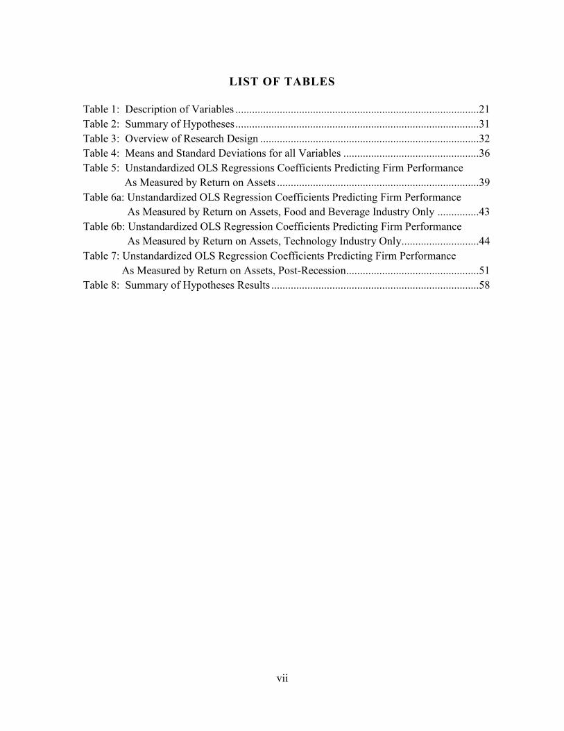
LIST OF TABLES
Table 1: Description of Variables ........................................................................................21
Table 2: Summary of Hypotheses ........................................................................................31
Table 3: Overview of Research Design ...............................................................................32
Table 4: Means and Standard Deviations for all Variables .................................................36
Table 5: Unstandardized OLS Regressions Coefficients Predicting Firm Performance
As Measured by Return on Assets .........................................................................39
Table 6a: Unstandardized OLS Regression Coefficients Predicting Firm Performance
As Measured by Return on Assets, Food and Beverage Industry Only ...............43
Table 6b: Unstandardized OLS Regression Coefficients Predicting Firm Performance
As Measured by Return on Assets, Technology Industry Only ............................44
Table 7: Unstandardized OLS Regression Coefficients Predicting Firm Performance
As Measured by Return on Assets, Post-Recession................................................51
Table 8: Summary of Hypotheses Results ...........................................................................58

viii
LIST OF FIGURES
Figure 1: Conceptual Model ................................................................................................18
Figure 2: Combined Variables .............................................................................................25

ix
ABBREVIATIONS
List of Abbreviations [in Alphabetical Order]
DOI ................Days of Inventory
DV ..................Dependent Variable
F&B................Food and Beverage
OLS ................Ordinary Least Squares
Q ....................Quarter (a fiscal period of 3 months)
ROA ..............Return on Assets
SC ...................Supply Chain
VIF .................Variance Inflation Factor
WCR ..............Working Capital Ratio

x
ABSTRACT
The Impact of Inventory Leanness and Slack Resources on Supply Chain Resilience: An
Empirical Study
BY
David Jerome Lyons
Committee Chair: Dr. Patricia G. Ketsche
Major Academic Unit: Department of Health Administration
When a major disruption occurs, an organization’s performance is usually negatively
affected. The great recession of 2008 – 2009 was such a disruption which had global
implications that had not been seen since the great depression that started in the 1930s. This
thesis is intended to contribute to the understanding of how leanness and slack resources affect
firm performance in the presence of disruptions that test supply chain resilience, or the ability to
restore the firm’s performance to its original condition after encountering stress or a large
disturbance. These disruptions may not only affect the firm’s financial performance during the
disruption but also well after the disruption has occurred. Two industries with differing supply
chains, food and beverage, and electronics and computer, were investigated. The study is based
on archival data (N=10,020 and 668 firms) with observations from just before and just after the
great recession, a disruption that affected the entire global economy.
Our results suggest (1) the effect of inventory leanness and slack resources on firm
performance is industry specific; and (2) variation in firm performance is less in the post-
disruptive period than in the pre-disrupted period. Overall, our findings call for a contingency

xi
perspective to specify the level of inventory leanness and slack resources when determining their
impact on firm performance to support supply chain resilience.

1
1.0 INTRODUCTION
1.1 Research Domain
Toward the end of 2007, the global financial crisis rapidly moved from a housing bubble
in the United States to the worst recession the world has witnessed for over six decades. This
great recession created financial turbulence that was collectively not seen globally since The
Great Depression of the 1930’s. The crisis came as a surprise to many academics, managers,
policymakers, and investors (Verick & Islam, 2010). Galbraith (2009) provided an argument
that “the implicit and explicit intellectual collusion made it difficult for members of the
profession (primarily associated with American universities) to predict an alternative view, and
the severity of the global financial crisis was underestimated” (p. 87). This worldwide
economic crisis in 2008-2009 reduced the amount of money that was available to many firms.
Leveraged mistakes in working capital in supply chains became obvious and toxic; in fact, some
supply chain networks would have been on the verge of collapse if liquidity deficiencies among
suppliers had not been balanced by financially strong firms within the supply chain. This crisis
created a freezing of capital and an inability of organizations to expand and grow (Lux &
Westerhoff, 2009). Disruptions, especially supply chain disruptions, often are unpredictable,
occur quickly and have lasting effects. In the last few years, over 85 percent of firms worldwide
have experienced at least one major disruption ("Supply Chain Resilience," November, 2012).
These disruptions can come in many different forms; for example, an oil spill in the Gulf of
Mexico, political and social unrest in Africa and Middle East, and/or an earthquake and
subsequent tsunami in Japan. The great recession, which is an example of one such disruption,
triggered a global financial panic that was followed by reduced asset values and freezing of
credit flows.

2
The great recession began with a collapse in housing prices in the United States, which
triggered a financial panic because of the opaque nature of securitized mortgage instruments,
which quickly became "toxic assets." The financial panic was followed by the collapse of real
activity as the result of reduced asset values and the freezing up of credit flows. As the crisis
deepened in the advanced economies, projections for the world economy became more uncertain
(Verick, 2010). The increase in worldwide economic and political uncertainty acted like a
"tsunami effect" that sharply reduced productive asset values throughout the world. Stock
markets around the globe responded accordingly with significant corrections.
A lesson from the great recession is that firms need to prepare for not only unanticipated
financial disruptions, but also for any significant disruption. As a firm moves from a period of
normal activity through a disruption and then back to a more normal state, financial performance
is often negatively affected during and for a long period after the disruption. Resiliency within a
firm supports the recovery from a disruption (Lengnick-Hall, Beck, & Lengnick-Hall, 2011).
Building resiliency is an investment in a firm’s future (Reinmoeller & Van Baardwijk, 2005).
Like any other type of investment, investment in resiliency is often difficult and costly. A key
lesson from the recent past, however, is that while investments in resiliency can be too extreme
and costly, they should not be undervalued (Grusky, Western, & Wimer, 2011; Montiel, 2011).
The need for resiliency in a firm’s supply chain (SC) has been studied extensively by
researchers (Beamon, 1999; Chen & Miller-Hooks, 2012; Christopher & Holweg, 2011; Horne,
1997; Kleindorfer & Saad, 2005; Pettit, Fiksel, & Croxton, 2010). However, the research
performed on this topic is by no means complete, and process models studying the effect of lean
and slack resources on a firm’s resiliency prior to and after a significant disruption is of great
interest for researchers and practitioners. Many researchers have formulated assessment tools to

3
identify and implement SC resiliency, identify the components of SC resiliency, define SC
resiliency, and articulate how to design and simulate SC’s for resiliency (Blackhurst, Dunn, &
Craighead, 2011; Christopher & Peck, 2004; Ellis, Shockley, & Henry, 2011; Hendricks &
Singhal, 2005b; Pettit et al., 2010). Yet despite this significant amount of research on SC
resiliency, there is a paucity of research on the pre- versus post-disruption interaction of
resilience in the face of a significant disruption, especially with respect to global implications.
Also, the effect of leanness and slack has not been included in this interaction by prior
researchers.
Leanness, and specifically inventory leanness, is included in this study to aid in
understanding the role that a widely adopted inventory management practice plays in reducing
costs. When firms are faced with an economic environment that disrupts their ability to meet
expected profit levels and the expectations of their stakeholders, they often resort to emphasizing
lean practices to aid in the recovery efforts (Lewis, 2000; Pettersen, 2009). Lean practices in a
firm are expected to result in improved operational outcomes, such as a reduction in required
levels of inventory, which therefore should enhance firm performance (Eroglu & Hofer, 2011).
Lean practices, or more specifically lean production, is often described as a philosophy or a
strategy with a set of practices (e.g. total quality management, value stream mapping, etc.) which
seeks to minimize or eliminate waste (e.g. excess inventory, rework, delays, etc.) to improve firm
performance (Eroglu & Hofer, 2011). Leanness in a supply chain supports maximizing profit
through cost reduction (Agarwal, Shankar, & Tiwari, 2006). There is thus a linkage between the
larger concept of lean production principles and inventory leanness (Eroglu & Hofer, 2011).
Conversely, slack resources provide a cushion or pool of resources that are available to
an organization to adapt to internal or external pressures, as well as initiate adjustments with

4
respect to the external environment (Bourgeois, 1981). These excess resources can be viewed as
a buffer that is waste or the results of improper management of inventory. In a neoclassical
view, slack would only be present when a firm is not in an equilibrium state and should be
minimized for the sake of efficiency (Sharfman, Wolf, Chase, & Tansik, 1988). Thompson,
Scott, and Zald (2009) argue that slack should be used to provide protection to the firm from its
external environment. Slack is included in this study due to the constant tension that SC
managers face to have proper balance between operational efficiency and lean practices, while
simultaneously meeting the demand to have surplus resources available to prepare for
unexpected threats or disruptions.
Firm size may affect a firm’s capability to achieve increased competitiveness and
financial performance. Garmestani, Allen, Mittelstaedt, Stow, and Ward (2006) found that
periods of uncertainty have significantly greater effect on survivability of small firms than large
firms. Larger business units tend to have a larger market size and greater control over the
competitive environment, combined with access to resources that are not as available to a smaller
firm1 (Beck et al., 2005). Firms with fewer resources, such as small firms, may be unable to
afford strategies that include slack resources (Raisch & Birkinshaw, 2008). Additionally, small
firms may not have the power and influence to change the behavior of other supply chain
partners to help recover from the disruption as do large firms (Kuper, 2002). Therefore, I focus
exclusively on the category of large firms and control for firm size in this study.
Industries often have differing inventory patterns and product life cycles. These patterns
and life cycles are often due to fast changing consumer preferences, as well as the rate of
1 Large firms are often determined as those that employ more than 500 employees. Annual revenue is also a
measure to differentiate between smaller and larger firms (Beck, Demirgüç-Kunt, & Maksimovic, 2005). The
threshold is established at annual revenue for larger firms greater than one hundred million dollars. Revenue is a
compatible measure for categorizing firm size when studying quantitative measures, i.e., inventory, cash, and other
financial resources (Lev, 1969).

5
innovation. Different inventory levels are often due to seasonality, production capability, raw
material availability, storage capability, or product shelf life. The consumer electronics and
computer industries (i.e., technology industries) are prime examples of a short life cycle industry
with high inventory turns. In contrast, the food and beverage industries life cycles and inventory
turns are considered longer due to less innovation, capital intensity for manufacturing and
distribution, and slower fad effects (Kurawarwala & Matsuo, 1996), as is the case with soft
drinks or packaged foods. The food and beverage industries also have inventory dynamics that
often increase inventories due to raw materials that have a short shelf life and can be limited to
seasonal harvests. Including both the food and beverage and the electronics and computer
industries in this study provides a dichotomy of inventory management patterns that encompass
the wide diversity of inventory volumes and velocities due to demand characteristics,
complexity, volume of stock keeping units, and channels of distribution. This diversity between
the two industries will support generalizing the findings across the consumer goods segment of
which these industries are included.
An organization's pre disruption and post disruption performance is often determined in
part by the organization's resources and capabilities at the start of the disruption. Firm size,
profitability, and diversification can have an effect on short- and long- term performance.
“Short-termism” specifically emerges when managers are driven to invest current resources
during disrupted economic periods, thereby putting pressure on cost reduction initiatives. In
short, these responses to recessionary pressure indicate management's short-term objective to get
"lean and mean" (Latham & Braun, 2011). The short term economic period is often within a
fiscal year, and any business period beyond that time is considered long-term (Fama & French,
1989). Going beyond the short-term period, this study will include data that spans for more than

6
one fiscal year. In other words, this study will include time periods in the pre and post disruption
periods so as to provide a longer-term view. The pre-recessionary time period in this study will
include the first quarter of 2007 to the fourth quarter of 2008, as well as the post-recessionary
time periods of the first quarter of 2010 to the fourth quarter of 2011. Theses pre and post
disruption time periods will support the long-term view beyond short-term effects (Rothaermel &
Hill, 2005).
1.2 Background
1.2.1 Motivation for the study. As stated earlier, most firms have experienced a major
disruption in the recent past. It was a disruption that, in some way, significantly affected almost
every firm, whether they were global or not, or large or small (Grusky et al., 2011). Firms are
affected by a disruption in different ways, determined in part by the type of disruption (Rao &
Goldsby, 2009). Economic recessions are often the most transformative event that an
organization will face. Additionally, not all firms within an industry will have the capabilities to
survive or adapt to the new economic reality post hoc a recession. While the disruptive nature of
an economic recession is widely acknowledged by practitioners and academics alike, scant
research has addressed how supply chain managers can successfully maneuver through these
turbulent events (Latham & Braun, 2011).
1.2.2 Significance of the study. A majority of the supply chain management efforts in
the recent past have focused on increasing the efficiency (lowering costs, lean practices) of the
supply chain operations, and less on managing the risks of potential disruptions. The carrying
cost of inventory in the consumer goods industries often ranges between 8 percent to 15 percent
of sales (Dullaghan, Harcourt, McCarthy, & Raftery, 2001). This high level of cost becomes a
prime target by managers seeking savings. Much of the recent academic literature on supply

7
chain models also seems to be focused on managing costs. This focus could be partly because
improving efficiency is an ongoing activity at most firms. Managers have developed the
necessary skills to focus on cost reduction, and they know how to justify and manage resources
that improve efficiency (Cecere & Chase Jr., 2013). Rationale for retaining slack resources is
limited, especially when carrying costs for such resources are high. Major supply chain
disruptions are infrequent and they are hard to predict and manage. Thus, it is difficult to justify
consistently and proactively devoting resources to managing such risks (Hendricks & Singhal,
2005b).
Lean production philosophy sees inventory as a form of waste to be minimized (Jones,
Roos, & Womack, 1990). Leanness in inventory is often viewed by supply chain management as
a means to improve financial performance, especially when the stress of a disruption is placed on
an organization (Levy, 1997). While lower inventories may improve a firm’s cash position or
working capital (thereby creating financial slack resources), emphasis upon lowering inventory
stock may jeopardize the ability to support a supply-side disruption (Zsidisin & Wagner, 2010).
Nonetheless, lean practices are widely implemented, and under normal circumstances their
implementation results in improved financial performance (Fullerton & McWatters, 2001).
However, it is not clear whether such a focus enhances a firm’s resiliency.
One definition of resiliency is the ability to cope with externalities and restore normal
operations to its original state, or move to a new and more desirable state after being disrupted
(Chen & Miller-Hooks, 2012; Christopher & Peck, 2004; Sheffi, 2005). Based on the
foundations of life and social sciences, this perspective of resilience has been adapted to supply
chain management (Martin-Breen & Anderies, 2011). It is important that supply chain managers
understand the role of inventory leanness and slack resources in enhancing or reducing a firm’s

8
resiliency when faced with a significant disruption. From a theoretical perspective, supply chain
and lean philosophy researchers would benefit from having a greater understanding of the
determinants of resilience and the approach of firms managing inventory leanness and slack
resources during episodes of turbulence.
1.2.3 Theoretical and conceptual framework. This thesis empirically examines the
effects of inventory leanness and slack resources on firm performance prior to and after a major
global disruption that tests the presence of supply chain resiliency in a firm.
Supply chain resilience has varying viewpoints, and it draws from multiple disciplines,
including psychology and ecology (Martin-Breen & Anderies, 2011). Although there have been
many definitions proposed for supply chain resilience, there is an underlying assumption that
resilient organizations prosper in dynamic environments (Cho, Mathiassen, & Robey, 2006).
Among scholars, there are two approaches when evaluating or describing organizational
resilience. Some see resilience as the ability of an organization to rebound from unanticipated
adverse disruptions to their pre-disrupted performance level, while others see organizational
resilience as having the dynamic capability to rapidly recover, adapt, and emerge from the
disrupted conditions with new capabilities strengthened and more resourceful (Ponis, 2012).
Resilience is applied in this thesis as a theoretical construct that subscribes to the former
description, whereby if a firm returns to its prior level of financial performance after the
disruption, then the firm would be determined to have resiliency.
Much of the ongoing supply chain management efforts at most firms over the last several
decades have been focused on lowering costs. This is where managers have honed their skills to
deliver performance, and upper level leaders have focused on allocating resources, including
training and incentives, to drive performance through cost containment (Cecere & Chase Jr.,

9
2013). Placing greater emphasis on lean activities, Womack and Jones (2010) argue that an
organization should never relax until it reaches perfection, which is defined as the delivery of
pure value instantaneously with zero waste. In other words, the implementation of lean practices
should be relentlessly pursued because these practices will lead to improved operational
performance outcomes which will, in turn, continue to enhance firm performance. Lean
practices are an important multi-dimensional construct that have a positive influence as an
antecedent in firm performance (Fullerton & McWatters, 2001; Inman & Mehra, 1993).
Under normal conditions, the relentless pursuit of efficiency does in fact lead to improved
financial performance (Jones et al., 1990). However, as disruptions or threats to the supply side
occur, being lean in inventory can negatively affect a firm’s performance if the firm is unable to
competitively fulfill demand. There is some evidence that in the longer term, slack resources are
necessary for survival and effectiveness (profit optimization) of the firm (Sharfman et al., 1988).
Thus, the foundational basis for this study is that slack resources support firm performance as a
firm navigates the effects of a disruption, and firms will place an emphasis on inventory leanness
over slack resources due to the view that slack represents waste that should be eliminated while
lean practices are relentlessly pursued.
1.3 Research Questions
Because of the many disruptions, whether they are economic, environmental, or
geopolitical that have affected organizations, especially in the last two decades, there is abundant
research defining, assessing, modeling, and examining disruptions on supply chain resiliency and
firm performance (Kleindorfer & Saad, 2005). However, there is a paucity of research on
understanding the relationship between supply chain resiliency and firm performance through a
virtually ubiquitous disruption like the great recession. Once a firm experiences a disruption,

10
managers will often reflect to understand what changes in practice should occur to prepare for a
future perturbation (Ketchen, Rebarick, Hult, & Meyer, 2008). With the popularity and
widespread adoption of lean practices, the reduction of inventories is primary within those
practices (Eroglu & Hofer, 2011; Huson & Nanda, 1995).
Lean principles have been adopted at some level by most manufacturing firms (Womack
& Jones, 2010), while a lack of attention has been applied by most firms toward slack resources
(Daniel, Lohrke, Fornaciari, & Turner Jr, 2004). Often these principles of leanness and slack are
primarily applied to reduce cost and improve firm performance and often not in balance. A
nuanced understanding of these principles is likely to benefit SC managers and executives to
prepare for the next inevitable disruption. As a result, this study is intended to explore the
following questions:
1. Does a firm’s focus on inventory leanness and slack resources in the firm have an
effect on firm performance under conditions of an economic disruption?
2. Is a firm’s supply chain resiliency affected by its inventory leanness and slack
resources under conditions of an economic disruption?

11
2.0 LITERATURE REVIEW
2.1 Supply Chain Resilience
Resilience is the theoretical perspective used in the design and implementation of this
research study. Historically, resilience has been a key concept in the fields of ecology and
psychology, and lately it has a strong presence in planning and organizational management
(Martin-Breen & Anderies, 2011). In the realm of enterprises, the concept of organizational
resilience emerges as a relatively new area in organizational theory that includes insights from
both coping and contingency theories (Gittell, 2008). Resilience in an organization can be a
single level or multiple level construct. When considering the ecological concept it favors the
science of engineering. Within the engineering material science, resilience is often viewed as
restoring to its original condition or returning to normal after encountering stress, a large shock,
strain or disturbance (Christopher & Peck, 2004; Horne, 1997; Mandal, 2012; Martin-Breen &
Anderies, 2011). The other stream of organizational resilience visualizes it beyond restoration to
include the development of new capabilities, creating new opportunities and emerging from the
disruption strengthened and more resourceful (Jüttner, 2005; Pettit et al., 2010; Ponomarov &
Holcomb, 2009). Although a robust, agile, and capable supply chain may be desirable, it is
important to note that a robust, agile, and capable does not always equate to a resilient supply
chain (Christopher & Holweg, 2011). These adaptive capabilities may not support the means to
respond and recover at the same or better state of performance (Jüttner & Maklan, 2009).
A focus on supply chain is highly regarded as one of the most effective ways for firms to
enhance their competitive advantage and firm performance. There is a highly positive
relationship between supply chain performance and firm performance (Ou, Liu, Hung, & Yen,
2010). As firms experience a disruption, their performance often declines. Resilient firms are

12
able to quickly emerge from a disruption to their performance level just prior to the disruption or
to a greater level of performance (Christopher & Peck, 2004; Mandal, 2012).
2.1.1 Disruptions. Disruptions manifest themselves in many different forms, and as
supply chains increase the distance of their network, become more global, and shorten the time
required between transactions or cycle time through strategies such as lowering their inventory
levels, disruptions seem to be more severe (Blackhurst , Craighead, Elkins, & Handfield, 2005;
Zsidisin & Wagner, 2010). Additionally, SC disruptions can negatively impact productivity and
utilizations of assets. For example, firms may end up with excess inventory for some products
and out of stock for others, a fact that can negatively affect customer service if customers cannot
receive the products they want when they want them. These symptoms of a disruption can also
negatively affect a firm’s reputation and credibility in the mind of investors, customers, and
suppliers (Hendricks & Singhal, 2003).
Christopher & Peck (2004) state “in today’s uncertain and turbulent markets, supply
chain vulnerability has become an issue of significance for many companies”, and that “as
supply chains become more complex as a result of global sourcing and the continued trend to
‘leaning down’, supply chain risks increase” (p. 4067). Moreover, as companies increasingly
compete with other supply chains “the challenge to business is to manage and mitigate that risk
through creating more resilient supply chains” (Christopher & Peck, 2004, p. 4067).
2.2 Supply Chain Performance
Hendricks and Shinghal (2005b) show that firm operating performance is eroded and that
capital markets penalize organizations that experience supply chain disruptions. Wagner and
Bode (2008) suggest that supply-side risks have a negative impact on supply chain performance.
To minimize loss of firm performance from disruptions, attention must be given to the supply

13
chain and the overall efficiency of the supply chain under normal operations. Over the last two
decades, the importance of leanness has been emphasized in internal operations, as well as in the
extended enterprise (Hofer, Eroglu, & Rossiter Hofer, 2012). Much less attention has been given
to the tradeoff between leanness and supply chain robustness. Supply chain robustness in this
sense is defined as the time it takes to go from disruption to a return to 100% capacity (Womack
& Jones, 2010). Resilient supply chains are not detrimental or inimical to efficiency and lean
operations, but the dimensions of the supply chain must be explicitly considered in the design
process of the supply chain (Kleindorfer & Saad, 2005). Whereas resilient capabilities are not
excess or waste but complimentary and should be a part of the overall lean supply chain design.
Lean management practices are a key construct in supply chain management theory building
(Chen & Paulraj, 2004).
2.2.1 Leanness. Lean philosophy has become popular and has been evolving since the
1980’s (Jones et al., 1990). Toyota Motor Company was the company that many firms emulated
in the operational waste reduction efforts that defined leanness. Specifically, “waste is any
human activity which absorbs resources but creates no value” (Womack & Jones, 2010, p. 15).
Lean inventory has become synonymous with good inventory control (Cooper & Maskell, 2008).
Inventory leanness is an outcome of lean practices and has been shown to result in improved
operational performance, which in turn should enhance firm performance (Eroglu & Hofer,
2011; Fullerton, McWatters, & Fawson, 2003). However, there are other studies that have found
no significant effects of lean production practices on firm performance (Huson & Nanda, 1995;
Jayaram, Vickery, & Droge, 2008). One reason for this finding is that greater product variety
that can increase the burden rate on product cost that is greater than the savings from lean efforts.
In addition, the need for a systemic focus on lean strategy, design, and manufacturing stands in

14
contrast to the potential benefit of focusing on a few segments or subsystems, and integration of
business processes, not just functions. Inventory is generally created based upon anticipated
future demand and production capabilities (Jones et al., 1990). It is possible that certain
industries may be more responsive to lean inventory systems than others due to characteristics of
markets, technologies or other environmental factors (Eroglu & Hofer, 2011). Additionally, it is
possible that when inventory levels are high, focus on inventory leanness effectively enhances
firm performance, but at some point additional focus on leanness may have negative effects on
performance. The current research project will explore that potential relationship.
The application of inventory leanness in firms can provide valuable insight on how
organizations influence performance and withstand significant disruptions to their supply chain
and their overall business. Research has hinted that once a disruption (especially in the case of a
recession) concludes, some firms may continue with their lean strategies that may ultimately
compromise the organization (Hendricks & Singhal, 2005b). In other words, a firm’s continued
myopic focus on lean strategies and “belt tightening’ efforts after the disruption may stifle
exploratory efforts of innovation, market growth, and investment.
2.2.2 Slack resources. Slack resources are defined as “the difference between total
resources and total necessary payments” (Cyert & March, 1963a, p. 42). Often slack resources
are used for the purpose of smoothing or cushioning fluctuations. These resources are physical
properties such as inventory, cash, people, and so forth (Thompson et al., 2009). These types of
slack resources are often categorized into two groups. One group includes unabsorbed or high
discretion slack such as cash, cash equivalents, credit lines, raw materials, low skilled labor, and
highly flexible machine capacity. The other group includes absorbed or low discretion slack
such as processed inventory (i.e., work in process to finished goods), skilled labor and low

15
flexibility machine capacity (Daniel et al., 2004; Hambrick & D'Aveni, 1988; Singh, 1986).
Working Capital Ratio (WCR; the ratio of total current assets to total current liabilities) was
chosen in this study as the proxy for measuring slack resources because it is a strong measure for
determining the slack-performance relationship. WCR measures unabsorbed slack. Unabsorbed
slack can immediately be employed to address opportunities, whereas absorbed slack has a
longer time frame. Additionally, the strong slack-performance relationship and the temporal
aspect of unabsorbed slack minimizes the need to control for industry effects due to differential
slack-performance relationships in absorbed slack (Daniel et al., 2004). My study does not
distinguish between types of slack and uses WCR as the proxy for measuring slack resource.
Strategically positioning slack resources to adapt to internal or external pressures should
be performed throughout the life of an organization. Reacting to placement of slack once a
disruption has occurred becomes much less effective and is often viewed by management as
wasted resources (Marino & Lange, 1983). Some research suggests that slack resources often
only appear when a firm is not in a normal or equilibrium state, and that slack should be
eliminated for the sake of efficiency (Jensen, 1986; Sharfman et al., 1988). Other researchers
find that slack improves firm performance but is detrimental beyond a given range (Bourgeois,
1981; Tan & Peng, 2003). Bourgeois (1981) added that slack is a resource excess that can be
used in a discretionary manner, both to exploit opportunities and counter threats or disruptions.
Ideally, firms should have surplus resources sufficient to address unforeseen disruptions but
limited enough to curtail excess waste and irresponsible behavior by managers (Cheng & Kesner,
1997). Slack remains a somewhat nebulous construct, and the effect depends on how the
researcher hypothesizes how supply chain managers will apply these resources (Daniel et al.,
2004). There is often an inherent tension in organizations that lies between a desire for

16
efficiency (lean), as well as resources (slack) to provide a margin of safety to respond to
unforeseen disruptions (Daniel et al., 2004). Within this dialectic, there is a contradiction with
colliding forces that often compete with each other for control (Cho et al., 2006). As
organizations strive to gain and maintain resilience, understanding these contradictions between
inventory leanness and slack resources will help SC managers ready an organization for the next
inevitable disruption.

17
3.0 CONCEPTUAL MODEL AND HYPOTHESES
This chapter presents the conceptual model and hypotheses. The conceptual model
incorporates all of the constructs, and the formal hypotheses specify the expected relationships.
3.1 Conceptual Model
In this section, the theoretical model and associated hypotheses are introduced. The
research model for this study is a broader conceptualization of the relationships between
inventory leanness and slack resources and their effect on firm performance as firms withstand a
global disruption. Resilience of the firm’s supply chain provides the theoretical foundation.
This study will be focused on investigating the tension and complimentary influence on firm
performance between leanness and slack resources as firms navigate a significant disruption over
the long run (see figure 1). As firms emerge from a disruption often their performance suffers,
but firms that have resilience will emerge over the long run from this punctuated period at or
greater in firm performance as compared to when the disruption began (Blackhurst et al., 2011;
Latham & Braun, 2011; Mandal, 2012).
There has been significant research in defining, identification, implementation, and
assessment of resiliency within a firm’s supply chain. This study is not about those areas of
research, but is instead focused on understanding the effect of a primary lean production practice
(e.g. inventory leanness) and slack resources on firm performance. Additionally, I argue that
slack resources and inventory leanness will positively influence firm performance as the firm
maneuvers through an economic disruption, thus supporting the notion of firm supply chain
resilience.

18
Figure 1: Conceptual Model
The framing of the research questions is whether inventory leanness and slack resources
have an effect on firm performance under conditions of an economic disruption, and do these SC
processes affect supply chain resiliency? The leanness, slack, and resilience literatures provide
perspectives on these areas. Figure 1 illustrates the framework of this study that is explicated by
these literatures but extended by the interaction of an economic disruption.
The construct of inventory leanness is determined by the variables: days of inventory and
inventory turns and their direct effect on firm performance, which is extensively researched in
the literature (Demeter & Matyusz, 2011; Eroglu & Hofer, 2011; Jones et al., 1990; Wagner,
Grosse-Ruyken, & Erhun, 2012). As is often stated, firms that adopt lean practices may have a
tendency to apply those practices excessively when results yield positive performance with

19
respect to not only financial performance but other SC performance measures as well (e.g.,
service levels, postponement strategies, and operating costs) (Eroglu & Hofer, 2011; Wagner et
al., 2012), especially in disrupted times. Secondly, the construct of slack resources is included in
this study and empirically operationalized by measuring working capital. The literature is mixed
on the effect that slack resources have on firm performance (Daniel et al., 2004). Slack and
inventory leanness capabilities are often applied by supply chain managers to address a firm’s
performance (Gill, Biger, & Mathur, 2010). As identified with inventory leanness, slack must
also be pursued from an optimal perspective. Too much slack can put pressure on the ability of a
firm to meet its current liabilities and leads to underutilized assets or bad investments (Hambrick
& D'Aveni, 1988). Without clearly defined strategic goals, these SC practices often result in
trade-off debates and can be paradoxical in practice, especially when paired with performance
incentives (Beamon, 1999). Conceptually, I posit that inventory leanness and slack resources
both contribute to SC resiliency, especially in the face of a disruption.
The time frames during the pre-recession period (quarter 1, 2007 to quarter 3, 2008) and
the post-recession period (quarter 1, 2010 to quarter 4, 2011) are considered to be long-term, i.e.,
greater than one year. This longer time frame minimizes the effect of short-term gains on firm
performance that accrues by focusing on lowering inventories, often at a higher cost to suppliers.
Such strategies do not normally lead to long term success (Ketchen et al., 2008; Wagner &
Neshat, 2010). Business financial cycles are often described as short-term when they are no
greater than one year, and long-term when they are greater than one year (Fama & French, 1989;
Gertler & Gilchrist, 1994)
3.2 Hypotheses Development
This section formally develops the hypotheses associated with the conceptual model. I

20
formulated five primary hypotheses, all of which were inspired by resilience theory and the
supporting literature.
A pre and post disruption design was selected in order to provide answers to the
previously mentioned research questions that require a temporal aspect to explore the hypotheses
of this thesis. Further, the notion of introducing the element of leanness into the predictive
model was decided due to the nearly ubiquitous adoption of lean practices, especially within
manufacturing firms, as supply chain managers often apply lean practices to overcome the cost
pressures of a financial disruption while neglecting the importance or slack resources
(Christopher & Holweg, 2011; Sharfman et al., 1988). Critical to this research is the proposition
that firm resilience can be affected by inventory leanness and slack resources while supporting
firm performance as a firm enters into and exits an economic disruption.
In terms of contributions, examining the tension that exists between leanness and slack,
as well as their effect on firm performance across two industries that are diametrical in managing
their inventories and supply chains due to differences in inventory cycles across a significant
global recession, should provide SC managers with insight that goes beyond prior research.
Research on the impact of external disruptions on individual firm’s performance has been
primarily limited to contingency planning, mitigation strategies, and supply disruptions (Altay &
Ramirez, 2010).
3.2.1 Variables. The dependent variable (DV) selected for this study, firm performance,
was derived from the literature on firm financial performance. Firm performance is a
multidimensional construct (Rothaermel & Alexandre, 2008), but in this research it was applied
along only one dimension: financial performance. Firm financial performance was proxied by a
firm’s return on assets (ROA). ROA is a commonly used variable by management to proxy firm

21
financial performance because it assesses how efficiently a firm uses its resources, and it is very
useful for comparing competing companies in the same industry (Daniel et al., 2004; Wu & Ho,
1997). Moreover, using ROA as the DV has the added benefit of negating the need to explicitly
control for firm size, because ROA is a size adjusted ratio (Rothaermel & Alexandre, 2008) .
Critical to this study is how firms perform prior to an exogenous economic disruption and how
they perform after the disruption. Therefore, if supply chain managers are evaluating, in the
aggregate what the determinants of firm performance pre and post disruption were will aid firms
to position themselves to be resilient in case such a disruption occurs. If their firm has resilience,
then SC managers can look further to identify their capabilities and vulnerabilities then
determine how to pursue maintaining and increasing supply chain resilience. If resilience is not
present then, a deeper strategic investigation should be conducted to assess the firm’s ability to
survive (Pettit et al., 2010).
Table 1 is a description of the variables used in the current investigation.
Table 1: Description of Variables
Variable Description
Return on assets – dependent variable, firm
performance Net Income / Total Assets
Inventory Turns – independent variable,
inventory leanness
Cost of Goods Sold (COGS)/ Average
Cost of Inventory
Days of Inventory – independent variable,
inventory leanness Average Inventory / COGS / Days
Working Capital Ratio – independent
variable, slack Current Assets / Current Liabilities
Annual Revenue – control variable, firm size Total Annual Net Sales
The independent variables of days of inventory, inventory turns, and working capital ratio
were selected from the literature on lean production philosophy, supply chain management

22
practices, and organizational slack. The two inventory variables are commonly used by both
researchers and practitioners (Demeter & Matyusz, 2011). Days of inventory provide a forward
look into how many days of forecasted demand can be supported, and inventory turns provides a
backward view on historically how often a firm has sold their entire inventory within a year.
These variables represent a firm’s inventory leanness. The proposition that these inventory
practices will result in improved firm performance (as measured by ROA) are presented in the
following hypotheses:
H1a. Inventory leanness (as measured by greater inventory turns) increases resilience
and therefore improves firm performance.
Visually I see hypothesis 1a as follows:
H1b. Inventory leanness (as measured by lower days of inventory) increases resilience
and therefore improves firm performance.
Visually I see hypothesis 1b as follows:
Although slack is often viewed by SC managers as an excess or waste, there is empirical
evidence that, especially in a disrupted period, slack will have a positive effect on firm
performance (Bourgeois, 1981). Based on the premise that slack will have a positive effect on
firm performance, the following hypothesis is presented:
Firm Performance
Days of Inventory
-
Firm Performance
Inventory Turns
+

23
H1c. An increase in working capital ratio increases resilience and therefore would lead
to improved firm performance.
Visually I see hypothesis 1c as follows:
Since all firms included in this research meet the operational definition of being a large
firm (i.e., greater than $US 100 million in annual revenue), and because large firms generally
have greater control over their competitive environment and less impact on their survivability
from disruptions (Kuper, 2002), it is anticipated that firm size will pre- versus post- recession
will have no differential effect on firm performance (Raisch & Birkinshaw, 2008). Hypothesis
1d states that firm size (as measured by annual revenue) does not differentially affect firm
performance between the pre-recession and the post-recession period. In order to estimate this
relationship, firm size (as measured by annual revenue) is entered directly into the equation and
interacted with the dummy variable that marks the pre versus post-recession time period.
H1d. Firm size in the pre- versus the post-recession has no effect on firm performance
between the pre-recession and the post-recession period.
Visually I see Hypothesis 1d as follows:
3.2.2 Control variables. As described earlier, two industry sectors were chosen. The
possibility that firm performance will vary as a function of whether or not a company is part of
Firm Performance
Interaction Term: Firm
size and dummy variable
for pre-recession period.
0
Firm Performance
Working Capital
Ratio
+

24
the food and beverage sector versus the technology sector was accounted for in the predictive
model used to empirically investigate Hypotheses 1a, 1b, 1c and 1d.
The issue of seasonality was also raised as a potential confound in the model used to
estimate Hypothesis set 1. Many economic phenomena have seasonal cycles due to factors such
as agricultural production or consumer demand. Often it is necessary to adjust for this
component in order to understand underlying effects or trends in the marketplace. Seasonal
components usually happen in a similar pattern during the same time each year. By controlling
for seasonality, it is easier to focus on the contribution effect of other variables (Småros,
Lehtonen, Appelqvist, & Holmström, 2003). In order to account for seasonality within the
statistical model that was used to investigate Hypothesis set 1, three variables were constructed.
The first variable, entitled Q1, was coded as a dummy to indicate if the data came from the first,
fifth, thirteenth or seventeenth quarter under investigation. The second variable, entitled Q2, was
coded as a dummy to indicate if the data came from the second, sixth, fourteenth, or eighteenth
quarter under investigation. The third and final variable, entitled Q3, was coded as a dummy to
indicate if the data came from the third, seventh, fifteenth or nineteenth quarter under
investigation. A measure that tracks the pre-recessionary period versus the post recessionary
period was also added as a control for the possibility that firm performance might be greater in
the post-recessionary time period than in the pre-recessionary period.
When each of the four subcomponents of hypotheses H1a - d are combined into a single
graphic, I see the following, as shown in Figure 2, below.
Prior literature estimated the effects of inventory leanness on firm performance using
linear models. These findings implied that greater inventory leanness often leads to better firm
performance. However, there is recent literature which suggests there is an optimal level of
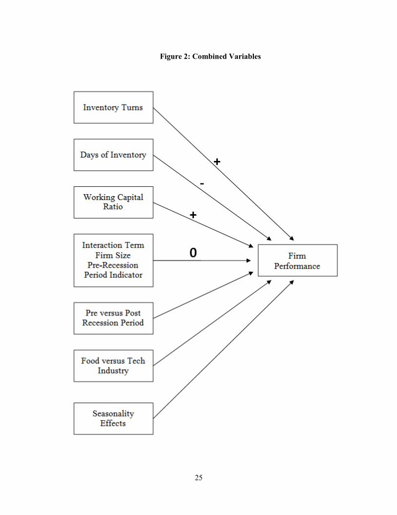
25
Figure 2: Combined Variables

26
inventory leanness (Eroglu & Hofer, 2011; Hofmann & Kotzab, 2010). Just-in-time theory,
when combined with a linear perspective of inventory leanness, frequently leads SC managers to
exploit these practices as managers lead their organization through a disruption to maintain firm
performance expectations (Goldsby, Griffis, & Roath, 2006; Huson & Nanda, 1995). Similarly,
earlier financial research presented evidence that suggests the greater the working capital, the
better the firm’s performance (Bierman, 1960), yet further research suggests that an optimal
range exists for working capital ratio (Emery & Cogger, 1982). Working capital requires
balance between a firm meeting current liabilities and greater asset utilization. In order to better
understand this differentiation, several new hypotheses stated below will attempt to tease out a
greater understanding of the relationship of leanness and slack resources while anticipating that
management will realize their favorable results during normal conditions and apply them to a
greater extent to drive performance due to the negative force from the economic disruption. As
stated earlier, this disruption created an inability for firms to expand and grow, corrections in
stock markets and the freezing of credit flows were some of the factors working against firms to
perform as they had during the prior economic growth period. The effects of this type of
disruption often forces firms to apply pressure across its supply chain to reduce costs and exploit
processes that can support “bottom line” financial improvement (Hendricks & Singhal, 2003).
Based on that premise, and with respect to the discussion above, the following hypotheses are
presented:
H2a. Days of inventory in the post-recession period should be lower than days of
inventory in the pre-recession period.
H2b. Inventory turns in the post-recession period should be higher than inventory turns
in the pre-recession period.

27
H3a. The variance of days of inventory in the pre-recession period will be greater than
the variance of days of inventory in the post-recession period.
H3b. The variance of inventory turns in the pre-recession period will be greater than the
variance of inventory turns in the post-recession period.
Hypothesis 2a states that days of inventory in the post-recession period should be lower
relative to the pre-recession period. Hypothesis 3a proposes that the variance of days of
inventory in the pre-recession period will be greater than the variance of days of inventory in the
post-recession period. The two hypotheses are similar insofar as both hypothesize greater
average days of inventory and greater days of inventory variance in the pre-recessionary period
relative to the post-recessionary period. Visually I see Hypothesis 2a and 3a as follows:
Hypothesis 2b states that inventory turns in the post-recession period should be higher relative to
the pre-recession period. Hypothesis 3b proposes that the variance of inventory turns in the pre-
recession period will be greater than the variance of inventory turns in the post-recession period.
The two hypotheses are similar insofar as both hypothesize greater average inventory turns and
greater inventory turns variance in the pre-recessionary period relative to the post-recessionary
period. Visually I see Hypothesis 2b and 3b as follows:
Thompson et al. (2009), Purdy (1967), and Galbraith (1973) see slack as a means to
provide inventories at the input (to absorb supplier delivery schedules) and output end (to absorb
Post-Recession
Days of Inventory
Pre-Recession
Days of Inventory
<
Post-Recession
Days of Inventory
Pre-Recession
Days of Inventory
>

28
fluctuations in demand). They posit that slack allows the supply to be less prone to interruption
and providing economic benefits to the firm in the long run. Yet, much of management and
administrative theory is preoccupied with eliminating slack through efficiency improvement and
optimization principles (Cyert & March, 1963b). Staw, Sandelands, and Dutton (1981) agree
with Cyert and March (1963) by demonstrating in their research that depleting slack can cause
rigidity and tightening of control tends to also diminish a firms financial performance and move
it closer to failure.
I argue that in a more prosperous economic period, e.g. a pre-recession period, slack
resources will be considered and implemented when firms have greater financial resources to
support slack in their strategic efforts. Conversely, in a declining economic period, e.g. a post-
recession period, firms will be eliminating slack resources to reduce costs or convert them into
performance enhancing activities due to pressure from the economic disruption (Daniel et al.,
2004). Therefore, the following hypothesis is proposed:
H4: The variance in working capital ratio in the pre-recession period will be greater
than the variance in working capital ratio in the post-recession period.
Visually I see hypothesis H4 as follows:
As mentioned earlier, prior research (Kuper, 2002) has proposed that larger firms
generally have access to resources (i.e., financing, inventory) which are not as available to
smaller firms and greater control over their competitive environment. Additionally, larger firms
may be able to afford slack resources, especially during normal periods (Garmestani et al., 2006).
> Post-Recession
Working Capital
Ratio Variance
Pre-Recession
Working Capital
Ratio Variance
>

29
Based on the definition of resilience as posited in this study, if smaller firms have less access to
resources and their survival becomes vulnerable, it is likely that their resilience will be affected
due to their size. This bias of smaller firms was eliminated by focusing only on firms with
annual revenue greater than $100 million. I follow Lev (1969) by identifying small firms as
having annual revenue less than $100 million. As firms become larger with greater control over
their competitive environment, their access to resources becomes greater (Garmestani et al.,
2006). Based on this premise, the largest firms within the large firm group should have greater
capability of managing their resources to withstand a disruption. Therefore, the following
hypothesis is proposed:
H5. The variance in firm performance in the pre-recessionary period will be less than the
variance in firm performance in the post-recessionary period.
I visually see hypothesis 5 as follows:
Regardless of firm size, the industry, degree of inventory leanness in a firm, or slack
resources I expect there to be significant variation among firm performance between the pre-
recession period and the post-recession period. Different firms have different resources and
capabilities, and this should lead to a high degree of heterogeneity in the ability of firms to adapt
and survive in response to a significant economic disruption (Rothaermel & Hill, 2005). I also
anticipate a wide degree of resilience among the firms. The range should be from non-existent to
a high degree of resilience within firms. If all firms were resilient, then they would not
experience a decline in firm performance in the post-recession period as compared to the pre-
recession period. This condition is highly unlikely since research demonstrates that, globally,
Post-Recession
Firm Performance
Pre-Recession
Firm Performance
<

30
supply chain resilience is lacking across many industries and organizations (Hendricks &
Singhal, 2005b); therefore, I anticipate less variance in firm performance in the pre-recession
period than in the post-recession period.
3.3 Summary
This chapter has established the research context for the study with a discussion of the
relationships between inventory leanness, slack resources, firm size, and firm performance
against a significant global economic disruption. A conceptual model was presented for the
study, and hypotheses have been developed and are summarized in Table 2.

31
Table 2: Summary of Hypotheses
Hypotheses
Number Hypotheses
H1a Inventory leanness (as measured by greater inventory turns) increases
resilience and therefore improves firm performance.
H1b Inventory leanness (as measured by lower days of inventory) increases
resilience and therefore improves firm performance.
H1c An increase in working capital ratio increases resilience and therefore
would lead to improved firm performance.
H1d Firm size in the pre-versus the post-recession has no effect on firm
performance between the pre-recession and the post-recession period.
H2a Days of inventory in the post-recession period should be lower than
days of inventory in pre-recession period.
H2b Inventory turns in the post-recession period should be higher than
inventory turns in the pre-recession period.
H3a
The variance of days of inventory in the pre-recession period will be
greater than the variance of days of inventory in the post-recession
period.
H3b The variance of inventory turns in the pre-recession period will be
greater than the variance of inventory turns in the post-recession period.
H4
The variance in working capital ratio in the pre-recession period will be
greater than the variance in working capital ratio in the post-recession
period.
H5
The variance in firm performance in the pre-recessionary period will be
less than the variance in firm performance in the post-recessionary
period.

32
4.0 RESEARCH METHODOLOGY AND DATA COLLECTION
This chapter describes the methods used for data collection and discussion of the research
design.
4.1 Research Design
Secondary data was collected from a data collection organization that included many
firms across two industries located across the globe to address the stated research questions. A
summary of the research design is provided in Table 3.
Table 3: Overview of Research Design
Area of
Concern Supply Chain
Research
Method Secondary Data Analysis
Unit of
Analysis The Firm
Data Source Publicly reported financial and operational data
Target Firms Food and Beverage, and Technology (consumer electronics and
computers) firms across the globe.
Industries
Included
Both low-and high-technology industries, such as food and beverage
(SIC 2000-2099), and computer and technology (SIC 3670-3679),
respectively.
4.2 Research Philosophy
The research method provides a foundation for advancing knowledge in any given
domain (Stone, 1978). Therefore, careful consideration is given in this study not only to
theoretical constructs, but also to the methodological approach. It should be noted that this
project follows the positivist research approach as the epistemological position (Myers, 2013).
To explore this particular area of research, secondary data are gathered to evaluate the
aforementioned hypotheses regarding the direct relationship of inventory leanness and slack

33
resources on the dependent variable of firm performance. Specifically, a quantitative approach
was applied to investigate the hypothesized relationships in the theoretical framework of
resilience.
4.3 Research Method
Ordinary Least Squares (OLS) regression, which is also known as multiple linear
regression, will be used to test hypotheses H1a through H1d. Multiple linear regression is used
when the dependent variable is continuous in nature and there are multiple independent variables
(Miles & Shevlin, 2001). Hypotheses 2a, 2b, 3a, 3b, 4 and 5 will be analyzed via an independent
samples t-test for differences in means. The use of an independent samples t-test is appropriate
when the dependent variable is continuous in nature and the independent variable is a
dichotomous nominal-level discrete variable (Ritchey, 2000). In addition, Levene’s test for
equality of variances will be used as a supplement to the independent samples t-test results.
4.4 Data Collection
Secondary data that is publically available was obtained from OneSource, Inc. through
Supply Chain Insights, LLC for the purpose of analysis of the aforementioned hypotheses.
Secondary data is well suited for studies designed to understand the present, investigate change,
and to examine phenomena comparatively (Jarvenpaa, 1991). The data collected for this project
will support the temporal aspect and provide the robustness to examine two industries and
hundreds of firms simultaneously. The research setting for this study is the manufacturing sector
of the global economy, as many of the firms in the dataset are multinational in scope. The data
are categorized by quarter (Q). The period of Q1, 2007 to Q3, 2008 represents the pre-recession
period, and the period Q1, 2010 to Q4, 2011 represents the post-recession period. Since the great
recession (which represents the disruption period in this study) was officially declared to have

34
begun in Q4, 2008 and then end in Q4, 2009 (Verick, 2010), these quarters have been eliminated
from the current analyses.
4.5 Data Preparation
Prior to all statistical analyses it was determined that said analyses should only be
conducted on companies that contained robust data. In other words, only companies that had
valid data points for all pre-recession and post-recession quarters under investigation were
included in the final dataset. In all there were 688 companies which had valid data for the seven
quarters of the pre-recession time period (Q1 of 2007 to Q3 of 2008) and the eight quarters of the
post-recession time period (Q1 of 2010 to Q4 of 2011). A total of 10,320 unique data points for
688 different companies are contained within the base dataset for these quarters.
As part of the procedure to ensure that only companies with robust data were used, a few
outlier observations (and the related observations from the same firm) were removed from the
data. For example, companies reporting return on assets greater than 100 percent (+/-) were
deleted from the dataset. It would be very rare for a company to have ROA greater than 100
percent, and it is more likely that the reporting of a ROA outside of this parameter was reported
in error. The removal of this faulty data resulted in the deletion of 19 companies (285
observations) from the base dataset. One of the companies in the dataset reported revenue of
-9.821 million for Q4 of 2007. It was decided that all observations for this company should be
removed from the dataset, since it is very rare for a company to have negative revenue. Thus the
final sample used for purposes of all data analyses was 10,020 unique data points for 668
different companies.

35
5.0 QUANTITATIVE ANALYSIS AND RESULTS
The chapter presents the analysis of the quantitative data obtained from the secondary
source. Section 5.1 presents the results for each of the hypotheses as they relate to each of the
constructs. The control variables were also included in the analysis to evaluate seasonality and
industry type. I used the SPSS Version 21 statistical application package to perform all data
analysis.
5.1 Results
In this section, I test each of the hypothesis associated with the conceptual model (see
Figure 1).
5.1.1 Hypotheses 1a - 1d. I argue that leanness and slack resources have an effect on
firm performance between the pre-recession and post-recession period when controlling for firm
size.
Hypotheses 1a through 1d are stated below:
H1a: Inventory leanness (as measured by greater inventory turns) increases resilience
and therefore improves firm performance.
H1b: Inventory leanness (as measured by lower days of inventory) increases resilience
and therefore improves firm performance.
H1c: An increase in working capital ratio increases resilience and therefore would lead
to improved firm performance.
H1d: Firm size in the pre-versus the post-recession has no effect on firm performance
between the pre-recession and the post-recession period.
Table 4 presents the means and standard deviations for all variables used in this
investigation. Several variables have been proxied as a way to concretely measure the concept

36
Table 4: Means and Standard Deviation for All Variables Used in Analysis
Variable Mean SD Mean SD Mean SD Mean SD Mean SD
Measure for Firm Size: Revenue by Value 585.65 2379.74 552.89 2267.57 614.33 2473.58 450.49 1441.40 1310.40 4927.32
Measure for Inventory Leanness: Days of Inventory 97.10 237.66 99.53 293.74 94.99 174.37 100.16 253.79 80.70 116.92
Measure for Inventory Leanness: Inventory Turns 8.86 14.01 8.97 14.81 8.76 13.26 8.87 13.97 8.81 14.23
Measure for Firm Performance: Return on Assets 0.05 0.10 0.04 0.10 0.05 0.10 0.05 0.10 0.30 0.11
Measure for Slack Resources: Working Capital Ratio 0.19 0.49 0.17 0.62 0.20 0.34 0.16 0.51 0.34 0.30
Variable Marking Pre or Post Recession Time Period (1=Post) 0.53 0.50 - - - - 0.53 0.50 0.53 0.50
Variable Marking Food or Tech Industry (1=Food) 0.84 0.36 0.84 0.36 0.84 0.36 - - - -
N=5,344N=4,676N=10,020 N=1,575N=8,445
Food and Beverage
Industries
Technology
IndustriesFull Dataset
Pre-Recessionary
Period
Post-Recessionary
Period
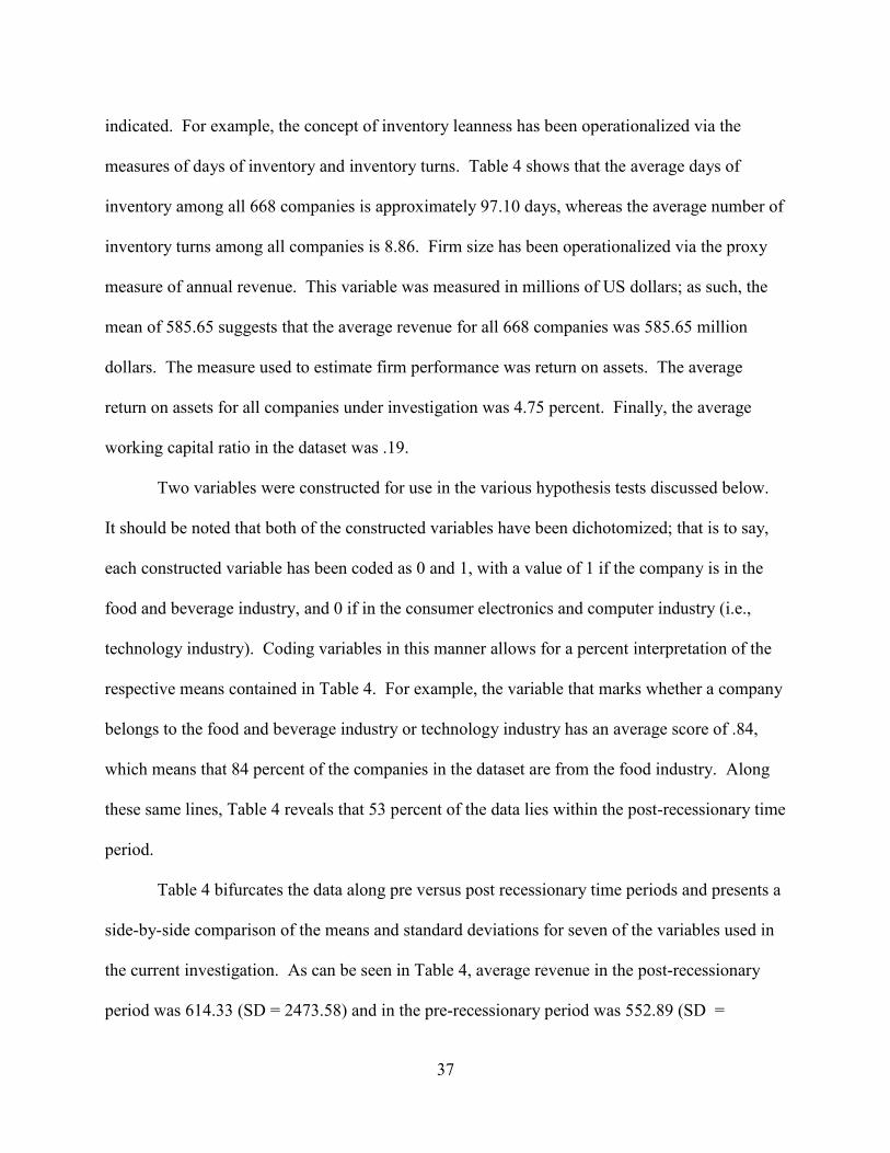
37
indicated. For example, the concept of inventory leanness has been operationalized via the
measures of days of inventory and inventory turns. Table 4 shows that the average days of
inventory among all 668 companies is approximately 97.10 days, whereas the average number of
inventory turns among all companies is 8.86. Firm size has been operationalized via the proxy
measure of annual revenue. This variable was measured in millions of US dollars; as such, the
mean of 585.65 suggests that the average revenue for all 668 companies was 585.65 million
dollars. The measure used to estimate firm performance was return on assets. The average
return on assets for all companies under investigation was 4.75 percent. Finally, the average
working capital ratio in the dataset was .19.
Two variables were constructed for use in the various hypothesis tests discussed below.
It should be noted that both of the constructed variables have been dichotomized; that is to say,
each constructed variable has been coded as 0 and 1, with a value of 1 if the company is in the
food and beverage industry, and 0 if in the consumer electronics and computer industry (i.e.,
technology industry). Coding variables in this manner allows for a percent interpretation of the
respective means contained in Table 4. For example, the variable that marks whether a company
belongs to the food and beverage industry or technology industry has an average score of .84,
which means that 84 percent of the companies in the dataset are from the food industry. Along
these same lines, Table 4 reveals that 53 percent of the data lies within the post-recessionary time
period.
Table 4 bifurcates the data along pre versus post recessionary time periods and presents a
side-by-side comparison of the means and standard deviations for seven of the variables used in
the current investigation. As can be seen in Table 4, average revenue in the post-recessionary
period was 614.33 (SD = 2473.58) and in the pre-recessionary period was 552.89 (SD =

38
2267.57). Days of inventory in the pre-recessionary period (M = 99.53; SD = 293.74) was not
significantly different than in the post-recessionary period (M = 94.99; SD = 174.37). Likewise,
inventory turns in the pre-recessionary period (M = 8.97; SD = 14.81) are not significantly
different than in the post-recessionary period (M = 8.76; SD = 13.26). Finally, the ratio between
food and beverage industries and technology industries is the same in both time periods (M =
.84; SD = .36), thus showing parity of the data.
There are only two statistically significant differences that exist within these means
between the pre- and post-recession period. Return on assets was slightly lower in the pre-
recessionary period (M = .04; SD = .10) than in the post-recessionary period (M = .05; SD =
.10). An independent samples t-test shows that the mean score for return on assets in the pre-
recessionary period is statistically lower than in the post-recessionary period (t = 2.638, df =
10,018, p < .01). Working capital ratio was also lower in the pre-recessionary period (M = .17;
SD = .62) than the post-recessionary period (M = .20; SD = .34). An independent samples t-test
also shows that working capital ratio is also statistically lower in the pre-recessionary period as
compared to the post-recessionary period (t = 2.837, df = 10,018, p < .01).
Table 4 also bifurcates the data along food and beverage industries versus technology
industries and presents a side-by-side comparison of the means and standard deviations for six of
the variables used in the current investigation. Statistically significant differences exist within
these means between the food and beverage industries and the technology industries for all
variables except inventory turns. Results of a series of independent samples t-tests showed that
return on assets (t = 6.428, df = 10,018, p < .001), revenue (t = 13.280, df = 10,018, p < .001) and
working capital ratio (t = 13.514, df = 10,018, p < .001) were all statistically significant for
technology industries as compared to food and beverage industries. In contrast, days of inventory

39
was statistically larger for the technology industries than for the food and beverage industries (t =
2.985, df = 10,018, p < .01).
In order to investigate the various aspects of Hypothesis 1 simultaneously, an Ordinary
Least Squares (OLS) regression was performed as the statistical modeling technique. The use of
regression is optimal when modeling two or more independent variables and one dependent
variable (Miles & Shevlin, 2001). Additionally, the standard errors were clustered at the firm
level. Without clustering the standard errors, correlations among variables might cause
misleading small standard errors and consequently narrow confidence intervals, larger t-
statistics, and low p-values (Miles & Shevlin, 2001). A regression without clustering of standard
errors was also performed; the results showed results similar to those obtained via the regressions
with the clustered standard errors. As such, the results with clustered standard errors are
presented in this chapter. Table 5 presents the results of the OLS regression of firm performance
as measured by return on assets on the six primary independent predictors of interest.
Variable B SE(B) p B SE(B) p B SE(B) p
Constant 2.118 0.375 *** 1.965 0.401 *** 2.020 0.402 ***
Inventory turns -0.002 0.007 -0.0004 0.017 -0.001 0.017
Days of inventory -0.002 0.001 *** -0.001 0.001 -0.001 0.001
Working capital ratio 2.417 0.231 *** 2.536 0.245 *** 2.535 0.245 ***
Firm size as measured by revenue by value 0.219 0.004 *** 0.223 0.044 *** 0.139 0.066 **
Pre versus post recession time period 0.447 0.207 * 0.430 0.207 * 0.345 0.213
Food and beverage versus technology 2.485 0.288 *** 2.491 0.288 *** 2.490 0.288 ***
Seasonal effects, Q1 -0.327 0.305 -0.339 0.305 -0.341 0.305
Seasonal effects, Q2 0.373 0.305 0.371 0.305 0.367 0.305
Seasonal effects, Q3 -0.246 0.305 -0.244 0.304 -0.244 0.304
Inventory turns, squared 0.0001 0.0001 0.000002 0.0001
Days of inventory, squared -0.00000001 0.000 -0.000001 0.000
Working capital ratio, squared -0.065 0.028 * -0.065 0.028 *
Interaction of pre versus post recession time period and firm size 0.147 0.087
R2
0.018 0.020 0.020 F 20.680 *** 16.777 *** 15.707 ***
Note: N=10,020, *=p<.05, **=p<.01, ***=p<.001, two-tailed tests.
Table 5: Unstandardized OLS Regression Coefficients Predicting Firm Performance as Measured by
Return on Assets
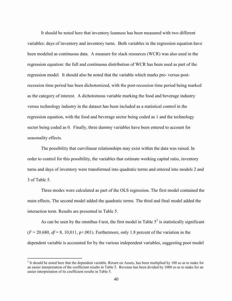
40
It should be noted here that inventory leanness has been measured with two different
variables: days of inventory and inventory turns. Both variables in the regression equation have
been modeled as continuous data. A measure for slack resources (WCR) was also used in the
regression equation: the full and continuous distribution of WCR has been used as part of the
regression model. It should also be noted that the variable which marks pre- versus post-
recession time period has been dichotomized, with the post-recession time period being marked
as the category of interest. A dichotomous variable marking the food and beverage industry
versus technology industry in the dataset has been included as a statistical control in the
regression equation, with the food and beverage sector being coded as 1 and the technology
sector being coded as 0. Finally, three dummy variables have been entered to account for
seasonality effects.
The possibility that curvilinear relationships may exist within the data was raised. In
order to control for this possibility, the variables that estimate working capital ratio, inventory
turns and days of inventory were transformed into quadratic terms and entered into models 2 and
3 of Table 5.
Three modes were calculated as part of the OLS regression. The first model contained the
main effects. The second model added the quadratic terms. The third and final model added the
interaction term. Results are presented in Table 5.
As can be seen by the omnibus f-test, the first model in Table 52 is statistically significant
(F = 20.680, df = 8, 10,011, p<.001). Furthermore, only 1.8 percent of the variation in the
dependent variable is accounted for by the various independent variables, suggesting poor model
2 It should be noted here that the dependent variable, Return on Assets, has been multiplied by 100 so as to make for
an easier interpretation of the coefficient results in Table 5. Revenue has been divided by 1000 so as to make for an
easier interpretation of its coefficient results in Table 5.
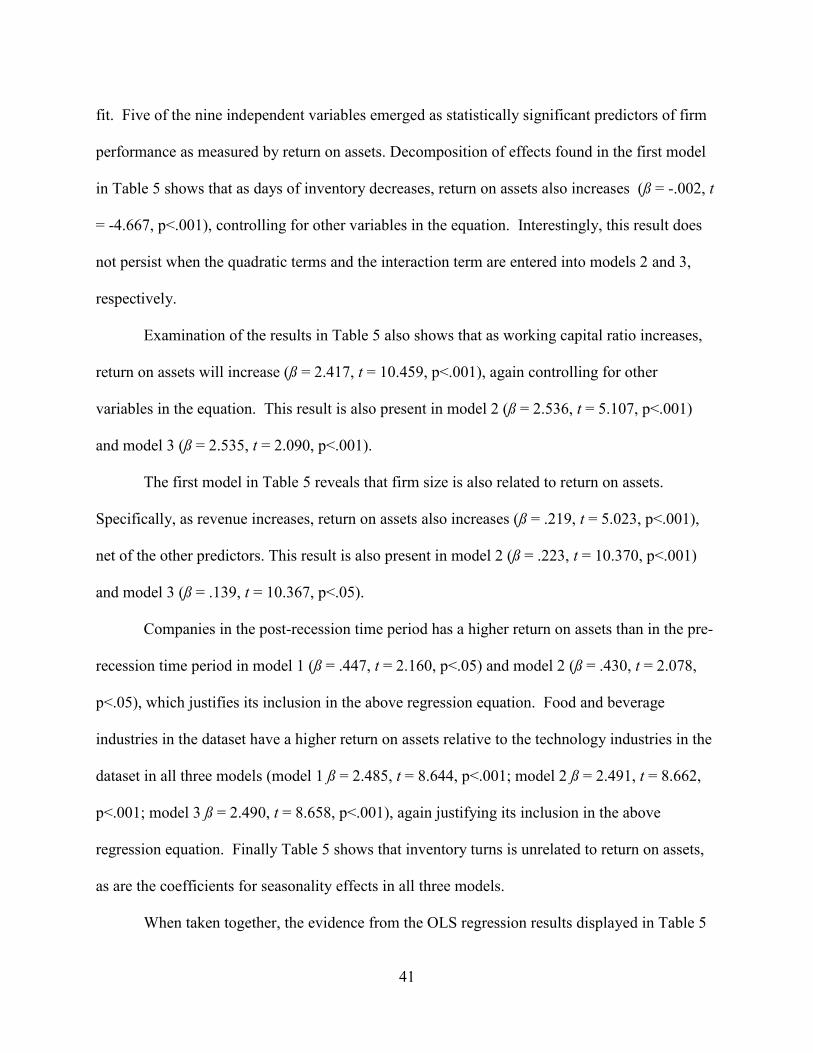
41
fit. Five of the nine independent variables emerged as statistically significant predictors of firm
performance as measured by return on assets. Decomposition of effects found in the first model
in Table 5 shows that as days of inventory decreases, return on assets also increases (ß = -.002, t
= -4.667, p<.001), controlling for other variables in the equation. Interestingly, this result does
not persist when the quadratic terms and the interaction term are entered into models 2 and 3,
respectively.
Examination of the results in Table 5 also shows that as working capital ratio increases,
return on assets will increase (ß = 2.417, t = 10.459, p<.001), again controlling for other
variables in the equation. This result is also present in model 2 (ß = 2.536, t = 5.107, p<.001)
and model 3 (ß = 2.535, t = 2.090, p<.001).
The first model in Table 5 reveals that firm size is also related to return on assets.
Specifically, as revenue increases, return on assets also increases (ß = .219, t = 5.023, p<.001),
net of the other predictors. This result is also present in model 2 (ß = .223, t = 10.370, p<.001)
and model 3 (ß = .139, t = 10.367, p<.05).
Companies in the post-recession time period has a higher return on assets than in the pre-
recession time period in model 1 (ß = .447, t = 2.160, p<.05) and model 2 (ß = .430, t = 2.078,
p<.05), which justifies its inclusion in the above regression equation. Food and beverage
industries in the dataset have a higher return on assets relative to the technology industries in the
dataset in all three models (model 1 ß = 2.485, t = 8.644, p<.001; model 2 ß = 2.491, t = 8.662,
p<.001; model 3 ß = 2.490, t = 8.658, p<.001), again justifying its inclusion in the above
regression equation. Finally Table 5 shows that inventory turns is unrelated to return on assets,
as are the coefficients for seasonality effects in all three models.
When taken together, the evidence from the OLS regression results displayed in Table 5

42
provide partial support for Hypothesis 1. Specifically, Hypothesis 1a stated that inventory
leanness (as measured by greater inventory turns) improves firm performance. There is no
evidence to support this hypothesis within the regression equations presented in Table 5.
Hypothesis 1b stated that inventory leanness (as measured by lower days of inventory) improves
firm performance. This hypothesis is supported by the evidence presented in the first regression
equation in Table 5. As days of inventory decreases, return on assets increases in the first model.
Hypothesis 1c states that an increase in working capital ratio would lead to improved firm
performance. This hypothesis is supported by the evidence within the regression equations
presented in Table 5. As working capital ratio increases, return on assets also increases in all
three models.
In order to investigate the tenets of Hypothesis 1d, an interaction term was created and
entered into the third model in Table 5. The interaction term between firm size and pre versus
post recessionary time periods is statistically non-significant. On the basis of this evidence it can
be concluded that there is no support for Hypothesis 1d. In other words, the data does not
support the contention that firm size differentially affects firm performance between the pre-
recession and the post-recession period.
As previously noted, the possibility of curvilinear effects concerning working capital
ratio, inventory turns and days of inventory was raised during the analysis phase of this project.
In order to account for this possibility, quadratic terms for each of the aforementioned variables
were entered into models 2 and 3. Results presented in Table 5 show that neither inventory turns
nor days of inventory were statistically related to the dependent variable. Working capital ratio
was negatively related to the dependent variable in model 2 (ß = -.065, t = -2.303, p<.05) and
model 3 (ß = -.065, t = -2.313, p<.05) of the equation set. As such, it can be concluded that

43
working capital ratio has a curvilinear relationship to return on assets.
The possibility that there could be variation in the data as a function of whether a
company was from the technology industries or from the food and beverage industries was raised
as a possibility. In order to investigate this possibility, the dataset was divided into its two
separate parts, and the regression analyses used to investigate Hypothesis 1 were re-estimated.
Tables 6a and 6b present the bifurcated data used to investigate Hypothesis 1. A difference in
the bifurcated data was found with respect to Hypothesis 1a. Specifically, the statistically
nonsignificant results found for hypothesis 1a for the full dataset was reversed when the data
were split between the technology companies and the food and beverage companies.
Among the food and beverage segment of the dataset, there was a significant and
negative relationship between inventory turns and return on assets, controlling for other factors
in the model. Interestingly, within the technology segment of the dataset, there was a significant
and positive relationship between inventory turns and return on assets, again controlling for other
Variable B SE(B) p B SE(B) p B SE(B) p
Constant 4.434 0.303 *** 4.507 0.338 *** 4.547 0.341 ***
Inventory turns -0.020 0.008 * -0.051 0.018 ** -0.051 0.018 **
Days of inventory -0.002 0.001 *** -0.001 0.001 -0.001 0.001
Working capital ratio 2.565 0.237 *** 2.697 0.252 *** 2.696 0.252 ***
Firm size as measured by revenue by value 0.124 0.076 0.139 0.076 0.053 0.122
Pre versus post recession time period 0.698 0.222 ** 0.685 0.222 ** 0.621 0.233 **
Seasonal effects, Q1 -0.086 0.327 -0.119 0.327 -0.123 0.327
Seasonal effects, Q2 0.721 0.327 * 0.704 0.327 * 0.700 0.327 *
Seasonal effects, Q3 0.003 0.327 -0.006 0.327 -0.007 0.327
Inventory turns, squared 0.00003 0.0001 * 0.00003 0.0001 *
Days of inventory, squared -0.00000001 0.000 -0.000001 0.000
Working capital ratio, squared -0.053 0.028 -0.054 0.028
Interaction of pre versus post recession time period and firm size 0.145 0.156
R2
0.017 0.020 0.020 F 18.399 *** 15.443 *** 14.226 ***
Note: N=10,020, *=p<.05, **=p<.01, ***=p<.001, two-tailed tests.
Table 6a: Unstandardized OLS Regression Coefficients Predicting Firm Performance as Measured by
Return on Assets, Food and Beverage Industries Only
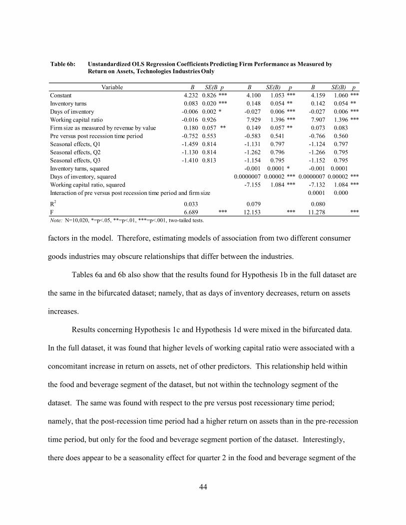
44
factors in the model. Therefore, estimating models of association from two different consumer
goods industries may obscure relationships that differ between the industries.
Tables 6a and 6b also show that the results found for Hypothesis 1b in the full dataset are
the same in the bifurcated dataset; namely, that as days of inventory decreases, return on assets
increases.
Results concerning Hypothesis 1c and Hypothesis 1d were mixed in the bifurcated data.
In the full dataset, it was found that higher levels of working capital ratio were associated with a
concomitant increase in return on assets, net of other predictors. This relationship held within
the food and beverage segment of the dataset, but not within the technology segment of the
dataset. The same was found with respect to the pre versus post recessionary time period;
namely, that the post-recession time period had a higher return on assets than in the pre-recession
time period, but only for the food and beverage segment portion of the dataset. Interestingly,
there does appear to be a seasonality effect for quarter 2 in the food and beverage segment of the
Variable B SE(B) p B SE(B) p B SE(B) p
Constant 4.232 0.826 *** 4.100 1.053 *** 4.159 1.060 ***
Inventory turns 0.083 0.020 *** 0.148 0.054 ** 0.142 0.054 **
Days of inventory -0.006 0.002 * -0.027 0.006 *** -0.027 0.006 ***
Working capital ratio -0.016 0.926 7.929 1.396 *** 7.907 1.396 ***
Firm size as measured by revenue by value 0.180 0.057 ** 0.149 0.057 ** 0.073 0.083
Pre versus post recession time period -0.752 0.553 -0.583 0.541 -0.766 0.560
Seasonal effects, Q1 -1.459 0.814 -1.131 0.797 -1.124 0.797
Seasonal effects, Q2 -1.130 0.814 -1.262 0.796 -1.266 0.795
Seasonal effects, Q3 -1.410 0.813 -1.154 0.795 -1.152 0.795
Inventory turns, squared -0.001 0.0001 * -0.001 0.0001
Days of inventory, squared 0.0000007 0.00002 *** 0.0000007 0.00002 ***
Working capital ratio, squared -7.155 1.084 *** -7.132 1.084 ***
Interaction of pre versus post recession time period and firm size 0.0001 0.000
R2
0.033 0.079 0.080
F 6.689 *** 12.153 *** 11.278 ***
Note: N=10,020, *=p<.05, **=p<.01, ***=p<.001, two-tailed tests.
Table 6b: Unstandardized OLS Regression Coefficients Predicting Firm Performance as Measured by
Return on Assets, Technologies Industries Only

45
dataset across all three models, but there is no support of an effect of seasonality on any other
quarter within F & B or the technology industries.
5.1.2 Hypothesis 2a and 3a. I argue that days of inventory in the post-recession period
should be lower than days of inventory in the pre-recession period, and that the variance of days
of inventory in the pre-recession period will be greater than the variance of days of inventory in
the post-recession period. Hypotheses 2a and 3a are stated below:
H2a: Days of inventory in the post-recession period should be lower than days of
inventory in the pre-recession period.
H3a: The variance of days of inventory in the pre-recession period will be greater than
the variance of days of inventory in the post-recession period.
In order to investigate this set of hypotheses, an independent samples t-test was
calculated for H2a, and a Levene’s test for equality of variances was calculated for H3a. The use
of an independent samples t-test and the Levene’s test is appropriate when the dependent
variable is continuous in nature and the independent variable is a dichotomous nominal-level
discrete variable (Ritchey, 2000). In this instance, days of inventory is being measured as a
continuous variable, and the variable which marks either the pre-recessionary or post-
recessionary time period has been dichotomized. Results of the independent samples t-test are
statistically nonsignificant (t= .954, df= 10,018, p>.05) and suggest that there is no relationship
between time period and days of inventory. Levene’s test for equality of variances is also
statistically nonsignificant (F =1.521, p>.05), which suggests that there is a nonsignificant
difference in the variance of days of inventory for the two time periods. Thus it can be concluded
that neither average days of inventory nor the variance associated with days of inventory are
significantly different between the pre-recession time period and the post-recession time period.
Hypotheses 2a and 3a are not supported by the data.

46
5.1.3 Hypotheses 2b and 3b. I argue that inventory turns in the post-recession period
should be higher than during the pre-recession period and variance of inventory turns in the pre-
recession period will be greater than the variance of inventory turns in the post-recession period.
Hypotheses 2b and 3b are stated below:
H2b. Inventory turns in the post-recession period should be higher than during the pre-
recession period.
H3b. The variance of inventory turns in the pre-recession period will be greater than the
variance of inventory turns in the post-recession period.
In order to investigate this set of hypotheses, an independent samples t-test was
calculated H2b, and a Levene’s test for equality of variances was calculated for H3b. The use of
an independent samples t-test and the Levene’s test is appropriate when the dependent variable is
continuous in nature and the independent variable is a dichotomous nominal-level discrete
variable (Ritchey, 2000). In this instance, inventory turns is being measured as a continuous
variable, and the variable which marks either the pre-recessionary or post-recessionary time
period has been dichotomized. Results of the independent samples t-test are statistically
nonsignificant (t= .776, df= 10,018, p>.05) and Levene’s test for equality of variances is also
statistically nonsignificant (F =3.662, p>.05). Thus it can be concluded that neither average
inventory turns nor the variance associated with inventory turns are significantly different
between the pre-recession time period and the post-recession time period. Hypotheses 2b and 3b
are not supported by the data.
The possibility that there could be variation in the data as a function of whether a
company was from the technology industries or from the food and beverage industries was again
raised as a possibility with respect to the tenets of Hypotheses 2a, 2b, 3a and 3b. In order to

47
investigate this possibility, the dataset was divided into its two separate parts, and the
independent samples t-tests and Levene’s test used to investigate the aforementioned hypotheses
were re-estimated. With respect to Hypotheses 2a, results of the independent samples t-test for
the food and beverage segment of the data (t= 1.217, df= 8,443, p>.05) and the technology
segment of the data (t= 1.225, df= 1,573, p>.05) are statistically nonsignificant. With respect to
Hypothesis H3a, the Levene’s test for the food and beverage segment of the data (F = 2.102,
p>.05) and the technology segment of the data (F = 0.780, p>.05) are also nonsignificant. Thus
it can be concluded that there is no relationship between time period and days of inventory as a
function of industry segment. Results of the independent samples t-test for the food and
beverage segment of the data (t= .436, df= 8,443, p>.05) and the technology segment of the data
(t= .936, df= 1,573, p>.05) are statistically nonsignificant for Hypotheses 2b. With respect to
Hypothesis 3b, the Levene’s test for the food and beverage segment of the data (F = 2.969,
p>.05) and the technology segment of the data (F = .835, p>.05) are also nonsignificant. Thus it
can be concluded that there is no relationship between time period and inventory turns as a
function of industry segment.
5.1.4 Hypothesis 4. I argue that the variance in working capital ratio in the pre-
recession period will be greater than the working capital ratio in the post-recession period.
Hypotheses 4 is stated below:
H4. The variance in working capital ratio in the pre-recession period will be greater than
the variance in the working capital ratio in the post-recession period.
In order to investigate this hypothesis, an equality of variances Levene’s test was
calculated. In this instance, WCR is being measured as a continuous variable, and the variable
which marks either the pre-recessionary or post-recessionary time period has been dichotomized.

48
Levene’s test for equality of variances is statistically significant (F =4.759, p<.05), which
suggests that there is a statistically significant difference in the variance of WCR for the two time
periods. Decomposition of the effects of the Levene’s test reveals that the variance of the WCR
for companies in the pre-recessionary time period (.382) is actually greater than the average
variance of the WCR for companies in the post-recessionary time period (.114), a result which
supports the tenets of Hypothesis 4. The evidence from the statistical analyses supports
Hypothesis 4.
The possibility that there could be variation in the data as a function of whether a
company was from the technology industry versus the food and beverage industry was again
raised as a possibility with respect to Hypothesis 4. In order to investigate this possibility, the
data were again bifurcated, and an equality of variance test (i.e., Levene’s test) was computed.
Results showed that the results for Hypothesis 4 are significant for the food and beverage
industries (F = 5.926, p < .05) only. No statistically significant result was found when the
dataset was restricted to technology industries (F = 1.324, p>.05) via the Levene’s test.
5.1.5 Hypothesis 5. I argue that as the variance in firm performance in the pre-
recessionary period will be less than the variance in firm performance in the post-recessionary
period. Hypothesis 1d is stated below:
H5. The variance in firm performance in the pre-recessionary period will be less than the
variance in firm performance in the post-recessionary period.
In order to investigate this hypothesis, a Levene’s test for equality of variance f-test was
calculated. The use of Levene’s test is appropriate when the dependent variable is continuous in
nature and the independent variable is a dichotomous nomial-level discrete variable (Miles &
Shevlin, 2001). In this instance, firm performance is being measured by return on assets, which

49
is a continuous variable. The variable that marks either the pre-recessionary or post-recessionary
time period has been dichotomized. Levene’s test for quality of variances is statistically
nonsignificant (F = .743, p>.05) in this instance. Therefore, Hypothesis 5 is not supported by
the data.
The possibility that there could be variation in the data as a function of whether a
company was from the technology industries versus the food and beverage industries was again
raised as a possibility with respect to Hypothesis 5. In order to investigate this possibility, the
data were again bifurcated. As was the case with the full dataset, Levene’s test for equality of
variances is again statistically nonsignificant (F = .317, p>.05) for the food and beverage
industries and the technology industries (F = .253, p>.05).
5.1.6 Determinants of firm performance in the post-recession period. Based on the
statistical results obtained via testing each of the five hypotheses, a post hoc analysis was
performed to further test supply chain resilience at the firm level, using the difference between
the pre-recession period firm performance (ROA) and post-recession period firm performance
(ROA) as the dependent variable. This additional analysis included collapsing independent
variables for the pre- and post-periods at the firm level and standardizing or centering the
variables to improve clarity of interpretation. Prior to this analysis it was suspected that DOI and
inventory turns may be creating multicollinearity. Variance inflation factors (VIF) for the
variable inventory turns in both pre and post periods were at 9.756 and 9.898, respectively.
According to Allison (1999), a VIF greater than 5 indicates that the variance of inventory turns
of the regression coefficient in increased due to collinearity. Therefore, multicollinearity exists
with this variable. Inventory turns was therefore eliminated in this regression in the post period.
Doing this resulted in a lowering of the VIF for all remaining variables to less than 2, which
50
eliminated the multicollinearity effect.
Table 7 includes the results of the additional analysis. These results show that the overall
model is statistically significant (F = 4.382, df = 7, 660, p<001). However, the coefficient of
determination revealed that only 4.4 percent of the variation in the dependent variable is
accounted for by the 7 independent variables, suggesting poor model fit. Two of the seven
variables emerged as statistically significant predictors of firm performance as measured by the
difference in return on assets in the post-versus the pre-recession period. Decomposition of
effects in Table 7 shows that as pre-period days of inventory increases, the difference in return
on assets between the pre and the post period increases (β = .004, t = 2.212, p<.05), controlling
for other variables in the equation. Examination of the results in Table 7 also shows that as pre-
period WCR increases, ROA in the post compared to the pre-recession period will decrease (β =
-2.688, t = -4.737, p<.001), again controlling for other variables in the equation. Also, Table 7
shows that firm size (β = .055, t = .498, p>.05), pre-period inventory turns (β = -.013, t = -.736,
p>.05), and post-period WCR (β = 1.404, t = 1.315, p>.05) are unrelated to the difference in the
pre- versus the post-period firm performance.
The evidence from the regression results in Table 7 provides a contrary perspective to the
commonly held position that greater inventory leanness or lower days of inventory will improve
firm performance, particularly in the post-recession period. Additionally, these regression results
show that a higher WCR prior to a disruption will decrease firm performance in the post-
recession time period. Higher WCR indicates that firms may not be efficiently utilizing their
excess cash and/or their current assets (Lev, 1969).

51

52
6.0 DISCUSSION AND IMPLICATIONS
In this section, I discuss the findings of this study and their implications. I also discuss
the contribution to theory and practice. I conclude my discussion with limitations and possible
future research opportunities.
6.1 Summary of Results and Discussion
In this study, I investigated the effect of inventory leanness and slack resources on firm
performance in light of the conditions of a global economic disruption. I also investigated if firm
resiliency is affected by inventory leanness and slack resources under conditions of this
economic disruption. To test this, I investigated the influence of inventory leanness on firm
performance by measuring the impact that days of inventory and inventory turns has on return on
assets. I also estimated the influence that slack resources has on firm performance by measuring
how working capital ratio impacts return on assets in the pre-recessionary period and the post-
recessionary period. I also investigated this influence between two industries that have different
supply chains. Choosing these industries provided the difference for comparison and contrasting
that was anticipated to support operationalizing the findings from the study among the consumer
goods categories. Finally, seasonality was investigated in the model due to the diverse demand
patterns and supply dynamics between the industries, as well as firm size due to the inherent
characteristic of size on a firm’s ability to weather disruptions. I argued that slack resources and
inventory leanness will positively influence firm performance as a firm maneuvers through an
economic disruption. I further argued that this positive influence should support supply chain
resiliency as a firm emerges from an economic disruption.
The literature review ties supply chain resiliency with how firms can build resiliency
capability, manage risk (i.e., identifying sources of risk, how those risks lead to consequences,

53
understand the drivers of risk, and formulate and implement strategies to mitigate risk), and
define the meaning of supply chain resilience, along with its benefits. However, I was not aware
of any studies that specifically assess the influence of the two primary SC constructs of inventory
leanness and slack resources. These twin SC constructs are critical to SC managers as they
maneuver through a global disruption that had immense consequences and widespread economic
decline not seen since the great depression and World War II era.
The study did not included data that was associated with the period defined as the great
recession (quarter 4 of 2008 to quarter 4 of 2009). The reason for eliminating the disrupted time
period was due to the stricter application of resilience adopted by this dissertation. The period
prior to the disruption represented a more normal state, and the time period after the disruption
represented a comparison to the “normal” state. If firms return to or are better than the normal
state performance after the disruption, then resilience is present. If firm performance is not equal
to or not better than the normal state, then resilience is not present. The normal state is
associated with an environment that is not experiencing a disruption or a decline. It is possible
that firms in this study could have been experiencing a disruption during the normal state or in
the recovery period after the economic recession. I did not include any other types of disruption
beyond the great recession period in this study.
Hypothesis 1a through 1d were structured to assess the effect of inventory leanness and
slack resources on firm performance. I controlled for industry and, where appropriate, tested for
differences in the effects by industry. I also controlled for seasonality. Seasonality often has an
effect on inventory and slack resources due to the impact seasonal aspects, such as the fourth
quarter holiday season, warm or cold weather influence on demand patterns, or raw material
availability due to seasonal harvests or availability. The findings for seasonality were minimal,

54
with only Q2 in the food and beverage industries showing an effect. No other quarters in the
food and beverage industries, or any quarter in the technology industries, supported seasonality
effects.
The hypothesis that inventory leanness would have a positive effect on firm performance
was partially supported. These results are mixed since hypothesis H1a, that increased inventory
turns would enhance firm performance, was not supported. In contrast, H1b, that increased days
of inventory would reduce firm performance, was supported. These findings are consistent with
Eroglu and Hofer (2011) and Demeter and Matyusz (2011), as it was found that industry type,
product type, demand or supply characteristics, and production technology will respond
differently to lean practices (Eroglu & Hofer, 2011). Further, leanness on firm performance is
mostly positive and generally non-linear. In most situations, inventory leanness is concave and
there is an optimal level of inventory leanness where the marginal effect of leanness on financial
performance becomes negative (Demeter & Matyusz, 2011). Slack resources effect on firm
performance was mixed between industries. Only within the food and beverage segment did an
increase in WCR show an effect on increased firm performance. The results of inventory
leanness on firm performance suggest that variations will occur depending on its position of the
curvilinear path. The results for an increase in WCR leading to improved performance (H1c) are
inconclusive in the literature on slack resources. In their meta-analysis of the slack-
performance relationship, Daniel et al. (2004) found that this relationship is more pronounced
when controlling for industry compared to those that do not. The current finding provides
additional empirical evidence for this industry specific relationship. In the current study, higher
levels of WCR increased firm performance, but this effect was not found for the technology
industry.

55
In Hypothesis 1d it was anticipated that firm size would decrease the variance in firm
performance between the pre- and post-recession periods. The findings for these two industries
did not support this hypothesis. This outcome is contrary to previous research (Garmestani et al.,
2006; Hendricks & Singhal, 2003). This opposite finding to the one hypothesized may be
specific to the industries selected, as industry specific results have been found with other
research in the lean and slack literature (Sharfman et al., 1988; Tan & Peng, 2003; Hambrick &
D´Aveni, 1988).
Inventory leanness, slack resources, time period, industry, and seasonality only accounted
for 1.8% (p<.001) of the variation in firm performance. However, when separated by industry,
these variables accounted for 1.7% (p<.001) in food and beverage and 3.3% (p<.001) in
technology sector of the variation in firm performance. Further examination of the results in
Table 7, found that as days of inventory and WCR increases, ROA also increases; additionally,
firms in the post-recession time period has higher ROA than in the pre-recession time period.
Food and beverage industry also have a higher ROA relative to the technology industry. Finally,
it was found that seasonality in the pre and post time periods within the industries was not
supported for the technology industry, although quarter 2 for the food and beverage supported a
seasonality effect. Again, it appears that seasonality is industry specific, but it is interesting that
seasonality was not a larger factor with these consumer goods industries that have demand
volatility that is highly influenced by events, weather, and supply availability.
Hypotheses 2a and 3a investigated the inventory leanness variables in the two time
periods. It was anticipated that in the pre-recessionary time period, which is the identified
normal or growth period, firms would have higher inventory with less turns to support
anticipated growth and expected demand based on historically based forecasts. These

56
hypotheses were supported by work done by Zsidisin and Wagner (2010) on supply chain risk
and resiliency. The results of the current analysis suggested that days of inventory does not have
a relationship with time period for these industries. Inventory turns in the post-recession period
were not significantly lower than in the pre-recession period (H2b) and the variance of inventory
turns in the pre-recession period was not greater than the variance of inventory turns in the post-
recession period (H3b), providing no evidence that firms had higher inventory during a period of
growth relative to a period of recovery post-recession. Thus, the results for the hypotheses set
H2 and H3 showed that inventory leanness is not significantly different between the two time
periods for either industry. As identified by Eroglu and Hofer (2011), the importance of
inventory leanness varies greatly from one industry to another. However, in this analysis I found
no support for the hypothesized relationship between inventory leanness and the economic
disruption in either industry.
The same investigation was performed with slack resources via the tenets of hypothesis 4
(variance in WCR in the pre-recession period will be greater than the WCR in the post-recession
period). The results were mixed for H4. Overall, the results support the hypothesis that there is
a relationship between WCR and time period. Yet when the data were bifurcated between the
food and beverage and technology industries, statistical significance was achieved for only the
food and beverage industries. Daniel et al. (2004) and Tan and Peng (2003) find similar
evidence that slack resources has a positive effect on firm performance during economic
transitions. Their studies, like this one, suggest that the slack – performance relationship may be
firm and/or industry specific.
In the case of variance in firm performance in the pre-recessionary period will be less
than the variance in firm performance in the post-recessionary period (H5), the results lie at odds

57
with the original hypothesis. It was anticipated that, controlling for firm size, the variance in
firm performance would be lower in the pre- than in the post-recession period. On the one hand,
recessionary forces have a pervasive impact on all segments of the economy and can have a
regressing to the mean effect on entire industries and economies (Blackhurst et al., 2011).
However, in this case it was anticipated that these forces would increase variance in firm
performance in the post time period. This assumption was based on the practical experience that
industries have gained with previous significant disruptions, the media reports that portrayed the
effects of this global disruption, and how a large portion of the literature on disruptions describes
the effects of disruptions on firm performance (Altay & Ramirez, 2010; Hambrick & D'Aveni,
1988; Jüttner, 2005; Kleindorfer & Saad, 2005; Tan & Peng, 2003). The opposite effect
occurred within the data used by this investigation. Firm performance variation was less in the
post-recessionary period as compared to the pre-recessionary period, a finding that aligns with
the work of Blackhurst et al. (2011). This finding may indicate that firms, especially large firms,
may be able to respond quickly to a disrupted condition by releasing available resources (e.g.,
downsizing employees, preexisting available credit) and converting available resources into
operating resources to minimize financial performance volatility (Daniel et al., 2004). Specific
to both the food and beverage and technology industries, firm size was not found in the current
study as a mechanism that decreased variance between the pre- and post-recession periods. Even
though conceptual studies suggest that firm size would have a decreasing effect, the present
results suggest that large firms may be able to rely on their size to overcome the effects on firm
performance as they encounter a disruption due to firm performance variation being less in the
post-recessionary period.
Table 8 summarizes the results of the hypothesis testing.

58
Table 8: Summary of Hypotheses Results
Hypothesis
Number Hypothesis Results
OverallFood and
BeverageTechnology
H1a
Inventory leanness (as measured by
greater inventory turns) increases
resilience and therefore improves firm
performance.
Not
SupportedSupported Supported
H1b
Inventory leanness (as measured by
lower days of inventory) increases
resilience and therefore improves firm
performance.
Supported SupportedNot
Supported
H1c
An increase in working capital ratio
increases resilience and therefore
would lead to improved performance.
Supported SupportedNot
Supported
H1d
Firm size in the pre- versus the post-
recession has no effect on firm
performance.
Not
Supported
Not
Supported
Not
Supported
H2a
Days of inventory in the post-recession
period should be lower than days of
inventory in the pre-recession period.
Not
Supported
Not
Supported
Not
Supported
H2b
Inventory turns in the post-recession
period should be higher than inventory
turns in the pre-recession period.
Not
Supported
Not
Supported
Not
Supported
H3a
The variance of days of inventory in
the pre-recession period will be
greater than the variance of days of
inventory in the post-recession period.
Not
Supported
Not
Supported
Not
Supported
H3b
The variance of inventory turns in the
pre-recession period will be greater
than the variance of inventory turns in
the post-recession period.
Not
Supported
Not
Supported
Not
Supported
H4
The variance in working capital ratio
in the pre-recession period will be
greater than the variance in working
capital ratio in the post-recession
period.
Supported SupportedNot
Supported
H5
The varinace in firm performance in
the pre-recessionary period will be
less than the variance in firm
perfornmance in the post-recessionary
period.
Not
Supported
Not
Supported
Not
Supported

59
6.2 Theoretical Contributions
This project investigated if a firm’s focus on inventory leanness and the availability of
slack resources have an effect on firm performance under conditions of an economic disruption.
As firms execute strategic plans, these two primary SC constructs are often instrumental in
determining how well a firm will perform throughout and after a major economic disruption.
The performance of a firm during and after a disruption is highly dependent on the degree of
resilience that exists within a firm prior to a disruption (Christopher & Peck, 2004). The
literature is silent on the interaction of inventory leanness and slack resources and their effect of
firm performance as it contributes to a firm’s resiliency under conditions of a financial
disruption, as was the case in the global great recession of 2008-2009. This study investigates
this critical interaction through empirical testing. The findings provide several implications for
theory.
Scholars have investigated many aspects of supply chain resilience and the relationships
of SC practices and risk-performance. Christopher and Peck (2004) and Pettit et al. (2010)
identified the components of a resilient SC and how to assess and apply those components.
Hendricks and Singhal (2003) identified the effect of disruptions on firm performance and
shareholder wealth, and Altay and Ramirez (2010) evaluated the impact of many different types
of disasters on different industries. Blackhurst et al. (2011) and Jüttner (2005) empirically
studied the effect of SC resilience against disruptions. None of this research, or for that matter
any other locatable studies, have examined SC practices of inventory leanness and slack
resources in the theoretical SC resiliency domain.
The inventory leanness – firm performance relationship has been studied as it relates to
how lean practices impact performance (Demeter & Matyusz, 2011) and how inventory leanness

60
mediates firm financial performance (Eroglu & Hofer, 2011). The slack resources – firm
performance relationship has been extensively researched in 66 separate studies that were
identified in the meta-analysis by Daniel et al. (2004); however, none of the studies included the
impact of slack resources on SC resilience measured against a significant global financial
disruption.
This research makes a theoretical contribution by extending resiliency theory with respect
to understanding the role of inventory leanness and slack resources and their effect on firm
performance toward supporting a firm’s supply chain resiliency. First, the study provides
additional depth to understanding the effect that inventory leanness and slack resources have on
firm performance relative to an economic disruption. This study used firms in two different
industry sectors, which provide us with information about how supply chain resiliency can be
affected. The current investigation took full advantage of a large secondary database with 15
quarters of data for 668 companies to analyze this relationship. By using ordinary least squares
regression analysis, I explained how inventory leanness and slack resources impact firm
performance in differing industries. The results indicate that inventory leanness does not support
firm performance relative to the technology and food and beverage industries; however, support
was demonstrated for the positive impact that slack resources will have on firm performance as
firms emerge from an economic disruption.
6.3 Contributions to Practice
Scholars and practitioners have investigated the effect of SC antecedents such as
inventory leanness and slack resources on firm performance (Pettit et al., 2010; Ponomarov &
Holcomb, 2009; Sharfman et al., 1988; Williams, 2011). However, these scholars and
practitioners have not evaluated these crucial processes under conditions of an economic

61
disruption, and the impact that said disruption will have on supply chain resiliency. The original
research questions in the study have been addressed with mixed results. The positive influence
of inventory leanness on firm performance is supported, but it is industry specific, and the pre- or
post-recession period does not seem to perturb inventory leanness. Thus, even though inventory
leanness may support firm performance for a particular industry, there is no support that it makes
a difference between the pre and post disruptive time periods. The positive influence of slack
resources is similar to inventory leanness. Slack supports firm performance, but it is industry
specific, as slack resources are a factor among food and beverage industries, but not for the
technology industry. In contrast to inventory leanness, slack resources make a difference in firm
performance between pre and post-disruptive time periods. WCR is greater in the pre disruption
period. This increase in a more stable growth period has been supported in other research
(Sharfman et al., 1988; Daniel et al., 2004). This greater level of slack resources during the pre-
disruptive period could also lead to less variation in firm performance during the disruption, and
that a higher level of firm performance in the post time period leads to the “unlocking” or
converting of slack into performance enhancing activity (Daniel et al., 2004). Industries that
have more volatile demand patterns, short product life cycles, longer and more global supply
chains, such as those in the technology sector, may not respond as positively to the presence of
slack resources. Additionally, it was found that within these two industries, largeness of the firm
may not be a universal antidote for encountering a disruption, but may support recovery with less
variation in the post-recession period.
In this study it was anticipated that firm performance variation would be greater in the
post-disruptive period as compared to the pre-disruptive time period simply due to the pressure
associated with the disruption. The results supported a contrary view and may be due to factors

62
that were not accounted for in the predictive models estimated in the current study. There are
many factors beyond the scope of this research that could contribute to such a finding, such as
greater volatility in forecasting demand or greater innovation introduction into the marketplace
during the pre-period. From a resiliency perspective, in the post-period, firms will often exploit
resources and lean processes to support firm performance expectations. In other words, firms
will become “lean and mean” to control costs, or convert resources, such as cash reserves, excess
inventories or supplier relationships directed to supporting firm performance (Womack & Jones,
2010). With greater focus by the firms in the post-recessionary period on controlling costs and
managing the business more tightly, it is the case that firm performance across industries will
have less variation than what I typically see in a growth or more normal economy.
The current research provides a valuable contribution to the practice of supply chain
management and resiliency by offering a better understanding of how inventory leanness and
slack resources can affect firm performance in the face of a disruption within their respective
industry. This research also provides a framework for firms to historically assess how their
inventory leanness and slack resources within their supply chain responded to the great recession
disruption and determine if their firm’s resiliency was sufficient to emerge at or greater than their
pre-disrupted firm performance level. The results of their assessment should lend insight toward
how SC managers can evaluate their processes and make course corrections to their firm’s
strategic initiatives to become more prepared for the next, inevitable disruption.
6.4 Limitations of the Study
There are several limitations associated with the current study, the first of which is
related to the selected definition of supply chain resilience. The literature on this topic is mixed.
Some scholars see SC resilience as an ability to rebound from unexpected, adverse situations and

63
to return where they left off (Christopher & Peck, 2004), while others see SC resilience beyond
restoring operations to include emerging from the disruption to a more competitive state with
greater capabilities (Sheffi, 2005). This study adopts the former definition that narrows
resilience to a firm returning to the financial performance they experienced before the disruption
or to a greater level, but it is not necessary to be at a more competitive state with greater
capabilities post the disruption to have resiliency. Also, this study only includes two industries
and is limited to firms with greater than 100 million US dollars in annual revenue. The inclusion
of additional industries and firms may provide different empirical results that may not support
the findings that are specific to the large firms within the two industries selected.
Firm size based on annual revenue was found to be a nonsignificant predictor between
the pre period and the post period in the overall results. Intuitively, based on an economic
disruption of the magnitude encountered in the great recession, it was anticipated that a
significant difference between the periods would emerge in the data. Several post hoc analyses
were performed to investigate this question, including the results from Table 7, and each analysis
with the current dataset provided nonsignificant results regarding differences between periods.
The statistically nonsignificant results with respect to firm size could be the result of
spuriousness and/or the failure to control for a robust number of additional independent
predictors. The application of a longitudinal or panel data analysis where the variables are
observed overtime with different time periods, and the inclusion of additional variables could
enhance the explanatory power of a model (Frees, 2004). Additionally, this study used quarterly
data for the pre- and post-recession periods across all firms. Therefore, I assumed that all firms
are homogenous and there is no individual firm effect. A future research opportunity could
apply a panel analysis to tease out the individual firm effects pre and post a disruption to

64
measure the effect on supply chain resilience.
Secondary data was used for this project. There is a concern that is inherent to the use of
secondary data by this project that future researchers may wish to address. Many of the
companies in the current dataset are international and are governed by different reporting
requirements. Although I am confident that the data is consistent for each of the firms and that
every effort was made by the supplier of the data (OneSource, Inc.) to insure consistency in the
data, it may be the case that there were differences within the dataset that could not be detected.
Additionally, the limited number of variables that examine leanness and slack beyond
inventories and WCR may have lent to the poor fit (R square of less than 5 percent) in the
regression models that were used to test the tenets of Hypothesis set 1. That is to say, the proxies
used to operationalize the various concepts in the current investigation (i.e., firm size, WCR,
etc.) may not have been robust. That said, it should be noted that when accessing global data
across multiple years and industries, robust data is limited. The variables selected were well
supported in the literature and the data was thoroughly examined for accuracy. In other words,
the best available data was used to investigate the hypotheses associated with this project.
Additional ad hoc analysis highlighted conflicting results in the effect of DOI and WCR
on firm performance in both pre and post periods. These results may be due to an undetected
and latent interaction between DOI and WCR as WCR has both inventory and assets as a
component of its ratio. Specifically, WCR has current assets as a component of the numerator of
the ratio with current assets including accounts receivables, prepaid expenses, securities, cash,
and inventory. However, WCR is often used as a proxy for measuring slack in much of the slack
resource–firm performance relationship literature (Daniel et al., 2002). Nevertheless, future
65
researchers should consider other slack variables as a substitute for WCR, such as debt/equity
ratio or administrative expense/cost of goods sold ratio.
The data available was at the firm level which was applied for inferring supply chain
performance and limits the focus of this study to an indirect investigation of supply chain
resilience. Specifically, ROA was the variable for determining performance. Future research
could identify a more direct measure of supply chain resilience, e.g. the rate of recovery from
sudden performance decline to a prior state of performance, or some sort of stability index
despite an economic disruption.
6.5 Future Research
This study only investigated two primary supply chain practices, inventory leanness and
slack resources associated with firm performance in an economically disrupted environment.
This relationship between inventory leanness and slack resources was only studied during the
great recession period of 2008-2009 across two industries. There are many other types of
disruptions that can affect firm performance across other industries (Wagner & Bode, 2006).
Also, there are other SC practices that managers can implement to support a firm’s resiliency in
preparing for and combating a disruption (Pettit et al., 2010). There are numerous opportunities,
both quantitatively and qualitatively, based on the permutations that exist outside this study
between type of industry, firm size, type of disruption, type of SC practice, measurement
techniques, and capabilities assessment for additional studies. Future researchers may wish to
consider these issues as they implement their own investigations.
Some additional research questions that could be investigated by future researchers based
on the above opportunities could include:

66
1. Why do industries differ in their performance as they maneuver through a disruption?
2. Are SC principles or practices complimentary or do they create tension as firms build SC
resilience? More specifically, how should firms value holding inventory (leanness)
versus holding cash (slack resources) as a firm builds resilience?
3. How do attitude and risk perception of SC managers influence focus on leanness and
slack resources under conditions of an economic disruption?
Historically, over the past century since the post Fredrick Taylor scientific management
era, numerous disruptive events such as world wars, a great depression, “9/11”, Hurricane
Katrina, and the great recession, (to name a few) have threatened a firm’s survival. A recent
study by Sheffi (2005) found that most companies are not strategically considering how to
systematically manage resilience. Understanding and building SC resilience characteristics into
a firm will support the ability of a firm to defend the next inevitable disruption and provide the
ability to adapt and thrive in the long-term. Increasing our understanding of supply chain
resilience will prove to be the ultimate competitive advantage in an age of increasing complexity
and turbulence.

67
BIBLIOGRAPHY
Agarwal, A., Shankar, R., & Tiwari, M. K. (2006). Modeling the metrics of lean, agile and
leagile supply chain: An ANP-based approach. European Journal of Operational
Research, 173(1), 211-225.
Altay, N., & Ramirez, A. (2010). Impact of disasters on firms in different sectors: implications
for supply chains. Journal of Supply Chain Management, 46(4), 59-80.
Beamon, B. M. (1999). Measuring supply chain performance. International Journal of
Operations & Production Management, 19(3), 275-292.
Beck, T., Demirgüç-Kunt, A., & Maksimovic, V. (2005). Financial and Legal Constraints to
Growth: Does Firm Size Matter? The Journal of Finance, 60(1), 137-177.
Bierman, H., Jr. (1960). Measuring Financial Liquidity. Accounting Review, 35(4), 628-632.
Blackhurst , J., Craighead, C. W., Elkins, D., & Handfield, R. B. (2005). An empirically derived
agenda of critical research issues for managing supply-chain disruptions. International
Journal of Production Research, 43(19), 4067-4081.
Blackhurst, J., Dunn, K. S., & Craighead, C. W. (2011). An empirically derived framework of
global supply resiliency. Journal of Business Logistics, 32(4), 374-391.
Bourgeois, L. J. (1981). On the measurement of organizational slack. Academy of Management
review, 6(1), 29-39.
Cecere, L. M., & Chase Jr., C. W. (2013). Bricks Matter: The Role of Supply Chains in Building
Market-Driven Differentiation. Hoboken, NJ: John Whiley & Sons, Inc.
Chen, I. J., & Paulraj, A. (2004). Towards a theory of supply chain management: the constructs
and measurements. Journal of Operations Management, 22(2), 119-150.

68
Chen, L., & Miller-Hooks, E. (2012). Resilience:An Indicator of Recovery Capability in
Intermodal Freight Transport. Transportation Science, 46(1), 109-123.
Cheng, J. L., & Kesner, I. F. (1997). Organizational slack and response to environmental shifts:
The impact of resource allocation patterns. Journal of Management, 23(1), 1-18.
Cho, S., Mathiassen, L., & Robey, D. (2006). Dialectics of resilience: a multi-level analysis of a
telehealth innovation. Journal of Information Technology, 22(1), 24-35.
Christopher, M., & Holweg, M. (2011). “Supply Chain 2.0”: managing supply chains in the era
of turbulence. International Journal of Physical Distribution & Logistics Management,
41(1), 63-82.
Christopher, M., & Peck, H. (2004). Building the resilient supply chain. International Journal of
Logistics Management, 15(2), 1-13.
Cooper, R., & Maskell, B. H. (2008). How to manage through worse-before-better. MIT Sloan
Management Review, 49(4), 58-65.
Cyert, R. M., & March, J. (1963a). A behavioral theory of the firm. University of Illinois at
Urbana-Champaign's Academy for Entrepreneurial Leadership Historical Research
Reference in Entrepreneurship.
Cyert, R. M., & March, J. G. (1963b). A behavioral theory of the firm. Englewood Cliffs, NJ, 2.
Daniel, F., Lohrke, F. T., Fornaciari, C. J., & Turner Jr, R. A. (2004). Slack resources and firm
performance: a meta-analysis. Journal of Business Research, 57(6), 565-574.
Demeter, K., & Matyusz, Z. (2011). The impact of lean practices on inventory turnover.
International Journal of Production Economics, 133(1), 154-163.

69
Dullaghan, A., Harcourt, E., McCarthy, M., & Raftery, D. (2001). Improving efficiencies in
product discontinuation Developed for the Grocery Manufacturers Association by Prime
Consulting Group, 1-29.
Ellis, S. C., Shockley, J., & Henry, R. M. (2011). Making sense of supply disruption risk
research: A conceptual framework grounded in enactment theory. Journal of Supply
Chain Management, 47(2), 65-96.
Emery, G. W., & Cogger, K. O. (1982). The Measurement of Liquidity. Journal of Accounting
Research, 20(2), 290-303.
Eroglu, C., & Hofer, C. (2011). Lean, leaner, too lean? The inventory-performance link revisited.
Journal of Operations Management, 29(4), 356-369.
Fama, E. F., & French, K. R. (1989). Business conditions and expected returns on stocks and
bonds. Journal of financial economics, 25(1), 23-49.
Fullerton, R. R., & McWatters, C. S. (2001). The production performance benefits from JIT
implementation. Journal of Operations Management, 19(1), 81-96.
Fullerton, R. R., McWatters, C. S., & Fawson, C. (2003). An examination of the relationships
between JIT and financial performance. Journal of Operations Management, 21(4), 383-
404.
Galbraith, J. K. (2009). Who Are These Economists, Anyway? Thought & Action, 85, 85-97.
Galbraith, J. R. (1973). Designing complex organizations: Addison-Wesley Longman Publishing
Co., Inc.
Garmestani, A. S., Allen, C. R., Mittelstaedt, J. D., Stow, C. A., & Ward, W. A. (2006). Firm
size diversity, functional richness, and resilience. Environment and Development
Economics, 11(4), 533-551.

70
Gertler, M., & Gilchrist, S. (1994). Monetary policy, business cycles, and the behavior of small
manufacturing firms. The Quarterly Journal of Economics, 109(2), 309-340.
Gittell, J. H. (2008). Relationships and Resilience Care Provider Responses to Pressures From
Managed Care. The Journal of Applied Behavioral Science, 44(1), 25-47.
Goldsby, T. J., Griffis, S. E., & Roath, A. S. (2006). Modeling lean, agile, and leagile supply
chain strategies. Journal of Business Logistics, 27(1), 57-80.
Grusky, D. B., Western, B., & Wimer, C. (2011). The great recession: Russell Sage Foundation.
Hambrick, D. C., & D'Aveni, R. A. (1988). Large Corporate Failures as Downward Spirals.
Administrative Science Quarterly, 33(1), 1-23.
Hendricks, K. B., & Singhal, V. R. (2003). The effect of supply chain glitches on shareholder
wealth. Journal of Operations Management, 21(5), 501-522.
Hendricks, K. B., & Singhal, V. R. (2005b). An Empirical Analysis of the Effect of Supply
Chain Disruptions on Long-Run Stock Price Performance and Equity Risk of the Firm.,
14: 35–52. Production and Operations Management, 14, 35-52.
Hofer, C., Eroglu, C., & Rossiter Hofer, A. (2012). The effect of lean production on financial
performance: The mediating role of inventory leanness. International Journal of
Production Economics, 138(2), 242-253.
Hofmann, E., & Kotzab, H. (2010). A suppply chain-oriented approach of working capital
management. Journal of Business Logistics, 31(2), 305-330.
Horne, J. F. (1997). The coming age of organizational resilience. Paper presented at the
BUSINESS FORUM-LOS ANGELES-.
Huson, M., & Nanda, D. (1995). The impact of just-in-time manufacturing on firm performance
in the US. Journal of Operations Management, 12(3–4), 297-310.

71
Inman, R. A., & Mehra, S. (1993). Financial justification of JIT implementation. International
Journal of Operations & Production Management, 13(4), 32-39.
Jarvenpaa, S. L. (1991). Panning for gold in information systems research: second-hand data.
Information Systems Research: Contemporary Approaches and Emergent Traditions, 63-
80.
Jayaram, J., Vickery, S., & Droge, C. (2008). Relationship building, lean strategy and firm
performance: an exploratory study in the automotive supplier industry. International
Journal of Production Research, 46(20), 5633-5649.
Jensen, M. C. (1986). Agency costs of free cash flow, corporate finance, and takeovers. The
American economic review, 323-329.
Jones, D. T., Roos, D., & Womack, J. P. (1990). Machine that Changed the World: Simon and
Schuster.
Jüttner, U. (2005). Supply chain risk management: Understanding the business requirements
from a practitioner perspective. The International Journal of Logistics Management,
16(1), 120-141.
Ketchen, D. J., Rebarick, W., Hult, G. T. M., & Meyer, D. (2008). Best value supply chains: A
key competitive weapon for the 21st century. Business Horizons, 51(3), 235-243.
Kleindorfer, P. R., & Saad, G. H. (2005). Managing disruption risks in supply chains. Production
and Operations Management, 14(1), 53-68.
Kuper, A. (2002). Hardening vulnerable links in the supply chain. TOTALsupplychain, February,
1-4.
Kurawarwala, A. A., & Matsuo, H. (1996). Forecasting and inventory management of short life-
cycle products. Operations Research, 44(1), 131-150.

72
Latham, S., & Braun, M. (2011). Economic recessions, strategy, and performance: a synthesi.
Journal of Strategy and Management, 4(2), 96-115.
Lengnick-Hall, C. A., Beck, T. E., & Lengnick-Hall, M. L. (2011). Developing a capacity for
organizational resilience through strategic human resource management. Human
Resource Management Review, 21(3), 243-255. doi: 10.1016/j.hrmr.2010.07.001
Lev, B. (1969). Industry averages as targets for financial ratios. Journal of Accounting Research,
290-299.
Levy, D. L. (1997). Lean production in an international supply chain. Sloan management review,
38, 94-102.
Lewis, M. A. (2000). Lean production and sustainable competitive advantage. International
Journal of Operations & Production Management, Vol. 20(Iss: 8), 959 - 978
Lux, T., & Westerhoff, F. (2009). Economics crisis. Nat Phys, 5(1), 2-3.
Mandal, S. (2012). An Empirical Investigation into Supply Chain Resilience. The IUP Journal of
Supply Chain Management, 9(4), 46-61.
Marino, K. E., & Lange, D. R. (1983). Measuring organizational slack: a note on the
convergence and divergence of alternative operational definitions. Journal of
Management, 9(1), 81-92.
Martin-Breen, P., & Anderies, J. M. (2011). Resilience: A Literature Review. (Department of
Philosophy, CUNY Graduate Center, New York, NY).
Miles, J., & Shevlin, M. (2001). Applying regression and correlation: A guide for students and
researchers: Sage.
73
Montiel, P. J. (2011). On Macroeconomic Reforms and Macroeconomic Resiliency: Lessons
from the Great Recession. Modern Economy, 02(04), 528-537.
Myers, M. D. (2013). Qualitative research in business and management. Thousand Oaks, CA:
Sage.
Ou, C. S., Liu, F. C., Hung, Y. C., & Yen, D. C. (2010). A structural model of supply chain
management on firm performance. International Journal of Operations & Production
Management, 30(5), 526-545.
Pettersen, J. (2009). Defining lean production: some conceptual and practical issues. The TQM
Journal, 21(2), 127-142.
Pettit, T. J., Fiksel, J., & Croxton, K. L. (2010). Ensuring supply chain resilience: development
of a conceptual framework. Journal of Business Logistic, 31(1), 1-21.
Ponis, S. L. (2012). Supply chain resilience: Definition of concept and its formative elements.
The Journal of Applied Business Research, 28(5), 921-929.
Ponomarov, S. Y., & Holcomb, M. C. (2009). Understanding the concept of supply chain
resilience. The International Journal of Logistics Management, 20(1), 124-143.
Purdy, L. R. (1967). Organizational conflict: Concepts and models. Administrative Science
Quarterly.
Raisch, S., & Birkinshaw, J. (2008). Organizational ambidexterity: Antecedents, outcomes, and
moderators. Journal of Management, 34(3), 375-409.
Rao, S., & Goldsby, T. J. (2009). Supply chain risks: a review and typology. International
Journal of Logistics Management, The, 20(1), 97-123.
Reinmoeller, P., & Van Baardwijk, N. (2005). The link between diversity and resilience. MIT
Sloan Management Review, 46(4), 61.

74
Ritchey, F. J. (2000). The statistical imagination: Elementary statistics for the social sciences:
McGraw-Hill.
Rothaermel, F. T., & Alexandre, M. (2008). Ambidexterity in Technology Sourcing: The
Moderating Role of Absorptive Capacity. Organization Science, 20(4), 759-780.
Rothaermel, F. T., & Hill, C. W. (2005). Technological discontinuities and complementary
assets: A longitudinal study of industry and firm performance. Organization Science,
16(1), 52-70.
Sharfman, M. P., Wolf, G., Chase, R. B., & Tansik, D. A. (1988). Antecedents of organizational
slack. Academy of Management review, 13(4), 601-614.
Sheffi, Y. (2005). Building a resilient supply chain. Harvard Business Review Supply Chain
Strategy, 1(5), 1-4.
Singh, J. V. (1986). Performance, Slack, and Risk Taking in Organizational Decision Making.
The Academy of Management Journal, 29(3), 562-585. doi: 10.2307/256224
Småros, J., Lehtonen, J.-M., Appelqvist, P., & Holmström, J. (2003). The impact of increasing
demand visibility on production and inventory control efficiency. International Journal
of Physical Distribution & Logistics Management, 33(4), 336-354.
Staw, B. M., Sandelands, L. E., & Dutton, J. E. (1981). Threat-rigidity effects in organizational
behavior: A multilevel analysis. Administrative Science Quarterly, 26(4).
Stone, E. F. (1978). Research methods in organizational behavior: Goodyear Publishing
Company, Santa Monica, CA.
Supply Chain Resilience. (November, 2012). CIP and Business Continuity Institute(4th annual
survey).

75
Tan, J., & Peng, M. W. (2003). Organizational slack and firm performance during economic
transitions: Two studies from an emerging economy. Strategic Management Journal,
24(13), 1249-1263.
Thompson, J. D., Scott, W. R., & Zald, M. N. (2009). Organizations in action: Social science
bases of administrative theory: Transaction Books.
Verick, S. I., I. (2010). The great recession of 2008 - 2009: Causes, consequences and policy
responses. Discussion paper series // Forschungsinstitut zur Zukunft der Arbeit,, No.
4934.
Wagner, S. M., & Bode, C. (2006). An empirical investigation into supply chain vulnerability.
Journal of Purchasing and Supply Management, 12(6), 301-312.
Wagner, S. M., & Bode, C. (2008). An empirical examination of supply chain performance along
several dimensions of risk. Journal of Business Logistics, 29(1), 307-325.
Wagner, S. M., Grosse-Ruyken, P. T., & Erhun, F. (2012). The link between supply chain fit and
financial performance of the firm. Journal of Operations Management, 30(4), 340-353.
Wagner, S. M., & Neshat, N. (2010). Assessing the vulnerability of supply chains using graph
theory. International Journal of Production Economics, 126(1), 121-129.
Williams, J. A. (2011). An Analysis of School Business Practices to Increase available Slack
Resources for Contingencies and Other Management Concerns. Unita Country School
District, 1, 1-28.
Womack, J. P., & Jones, D. T. (2010). Lean Thinking: Banish Waste and Create Wealth in Your
Corporation. New York, NY: SimonandSchuster. com.
Wu, C., & Ho, S.-J. (1997). Financial Ratio Adjustment: Industry-Wide Effects or Strategic
Management. Review of Quantitative Finance and Accounting, 9(1), 71-88.
76
Zsidisin, G. A., & Wagner, S. M. (2010). Do perceptions become reality? The moderating role of
supply chain resiliency on disruption occurrence. Journal of Business Logistics, 31(2), 1-
20.