the impact of interest rate risk-taking on a bank's...
TRANSCRIPT

UNIVERSITY OF TWENTE
MASTER’S THESIS
The impact of interest raterisk-taking on a bank’s
profitabilityA new dimension to balance sheet improvement
Author:T. ROEBERS
Supervisors:B. ROORDA (UT)R. JOOSTEN (UT)
D. FOKKEMA (EY)P. VERSTAPPEN (EY)
A thesis submitted in fulfillment of the degree of Master of Science
in
Financial Engineering and Management
May 25, 2017


iii
AbstractWith term premia present in the yield curve, banks have incentives to
create mismatches between term structures of cash flows and with this, ex-pose themselves to interest rate risk. Especially in the current period ofhistorically low interest rates and rising pressure of competition, the con-sequences of a return to pre-crisis interest rate levels could be disastrousif this mismatch is too big. Regulators also acknowledge this problem,for which they come to introduce new guidelines to manage and quan-tify interest rate risk in the banking book (IRRBB) in a more standardizedmanner.
We examine the impact of a bank’s interest rate risk appetite on its re-turn on equity, as well as give insight in the impact of a direct capital chargefor IRRBB. We do this by creating a model that reallocates the exposures tobalance sheet items. Our model is a stylized reflection of an average, smallDutch bank and optimizes the return on equity of a bank while being sub-ject to interest rate risk, liquidity and capital constraints originating fromthe Basel accords. In order to provide a precise calculation of the interestrate measures, the balance sheet items are allocated to detailed subclassesbased on fixed interest rate periods. We quantify IRRBB by the change innet interest income (NII) and the change in economic value of equity (EVE)resulting from a set of alternative interest rate scenarios. Subsequently,banking instruments are subject are subject to optionality, creating uncer-tainties in future cash flows. We analyze the impact of changes in twosources of optionality embedded in banking instruments on a bank’s inter-est rate risk exposure.
Our findings show the added value of the introduced alternative in-terest rate scenarios and the importance of the complementary use of thetwo interest rate risk measures in controlling earnings and economic valuevolatility. Furthermore, we illustrate that the impact of a decrease in termtransformation by lowering thresholds on interest rate risk measures on abank’s interest rate spread. We find a decrease in interest rate risk-takingwhen a direct capital charge for IRRBB would be implemented in the formof a capital indicator based on the EVE. Finally, our findings indicate thateven small changes in the duration of core non-maturity deposits and themagnitude of the prepayment rate cause relatively big fluctuations in abank’s interest rate risk exposure. With this, we lay out that the interestrate risk exposure is highly sensitive to changes in client behavior, makinginterest rate risk management an even more dynamic process.


v
AcknowledgementsThis thesis is the final assignment in completing my Master Financial
Engineering and Management at the University of Twente. The last sixmonths I had the pleasure of writing my thesis during an internship at theFS Risk department at EY, where I have worked alongside a lot of enthu-siastic and helpful colleagues. I want to use this section to thank a fewpeople for making this thesis possible.
First of all, I want to thank my colleagues at EY for their input andhealthy distractions. In particular, I want to thank Diederik Fokkema andPhilippe Verstappen for their guidance, support and flexibility, both per-sonally and professionally, during my time as an intern.
Furthermore, I want to thank Berend Roorda, who guided me as myfirst supervisor on behalf of the University of Twente. The lectures, theguidance and the opportunity to work as a student assistant at the Fi-nance for Engineers module contributed largely to the experience I havegained during my Master. I am also grateful for the guidance and lecturesof Reinoud Joosten, who acted as my second supervisor. Both supervi-sors provided me with good conversations and extensive feedback, whichallowed me to improve my work.
With this thesis, my time as a student comes to an end. Here, a spe-cial thanks is in place to my (former) roommates from the Bentrot, who,amongst others, made this period a time that I will never forget.
Last but not least, I want to thank Suzanne, my family and my friendsfor their mental support during the last months. I am very grateful thatyou are always there for me, even during unforeseen setbacks.
Weesp, May 25, 2017Tijmen Roebers


vii
Contents
Abstract iii
Acknowledgements v
1 Introduction 11.1 Problem Context . . . . . . . . . . . . . . . . . . . . . . . . . 11.2 Research Objective . . . . . . . . . . . . . . . . . . . . . . . . 21.3 Research design . . . . . . . . . . . . . . . . . . . . . . . . . . 21.4 Thesis Outline . . . . . . . . . . . . . . . . . . . . . . . . . . . 3
2 Literature Review 52.1 Definition and Origins . . . . . . . . . . . . . . . . . . . . . . 5
2.1.1 Banking Book Versus Trading Book . . . . . . . . . . 52.1.2 Definition . . . . . . . . . . . . . . . . . . . . . . . . . 62.1.3 Components Of Interest Rate Risk . . . . . . . . . . . 62.1.4 Composition Of Interest Rates . . . . . . . . . . . . . 7
2.2 Interest Rate Risk and Bank Stability . . . . . . . . . . . . . . 92.3 IRRBB Regulation . . . . . . . . . . . . . . . . . . . . . . . . . 10
2.3.1 Bank For International Settlements . . . . . . . . . . . 102.3.2 The Basel Regulation . . . . . . . . . . . . . . . . . . . 102.3.3 New Developments In IRRBB Regulation . . . . . . . 12
2.4 Interest Rate Risk Measures . . . . . . . . . . . . . . . . . . . 132.4.1 Gap Analysis . . . . . . . . . . . . . . . . . . . . . . . 142.4.2 Duration of Equity . . . . . . . . . . . . . . . . . . . . 142.4.3 Economic Value Perspective . . . . . . . . . . . . . . . 162.4.4 Earnings Perspective . . . . . . . . . . . . . . . . . . . 162.4.5 Regulatory Scope . . . . . . . . . . . . . . . . . . . . . 17
2.5 Conclusions . . . . . . . . . . . . . . . . . . . . . . . . . . . . 18
3 The Model 213.1 Model Objective . . . . . . . . . . . . . . . . . . . . . . . . . . 21
3.1.1 Asset and Liability Mix . . . . . . . . . . . . . . . . . 213.1.2 Interest Rate Swaps . . . . . . . . . . . . . . . . . . . . 233.1.3 The Objective Function . . . . . . . . . . . . . . . . . 24
3.2 Model Definition . . . . . . . . . . . . . . . . . . . . . . . . . 253.2.1 The Balance Sheet Definition . . . . . . . . . . . . . . 253.2.2 Model Constraints . . . . . . . . . . . . . . . . . . . . 26
3.3 Measuring Interest Rate Risk . . . . . . . . . . . . . . . . . . 273.3.1 Interest Rate Floor . . . . . . . . . . . . . . . . . . . . 273.3.2 ∆Economic Value of Equity . . . . . . . . . . . . . . . 293.3.3 ∆Net Interest Income . . . . . . . . . . . . . . . . . . 32

viii
3.4 Simulation Input . . . . . . . . . . . . . . . . . . . . . . . . . 353.4.1 Starting Exposures . . . . . . . . . . . . . . . . . . . . 353.4.2 Decision Space . . . . . . . . . . . . . . . . . . . . . . 36
3.5 Conclusions . . . . . . . . . . . . . . . . . . . . . . . . . . . . 36
4 Results 394.1 Short-Term Versus Long-Term Funding . . . . . . . . . . . . 394.2 Parallel Versus Non-Parallel Shocks . . . . . . . . . . . . . . 414.3 Short-Term Versus Long-Term Focus . . . . . . . . . . . . . . 424.4 Including Capital Requirements . . . . . . . . . . . . . . . . . 454.5 Improving Our Balance Sheet . . . . . . . . . . . . . . . . . . 464.6 Change in Capital Requirements . . . . . . . . . . . . . . . . 474.7 Change in Optionality . . . . . . . . . . . . . . . . . . . . . . 48
4.7.1 Stability of Deposits . . . . . . . . . . . . . . . . . . . 484.7.2 Prepayment Behavior of Mortgagors . . . . . . . . . . 49
4.8 Conclusions . . . . . . . . . . . . . . . . . . . . . . . . . . . . 51
5 Conclusion, Discussion and Further Research 535.1 Conclusions . . . . . . . . . . . . . . . . . . . . . . . . . . . . 535.2 Discussion and Further Research . . . . . . . . . . . . . . . . 55
A Interest Rate Scenarios 57
B Distribution of non-maturity deposits 59
C Interest rate swaps 63C.1 Impact On Economic Value And Net Interest Income . . . . 63C.2 Counterparty Credit Risk . . . . . . . . . . . . . . . . . . . . 63C.3 Credit Valuation Adjustment . . . . . . . . . . . . . . . . . . 64
D Risk Measures 67D.1 Capital Requirements . . . . . . . . . . . . . . . . . . . . . . . 67
D.1.1 Total Capital Ratio . . . . . . . . . . . . . . . . . . . . 67D.1.2 Leverage Ratio . . . . . . . . . . . . . . . . . . . . . . 68
D.2 Liquidity . . . . . . . . . . . . . . . . . . . . . . . . . . . . . . 68D.2.1 Liquidity Coverage Ratio . . . . . . . . . . . . . . . . 69D.2.2 Net Stable Funding Ratio . . . . . . . . . . . . . . . . 69
E Balance Sheet Definition 71E.1 Asset Definitions . . . . . . . . . . . . . . . . . . . . . . . . . 71E.2 Liability and Equity Definitions . . . . . . . . . . . . . . . . . 71E.3 Balance sheet input . . . . . . . . . . . . . . . . . . . . . . . . 72
F Interest Rate Disclosures 77
Bibliography 79

ix
List of Figures
2.1 Components of interest rates (BCBS, 2016). . . . . . . . . . . 9
3.1 Interest rate shock for the Euro in a steepener interest ratecurve scenario. . . . . . . . . . . . . . . . . . . . . . . . . . . . 28
3.2 Estimated gold storage cost based on gold future prices (No-mura, 2016). . . . . . . . . . . . . . . . . . . . . . . . . . . . . 29
3.3 EVE factors for NHG mortgages buckets. . . . . . . . . . . . 323.4 Change in value of bullet loan versus mortgage with pre-
payment rate of 5% in a parallel up scenario. . . . . . . . . . 333.5 Impact of interest rate swaps on ∆EVE. . . . . . . . . . . . . 34
4.1 Impact of including non-parallel shocks. . . . . . . . . . . . . 424.2 Long-term focus. . . . . . . . . . . . . . . . . . . . . . . . . . 434.3 Impact of setting IRRBB risk appetite on return on equity. . . 444.4 Simulation including a capital charge for IRRBB. . . . . . . . 464.5 Change in capital requirements. . . . . . . . . . . . . . . . . . 474.6 Development of TREA components while altering the total
capital ratio. . . . . . . . . . . . . . . . . . . . . . . . . . . . . 484.7 Impact of a change in the average duration of core NMDs on
the EVE. . . . . . . . . . . . . . . . . . . . . . . . . . . . . . . 494.8 Impact of a change in the prepayment behavior on the EVE. 50
A.1 Euro interest rate shock scenarios set out by the Basel Com-mittee on Banking Supervision. . . . . . . . . . . . . . . . . . 58
A.2 Base and alternative interest rate scenarios. . . . . . . . . . . 58
B.1 Subclasses of non-maturity deposits. . . . . . . . . . . . . . . 60B.2 Distributions of demand deposits and savings deposits over
buckets. . . . . . . . . . . . . . . . . . . . . . . . . . . . . . . . 61
E.1 Starting distribution of stylized balance sheet . . . . . . . . . 75E.2 Interest income and expense of current portfolio . . . . . . . 75E.3 Interest income and expense of new business . . . . . . . . . 76E.4 Proposed changes in balance sheet allocation . . . . . . . . . 76


xi
List of Tables
2.1 Summary interest rate risk measures. . . . . . . . . . . . . . . 18
3.1 The stylized balance sheet. . . . . . . . . . . . . . . . . . . . . 223.2 Numerical example NII calculation. . . . . . . . . . . . . . . 253.3 Typical income statement of a bank (Bessis, 2011). . . . . . . 253.4 Example of change in present value value of a 100 cash flow
in ten years. . . . . . . . . . . . . . . . . . . . . . . . . . . . . 32
4.1 Starting balance sheet exposures. . . . . . . . . . . . . . . . . 404.2 Starting interest rate risk exposures. . . . . . . . . . . . . . . 404.3 EVE values while focusing on NII. . . . . . . . . . . . . . . . 45
A.1 Interest rate shock-scenarios and multipliers. . . . . . . . . . 57
B.1 Stability caps and pass-through floors for NMDs. . . . . . . . 60
C.1 Par rates interest rate swap (source: Bloomberg). . . . . . . . . 63
E.1 Balance sheet distribution and data sources. . . . . . . . . . . 73E.2 Asset starting exposure and risk factors. . . . . . . . . . . . . 74E.3 Liability starting exposure and risk factors. . . . . . . . . . . 74


xiii
List of Abbreviations
ALM Assets Liability ManagementASF Available Stable FundingEAR Earnings At RiskBCBS Basel Committee on Banking SupervisionBIS Bank for Interational settlementsCCR Counterparty Credit RiskCPR Conditional Prepayment RateCVA Credit Valuation AdjustmentEAD Exposure At DefaultEBA European Banking AuthorityEV Economic ValueEVE Economic Value EquityHQLA High Quality Liquid AssetsICAAP Internal Capital Adequacy Assessment ProcessIE Interest ExpenseII Interest IncomeIRRBB Interest Rate Risk in the Banking BookLCR Liquidity Coverage RatioLTV Loan-To-ValueLR Leverage RatioNHG Nationale Hypotheek Garantie (National Mortgage Guarantee)NII Net Interest IncomeNSFR Net stable Funding RatioNMD Non-Maturtity DepositO/N Over NightRMBS Residential Mortgage-Backed SecurityROE Returon On EquityRSF Required Stable FundingSE Swap ExpenseSREP Supervisory Review and Evaluation ProcessTDDR Term Deposit Redemption RateTIA Time Impact AnalysisTSA Time Series ApproachTCR Total Capital Ratio


1
Chapter 1
Introduction
I wrote this thesis during an internship at the Financial Services Risk de-partment of EY, located in Amsterdam. This department is specialized inboth qualitative and quantitative financial risk and compliance challenges.One of today’s main topics playing a role in new regulation is interest raterisk in the banking book. EY supports, among others, banks in organizingthe implantation of new interest rate risk regulations.
This chapter provides context to the thesis’ subject, the thesis’ objectiveand elaborates on the structure of the thesis.
1.1 Problem Context
In a period of an increasing internationalization of financial systems anda rising pressure of competition, every bank is obliged to seek an equi-librium between a prudent and balanced term structure of assets and lia-bilities while pursuing higher levels of profitability, resulting in differingmagnitudes of exposure across banks (BCBS, 2010). A bank should havesufficient capital to withstand the impact of adverse scenarios until it canimplement mitigation actions, such as reducing exposures or increasingcapital. The possible impact of these risks a bank is exposed to is coveredby both Basel’s Pillar 1 and Pillar 2 legislation. Pillar 1 focuses on the mini-mum amount of capital a bank should hold and liquidity ratios that shouldbe satisfied. In addition, Pillar 2, the supervisory review process, tends tocomplete this through a supervisory review of overall capital adequacy inrelation to their risk profile (Hull, 2012). The measurement of interest raterisk in the banking book (IRRBB), the biggest market risk for most retailbanks, presents a number of major practical difficulties including model-ing the value of future cash flows and determining the appropriate valueof banking book assets and liabilities for which a tailored approach is pre-ferred. It is for this reason that IRRBB is part of Pillar 2.
The financial condition of a bank is sensitive to fluctuations in interestrates. Banks generally transform safe deposits that are due within shortnotice into long-term, illiquid and more risky loans (Hull, 2012). The mis-match in maturity is a substantial source of income for most banks, as long-term interest rates tend to be higher than short-term rates. However, thismismatch in maturities also exposes a bank to interest rate risk. This ex-posure can easily be hedged using interest rate swaps, making the expo-sure to a large extent a deliberate trade-off made by the bank managers

2 Chapter 1. Introduction
(Memmel, 2011). Decreasing earnings as a result of low interest rates cre-ate incentives for banks to search for yields by taking on more interest raterisk (Memmel, Seymen, and Teichert (2016), Rajan (2005)). Especially inan environment with high competition and low interest rates, the impactof rising interest rates could be disastrous when this mismatch is too big.Particularly regulators are concerned for this type of risk and have been in-vestigating for numerous years how to capture the mismatch in loans, de-posit and other banking book products in a standardized framework. Cal-culations of interest rate risk measures are often opaque due to the manyassumptions that need to be made in the process, resulting in a difficultcomparison across banks (BCBS, 2016). Furthermore, with the fundamen-tal review of the trading book (FRTB) (BCBS, 2013b), the Basel Committeeon Banking Supervision (BCBS) has remained focused on addressing theregulatory arbitrage across the banking book/trading book boundary. Forthese reasons, the BCBS introduced new guidelines on the management ofinterest rate risk, strengthening the old standards by offering a tighter out-lier test, new guidelines on model assumptions and enhanced disclosure(BCBS, 2016). Despite the BCBS dropping their proposed standardizedcapital charge framework, the new guidelines make it possible to betterinclude the change of prescribed shocks on a bank’s capital (∆EVE) andinterest income (∆NII) in balance sheet simulation. Furthermore, Basel’snew standards strengthen the set of shocks to the yield curve by includ-ing non-parallel shifts. By using these more standardized measures andguidelines for interest rate risk in the banking book, the author of this the-sis and his supervisors, hereinafter referred to as we, judge the trade-offbetween interest rate risk and return. Subsequently, the new guidelinesmake it possible to calculate an approximation of capital that should beheld for interest rate risk in the banking book and evaluate the impact oftighter capital requirements and changes in customer behavior.
1.2 Research Objective
The objective of this paper is to investigate the interaction between themagnitude of a bank’s interest rate risk and the associated returns, togetherwith addressing a method for improving a bank’s balance sheet and givinginsight in the impact of stricter interest rate risk regulation. We shed lighton this topic by developing a tool to improve a bank’s interest rate spread.We then analyze the impact of different limits of interest rate risk measuresand modeling assumptions on the dynamics and profitability of a stylizedbalance sheet while improving the interest rate spread.
1.3 Research design
To achieve the research objective, we have formulated research questionsfor structuring the research. Our main research question is:

1.4. Thesis Outline 3
What would be the impact of stricter regulation on interest rate risk in the bank-ing book and how could a bank improve its balance sheet given its interest rate riskappetite?
In order to answer this main research question, we have formulatedseveral sub-questions:
1. (a) What is interest rate risk in the banking book and how does itrelate to profitability?
(b) What are the regulatory developments regarding interest raterisk in the banking book and what other regulatory requirementsare applicable to a bank’s balance sheet?
(c) How can the interest rate risk exposure of a balance sheet bequantified?
2. (a) How does a typical balance sheet of a small Dutch bank looklike?
(b) How can the impact of setting a bank’s interest rate risk appetitebe illustrated and how can this be used to create an improvedbalance sheet allocation?
3. (a) How severely does a bank’s interest rate risk appetite affect itsearnings?
(b) What is the impact of stricter capital requirements on a bank’sinterest rate risk taking and what the impact of changes in keymodeling assumptions on the interest rate risk exposure of abank?
1.4 Thesis Outline
Our paper is organized as follows:In Chapter 2, we review the definition of interest rate risk, the origins
of its exposure and how it contributes to the profitability of a bank. Weconclude this chapter by summarizing how interest rate risk in the bankingbook can be quantified.
Chapter 3 explains the developed model for improving a bank’s inter-est rate spread given prudential measures. Furthermore, it describes thesteps taken to construct a stylized balance sheet of a small Dutch bank toillustrate the direct impact of limits in interest rate measures and enhancedIRRBB regulation.
In Chapter 4, this stylized balance sheet is used as input for the model inorder to analyze the impact of interest rate risk legislation, which is doneby altering limits on IRRBB measures while improving the interest ratespread. Moreover, we illustrate the change in risk-taking by including acapital charge through the weighted exposure for interest rate risk in the

4 Chapter 1. Introduction
total capital ratio. Subsequently, we make suggestions to improve the allo-cation of our balance sheet and analyze the impact of changes in assump-tions regarding optionality on the disclosed EVE measure by altering therepricing assumptions of non-maturity deposits and prepayment rates ofresidential mortgages.
Our thesis concludes with Chapter 5, where we discuss the findingsand limitations and do recommendations for further research.
We focus on standardized method proposed by the BCBS in their latestversion of standards on IRRBB (BCBS, 2016) and, where needed, comple-ment this by using the previous draft (BCBS, 2015) to somewhat simplifythe interest rate risk calculations. Because data are limited, we use sim-ple financial products and assume bullet payments for most balance sheetitems, a single realistic value for the conditional prepayment rate and usea stylized balance sheet without the presence of a trading book. We usea number of annual reports and performance reports of Dutch RMBSs forcomputing this stylized balance sheet and for determining the fixed inter-est periods.
5
Chapter 2
Literature Review
In Section 2.1, we summarize on the concept and definition of interest raterisk, the components of interest rate risk and the building blocks of inter-est rates. Section 2.2 summarizes the findings of academic literature onthe relationship between a bank’s interest rate risk taking and its returns.Section 2.3 gives background on the developments in interest rate risk reg-ulation. This chapter concludes with Section 2.4, which elaborates on thecommonly used measures to quantify interest rate risk.
2.1 Definition and Origins
2.1.1 Banking Book Versus Trading Book
To clearly understand the risks posed by movements in interest rates for abanking book and the motivation of regulators to introduce a more stan-dardized capital charge, one should know the difference between a bank-ing book and trading book of a bank. Due to capital purposes, all activitiesof a bank should be divided over two books. As the name implies, thepositions of a bank that are held for trading purposes are held in the trad-ing book, where positions that are held to maturity belong in the bankingbook. Regulation judges the risks for products that are held for tradingand held to maturity differently. With different risk measures for the twobooks, an asset in one book can have a different capital charge comparedto the exact same asset in the other book (BCBS, 2013b). This is also thecase for interest rate risk. Interest rate risk in the trading book is part ofPillar 1 , which inflicts a direct capital charge, where interest rate in thebanking book is part of the Basel capital framework’s Pillar 2. This resultsin different capital requirements for the same type of risk, which triggerspotential capital arbitrage (Jones, 2000). To tackle this capital arbitrage,the Basel Committee on Banking Supervision (BCBS) tries to regulate theswitching between banking and trading book and limits the derived capi-tal benefits. Aligning capital charges for market risks to the different booksis particularly important given the enhancements in the capital treatmentsfor trading book positions, including the BCBS’s Fundamental Review ofthe Trading Book (FRTB) (BCBS, 2013b).

6 Chapter 2. Literature Review
2.1.2 Definition
The theory of financial intermediation attributes a number of activities,commonly referred to as qualitative asset transformation. THese activi-ties are seen as the core activities of a retail bank, and include taking oncredit risk, liquidity provision and maturity transformation. The latterevolves in most cases as a result of liquidity provisions when long termfixed-rate loans are funded using short-term deposits (Bhattacharya andThakor, 1993). With term premia present in the yield curve, banks have in-centives to create maturity gaps, i.e., a mismatch between term structuresof cash flows. Hereby, banks expose expose themselves to interest rate risk(Memmel, 2011).
Before we include the banking book aspect, we first take a look at thedefinition of interest rate risk. One definition, often used in academic liter-ature, is the following:
Definition 2.1. Interest rate risk encompasses all risks that are directlyor indirectly induced by uncertainty about future interest rates (Hellwig,1994).
Several variables, for instance probability of default, exposure at de-fault, loss given default and repayment behavior, are correlated with move-ments in the yield curve. Drehmann, Sorensen, and Stringa (2006) intro-duced a theoretical framework in which they illustrate the difference be-tween measuring the combined impact of interest rate risk and credit riskin stressed scenarios and measuring the impact separately. However, dueto a split in credit risk and interest rate risk in the Basel regulatory mea-surement framework, we primarily focus on the direct impact on a bank’scapital and earnings under adverse fluctuation in the yield curve, ignoringthe correlation between credit and interest rate risk under the alternativeinterest rate scenarios. Another definition, given by Koch and MacDonald(2014), reflects the scope of this research better:
Definition 2.2. Interest rate risk is the potential loss from unfavorable changesin interest rates on a bank’s profitability and market value of equity.
In this thesis we use the definition of interest rate risk in the bankingbook provided by the BCBS (2016). This definition resembles the previousdefinition, but stresses the direct effect of adverse fluctuations in the yieldcurve on earnings and capital.
Definition 2.3. Interest rate risk in the banking book refers to the currentor prospective risk to a bank’s capital and to its earnings, arising from theimpact of adverse movements in interest rates on its banking book.
2.1.3 Components Of Interest Rate Risk
In this section, we elaborate on the three main types of interest rate riskdefined by the BCBS (2016):

2.1. Definition and Origins 7
1. Gap risk, which arises from a mismatch in term structure of interestrate sensitive instruments in the banking book. A position with long-maturity assets which is funded by short-term liabilities is exposed tothis type of interest rate risk. If the returns on long term investmentsare fixed and the interest rate turns out to be higher than expected, itis possible that refinancing costs exceed the returns on the long terminvestment resulting in a negative net interest income. Subsequently,following the theory of term structure of interest rates (Cox, Ingersoll,and Ross, 1985), if the repricing periods of the assets perfectly matchthose of the funding, the interest rate risk exposure is zero.
2. Basis risk. One complication of interest rate risk is that there are dif-ferent reference rates. These interest rates tend to move together, butare not perfectly correlated (Memmel, Seymen, and Teichert, 2016).Basis risk describes the impact of relative changes in interest rates forinterest rate bearing instruments with the same term structure butdifferent interest rate indices. For instance, a basis risk exposure willarise if the spread between three-month Treasury and three-monthLIBOR changes. This change will affect the net interest margin of abank as a result of changes in the spreads received or paid on instru-ments that are repriced at that time. In the previous section, we statedthat the exposure to interest rate risk equals zero if the maturity of as-sets perfectly matches the payments of the funding. We assumed herethat the interest rate indices for the payments are the same. Whetherthis is not the case, there is still a basis risk component that can causeexposure.
3. Option risk arises from alternative levels and terms of cash flows as aresult of optionality. Interest rate levels can trigger events embeddedin banking products. Common examples of banking products withembedded optionality are redemption of deposits and prepaymentof loans. Also automatic optionality, for example the change in valueof certain interest rate derivatives, belongs to this type of risk.
2.1.4 Composition Of Interest Rates
The required return by investors consists out of two components: the risk-free rate and a risk premium. The risk premium can again be divided intoseveral spreads to compensate for risks associated with investing in certaininstruments and counterparties (Hull, 2012). In this section we will elab-orate on which spreads compose the interest rate and specify which ratesand spreads are contributing in determining the IRRBB according to theBCBS (2016). In Figure 2.1 the composition of interest rates is illustrated.For fair value priced instruments, e.g. bonds and interest-earning securi-ties, interest rates contain the following building blocks:
1. The base of the interest rate is the risk-free rate, the return that can beobtained without assuming any risks (Hull, 2012).

8 Chapter 2. Literature Review
2. Investment instruments with longer maturities and higher volatilitiesare more exposed to interest rate changes than instruments with shortmaturities and low volatilities. The duration liquidity spread compen-sates for this uncertainty.
3. Even risk-free instruments may have a premium representing themarket appetite for investing. This premium is named the marketliquidity spread.
4. The credit spread can be divided into two premiums, a general mar-ket credit spread and an idiosyncratic credit spread. The general marketcredit spread represents the spread associated with the risk premiumrequired by market participants for a given credit quality and is typi-cally the required yield of a debt instrument from a party with a spe-cific credit rating over a risk-free alternative. The idiosyncratic creditspread is the premium for the credit quality of the specific individualborrower and the risks associated with the credit instrument. The id-iosyncratic credit spread takes into account other information as well,such as risks from the sector, geographical location of the borrowerand risks associated with the credit instrument (BCBS, 2016).
The required return for instruments valued at amortize cost, e.g. con-sumer or corporate loans, are based on two components BCBS (2016):
1. A funding rate, which is the cost of funding the loan and consists ofa reference rate plus a funding margin. The reference rate is an ex-ternally set benchmark rate, such as the London interbank offer rate(LIBOR). To come to a bank’s own funding rate, the funding marginis added.
2. A credit margin, also called commercial margin, which is an add-onto the funding rate. The other option is an administered rate, a rateset by the control of a bank.
As illustrated in Figure 2.1, IRRBB regulation comprises the possiblenegative effects of changes in the risk-free rate including the a spread forduration. Credit spread risk includes any kind of asset/liability spread riskof credit-risky instruments that is not explained by IRRBB and by expectedcredit or jump to default risks and does not comprises the scope of IRRBB(BCBS, 2015). Therefore, banks should exclude any commercial marginsand other spread components while computing their IRRBB exposure, asthese spreads are not covered in IRRBB-metrics, for which it is also notcovered in the model proposed in Chapter 3. The alternative is includingthese spreads in the discount factor (BCBS, 2016), which will nullify thisinclusion to a large extent.

2.2. Interest Rate Risk and Bank Stability 9
FIGURE 2.1: Components of interest rates (BCBS, 2016).
2.2 Interest Rate Risk and Bank Stability
Authors of empirical academic papers find it hard to determine the rela-tionship between interest rate risk taking and a bank’s stock returns or sta-bility due to the complex environment and risk heterogeneity across banks.Fraser, Madura, and Wigand (2002) found a negative relation between in-terest rates and bank stock returns, which seems logical, since one of thesources of income of a bank is through term transformation. Because ofthis, a decrease in interest rates results in less interest expenses, while inter-est income decreases less due to a longer repricing period. Chen and Chan(1989) argue that these empirical studies often are the result of the sampleperiod and can not be generalized. Furthermore, Flannery (1983) does notfind proof to confirm the conventional wisdom that banks typically bor-row short and lend long. Moreover, he argues that also small banks arewell hedged against interest rate fluctuations. However, BIS study by En-glish (2002) concludes that it seems unlikely that interest rate fluctuationsare a major factor for a bank’s stability, even though he acknowledges animpact of interest rate fluctuations on profit volatility. Maes (2005) foundthe impact of interest rates on the stability of the banking industry moresevere than in English’ research. However, the empirical evidence of bothstudies is weak (Dunn and McConnell, 1981). Memmel (2011) states theinterest rate risk exposure moves in accordance with the possible earnings

10 Chapter 2. Literature Review
from term transformation. On the other hand, he found that the inter-est rate margin is not affected much by the exposure to interest rate risk,which makes it interesting to look at it from a model perspective.
2.3 IRRBB Regulation
We begin this section with a short introduction to the Bank for InternationalSettlements (BIS) and the Basel Committee for Banking Supervision (BCBS)by providing a shortened version from the origins provided on their web-site (Bank for International Settlements, 2015). This section concludes witha summary of new developments in interest rate risk regulation.
2.3.1 Bank For International Settlements
The Bank for International Settlements (BIS) is an international financial in-stitution which fosters international monetary and financial co-operationsand serves basically as a bank for central banks. Originally, BIS was foundedin 1930 to facilitate reparations imposed on Germany by the Treaty of Ver-sailles after World War I and to act as a trustee to the German GovernmentInternational Loan, also known as the Young Loan. After suspension of thereparation payments, the BIS started to focus more on its second task: fos-tering the cooperation between its member central banks. Due to collapsesof internationally active banks, and in specific the bankruptcy of BankhausHerstatt in 1974, it became clear that there was a need for more bankingsupervision on an international level. As a reaction to this event, the cen-tral bank governors of the G10 countries established a committee we nowknow as the Basel Committee for Banking Supervision (BCBS). This com-mittee provides a forum for regular cooperation on banking supervisorymatters and has the objective to enhance financial stability by improvingsupervisory practices and the quality of banking supervision worldwide.
The BCBS aims to achieve its goals by setting minimum standards forthe supervision of banks and by sharing supervisory issues, approachesand techniques to promote best practices and to improve cross-border co-operation. Furthermore, the BCBS exchanges information on developmentsin the banking sector and financial markets to identify emerging risks.Although the BCBS determines minimum standards and supervisory ap-proaches, the BCBS decision does not have legal force. The BCBS formu-lates supervisory standards and appropriate practices to be implementedby individual national authorities.
2.3.2 The Basel Regulation
With a committee setting international standards for banks, the foundationof supervision on internationally active banks was laid. In the beginning,the primary focus of the BCBS was on capital adequacy to cover losses ofcredit risk. In July 1988, a first capital measurement system was issued

2.3. IRRBB Regulation 11
by the BCBS. This measurement system, also known as the Basel CapitalAccord, the 1988 Accord or simply Basel I, called for a minimum capitalratio of eight percent of a bank’s risk-weighted assets, and had to be im-plemented by 1992. In 1995, the framework was refined to address alsomarket risk in addition to credit risk, via an amendment to the CapitalAccord. This amendment also made it possible for banks to make use ofinternal models to determine their adequate market risk capital require-ments.
In June 2004, after a consultation period of almost six years, the Re-vised Capital Framework, better known as Basel II, was introduced. Thisframework consists of three pillars, a structure which is still being usedin the Basel regulation. The minimum requirements are captured in thefirst pillar. The second pillar treats the supervisory review of the capitaladequacy and internal processes of a bank. Standards of effective use ofdisclosure to strengthen market discipline belong to the third pillar (Hull,2012). The objective of Basel II was to improve the reflection of underlyingrisk by regulatory capital and capture risks from innovation in the finan-cial industry. Furthermore, the new framework sought to encourage andreward improvements in risk measurement and controls. After the intro-duction of Basel II, the BCBS started to focus more on the trading book inaddition to the banking book. A new amendment was issued governingthe treatment of risk measurements of banks’ trading books in 2005, whichwas integrated in Basel II in 2006 (BCBS, 2006).
During the crisis, the need for increasing supervision and more se-vere capital requirements rose. Financial institutions were too leveragedand their capital buffers were inadequate. The absence of these standardsin combination with poor internal risk management resulted in practicessuch as the mispricing of credit and liquidity risk and excess credit growth(Baldan and Zen, 2013). As a response to the need for more supervision,the BCBS introduced a first set of principles to manage liquidity risk inSeptember 2008. In 2009, new documents were issued in order to furtherstrengthen Basel II. These packages of documents mostly contained treat-ments for complex securitization positions, off-balance sheet vehicles andtrading book exposures.
The financial crisis shed a light on the risks taken by banks. Often,banks were not able to impose losses on their capital buffers (Baldan andZen, 2013). Inevitably, the BCBS announced higher capital standards forinternational active banks in 2010. This reform in the design of capitaland liquidity was the basis of Basel III. In addition to a higher percentagecommon equity to cover potential losses, the leverage ratio, capital con-servation buffer and counter cyclical capital buffer were introduced. Alsoliquidity risk is covered more comprehensively through the introductionof the liquidity coverage ratio (LCR) and net stable funding ratio (NSFR),see Appendix E. Moreover, global systematic important banks (G-SIBS) areexposed to extensive additional capital and supervision.

12 Chapter 2. Literature Review
2.3.3 New Developments In IRRBB Regulation
Since the introduction of Basel II, IRRBB is captured using a Pillar 2-approachdue to the heterogeneity across managing risks in banking books. The Pil-lar 2-approach allows banks to use outcomes from internal models to de-termine their exposure without a direct capital charge for it. Therefore,financial institutions need to establish their capital adequacy by means ofan assessment process: the Internal Capital Adequacy Process (ICAAP)(De Nederlandsche Bank N.V., 2005). The supervisor’s task is to evaluatethe methodology and systems used by the financial institution to evaluateand determine capital adequacy through a Supervisory Review and Evalu-ation Process (SREP). The interest rate risk is judged by the adequacy of therisk management and the magnitude of the interest rate risk Hull (2012).
Interest rate risk in the banking book has been on the supervisory au-thorities’ agenda since 1993, when the BCBS issued its first consultation pa-per on this type or risk. In this 38-paged document the BCBS (BCBS, 1993)consulted on measures for interest rate exposure in order to create a com-mon standard measurement framework for international active banks. Inthe resulting guidelines, published in 1997, the BCBS set out general prin-ciples for managing interest rate risk (BCBS, 1997). These principles, whichgot revised in 2004 with the revision of the Capital Adequacy Framework,do not involve any specific capital requirement to cover potential lossesof positions in the banking book due to interest rate fluctuations. Instead,they set out guidelines on policies, procedures and how to monitor IRRBB.Furthermore, they make some suggestion on measuring interest rate risk,leaving the definite choice for measurement systems to the bank or nationalregulator.
Also in the next consultation papers, no general agreement was givenon how to calculate the appropriate amount of capital to cover potentiallosses. It was left to the national regulator to determine the magnitude ofthe capital requirement for this risk. To facilitate the national supervisorsin the comparison of interest rate risk exposures across financial institu-tions, an economic value approach with standardized rate shocks was in-troduced (BCBS, 2004b). For this process, a bank had the choice betweentwo options regarding the interest rate shock. This process, focusing onG10 currencies, gave banks freedom to choose between using parallel up-ward and downward 200 basis point shocks, or the 1st and 99th percentileof observed interest rate changes of the last 240 working days holding pe-riod and a minimum of five years of observations could be used. One flawin this version of the economic value measure is that only parallel interestrate shock scenarios are used, ignoring positions that might be exposed torisks arising from twists in the yield curve. To resolve this, banks were ex-pected to come up and perform multiple scenarios evaluating their interestrate risks from different angles.
In 2012, the BCBS began to examine a capital charge for interest rate riskin the banking book (IRRBB) in a more standardized approach. The reasonsare simple: firstly, to help ensure that banks have enough capital to coverpotential losses resulting from interest rate risk exposure and secondly, to

2.4. Interest Rate Risk Measures 13
limit capital arbitrage between banking book portfolios and trading bookportfolios, which are subject to different accounting standards. Althoughthe motivation is logical, it is hard to create a standardized framework thatcaptures the interest rate risk exposure, because of the heterogeneity incustomers and risk appetite and optionality in banking products. Thischallenge was also reflected in the time it took to publish a first consul-tation paper. The BCBS spent no less than three years to publish its firstconsultation in which it made an attempt at standardizing IRRBB a littlebit further by consulting on two options for regulatory treatments for IR-RBB: a standardized Pillar 1-approach and an enhanced Pillar 2-approach(BCBS, 2015). Due to feedback from the banking industry, the BCBS ac-knowledged that including IRRBB in Pillar 1 would be less appropriate,because of the heterogeneous nature of IRRBB (BCBS, 2016).
In April 2016, the BCBS presented the enhanced Pillar 2-approach inwhich it continued to create a more standardized criterion to identify out-liers by pleading for improved development of interest rate shocks, keybehavioral and modeling assumptions and internal validation processesfor internal measurement systems and models used for IRRBB. New inthis enhanced Pillar 2-approach is the more standardized disclosure of thechange in economic value of equity (EVE) based on standardized interestrate shock scenarios. More on the new interest rate risk disclosures can befound in Appendix F. In addition to previously prescribed shifts, a set ofnon-parallel shifts is added for the EVE measure. Finally, some more mod-eling restrictions are introduced for non-maturity deposits (BCBS, 2016).With the introduction of new IRRBB guidelines, the introduction of an ex-plicit capital framework for interest rate risk in the banking book seemsaverted for the time being. The recurring debate of a standardized versusthe Pillar 2-approach was died down until the next regulatory attempt willintroduce itself. Until then, the task is left to the national regulators to de-termine whether banks hold an appropriate amount of capital for this typeof risk.
2.4 Interest Rate Risk Measures
Hellwig (1994) argues that limiting interest rate risk for banks is not thatobvious from an economic view due to the fact that fluctuations in interestrates affect the economy as a whole. This makes it a non-diversifiable risk.The interest-induced valuation risks of long term assets can be shifted fromone agent to another or shared between agents, but cannot be diversifiedaway. Following this zero-sum view, the vision that interest rate risk inbanking needs to be controlled by regulation can not be based on the notionthat these risks are otherwise insufficient diversified, as this would meanthat either the economy as a whole needs to limit its exposure to interestrate risk or parties other than banks are better qualified to bear these risks.Here, the issue is what the optimal level of exposure to interest rate riskis and how these risk are shared efficiently? From a banking supervisory

14 Chapter 2. Literature Review
perspective, it is more clear: banks are the cornerstones of the economy,meaning the risks banks are exposed to must be within limits.
It is important for a bank to measure its interest rate risk exposure reg-ularly. This can be done by undertaking sensitivity analyses of shifts inthe yield curve. A variety of techniques and models are used by banks toanalyze their interest rate risk exposure. In this section, we will elaborateon the most commonly used techniques listed by De Nederlandsche BankN.V. (2005). This section concludes with the measurement techniques pro-posed by guidelines of the BCBS and our motivation to measure interestrate risk in the banking book.
2.4.1 Gap Analysis
One of the first and simplest techniques of determining the interest raterisk exposure is gap analysis, which is still common practice for financialinstitutions. Gap analysis measures a bank’s interest rate risk exposure byallocating assets, liabilities and off-balance sheet items to time buckets ac-cording to their repricing characteristics (Hull, 2012). The net differencein a specific bucket indicates the net exposure to changes in interest rates.Because of this netting procedure, gap analysis may fail to recognize non-linearities, resulting in an underestimation of the interest rate risk. By mod-eling the cash flows of the whole portfolio we can capture this compressionin banks’ net margins better. The advantage of this method is that it is easyto comprehend, which makes it easy to be communicated to managementand used as a first step in analyzing the interest rate risk in the bankingbook (De Nederlandsche Bank N.V., 2005).
Because of the simplicity of this method, it has some weaknesses. Firstly,it is a very static method and ignores optionality embedded in bank prod-ucts. Subsequently, gap analysis fails to capture yield curve and basis riskin an adequate manner, as it only illustrates the mismatches per bucketand does not give a clear indication in the form of a number. Yield curverisk, the risk of non-parallel changes in the yield curve, can be determinedthrough gap analysis, but it needs further analysis in order to do so. Finally,using gap analysis one assumes all positions within a maturity segment ex-pire or reprice at the same time (De Nederlandsche Bank N.V., 2005).
2.4.2 Duration of Equity
Duration is a widely used measure of a portfolio’s exposure to movementsof interest rates and it is used to estimate changes in a portfolio’s value asa result of small changes in the yield curve. The duration itself is similar tothe effective maturity, but includes both principal and coupon cash flows.The fraction of a change in bond price as a result of a one percent changein its yield can be estimated by multiplying the present values of the cashflows as a fraction of the total bond price by the time of cash flow. The for-mula can be seen in Equation 2.1. The change in value of the portfolio canthen be estimated with Equation 2.2. A portfolio duration of zero does not
2.4. Interest Rate Risk Measures 15
per se indicate perfectly matched cash flows, but it indicates small changesin interest rate will cause no change in portfolio value (Hull, 2012).
D = − 1
B· dB
dy=
n∑i=1
ti · (cf i · e−y·ti
B) (2.1)
∆B = −D ·B ·∆y (2.2)
Where:
D = DurationB = Bond pricey = Interest rateti = Time of cash flow icfi = Cash flow i
The duration ignores the curvature in the relative change curve of thevalue of the portfolio. This can partially be overcome by capturing theconvexity, the slope of the change as result of interest rate changes as canbe seen in Formula 2.3. The change in value can be calculated using For-mula 2.4 (Hull, 2012).
C = − 1
B· d2B
d2y=
∑ni=1 cf i · t2i · e−yti
B(2.3)
∆B = −D ·B ·∆y +1
2·B · C · (∆y)2 (2.4)
Generally, duration is used in two common used measures: the durationof equity and the price value of a Basis point (PV01). The duration methodcan be generalized to use in determining the price sensitivity of all inter-est rate dependent instruments on a balance sheet. Because the durationof both assets and liabilities can be calculated, the duration of the equitycan be constructed, as the definition of economic value of equity is theeconomic value of the assets minus that of the liabilities. The duration ofequity gives an indication about the value change as a result of relativelysmall changes in the yield curve. Using the duration of equity for a onebasis point parallel change will result in the PV01.
The convexity expansion for the duration can be used to calculate theeffect of relatively large shifts in the yield curve on the bond price. Still, du-ration only considers parallel shifts in the yield curve, because of the gen-eralization of cash flows over time. In an environment of historically lowinterest rates non-parallel shifts in the yield curve should be considered. Inaddition to yield curve risk, basis risk cannot be measured using this ap-proach. Furthermore, durational measures ignore change in cash flow asa result of optionality affected by interest rate changes (De NederlandscheBank N.V., 2005). Many banking products have embedded optionality trig-gered by interest rates, which causes alternative expected cash flows. Thismakes it important to include optionality in determining interest rate riskin the banking book. Finally, duration is a static measure, meaning it does

16 Chapter 2. Literature Review
not include new business or the possibility of applying mitigation strate-gies.
2.4.3 Economic Value Perspective
When interest rates deviate, the value of the underlying assets and liabil-ities of a bank changes due to changes in expected future cash flows anddiscount rates. Unless the repricing of the assets matches the repricing ofliabilities perfectly, the economic value of a bank changes, since the eco-nomic value of equity equals the value of the assets minus liabilities. Theeconomic value of equity measure (further referred to as EVE or ∆EVE)determines the change of a bank’s economic value of equity as a resultof interest rate scenarios. Firstly, the economic value under a base inter-est scenario is calculated. After that, the balance sheet is revalued underthe alternative interest scenarios and the differences in a bank’s economicvalue are determined, see Equation 2.5.
The EVE measure is a gone concern measure, meaning that positionson a bank’s balance sheet run off and are not replaced by new business.In 2016, the BCBS introduced a standardized ∆EVE approach to compareinterest rate risk in the banking book through a common, standardizedmeasure. Because all cash flows are used for this calculation, this approachis often used to measure the potential long-term impact of interest rateshocks on banks and is seen as a proper indicator for the required amountof capital a bank should hold to cover IRRBB losses (Cohen (2012), BCBS(2016)).
One disadvantage of this method is that most of the assets and liabilityin the banking book are hard to price, since they are not traded on the mar-ket. Because of this, banks often use a ’mark-to-model’-approach in whichtheoretical models are used to come up with an appropriate price. Further-more, since for this measure a run-off balance sheet is used, new businessor mitigation strategies are not incorporated. It cannot make allowance forthe market valuations of future growth in existing or new business activi-ties (De Nederlandsche Bank N.V., 2005).
∆EVE = maxi∈{1,2,...,6}
(max(0;∑
c:∆EVE i,c>0
∆EVE i,c)) (2.5)
Where:
∆EVE i,c = Change in EVE under interest rate scenario i in currency c
2.4.4 Earnings Perspective
During severe shocks, a sufficient ∆EVE is not a guarantee that a bank willface no problems. Heavy losses over a short or medium period of timecould pose a threat to a bank’s capital position and could cause liquidityproblems due to lack of cash or to a downgrade of credit score. Earnings-based measures focus on controlling the variability of a bank’s interest

2.4. Interest Rate Risk Measures 17
margin and therefore implicitly also of its profitability on a short-term timehorizon. The models that apply this approach are based on the finding ofmismatching between the maturity periods or first repricing events for thelending and borrowing positions within a given period of analysis (Cohen,2012). As with the EVE, the earnings at risk (EaR) measure determines thechange of the expected net interest income as a result of interest rate shocksand is more suited for determining risks for a short to medium term, typi-cally one to two years. With the EaR variant described by the BCBS (furtherreferred to as NII) one is assuming a static balance sheet, meaning the sizeand shape of a bank’s balance sheet remains the same by assuming like-for-like replacements of balance sheet items as they run off. Besides from aregulatory perspective, the NII is often used for internal management as itgives a complete picture of earnings risk resulting from interest rate move-ments by analyzing the interest risk profile of a banking book in a detailedand tailored way (BCBS, 2015). In contrast to the EVE, the NII as describedby the BCBS only considers the two parallel shocks to the yield curve andevaluate the change in net interest income over a specific horizon, makingthe NII an important indicator, but less suitable as a standalone measure.Moreover, EaR measures can be complex and non-transparent as a resultof underlying repricing assumptions (De Nederlandsche Bank N.V., 2005).
2.4.5 Regulatory Scope
We previously summarized the most commonly used interest rate mea-sures and their advantages and disadvantages. From a regulatory perspec-tive, it is of essence that all material sources of interest rate risks are cov-ered. Table 2.1 summarizes the coverage of the measures discussed andillustrates that covering all risk components using a standalone measure isnot possible. The BCBS argues that focusing primarily on minimizing onemeasure can result in high volatility of earnings or equity and can pose athreat to a bank’s capital base or future earnings (BCBS, 2016). It is there-fore that the standards in Interest rate risk in the banking book, issued by theBCBS in April 2016, states that a bank should determine its IRRBB risk ap-petite in both economic value and earnings-based measures, where banksoften solely use the latter measure. The two measures show commonal-ities, but can be used in a complementary manner, as can be seen in Ta-ble 2.1. These measures are preferred over the other two measures, as gapanalysis fails to capture optionality and basis risk and cannot be expressedas a single number. Durational measures are found less appropriate thanearnings-based measures due to the limited capture of optionality and ba-sis risk. Moreover, durational measures fail to estimate the impact of largershocks to the yield curve. The BCBS emphasizes the economic value mea-sures as capital indicator due to the inclusiveness of all banking book cashflows, while still limiting the earnings volatility under interest rate scenar-ios over a short-term period. We therefore include the combination of the∆EVE and ∆NII as interest rate risk indicators in our model.

18 Chapter 2. Literature Review
TABLE 2.1: Summary interest rate risk measures.
Component Gap analysis PV01/Duration ∆EVE EaR / ∆NIIShort-term exposure Yes No No YesLong-term exposure Yes Yes Yes NoGap risk Yes Yes Yes YesBasis risk No No Yes YesOptionality No Limited Yes Limited
2.5 Conclusions
In this chapter, we answered our first sub-questions, by determining thedefinition of interest rate risk in the banking book and its components,together with the components of the required return for banking products.We furthermore treated the relationship between interest rate risk takingand bank earnings. Finally, we treated the developments in interest raterisk regulation and the measures to quantify interest rate.
• What is interest rate risk in the banking book and how does it relate to prof-itability?
We define IRRBB as the risk to the current or prospective risk to a bank’scapital and to its earnings, arising from the impact of adverse movementsin interest rates on its banking book (BCBS, 2016). Taking on interest raterisk contributes to the interest rate spread of a bank, due to term-premiapresent in the yield curve. By increasing its interest rate risk exposure, i.e.,lend long and borrow short, a bank can increase its interest income.
• What are the regulatory developments regarding interest rate risk in thebanking book?
Interest rate risk has increased focus on the regulator’s agenda, due to theincreased competition and the current low interest rate environment. TheBCBS strives to more standardization, but IRRBB remains, due to hetero-geneity and the tailored approach that is needed, part of Pillar 2. How-ever, new guidelines on measuring and disclosing IRRBB are introducedrecently. These guidelines have been used as much as possible in support-ing the IRRBB calculations in our model.
• Which other regulatory requirements are applicable to a bank’s balance sheet?
Besides limits on interest rate exposures, a bank is subject to other require-ments on liquidity, i.e., the liquidity coverage ratio (LCR) and the net stablefunding ratio (NSFR), and capital, i.e., the leverage ratio (LR), common eq-uity tier 1 ratio (CET1 ratio) and the total capital ratio (TCR)
• How can the interest rate risk exposure of a balance sheet be quantified?
While measuring interest rate risk in the banking book, it is of essence thatall interest rate risk components are covered. We laid out the commonly

2.5. Conclusions 19
used measures in interest rate risk management. Moreover, we illustratedthat based on coverage of interest rate risk components, the combination ofthe EVE and NII is found most suitable in measuring IRRBB by the BCBS. These risk measures are used in the next chapter to quantify the interestrate risk exposure on balance sheet level.


21
Chapter 3
The Model
In this chapter, the model we use to improve the balance sheet, and withthis, illustrate the impact of changes in regulations and model assumptionsis introduced. Section 3.1 elaborates on the items for our stylized balancesheet as well as introduces the objective function of the model. Section 3.2explains the balance sheet definition and key constraints. Section 3.3 treatshow we include the EVE and NII measures and elaborates on our choicefor the interest rate floor. This chapter concludes with Section 3.4, in whichwe explain how we come to our starting exposures and decision space.
3.1 Model Objective
To assess the impact of a bank’s interest rate risk appetite and new regu-lation on its profit, we compare the improvement of a balance sheet of ahypothetical bank in a base scenario with alternative interest rate scenar-ios. We introduce a model to capture the effects of a bank’s interest raterisk exposure while improving its profitability by reallocating assets andliabilities given a realistic decision space. We compose a hypothetical bal-ance sheet using several annual reports and performance reports of DutchRMBSs. For this, we focus on smaller, traditional retail banks whose coreactivity is providing mortgages and is mainly funded by deposits and debtsecurities. The model makes use of the sequential quadratic programming(SQP) algorithm for non-linearly constrained gradient-based optimization,based on the Kraft’s implementation, see Kraft (1994), and is includedthrough the NLOPT package for R.
Our addition to earlier balance sheet simulations and improving method-ologies is adding a detailed specification of cash flows which allows us toinclude interest rate risk parameters. By including this, we can lay out theimpact of tighter IRRBB regulation and the interaction between a bank’sIRRBB appetite and its interest spread. A bank can use this approach to getinsights in a possible improved allocation over assets and repricing matu-rities and can get insight in the costs of tighter interest rate risk appetite onbalance sheet level.
3.1.1 Asset and Liability Mix
The asset and liability mix of the hypothetical bank results from the com-parison of balance sheets across Dutch banks that match the profile of our

22 Chapter 3. The Model
TABLE 3.1: The stylized balance sheet.
The Stylized Balance SheetAssets Liabilities and Equity
- (i=1) Cash and balances with central banks - (j=1) Due to banks- (i=2) Loans and advances to banks
Retail:Government bonds: - (j=2) Demand deposits- (i=3) Government bonds (AA- +) - (j=3) Savings deposits- (i=4) Government bonds (A- to A+) - (j=4) Term deposits
Retail: Corporate and commercial:- (i=5) NHG - (j=5) Secured wholesale funds- (i=6) Loan-to-value <60% - (j=4) Other liabilities- (i=7) Loan-to-value 60%-80%- (i=8) Loan-to-value 80%-102% - (j=5) Total equity
- (i=9) Other assetsOff-balance sheet instruments:- (k=1) Interest rate swaps
hypothetical bank and can be seen in Table 3.1.As can be seen in the stylized balance sheet, our hypothetical bank is
only involved in mortgage lending. Not all of these banks solely sell mort-gages. In most cases, a bank as ours has a small amount of customer or cor-porate loans without collateral. For simplicity and because these amountsare relatively small, we exclude these items from the balance sheet. A trad-ing book is also not included in the model, since these banks often do nothave a trading book.
For capturing the cash flows of the asset and funding mix, we split eachbalance sheet item up into nineteen maturity classes based on the maturitybuckets suggested by the BCBS (2016). For a bank which is funded for asubstantial part through customer deposits, modeling assumptions on therepricing dates of deposits can have a big impact on its interest rate riskexposure. To determine the distribution of savings and demand depositsover the time buckets, we use the Time Series Approach (TSA) (BCBS,2015), in which we first determine the number of core deposits. The coredeposits for the savings deposits and the demand deposits are uniformlyslotted over nine and ten years respectively. The non-core deposits are slot-ted in the overnight bucket. Although this methodology is standardized,the high level of standardization could result in not capturing the realityappropriately. Furthermore, relatively small differences in the implied capfor core deposits result in different repricing dates, which subsequently re-sult in different EVE and NII factors. This methodology is elaborated inAppendix B.
For simplicity and to avoid making repayment assumptions, all assets

3.1. Model Objective 23
and liabilities except for mortgages are assumed to be bullet payments. Forall balance sheet items, the interest payment and payment of the principalare calculated monthly.
To avoid making assumptions about the redemption of mortgages, therepayment of the principal for the mortgages is modeled solely through aconditional prepayment rate of five percent of the principal amount at thetime of the cash flow. This value in line with the CPRs of the RMBSs usedto construct our stylized balance sheet (Dolphin Master Issuer B.V. (2016)and Goldfish Master Issuer B.V. (2016)).
Definition 3.1. A conditional prepayment rate (CPR) is a loan prepaymentrate equal to the proportion of the principal of a pool of loans assumed tobe paid off prematurely in each period.
For a more detailed description of the balance sheet items, see Ap-pendix E.
3.1.2 Interest Rate Swaps
Nowadays, banks are managing their interest rate risk in different man-ners. A frequently used method used by banks is to exchange repricingmaturities using interest rate swaps. Because interest rate swaps are vi-tal instruments for banks to hedge interest rate risk (Bucksler and Chen,1986), we include ten different fixed/floating interest rate swaps in ourmodel, which only deviate in time to maturity. This way, we cover the pos-sibility across all maturities to swap fixed for floating interest rates withoutcreating too many decision variables.
Definition 3.2. An interest rate swap is an agreement between two partiesto exchange a series of interest payments without exchanging the underly-ing debt (Bucksler and Chen, 1986).
In a typical fixed/floating rate swap, the first party promises to pay tothe second at designated intervals a fixed amount of interest calculated at afixed rate on the "notional principal". The second party promises to pay tothe first at the same intervals a floating amount of interest on the notionalprinciple calculated according to a floating-rate index. The first party ina fixed/floating rate swap, which is paying the fixed amount of interest,is known as the fixed rate payer, while the second party, which is payingthe floating amount of interest, is known as the ’floating-rate payer’. Bypaying a fixed rate and receiving a floating one, a bank can swap a longrepricing time for a short repricing time and the other way around.
In our model the fixed coupon are determined such that the net presentvalue of the fixed leg equals that of the floating leg. By using this parcoupon, the fair value of the interest rate swap at initiation equals zero.Despite a fair value of zero, an interest rate swap still exposes a bank torisks for which capital should be held. Interest rate swaps are traded over-the-counter, meaning that the swap is traded directly between two parties,which causes direct counterparty credit risk (CCR) (Bucksler and Chen,

24 Chapter 3. The Model
1986). The second factor that can be distinguished is credit valuation ad-justment (CVA), for which also capital should be held (BCBS, 1993). Thecalculation of the required capital for interest rate swaps is treated in Ap-pendix C.
3.1.3 The Objective Function
Different approaches are used within balance sheet analysis and improve-ment. An often used approach is the Modern Portfolio Technique (MPT) byMarkowitz (1952), based on the well-known Capital Asset Pricing Model(CAPM). In this method, the spread is optimized for a given risk, whichis quantified by the volatility of the portfolio. Although the portfolio’svolatility is a commonly used method to quantify the portfolio risk, wechoose not to include the volatility constraint. The reason is that the focusof this paper is on the impact of a bank’s interest rate risk appetite on itspotential spread given other, mostly regulatory, risk parameters. Further-more, on the asset side of the balance sheet, our hypothetical bank is ratherconservative by solely focusing on mortgages and by not being involvedin trading activities. However, we do make use of the spread componentin our objective function.
It is safe to say that positions in the banking book are not created over ashort period of time. A typical mortgage is repaid in fifteen to twenty-fiveyears and also exposures on the liability side of a bank can have maturitiesexceeding ten years. Given the severe fluctuations in interest rates dur-ing the last years combined with the current continuous low interest rate(BCBS, 2016), new business is acquired against different rates than currentexposures. Since we want to see the effect of a shift in balance sheet compo-sition in the current situation, our objective function distinguishes new andold business, as they yield different rates. This way we can observe whichshift given a set of risk constraints is advised and evaluate the correspond-ing effect on a bank’s profit. Before we define our objective function, wedefine the net interest income (NII) as a function of the existing business,new to be acquired business and their interest income and expenses. Ta-ble 3.2 gives a numerical example of the how xold and xnew are determined.
NII = ~xold · ~II old + ~xnew · ~II new − ~yold · ~IE old − ~ynew · ~IEnew + ~o · ~SE (3.1)
Where:
xold(yold) = Asset (liability) exposure after repaymentxnew(ynew) = New acquired amount of the asset (liability)o = Notional interest rate swapsII = Interest incomeIE = Interest expenseSE = Expected swap payment - fixed coupon
Table 3.3 summarizes the main revenues and costs of a bank’s incomestatement. Due to a point in time optimization, our objective function does

3.2. Model Definition 25
TABLE 3.2: Numerical example NII calculation.
Current exposure New exposure Repayment xold xnew
100 110 20 80 (=100 - 20) 30 (=110 - 80)100 90 20 80 (=100 - 20) 10 (=90 - 80)
TABLE 3.3: Typical income statement of a bank (Bessis, 2011).
Interest margin (NII) and fees+ Capital gains and losses- Operating costs= Operating income (EBITDA)- Depreciation- Provisions for loan losses- Tax= Net income
not consider depreciations nor expected capital gains, making the depreci-ations and expected capital gains zero. Following from this, our objectivefunction can be defined as:
Return on equity =δ (NII − LL− Coperating)
Equity(3.2)
Where:
δ = Tax factorLL = Loan loss provisionsCoperating = Operating costs
Since we define our operating costs as a percentage of the balance sheetsize, and keep the balance sheet size and the amount of equity constantin the simulation, the true objective we optimize under a set of risk con-straints is the interest spread minus the provisions for the expected loss ofloans. The provisions for the expected loss of loans are calculated througha percentage of the loan, which is the result of a balance sheet regressionperformed by EY internally.
3.2 Model Definition
3.2.1 The Balance Sheet Definition
A balance sheet is subject to different requirements. We start by definingthe sum of the assets (x) and the sum of liabilities and equity (y), which isequal by definition, and equals one in our model. The notional amounts ofour interest rate swaps are defined by oi.
Total assets =∑
xi,t = 1 (3.3)

26 Chapter 3. The Model
Total liabilities and equity =∑
yi,t = 1 (3.4)
Interest rate swap notional = ot (3.5)
The decision space of our hypothetical bank depends on several as-sumptions, such as liquidity, availability for sale and repayment of thebalance sheet item. To set the decision space of our bank, we insert up-per and lower bounds for our balance sheet items, which can be written asfollows:
x−i,t ≤ xi,t ≤ x+i,t (3.6)
y−i,t ≤ yi,t ≤ y+i,t (3.7)
o−t ≤ ot ≤ o+t (3.8)
Here, x−i,t and x+i,t respectively represent the lower and upper bound of
asset i.
3.2.2 Model Constraints
While improving the spread, we restrict six risk measures, which we in-clude through a set of twelve constraints. Background on the regulatoryratios can be found in Appendix D. Moreover, risk weights and other fac-tors can be found in Appendix E.
• Total capital ratio (TCR)
TCR =y6∑
~x · ~RW + GI · 0.15 + CCR (~o) + CVA (~o)(3.9)
• Liquidity coverage ratio (LCR)
LCR =
∑~x · ~HQLA∑
~y · ~CO −min(
0.25 ·∑~y · ~CO ,
∑~x · ~CI
) (3.10)
• Net stable funding ratio (NSFR)
NSFR =
∑~y · ~ASF∑~x · ~RSF
(3.11)
• Leverage ratio (LR)
LR =y6∑
xt + PFE(~o)(3.12)

3.3. Measuring Interest Rate Risk 27
• Economic value of equity under scenario i (∆EVE )
∆EVE i =
∑~x · ~∆EV x,i −
∑~y · ~∆EV y,i +
∑~o · ~∆EV o,i
y6
(3.13)
• Net interest income under scenario i (∆NII )
∆NII i =
∑~x · ~∆II x,i −
∑~y · ~∆IE y,i +
∑~o · ~∆SEo,i
y6
(3.14)
3.3 Measuring Interest Rate Risk
We quantify the interest rate risk in the banking book by evaluating thechange in economic value of equity and the one year change in net inter-est income resulting from a set of interest rate scenarios as described inthe latest guidelines on managing interest rate risk by the (BCBS, 2016).These interest rate scenarios include a complete set of both parallel andnon-parallel shocks to the yield curve, also covering scenarios of a steep-ener and flatteren yield curve and fluctuations in the short rate. The com-position of these interest rate scenarios are described in Appendix A. Anexample of a stressed interest rate scenario according to the standards setout by the BCBS can be seen in Figure 3.1.
Prepayment rates of loans and redemption rates of deposits are alsoaffected by interest rate movements. In a scenario with increasing inter-est rates, the conditional prepayment rate (CPR) tends to be lower than inthe base scenario and for term deposit redemption rates (TDRR) vice versa(Dunn and McConnell, 1981). In the model, the CPR will be stressed by ascalar appropriate to the corresponding scenario in the model. The TDRRis not included, since the penalty for redeeming term deposits earlier thanthe contractual maturity often compensates for the interest rate risk expo-sure created. By using these stressed scenarios, the value of a banks equityand their net interest income deviates compared to the baseline interestand prepayment rate. In this section, we first explain the choice for theinterest rate floor. Afterwards, we will elaborate on the application of the∆EVE- and ∆NII-measure in our model.
3.3.1 Interest Rate Floor
Negative interest rates have now been introduced in five currency areas,corresponding to around 20 percent of global economic output. However,guidelines by De Nederlandsche Bank N.V. (2005) on interest rate risk stillprescribe a floor of zero for interest rate scenarios. Since interest rates areof crucial importance for the economy and in view of the fact that negativeinterest rates are now widely introduced, the question is whether negativescenarios should be included in the calculation of ∆EVE and ∆NII, and ifso, which interest rate floor should be considered.

28 Chapter 3. The Model
FIGURE 3.1: Interest rate shock for the Euro in a steepenerinterest rate curve scenario.

3.3. Measuring Interest Rate Risk 29
Researchers of the Japanese holding company Nomura state the ulti-mate lowest interest rate can occur when the deposit money is not rein-vested. Following from this, the long term storage cost of money would bethe ultimate lowest interest rate possible, since the invested money yieldszero. Nomura makes the comparison with the average long term storageprice of gold implied by historical future prices, which they use as a proxyfor globally long term storage cost of money (Nomura, 2016). They argue,that based on this comparison, the ultimate lowest interest rate on the longterm would be around minus 2.4 percent. A note should be made that theimplied storage cost fluctuates heavily over time as Figure 3.2 illustrates.
FIGURE 3.2: Estimated gold storage cost based on gold futureprices (Nomura, 2016).
A survey among 42 European banks, conducted by EY (2016), showsthat the vast majority of the responding Dutch banks already consider neg-ative interest rate scenarios in IRRBB modeling, but still report to DNBusing scenarios floored at zero percent. Given that negative interest ratesare widely introduced and the absolute theoretical lowest interest rate isstill a significantly lower than current yields, we include an interest ratefloor level between the theoretical minimum and current regulatory floor,namely minus one percent for interest rates after shock.
3.3.2 ∆Economic Value of Equity
Alternative interest rate scenarios have two factors that influence a changein a bank’s economic value of equity:

30 Chapter 3. The Model
1. The cash flows: loans are subject to prepayment risk. In our modelonly mortgages are subject to this risk and this is included in themodel through a stress factor of the CPR.
2. The discount factor: the discount factor changes due to changes inthe interest rate.
For the following calculations we see a liability as a negative asset. Forsimplicity and to match the cash flows as well as possible, we assumemonthly interest and principal payments, meaning that there is a monthlyinterest payment of a twelfth of the annual interest income of that asset. Weuse the following four steps to determine the change in economic value ofequity for the six alternative interest rate scenarios:
We start by constructing the cash flows. The k th cash flow resultingfrom asset i with maturity T can be written as:
CF i,T,k = (tk − tk−1) · Ci,T ·Ni,T +Ni,T · Ik=K , for k ∈ 1..K (3.15)
Where:
tk = the timing of cash flow kCi,T = the coupon of asset i with maturity TNi,T = the principal of asset i with maturity TIk=K = 1 if k equals K, otherwise 0
Mortgages are subject to prepayments. Therefore, the cash flows ofmortgages include a constant prepayment rate and are determined as fol-lows:
CF i,T,k = (tk − tk−1) · (Ci,T + CPR) ·Ni,T,k−1 +Ni,T,K · Ik=K , for k ∈ 1..K(3.16)
Where the remaining principal amount evolves through:
Ni,T,k = Ni,T,k−1 · (1− (tk − tk−1) · CPR) , for k ∈ 1..K (3.17)
The payments are then slotted over nineteen time buckets as describedby the BCBS (2016). Ultimately, the commercial spreads should be sub-tracted from the cash flows. An alternative given by the BCBS (2016) is todiscount using the original spreads. Since we use a hypothetical balancesheet, we are unable to determine the precise spreads of our positions. In-stead, we use the current yield curve of the asset or liability as input forthe discount factor. By doing so, we assume that the current commercialmargins equal the commercial margins of the current portfolio.
The second step is to calculate the economic value of an asset underall interest rate scenarios. The economic value of asset i with maturity Tunder scenario s can be defined as the sum of the discounted cash flows:
EV s,i,T =K∑k=1
DF s,i,k · CF s,i,T,k (3.18)
3.3. Measuring Interest Rate Risk 31
Where the discount factor equals:
DF s,i,k = e−rs,i,tk ·tk (3.19)
The third step is to determine the percentage of change per asset permaturity under all interest rate scenarios. This percentage change servesas a factor which can be scaled by the exposure in order to calculate thechange in economic value of an asset subclass under an alternative in-terest rate scenario, due to the linear relationship between the change ineconomic value of the asset and the principal of the asset. Because of thislinearization, the model has only to calculate the change in economic valueof an asset once, which increases the speed of the simulation. The factor ofasset i and maturity T for scenario s is calculated by:
∆EV i,T,s =EV i,T,0 − EV i,T,s
EV i,T,0
(3.20)
Finally, the change in the economic value of equity under scenario sis calculated by taking the sum of the product of the ∆EV-factors and thecorresponding exposures plus the decrease in fair value of the automaticinterest rate options.
∆EVE s =I∑
i=1
19∑b=1
∆EV i,T,s · xi,T −J∑
j=1
19∑b=1
∆EV j,T,s · yj,T + KAO (3.21)
Where:
xi,T (yi,T ) = Amount of asset (liability) i (j) with maturity TKAO = The decrease in fair value of automatic interest rate options
Where the decrease in fair value of the interest rate swaps in scenario iis calculated by:
KAO i =n∑
o=1
∆FVAOoi −
m∑q=1
∆FVAOqi (3.22)
Where:
KAO i = the add-on on the EVE-measure for scenario iFVAO i = the fair value of the automatic option for scenario in(m) = number of options sold (bought)
Figure 3.3 illustrates the EVE-factors for NHG mortgages under the sixinterest rate scenarios. In Figure 3.4 the effect of the parallel up-scenario onthe economic value of two loans is illustrated. It can be seen that due to theearlier repayments of the mortgage, the change in economic value an assetis less, since the effective duration is less than that of a bullet bond. Theimpact of the alternative interest rate scenarios for the interest rate swapsis calculated likewise and is illustrated in Figure 3.5.

32 Chapter 3. The Model
FIGURE 3.3: EVE factors for NHG mortgages buckets.
Another thing to notice is that, although the initial shocks are symmet-ric, the impacts of the shocks are not symmetric. One reason for this is thatpositive shocks, i.e., shocks that increase the yield curve, tend to have lessimpact than downward shocks. This can be seen in Table 3.4, where thechange in present value of a payment of 100 in ten years is illustrated. Thiseffect is also illustrated in Figure 3.3. Furthermore, the scenarios are alsosubject to different factors of optionality which triggers a change in cashflow. Finally, the interest rate floor is only triggered at short-term negativeshocks, which causes a change in magnitude of the shock and can causeasymmetrical outcomes as well.
TABLE 3.4: Example of change in present value value of a 100cash flow in ten years.
Scenario Present value Percentage changeBase 100 · e−0.02·10 = 81.87 -+200bps 100 · e−0.04·10 = 67.03 -18.12%-200bps 100 · e−0·10 = 100.00 22.14%
3.3.3 ∆Net Interest Income
As discussed in Chapter 2, a sufficient ∆EVE does not necessarily mean alow interest rate risk exposure. The difference in net interest income is also

3.3. Measuring Interest Rate Risk 33
FIGURE 3.4: Change in value of bullet loan versus mortgagewith prepayment rate of 5% in a parallel up scenario.
set out by the BCBS as a vital measure (BCBS, 2016). The ∆NII measuresthe change in interest income as a result of parallel interest rate shockswithin a certain time period. Since the ∆NII is calculated by using thedifference of the base rate and the shocked rate, it can be proved that thechange is approximately independent of the underlying interest rate of theasset or liability and linear to the principal as pointed out by the BCBS(2015). As with the ∆EVE, we determine the percentage change in netinterest income given fluctuations in the yield curve for every subclass anduse the exposure to scale it.
Consider an asset with principal N that reprices at time t. Until time t,the asset will yield a rate rt. After repricing the asset will generate a yieldsimilar to the forward rate and will roll over over the time period from t toH. For simplicity, the difference in cash flows is received at H as was donein the calculations of the (BCBS, 2015). The total net interest income overhorizon H can be written as the sum of the net interest income over theinterest fixed period from 0 to t and sum of the net interest income overperiod t to H :
NII 0,H = NII 0,t + NII t,H (3.23)
In the following calculation we define the NII as the net interest incomeover the period as of t until the end of the horizon H . The total net interestincome is then given by:

34 Chapter 3. The Model
FIGURE 3.5: Impact of interest rate swaps on ∆EVE.
NII = N ·[eFtH ·(H−t) − 1
]= N ·
[e
rH ·H−rt·tH−t
·(H−t) − 1]
= N ·[erH ·H−rt·t − 1
](3.24)
The present value of the net interest income between t and T can be writtenas:
PV (NII ) = N ·[erH ·H−rt·t − 1
]· e−rH ·H = N ·
[e−rt·t − e−rH ·H
](3.25)
We do the same for the shocks NII:
PV (NII )shocked = N ·[e−(rt+∆r)·t − e−(rt+∆r)·H]
= N ·[e−∆r·t · e−rt·t − e−∆r·H · e−rH ·H
] (3.26)
Substituting the first-order expansion of the shock terms as done by theBCBS (2015), e−∆r·t ≈ (1−∆r · t) and e−∆r·H ≈ (1−∆r ·H), gives:
PV (NII )shocked = N ·[(1−∆r · t) · e−rt·t − (1−∆r ·H) · e−rH ·H
](3.27)
The difference in present value of the net interest incomes can now be cal-culated by combining Formula 3.25 and Formula 3.27.

3.4. Simulation Input 35
∆PV (NII ) = PV (NII shocked)− PV (NII base)= N ·∆r ·
(H · e−rH ·H − t · e−rt·t
)= N ·∆r · (H · DFH − t · DF t)
(3.28)
Finally, the ∆NII , which is equal to −∆PV (NII ) can be written as (BCBS,2015):
∆NII = N ·∆r · (t · DF t −H · DFH) (3.29)
The factors for the decrease in interest income (II ) and interest expense (IE )are determined by substituting N = 1 in Formula 3.29. As swap paymentsoccur quarterly and the reset date is the first of the new calculation period, tis set to a fourth for all swaps. The NII-factor is then scaled by the exposure,making the total ∆NII under scenario s:
∆NII s =I∑
i=1
19∑b=1
∆II i,T,s ·xi,T −J∑
j=1
19∑b=1
∆IE j,T,s · yj,T +K∑k=1
∆SE o · ok (3.30)
Where:
xi,T (yi,T) = Amount of asset (liability) i (j) with maturity Tok = Notional of interest rate swap k∆II = Factor for change in interest income∆IE = Factor for change in interest expense∆SE = Factor for change in swap payment
3.4 Simulation Input
One of the challenges is to construct a realistic banking book, since a bank’sbanking book is not publicly available. For many of our balance sheet ex-posures, we cannot use credit spreads of bond data as we look at banks’portfolios, which contain a wide range of non-traded assets and liabilities.Instead, the distribution of our hypothetical bank’s portfolios and their re-turns are constructed using different sources available to us.
3.4.1 Starting Exposures
Using data extracted from annual reports of comparable banks (e.g. AchmeaBank (2015), Aegon Bank (2015), ASR Bank (2015) and Delta Lloyd Bank(2015)) an allocation over assets and liabilities can be made. However, thetrue challenge is to determine a plausible detailed distribution of balancesheet items over repricing dates, as this is only broadly revealed in annualreports. Furthermore, hedging activities, such as interest rate swap portfo-lios, are not published nor publicly available.
To still construct a realistic distribution of mortgages over the repric-ing buckets, we use two Dutch RMBS portfolios of ABN AMRO, namelyDolphyn (Dolphin Master Issuer B.V., 2016) and Goldfish (Goldfish Master

36 Chapter 3. The Model
Issuer B.V., 2016). Based on the sum of size of the underlying mortgage,corresponding to roughly 15 percent of the total Dutch mortgages debtoutstanding (CBS), combined with a geographical coverage of the Nether-lands, we think the RMBSs’ underlying mortgages are representative for aDutch mortgage portfolio. The distribution of the mortgages over repric-ing dates are determined by using the remaining interest rate fixed periodof the underlying mortgages. Because the performance report of the non-NHG RMBS does not specify the repricing per loan-to-value (LTV), we usea single distribution of mortgages over repricing dates for the non-NHGmortgages. The starting exposures, returns and regulatory risk factors arelisted in Appendix E.
3.4.2 Decision Space
In determining the decision space of a bank given a time period, we con-sider multiple factors. The decision space is included in the model throughsetting the lower and upper bounds of balance sheet items. Because we usea point in time optimization of the balance sheet, one should first considerthe time period to take into account when setting the lower and upperboundaries. We use boundaries based on a one year horizon as input vari-ables. For determining the lower bound of a balance sheet item, the asset’savailability for sale, liquidity and repayment of the principal given a timeperiod of one year are judged. In determining the upper bound of an as-set, we consider the liquidity and expected possible new business. Here,we assume that government bonds over a period of one year are liquidand can be bought and sold unlimitedly. We furthermore do not includetransactions costs.
For mortgages, term deposits and covered bonds, we assume a five per-cent annual repayment of the principal as discussed earlier. For mortgages,we assume a possible acquisition of an additional five percent of the cur-rent exposure, as well as for demand and savings deposits. Secured fund-ing is subject to a ceiling of 130 percent of the current exposure. Normally,covered bond programs come in big chunks. We relax this by assumingcovered bonds can also be obtained in lower amounts.
Other balance sheet items, such as bank loans, cash and equivalents,other assets, other liabilities and equity, are seen as facilitating items andare held constant over the simulation.
3.5 Conclusions
In this chapter, we introduced the model objective, restrictions and imple-mentation of risk measures as well as discussed the input sources used toconstruct our stylized balance sheet. With this, we answer the next set ofsub-questions:
• How does a typical balance sheet of a small Dutch bank look like?

3.5. Conclusions 37
Our stylized balance sheet, a simplified reflection of a small Dutch bank,is constructed using average positions extracted from annual reports ofbanks resembling our bank’s profile. For a more precise distribution ofmortgages over maturity classes, we used the remaining fixed interest rateperiod of two Dutch RMBSs.
• How can the impact of setting a bank’s interest rate risk appetite be illus-trated and how can this be used to create an improved balance sheet alloca-tion?
For illustrating the impact of setting the interest rate risk appetite, ourmodel reallocates the assets and liabilities in an optimal manner in order tooptimize the interest rate spread given a defined decision space. This de-cision space is based on a realistic shift given a horizon of one year. Here,not only the impact, but also the balance sheet allocation is monitored inorder to illustrate possible shifts to improve the balance sheet allocation.


39
Chapter 4
Results
In the previous chapter, we described how we reallocate the balance sheetitems in order to improve the interest rate spread, how we quantify riskexposures of our hypothetical bank and which building blocks we use forconstructing a representative balance sheet. In this chapter, we will usethis input to run the model in order to improve the spread given differentconstraints, functioning as a bank’s risk appetite or regulatory constraints.This chapter is organized as follows:
Current exposure and impact of short term funding. In Section 4.1,we discuss the starting exposures of our balance sheet to different prudentmeasures and illustrate the impact of a reallocation of covered bonds bynon-maturity deposits, i.e., demand and savings deposits.
Impact of interest rate measures. In Section 4.2 we illustrate the im-pact of including non-parallel interest rate scenarios in determining theEVE. Subsequently in Section 4.3, the risks of using only one interest ratemeasures while improving the interest rate spread is lay out to illustratethe need for both short-term and long-term measures. Furthermore, inSection 4.4 we illustrate the interest rate risk taking when a capital require-ment for interest rate risk is introduced. Section 4.5 treats an example ofa shift in balance sheet allocation to increase the interest rate spread whileremaining within the limits.
Impact of differences in regulation and client behavior. Finally, weanalyze the impact of increasing capital requirements in Section 4.6 andperform sensitivity analyses in Section 4.7 in order to illustrate the effectof changes in the stability of non-maturity deposits and the prepaymentbehavior of mortgagors on the EVE.
4.1 Short-Term Versus Long-Term Funding
We first discuss the starting exposures of our balance sheet to differentprudential measures and analyze the impact of a reallocation of coveredbonds to short-term funding, i.e., demand and savings deposits. As an ex-ample, we replace 15 percent of the total liabilities and equity placed incovered bonds and reallocate this over the demand and savings depositswhile keeping a constant asset allocation. The interest rate swaps are ex-cluded to illustrate the difference in exposures between the balance sheets.Table 4.1 lists the output measures of the balance sheets as well as the in-terest income and expense. Notable is that the starting LCR is extremely

40 Chapter 4. Results
high compared to the regulatory minimum. A comparison with the bal-ance sheets used for constructing our balance sheet illustrates that this isnot unusual, as ASR Bank and Achmea Bank have liquidity coverage ra-tios of 824 and 1027 percent respectively, due to low cash outflows or highlevel of reserves. Furthermore, by replacing covered bonds by deposits theliquidity decreases significantly, since the 30-day stress-cash outflow in-creases. The increase in short-term funding decreases the interest expenseby 0.39.
When we compare the impact on alternative interest rate scenarios listedin Table 4.2, we observe a difference in both EVE and NII. With the re-placement of the bonds with deposits, we replace liabilities with typicallylonger repricing dates by liabilities with shorter repricing dates. As a re-sult, the mismatch increases for the parallel shocks and for shocks in theshort rate, as less net cash flows are now subject to differences in the short-term rate due to the overnight deposits. Subsequently, the NII increasessubstantially, due to the overnight repricing of the less stable deposits andshort-term repricing of the stable deposits.
TABLE 4.1: Starting balance sheet exposures.
No swaps + Deposits Starting exposureNSFR 148,3% 119,3 % 148,3%LCR 201.3% 140.3% 201.3%TCR 15.2% 15.2% 14.8%Leverage ratio 4.51% 4.51% 4.53%Interest income 3.35 3.35 3.35Interest expense 2.02 1.66 2.02Swap expense - - 0.14
TABLE 4.2: Starting interest rate risk exposures.
Measure Scenario No swaps + Deposits Starting exposure∆EVE Parallel up 61.74% 67.26% 2.89%
Parallel down -78.06% -91.86% -3.79%Steepener 29.74% 27.48% 18.07%Flattener -16.57% -13.42% -14.66%Short rate up 0.92% 5.46% -18.13%Short rate down -1.99% -7.64% 12.54%
∆NII 1 year Parallel up 3.21% 5.89% 0.41%Parallel down -3.19% -5.88% -0.38%
∆NII 2 year Parallel up 4.66% 9.34% 1.58%Parallel down -4.58% -9.23% -1.71%
For our starting position, we use a set of ten interest rate swaps to hedgethe parallel interest rate risk exposure to more appropriate values. We use asolver to determine the allocation of interest rate swap to hedge the parallelshocks in terms of both EVE and NII. As a result, the total capital ratio in

4.2. Parallel Versus Non-Parallel Shocks 41
the new starting balance sheet is slightly lower due to the extra risk weightsof the swaps. Furthermore, the interest rate spread is affected due to thepayment of swap rates. We observe a lower interest rate risk exposurefor parallel and steepener interest rate shocks by swapping long repricingcash flows, i.e., 25 years, to three months repricing cash flows. However,the equity volatility as a result of changes in the short-term rate rises, dueto an increase in short-term fixed interest periods. The difference in netinterest income arising from the non-maturity deposits is now covered bythe floating interest income of the swaps, resulting in a significantly lower∆NII.
4.2 Parallel Versus Non-Parallel Shocks
With the new guidelines on IRRBB of 2016, four non-parallel shocks havebeen added to the prescribed set of shocks. According to the BCBS, banksmust set formal limits and disclose the impact on changes in the slope andshape of the yield curve (BCBS, 2016). Through this, the BCBS limits theexposure to the risk associated with a change in the relative interest rates ofinstruments at different tenors. However, the European Banking Author-ity (EBA) excludes non-parallel shocks in calculating the EVE (EBA, 2015).To illustrate the impact of setting formal limits on the four new shocks inaddition to the two parallel shocks, we run the simulation with differentshocks as input for the calculation of the EVE. In Figure 4.1 the improvedspreads given variable limits on the EVE are visualized. Here, the EVE isbuilt up using the following sets of shocks:
• Set 1 - Only parallel shocks
• Set 2 - All six prescribed shocks
The limits on the other ratio’s correspond to the starting values of thebalance sheet:
Set = [TCR,LR,LCR,NSFR] (4.1)
Set = [14.86%, 3.5%, 201%, 148%] (4.2)
It is interesting to see that limiting the EVE based on only parallel shiftsof 200bps does not affect the return on equity as much as basing the EVEon the set of six shocks. This is due to excessive exposures in non-parallelscenarios. The model tends to hedge the limits on only the parallel shocksby simply hedging the parallel exposure with long-term swaps and bonds.This results in a small impact on potential parallel shocks, but still highexposures on non-parallel shocks as cash flows are not matched. With lim-iting only the parallel shocks, the exposures on the steepener and short ratedown scenario remain high, namely 44 and 25 percent respectively. Thisindicates that the former limit of 20 percent of a bank’s total capital on par-allel shocks is not an appropriate standalone indicator of a bank’s interest

42 Chapter 4. Results
FIGURE 4.1: Impact of including non-parallel shocks.
rate risk appetite as non-parallel shifts could still have a great impact onthe equity of a bank.
4.3 Short-Term Versus Long-Term Focus
A bank is obliged to set formal limits against the change in economic valueand net interest income resulting from shocks to the yield curve. To showthe direct impact of setting these limits, we improve the spread using dif-ferent boundaries for EVE and NII.
By adjusting the limits on EVE, we restrict the term transformationby limiting the mismatch between repricing dates of assets and liabilities.Limiting the NII restricts the mismatch between repricing dates in the firstyear, which stabilizes the net interest income.
In Section 2.4 we laid out that the economic value tends to be a measureappropriate for the long-term interest rate risk, as all assets and liabilitiesare revalued. This way, all future cash flows are included in the calculation.Earnings-based measures focus on the short- to middle-long-term. We runtwo simulations, each focusing primarily on one of the two measures in or-der to illustrate the effects of managing IRRBB solely in terms of economicvalue or earnings. The regulatory maximum of 15 percent for the EVE isstill applied for the earning-based measure, whereas the NII has no limitwhile focusing on the long-term impact.
The optimization of the spread with a long-term focus, i.e., a limitedEVE, can be seen in Figure 4.2a. Increasing the maximum EVE from a con-servative four percent to the regulatory maximum of 15 percent allows ourbank to increase its return on equity with 1.12 percent to 5.83 percent. InFigure 4.2b the shadow values of the NII are illustrated. Focusing entirely

4.3. Short-Term Versus Long-Term Focus 43
(A) RoE (B) ∆NII
FIGURE 4.2: Long-term focus.
on long-term measures, such as the EVE, can result in high earnings volatil-ity of up to an NII of six percent of the bank’s equity in our model. Thismeans that in case of one of the two parallel alternative interest rate sce-narios, the return on equity can deviate with six percent points a year.
Focusing entirely on earnings-based measures results in low earningsvolatility over the evaluation horizon by definition. Using the one yearNII-measure as control measure results in a relatively high return on eq-uity of 5.79 percent. Our model looks for a reallocation of its assets andliabilities which maximizes the interest rate spread. From a credit risk per-spective, our model allocates the assets to maximize its return given theallowed credit risk-weight exposure of the assets. The same is the case forthe interest rate risk exposure. Our model allocates the balance sheet itemssuch that the maximum impact given adverse interest rate scenarios re-mains within limits. Therefore, it makes sense that the model exposes ourbank to the maximum EVE threshold of 15 percent in two shocks scenar-ios in order to pursue its maximum yield, as can be seen in Table 4.3. Theimpact of the NII on the return on equity is less than the impact of limitingthe EVE, as it only takes into account the mispricing in the first year, whichour bank hedges with one year swaps. Since these one year swaps affectthe term transformation only for a small amount, the effect on the returnon equity is not substantial. Furthermore, we evaluate our bank’s two yearNII in this scenario, which has a value of 3.80 percent of its equity, indicat-ing that focusing on one year NII and the maximum EVE threshold of 15percent can still result in a high middle-term earnings volatility. This alsosuggests that keeping the one year NII at the desired level could becomecostly due to the rollover of the hedging instruments against unfavorablerates.
In the previous examples we illustrated the impact of using only oneof the two interest rate measures and laid out the need of combining bothconstraints in the model. In Figure 4.3 we improve the balance sheet usingincreasing limits on the EVE and NII. We use the balance sheet allocationof the best previous outcome as input for the next run. We plotted theoutcome in a surface plot to illustrate the impact of the two measures onthe return on equity of our bank. Although the interest rate swaps have nofair value, the annual fixed interest payments do have a negative impact on

44 Chapter 4. Results
FIGURE 4.3: Impact of setting IRRBB risk appetite on returnon equity.

4.4. Including Capital Requirements 45
TABLE 4.3: EVE values while focusing on NII.
Shock Impact on EVEParallel up 15.00%Parallel down -17.36%Steepener 15.00%Flattener -9.98%Short rate up -8.89%Short rate down 7.25%
the return on equity. Given the maximization of short-term profits, i.e., themaximization of the return on equity, we can conclude a clear incentivefor the bank to take on more interest rate risks in terms of both earningsand economic value perspective, despite the option to hedge its exposurefreely in terms of value. We observe a slightly downward sloping curvefor limiting the EVE, indicating that further decreasing the change in theeconomic value is relatively more expensive in terms of interest rate spreadthan applying a looser EVE. The earnings volatility can be hedged cheaplycompared to the economic value volatility, since only the cash flows of thefirst year are taken into account. However, we observe higher potentialrollover costs in case of a higher EVE, as the gaps of maturities exceedingone year are bigger.
4.4 Including Capital Requirements
In the previous simulation, we used an abundant total capital ratio of 14.86percent as minimum capital requirement. Here, the total capital ratio wasbased on the risk weighted exposure amount for credit risk completed withthe weighted exposure for counterparty credit risk, the CVA capital chargeand operational risk, as described in the Capital Requirement Directive IV(CRD IV) (European Parliament and the Council of the European Union,2013). However, banks also need to hold capital for their interest rate riskexposure in the banking book. In the following simulation, we add the riskweighted exposure for interest rate risk to the total risk exposure amount.We define the risk weighted exposure for interest rate risk as 12.5 (the re-ciprocal of the minimum capital ratio of eight percent) times the ∆EVE.Following from this, the total capital ratio can be defined as:
TCRnew =y6
TREAnew
(4.3)
Where the new total risk exposure amount equals:
TREAnew = TREAregulatory + 12.5 ·max(∆EVE i) (4.4)
As a great part of the Pillar 2 capital is now covered in the total capitalratio, we decrease the limit of the total capital ratio with weighted interestrate risk exposure of 15% of its capital, making the the total capital ratio

46 Chapter 4. Results
(A) RoE (B) ∆EVE
FIGURE 4.4: Simulation including a capital charge for IRRBB.
12.09 percent. Now, our hypothetical bank must allocate its equity overthe different TREA building blocks. The first thing to notice in Figure 4.4ais that by adding a capital charge for IRRBB, increasing the EVE limit hasonly effect to a certain point on the return on equity. This indicates thatgiven a total capital ratio of 12.09 percent the maximum EVE thresholdof 15 percent is not sought, since the capital is allocated over other riskexposures, mainly by increasing its credit risk exposure. Figure 4.4b showsthe actual EVE values for the simulation, which confirms the observationthat the maximum threshold is not sought.
4.5 Improving Our Balance Sheet
Now we have introduced all the risk measures and illustrated their contri-bution to a prudent balance sheet allocation, we run our model given thefollowing set of constraints:
Set = [TCRnew,LR,LCR,NSFR,∆EVE ,∆NII ] (4.5)
Set = [12.09%, 3.5%, 201%, 148%, 10%, 1%] (4.6)
Given the starting balance sheet and decision space described in Chapter 3,we reallocate the assets and liabilities in order to improve the interest ratespread of our bank within limits of its risk appetite. The first thing to noticein Figure E.4 (Appendix E) is that no term deposits are reallocated, as it isoutranked by covered bonds. Moreover, on the funding side we observe areallocation in long-term covered bonds combined with both demand andsavings deposits. We furthermore observe a change in dynamics of liquid-ity: due to a decrease in covered bonds, the stressed cash outflow increases,which obligates our bank to increase its amount of high quality liquid as-sets. Subsequently, the less profitable AA- government bonds combinedwith increased mortgages lending are favored by our model over the A- toA+ government bonds.
Subsequently, we observe an EVE of eight percent, which indicates thatgiven the decision space and EVE as capital indicator a decrease in interest

4.6. Change in Capital Requirements 47
rate risk exposure the maximum is not sought, leaving more capital to beallocated to credit risk exposure. The new available exposure on our TREAis filled with credit risk exposure by increasing the lending of more riskymortgages. Finally, we see a decrease in mortgages with a loan-to-value ofless than 60 percent, as the NHG mortgages yield similar returns againstless credit risk exposure.
4.6 Change in Capital Requirements
Under Basel III banks face stricter capital requirements, increasing the totalcapital ratio to a minimum of eight percent with an additional 2.5 percentcapital conservation buffer. The goal of this more stringent capital ratio isto increase banks’ resilience to future financial downturns. This ratio canbe improved by raising equity or reducing the risk exposure. In our modelwe assume a fixed amount of equity, reducing the alternatives to increaseits total capital ratio to decreasing its total risk exposure amount. To revealthe impact of tighter capital requirements, we illustrate the developmentof our bank’s return on equity, interest rate risk and building blocks of thetotal risk exposure amount in case of a change in capital requirements.
(A) RoE (B) ∆EVE
FIGURE 4.5: Change in capital requirements.
In Figure 4.5a the impact on the return on equity is illustrated. We ob-serve a steep decrease in return in case of tighter capital regulations. Theargument explaining the decrease in maximum interest rate spread is thelimitation of maximum risk the bank can take. The bank needs to adapt itsrisk taking as a result of changes in capital requirements. In our model thisis done through altering its total risk exposure amount. One way for a bankto decrease its risk exposure is by decreasing the riskiness of its assets byinvesting in less risky assets, for instance NHG mortgages or governmentbonds. Another way is to hedge its interest rate risk exposure by decreas-ing the difference in repricing between assets and liabilities. Although theweighted credit risk exposure is also affected by changes in capital require-ments, we mainly observe the latter. Figure 4.5b and Figure 4.6 illustrateit is more profitable to decrease interest rate exposure in case of increasedcapital requirements when using the EVE as capital indicator.
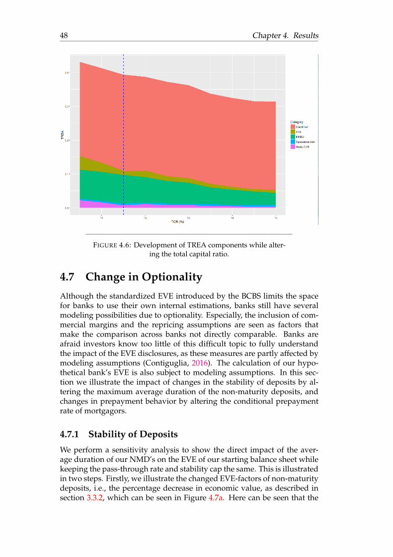
48 Chapter 4. Results
FIGURE 4.6: Development of TREA components while alter-ing the total capital ratio.
4.7 Change in Optionality
Although the standardized EVE introduced by the BCBS limits the spacefor banks to use their own internal estimations, banks still have severalmodeling possibilities due to optionality. Especially, the inclusion of com-mercial margins and the repricing assumptions are seen as factors thatmake the comparison across banks not directly comparable. Banks areafraid investors know too little of this difficult topic to fully understandthe impact of the EVE disclosures, as these measures are partly affected bymodeling assumptions (Contiguglia, 2016). The calculation of our hypo-thetical bank’s EVE is also subject to modeling assumptions. In this sec-tion we illustrate the impact of changes in the stability of deposits by al-tering the maximum average duration of the non-maturity deposits, andchanges in prepayment behavior by altering the conditional prepaymentrate of mortgagors.
4.7.1 Stability of Deposits
We perform a sensitivity analysis to show the direct impact of the aver-age duration of our NMD’s on the EVE of our starting balance sheet whilekeeping the pass-through rate and stability cap the same. This is illustratedin two steps. Firstly, we illustrate the changed EVE-factors of non-maturitydeposits, i.e., the percentage decrease in economic value, as described insection 3.3.2, which can be seen in Figure 4.7a. Here can be seen that the

4.7. Change in Optionality 49
(A) ∆EVE factors (B) ∆EVE
FIGURE 4.7: Impact of a change in the average duration ofcore NMDs on the EVE.
change in economic value is bigger when the average duration of core de-posits is longer. Subsequently, we use these factors as new input in order tovisualize the impact on balance sheet level for all six shocks to determinethe impact on the disclosed EVE.
Figure 4.7b illustrates the EVE values for a constant balance sheet underdifferent NMD repricing assumptions. Our hypothetical bank is fundedby 28.20 percent non maturity deposits, which is low compared to the49.50 percent overnight deposits to total EU household savings (Euro AreaStatistics). Despite this, the EVE is affected heavily by a change in dura-tion, in particular for the parallel shocks. A low duration of core deposits,i.e., less stable deposits, increases the magnitude of the alternative interestscenarios on balance sheet level, as deposits reprice earlier, which increasesthe gap between the repricing maturities of assets and liabilities. We fur-thermore observe that for an average duration of core deposits of two yearsand less, deposits are found not efficient compared to other short-termfunding sources, as our model decreased its position instead of allocatingnew business. At this point, the benefits of the deposits, i.e., the low in-terest expenses, do not weight the disadvantages, i.e., the instability in theform of a high stressed cash-outflow factor and relatively low duration.Moreover, more stable funding with a higher duration against the sameinterest expense is possible in the form of covered bonds.
4.7.2 Prepayment Behavior of Mortgagors
The second source of optionality we analyze is the conditional prepaymentrate. Given an optimal value-minimizing call policy, a mortgage shouldnever be paid off early when the refinancing cost exceeds the coupon value.Similarly, a mortgage should be paid off early if the current coupon exceedsits refinancing costs. However, in both cases we see mortgagors not alwaysact rationally, as in the former scenario prepayments still occur and in thelatter scenario the maximum amount of prepayments are not made (Dunnand McConnell, 1981). In the current standardized EVE measure, the pre-payment rates are stressed by 20 percent to reflect the change in prepay-ment behavior. We illustrate the sensitivity of change in prepayment rates

50 Chapter 4. Results
(A) CPR stress factor
(B) CPR
FIGURE 4.8: Impact of a change in the prepayment behavioron the EVE.
in two manners. Firstly, we stress the magnitude of the change in prepay-ment rates by increasing the stress factors of the CPR, which will result inhigher differences in duration of mortgages across alternative interest ratescenarios. Lastly, we illustrate what a change in expected base CPR willcause in terms of EVE.
Figure 4.8a illustrates that by increasing the stress factor for interestrate scenarios, the magnitude of the EVE increases. The parallel shocks areaffected the most followed by the steepener and flattener scenarios. Anincrease in rationality regarding the optimal value-minimizing call policy

4.8. Conclusions 51
described above would result in an increasing difference in cash flow un-der the interest rate scenarios compared to the base case. This will, as Fig-ure 4.8a shows, result in higher economic capital losses or less economiccapital gains under alternative interest rate scenarios.
Besides, a change in expected prepayment behavior in the base casecan also result in different values for the EVE. Although prepayment ratesare based on multiple years of payment data, a change in the conditionalprepayment rate can cause an offset in the EVE values on the longer term.Figure 4.8b indicates that given a constant balance sheet, an increase inprepayment rates of one percent causes an increase in EVE of 8.88 percentfor the parallel down scenario due to premature cash flows. Likewise, adecrease in prepayment rates of one percent causes an increase of 5.48 per-cent for the parallel up scenario due to a longer duration. The third andfourth scenario are less affected. Finally, the shocks in the short rates arehardly affected, due to the fact that these scenarios do not shock the yieldcurve for longer maturities.
4.8 Conclusions
This chapter answers the remaining sub-questions:
• How severely does a bank’s interest rate risk appetite affect its earnings?
We previously defined the interest rate risk appetite by a combination ofboth the EVE and NII. We illustrated the effect of setting our stylized bank’sinterest rate appetite using different limits on the EVE and NII. We ob-served that the EVE limits term transformation over all assets and liabili-ties, and with this, has the biggest impact on the interest rate spread. In-creasing the EVE from a conservative 4% to the maximum threshold of15% increased the return on equity with 1.12%. The NII could be hedgedrelatively cheaply by our model using one year swap contracts and haslittle impact on the interest rate spread. However, the observed two yearNII was, even though the one year NII and EVE were within boundaries,still substantial, which could result in high rollover costs of hedging instru-ments.
• What is the impact of stricter capital requirements on the potential interestrate spread and the impact of changes in key modeling assumptions on theinterest rate risk exposure of a bank?
We included the weighted interest rate risk exposure in the total risk ex-posure amount. Here, the total capital ratio is used as a scalar for capitalrequirements. We observed that the interest rate risk taking is more af-fected by an increase in capital requirement than other TREA components.This indicates that, given the capital indicator of 12.5 times the EVE used,the return per allocated capital is higher for credit risk exposure.

52 Chapter 4. Results
Furthermore, the sensitivity analysis concluded that our bank’s interestrate risk exposure is highly affected by changes in the model parametersreflecting the optionality embedded in banking products. This indicatesoption risk is something banks should monitor properly, as a bank’s inter-est rate risk exposure over time could be affected by changes in the stabilityof non-maturity deposits and client prepayment behavior. An opportunis-tic estimation of these parameters could therefore result in a severe under-estimation of a bank’s interest rate risk exposure.

53
Chapter 5
Conclusion, Discussion andFurther Research
The current low interest environment combined with increasing compe-tition results in more risk taking by banks in order to still make decentearnings (Memmel, 2011). The BCBS introduced new guidelines on howto manage interest rate risk to promote a resilient and balanced interestrate risk appetite. We used these guidelines complemented by other reg-ulatory requirements to see the impact of interest rate risk measures on abank’s risk taking, behavior and return on equity and with this, addresseda method for improving a bank’s balance sheet.
Firstly, we discuss our findings and address the answer to our mainquestion: What would be the impact of stricter regulation on interest rate risk inthe banking book and how could a bank improve its balance sheet given its interestrate risk appetite?. Furthermore, we discuss the limitations and possibilitiesfor further research.
5.1 Conclusions
We illustrated the effect of including non-parallel shifts in the yield curvein the EVE calculation. Although the required capital for interest rate riskis not affected solely by parallel shocks yield curves, banks are obliged todisclose parallel shocks of 200bps to the public to promote greater trans-parency and comparability. We observed that disclosing values of paral-lel shocks does not reflect the interest risk taking of a bank properly, asour bank could expose itself heavily to non-parallel shocks. As a result,the objective in form of the return on equity was not affected much byfurther restricting exposures to parallel shocks only. However, includingnon-parallel shocks in the simulation resulted in a decrease in exposure tonon-parallel scenarios for our hypothetical bank by matching the repricingmaturities more properly. As a result, the return on equity also decreasedby roughly 1.1 percent for conservative IRRBB limits (EVE of four percent)and 0.5 percent for a more risky IRRBB appetite (EVE of 15 percent) com-pared to restricting only parallel shocks.
Going forward, we showed that a balance sheet allocation consideringonly long-term measures while optimizing the short-term returns could

54 Chapter 5. Conclusion, Discussion and Further Research
result in a high earnings volatility on the short-term of as much as six per-cent. On the other hand, by focusing solely on a one year change in netinterest income, our hypothetical bank will expose itself to the maximumEVE threshold in its search for yield as would be expected. Following fromthis, the two year difference in net interest income following from interestrate shocks can also be significant, which can result in high rollover cost ofhedging instruments in order to keep the one year NII at the desired level.
Banks are obliged to hold capital for interest rate risk according to theinternal capital adequacy assessment process (ICAAP). To complete ourmodel, we used the proposed standardized method of the BCBS to com-pute the risk weighted exposure amount for interest rate risk as an ap-proximation for the required capital for interest rate risk. We implementedthis charge by including this weighted exposure as a building block of abank’s total risk exposure amount. By doing so, we included capital forinterest rate risk in the banking book in the total capital ratio. What weobserved during the simulation, is that the amount of required capital forinterest rate risk has a negative correlation with interest rate risk takingof our bank as would be expected. We also observed that the regulatorythresholds on the EVE are not sought while improving the spread in caseIRRBB risk taking is included in the capital allocation in the form of 12.5times the EVE. Instead, our hypothetical bank searches for an optimum be-tween the allocation of capital over credit risk and interest rate risk to max-imize the interest rate spread. This optimum is found at an EVE of eightpercent for a total capital ratio of 12 percent. Subsequently, the weightedinterest rate risk exposure amount decreased more during tighter capitalstandards compared to the weighted credit risk exposure amount. Ourfindings indicate that, by using the EVE measure as capital indicator, in-terest rate risk taking is more sensitive to tighter capital requirements thancredit risk taking. The reasons for that are a lower return in relation tothe required capital and the possibility to decrease its exposure throughinterest rate swaps.
In Basel’s latest guidelines on interest rate risk in the banking book wealready observed more flexible caps on the amount of core deposits, themaximum average duration of non-maturity deposits and the magnitudeof the prepayment rate shocks compared to the draft version of 2015. Thisleaves more space for banks to fill in these parameters according to their in-ternal measurements, which supports limiting the gap between standard-ized measures and outcomes resulting from internal models. Our findingsunderline this decision space for banks to fill in these parameters accordingto their best estimation, as our findings show that a bank’s EVE is highlydependent on model assumptions regarding both the sources of optional-ity included in our model. We also conclude that a change in optionality isa risk banks should consider with great care, as we showed that changes inoptionality embedded in banking products and deposits can cause signif-icant changes in future EVE values. An opportunistic estimation of theseparameters could therefore result in a severe underestimation of a bank’sinterest rate risk exposure.

5.2. Discussion and Further Research 55
In summary, our main three conclusions towards answering our re-search question are:
1. As implied by the BCBS, a combination of limits on both NII andEVE is necessary in order to install a prudent interest rate risk man-agement. While maximizing the return on equity, a bank will exposeitself to the maximum EVE-threshold, likely under multiple alterna-tive interest rate scenarios, in order to maximize the yield from termtransformation. The NII measure has little impact on the interest ratespread, but is of essence in order to limit earnings volatility. How-ever, the one year NII combined with relatively loose limits on theEVE might not be sufficient, as we laid out that the resulting twoyear NII could result in high rollover costs of hedging instruments.
2. Including a direct capital requirement for a bank’s interest rate expo-sure in the form of 12.5 times the standardized EVE measure has adegrading effect on interest rate risk taking, as the return on requiredcapital is higher for credit risk compared to interest rate risk this way.
3. A bank’s interest rate risk exposure is highly sensitive to assump-tions in optionality. Even small changes in clients’ rationality regard-ing prepayment, i.e., a change in the prepayment multiplier underalternative scenarios, and in repricing characteristics of non-maturitydeposits could result in a significant change in a bank’s interest raterisk exposure.
Using the proposed model, a bank can get insights in a more profitablebalance sheet allocation giving restrictions on prudential measures, visu-alize the impact of interest rate risk limits on its potential expected return,as well as determine the impact of possible changes in client behavior asresult of behavioral optionality embedded in banking products.
5.2 Discussion and Further Research
With our thesis we proposed a method to incorporate interest rate riskmeasures in balance sheet improvement using a point in time optimiza-tion given a set of assets and decision space. By using this model, we illus-trated the impact of more severe interest rate regulations in terms of NIIand EVE exposure and capital requirements while improving a bank’s re-turn on equity. However, creating a complete representation of the realityis nearly impossible. For the balance sheet input, we were bounded by theavailable balance sheet data, hence we were forced to make assumptionson distributions of assets’ and liabilities’ cash flows and fixed interest rateperiods. We covered this by using available performance reports of DutchRMBSs, annual reports and assumed the uniform distribution for allocat-ing assets of repricing maturities where needed. Furthermore, due to alack of data about realistic interest rate swap portfolios, we used the cur-rent swap rates to hedge our starting exposure, using a set of ten swaps.

56 Chapter 5. Conclusion, Discussion and Further Research
As interest rates are currently lower than ten years ago, the swap expensestend to be less compared to real swap expenses of a bank. Subsequently,interest rate swaps are traded over the counter and can be customized toa bank’s need. By assuming a set of only ten interest rate swaps, only thenotional amounts between swap maturities can be determined. In orderto make it more representative, interest rate swap exposures could be in-cluded in more detail. Moreover, we assumed our bank can influence itsnew acquired mortgages with a high level of precision. In real life, banksare less able to determine this acquisition. However, a bank is able to hedgeits interest rate exposure more precisely to match repricing dates using cus-tomized notional amounts. This partly compensates for the discussed in-efficiency, as swap rates resemble the change in interest fixed period formortgages.
Our model indicates an optimal distribution of capital given a maxi-mum level of risk exposure. Yet, it does not advise on the level of capital,nor we included other forms of capital than Tier 1 capital. Moreover, wedo not include transaction costs, which a bank does pay in switching posi-tions.
We included the main sources of embedded optionality in our model.Other forms of optionality, for instance embedded options to extend theduration or change interest rate characteristics, are not covered, but cancause a change in cash flows and interest rate fixed periods under interestrate scenarios.

57
Appendix A
Interest Rate Scenarios
In our model, we quantify the interest exposure of our hypothetical bankby determining the impact of interest rate shocks on its economic valueand earnings. We use six prescribed shocks who cover all possible yieldcurve movements. More on the calculation of these shocks can be found inBCBS (2016).
The first scenario we use is a parallel shift upwards. For all maturities,so for every time bucket, the yield curve increases with the same amount.The conditional prepayment rate of fixed loans decreases with 20 percent,while the term deposit redemption rate increases with this same numberfor this stress scenario. The same is the case for the second scenario, whereinterest rates for every time bucket decreases with a prescribed number.The decrease of interest rates results in a higher conditional prepaymentrate of fixed loans (+20 percent) and a lower term deposit redemption rate(-20 percent).
Expectations of investors about future interest rates can alter the steep-ness of the yield curve. Under the third scenario, interest rates are alteredto create a steepener yield curve: interest rates for shorter maturities willbe decreased and longer maturity rates will be increased. Subsequently,this scenario comes includes a decrease in the amount of prepayments onfixed loans and with a lower term deposit redemption rate. For the fourthscenario, a flattener yield curve, the effect the other way around.
The fifth and sixth scenario cover the changes in the short rate. Thesame effect on prepayments and deposit redemption rates as the parallelshocks are applicable for these scenarios. A summary of the scenarios andmultipliers can be seen in Table A.1. The final shocks to the maturity buck-ets can be seen in Figure A.1. The base and alternative interest rate curvesare illustrated in Figure A.2.
TABLE A.1: Interest rate shock-scenarios and multipliers.
Number (i) Scenario CPR multiplier TDRR multiplier1 Parallel up 0.8 1.22 Parallel down 1.2 0.83 Steepener 0.8 1.24 Flattener 1.2 0.85 Short rate up 0.8 1.26 Short rate down 1.2 0.8

58 Appendix A. Interest Rate Scenarios
FIGURE A.1: Euro interest rate shock scenarios set out by theBasel Committee on Banking Supervision.
FIGURE A.2: Base and alternative interest rate scenarios.

59
Appendix B
Distribution of non-maturitydeposits
Definition B.1. Non-maturity deposits are liability instruments for whichthere are two embedded options: one held by the bank (the right to changethe interest rate) and a second held by the depositor (the right to withdrawits funds).
Due to the behavioral factor, NMDs can cause uncertainty and withthis, potential future interest rate exposure. Furthermore, behavioral riskis heterogeneous, as factors rely on several parameters, such as the age ofcustomers and geographic location. An example of heterogeneous option-ality is the conditional prepayment rate (CPR), which we included in ourmodel. In the Netherlands, clients are allowed to pay an additional 10% oftheir mortgage annually without receiving a penalty for it. In other coun-tries, often other contractual terms are set regarding prepayment.
Banks use behavioral models to forecast the extend of withdrawals ofdepositors, but outcomes across banks can be very different, which makescomparing interest rate risk exposure across banks hard. Regulators ac-knowledge the heterogeneity, but restrict the average duration, as it cancause an underestimation of interest rate risk. In the consultation paper onIRRBB (BCBS, 2015), the BCBS proposed a more strict treatment of NMDs,with a maximum repricing date of 5 years versus an average of 4.5 and5 years in the final guidelines (BCBS, 2016). For our model we use twotypes of non-maturity deposits: demand deposits and savings deposits.For these NMDs, we combine the treatment for NMDs proposed in theconsultation paper with the restrictions of the final guidelines by usingthe Time Series Approach (TSA). For this, we distribute the NMDs overtransactional and non-transactional deposits. The Stability cap and Pass-through floor can be seen in Figure B.1. We determine the stable amountof these deposits and determine the amount of core deposits, given by thestability cap:
Amount of core deposits = N · S · (1− P ) (B.1)
Where:
N = the total amount of depositsS = the stability capP = the pass-through floor

60 Appendix B. Distribution of non-maturity deposits
FIGURE B.1: Subclasses of non-maturity deposits.
TABLE B.1: Stability caps and pass-through floors for NMDs.
Stability cap (%) Pass-through floor (%) Implied cap (%)Demand deposits 80 25 60 (=0.8 ·(1-0.25))Savings deposits 70 30 49
All core deposits are uniformly distributed such that the average repric-ing time equals the maximum average repricing time described in the fi-nal guidelines. Non-core deposits are seen as not stable, and are thereforeslotted in the overnight bucket. The final distribution is illustrated in Fig-ure B.2.

Appendix B. Distribution of non-maturity deposits 61
FIGURE B.2: Distributions of demand deposits and savingsdeposits over buckets.


63
Appendix C
Interest rate swaps
Despite that the fair value of the interest rate swaps at starting point inthe simulation equals zero, interest rate swaps do have an impact on riskmeasures. In this section, we will elaborate on the impact of interest rateswaps on the ∆EVE, ∆NII and the additional capital requirements as aresult of counterparty credit risk and credit value adjustment.
C.1 Impact On Economic Value And Net InterestIncome
For our model we use four interest rate swaps with different maturities.To include the swaps without placing them on the balance sheet, we deter-mine the par coupon, such that the fair value of the swaps equal zero.
TABLE C.1: Par rates interest rate swap (source: Bloomberg).
Time to maturity Par coupon1 year -0.28508%2 year -0.23082%3 year -0.15883%4 year -0.07302%5 year 0.03263%10 year 0.65343%12.5 year 0.88955%15 year 1.06439%17.5 year 1.16122%20 year 1.24902%
C.2 Counterparty Credit Risk
The counterparty credit risk is calculated using the standardized coun-terparty credit risk approach (BCBS, 2014b). This calculation consist oftwo components: a risk weight and the exposure amount, where the ex-posure amount is the sum of the replacement cost (RC) and the potential

64 Appendix C. Interest rate swaps
future earnings (PFE) multiplied by a factor alpha, which equals 1.4, writ-ten mathematically:
Exposure at default under SA = EAD = alpha · (RC + PFE ) (C.1)
Since we use fixed par rates, resulting in a fair value of the interest rate ofzero, the replacement cost are zero. The potential future exposure can becalculated using the formula:
PFE = SF IR · |δi · dIRi ·MF typei | (C.2)
Where:
SF = supervisory factor, for interest rate swaps equal to 0.5%.δi = supervisory delta.dIRi = adjusted notional.MF type
i = maturity factor, which is 1 for maturities higher than one year.
dIRi = TradeNotional · exp(−0.05 · Si)− exp(−0.05 · Ei)
0.05(C.3)
Where:
Si = begin date of swap iEi = end date of swap i
The potential future exposure is multiplied by the risk weight of thecounterparty, in our case a bank, to determine the counterparty credit riskexposure.
C.3 Credit Valuation Adjustment
The CVA capital charge is calculated using the standard approach describedin article 384 of the CRR (BCBS, 2014b). Based on this method, the capitalcharge is calculated as the sum of all CVA capital charges calculated oncounterparty level. For simplicity we assume that all interest rate swapsare with one counterparty. The CVA capital charge can be calculated usingthe following formula:
K = 2.33·√h·
√(∑i
0.5 · wi · (Mi · EADtotali −M
hedgei · Bi −
∑ind
wind ·Mind · Bind)2 +
∑i
0.75 · w2i · (Mi · EADtotal
i )−Mhedgei · Bi)2
(C.4)
As we do not include CVA hedges, the calculation can be simplified to:
K = 2.33·√h·
√√√√(∑i
0.5 · wi ·Mi · EAD totali
)2
+∑i
0.75 · w2i ·(Mi · EAD total
i
)2
(C.5)Where:

C.3. Credit Valuation Adjustment 65
h = the one-year risk horizon in units of a year "1"wi = the counterparty weight of iEAD total
i = the exposure at default of counterparty iMi = the effective maturity of the transactions with counterparty i


67
Appendix D
Risk Measures
D.1 Capital Requirements
D.1.1 Total Capital Ratio
The minimum amount of capital is determined through the calculation ofthe Total Risk Exposure Amount (TREA). According to the minimum cap-ital requirement, the capital divided by the sum of risk exposure of a bank(i.e. interest rate risk exposure excluded) should be higher than 10.5% (Eu-ropean Parliament and the Council of the European Union, 2013).
TCR =y6
TREA≥ 10.5% (D.1)
We define the following building blocks of the TREA of our bank:
• Credit risk exposure. We calculate this exposure using the standard-ized approach in which assets get a defined risk weight. For theweighting scheme of assets we refer to Table E.2.
• Operational Risk Exposure, which is calculated by taking 15 percentof the annual gross income.
• Exposure as a result of derivative exposure, for which we refer toAppendix C.
In a later scenario, we include an approximation for interest rate risk byadding the interest rate exposure to our bank’s TREA in order to determinethe minimum capital requirement on interest rate risk in the banking book:
• Interest rate risk exposure, 12.5 (i.e. the inverse of the minimum 8%risk-based capital requirement) times the EVE-measure.
The TCR of the proxy banks used for constructing our stylized balancesheet variates between 15.5 and 19.3 percent. A note should be made thatthese values only include exposures captured in pillar 1 and so do not re-flect all risks, hence the relatively big difference compared to the regulatoryminimum.
68 Appendix D. Risk Measures
D.1.2 Leverage Ratio
One of the causes cause of the global financial crisis was the build-up ofexcessive on- and off-balance sheet leverage in the banking system. Inmany cases, banks built up excessive leverage while apparently maintain-ing strong risk-based capital ratios. Therefor, the BCBS finds the leverageratio (Formula D.2) a necessary supplementary measure to the risk-basedcapital measures. More on the leverage ratio can be found in Basel III lever-age ratio framework and disclosure requirements (BCBS, 2004a).
Leverage ratio =Capital measure
Exposure measure≥ 3% (D.2)
D.2 Liquidity
The first known literature on liquidity risk dates from 1876, when Knies(1976) stressed the need for cash buffers to compensate for possible gapsbetween cash in and out flows of banks in case the precise maturity couldnot be controlled.
Liquidity risk encompasses the risk a bank may be unable to meet shortterm financial demands and results from size and maturity mismatches ofassets and liabilities (Bessis, 2011). A bank with long-term commitmentsand short-term funding generates cash-flow deficits. The liquidity risk re-sults from insufficient resources to fund the long term assets, as a resultof a decrease in available funds. Liquid assets, such as cash and govern-ment bonds, protect banks from market tension, as they can be used asalternative source of funding for short term obligations. The cost of liq-uidity for banks often refers to the cost of maintaining liquidity ratios at aan adequate level, i.e. generate more stable long-term funding or holdingsufficient HQLA.
Since the global financial crisis of 2008, the focus of the BCBS on liquid-ity risk has increased. Despite their adequate capital levels, many banksexperienced difficulties during the early "liquidity phase" of the financialcrisis in 2007 as a result of not managing liquidity risk in the right man-ner. Before the crisis, the asset markets were resilient and funding could beacquired against low costs. A rapid reversal in market conditions showedthe volatility of liquidity, resulting in severe stress scenarios under banks.According to Ferrari and Ruozi (2009), the insufficient liquidity of banks’is rather the result of the financial crisis than the cause of it. Instead, theseauthors state the crisis comes forth from the lack of proper principles of ahealthy and prudent management together with pursuing too much short-term profits.
To promote both the short- and long-term resilience of banks’ liquidityrisk profiles and in order to manage and monitor liquidity risk, the BCBSintroduced two liquidity measures (BCBS (2013a), BCBS (2014a)): the liq-uidity coverage ratio (LCR) and the net stable funding ratio (NSFR). The

D.2. Liquidity 69
LCR is developed to ensure that banks have an adequate stock of unen-cumbered high-quality liquid assets (HQLA). Here, the adequate amountof HQLA is quantified as the difference in cash-flows for a 30 day liquid-ity stress scenario. The NSFR requires banks to maintain a stable fundingprofile in relation to their balance sheet activities. By maintaining a stablefunding profile, the likelihood that disruptions to a bank’s regular sourcesof funding will erode its liquidity position in a way that could increase therisk of its failure will be reduced.
D.2.1 Liquidity Coverage Ratio
The liquidity Coverage Ratio (LCR) promotes short-term resilience by pre-scribing the sufficient level of high-quality liquid assets (HQLA). The amountof HQLA is quantified by a 30-day liquidity stress period. HQLA are char-acterized by their low risk, ease and certainty of valuation, absence ofwrong-way risk and are traded on developed and recognized exchanges,and so can easily be liquidated (BCBS, 2013a). The BCBS assigned HQLA-factors to the asset classes based on this marketability.
LCR =Stock of HQLA
Total net cash outflows over the next 30 calender days≥ 100%
(D.3)
D.2.2 Net Stable Funding Ratio
The net stable funding ratio (NSFR) requires banks to maintain a stablefunding profile proportional to its balance sheet activities in order to re-duce the likelihood that disruptions to a bank’s regular sources of fundingwill erode its liquidity position in a way that could increase the risk of itsfailure and potentially lead to broader systemic stress.
NSFR =Available amount of stable fundingRequired amount of stable funding
≥ 100% (D.4)


71
Appendix E
Balance Sheet Definition
E.1 Asset Definitions
Cash and Balances with Central BanksCash and balances with Central banks are assumed to reprice overnightand are mainly held as a liquidity buffer.
Loans and Advances to banksLoans and advances to banks with subclass maturity and are distributedfocused on short term repricing.
Government BondsBonds issues by sovereigns. Subclass: Credit rating and Maturity.
Retail MortgagesThis asset class includes loans secured by residential property and can bedivided in subclasses based on loan-to-value and maturity.
Other AssetsThis asset class encompasses other non-interest bearing assets and is there-for excluded from interest rate risk calculations.
Interest Rate SwapsFinancial agreement between two parties to exchange a series of interestpayments without exchanging the underlying debt. Subclass: maturity.
E.2 Liability and Equity Definitions
Due to BanksDeposits from banks. Subclass: maturity.
Demand DepositsFunds held in an account from which deposited funds can be withdrawnat any time without any advance notice to the depository institution. Sub-class: maturity.

72 Appendix E. Balance Sheet Definition
Savings DepositsInterest-bearing deposits that provides a modest interest rate. Sub-class:maturity.
Term DepositsDeposits that has a fixed term. Subclass: maturity.
Secured FundingSecured funds, on the shorter term (<1Y) commercial paper, on the longerterm bonds.
Other LiabilitiesThis asset class encompasses other non-interest bearing liabilities and istherefor excluded from interest rate risk calculations.
EquityBanks’ shareholders’ equity. This class is held stable over the simulationand is excluded from interest rate calculations by regulation.
E.3 Balance sheet input

E.3.Balance
sheetinput73
TABLE E.1: Balance sheet distribution and data sources.
Distribution Current return New return SourceAssetsCash and equivalents O/N ECB deposit rate ECB deposit rate Bloomberg
Mortgages According tomortgage portfolio
According tomortgage portfolio Current market rates
Dolphyn (2016),Goldfish (2016),hypotheekrente.nl
Government bond (AA-) Uniform <10Y 5Y average Current yields BloombergGovernment bond (A- to A+) Uniform <10Y 4Y average Current yields BloombergLoans and advances to banks Uniform <1Y 1Y average Swap rate + CDS spread BloombergLiabilitesDue to banks Uniform <1Y 1Y average Swap rate + CDS spread BloombergDemand deposits TIA 0% 0% -Savings deposits TIA Average market rates Average market rates Spaarrente.nl
Term deposits Uniform, in line withAnnual Reports Average market rates Average market rates Spaarrente.nl
Secured funding Uniform <7Y 5Y average CB yield ING covered bond yield Bloomberg

74A
ppendixE.
BalanceSheetD
efinition
TABLE E.2: Asset starting exposure and risk factors.
Asset Start RW <1Y RW >1Y HQLA CI-Factor RSF <6M RSF 6M-1Y RSF ≥1YCash and equivalents 1.0% 0% 0% 100% 0 0%NHG 25,8% 5% 5% 0% 0,7% 50% 50% 65%Loan-to-value <60% 22,8% 30% 30% 0% 0,7% 50% 50% 65%Loan-to-value <80% 18,0% 35% 35% 0% 0,7% 50% 50% 65%Loan-to-value <102% 17,3% 55% 55% 0% 0,7% 50% 50% 65%Government bonds (AA-) 1,0% 0% 0% 100% 0% 5% 5% 5%Government bonds (A- to A+) 1,4% 20% 20% 85% 0% 15% 15% 15%
Loans and advances to banks 7,7% 20% 50% 0% According tomaturity 0 50% 50%
Other assets 4,9% 60% 60% 35% 0% 100%
TABLE E.3: Liability starting exposure and risk factors.
Starting Weights Cash Outflow Factor ASF Factor <6M ASF Factor 6M-1Y ASF Factor ≥1YDue to banks 0,7% 100% 0 50% 50%Demand deposits 12.0% 5%, 10% 90% 90% 100%Savings deposits 16,2% 5%, 10% 95% 95% 100%Term deposits 15,9% 100% 95% 95% 100%Secured funding 45,6% 100% 0 50% 100%Other liabilities 5,2% 0% 50%Equity 4,5% 0% 100% 100% 100%

E.3. Balance sheet input 75
FIGURE E.1: Starting distribution of stylized balance sheet
FIGURE E.2: Interest income and expense of current portfolio

76 Appendix E. Balance Sheet Definition
FIGURE E.3: Interest income and expense of new business
FIGURE E.4: Proposed changes in balance sheet allocation

77
Appendix F
Interest Rate Disclosures
The (BCBS, 2016) introduced a more standardized method to systemati-cally quantify the interest rate exposure of banks in order to promote trans-parency and comparison across banks. The price that has to be paid forstandardization is the possibility of misrepresenting the reality. Becauseof this, banks still have certain freedoms, such as determining the repric-ing distribution of NMDs. In order to compare the outcomes of the dis-closed values across banks, banks need to disclose high-level assumptionson model choices.The new guidelines on interest rate risk in the banking book of the BCBSinclude new public disclosure requirements. Banks are required to disclosethe EVE impact under six prescribed interest rate scenarios. Furthermore,information on the maximum and average duration of deposits and as-sumptions that have been made regarding repricing of NMDs should alsobe disclosed to both the regulator and the public. In general, banks areafraid investors have too little knowledge of this difficult topic to fully un-derstand the disclosures. Furthermore, banks fear that the disclosures willcontain sensitive information (Contiguglia (2016), BBA (2015)). As a result,banks expect that too much attention will be focused on the disclosed EVEoutcomes, ignoring the bank’s interest rate risk management.Besides, disclosure of quantitative parameters, such as current NMD repric-ing assumptions, can be used by competitors to calibrate their models(BBA, 2015). Banks usually base the interest on savings accounts by bench-marking their rates with the expected rates of their competitors. If informa-tion about repricing assumptions is publicly available, it gives competitorsa better idea of the prices a bank will offer and anticipate on this.The disclosing requirements could also give competitors insight into indi-vidual banks’ pricing and hedging strategy. Banks claim that disclosingall fixed prescribed scenarios would effectively be the same as disclosingthe duration of any bank’s portfolio. This could lead to market partici-pants frontrunning a bank’s hedging needs based on its portfolio charac-teristics (Wilkes, 2016). Another argument against disclosing the interestrate shocks is that investors will misinterpret the disclosed EVE values,and will see the disclosed EVE values as a going concern measure. There-fore, banks will appear to be at greater risk due to the absence of mitigationstrategies, which will cause unnecessary panic in the market (BBA, 2015).Finally, the EVE is only standardized to some extent, which can cause moreconfusion under investors. For instance, a bank has the choice to include

78 Appendix F. Interest Rate Disclosures
or exclude commercial margins. In case the bank chooses to include them,commercial margins should be included in the discount rate, which canresult into different outcomes. Also the treatment of NMDs is not entirelystandardized. There are caps on the amount of core deposits and averageduration, but distributions and durations can still differ across banks.

79
Bibliography
Achmea Bank (2015). Achmea Bank, 2015 Annual report.Aegon Bank (2015). Aegon Bank, 2015 Annual report.ASR Bank (2015). ASR Bank, 2015 Annual report.Baldan, C. and F. Zen (2013). How have banks adjusted to higher capital require-
ments?Bank for International Settlements (2015). Abouth the Bank for International
Settlements. https://www.bis.org/about/history.htm. Ac-cessed: 02-01-2017.
BBA (2015). A response to the Basel Committee’s consultative document on In-terest rate Risk in the Banking Book.
BCBS (1993). Measurement of Banks’ Exposure to Interest Rate Risk.— (1997). Principles for managing interest rate risk.— (2004a). Basel III leverage ratio framework and disclosure requirements.— (2004b). Principles for the management and supervision of interest rate risk.— (2006). International Convergence of Capital Measurement and Capital Stan-
dards.— (2010). Basel III: A global regulatory framework for more resilient banks and
banking systems.— (2013a). Basel III: The Liquidity Coverage Ratio and liquidity risk monitoring
tools.— (2013b). Fundamental review of the trading book: A revised market risk frame-
work.— (2014a). Basel III: the net stable funding ratio.— (2014b). The standardised approach for measuring counterparty credit risk
exposures.— (2015). Consultative Document on interest rate in the banking book.— (2016). Standards for Interest rate risk in the banking book.Bessis, J. (2011). Risk management in banking. John Wiley & Sons.Bhattacharya, S. and A. V. Thakor (1993). “Contemporary banking theory.”
In: Journal of financial Intermediation 3, pp. 2–50.Bucksler, J. and A. H. Chen (1986). “An economic analysis of interest rate
swaps”. In: The Journal of Finance 41, pp. 645–655.Chen, C. and A. Chan (1989). “Interest rate sensitivity, asymmetry and
stock returns of financial institutions”. In: Financial Review 24.3, pp. 457–473.
Cohen, B. H. (2012). Liquidity risk and interest rate risk on banks: are they re-lated?
Contiguglia, C. (2016). EBA stress test shines light on interest income hedgingdilemma. www.risk.net. Accessed: 28-01-2017.

80 BIBLIOGRAPHY
Cox, J. C., Jr. J. E. Ingersoll, and S. A. Ross (1985). “A theory of the termstructure of interest rates.” In: Econometrica: Journal of the EconometricSociety 69, pp. 385–407.
De Nederlandsche Bank N.V. (2005). Guidelines on interest rate risk in thebanking book.
Delta Lloyd Bank (2015). Delta Lloyd Bank, 2015 Annual report.Dolphin Master Issuer B.V. (2016). Dolphin Monthly Portfolio and Performance
Report.Drehmann, M., S. Sorensen, and M. Stringa (2006). “Integrating credit and
interest rate risk: A theoretical framework and an application to banks’balance sheets. In Bank for International Settlements Conference on“Risk management and regulation in banking”. In: Basel 6, pp. 1–33.
Dunn, K. B. and J. McConnell (1981). “Valuation of GNMA Mortgage-BackedSecurities.” In: The Journal of Finance 36, pp. 599–616.
EBA (2015). Guidelines on the management of interest rate risk arising from non-trading activities.
English, W.B. (2002). “Interest rate risk and bank net interest margins”. In:BIS Quarterly Review 12.
European Parliament and the Council of the European Union (2013). Reg-ulation No 575/2013 of the European Parliament and of the Council.
EY (2016). Insights from EY European IRRBB Survey 2016 for banks.Ferrari, R. and R. Ruozi (2009). “Liquidity risk in banks: economic and reg-
ulatory aspects profiles (Translation)”. In: Banche e Banchieri 2, pp. 85–101.
Flannery, M. J. (1983). “Interest Rates and Bank Profitability: AdditionalEvidence: Note.” In: Journal of Money, Credit and Banking 15, pp. 355–362.
Fraser, D.R., J. Madura, and R.A. Wigand (2002). “Sources of bank interestrate risk”. In: The Financial Review 37, pp. 351–367.
Goldfish Master Issuer B.V. (2016). Goldfish Monthly Portfolio and Perfor-mance Report.
Hellwig, M. (1994). “Liquidity provision, banking, and the allocation ofinterest rate risk”. In: European Economic Review 38.7, pp. 1363–1389.
Hull, J. (2012). Risk Management and Financial Institutions. John Wiley &Sons.
Jones, D. (2000). “Emerging problems with the Basel Capital Accord: Reg-ulatory capital arbitrage and related issues.” In: Journal of Banking andFinance 24, pp. 35–58.
Koch and MacDonald (2014). Bank management. Nelson Education.Kraft, D. (1994). “Algorithm 733: Tompfortran modules for optimal control
calculations”. In: ACM Transactions on Mathematical Software 20, pp. 262–281.
Maes, K. (2005). “Interest Rate Risk in the Belgian Banking Sector”. In: Na-tional Bank of Belgium.
Markowitz, H. (1952). “Portfolio selection”. In: The Journal of Finance 7,pp. 77–91.

BIBLIOGRAPHY 81
Memmel, C. (2011). “Banks’ exposure to interest rate risk, their earningsfrom term transformation, and the dynamics of the term structure.” In:Journal of Banking & Finance 35.2, pp. 309–338.
Memmel, C., A. Seymen, and M. Teichert (2016). Banks’ interest rate risk andsearch for yield: A theoretical rationale and some empirical evidence.
Nomura (2016). How low can Japan lower its rates? http://www.zerohedge.com/news/2016-02-03/how-low-can-bank-japan-lower-rates-ask-gold. Accessed: 28-02-2017.
Rajan, R. G. (2005). “Has financial development made the world riskier?NBER Working Paper”. In: NBER Working Paper No. 11728.
Wilkes, S. (2016). Basel interest rate risk disclosures "problematic". www.risk.net. Accessed: 28-01-2017.