the impact of intelligent agents on electronic markets...
TRANSCRIPT

The Impact of Intelligent Agents on Electronic Markets:
Customization, Preference Revelation and Pricing.
Ravi Aron: Arun Sundararajanr and Sivakumar ~iswanathani
44 West 4th Street, K-MEC 9-79,
New York, NY 10012-1126
Ph: (212) 998 0833
Fax: (212) 995 4228
March 2000
*The Wharton School, University of Pennsylvania. ravzaronQwharton.z~penn.edu
+Stern School of Business, New York University. [email protected] $Stern School of Business, New York University. suzswana8stern.nyu.edu
Center for Digital Economy Research Stem School of Business IVorking Paper IS-00-01

The Impact of Intelligent Agents on Electronic Markets:
Custornization, Preference Revelation and Pricing.
Abstract
Apart from reducing buyer search costs, web-based commerce has also enabled the use of
intelligent agent technologies that reduce seller search costs by targeting buyers, customizing,
and pricing products in real-time. Our model of an electronic market with customizable prod-
ucts analyzes the pricing, profitability and welfare implications of these agent-based technologies
that price dynamically, based on product preference and demographic information revealed by
consumers. We find that in making the trade-off between better prices and better customiza-
tion, consumers invariably choose less-than-ideal products. Furthermore, this trade-off impacts
buyers on the higher end of the market more, and causes a transfer of consumer surplus to-
wards buyers with a lower willingness to pay. As buyers adjust their product choices in response
to better demand agent technologies, sellers may experience reduced revenues, since the gains
from better buyer information are countered by the lowering of the total value created from
the transactions. We study the strategic and welfare implications of these findings, and discuss
managerial and technology development guidelines.
1 Introduction and rnot ivat ion
It has been observed by several researchers that electronic markets have the potential to transform
retail commerce, by reducing buyer transaction costs (Bakos, 1991, Malone, Yates and Benjamin,
1991). A number of papers have been written about the general problem of search that buyers
encounter when they attempt to locate sellers, and the resulting store location and product dif-
ferentiation choices that sellers make1. The approaches of these papers have also been adapted to
settings involving electronic markets, most notably in Bakos (1997).
W i l e the lowering of buyers' search costs is a crucial determinant of profits and welfare from
electronic commerce, electronic markets are also causing another, equally profound change in com-
merce, by enabling and lowering the costs of a complementary form of search. Sellers in elect,ronic
markets now have an unprecedented ability to accurately search for, target and customize for their
individual buyers. A recent article about Web-based commerce in The Economist explains that this
'See, for instance, Stigler, 1962, Diamond, 1971, and Salop, 1979.
Center for Digital Economy Research Stem School of Business IVorking Paper IS-00-01

"....is a move away from mass marketing, which starts with a product and finds customers to buy
it, towards an information-led, one-to-one marketing, which may ultimately sell each individual a
customized product."
Certainly, targeted selling existed well before commerce on the Web became popular. Sellers
have sought to market directly to individual consumers for many years - in North America alone,
this industry was worth $163 billion in 1998, and was responsible for three-fifths of the country's
total spending on advertising. However, traditional direct marketing is imprecise, with typical suc-
cess rates for mail-shot campaigns in mature markets being no better than 2%. The low conversion
rates are largely because direct marketers have been forced to rely on imprecise consumer prefer-
ence profiles, built using a combination of census data, questionnaires, electoral-roll information
and credit-card data. Such information lacks the granularity and reliability required for precise and
economically viable targeting.
Commerce on the Web mitigates this inadequacy in consumer information. Recent developments
in Internet-related technologies have made it feasible for sellers to obtain near-perfect information
on individual customers, and to provide products and services tailored precisely to the consumer's
individual preferences, thus making the transition from product-led marketing to consumer-led
marketing a reality. Foremost amongst them is the deployment and use of zntellsgent agents (for
a description of some of these agents, see Maes, 1994). The existence of these agents radically
transforms the dynamics of the buyer-seller transaction, as it creates. in some sense, an exclusive
market for each buyer-seller pair. It also makes mass customization on a per-customer basis
feasible. It opens up the possibility of perfect, first-degree price discrimination. Furthermore, it
enables merchants to make intelligent associations across buyers.
While similar agents are also used to facilitate buyer search, we study the class of intelligent
agents known as demand agents. These agents estimate buyer preferences, valuations and product
tastes, by combining consumer purchase histories with individual and site demographics. They use
this information to price and recommend products to these customers. They also provide buyers
with product information, and could help sellers design new products and marketing strategies.
Many agents use collaborative filtering - a technique that uses mathematical algorithms to factor
preferences and compare an individual's preferences with the preferences of other users - to make
recommendations based on these comparisons (see, for instance, Balabanovic and Shoham 1997,
Kautz, Selman and Shah 1997, Stohr and Viswanathan, 1999). Net Perceptions, for instance, sells a
demand agent with consumer profiling capabilities that remembers the preferences of shoppers based
on their past purchases. It is used by several major content aggregators and e-tailers (including
Amazon.com, CDNow, Lycos and Bluefly) to facilitate personalized, dynamic, and customized
shopping experiences. The Economist noted recently that "the true strength of Amazon.com
lies in the wealth of information it now has about readers. Publishers would kill to have this
information."
Center for Digital Economy Research Stem School of Business IVorking Paper IS-00-01

Newer technologies have enabled more sophisticated methods of consumer targeting. Dou-
bleClick, a Web-based advertising company, uses customer profiles (built from a combination of
site demographics, customer databases and buyer click-stream patterns) to send targeted advertis-
ing offers to people in real time. Other agents, such as the one used by Alexa.com, Dash.com and
WiseWire, learn from and react to users' browsing patterns. Techniques are now being developed
to mine these patterns of customer interaction, and use them to make custornized price and product
offers to Internet buyers (Dhar and Sundararajan, 1999). According to George Colony of Forrester
Research, these 'killer clicks' will shape the Internet economy, and the balance of market power will
tip towards players that understand and harvest this new source of information.
The success of companies that were early adopters of agents like Firefly and Netperceptions sug-
gests huge potential gains for that the companies who lead the way in developing and adopting more
advanced demand agents. Certainly, dynamic pricing on the Internet is gaining increased attention
in corporations (Datta and Segev, 1999), and is also being demanded by consumers. As reported by
Business 2.0: "..according to a Jupiter survey in mid-1998, 80 percent of consumers expressed price
elasticity as one of their top considerations in on-line buying decisions. This fact, coupled with
the power of comparison shopping technologies such as Amazon.comls Junglee Canopy or Excite's
Jango, are compelling reasons for on-line merchants to invest in and develop rapid-response pricing
mechanisms." (Singh, 1999). In a recent report on agent-driven marketplaces, Wired Magazine
profiled Charles Plott of Caltech. who experiments with markets that can manipulate both prod-
ucts and price in real time. According to Plott, in agent-driven markets, "..what is being sold is
simultaneously being crafted with the price." There are numerous other markets being developed
at leading companies, such as Jeff Kephart's simulated system of intelligent agents, that can infer
buyer preferences and negotiate prices dynamically (Bayers, 2000). In their March 2000 Internet
market strategies report, The Yankee Group, an influential e-commerce research firm predicts that
most shopping agents ('bots') will soon incorporate dynamic pricing technology (Yankee Group.
2000).
When an intelligent agent actively infer buyer preferences and valuations, the crucial concern
for the consumer is whether they want to give up their personal information in exchange for a
better product offering. The source of their concern is two-fold. Trade-press attention has focused
primarily on the more immediate issue of personal privacy - according to Weise (1997), "lying
when Web sites ask for personal information is a common tactic to protect privacy. But on such
sites, it destroys the quality of the recommendations you receive. Answer honestly, and these sites
quickly learn a great deal about what you read, listen to and like to watch. Whether users will be
willing to trade information about themselves for a more personal experience on-line remains to be
seen". These concerns about privacy have been heightened recently, in light of the perceived misuse
of browsing patterns, download histories and personal information, by companies like RealAudio
Center for Digital Economy Research Stem School of Business IVorking Paper IS-00-01

and ~oubleClick'.
However, an equally important trade-off for the consumer is between the price paid in a dynamic
pricing environment, and the level of customization obtained. Put simply, the more a demand agent
infers about one's ideal product, the more it will know about one's willingness-to-pay. Intuitively,
it appears that this kind of agent technology is likely to help sellers extract more value from their
buyers. However, it is possible that consumers may change their behavior and choices in a manner
that counters these potential losses in consumer surplus. It is nol; clear what aspects of these agents
will be valuable to sellers, given that consumers will be making these price-product trade-offs. The
welfare implications of these inferencing technologies in an electronic market are not intuitively
evident. We address these issues in this paper. Broadly, we ask the following questions:
In an electronic market, how does the presence of intelligent agents that can infer buyer
preferences affect product pricing and consumer choices?
What are the relative benefits of intelligent agents to buyers alld sellers, in a market where
consumer have heterogeneous valuations for products, and value product customization and
quality differentially?
Given these relative benefits to buyers and sellers, what characteristics of these agents are
likely to benefit sellers, consumers or both?
Our paper adds to the growing body of literature on the economics of electronic markets and
information goods. l\/Iost research on electronic markets has focused primarily on buyer search
(Bakos, 1997) and pricing (Arunkundram and Sundararajan, 1998, Brynjolfsson and Smith, 1999,
Clemons, Hann and Hitt, 1999). By examining simultaneous seller search and pricing, this paper
builds on both these research streams. The results of the paper also relate to allied research in
the pricing and customization of information goods (Mendelson and Jones, 1998, Bakos and Bryn-
jolfsson, 1999, Hitt and Chen, 1999), online auction-based dynamic pricing (Vakrat and Seidmann,
1999) and to work in electronic market structure (Kambil and van Heck, 1998, Weber, 1998) and
emergent business models in electronic commerce (Barua et a1.,1999). It contextualizes work done
on agent-based technologies (Bui and Lee, 1999, Provost, Jensen and Oates, 1999) to a dynamic
pricing setting. It also enhances streams of literature related to price discrimination (Layson, 1994,
Schmalensee, 1981), horizontal and vertical product differentiation (Chamberlain, 1953, Lancaster,
1975), and the relationship between competition, quality and pricing (Banker et al., 1998)
The rest of the paper is organized as follows. In Section 2, we provide an overview of our model,
and explain its parameters through a simple example. Section 3 presents our main analytical results,
which describe consumer and seller behavior, for a fairly general electronic market in which pricing
his observation is all the more interesting, given the analogy between current corporate reactions to protecting
privacy on the Web, and our paper's predictions - we return to this point in Section 5 .
Center for Digital Economy Research Stem School of Business IVorking Paper IS-00-01

is driven by an intelligent agent. Some preliminary implications of these results are illustrated in
this section. In Section 4, we use a specific set of functional forms to describe agent inferences,
and use these to analyze the revenue and welfare implications of these agents, for different types
of products, consumers and agent inference rates. Section 5 discusses the business implications of
these results, and concludes the paper with a summary of our ongoing research.
2 Model Overview
We model an electronic market with one representative seller. The seller sells highly customizable
products, and is a price setter. The market consists of several buyers, each of whom wishes to
buy one unit of this customizable product. The seller uses an intelligent agent, which can make
imperfect inferences about the true valuations of these buyers, based on an exogenous analysis of
the buyers' specifications of the product attributes that they want. Custornization is costless, and
the seller has the ability to price the product differently for each buyer.
Each buyer has an ideal product - a set of product specifications that meet the buyer's needs
optimally. Different buyers may have different ideal products. The buyer has a specific valuation v
for this ideal product, and the value of the product to the buyer is reduced if she fails to get her ideal
product. We term this reduction in value the cost of commodztzzatzon borne by the buyer when
the product that she buys is not perfectly customized. The greater the extent of comoditization
(i.e., the greater the deviation of product specifications from a buyer's ideal product), the higher
the cost of commoditization. The seller also sells generic products, which are of lower value to all
buyers than any customized product, and possibly of zero or negative value to some.
The buyers in our model differ in their tastes and valuations. The seller does not know what
an individual buyer's valuation is (before the intelligent agent is used). However, the seller knows
that overall. buyer demand is downward sloping in price. The seller also knows the unit cost of
commoditization that the buyers bear. As the buyer requests higher degrees of customization, the
product specifications come closer and closcr to those of the buyer's ideal product, thereby redllring
the cost of commoditization borne by the buyer.
However, when a buyer chooses a particular level of customization, and lets the seller know the
product specifications corresponding to this level of customization, the seller's intelligent agent uses
this information to make an inexact inference about the buyer's valuation. and provides the seller
with an interval estimate of this valuation. The interval estimate provided by the agent always
contains u, thereby ensuring that our intelligent agent is indeed intelligent. The seller cannot infer
anything else about v from this interval estimate (which would not be the case, for instance, were we
to assume that v is the mean of the interval). We are therefore also precluding strategic inferences
by the seller, based on buyer choices. We discuss the justification for this assumption in Section 3.
Center for Digital Economy Research Stem School of Business IVorking Paper IS-00-01

When the level of customization chosen by the buyer is zero - that is, when the buyer chooses the
generic product - the width of the intelligent agent's intervd estimate is the highest3. Additional
units of information, i.e., higher levels of customization, or more precise product choice specifi-
cations, result in progressively lower 1eveIs of error in the agent's inferences, and consequently,
narrower interval estimates. When the buyer reveals all of the specifications of their ideal prod-
uct, the intelligent agent has the maximum possible information, and can therefore make the most
accurate estimate of the buyer's valuation. The buyer must therefore make the trade-off between
getting closer to her ideal product, and paying a price which gives her less surplus. This trade-off
is ilIustrated in Figure 1.
[INSERT FIGURE 1 HERE]
We assume that the buyer is not making inferences about the intelligent agent's behavior from
past prices quoted. When the buyer chooses a customization level, all that she knows is that the
intelligent agent will provide the seller with an interval that contains v. She also knows the width
of the interval, but does not know what the actual interval is going to be. Since the buyer knows the
width of the interval that corresponds to each level of customization, a choice of a level of product
customization by the buyer is equivalent to a 'choice' of interval width by the buyer. To illustrate
these points more clearly, we introduce our model's parameters and notation.
2.1 Notation and Model Description
v : Buyer valuation of ideal product.
m : Level of customization chosen by the buyer. m E [O ,1 ] . m = 0 implies a choice of the
generic product, and m = 1 implies a choice of the buyer's ideal product.
t : Unit cost of commoditization. A choice of a level of customization m results in a cost of
commoditization t ( l - m)2, and a net value of v - t ( l - m)2 to the buyer.
B(m) : Width of the interval estimate of a buyer's valuation by the intelligent agent, when
the buyer's level of customization is m. Qt(m) < 0, Q" (m) 2 0.
Q,, = B(0) : Width of the interval estimate, in the absence of any product specification
information.
Qmin = Q(1) : Width of the interval estimate, when the buyer chooses her ideal product.
E : Lower support of the interval estimate.
m ( . ) : Functional inverse of 8(.) .
"An implied assumption is that the seller can make some sensible inference (i.e. has a prior) about the buyer's
valuation, even in the absence of buyer specifications - possibly from a demographic profile, or a zip code match
Center for Digital Economy Research Stem School of Business IVorking Paper IS-00-01

m(0) : Level of customization corresponding to an interval width 0. ml(0) < 0, ml'(Q) > 0.
r(Q) : Cost of commoditization borne by the buyer choosing a level of custornization corre-
sponding to an interval width 6. r (Q) = t(1- m ( ~ ) ) ~ .
p(B) : Price expected by the buyer choosing a level of c~st~omization corresponding to an
interval width 8. p(Q) is a random variable, not an average value.
e f (p) : Density of p(0).
p* : Price chosen by seller
4(8) : The net consumer surplus expected by the buyer when choosing a customization level
corresponding to an interval width 0.
The sequence of events we model is as follows:
1. The buyer and seller both start out knowing the buyer's unit cost of commoditization t.
2. The buyer chooses a level of c u s t ~ ~ a t i o n m. The buyer's valuation for this product is
v - t(1 - m)2.
3. Based on this choice m by the buyer, the intelligent agent provides the seller with the estimate
that the buyer's valuation v (for her ideal product) lies in [E, E + %(m)]. Clearly, E can take
values only in [v - 0(m), v], since we have assumed that v will definitely be in [e, E + Q(m)].
Two possible instances of this 'sliding window' estimate [ E , E + 0(m)] of the intelligent agent
are illustrated in Figure 2 (a)
4. Based on the estimate that v could lie anywhere in [E, E f B(m)], with equal probability on
all points in the interval, the seller sets a price p*.
5. If the net surplus to the buyer at this price, which is (v - t ( l - m)2 - p*) , is non-negative,
the buyer purchases the product, and the seller gets revenues p*. If not, both the buyer and
seller get zero value.
[INSERT FIGURE 2(a) HERE]
We assume that every increase in custornization m chosen by the buyer results in a strict
increase in the accuracy of the agent's estimate. In other words, 0(m) is strictly decreasing in m.
This implies that it is invertible, and, with a little abuse of notation, we denote m(.) = 0-I(.). As
mentioned earlier, since the buyer knows the width of the interval 8(m) that corresponds to each
level of customization m, a choice of m is equivalent to a choice of interval width. Since 8(.) is
Center for Digital Economy Research Stem School of Business IVorking Paper IS-00-01

strictly monotonic, this correspondence is one-to-one - each choice of rn corresponds to a unique
interval width, and vice versa. Throughout the paper, we therefore model the buyer's choice of a
level of customization rn as being equivalent to the buyer Lchoosing' a interval ~vidth' B such that
m(B) = m.
Correspondingly, the cost of conlmoditization for a 'choice' of B by the buyer is ~ ( 0 ) . Since the
cost of commoditization is t(1- rn)2,clearly, r ( B ) = t(1- ~ n ( 8 ) ) ~ . The choice of the functional form
t ( l -m)2 is motivated by the fact that our cost of commoditization is analogous to a 'transportation
cost' in economic models of horizontally differentiated products, I - m(B) is analogous to the
'distance' from the consumer's ideal product in these models, and the quadratic cost function is a
widely used form in such models.
Possible relationships between nz and B are illustrated in Figure 2(b). We assume that every
additional "nit' of information revealed by the buyer is likely to have a lower or equal marginal
impact on the accuracy of the estimate, as compared to the previous 'unit' of information. In other
words, O(.) is convex. Studies of the rate at which agents learn from data have typically confirmed
this intuitively appealing notion of diminishing returns to information (see, for instance, Provost,
Jensen and Oates, 1999, or Frey and Fisher, 1999). Clearly, the more convex Q(vL) is, the less
information is needed by the intelligent agent to provide the seller with an interval of the same
width. Therefore, the convexity of O(.) is, in a sense, a measure of how good the agent's inferencing
technology is.
[INSERT FIGURE 2(b) HERE]
Since B1(m) < 0 and ON(m) > 0, this implies that mf(B) < 0 and m1'(0) > 0. Also, m(B,,) = 0,
and m(O,i,) = 1. If one mentally transposes Figure 2(b), it is clear why these results are true.
2.2 Overview of buyer's problem
The sequence of information that each party (the buyer and seller) has at each decision stage is
summarized below.
'While the buyer can choose the width of the interval (through her choice of a level of customization), she cannot
choose the actual interval. For instance, a buyer who values a product a t $25 may choose a level of customization
that induces an interval width of 5. This can result in the IA, choosing the interval as 123, 281 (which contains the
buyer's valuation) or as [24. 291 (which also contains the buyer's valuation). In other words, the buyer's choice of an
interval width gives her no control over the actual endpoints of the interval.
Center for Digital Economy Research Stem School of Business IVolking Paper IS-00-01

Event Buyer knows Seller and IA know
Buyer is endowed with v 21, r(.)
Buyer chooses 0 v, 8, ~ ( 0 ) .(,I Buyer reveals choice of 0 to seller v, 0, ~ ( 0 ) 8, ~ ( 0 )
Intelligent agent gives seller interval estimate [E, E + 81 v, 8 , r (0) 0,7-(0), [E ,E + 81 Seller chooses and reveals price p* U,@,T(~) :P* 8 , ~ ( 8 ) , / E , E + Q],p*
When the buyer reveals her preferences to the extent corresponding to the customization level
m(B), all that she knows is that the intelligent agent will provide the seller with an interval [ E , E + @ ]
that contains v. She does not know what the actual value of E is going to be. Depending on the
value of ~ ( 0 ) ; the buyer forms some sensible prior buyer has on E , with support [v - 0, v]. This
prior of E causes the buyer to form a corresponding prior on the price that the seller will set. We
denote this price that the buyer expects as p(0). In order to compute the prior on p(0), the buyer
'solves' the seller's pricing problem for each value of E E [v - 8. v], and estimates the price that she
will face at that level of customization. Having computed the distribution of possible prices for a
choice 8, the buyer then chooses the 0 that maximizes expected consumer surplus $(0), which is:
since the buyer does not expect to buy at prices that result in negative surplus. The expectation
is taken over the buyer's prior on p(0), which is induced by the buyer's prior on E.
2.3 Illustration
To illustrate our model of customization and agent inference, consider the following example. This
purpose of this example is to explain our model - the actual dynamics of customization and pricing
at the company mentioned may be different.
Customdisc.com is an Internet music service that allows individuals to create their own per-
sonalized compact discs. The service features over 250,000 songs from a wide variety of eras and
musical genres. A well structured site enables easy navigation, making it easy for customers to find
music that fits their tastes exactly. A customer can create her ideal CD with exactly the songs of
her choice, complete with one's own title and cover art. Custorndisc.com charges different prices
depending on the choices made by each customer. In addition, the site offers generic collections of
songs which a buyer could choose. The firm uses personalization agents to make inferences about
its customers based on individual profiles and past buyer choices.
Each CD is, therefore, a highly customizable product. The ideal product (m = 1) for each
buyer is a CD containing exactly the songs the buyer wants. The generic product (m = 0) is any
Center for Digital Economy Research Stem School of Business IVorking Paper IS-00-01

CD with one of the generic collections of songs. Also, a buyer cor~ld choose an intermediate level
of customization m , by resorting to a combination of unique choices and standard compilations
provided by the seller. For instance, a buyer wishing to compile a 70-minute CD of sentimental
country favorites, could handpick each song (one from each of her favorite artists) for her CD or
choose a combination of a few tracks that she is particularly interested in and an assorted bundle
of country/folk tracks recommended by the seller. In the latter case, the product is no longer the
buyer's ideal product and a buyer opting for partial custo~nization suffers a cost of commoditization.
As mentioned earlier, the only way a buyer can receive her ideal product is to individually select
all the tracks that would constitute her CD.
Based on the choices made by these buyers, Customdisc is able to obtain an interval estimate
of their valuations. Consider a buyer who is choosing a CD of 10 songs from Customdisc's selection
of 1960's folk music tracks, and who values her ideal product at $25. This would correspond to
v = $25. If this buyer chooses all the songs that he or she wants (m = l), Customdisc's intelligent
agent is able to infer her valuation within a margin of $2 (or Omin = 2). A sample interval estimate
here would be that the buyer's valuation for the buyer's ideal product is in [$23.50, $25,501 (which
would correspond to E = $23.50).
On the other hand, if this buyer were to purchase a pre-complied assorted collection of 60's folk
songs (m = 0), the buyer's valuation is $15. This means that v - t ( l - o ) ~ = $15, or t = $10. Also,
suppose that in this case, the agent, which has much less information, can only infer her valuation
within a margin of $5. (which means that Om, = 5). A sample estimate of the buyer's valuation
v here is that v is in [$23, $281. Remember that v is the valuation the buyer has for her ideal
product. Consequently, the seller knows that the buyer will be willing to pay between $13 and $18
for the generic product.
If the buyer hand-picks, say, 5 out of 10 tracks, and chooses a pre-compiled set of 5 others (for
simplicity, let's say that this corresponds to m = A), suppose the intelligent agent can estimate v
within a margin of $3 (which makes 0(&) = 3). A sample interval estimate here would be [$23, $261.
The buyer's cost of commoditization for this partially customized product is t ( l - &I2 = $2.50,
which means that r(3) = $2.50 (0 = 3 is the width of the interval 'chosen' by the buyer through 5 her choice of m = n).
Consequently, the seller knows that the buyer would be willing to pay between ($23 - $2.50)
and ($26- $2.50), or between $20.50 and $23.50 for this partially customized product. The buyer's
true valuation for this partially customized product is, of course, $25 - $2.50 = $22.50.
Note here that m refers to a level of customization, not a specific product. Two buyers who get
the same level 0.f customization are not buying the same product - they are merely buying products
which are at the same 'distance' from their ideal produ,ct. It is precisely this difference in buyers'
ideal products that makes it possible for the intelligent agent to make inferences about the buyers'
valuations, based on their product specifications. For instance, a buyer who chooses a rare classic
Center for Digital Economy Research Stem School of Business IVorking Paper IS-00-01

from 1913, and another who chooses the latest single by Britney Spears, could both be getting the
same level of customization. However, their valuations u could be very different. In addition, a
buyer who chooses a combination of (i) 8 of her favorite classical tunes and (ii) an assorted bundle
of rare classics provided by the seller, and another buyer who chooses a combination of (i) 8 of her
favorite jazz tunes and (ii) an assortment of 1980's jazz tunes, are modeled as choosing the same
level of customization rn.
We have chosen this approach to modeling customization for three distinct, yet correlated,
reasons. Firstly, while there is the assumption of an inherent underlying model of product differ-
entiation (and a corresponding mapping from different products to valuation intervals), treating
differentiation a s implied, instead of explicitly, enables us to capture all the essential details of the
inferences made by the intelligent agent, without explicitly considering a finite number of product
dimensions, which only complicates the analysis unnecessarily. Secondly, the focus of our model
is not on product differentiation - it is on the pricing, consumer choice and welfare implications
of inferences made by an intelligent agent about buyers' underlying valuations, given that buyers
who have certain attribute preferences (and therefore a preference for particular instances of the
differentiated product) have valuations that are associated with their product attribute preferences.
Finally, using a continuu~n of values for customization is more general than restricting the model
to n different product dimensions, and also enables us to use continuous optimization techniques
that would not be applicable to a discrete choice setting.
3 Analysis: Preference revelation and pricing
We rnodel the intelligent agent as choosing an interval which satisfies the following three criteria,
given a value of 8:
The interval is of width 0
The interval contains u
The lower boundhf the interval E is such that E 2 ~ ( 8 ) .
Both the intelligent agent and the buyer know the functional form of r( .) , and therefore, when
the buyer reveals her choice of 8, the value of ~ ( 8 ) is common knowledge. A. rational buyer would
not choose @ such that r(0) > v, since this leaves the buyer with no surplus, even with a price of
zero. We assume that there is no other valuation-related information that could change the seller's
prior about what the actual value of u is; all of this information is contained in this interval provided
'One may conjecture that the agent could operate differently - that it may actually simply choose E E [v - (3, v].
and then narrow it's interval if E < ~ ( 8 ) . We investigate this in Appendix B, and show that it does not change the
optimal buyer choices predicted by Proposition 4 (and consequently, does not change any of our subsequent results).
Center for Digital Economy Research S t em School o f Business Working Paper IS-00-01

by the intelligent agent. Specifically, an assumption we are making here is that the seller and IA do
not make any additional strategic inferences about the buyers valuation from the buyer's choice of
0. If any such inferences are made, we assume that they are subsumed by the fact that the interval
returned is [E, &+@I. This is an unusual assumption, and requires some explanation. LIathematically.
it is in fact possible to analyze a pure signaling model, where buyers signal their valuations, sellers
make valuation inferences from these signals, and these inferences are imperfect (i.e., the buyers'
strategies yield pooling equilibria). However, this approach presumes all information exchange as
being purely strategic, when in fact, intelligent agents make their inferences based on past product
choices, click-stream data and demographic data, rather than on strategic buyer representations.
A hybrid model (which factors in both strategic information and 'noise'), apart from being
difficult to analyze, shifts the focus of the model towards the inference process, and away from
the implications of the inferences. Besides, there is literature in the trade press that suggests
that a variety of intelligent agents - knowledge-based agents that can reason under uncertainty,
goal-driven agents that can plan, and agents that learn - are most often constructed using one
or more of the following artificial intelligence technologies - artificial neural networks, fuzzy logic,
and/or genetic algorithms (Fingar, 1999) . For instance, neural networks are used to construct
intelligent agents that can learn interest profiles of Web surfers and serve them content based on
their revealed preferences (Johnson. 1997). These technologies (especially neural- network-based
agents) provide the seller with output after processing a series of inputs. but do not reveal the
underlying functions that resulted in mapping the inputs to the output. This implies that these
mechanisms function like a 'black box', and do not allow the deployer of the agent to observe the
specific function that transformed the inputs into the output. This, in turn implies that the seller
can get an estimate of the buyer's valuation within a window, but cannot actually see , control or
even re-calibrate (explicitly) the process that led to the creation of the window.
Again, modeling the actual inference process of agents is not the intention of the paper. Besides,
it seems clear that the actual inference process of intelligent agents is typically not known in
practice. This motivates our choice of approach - modeling intelligent agents as non-strategic
'interval choosers'. It allows us to focus on our problem of interest - the changes in consumer
behavior, the corresponding pricing and revenue implications, and the welfare effects of having
agents that make imperfect inferences.
Therefore, the prior that the seller has is on the buyer's valuation for their ideal product is that
v is uniformly distributed in [E, E i- 01.
3.1 Optimal seller pricing
Based on the framework above, we now solve the seller's pricing problem. The mathematical proofs
of all our results are in Appendix A.
Center for Digital Economy Research Stem School of Business IVorking Paper IS-00-01

Lemma 1 If the estimate about the buyer's valuation that is provided by the seller (demand) agent
i s that the buyer's true valuation v i s uniformly distributed in [E, E -/- 01, then the optimal price p*
for the seller is:
The intuition behind this pricing scheme is easily understood, and is illustrated in Figure 3.
At a low enough interval width 0 from the intelligent agent, the price is set to capture the sale,
irrespective of the buyer's true valuation - at this level of information accuracy, the gains from
closing the sale with certainty outweigh the losses from the lower price. However, as the level of
error increases, the seller has to trade off the possibility of losing the customer with the reality of
significantly lower revenues from pricing at a level that will make ensure that the sale takes place.
The pricing problem becomes identical to that of a monopolist facing a set of customers whose
composite demand function is linear and downward sloping, and the solution - pricing at half the
upper bound on the distribution of valuation - is the familiar optimal monopoly price.
[INSERT FIGURE 3 HERE]
Having characterized the seller's behavior, we are now in a position to address the buyer's
decision problem. This is significantly more complex, as the next few results will indicate. At
specific values of E and 0, the buyer knows that the seller sets prices according to the price schedule
in Lemma 1. The buyer is also aware that the seller's intelligent agent forms an estimate on her
valuation v. However, the buyer does not know the actual value of E chosen by the intelligent
agent. Consequently, the buyer 'second guesses' the agent, and forms an estimate on what the
seller's estimate might be. This is consistent with our model of a rational buyer. It is also how we
would prescribe that a buyer agent be programmed to behave.
The buyer knows that the intelligent agent would have chosen an E such that E < v, and also
such that E > v - 0 and E 2 ~ ( 0 ) . The buyer therefore expects E to be distributed in [a, v ] , where
o = max[v - 0, r(0)]. There is no other information the buyer has about the agent's choice of E.
and so the buyer places equal probability on each value in this interval. Consequently, the buyer's
prior on E is that it is uniformly distributed in [a, v ] . Note that the buyer knows whether v - 9 is
higher or lower than ~ ( 0 ) - the seller, on the other hand does not - she is just given a value of E.
3.2 Optimal buyer choices
Given this prior on E, the price distribution the buyer expects at a particular value of 0 (corre-
sponding to a degree of Customization rn chosen by the buyer) is derived in Proposition 2.
Center for Digital Economy Research Stem School of Business IVorking Paper IS-00-01

Proposition 2 The buyer's prior distribution over the price p set by the seller, at a level of cus-
tomization m(Q) that induces an error 8, has a density .function f (p) which i s as follows: v - ~ ( 0 ) (a) If B 5 -2- : p is uniformly distributed in [v - r ( B ) - 0, v - r(0)], and f (p) = 6 in this
interval.
(b) If =p 5 0 5 v - T (8) : f (p) has support [ T , v-T(~) v - T (O)] , and:
8 v + 0 - ~ ( 0 ) (c) I f 6 > v - ~ ( 0 ) : p Zs uniformly distributed i n I-, 2
2 1 1 and f (P ) = - T(8) in this 2 interval.
Figure 4 illustrates the result of this proposition. In case (a), the buyer's prior on E is such
that E is always in the range of values for which it is optimal for the seller to charge the latter
price of Lemrna 1. Hence, the prior of the buyer on price is simply the prior on E shifted to the
left by ~ ( 0 ) . In case (c), the same logic applies, but for the former price of Lemma 1. Since the
former price admits a lower range of prices for the same range of E , the buyer's prior on price has
a narrower support, and more density on each point of this support. In case (b), either the former
or the latter price is possible, depending on the value of E.
[INSERT FIGURE 4 HERE]
Note that 0 + ~ ( 8 ) is an increasing function of 0 so long as ~ ( 0 ) is non-decreasing, and therefore,
these successive intervals correspond to increasing values of 8. This is formally established in the
proof of Lemma 3.
The buyer's decision problem is to choose the level of m (8) that maximizes her surplus $ (8)
At any price p(B), recall that the buyer's surplus is either v -p(Q) - ~ ( 0 ) , if v - ~ ( 0 ) > p, or is zero
if v - p(8) - r(0) < p, since the buyer does not purchase. Therefore, the buyer's expected surplus
g(0) is the expected value of max[v - p(0) - ~ ( 0 ) ~ 01, with the expectation taken over the buyer's
distribution over price p(8). The actual values of the buyer's surplus are derived in Lemma 3, and
the buyer's optimal choice of product custornization is characterized in Proposition 4.
Lemma 3 If the buyer chooses a level of custornization m(%), with a correspondin,g interval width
8, then the expected surplus $(0) of the buyer is: v - ~ ( 0 ) 0
(a) If 0 -< T , t h e n 71) (B) = = ;; D
B [ 1 ) - ~ ( 0 ) ] ~ (b) If 5 B 5 v - ~ ( 0 ) , t h en+(Q) =$I,(@) = v - ~ ( 0 ) - - -
2 48 ' ( 2 [ ~ - ~ ( e ) ] - el2
(c) If u - T (0) 5 B 5 2[v - T (0)] then 11, (0) = 71)3(0) = , and 4 1 ~ - ~ ( ~ 1 1
(d) If 0 2 2[v - T (B)], then 71) (0) = 0.
Center for Digital Economy Research Stem School o f Business Working Paper IS-00-01

Part (a) of Lemma 3 indicates that for high values of rn (or low values of Q), decreasing cus-
tomization (or increasing 0) actually benefits the buyer, since the buyer's surplus increases linearly
in 0. Intuitively, this is a consequence of the fact that at very high levels of customization, the seller
'knows too much' about the buyer's valuation to make near-perfect customization worthwhile.
The expressions for the other surplus terms in Lemma 3 do not lend themselves to intuitive
interpretation without further analysis, and therefore, having established what the buyer's expected
surplus will be, as a function of 0, Proposition 4 examines what the optimal choice of 0 will be.
This is a crucial proposition of the paper, since it proves (with no additional restrictions on the
functional form on the buyer's cost of commoditization r(0), or the agent's inference function 0)
that buyers will almost always choose the 'middle ground', rather than opting for the ideal product,
or the generic product. It also shows that buyers never choose their ideal products.
Proposition 4 The buyer chooses a level of customization rn(0*) which induces an interval width
0* such that:
(a) If Bmu 5 v - T ( ~ m a x ) , then 0' = dm,.
(6) I f Om, > w-TTma) , then 0* is the solution to the followhig optimization problem:
subject to:
The buyer always makes a choice such that the cortst~-ai~zts are non-binding. Furthermore, jf the
techn,ology 0(m) of the seller's intelligent agent is such that r(0) is convex (i.e., i f r"(0) > 0)) then
the unique optimal choice 0* o ~ f the seller solves +$(0) = 0.
The results of Proposition 4 are illustrated in Figure 5. As mentioned earlier, at low values of
0 (i.e., values of 0 less than H I ) which correspond to high values of m, and consequently, products
close to the buyer's ideal product, the price set by the intelligent agent is very close to the buyer's
true valuation, since the margin of error 0 in the agent's estimate is fairly low. Intuitively, when
the buyer decreases her level of customization, she gets a better price, but also gets a worse product.
The fact that surplus increases monotonically shows that the price effect dominates in this region -
in other words, at high levels of customization, the gains from a better price strictly outweigh the
losses from a less suitable product. This causes the buyer to steadily increase the level of interval
width, and confirms that the buyer never chooses her ideal product, however poor the agent's
inferences are.
[INSERT FIGURE 5 HERE]
Center for Digital Economy Research Stem School of Business IVorking Paper IS-00-01

On the other extreme, for fairly higb values of 0 (i.e., values of 0 greater than Qz), the buyer's
s~lrplus is strictly decreasing as the width of the agent's interval increases, or as the level of cus-
tornization decreases. In this region, the price the buyer expects displays an interesting trend. For
the seller, a higher value of 0 corresponds to less precise estimates from the intelligent agent, and a
higher level of uncertainty about the buyer's true valuation. This helps the buyer to some extent,
since the seller is likely to price away from the buyer's true valuation, and the buyer could benefit
from the increased surplus.
However, higher uncertainty also causes the seller to price too high in a certain percentage of
the cases. Consequently, the buyer is shut out of the market in these cases, and gets no surplus at
all. This reduces the desirability of higher values of 0 to some extent - this, coupled with the fact
that there are steadily increasing consumer surplus losses from a less customized product results
in surplus strictly decreasing in the region from whch 0 is greater than Q2. This effect of getting
'shut out' is likely to affect buyers at the lower end of the market more than those at the higher
end, and we will return to this point in Section 4.
The buyer is therefore pushed towards the middle. Facing the trade-off between better prices
and better products, Proposition 4 shows that the buyer almost always finds herself in the region
[Q1, Q2j. The latter part of the proposition simply establishes when the corresponding optimization
problem has a well-behaved objective function, that yields a solution one can explicitly solve for.
Part (a) or Proposition 4 has some interesting implications as well. B,, is also, in some sense,
an inverse measure of how good the intelligent agent's technology is. This part of the proposition
establishes that it the agent's worst estimate is too accurate, then buyers are less likely to customize
at all. Since the right hand side of the inequality increases linearly in u, this indicates that in these
cases, higher valuation customers are likely to customize less often than lower valuation customers.
This observation is investigated further in Section 4. Before we do this, however, we solve for the
seller's expected profit when selling to a buyer with valuation v .
Proposition 5 If the buyer's optimal choice is Q*, the seller's expected revenues ~ ( Q * l v ) from a
buyer of valuation u, are given by:
(a) If Om, > *, then
(b) If em, 5 Y - T ( ~ m a x ) , then
Proposition 5 illustrates an interesting point. Both functional forms for T indicate that it is
not clear whether seller revenues increase with lower choices of 0 (or better information about the
buyer). It introduces the possibility that better agent technologies may not always be better for
Center for Digital Economy Research Stem School of Business IVorking Paper IS-00-01

sellers. In case (b), in fact, the seller's revenues are strictly increasing in Om,. since Proposition
4 tells us that in this case, B* = B,,, and at this value of 0*, r(0*) is a constant. However, these
results are for fixed values of v , which are not known ex-ante, and therefore, the seller may not
benefit from increasing B,,, since it is technologically unlikely that one could increase Om, without
increasing B across the board, and it is not clear ex-ante whether the condition B,,, 5 v-T(lmax) may actually be satisfied.
Note that these results (apart from the uniqueness of $'(B) = 0) are valid for any specification
of B(.) that is decreasing and convex - properties that are both intuitively appealing, and that are
almost universally true in practice for agents that learn from data. However, further analysis of
the buyer's choices are needed to make stronger statements about the revenue and welfare effects
of these intelligent agents, and these require us to choose concrete functional forms for $(.), which
we do in Section 4.
4 Results
In order to gain further insight into the market transformation caused by intelligent demand agents,
and the resulting nature of consumer surpl-c~s and seller profits, we focus on a family of agent
technologies, characterized by the inference function B(m) = (1 - m)" for a range of values of
k 2 1. These satisfy the properties of B(.) that we discussed in section 2 as being representative of
agent technologies. They also all yield the same range of values of 0 (Qmi, = 0, Q,, = l), which
allows us to sensibly compare buyer choices and seller profits across different values of k (which
is a measure of the rate at which the demand agents infer, as a f-c~nction of the information that
they are provided by the buyer). If one refers back to Figure 2(b), the more steeply convex curves
correspond to higher values of k.
We begin with k = 2, since this generates functional forms that yield closed-form solutions.
Proposition 6 If B(m) = (1 - rn)2, then for a given level of v and t :
(a) For a buyer with valuation v an,d unit com.m,oditization cost t , the optimal level 0.f customiza-
tion rn(0*) chosen by the buyer induces an interval width Q*(v, t ) such that:
(b) The resulting consumer stcrplus is
(c) The seller's expected revenues are.. . . .
v [(2 + t (2 + t ) ) - t J-] 7r*(v. t ) =
22/2+t ( 4 + t )
Center for Digital Economy Research Stem School of Business IVorking Paper IS-00-01

The proof of this proposition involves a direct application of Proposition 4, using the specific
functional form for the agent's inference rate Q(.). Some comparative statics are discussed after
the next result:
Corollary 7 A t the buyer's optimal level of custornization:
(a) the buyer's consumer surplus is increasing ,in v , and decreasing in t .
(b) the seller's profits are increasing in v , and decreasing in t .
Therefore, surplus and profits are higher for/from higher valuation customers, and lower for
customers with higher costs of commoditization. What this confirms is that for the rate of inference
k = 2, the fortunes of the buyer and the seller move in tandem. However, examining the expression
for interval width in Proposition 6(a) indicates that the width of the interval estimate 'chosen' by
the buyer is increasing in v - or, in other words, as the value a buyer places on their ideal product
increases, the final product they choose is further and further away from that ideal product.
Figures 6 through 8 further illustrateb the results of Proposition 6 and Corollary 7. Figure 6
summarizes the shape of the surplus function d ( v . t ) in its two arguments v and t . It confirms that
d is increasing in v and decreasing in t . Since the curves are progressively closer together along the
t-axis as v increases, the figure also indicates that a unit increase in the cost of commoditization
t has a more negative marginal surplus impact on a higher valuation customer. In other words,
high valuation customers are more adversely affected by increases in the cost of commoditization,
an observation confirmed by the fact that the cross-partial of $ with respect to v and t is negative.
[INSERT FIGURE 6 HERE]
Also, successively higher surplus curves (i.e., iso-curves for which the $ values are higher) are
increasingly steep. This shows that the marginal impact of an increase in t increases relative to
the marginal impact of an increase in v. In other words, buyers whose optimal choice endows
them with a higher consumer surplus are increasingly more sensitive to increases in the cost of
commoditization, relative to the valuation they place on their ideal product.
Finally, the iso-curves are progressively lower and further apart as t decreases, indicating that
surplus is convex in cost of commoditization. The fact that the curves are slightly concave indicates
that the surplus curve is jointly (weakly) convex in v and t .
Corollary 7 shows that the revenues of the seller and the surplus of the buyer move in similar
directions, when v and t change. Figure 7 strengthens this observations, by indicating that the shape
"The iso-function curves of Figures 6 through 8 are a succinct way of depicting the rate of change and shape of a
function of two variables. Iso-profit curves are commonly used in economic analysis; our iso-surplus and iso-product
curves are loosely analogous to indifference curves.
The curves are plotted by projecting the iso-(v, t ) points (i.e., points on the function's surface which have equal
values of the function) onto the (v, t ) plane.
Center for Digital Economy Research Stem School of Business IVorking Paper IS-00-01

of ?1, and n are very similar. The seller's revenues are more sensitive to the cost of commoditization
at higher values of buyer valuation and at higher revenue values. Also, revenues are jointly (weakly)
convex in v and t , in the region plotted.
[INSERT FIGURE 7 HERE]
It is also worth observing that the seller profits are a little over twice the buyer surplus.
Figure 8 illustrates how optimal customization levels chosen by the buyers vary with buyer val-
uation and cost of commoditization. This figure illustrates the stark trade-off between withholding
personal information in order to get a better price, and revealing this information in order to get a
better product. Clearly, as v decreases and t increases, the optimal level of customization increases.
This is because as ideal product valuation v increases, at a constant cost of comrnoditization t , the
buyer gains more at the margin from withholding information (from a better price) than she loses
(due to a less customized product); hence, the choices of product become increasingly commoditized
for higher valuation buyers.
[INSERT FIGURE 8 HERE]
This behavior leads to a curious effect, which is discussed further in Section 5. Since the product
choices of higher valuation buyers are affected more adversely than those of lower valuation buyers,
intelligent demand agents may actually bring about more buyer surplus equality by effectively
causing a 'transfer of surplus' from high valuation to low valuation buyers.
It is possible that this effect (of higher valuation buyers choosing inferior products) is a con-
sequence of the fact that t is constant across buyers. We therefore explore the implications of
varying t with valuation7, and simultaneously investigate the effects of varying the inference rate of
the intelligent agent. To achieve the latter, we solve the optimization problem of Proposition 4 for
values of k varying between 1 and 3 (with our analytical case k = 2 as the midpoint - as it turns
out, other values of k do not yield closed-form expressions for m, ?1, or T , so we used numerical
optimization to solve these cases). We chose k = 1 as the lower limit, since it describes a situation
where the agent's error is linear in the level of customization chosen.
Figures 9 and 10 illustrate some of the results of our analysis. As expected, increasing the
rate of inference of the intelligent agent made the buyer's surplus increasingly lower. What was
initially surprising was that the same effect was observed for seller revenues - a higher rate of
agent inference, rather than helping the seller, actually reduced the seller's revenues steadily. This
result held across a wide range of v and t values - we have depicted two sample ranges in Figures
9 and 10.
' Vl'e have analytically solved a model where v and t are perfectly correlated. This assumption increases seller-side
uncertainty, and also reduces our ability to isolate differentially the effects of the two parameters. Our analysis is
available on request, in a technical appendix.
Center for Digital Economy Research Stem School of Business IVorking Paper IS-00-01

[INSERT FIGURES 9 AND 10 HERE]
This result seenis fairly counter-intuitive, until one examines the level of customization charts in
Figures 9(b) and 10(b), and relates them to the total surplus charts of Figure 9(d) and 10(d). Note
that total suu-plus (which is the sum of the seller revenues and buyer surplus, and is, in effect, the
total 'value' created from the transaction) is simply v- r (B*) - the total value of the product to the
buyer, at a customization level corresponding to the optimal interval width 0* chosen by the buyer.
Of this, an amount equal to the price charged is transferred to the seller. As indicated in Figures
9(b) and 10(b), since the optimal level of customization chosen by the seller drops dramatically as
the agent's ability to make inferences improves, so does the total 'size of the pie' - the total surplus
v - 7-(0*) - that the buyer and seller split. The revenue results simply indicate that the buyer
adjusts their behavior enough in such a way that the seller shares in this loss in surplus. In other
words, for the seller, the gains from more rapid inferences are outweighed by the losses from the
resulting information withholding by the buyer.
Note that the range of values o f t is different for Figures 9 and 10. Since we have normalized the
value of m to lie between 0 and 1, fixed ranges of t are unduly restrictive, since they result in some
t values that are significantly higher or lower than the values of v. In the subsequent analysis, as
alluded to earlier, we take this further by investigate ranges of t that are between 20% and 100%
of values of v.
Figure 11 illustrates the reductions in optimal customization levels as k increases, highlighting
the differential effect these changes have on low and high valuation buyers. The figure illustrates
that as m decreases as k increases, higher valuation buyers choose increasingly lower levels of
customization. Also indicated is that this effect is independent of the relative values of v and t -
in other words, for the same value of t as a percentage of u, a higher valuation buyer still chooses
a lower level of customization.
[INSERT FIGURE 11 HERE]
In addition, Figure 11 highlights another interesting point - that improving agent technology
has a much higher marginal effect on lower valuation buyers than on higher valuation buyers. The
intuition behind this is that the effect of improved inference rates has a much higher net effect on
buyers choosing higher values of m than on those choosing lower values of customization (the net
reduction in m required to maintain the same value of B is higher at higher values of m), and,
consequently, the low valuation buyers, who choose higher values of m, are more adversely affected.
It is clear from the results thus far that increases in k- reduce both buyer surplus and seller
revenues, and that the driver of this is reductions in total surplus caused by effectively lower levels
of customization chosen. A related issue of interest is how the splzt in total surplus is affected by
changes in the rate of inference. In other words, while the size of the total surplus pie decreases
as k increases, does an increase in k cause the seller to get a larger slice of this smaller pie?
Center for Digital Economy Research Stem School of Business Working Paper IS-00-01

[INSERT FIGURE 12 AND 13 HERE]
Some results from this portion of our analysis of this point are illustrated in Figures 12 and 13.
It is clear from the figures that, as buyer valuations increase, sellers universally attract increasingly
larger portions of the total surplus, across different values of k. This is illustrated by the fact that as
v increases, the seller percentage revenue curves of Figure 12 move up, while the buyer percentage
surplus curves of figure 13 move down. This result drives mixed outcomes in terms of total surplus
splits - for low valuation buyers, it appears that sellers do indeed extract higher percentages of the
total surplus, as the inference rates of their agents increases. However, for higher valuation buyers,
the opposite is true.
5 Managerial Insights and Ongoing Work
In the context of the questions we address, economists have traditionally examined issues relating
to price discrimination (Layson, 1994, Schmalensee,l981) and horizontal and vertical product dif-
ferentiation (Chamberlain,l953, Lancaster, 1975) as independent problems. Information systems
research, on the other hand, has focused on how to build systems that learn more efficiently from
consumer information. Our paper enhances both streams of research, by examining price discrim-
ination in the context of the information gained from product differentiation, and indicating that
more efficient learning is not always better.
We observe a number of web-based markets consistent with our modeling framework - in which
costless and potentially perfect customization are prevalent, and in which buyers reveal information
about their possible price preferences through their product choices. Information products are
easy to customize (in that the customization costs to the seller are negligible, and there are no
significant transactions costs, such as manufacturing delay and logistical complexities associated
with such customization). Many retailers of information products on the net such as the Wall
Street Journal, Business Week and Yahoo allow users (buyers) to custolrlize what they wish to
see when they visit these sites. The ability to provide customization in news and information
products is usually dependent on the extent to which the seller can make accurate references based
on consumer preferences.
Differential pricing is also not uncommon. Many of these web portals (like Yahoo, Lycos,
Infoseek and Excite) use this information to place targeted advertisements at buyers who are more
likely to buy these items. Targeted advertisements cost anything from 100% to 250% higher than
bulk advertisements on these customizable portals (Varian, 1999, 33). Some electronic stock
trading sites observe buyer preferences and offer them differential rates for stock quotes which are
based on the extent to which stock quotes are delayed. If an investor is considered '"impatient" she
is offered a package whereby she pays $50 for portfolio analysis based on real time stock quotes as
Center for Digital Economy Research Stem School of Business IVorking Paper IS-00-01

opposed to an investor who may be seen by the web site owner as having a relatively lower value
for her time and who is therefore offered a package priced at $8.95 for portfolio analysis based
on stock quotes that are 20 minutes old. While these axe not examples of agent-based differential
pricing, they indicate that Web-based firms are beginning to use preference information to price
and customize dynamically.
Another example is that of the market for current news. This is essentially a market where
the product should resemble a commodity. Yet Reuters controls 68% of this market, and enjoys
near-monopoly pricing power for its services, since it allows users to customize its new services to
a degree that is not matched by its competitors (Varian, 1999).
Two key insights from our analysis, that apply to such markets as they evolve towards one-on-
one dynamic pricing, are the following:
Intelligent agents cause buyers on the higher end of the rnarket to move away from customiz-
ing their product choices, despite the fact that they actually v a l ~ ~ e these ideally customized
products more than lower-end buyers. This result hold not only for fixed values of their costs
of commoditization, but also for fixed fractions of buyer utility from custornization.
As these buyers adjust their optimal product choices in response to better demand agent
technologies, sellers may experience diminishing revenues, since the gains from better buyer
valuation information are countered by the lowering of the total surplus that the seller even-
tually extracts a portion of.
One implication of these results is that sellers may actually benefit from limiting their use
of buyer preference information to infer willingness-to-pay, so long as they credibly inform their
customers that they are doing so. While this may seem like an odd prescription, this kind of
behavior is already widely observed in the context of consumer privacy. In Section I , u7e had
discussed the focus of trade-press attention on the issue of personal privacy, heightened recently by
the RealAudio and Doubleclick cases. Clearly, on the face of it, companies could benefit by using
their customers' personal information as much as possible. However, a number of them willingly
choose to assure their customers that they will not use or sell this information, and they make these
statements credible through the endorsement of organizations like TRUSTe and BBB Online (the
online division of the Better Business Bureau).
I t is likely that this choice by Web companies is driven not by a genuine desire to protect
their customers7 privacy, but because potential customers may shy away from sites that use their
personal information. In other words, unless a company promises not to use the information much,
they won't get the information at all. Our analysis shows that sellers using intelligent demand
agents will face exactly the same trade-off, and it is likely that a similar structure will evolve, where
sellers credibly promise not to extract too much of the information rents they get from their buyer's
Center for Digital Economy Research Stem School of Business IVorking Paper IS-00-01

preference descriptions. It is possible that technological watchdog agencies analogous to TRUSTe
may emerge as demand agents become more popular. I t is also likely that multiple sellers will
seek the services of a single, well-known intelligent agent technology, which buyers understand and
trust. The industrial organization implications of this are interesting, since it indicates immense
market potential for a company that can establish itself as the trusted agent intermediary.
The differential impact that intelligent agents have on high and low valuation buyers has in-
teresting implications as well. Figures 14 and 15 illustrate the nature of the sources of revenue
and surplus in markets driven by intelligent agents. Contrasting the two figures, an immediate
implication is that the desirability of these agents is higher in markets where the average cost of
commoditization is lower. In other words, in a market where customers are more product quality
sensitive, using a pricing agent has a potentially adverse effect on seller revenues. On the other
hand, seller revenues may increase vis-a-vis fixed pricing, if buyers in the market are not very
sensitive to customization.
[INSERT FIGURE 14 AND 15 HERE]
An important observation is that higher valuation buyers are more adversely affected by demand
agents. Figures 14 and 15 clearly illustrate how the 'deadweight loss' - the lost value that could
have been tapped through transactions - shifts from the low end of the market to the high end
of the market. This indicates that intelligent agents could cause some 'equalizing' of consumer
surplus, as alluded to in Section 4. When a seller uses a demand agent, while the magnitude of
total consumer surplus often is reduced, the distribution of surplus is far more even between buyers
of varying valuation, which is illustrated by a comparison of the agent-driven surplus distributions
to those with a fixed price8.
Social equity aside, from the sellers point of view. the high-end buyers are the ones who actually
have hgher intrinsic profit potential for the seller, and if agent technologies affect them more
adversely, this could be of concern to merchants. One strategy for sellers in this context is to
credibly commit to using the inf~rencing mechanism of the agent on only lower valuation buyers,
and one way of doing this is by committing to a fixed maximum price. This way, buyers on the low-
end of the market, who may actually have been shut out with a fixed price, can enter the market.
Simultaneously, buyers with high valuations can choose their ideal p rod~~ct with the assurance that
even if the demand agent infers their true valuation, they are protected with the guarantee of a
maximum price.
This kind of system is analogous to the observed sales strategy adopted by merchants who use
online auctions - another kind of valuation revelation mechanism. Typically, auction houses (and
their supplying manufacturers) like OnSale auction products that are targeted at low-end buyers -
"These comparisons are qualitative. A precise comparison requires us to assume an upper bound on consumer
valuations, which changes the behavior of a demand agent close to this hound.
Center for Digital Economy Research Sterri School of Business IVorking Paper IS-00-01

second hand and refurbished products. Interestingly, OnSale sells new, high-end products as well,
but does so at a fixed price. This strategy separates the market in the manner we described (with
the maximum price being the fixed price), and we anticipate similar market segmentation strategies
from Web merchants who adopt intelligent agent technologies.
This paper is the &st systematic analysis of the business implications of intelligent agent tech-
nologies. We are currently enhancing this research to incorporate a systematic economic model
of inferencing across customers. We are also analyzing a model with two competing firms, in an
effort to understand how competition affects the choice of technology. Preliminary results indicate
that while less efficient technology could be a symmetric optimal equilibrium choice, competitors
may also split the market, with the more technologically able company targeting the lower end
of the market. Our current results have allowed us to comment on the economic implications of
technologies that infer buyer valuations in a market for customized products. They are consistent
with contemporary business trends, and prescribe business strategies for the many companies who
will be faced with the decision of whether to use agent technology, and if so, how best to design
and target it. Our hope is that our paper will serve as the starting point for research that further
enhances understanding of the exciting new agent-driven world of business.
6 References
1. Anderson, C., 1997. In Search of the Perfect Market. The Economist 343 (8016) E3-E5.
2. Andrews, W. 1999. Buyers' guides look to sell data on consumers' wants: aim is to let sellers
see exactly what buyers are seeking. Internet World (Jan. 18).
3. Anonymous.1999. Business: Direct Hit. The Economist 350 (8101) 55-57
4. Arunkundram, R. and Sundararajan, A. 1998. An Economic Analysis of Electronic Secondary
Markets: Installed Base, Durability, Technology and Firm Profitability. Decision Support
Systems 24 (I) , 3-16
5. Bakos, J.Y. 1991. A Strategic Analysis of Electronic Marketplaces. MIS Quarterly 15 (3),
295-311.
6. Bakos, J.Y. 1997. Reducing Buyer Search Costs: Implications for Electronic Marketplaces.
Management Science 43(12), 1676 -1693.
7. Bakos, J. Y. and Brynjolfsson, E. 1999. Bundling Information Goods: Pricing, Profits and
Efficiency. Man.agement Science (forthcoming).
Center for Digital Economy Research Stem School of Business IVorking Paper IS-00-01
8. Balabanovic, M. and Shoham, Y. 1997. Fab: Content-based, Collaborative Recommendation.
Communications o f th,e AC&l 40 (3), 66-72.
9. Banker, R., Khosla, I. and Sinha, K. 1998. Quality and Competition. Managem.ent Scien.ce
44 (9), 1179-1192.
10. Barua, A., Pinnell, J., Shutter, J . and A.B. Whinston. 1999. Measuring the Internet Economy.
Working Paper, Center for Research in Electronic Commerce, University of Texas, Austin.
11. Bayers, C. 2000. Capitalist EConstruction. Wired Magazine (hlarch), 214-222.
12. Brynjolfsson, E., and Smith, hl., Frictionless Commerce? A Comparison of Internet and
Conventional Retailers, Working Paper, NIT Sloan School of Management.
13. Bui, T. and Lee, J. 1999. An Agent-Based Framework for Building Decision Support Systems.
Decision Support Systems 25 (3), 225-237.
14. Chamberlin, E.H. 1953. The Product as an Economic Variable. The Quarterly Journal of
Economics 67 (1) 1-29.
15. Clemons, E. K., Hann, I., and Hitt, L. 1999. The Nature of Competition in Electronic
Markets: An Empirical Investigation of Online Travel Agent Offerings. Working Paper, The
Wharton School, University of Pennsylvania.
16. Dhar, V. and Sundararajan, A. 1999. Customer Interaction Patterns in Electronic Commerce:
Maximizing Information Liquidity for Adaptive Decision hlaking. Working Paper IS-99-017,
Center for Information Intensive Organizations, New York University.
17. Dutta, S. and Segev, A. 1999. Business Transformation on the Internet. Working Paper
WP-1035, Fisher Center for Information Technology, University of California, Berkeley.
18. Fingar, P. 1999. Intelligent Agents: The Key to Open eCommerce Building The Next-
Generation Enterprise. http://homel .gte.net /pfingar/csAPR99.html
19. Frey, L., and Fisher, D. 1999. Modeling Decision Tree Performance with the Power Law. In
Proceedings of the Seventh International Workshop on Arti.ficia1 Intelligence and Statistics.
20. Hof, R.D. 1998. Now It's Your Web: The Net is Moving Toward One-to-one Marketing-and
That Will Change How All Companies Do Business. Business Week.
21. Johnson, C. R. 1997. Intelligent agents breathe life into Internet. http://wmrw.eet.com/news/97/946news/
22. Kambil, A. and van Heck, E. 1998. Re-engineering the Dutch Flower Auctions: A Framework
for Analyzing Exchange Organizations. Information Systems Research 9 ( I ) , 1-1 9.
Center for Digital Economy Research Stem School of Business IVorking Paper IS-00-01

23. Kautz, H., Selman, B., and Shah, $1. 1997. Referral Web: Co~nbi~iing Social Networks and
Collaborative Filtering. Communications of the ACM 40(3), 63-65.
24. Kraut, R. , Mukhopadhyay, T., Szczypr~la, J., Kiesler, S. and Scherlis, B. Information and
Communication: Alternative Uses of the Internet in Households. In fomat ion Systems Re-
search 20 (4), 287-303.
25. Lancaster, K.J. 1975. Socially Optimal Product Differentiation. American Economic Review
65 (4), 567-585.
26. Layson, S.K. 1994. Market Opening Under Third-Degree Price Discrimination. Journal of
Industrial Economics 42 (3), 335-340.
27. Maes, P. 1994. Agents that Reduce Work and Information Overload. Communications o,f th,e
ACM 37(7), 31-40.
28. Malone, T.W., Yates, J., and Benjamin, R.I. 1987. Electronic AtIarkets and Electronic Hi-
erarchies: Effects of Information Technology on Mazket Structure and Corporate Strategies.
Communications of the ACPI 30(6) 484-497.
29. Mendelson, H. and Jones, R. 1998. Product and Price Competition for Information Goods.
Working Paper, University of Rochester.
30. Millman, H. 1998. Agents at Your Service: The Expansive Sea of Online Data Calls Out for
an Intelligent Solution. Info World 20 (7) (February 16th).
31. Provost, F., Jensen, D. and Oates, T. 1999. EEcient Progressive Sampling.
32. Salop, S.C. 1979. ILlonopolistic Competition with Outside Goods. The Rand Journal of
Economics 10(1), 141-156.
33. Schmalensee, R.1981. Output and Welfare Implications of il.Ionopolistic Third-Degree Price
Discrimination. American Economic Review 71 (I) , 242-247.
34. Singh, Z. 1999. Super Markets (New Rules). Business 2.0 (March)
35. Stigler, G.J. 1961. The Econornics of Information. The Journal 0.f Political Economy 69(3),
213-225.
Center for Digital Economy Research Stem School of Business IVorking Paper IS-00-01

36. Stohr, E.A., and Viswanathan, S. 1999. Recommendation Systems: Decision Support for
the Information Economy. In K.E.Kendal1, ed. Emerging Information Technologies, Sage
Publications, CA. 21-44.
37. Vakrat, Y. and Seidmann, A. 1999. Can Online Auctions Beat Online Catalogs In Proceedings
of the Twentieth International Conference on Information Systems.
38. Varian, H.R. 1999. Injormation Rules. Harvard Business School Press, 1999.
39. Weber, B. 1998. Elements of Market Structure for Online Commerce. In Kemerer, C. K.
(ed.), Information Technology and Industrial Competitiveness: How I. T. Shapes Competition.
Kluwer Academic Publishers.
40. Weise, E. 1997. Turning the Net into Your Personal Shopping Valet. USA Today. Nov. 25
04D.
41. Yankee Group, 2000. Online Retailing: The Growth of Dynamic Pricing. Yankee Group
Repod, Internet Market Strategies, Vol. 6, No. 3 (March).
A Appendix: Proofs
A.1 Proof of Lemma 1
Suppose the seller were to set a price x. If the buyer's net valuation v - r(0) is greater than or
equal to x, then the sale will be successful, at the price of x. If, on the other hand, v - r(0) < x,
no sale will be made. Since the seller's prior is that v is uniform in [E, E + Q], the seller will set a
price x such that x + r(0) E [E,E + 01. At this price x:
E + 0 - x - r(0) Pr[v - r(0) > x] = Pr[v > x + r(0)] = ( e 1 ,
so long as x + r(0) > E. Therefore, the seller's expected profits are:
The seller maximizes expected revenue. First order conditions yield:
x* is the unique solution, so long as x* + r(6) E [ E , E + 01. If, on the other hand, x* + r(0) lies
outside the interval, then the optimal price will be set at the lower bound of the buyer's estimated
valuation, or at a price x such that x + r(0) = E, or x = E - r(0). This occurs when:
Center for Digital Economy Research Stem School of Business IVorking Paper IS-00-01

or when E > Q+r(@).
Therefore, optimal price p* is given by:
which completes the proof.
A.2 Proof of Proposition 2
(a) 0 < q. v-r 8
0 < implies that v - 0 > Q + ~ ( 0 ) . This implies that v - 0 > r(Q), and hence, the buyer's
prior is that E is uniform in [v - 0, v].
Since E > v - 0, this also implies that E > 0 + ~ ( 0 ) . According to Lemma 1, the revenue
maximizing price in this range of values of E is p* = E - r(0). The lower support for E is v - 0,
and the upper support is v. Therefore, the price p(0) that the buyer expects is distributed in
[v - 0 - r(Q), v - r(Q)], f (p) = in this interval, and f (p) is zero everywhere else.
(b) 9 < 0 < v - ~ ( 0 ) .
0 < v - r(0) implies that v - 0 > r(Q), and hence, the buyer's prior is that E is uniform in
[v - 6, v]. V - ~ ( 8 ) However 7 < 8 < v - r(0) implies that v - 8 < 8 + ~ ( 6 ) < v. Therefore, E < Q + r (8)
when E E [v - 8, 0 + r(Q)], and E > 6 + r(Q) when E E 10 + ~ ( 0 ) , v]. According to Lemma 1, these
two intervals induce two different prices based on the values of 0 and E. Substituting the intervals
[v - O , Q + r(%)] and [Q + r(0), v] into the corresponding prices functions specified by Lemma 1 yields
the result.
(c ) 0 > u - r(0) implies that r(0) > v - Q, and hence, the buyer's prior is that E is uniformly
distributed in jr(Q), v].
Also, 0 > v - r(8) implies that v < 0+r(0). Therefore, E < 0 + r(8), since E < v. From Lemma E + - ~ ( 8 )
1, it follows that the seller's revenue maximizing price p = n . Given the buyer's prior on L
T(@) + 0 - r(Q) v + 0 - r(0) E, the price p(@) that the buyer expects is uniformly distributed in [
2 I 2 I, Q v + 0 - r(0)
or in [-, 2
2 2 1, with f (P) = in this interval, and f (p) = 0 everywhere else. ,u - r(0)
A.3 Proof of Lemma 3
v - r (0) (a) If Q <
2 , then, by Proposition 2(a), that p(0) is uniformly distributed in [v - r (0) - 0, v - r (Q)] .
The highest price that the buyer expects is therefore v - r (0), which is low enough to give the
buyer non-negative surplus. Hence, the buyer always buys when 0 5
Center for Digital Economy Research Stem School of Business IVorking Paper IS-00-01

The buyer's expected surplus is therefore:
v - r (0 ) < 0 < v - 7 (0 ) , then we know from Proposition 1 that: (b) If 2 -
2 f (p ) = - forp(8) E
0
The highest price that the buyer expects is therefore v - T (0 ) - this price is low enough to give v - 7- (0 )
the buyer non-negative surplus. Hence, the buyer always buys when 2
< B 5 v - ~ ( 0 ) .
Given the buyer's prior on p(0) , the buyer's expected surplus is therefore:
I!? U + @ - T ( @ ) ( c ) and ( d ) If 0 2 v - T ( Q ) , by Proposition 1 , p (0 ) is uniformly distributed in [-,
2 2 1 1
2 0 f V - T ( @ ) and f ( p ) = v T ( O i in this interval. However, 0 >. v - ~ ( 0 ) implies that
2 2
v - ~ ( 6 ) ) + v - ~ ( 0 ) ' ' v + @ - ~ ( ( 3 ) 0
or that 3
> u - ~ ( 0 ) . Therefore, there is always a set of prices '5 ir
0 , U + B - - T ( B ) in [-, ] for which the buyer would get a non-positive surplus from buying.
2 2
8 V I - @ - T ( ~ ) To establish that the buyer gets non-negative surplus at some price in [<, 3 1 , it is
0 ir
0 necessary that the lowest possible price, - is lower than v - T(Q) , i.e. that - < v - r (B), or
2 ' 2 - 0 < 2[v - T(Q) ] . This proves part (d), since 0 2 2[v - ~ ( 0 ) j implies that the buyer does not buy
0 V $-6 - T ( @ ) (and therefore gets zero surplus) for ail of the prices in [-,
2 2 1 - 0
Now consider the case where v - T (0 ) 5 B < 2[v - T (0) ] . This implies that - < v - T (8 ) < 2 - -
v + 0 - ~ ( 0 ) 0 2
. The buyer gets a non-negative surplus for p E [ - , v - r ( 0 ) ] , and does not buy if 2
Center for Digital Economy Research Stem School of Business IVorking Paper IS-00-01

p > v - ~ ( 0 ) . The buyer's expected surplus is therefore:
This completes the proof.
A.4 Proof of Proposition 4
In order to simplify exposition, we defined the following values of 6 :
(i) 61 satisfies Q1 = q; (ii) Q2 satisfies Q2 = v - ~ ( 0 2 )
(iii) 03 satisfied O3 = 2[v - r(Q3)]
We first establish that if ~ ' ( 0 ) > 0, then 01 < 62 < 03, for values of Q that satisfy ~ ( 0 ) < v. This
is the range of 0 values that are of interest.
If rt(Q) > 0, then 0+ r (Q) is strictly increasin? in 0. Since 201 = u - r(Ql), we get ~ ( 0 1 ) +Q1 =
v - 81. Also, ~ ( $ 2 ) + 02 = v, which implies that ~ ( 8 2 ) + G2 > ~ ( 0 1 ) + Ql, which implies that 02 > Q1.
Now, assume that 03 F 82. This implies that ~ ( 0 3 ) + 03 < ~ ( 0 2 ) + 02, which implies that
T (&) + 03 < u, or 83 < v - T (83). However, since we are considering values of 0 such that v > T (0) , this contradicts Q3 = 2[v - ~ ( 8 ~ ) ) .
Having established this, we can now characterize the buyer's surplus function as:
(2[v - T (Q)] - 0)2 q (0) = $3(@) = for 02 < Q < 03, and
4[v - r(tJ)I
(a) If $1 > Q,,, then the range of feasible values of 0 are such that d>(Q) = for all 0. Since
is strictly increasing, the buyer chooses the highest possible value of 0, which is Q,,.
"~c tua l ly , all we need here is that ~ ' ( 8 ) > 0; however, we need r t o be strictly increasing later in the proof. Since
m(B) is strictly decreasing, ~ ( 8 ) is strictly increasing, anyway.
Center for Digital Economy Research Stem School of Business IVorking Paper IS-00-01

(b) In the interval Qmi, < 0 < $1, is strictly increasing, and hence the value of 0 that
maximizes Q(0) in this interval is Q = Q1.
Now, consider the interval Q2 < 0 < Q3. The first derivative of the surplus function 4 in this
interval is:
Now, in this interval, 0 < 2[v - r(Q)]. Also, since rl(0) > 0, and since the buyer will only make
choices of 0 such that v > r(Q), we have:
This implies that $I($) < 0 in the interval 62 5 0 5 83, or that Q(62) > $(Q) for all Q in [Q2, 031.
Finally, +(Q) = 0 for 6 > $3, so this is not an interval of interest to the buyer.
Therefore, the optimal value of 0 for the buyer to induce lies in [Q1, 021. This establishes that
the buyer's optimal choice is the solution to the maximization problem specified in the proposition.
$k(Q) = 0 is the first order necessary condition for this optimization problem. In order to prove
that it is sufficient, we require two conditions - that is concave in the relevant interval1'), and
that this first order condition holds for at least one point in (01, Q2) .
To establish concavity, we calculate the second derivative of q2(Q):
Since the first term -(v - ~ ( 0 ) + 07-'(0))~ in the numerator is always negative, the entire expression
is negative if Q(2Q - v - r(8))rN(Q) > 0. However, Q > 0 and 28 - v - r(6) > 0 in the interval
(61, Q2). Hence, rl'(Q) > 0 ensures that +$ (0) < 0.
Also note that the first derivative of &(Q) is:
Since 2Q1 = v - r(Q1), we get:
'O~ctua l ly , we could do with weaker conditions - a11 that is required here is that .Jtl'(B) < 0 when $'(#) = 0, or
that .J, is quasiconcave. We found that .Jt is quasiconcave under a number of conditions, but it is not clear that it is
always so. Furthermore. establishing quasiconcavity urould add little t o our intuition about buyer behavior with an
intelligent agent, and so tve did not pursue the mathematics of this further.
Center for Digital Economy Research Stem School of Business IVorking Paper IS-00-01

- - 1
1 = - > o .
2
Also, since Ha = v - ~ ( 0 2 ) ' we get:
1 +;(@a) =
- 1 (Q2I2 + r1(Q2)(Q2) - r,(02) - - -
48: 261
- - -- 1 - - r1(Q2) < 0, 2 2
since r(0) is increasing.
Therefore, the function 745;(0) is strictly positive at 61 and strictIy negative at Q2. By continuity,
it must be zero at least one point in ($1, Hz). This completes the proof.
A.5 Proof of Proposition 5
Proposition 4 establishes that the buyer's optimal choice of 0 will always be such that 0 < 02.
Therefore, the buyer always buys from the seller, irrespective of the actual window [ E . E + Q*] that
the intelligent agent provides the seller. Therefore, the seller's expected revenues are simply the
expected value of the price she will charged, calculated over the distribution of E.
~ - ~ ( B r n a x ) (a) If Om, > , then the buyer's optimal 0" lies in (01, Q2). Hence, the price set by the
E + @ - ~ ( 0 ) seller could be either 7 or E - r(0), depending on whether E is greater than or less than
Q* + r(Q*). Consequently, the expected revenues of the seller are:
(b) Om, < v - T ( ~ m a x ) , then the buyer's optinlal Q* 5 q, which means that the window returned
by the intelligent agent will be such that E 5 0* + r(Q*). The expected revenues of the seller are
therefore:
which completes the proof.
Center for Digital Economy Research Stem School of Business Working Paper IS-00-01

A.6 Proof of Proposition 6
When B(m) = (1 - m)*, r (8) = to. Therefore, T(.) is (weakly) convex.
(a)Proposition 4 tells us that the value of 8 that maximizes consumer s~~rp lus (when Om, > *) is the unique optimal choice 8' of the seller solves dh(O*) = 0 From Lemma 3, $2(8*) =
8 [V - v - r ( O ) - - -
2 r(8)12. Substituting for T (8) , and equating to 0 yields: 48
(b) S~ibstit~ite 8' .- J2+, in the expression for consumer surplus $2(8*). The resulting
expression is:
( 2 + t - JTT$CGJ) v @2(Q*) = 2
The result follows.
(c) Proposition 5 specifies the expression for seller revenues. Substituting the value of 8" =
J+ into this expression:
V v [(2 + t (2 + t)) - t 4-1 :. 7r* ( ,u , t) = 7r
(J2 + 4t + tz > = 2 J G " q G q ,
which completes the proof.
A.7 Proof of Corollary 7
a + t - J m ) v (a) From Proposition 6, we have $*(v, t) = ( 2 . Therefore,
a ($* (v, t)) - - ( z + t - J2+t ( 4+ t ) ) av 2
> 0 since 2 + t > y / m V t .
Differentiating $*(u: t) with respect to t , we obtain:
Since 2 + t > d m , it follows that 1 - J& < 0 and therefore < 0 The
result follows.
(b) From Proposition 6, we also have:
v [(2 i- t (2 + t)) - t ~~] 7r* (v, t) =
2 4 5 - q Z T - q )
Center for Digital Economy Research Stem School of Business IVorking Paper IS-00-01

Differentiating with respect to v, we get:
Since, (2 + t (2 + t ) ) > t d m ) , it follows that > 0, and therefore, the seller's
profits are increasing in v.
Differentiating x* (v, t ) with respect to t we get:
The equation -lt- t (6+t (6+t!) = 0 has 3 roots, two of which are complex conjugates (of each (2+t ( 4 + t ) ) 2
other). The third root is given by:
Since this is always negative, the function is either always greater than or less than zero for all
values of t greater than its real root value. It can be shown easily by substituting t = 0, that the t 6+t 6 t t ) ) function is always negative. Therefore, the expression -1 + Lr < 0 for all real values of t. (2+t ( 4 + t ) ) 2
It follows that 9 5 0, and therefore, the seller's profits are decreasing in t . This completes the
proof.
B Appendix: More 'accurate' intelligent agent
In Section 2, we had considered the possibility that the buyer makes a choice of 0 such that
0 > v - ~ ( 0 ) - which would imply that v - 0 5 ~ ( 0 ) ) , and that E 5 ~ ( 0 ) . Here. we had assumed
that the intelligent agent would choose a E such that E E [T(@), v], and that the interval would still
have a width of 0. Proposition X has shown that, under this assumption, a choice of 0 > v - ~ ( 0 ) is
never made by the buyer. This is reassuring, since it eliminates the possibility that, at optimality,
our final surplus and profit functions are dependent on this assumption.
However, it introduces a doubt - were a different assumption to be made in this case - namely,
that in this case, the IA would choose an E E [v - 0, v] , and narrow the estimate of the buyer's
valuation to [ ~ ( 0 ) , E + 01 if it turned out that e < ~ ( 0 ) - wo111d the buyer's behavior be affected.
The purpose of this Appendix is to prove that even under the alternate assumption, the buyer still
never chooses 0 2 v - ~ ( 0 ) .
Suppose the IA were to behave in this alternate fashion: If 0 2 v - ~ ( 0 ) ) choose an E E [v - 0. v].
If E > 7-(0), then give the seller the interval It-, E + 01. If E < ~ ( 0 ) , then use the knowledge that
v > ~ ( 0 ) to give the seller a narrower interval [T (0) , E + 01 of the buyer's valuation. We investigate
the seller's optimal pricing, and the corresponding expected buyer surplus under this assumption.
Center for Digital Economy Research Stem School o f Business Working Paper IS-00-01

If provided such an interval [ ~ ( 0 ) , E + 61, the seller notices that the width of the interval is
E + 0 - ~ ( 0 ) < 0. Therefore, the seller's prior is that v is uniform in [ ~ ( 0 ) , E + 01 with density 1
E+~-T(B) > i. This can only occur, of course, if 0 2 v - ~ ( 0 ) . A rational seller sets a price x + T (0) E [ ~ ( e ) , E + 01, or x E [0, E + 0 - ~ ( d ) ] . At this price x, the
seller's expected revenue is:
since the width of the prior on v is now E + 6 - ~ ( 0 ) . Hence, the seller's expected revenues at a
price x are:
The first order conditions for maximization yield:
Clearly, this value of p* is within the permissible range of x E 10, E + 6 - ~ ( 0 ) j .
Suppose, on the other hand, that E > ~ ( 0 ) . The seller's prior on v here is that v E [E - 0. E].
Since 0 > v - T(@), which implies that v < 0 + T(%), even at a value E = v, E 5 0 + ~ ( 0 ) , and so the
seller's optimal price, by Lemma 1, is p* = v. Therefore, even though the buyer does not know whether E is greater than or less than r ( O ) ,
€+O-r(B) the buyer expects the seller to set a price 7, when given an interval with upper bound E + 0.
The buyer's prior on E here is that E E [v - 8, v]. Hence, the buyer's expected price is uniformly
distributed in [q , -1, with density $ . Since 0 > a - ~ ( 0 ) . > v-T(e)'(v-T(B)), 2 or > v - ~ ( 0 ) . Hence, there are some
expected prices in [q, 9) for which the buyer does not buy The buyer's expected surplus
is therefore: v-r(8)
(u - ~ ( 0 ) ) ~ 4 '
It is easily shown that gL(0) < 0, and hence, in this interval, the buyer chooses the lowest possible
0, which is 02 from Proposition 4.
Therefore, even under this different assumption about the way the intelligent agent operates, the
buyer's choice is still as specified by Proposition 4.
Center for Digital Economy Research Stem School of Business IVorking Paper IS-00-01

t increasing price
Center for Digital Economy Research Stem School of Business IVorking Paper IS-00-01
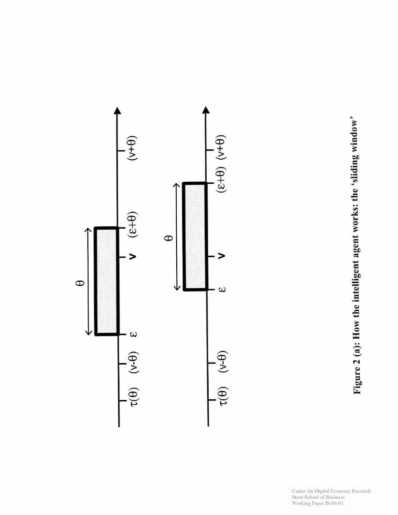
Center for Digital Economy Research Stem School of Business IVorking Paper IS-00-01

Center for Digital Economy Research Stem School of Business IVorking Paper IS-00-01
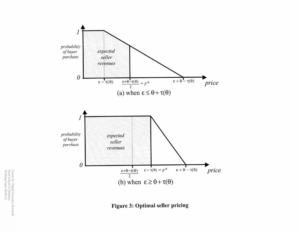
probability of buyer purchase
0 L
(a) when E 5 0 + a(0)
1
probability of buyer purchase
0 E+B-~(0) E - T ( ~ ) = P * E + @ - - T ( ~ ) price
2
(b) when E > 8 + ~ ( 8 )
Figure 3: Optimal seller pricing

Center for Digital Economy Research Stem School of Business IVorking Paper IS-00-01

Center for Digital Economy Research Stem School of Business IVorking Paper IS-00-01

Center for Digital Economy Research Stem School of Business IVorking Paper IS-00-01

Center for Digital Economy Research Stem School of Business IVorking Paper IS-00-01

Center for Digital Economy Research Stem School of Business IVorking Paper IS-00-01

Center for Digital Economy Research Stem School of Business IVorking Paper IS-00-01

$ ~ " ~ " r n r n 7 - 7 - o g g n o o o o
Center for Digital Economy Research Stem School of Business IVorking Paper IS-00-01

Center for Digital Economy Research Stem School of Business IVorking Paper IS-00-01

(a) Slow pace of IA learning (k=I) t (b) Moderate pace of IA learning (k=2) t
(b) Rapid pace of IA learning (k=3) t
Figure 11: Product choices (levels of customization) and learning rates - a closer look

Center for Digital Economy Research Stem School of Business IVorking Paper IS-00-01

Center for Digital Economy Research Stem School of Business IVorking Paper IS-00-01

Center for Digital Economy Research Stem School of Business IVorking Paper IS-00-01

I / deadweight I
(a) IA: Slow pace of learning (k=l) Vmax
Vmax
.. .. .. .. ...... fixe.d.prkc.e] ,,,,,, ,... .... .. ... , , , . . . . . . . . . . . , . . , , , . . . . . . . . . . . . , . , , , , , , , , . . . . . . . . . . . . .
(b) IA: Rapid pace of learning (k=3) vmax
(c) No IA: Fixed price vmax
Figure 15: Seller profit and buyer surplus: High cost of commiditization t