The impact of increasing carbon dioxide on ozone recovery

Joan E. Rosenfietd 1

University of Maryland Baltimore County, Baltimore, Maryland

Anne R. DouglassNASA Goddard Space Flight Center, Greenbelt, Maryland

David B. Considine

University of Maryland, College Park, Maryland

https://ntrs.nasa.gov/search.jsp?R=20010047506 2018-06-03T02:11:09+00:00Z

2

Abstract.

We have used the GSFC coupled two-dimensional (2D) model to study the impact of increasing carbon

dioxide from 1980 to 2050 on the recovery of ozone to its pre-1980 amounts. We find that the changes

in temperature and circulation arising from increasing CO2 affect ozone recovery in a manner which

varies greatly with latitude, altitude, and time of year. Middle and upper stratospheric ozone recovers

faster at all latitudes due to a slowing of the ozone catalytic loss cycles. In the lower stratosphere, the

recovery of tropical ozone is delayed due to a decrease in production and a speed up in the overturning

circulation. The recovery of high northern latitude lower stratospheric ozone is delayed in spring and

summer due to an increase in springtime heterogeneous chemical loss, and is speeded up in fall and

winter due to increased downwelling. The net effect on the higher northern latitude column ozone is to

slow down the recovery from late March to late July, while making it faster at other times. In the high

southern latitudes, the impact of CO2 cooling is negligible. Annual mean column ozone is predicted to

recover faster at all latitudes, and globally averaged ozone is predicted to recover approximately ten

years faster as a result of increasing CO 2.

;.i 3r j

3

1. Introduction

As the halogen loading of the stratosphere decreases, ozone is expected to recover to its

pre-1980 values in about 2050 (WMO, 1999). A topic of much concern is the effect that

increases in the greenhouse gas CO 2 will have on this recovery. Modeling studies have

generally agreed that increases in CO 2 will lead to a cooling of the stratosphere (e.g. Fels et

al., 1980; Rind et aL, 1990). This cooling is expected to reduce temperature dependent loss

processes, resulting in increases in upper stratospheric ozone (e.g. Brasseur and Hitchman,

1988; Pitari et al., 1992). Recently, some studies using a three-dimensional (3D) model and a

highly parameterized chemistry scheme have indicated that the stratospheric cooling due to

the build-up of greenhouse gases would lead to increases in polar stratospheric clouds

(PSCs) resulting in larger seasonal ozone depletions [Shindell et al., 1998a; Shindell et al.,

1998b]. Their proposed mechanism is a reduction of planetary wave propagation into the

stratosphere, resulting in a polar cooling. These authors suggest that ozone recovery will be

slower than expected solely from the projected decline in stratospheric chlorine loading. A

series of one-year simulations by a general circulation model with coupled chemistry [Austin et

aL, 2000] were carried out for six years during the 1979 to 2014 time period. The results

suggested that increasing greenhouse gases were delaying the onset of ozone recovery. A

survey of transient chemistry-climate experiments using four different 3D models was

summarized in WMO 1999. Three of the models showed increasing Arctic losses as a result

of increasing CO 2, while one model showed no significant changes. Of these 3D models,

however, those having full chemistry schemes were limited to runs of less than a decade.

Those 3D models capable of runs several decades long had highly simplified chemistry

schemes. Because of computational costs, long runs with interactive full chemistry and

radiation are currently limited to two-dimensional (2D) models.

4

We haveusedthe GSFCcoupledtwo-dimensional(2D) modelto studythe impactof

increasingcarbon dioxide from 1980 to 2050 on the stratospheric recovery of ozone to its pre-

1980 values. The residual circulation in the coupled model changes in response to both

radiative forcing changes and changes in the planetary wave propagation computed with a

planetary wave parameteriztion. However, tropospheric wave forcing is fixed. It is unclear how

changes in tropospheric wave forcing would alter the stratospheric circulation, and 3D models

have obtained inconsistent results on this issue [Mahfouf et aL, 1994; Butchart et aL, 2000;

Rind et al., 1990]. Thus we will focus primarily on the interactions between radiation and

chemistry, in a manner complementary to other studies of this problem [e.g., Shindell et aL,

1998]. In Section 2 we summarize the relevant model characteristics, in Section 3 we present

the results, and in Section 4 we give the summary and conclusions.

2. Model

The Goddard coupled 2D (latitude-pressure) chemistry-radiation-dynamics model is fully

interactive in temperature, ozone, and water vapor. The model has full chemistry and radiation

schemes and has been described in Rosenfield et aL [1997], with improvements given in

Rosenfield et aL [1998] and Rosenfield and Douglass [1998]. These improvements include

the use of model generated water vapor, as well as ozone and temperatures, in the radiative

heating calculation, the radiative heating due to PSCs, and the use of the Lin and Rood [1996]

scheme for the numerical advection of atmospheric trace species. Gases included in the

radiation calculation are carbon dioxide, ozone, and water vapor. Advection in the dynamics

module uses the Prather second-order moments transport scheme [Prather, 1986]. The

chemical reaction rates and photolysis cross sections used are those given in the Jet

Propulsion Laboratory (JPL) recommendation [DeMore et al., 1997].

_ 7 4

5

The model dynamics incorporates a planetary wave parameterization which propagates

waves, calculates the wave-mean flow interaction, and estimates the meridional eddy

diffusivity produced by wave dissipation [Bacmeister et al., 1995]. The planetary waves are

forced from below by topography. Thus, although there is no interannual variability in

tropospheric wave forcing, the stratospheric wave propagation and eddy mixing can respond

to temperature changes induced by increasing CO 2.

The model chemistry includes a detailed treatment of heterogeneous chemistry on

background stratospheric aerosol and polar stratospheric clouds. The condensed mass of

PSCs is calculated by integrating over an observationally based temperature probability

distribution which takes into account the longitudinal variations in temperature, as described in

Considine et aL [1994] and Rosenfield et aL [1997]. in this work the probability distribution

has been shifted to colder temperatures by 2 K, to be consistent with the present day

observed Arctic ozone losses. Particle sedimentation is included, but the effects of volcanic

aerosols have not been included in this study.

Time dependent runs used natural and anthropogenic source gas boundary conditions

given by Scenario A3 of WMO 1999. These correspond to the maximum emissions allowed

within protocols. Surface chlorine Ioadings were 2.4 ppbv in 1980, increasing to 3.6 ppbv in

1995, and declining thereafter. The model was run from 1970 through 2050, the years 1970 to

1980 being allowed for spin-up. CO 2 mixing ratios increase from 325 ppmv in 1980 to 509

ppmv in 2050. Another run was done in which all source gas boundary conditions changed

with time except for CO 2, which was fixed at its 1980 value.

3. Results

a. Global column ozone

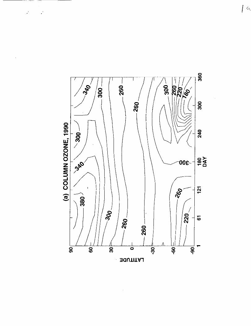
Figure 1 shows modeled 1990 column ozone as a function of latitude and day of year (Fig. la)

compared with TOMS (Fig. lb). The high latitude maximum is on the pole in the northern hemisphere

(NH) and off the pole in the southern hemisphere (SH), in agreement with observations. Column ozone

amounts are within about 10% of TOMS (Fig. lc) except in the high southern latitudes. The Antarctic

springtime ozone hole occurs about one month later than observed. This may be due to the fact that the

model cannot account for excursions of the vortex off the pole. The return of the Antarctic column ozone

to pre-springtime values is slower in the model than in observations. This is likely due to insufficient high

latitude meridional mixing at the time of vortex breakup.

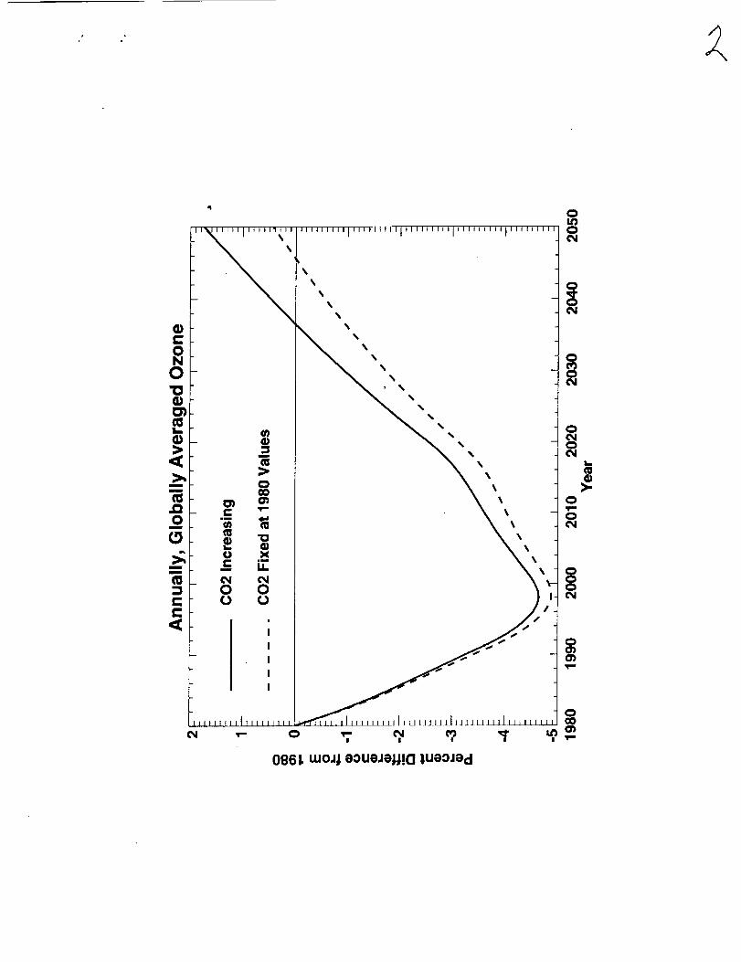
Figure 2 shows the differences from 1980 of annually, globally averaged column ozone amounts for

the increasing and fixed CO 2 simulations. For both simulations minimum ozone amounts are reached in

1998, followed by a recovery which is slower for the fixed CO2 case. Increasing CO2 is seen to speed

up the recovery to 1980 values by approximately ten years, with the fixed CO2 ozone recovering in the

year 2046 and the increasing CO 2 ozone recovering in the year 2037.

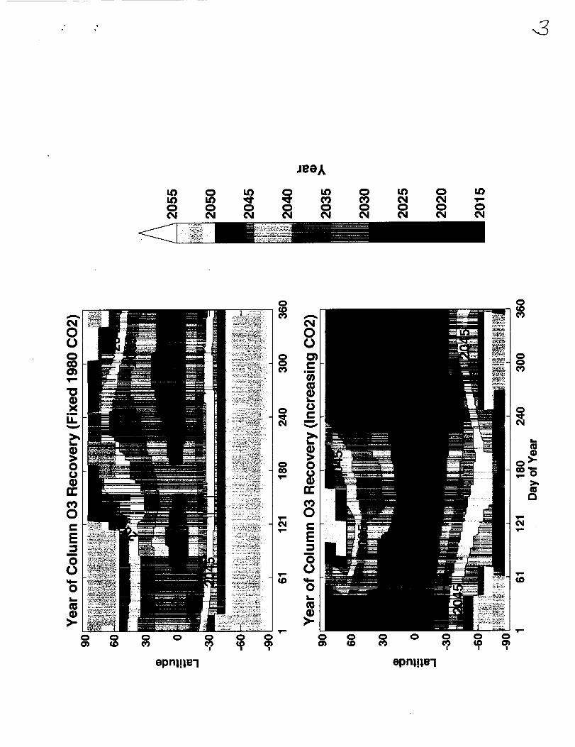
Figure 3 shows the year of recovery of column ozone to 1980 values as a function of day of year and

latitude. Increasing CO 2 speeds up the recovery of column ozone in all seasons in the low and middle

latitudes. Recovery is fastest in the tropics, with a speedup due to increasing CO 2 of between 5 and 10

years. In the middle latitudes, the speedup in recovery with increasing CO2 is greatest in the fall and

winter months. In the polar latitudes, increasing CO2 speeds up NH recovery in the fall and winter and

slows it down in spring and early summer, and speeds up SH recovery in the fall and winter. Annual

mean column ozone recovers faster at all latitudes (not shown). We present the results in more detail in

the following two sub-sections.

,_ r _

7

b. Tropics

As seen in Figure 3, the computed effect of increasing CO2 on low latitude column ozone recovery

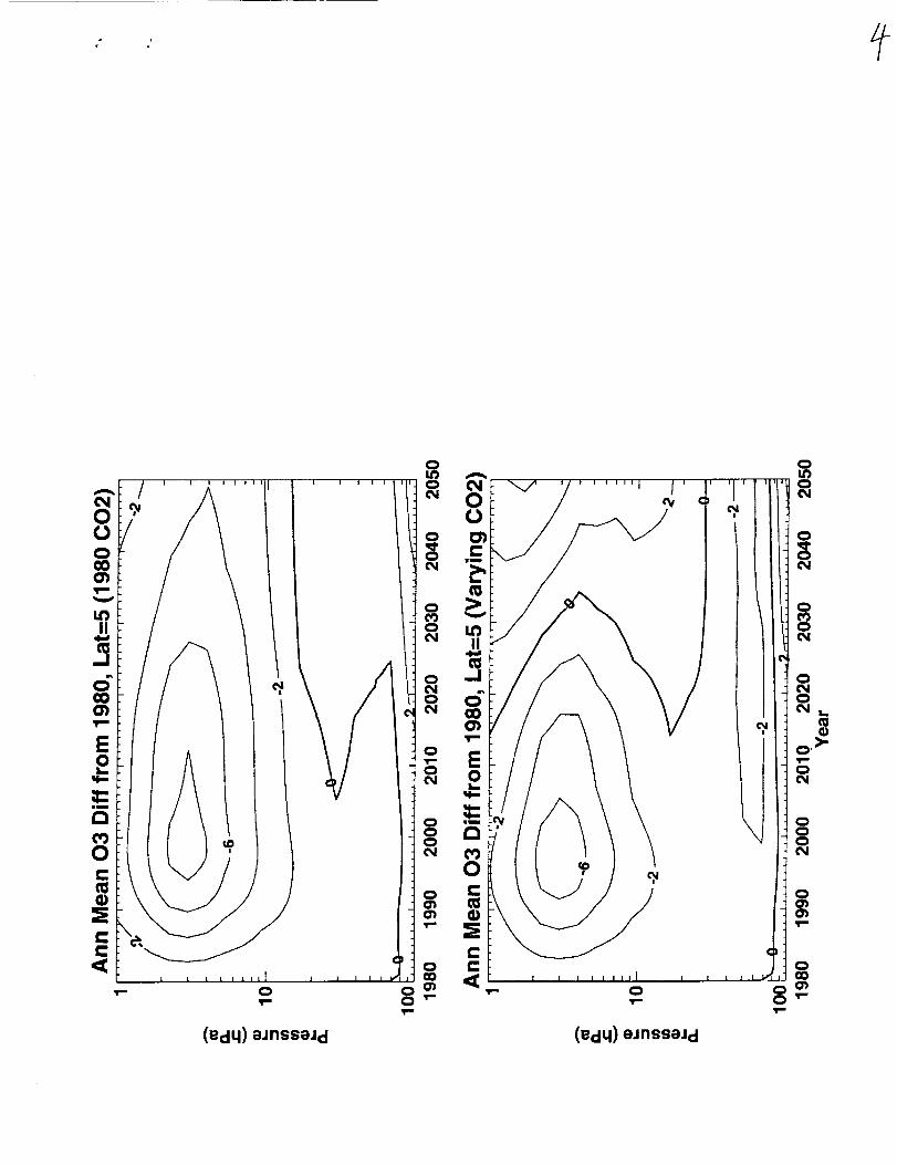
shows relatively little seasonal variability. We therefore focus on the annual mean results. Figure 4

shows annual mean ozone mixing ratio differences from 1980 at 5N as a function of year and pressure.

There is a faster recovery with increasing CO2 above about 30 hPa. Below 30 hPa there is no recovery

out to year 2050 in the increasing CO 2 case. The net effect on the column ozone amount is a faster

recovery.

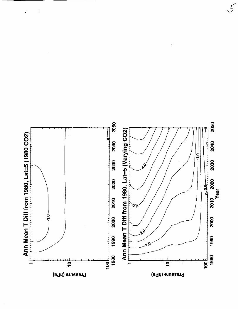
To understand the differing behavior with altitude, we need to examine the changes in temperature,

vertical velocity, and ozone chemical production and loss. Figure 5 shows annual mean temperature

differences from 1980 as a function of year and pressure at 5N. With fixed CO2, reductions in upper

stratospheric temperatures on the order of 0.5 - 1 K are computed. This cooling is due to decreased

solar heating as a result of ozone losses. With increasing CO s, an increase in infrared cooling leads to a

cooling of the stratosphere. Upper stratospheric temperatures drop by more than 5 K by the year 2050.

The upper troposphere is computed to warm by less than 1 K. The feedback of the computed ozone

changes on the heating rates results in smaller absolute temperature changes than would be computed

without this feedback.

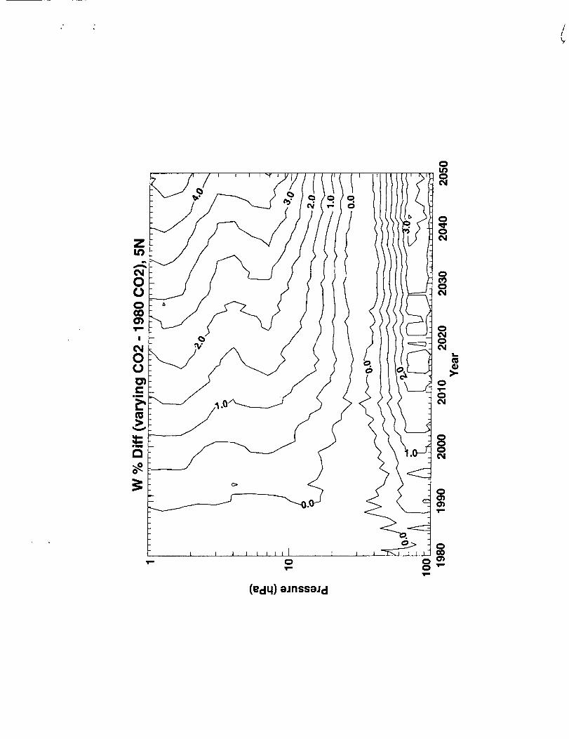
Vertical velocity differences between the varying CO2 run and the fixed CO s run at 5N are shown in

Figure 6. As has been shown before in a doubled CO2 experiment, increasing CO2 will increase the

residual circulation in the middle and upper stratosphere (e.g., Rosenfield and Douglass, 1998). In this

study the increase in tropical upper stratospheric vertical velocities reaches a maximum of 5% in the

year 2050. In the lower stratosphere the increasing CO2 leads to a 2-3% increase in vertical velocity

maximizing at 70 hPa after the year 2010. Lower temperatures increase the modeled infrared heating

which is greater than the solar heating in 16-18 km region.

The computed chemical loss frequencies for the various gas phase catalytic destruction cycles are

shown in Figure 7 for the year 1980. Figure 8 shows the change of 2020 loss frequencies from 1980,

with and without changing CO 2. Throughout most of the stratosphere the cooling due to increasing CO2

8

leadsto a reductionin thelossfrequenciesforeachofthecycles.Thesereductionscanbeattributedto

botha directeffectandindirecteffectsofcooling.A directeffectofcoolingis thewellknownslowingof

theozonerecombinationreactionO+03 -> 2 02,whoserateconstantisproportionalto exp(-2060/T).

Thisexplainsthereductionofthe lossfrequencydueto theOxcycle.Theratedeterminingstepsof the

remaininglosscyclesdonothavea largetemperaturedependence.

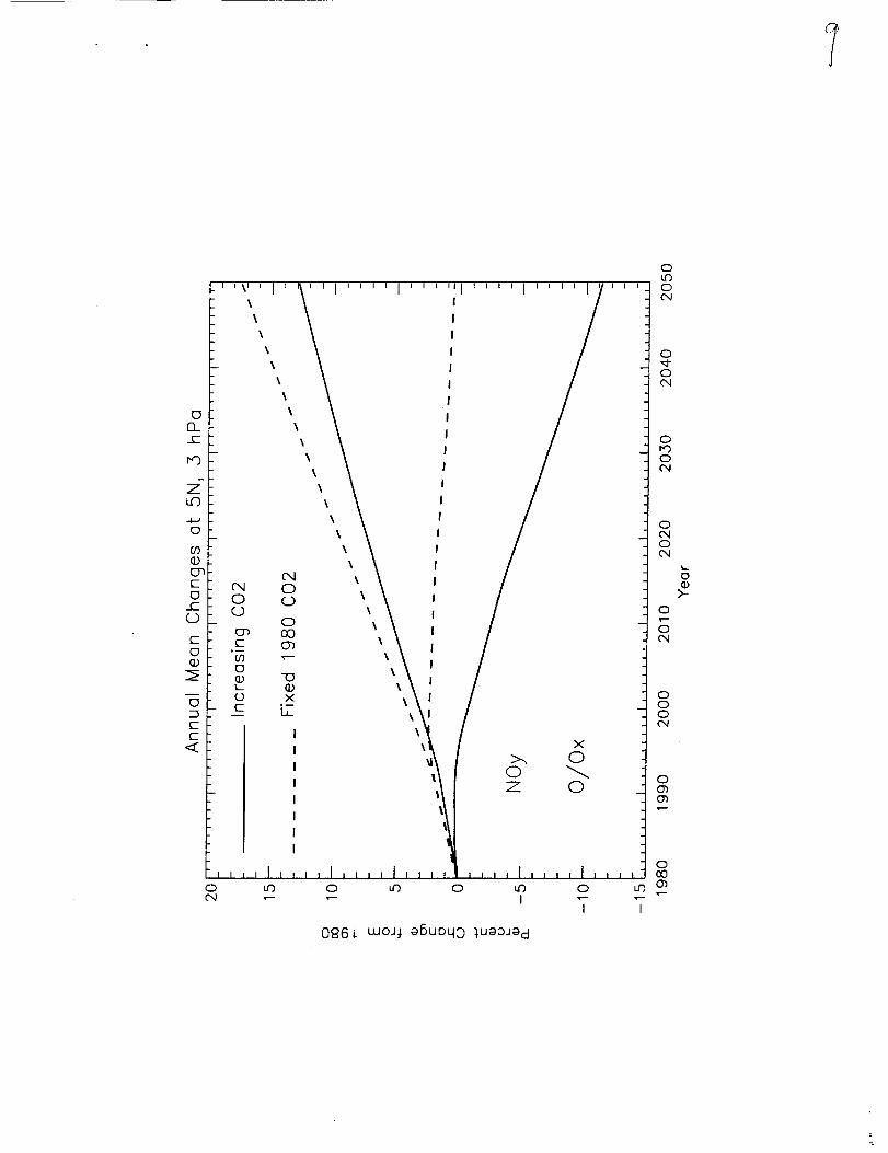
Indirecteffectsof coolingarea decreaseinNOyandadecreasein theO/Oxratio. Computed

changesinupperstratosphericNOyandtheO/Oxratioforthe1980to 2050periodareshownin Figure

9. NOyis increasingwithtimebecauseofthe increasingabundanceofthegreenhousegasN20.

However,theincreaseinNOyis lesswhenonetakesintoaccountthecoolingdueto C03increases.A

reductioninNOywithcoolinghasbeenshown[Rosenfieldand Douglass, 1998] to arise from the very

large temperature dependence of the reaction N + 02 -> NO + O (k~exp3600/T]). The abundance of N

is increased with cooling, leading to an increase In the loss of NOy which is controlled by the reaction N

+ NO -> N2 + O. This decrease in NOy contributes to the reduction of the ozone loss frequency due to

the NOx cycle.

The O/Ox ratio changes very little with time when CO 2 is fixed, while decreasing markedly when CO2

cooling occurs. This decrease with cooling of the O/Ox ratio results from a change in the 0/03

partitioning, which is controlled by the reaction O + 02 + M -> 03 + M. The rate constant for this

reaction is proportional to [300/m]2"3. This decrease of O/Ox contributes to the slowing of all the ozone

catalytic loss cycles with cooling. Since NO x dominates at 30-2 hPa, a slowdown of NO x loss has the

largest impact.

In the middle and upper stratosphere, the chemical loss term dominates the transport term in the

ozone tendency equation. We can thus attribute the faster recovery of tropical ozone mixing ratios

above -30 hPa to the slowing of the chemical loss cycles with cooling. While ozone increases in the

tropical middle and upper stratosphere have been noted before as a result of increasing C03 [e.g. Rind

et aL, 1998], we have shown using our detailed chemistry scheme that these increases are attributable

to a combination of changes in both NOy amounts and partitioning within the Ox species. In the tropical

9

lowerstratospheretheozone loss is dominated by the HOx catalytic cycle, which shows a small change

with cooling which changes sign at 70 hPa. Lower stratospheric ozone production, however, is computed

to be reduced by roughly 2% due to the effects of the middle and upper stratospheric ozone increases

on 02 photolysis rates. This is the reverse of "self-healing", an increase in lower stratospheric tropical

ozone calculated as a result of upper stratospheric losses due to increased chlorine [Hudson, 1977,

p.201]. We thus attribute the delayed recovery of lower stratospheric ozone to the combined effects of

decreased production and increased upwellingo The middle and upper stratospheric changes outweigh

those of the lower stratosphere, leading to a faster recovery of the column.

C. Extra-tropics

At high latitudes, lower stratospheric cooling is expected to cause increases in PSCs and a potential

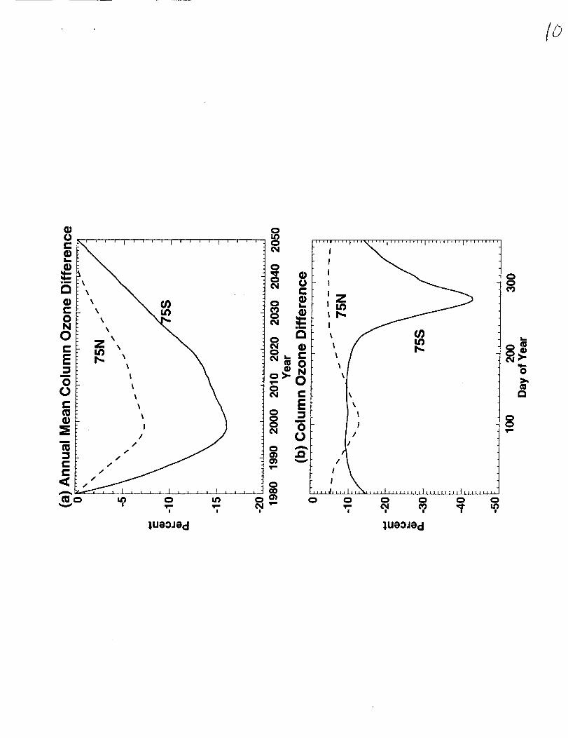
enhancement of springtime ozone destruction. Figure 10 (top) shows the computed annual mean column

ozone differences from 1980 as a function of year at 75N and 75S, for the increasing CO2 case. The

maximum depletions relative to 1980 occur during the years 1998-2000. Figure 10 (bottom) shows the

1998-2000 mean column ozone differences, relative to 1980, at 75N and 75S as a function of day of

year. Maximum springtime depletions of -42% and -12% are computed in October at 75S and in April

at 75N, respectively. Observations show that the lowest ozone values occur about one month earlier

than computed, in March and September for the NH and SH, respectively. We have seen in Figure 1

that the Antarctic ozone hole occurs later in the model than observations. As a comparison, TOMS 70-

80N zonal mean differences for the March 1998-2000 average relative to the March 1979-1980 average

are -9.4%. The corresponding TOMS differences at 70-80S in September are -40%.

A major contributor to the springtime column ozone losses are lower stratospheric decreases of ~20-

25% in the NH and 90-100% in the SH (not shown). These losses are due to the activation of chlorine

as a result of heterogeneous reactions occurring on the surfaces of PSCs. As mentioned in Section 2,

the temperature probability distribution used in the computation of PSC amounts was shifted to slightly

colder temperatures to ensure the approximate agreement of computed with observed present day

10

ozonedepletions.Attheonsetof spring,computed lower stratospheric chlorine activation is roughly 30-

40% at 75N and close to 100% at 75S.

Associated with the computed chlorine activation is denitrification. At 75S, model computed NOy in the

1998-2000 winter is -90% less than that computed in a run with no heterogeneous chemistry. Moderate

denitrification of -30-40% is computed at 75N. Evidence for moderate Arctic denitrification has been

observed in years with cold stable Arctic vortices [Rex et aL, 1999; Santee et aL, 2000; Fahey et aL,

2001].

We turn now to the effects of increasing CO2 on the recovery of high latitude ozone. As shown in

Figure 3, the effect of changing CO2 on column ozone in the high northern latitudes depends on the time

of year. Column ozone recovers to its 1980 values slower from late March to late July while recovering

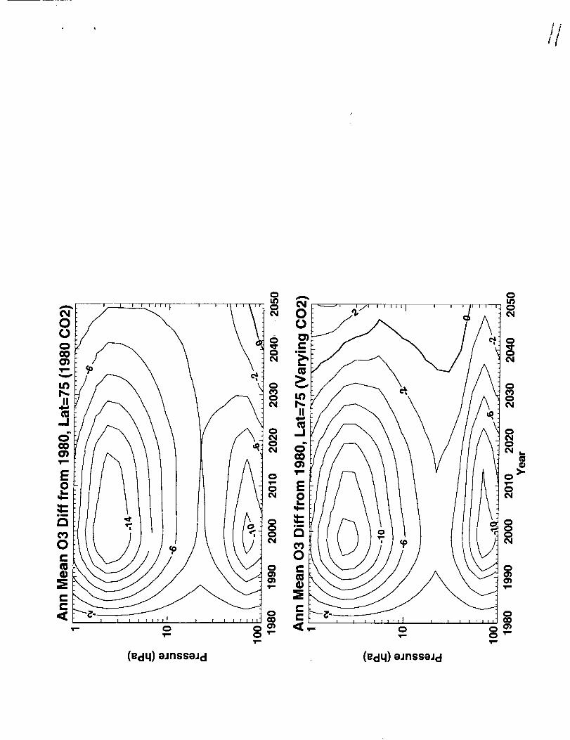
faster the rest of the year. In the annual mean the column recovery is faster with increasing CO2. Figure

11 shows the annual mean ozone profile differences from 1980 at 75N. Above about 50 hPa, where

approximately 43% of the total column resides, the recovery is faster with increasing CO2, while below it

is slower. The faster recovery above 50 hPa occurs throughout the year, and the same reasons hold as

did for the tropical upper stratosphere - i.e. the lowered NOy and O/Ox due to colder temperatures slow

the gas phase ozone destruction reactions.

The slower recovery of ozone in the high northern latitude lower stratosphere is a result of increasing

springtime heterogeneous loss. Figure 12a shows computed ozone mixing ratios throughout the year

2020 at 75N and 68 hPa. Ozone amounts start declining from their late winter high values in March,

reaching their lowest values in late August, after which downwelling brings down air containing higher

ozone amounts.

With increasing CO2 there is a faster decline in March and April, and a slower decline from May

through August (Fig. 12b). During March and April between -40-70 hPa there is a 20-35% increase in

the chlorine catalyzed loss arising from increased heterogeneous processing. A 1-2 K cooling leads to

an increased amount of PSCs and denitrification. For example, maximum amounts of Type I PSCs at 68

hPa in the year 2020 increase 43%, and late winter to early spring denitrification increases from 35% to

11

about45%withcooling. Computed Type II PSCs are negligible in the high northern latitudes. Although

HCI mixing ratios are very small in both cases due to the HCI + CIONO 2 -> CI2 + HNO3 reaction, the

increase in surface area and the colder temperatures allow the CIONO 2 + I-_O -> HOCI + HNO3 reaction

to be more important. This explains the greater spring ozone loss due to the chlorine catalytic cycle.

After April, ozone loss is controlled by the gas phase processes. From late spring through summer the

net ozone loss frequency is less for the increasing CO2 case, mainly due to a reduction in the NOx cycle

as a result of lower NOy. In fall and winter an increase in downwelling in the changing CO 2 case results

in higher values of ozone.

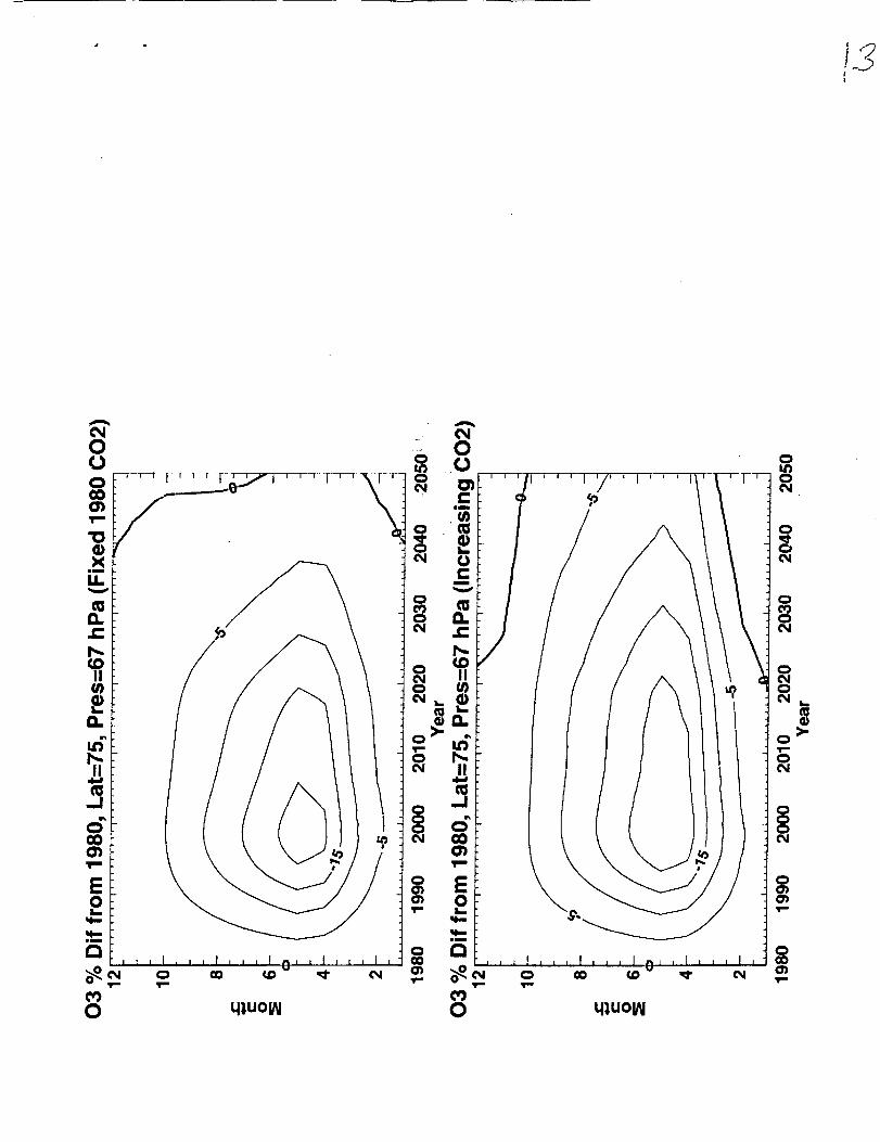
Figure 13 shows ozone differences from 1980 at 75N and 68 hPa as a function of year and month.

After springtime ozone reaches its lowest levels in approximately the year 2000, the beginnings of

recovery occur roughly ten years later in the increasing CO2 case. At this level the ozone recoven/to

its 1980 values is slowed down between March and October and speeded up at other times.

In the southern high latitudes, computed column ozone recovers faster throughout the year with

increasing CO 2 (not shown). In the middle and upper stratosphere the faster recovery is due to the

reduction in NOy and O/Ox, which slows down the gas phase loss reactions. In the lower stratosphere,

ozone has a faster recovery during fall and winter months due to increased downwelling. The impact on

springtime lower stratospheric ozone depletion is negligible. Although additional cooling results in the

formation of higher amounts of Type I PSC, chlodne activation is already nearly complete and ozone

loss nearly 100% in the fixed CO2 case.

The planetary wave parameterization included in the model formulation allows for the computation of

horizontal eddy mixing. This results in some mixing of the high latitude springtime ozone depletions into

the middle latitudes, thus slowing the northern middle latitude ozone recovery below about 40 hPa for

some seasons. For example, at 45N and 68 hPa, increasing CO2 causes ozone recovery to be slowed

down from April to October. The middle and upper stratospheric speed up in ozone recovery dominates,

resulting in a faster recovery of column ozone in the middle latitudes.

12

4. Summary and Conclusions

Our 2D coupled model results show that both direct and indirect feedbacks affect the global

distribution of ozone. The changes in temperature and circulation arising from increasing CO2 affect

ozone recovery in a manner which varies greatly with latitude, altitude, and time of year. Firstly, the

stratospheric cooling due to increasing CO2 feeds back on the temperature dependent homogeneous

reaction rates. This affects ozone loss rates both directly and indirectly, resulting in a slowing of all the

ozone catalytic loss cycles in the middle and upper stratosphere. Ozone is predicted to recover to 1980

values faster throughout the year above -30 hPa in the tropics and above -50 hPa in the extra-tropics,

with increasing CO2. Secondly, in the tropics below -30 hPa, ozone recovery is predicted to be slowed

down by both a decrease in production and an increase in upwelling.

In the high latitude northern lower stratosphere, ozone recovery is predicted to be slowed down in

spring and summer due to an increase in springtime heterogeneous chemical loss due to the CO2

cooling. Some of this increased high northern latitude chemical loss is mixed into the middle latitudes. In

the high southern latitudes, the impact of CO2 cooling is negligible. High latitude lower stratospheric

ozone recovery is predicted to be hastened in the fall and winter by an increase in downwelling.

In the annual mean, column ozone is predicted to recover faster at all latitudes with increasing CO2. In

the tropics the column ozone recovers faster in all seasons, while in the high northern latitudes, column

ozone recovery is slowed clown from late March to late July and speeded up the rest of the year. In the

global mean, the increasing high northern latitude ozone depletion caused by the increase in PSCs

calculated in a cooler lower stratosphere is outweighed by ozone increases at higher altitudes and lower

latitudes. As a result, the model results suggest that increasing CO 2 will hasten the recovery of globally

averaged column ozone by approximately ten years.

The model planetary wave scheme includes the effects of dynamical changes in the stratospheric

planetary wave propagation. Shindell et al. [1996a] noted that the refraction of planetary waves into the

tropics as a result of greenhouse gas cooling reduced the frequency of stratospheric warmings and

exacerbated polar cooling. Our model includes these processes in a parameterized way, but we find the

13

changes in wave propagation to be negligible. We note that 3D models do not agree on this point

[Mahfouf et aL, 1994; Butchart et aL, 2000]. Much colder lower stratospheric temperatures, whether

caused by dynamical changes which we cannot model in a 2D framework or other causes, would result

in an increase in NH high latitude heterogeneous processing. The effect on ozone recovery in the

middle latitudes and thus globally averaged ozone recovery would depend on the extent to which the

high latitude depletions mix to lower latitudes. In the absence of significant changes in tropospheric

wave forcing, a purely radiative cooling of the stratosphere due to increasing CO2 leads to a faster

recovery of the global average ozone.

Acknowledgments. We thank Paul Newman, Julio Bacmeister, Mark Schoeberl, and Rich Stolarskifor helpful comments.

1Mailing address: Code 916, NASA Goddard Space Flight Center, Greenbelt, MD 20771(rose@euterpe.gsfc.nasa.gov)

14

References

Angell, J. K., Difference in radiosonde temperature trend for the period 1979-1998 of MSU data and the

period 1959-1998 twice as long, Geophys. Res. lett., 27, 2177-2180, 2000.

Austin, J., J. Knight, and N. Butchart, Three-dimensional chemical model simulations of the ozone layer:

1979-2015, Q. J. R. MeteoroL Soc., 126, 1533-1556, 2000.

Bacmeister, J.T., M.R. Schoeberl, M.E. Summers, J.E. Rosenfield, and X. Zhu, Descent of long-lived

trace gases in the winter polar vortex, Jo Geophys. Res., 100, 11,669-11,684, 1995.

Brasseur, G., and M. Hitchman, Stratospheric response to trace gas perturbations - changes in ozone

and temperature distributions, Science, 240, 634-637, 1988.

Butchart, N., J. Austin, J.R. Knight, A.A. Scaife, and M.L. Gallani, The response of the stratospheric

climate to projected changes in the concentrations of well-mixed greenhouse gases from 1992 to 2051,

J. Climate, 13, 2142-2159, 2000.

DeMore, W. B., Chemical kinetics and photochemical data for use in stratospheric modeling, Evaluation

number 12, JPL PubL, 97-4,266 pp., 1997.

Fahey, D.W., et al., The detection of large HNO3-containing particles in the winter

arctic stratosphere, Science, 291, 1026-1031, 2001.

Fels, S.B., J.D. Mahlman, M.D. Schwarzkopf, and R.W. Sinclair, Stratospheric sensitivity to perturbations

in ozone and carbon dioxide: radiative and dynamical response, J. Atmos. ScL, 37, 2256-2297, 1980.

Hudson, R.D. (Ed.), Chlorofluoromethanes and the stratosphere, NASA Ref. PubL 1010, 266 pp., 1977.

Lin, S.-J., and R.B. Rood, Multidimensional flux-form semi-Lagrangian transport schemes, Mon. Weather

Rev., 124, 2046-2070, 1996.

Mahfouf, J.F., D. Cariolle, J.-F. Royer, J.-F. Geleyn, and B. Timal, Response of the Meteo-France

climate model to changes in CO 2 and sea surface temperature, Clim. Dyn., 9, 345-362, 1994.

Pawson, S., K. Labitzke, and S. Leder, Stepwise changes in stratospheric temperature, Geophys. Res.

Lett., 25, 2157-2160, 1998.

Pawson, S., and B. Naujokat, The cold winters of the middle 1990s in the northern lower stratosphere, J.

r' ,°

15

Geophys. Res., 104, 14,209-14,222, 1999.

Pitari, G., S. Palermi, and G. Visconti, Ozone response to a CO2 doubling: Results from a stratospheric

circulation model with heterogeneous chemistry, J. Geophys. Res., 97, 5953-5962, 1992.

Prather, M.J., Numerical advection by conservation of second-order moments, J. Geophys. Res., 91,

6671-6681, 1986.

Rex, M., et al., Subsidence, mixing, and denitrification of Arctic polar vortex air measured during

POLARIS, J. Geophys. Res., 104, 26,611-26,623, 1999.

Rind, D., R. Suozzo, N.K. Balachandran, and M.J. Prather, Climate change and the middle atmosphere.

Part I: The doubled CO2 climate, J. Atmos. ScL, 47, 475-494, 1990.

Rind, D., D. Shindell, P. Lonergan, N.K. Balachandran, Climate change and the middle atmosphere. Part

II1: The doubled CO2 climate revisited, J. Climate, 1I, 876-894.

Rosenfield, J. E., et al., Stratospheric effects of Mount Pinatubo aerosol studied with a coupled two-

dimensional model, J. Geophys. Res., 102, 3649-3670, 1997.

Rosenfield, J. E., et al., The impact of subvisible cirrus clouds near the tropical tropopause on

stratospheric water vapor, Geophys. Res. Lett., 25, 1883-1886, 1998.

Rosenfield, J. E. and A. R. Douglass, Effects on NOy in a coupled 2D model, Geophys. Res. Lett., 25,

4381-4384, 1998.

Santee, M. L., G. L. Manney, N. J. Livesey, and J. W. Waters, UARS Microwave Limb Sounder

observations of denitrification and ozone loss in the 2000 arctic late winter, Geophys. Res. Lett., 27,

3213-3216, 2000.

Shindell, D.T., D. Rind, and P. Lonergan, Increased polar stratospheric ozone losses and delayed

eventual recovery owing to increasing greenhouse-gas concentrations, Nature 392, 589-592, 1998a.

Shindell, D.T., D. Rind, and P. Lonergan, Climate change and the middle atmosphere. Part IV: ozone

response to doubled CO 2, J. of Clim., 11, 895-918, 1998b.

WMO, Scientific Assessment of Ozone Depletion: 1998, Rep. No. 44, Geneva, 1999.

°"

16

FIGURE CAPTIONS

Figure 1. (a) Computed column ozone (DU) in 1990 as a function of day of year and latitude. (b) TOMS

column ozone (DU) averaged for the years 1988-1992 as a function of day of year and latitude. (c)

Percent difference of computed from TOMS column ozone. The model year has 360 days.

Figure 2. Time series of percent difference of annually, globally averaged ozone from 1980. Solid line is

increasing CO 2 case, and dashed line is fixed CO2 case.

Figure 3. (top) Year of column ozone recovery to 1980 values as a function of day of year and latitude

for fixed CO 2 case. (bottom) Same as top except for increasing CO2 case. The model year has 360

days.

Figure 4. Computed percent differences of annual mean ozone mixing ratios from 1980 values at 5N

with (top) CO 2 fixed at 1980 values and (bottom) CO 2 increasing.

Figure 5. Computed annual mean temperature differences from 1980 at 5N with (top) CO2 fixed at 1980

values and (bottom) CO 2 increasing.

Figure 6. Computed percent differences of annual mean vertical velocities at 5N for the increasing CO2

case compared with the fixed CO2 case.

Figure 7. Computed 1980 annual mean Ox loss frequencies at 5N.

Figure 8. Computed percent differences of annual mean Ox loss frequencies (2020 - 1980) at 5N. Solid

lines refer to increasing CO2, while dashed lines refer to fixed 1980 CO2.

Figure 9. Percent changes of annual mean NOy and O/Ox at 5N and 3 hPa. Solid lines refer to the

increasing CO 2 case, while dashed lines refer to fixed CO 2 case.

Figure 10. (a) Computed percent difference of annual mean column ozone from 1980 at 75S (solid) and

75N (dashed), for the case of increasing CO2; (b) computed percent difference of 1998-2000 mean

column ozone from 1980 at 75N (dashed) and 75S (solid), for the case of increasing CO2.

Figure 11. Computed percent differences of annual mean ozone mixing ratios from 1980 values at 75N

with (top) CO 2 fixed at 1980 values and (bottom) CO 2 increasing.

Figure 12. (a) Computed ozone mixing ratios in the year 2020 at 75N and 67 hPa for increasing CO2

o' I I

(solid) and fixed 1980 CO2 (dashed). Tick ma,ks a_ at the middle of the months. (b) Difference of

ozone mixing ratios in 2020 at 75 N and 67 hPa (increasing CO 2 minus fixed CO2 case).

Figure 13. Computed percent differences of ozone mixing ratios at 75N and 67 hPa from 1980 values

with (top) CO 2 fixed at 1980 values and (bottom) CO2 increasing.

"_7

I Ct

30N.LI/V1

0_DO3

00O3

0

e_"-a

o o o o

3an.l.liVl

o o oI ! !

3ClrlII.LV-I

C0N0

m

>

in

m

oI

im

m

e-e-'

0

0

0

0_N

0

004

0

0tN

lillllllltIIIIIll_

0II I

086 L uJoJJ aouoJatJ!O ),ugoJOd

0

0O)

,li

000

1._.

>-

JeoA

AC_I0oo_0O_

xulml

U..

>,

0U

rr030

E0

U

o otD

i ! !

epn|p.e'l

o

wm

C_0e-

Ce-<C

/

0

'I"

0

IN

00IN

(edq) eJnsse.ld (edq) eJnsseJd

I-

<i

I I I IIII I I

0

(edq) eJnsseJd (edq) eJnsseJd

0

0

0

(edq) oJnssoJd

7

I I I I I 0 I l I

II

I II

I I I I Ill

0

(edq) eJnsseJd

Z

Zt I I I I

%%

%

X X_x O OU -r Z

I I I I !

(gdq) emsseJd

%%

0U0O0

I

I

I

I

I

I

I

I I I

o I

o0

0a3(_

-O_)x

\\

\

\

\

I

I

I

I

I

I

0Z

x0

0

oi._oc_

o

o(N

01,0o('4

ocwo(N

0

0

oo0c,q

o0_

>-

0cN

Lr) o LD 0 L.O 0

/

Og6L woJ_ aBuoq3 luaaJa d

ooo

u30_

I

/0

\\

Z \\\

I

IJ

luaoJad luaoJad

//

(edq) eJnsseJd (edq) eJnss_Jd

Atudd

z

0

r=.-j ,.0=,

c-o

14.

A

o

e-

=o

Ul

CZ

0

A

,o,,',,,_,==

q_uol_

_1 qll

0 q_,u01_

o

oo

o

o_