The Impact of High School Leadership on Subsequent Educational Attainment*

Kathryn Rouse, Ph.D., Elon University

December 2010

*Direct correspondence to Kathryn Rouse, Department of Economics, Elon University, Elon, NC 27244 (krouse@elon.edu). Earlier versions of this paper were presented at the Eastern Economics Association and Midwest Economics Association Annual Meetings. I would like to thank Tom Mroz, David Blau, Donna Gilleskie, David Guilkey, and Helen Tauchen for their helpful comments and suggestions. All errors are my own. This study uses restricted-use data provided by the NCES.

Abstract

Objectives: Universities increasingly emphasize the importance of leadership skills, but budget

shortfalls in public high schools threaten the availability of leadership opportunities for many

youths. Few studies, however, have examined the impact of high school leadership experience on

key economic outcomes. This study narrows this gap by estimating the causal impact of leadership

in high school on educational attainment measured several years later. Methods: The paper uses data

from the National Education Longitudinal Study. To address selection bias, the effect of high

school leadership is estimated using ordinary least squares, propensity score matching and

instrumental variables models. Results: Every estimation method and model specification examined

implies that high school leadership has a large, positive impact on post-secondary educational

attainment. Conclusions: This paper indicates the impact of high school leadership is, at a minimum,

non-trivial. This result implies decisions regarding financial cutbacks for extracurricular activities

should not be taken lightly.

1

Introduction

Several studies have established a positive correlation between participation in athletic and

other extracurricular activities and outcomes such as academic achievement [Lipscomb (2006),

Leeds, Miller, and Strull. (2007)] and future wages [Ewing (1995); Barron, Ewing and Waddell

(2000); Eide and Ronan (2001); Stevenson (2006); Ewing (2007)]. Universities have recently started

placing a greater emphasis on leadership skill both in their selection process and in their curricula;

suggesting students not simply join every club, but also demonstrate commitment by undertaking a

leadership role [Tomsho (2009), Stone (2010)]. The limited scholarly research on leadership supports

this assertion. Kuhn and Weinberger (2005) find leadership skill is associated with higher earnings,

while Lozano (2008) provides the first piece of evidence suggesting some of this earnings premium

may come through increased educational attainment. The drawback of the current literature is that

the analyses rely primarily on regression analysis, making causal inferences difficult. Establishing a

causal link is particularly important given the fact that widespread budget shortfalls in public high

schools now threaten the availability of leadership opportunities for many youths. Some school

systems have gone as far as eliminating these activities all together [Staples (2009), Popke (2009)].

Other districts have implemented “pay-to-play” programs where, in order to participate, students

must pay a fee, typically ranging from $75 to $100 per activity [Brady and Glier (2004), Brown

(2002), Fahey (2007), Stern (2010)]. Such policies have led to heated debates with little evidence to

support either side.

This paper contributes to the literature using data from the National Education Longitudinal

Study of 1988 (NELS) to estimate the causal impact of high school leadership on educational

attainment measured eight years later. This paper improves upon prior literature by using two

additional estimation approaches to explicitly control for the potential bias that arises due to the

non-random selection of students into leadership positions. A baseline model is first estimated

2

parametrically by ordinary least squares (OLS). Then, the linearity assumption is relaxed and the

model is estimated via a propensity score matching (PSM) approach. Finally, instrumental variables

(IV) estimation is used to address directly the endogeneity of high school leadership that arises when

there is selection on characteristics that are not observed (by the econometrician).

Every estimation method and model specification examined implies that high school

leadership has a large, positive impact on post-secondary educational attainment. The most

conservative estimates suggest that students who are leaders in high school complete 0.35 more

years of education than their non-leader peers. In addition, high school leadership is predicted to

increase the probability of attending a post-secondary institution by at least five percent and to

increase the probability of holding a college degree by 9.5 percent. Leadership is also predicted to

increase the likelihood of attending a four-year school (versus two-year school) first. Similar to

many empirical studies on the return to schooling, instrumental variables estimates are larger than

the corresponding OLS and PSM estimates. Taken as a whole, the evidence in this paper indicates

that the impact of high school leadership is, at a minimum, non-trivial and suggests that the effect

may be much larger for some students.

Conceptual Framework and Previous Research

High school leadership may help develop a student’s leadership skill and increase his stock

of noncognitive human capital, and may therefore be placed within the conceptual framework of

Gary Becker’s (1964) theory of human capital. The model hypothesizes that the role of education is

as an investment in an individual’s human capital stock, or his productive skills. The costs to the

student include his forgone wage as well as any tuition or other pecuniary costs associated with his

education. The “return” on this investment comes in the form of higher wages once the individual

enters the labor market. Likewise, the experiences provided by a high school leadership position

may help to increase an individual’s leadership skill. Since this skill is sought out by academic

3

institutions and is considered a productive asset, taking on a leadership position in high school may

be viewed as investment in psychological or noncognitive human capital, which will lead the student

to not only attend college, but may also make it more likely that the student will graduate if this skill

translates into more college success. The student’s costs of high school leadership include the cost

of time in terms of his forgone leisure, study time and/or high school employment, any pecuniary

costs (e.g. participation fees), as well as the psychological costs (such as speaking in front of other

students) associated with undertaking such a position. Alternatively, since leadership positions

require a time commitment, students may substitute leadership time for study time. Thus, even if

leadership skill is increasing, if this benefit comes at the expense of diminished academic skills, high

school leadership may not have any impact or could even lead to decreased educational attainment.

Given the role that high school leadership activities play in the college admissions process,

leadership may also be placed in the framework of Michael Spence’s (1973) signaling model. In this

model, education is thought to serve as a signal to employers of an individual’s innate intelligence.

Similarly, high school leadership serves as a signal of one’s leadership ability to university admission

committees. Individuals with innately higher leadership ability and a desire to go to college may take

on leadership positions in order to separate themselves from their non-leader peers in the college

admissions process. It is therefore more likely that high school leaders will attend college and attain

a higher level of education than their non-leader peers.

To date, there has been little research on the specific impacts of high school leadership

experience. Several studies have, however, examined the economic effects of high school

extracurricular participation. Using the National Longitudinal Study of Youth 1979 (NLSY), Ewing

(1995) finds that high school athletic participation increases the wages of black males by 8 to 11

percent. Barron, et al. (2000) formalize the possible connection between athletics and human

capital, arguing that participation in high school athletics may increase traits such as self-discipline,

4

motivation and competition, which are subsequently rewarded in the labor market in the form of

higher wages. The authors test their model using data from the NLSY and the National

Longitudinal Study of 1972 (NLS-72) to examine the effects of high school athletic participation on

education and labor market outcomes of males. They find some evidence of a positive impact of

high school athletic participation on the wages and educational attainment of males; however the

effects are small when instrumental variables are used.

Using the HS&B and instrumenting athletic participation with height, Eide and Ronan

(2001) find high school athletic participation has a negative effect on the wages of white males and a

positive effect on the wages of black males and females. However, IV estimates are not significant.

More recently, Stevenson (2006) uses state variation in the athletic participation of males along with

Title IX legislation to instrument for female athletic participation. Results imply female high school

athletic participation leads to higher educational attainment, increased labor force participation and

increased participation of females in traditionally male-dominated careers.

Prior research also suggests that participation in sports and other activities (e.g. student

government, service clubs, academic clubs, etc.) does not come at the expense of academic

achievement as the time constraint theory may suggest. Using a student fixed-effects approach,

Lipscomb (2006) finds that participation in either clubs or sports is associated with an increase in

students’ high school math and science test scores as well as their Bachelor’s degree expectations.

Leeds (2003) develops a formal model that suggests athletic success has led to black men

overinvesting in athletics and underinvesting in academics. This model is adapted and tested in

Leeds et al. (2007). The authors find no evidence that athletics has a negative impact on black men

and some evidence that involvement in athletics has a positive impact on academics of white men.

In contrast to participation that may increase and signal a wide range of non-cognitive skills,

holding a leadership position specifically fosters and signals the skill of leadership - a skill that is

5

widely valued and specifically sought after by universities and employers [Tomsho (2009), Stone

(2010), Kuhn and Weinberger (2005)]. The impact of leadership on future outcomes may therefore

be more direct than simple participation. Evidence provided by Kuhn and Weinberger (2005) and

Lozano (2008) suggest that this is the case. Using data from Project TALENT, the NLS-72 and the

sophomore cohort of HS&B, Kuhn and Weinberger (2005) find white men who held leadership

positions in high school earn 4% to 33% more than their non-leader counterparts. Using data from

the NELS, Lozano (2008) assesses whether differences in high school leadership activities can

explain observed Hispanic educational gaps. After controlling for demographic and school

variables, Lozano finds no significant difference in leadership propensities between Hispanics and

non-Hispanics. Estimates suggest high school leadership is associated with an increase college

attendance of all demographic groups (by roughly 7%). Leadership is predicted to have an even

higher impact on the probability of attending a four-year school (31 to 40%). Results also imply

leadership is associated with a 28 and 32 percent increase in college graduation probabilities of non-

Hispanic and English speaking Hispanic high school leaders, respectively. The primary drawback of

these studies is that the reported estimates come from OLS or probit models that do not account

for self-selection into leadership positions, making it difficult to draw causal conclusions.

The current paper adds to this literature using two additional estimation approaches to

explicitly control for the potential bias arising from the non-random selection of students into

leadership positions. The findings imply that high school leadership does, in fact, have a positive

impact on future educational attainment. These results corroborate past research, indicating the

positive effects reported by prior researchers are likely not simply due to spurious correlation or

non-random selection. If anything, the results in this paper suggest past estimates may actually

understate the causal impact of high school leadership experience.

Empirical Approach and Data

6

Selection into high school leadership positions is not random. Students self-select into a

high school leadership position or are elected into a role based on their characteristics, which may or

may not be directly observed in the data. Students from low-income households, for instance, may

be less likely to hold a leadership position because they are not able to afford the fees required to

participate (and subsequently lead) in an extracurricular activity. Similarly, highly motivated students

may choose to be a leader and to pursue additional education to a larger extent than their less

motivated peers. This selection problem is addressed by first exploiting the richness of the NELS

dataset to control for selection on observable characteristics. A baseline model is estimated via OLS

for the continuous outcome and via a probit model for the discrete outcomes:

iiii XLY εβα ++= ' , (1)

where iY is total years of education, iL is a dummy indicator for high school leadership, iX is a

vector of observed covariates that includes all measurable variables (individual and school

characteristics) thought to either affect leadership or education and iε is the error term. Then, the

impact is estimated non-parametrically using PSM. PSM has been widely applied by scholars in the

program evaluation literature [Heckman, Ichimura and Todd (1997, 1998), Dehijia and Wahba

(1999, 2002), Smith and Todd (2005), Diaz and Handa (2006)]. The basic methodology consists of

matching student leaders with a non-leader based on his and their estimated propensity scores,

)|1()( iiii XLyprobabilitLppscore === , and then comparing the education outcomes of

students who have the same leadership propensity. It is arguably an improvement over OLS,

because it is not constrained by the assumption that leadership or any of the covariates are linearly

related to the outcome. Further, unlike OLS, it explicitly avoids extrapolation into areas of the

causal effect distribution that are not on the common support. PSM is implemented by first

calculating a leadership propensity score for each student from a probit regression of the leadership

7

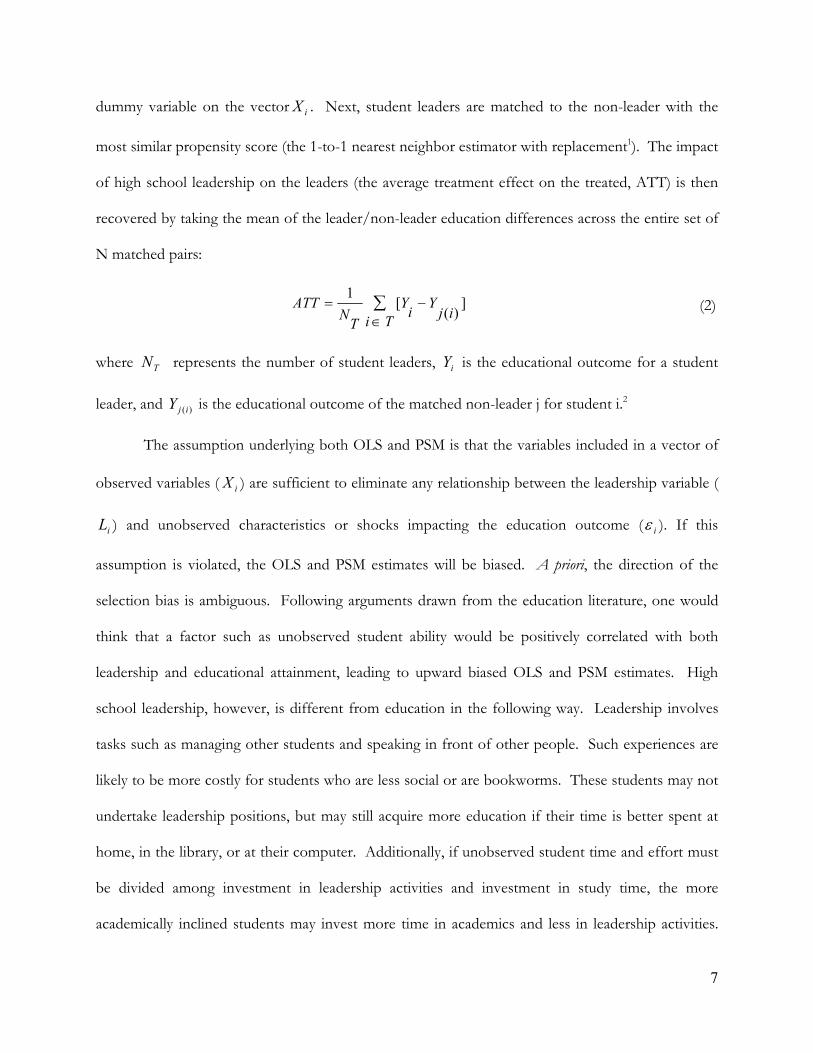
dummy variable on the vector iX . Next, student leaders are matched to the non-leader with the

most similar propensity score (the 1-to-1 nearest neighbor estimator with replacement1). The impact

of high school leadership on the leaders (the average treatment effect on the treated, ATT) is then

recovered by taking the mean of the leader/non-leader education differences across the entire set of

N matched pairs:

])(

[1

ijY

Tii

Y

TN

ATT −

∈

= ∑ (2)

where TN represents the number of student leaders, iY is the educational outcome for a student

leader, and )(ijY is the educational outcome of the matched non-leader j for student i.2

The assumption underlying both OLS and PSM is that the variables included in a vector of

observed variables ( iX ) are sufficient to eliminate any relationship between the leadership variable (

iL ) and unobserved characteristics or shocks impacting the education outcome ( iε ). If this

assumption is violated, the OLS and PSM estimates will be biased. A priori, the direction of the

selection bias is ambiguous. Following arguments drawn from the education literature, one would

think that a factor such as unobserved student ability would be positively correlated with both

leadership and educational attainment, leading to upward biased OLS and PSM estimates. High

school leadership, however, is different from education in the following way. Leadership involves

tasks such as managing other students and speaking in front of other people. Such experiences are

likely to be more costly for students who are less social or are bookworms. These students may not

undertake leadership positions, but may still acquire more education if their time is better spent at

home, in the library, or at their computer. Additionally, if unobserved student time and effort must

be divided among investment in leadership activities and investment in study time, the more

academically inclined students may invest more time in academics and less in leadership activities.

8

In either of these cases, the estimated impact of leadership with OLS or PSM will be understated.

Measurement error in the leadership variable will also bias the OLS and PSM estimates toward zero.

IV estimation is used to control for selection on unobserved characteristics under the

assumption that there is a set of variables ( iZ ) that are related to iL but are uncorrelated with iε .

The NELS dataset includes several students from each high school (21, on average). This attribute

allows for the construction of a school-level measure of leadership opportunities to be used as an

instrument for the individual’s leadership choice.3 This variable is constructed by taking the number

of leaders, excluding the student, divided by all of the individuals in a student’s school. Since school

enrollment is included in all models, this measure should capture differences in leadership

opportunities that are not simply reflective of differences in school size. For additional

identification, dummy indicators of whether the student is the oldest child in his family (and has a

younger sibling) and whether or not he is a twin as well as the interaction of these variables are

included in the first stage equation. The use of the oldest child indicator follows from the

observation that a first born child is more likely to be a leader than an otherwise identical student

who is a second or third born who is used to following the actions of his elder siblings and is more

content serving in a “follower” role. The use of a twin indicator follows from research drawn from

the sociology field that suggests students with siblings are more likely to participate in sports [Wold

and Anderson (1992)]. Since being a twin is exogenous to the student and provides him with a

playmate of the same age, being a twin may be particularly strong predictor of participation and,

subsequently, leadership. Descriptive statistics of these instruments (Table 1) suggest that each of

these variables does, in fact, differ by leadership status in the expected direction. Controls for school

characteristics, family income and family socioeconomic status are included in all of the model

specifications to help mitigate the concerns over the exclusion restrictions. The plausibility of the

exclusion restrictions is also tested statistically with a Sargan-Hansen over-identification test. In

9

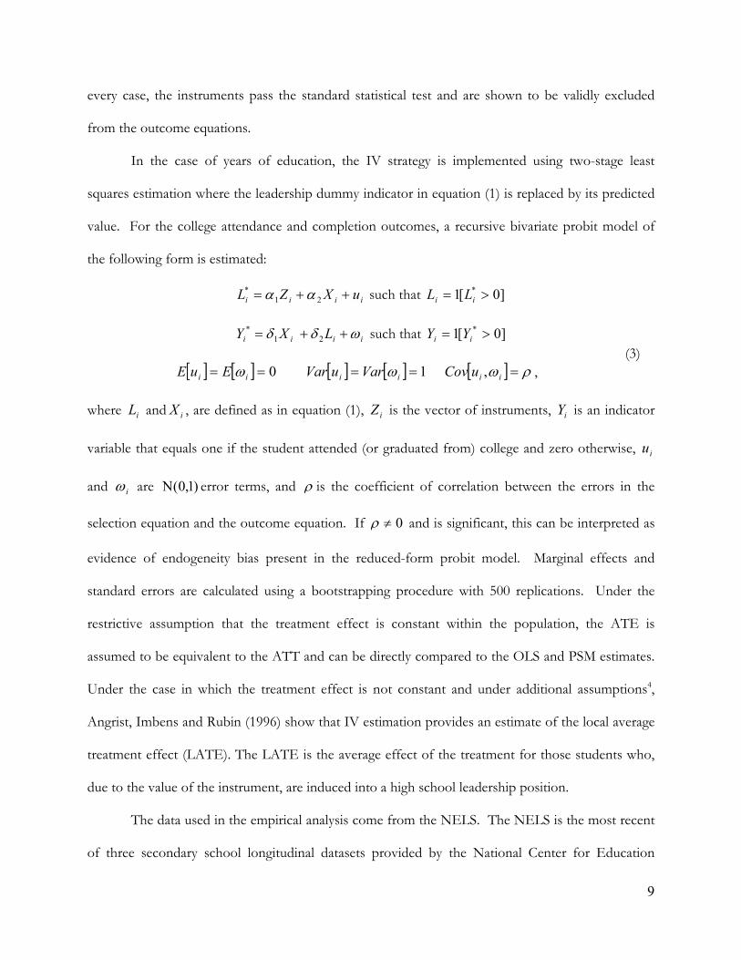
every case, the instruments pass the standard statistical test and are shown to be validly excluded

from the outcome equations.

In the case of years of education, the IV strategy is implemented using two-stage least

squares estimation where the leadership dummy indicator in equation (1) is replaced by its predicted

value. For the college attendance and completion outcomes, a recursive bivariate probit model of

the following form is estimated:

iiii uXZL ++= 21

* αα such that ]0[1 * >= ii LL

iiii LXY ωδδ ++= 21

* such that ]0[1 * >= ii YY

(3)

[ ] [ ] 0== ii EuE ω [ ] [ ] 1== ii VaruVar ω [ ] ρω =iiuCov , ,

where iL and iX , are defined as in equation (1), iZ is the vector of instruments,

iY is an indicator

variable that equals one if the student attended (or graduated from) college and zero otherwise, iu

and iω are )1,0(Ν error terms, and ρ is the coefficient of correlation between the errors in the

selection equation and the outcome equation. If 0≠ρ and is significant, this can be interpreted as

evidence of endogeneity bias present in the reduced-form probit model. Marginal effects and

standard errors are calculated using a bootstrapping procedure with 500 replications. Under the

restrictive assumption that the treatment effect is constant within the population, the ATE is

assumed to be equivalent to the ATT and can be directly compared to the OLS and PSM estimates.

Under the case in which the treatment effect is not constant and under additional assumptions4,

Angrist, Imbens and Rubin (1996) show that IV estimation provides an estimate of the local average

treatment effect (LATE). The LATE is the average effect of the treatment for those students who,

due to the value of the instrument, are induced into a high school leadership position.

The data used in the empirical analysis come from the NELS. The NELS is the most recent

of three secondary school longitudinal datasets provided by the National Center for Education

10

Statistics.5 The survey includes 12,144 individuals who were in eighth grade in 1988 and included in

the fourth follow-up in 2000. The participants were re-interviewed in 1990, 1992, 1994 and 2000.

The students, their parents, their teachers and their school counselors were interviewed. The dataset

contains a rich collection of both individual and school level characteristics. For the purposes of

this research, this study is particularly well-suited as it asks a number of questions covering a wide

range of extracurricular activities. Moreover, the responses include an indicator of whether the

individual was a participant, a non-participant or if he was an officer or a captain in the particular

activity. This allows for the construction of a dummy indicator for high school leadership

experience. An individual is considered to be a high school leader if there is evidence that he held

any leadership position (athletic captain or club officer) in either the tenth or twelfth grade.6

Since the effect of high school leadership is estimated using three different econometric

approaches, a common analysis dataset is constructed so that each method is applied to the same

sample of students. Due to missing leadership, education, control or instrumental variables, this

reduces the original sample of 12,144 students who were included in the fourth follow-up survey to

a sample of 9,670 students. In the analysis sample, 4,180, or 43.2%, of students are leaders, while

5,490 students (56.8%) are non-leaders. Admittedly, 43.2% seems like a high proportion of student

leaders. However, Kuhn and Weinberger (2005) find similar proportions of student leaders in all

three of their datasets. In their Project Talent sample, 57.7% of students are leaders; and, in the

High School Beyond sample that only considers twelfth grade leadership, 48% of the students are

leaders. These high percentages may reflect student reporting error. Alternatively, they may simply

be a result of the comprehensive list of activities that are used to construct the leadership indicators.

In addition, within a given activity, there may be multiple leadership positions. The National Honor

Society, for example, likely has a president, vice president, secretary and a treasurer. Unfortunately,

the data does not allow one to differentiate between a club president and a club treasurer.

11

Three different measures are used to assess the impact of high school leadership on

subsequent educational attainment in the primary analyses: (1) years of education, (2) probability of

attending any post-secondary institution, and (3) probability of holding a college degree. A

supplemental analysis also considers attendance at a four-year school first as the dependent variable.

Each of these outcome variables is measured in the year 2000, approximately eight years after high

school. Table 1 presents descriptive statistics disaggregated by leadership status. A simple

comparison of the means of each measure of educational attainment suggests a positive relationship

between high school leadership and educational attainment. Compared with non-leaders, for

example, leaders have, on average, obtained roughly one more year of education. In addition, over

90% of leaders have acquired some post-secondary education by 2000, while only 76% of non-

leaders have attended. While 50% of high school leaders are college graduates on 26% of non-

leaders have a college degree. Finally, conditional on attendance, a higher proportion of leaders

attended a four-year school first. Each of these differences in means is statistically significant at the

one percent level. Evidence provided by the descriptive statistics suggests that there is also

substantial heterogeneity in many individual, family, and school characteristics across the two

groups. (TABLE 1 ABOUT HERE)

Results

The main results are reported in Table 2. All of the model specifications include controls for

standard demographic characteristics (gender, race, age); family background characteristics (family

income and socioeconomic status); school characteristics (public, Catholic, enrollment, percent of

students with free lunch, percent of Black and Hispanic students, and school average math score);

and regional differences (northeast, midwest, and west). Each model also controls for differences in

endowed or attained cognitive ability by including standardized high school and eighth grade math

test scores. Self-reported measures of popularity, athletic ability and locus of control may be

12

endogenous with respect to high school leadership. However, the inclusion of these additional

characteristics may capture some characteristics that are often “unobserved” (motivation,

confidence, etc.) and help to control for selection bias. Columns (a), (c) and (e) report results from

Model 1, which does not include controls for popularity, athletic ability and locus of control.

Columns (b), (d) and (e) are from Model 2, in which these controls are included. Coefficients on

math scores are also reported in Table 2 to provide a reference of relative magnitude of the

leadership effects.

OLS and probit results (reported in columns (a) and (b) ) are quite similar, suggesting the

OLS results are not highly sensitive to the linearity or common support assumptions. Results from

each model specification are precisely estimated and indicate that, ceteris paribus, leadership is

associated with a 0.35 to 0.44 year increase in education. These estimates are not small. Compared

with the effect of cognitive ability, they are roughly equivalent to a 6.5 to 7 percentile point increase

in math test score.7 These effects are also of similar magnitude to Altonji’s (1995) largest estimates

of an additional year of science, foreign language or math class on total years of education (0.270,

0.590, 0.424, respectively). The results also suggest high school leadership is associated with a higher

probability of both college attendance (5 to 7 percent) and college graduation (9.5 to 14 percent).

These estimates are comparable to math score increases of approximately 5.5 to 8 percentile points.8

(TABLE 2 ABOUT HERE)

Before discussing the instrumental variables estimates, it is important to demonstrate the

validity of the instruments. In each model specification, the p-value on the Cragg-Donald F-statistic

is essentially zero, providing evidence that the instruments are strong predictors of high school

leadership and are therefore sufficiently powerful.9 First stage results (Table 3) also show that both

school leadership opportunities and the interaction between twin and oldest child variables have an

independent statistically significant impact on high school leadership. Table 2 reports p-values from

13

a Sargan-Hansen test of over-identifying restrictions for the education outcome equations. The joint

null hypothesis for this test is that all but one of the instruments are uncorrelated with the error term

and are therefore properly excluded from the outcome equation. The Sargan p-values are 0.8559

and 0.8466. Consequently, the null hypothesis cannot be rejected at conventional confidence levels.

Taken together, this evidence indicates that the instruments are valid. (TABLE 3 ABOUT HERE)

Interestingly, the IV estimates are all larger than their corresponding OLS/probit and PSM

estimates. Compared with the OLS and PSM results, both of which suggest a return to high school

leadership of about a half-year increase in educational attainment, the corresponding IV estimates

are over twice the size, or roughly 0.84 to 0.96 years. The corresponding math test score effects

suggest that leadership is equivalent to a 15 to 16 percentile increase in math test scores. There is

also a large difference in magnitude with respect to the probability of attending and graduating from

a post-secondary institution. Whereas probit and PSM estimates suggest a 5 to 7% impact of

leadership on college attendance, the IV result suggests this magnitude is over 20%. Both IV

estimates of the impact of leadership on college graduation are around 35%, which is also much

larger than their OLS and PSM counterparts (9.5% to 14%). These estimates are also greater than

those reported by Lozano (2008), which imply leadership is associated with an increased probability

of college attendance and graduation of about 7% and 28%, respectively.

Lozano (2008) finds that leadership is predicted to have an even higher impact on the

probability of attending a four-year school (31% to 40%). Findings from a supplemental analysis

that examines the impact of high school leadership on the probability of attending a four-year school

first (Table 4) support this finding. The analysis is limited to students who attended any post-

secondary school, which reduces the original sample from 9,970 to 7,910 students. The results of

these analyses are similar to the main results of the paper, suggesting leadership also has a large,

positive causal impact on the likelihood of attending a four-year (versus two-year) school. This

14

finding is important given the well-documented negative effects of two-year college attendance on

bachelor’s degree completion [Alfonso (2006), Miller (2007), Long and Kurlaender (2008), Doyle

(2009), Reynolds (2009)]. (TABLE 4 ABOUT HERE)

Discussion and Robustness Checks

The finding that the IV estimates are much larger than their OLS and PSM counterparts may

seem counter-intuitive. If the source of unobserved heterogeneity is the traditional ‘ability’ bias,

then IV estimation which correctly controls for such bias should result in estimates that are of

smaller magnitude than their corresponding OLS or PSM estimates. Here the results reflect the

opposite. However, while the theoretical literature on the return on education frequently suggests

that OLS results will be biased in the upward direction, empirical researchers who rely on supply

side features of the education system often find IV estimates that are at least as large as or larger

than their corresponding OLS estimates.10 In this sense, the results reported in this paper are

consistent with much of the empirical literature on education.

The most straightforward explanation is that, rather than being upward biased, the OLS and

PSM estimates are actually biased downward. The high proportion of student leaders in the sample

may be suggestive of student reporting error, biasing the OLS and PSM estimates towards zero. As

discussed earlier, this result could also reflect selection bias due to an unobserved characteristic, such

as being a bookworm, that makes a student less likely to be a leader but more likely to attain further

education. In either case, the instrumental variables estimation procedure is appropriately correcting

for the negative bias. Results from the bivariate probit models suggest that this explanation is likely.

In both model specifications for both discrete outcomes, the correlation coefficient is large, negative

and statistically significant, indicating that OLS and PSM estimates are biased downward. In other

words, the OLS and PSM likely understate the true impact of leadership.

15

Card (2001) puts forth an alternative interpretation for similar results found in the returns to

schooling literature. If the impact of leadership is not constant across the student population, then

the LATE, the estimated effect with IV, may differ from the ATT or ATE. Card (2001) suggests

that instrumental variables estimates may be larger than OLS estimates because the IV method is

measuring a treatment effect for a small low-education group with a higher marginal return to

education, causing the LATE to be greater than the ATE or ATT. Here the IV estimates could be

larger because the students who are induced into a leadership position due to the instruments have a

greater marginal return to their leadership experience than the students who chose to be leaders.

Consider school leadership activities, where an increase indicates a greater availability of school

activities. Following Card’s argument, if the students with initially higher marginal costs of high

school leadership (those who will be more affected by the cost reduction imposed by greater

availability of activities) also have a greater marginal return to leadership, then the IV estimates will

overstate the average impact of high school leadership.

Another possible explanation for these results is that, despite passing the standard statistical

tests, the instruments used in the analysis are simply not valid. To further test the instrument

validity, Table 5 presents IV results from alternative specifications that rely on different sets of

identifying assumptions. Results from these analyses indicate that the IV results are not particularly

sensitive to the choice of model specification. For instance, even in models that do not rely on

school leadership opportunities for identification (column D), the IV estimates are much larger than

their corresponding OLS or PSM counterparts. This result helps ease one potential concern that the

large IV estimates are being driven by the school leadership opportunities instrument which, if

positively correlated with unobserved school quality, would lead to upward biased IV estimates.

Another concern is that the twin/oldest child indicators should not be excluded from the outcome

equations. Table 6 further investigates this concern by directly entering each instrument into the

16

outcome equation. In each and every case, not one of the coefficients on the instrumental variable

is statistically different from zero. This result provides further evidence that the instruments are

appropriately excluded from the outcome equation. (TABLES 5 & 6 ABOUT HERE)

Regardless of the interpretation of these results, every estimation method and model

specification examined suggests the impact of high school leadership is large, positive, and

significant in an economic and a statistical sense. The smallest estimates found are non-trivial and

the evidence implies the impact may be much larger for some students. These results suggest OLS

estimates of the correlation between leaders and later outcomes such as those reported by Kuhn and

Weinberger (2005) and Lozano (2008) may understate the true impact of leadership experiences.

Conclusion

This paper contributes to the literature by providing new evidence that indicates high school

leadership does, in fact, have a large positive impact on the future educational attainment of the

average student. Rather than providing specific estimates that can be relied upon for policy

recommendations, this paper illustrates that even the smallest estimated effects are non-trivial and

provides evidence that suggests the true causal impact for the group of students less likely to actively

seek out leadership positions may be much larger. Since the availability of leadership positions

depends upon the existence of school activities that provide such leadership opportunities, the

evidence presented in this paper indicates that decisions regarding financial cutbacks for

extracurricular activities should not be taken lightly. While the paper cannot explicitly address the

implications of extracurricular cutbacks or programs such as play-to-play, the results suggest that

such actions could be quite detrimental for those students who are stripped of the opportunity to

undertake a leadership position. These results motivate further research on this topic. Studies which

are able to quantify the impact of extracurricular funding cutbacks or programs such as pay-to-play

would be particularly useful.

17

Table 1. Descriptive Statistics

Mean Std. Dev Mean Std. Dev.

Outcomes:

Years of education 14.968 1.540 13.994 1.687 0.974 ***

Any post-secondary education 0.911 0.285 0.763 0.425 0.148 ***

College graduate 0.514 0.500 0.262 0.440 0.253 ***

Four year first, conditional on attendance 0.688 0.008 0.456 0.008 0.233 ***

Controls:

Male 0.468 0.499 0.478 0.500 -0.011

Black 0.088 0.284 0.089 0.285 -0.001

Hispanic 0.094 0.292 0.137 0.344 -0.043 ***

Age (years) 25.800 0.505 25.877 0.564 -0.077 ***

8th grade socioeconomic status indice 0.147 0.754 -0.182 0.759 0.329 ***

High school socioeconomic status indice 0.209 0.773 -0.129 0.776 0.338 ***

8th grade family income indice 10.378 2.364 9.504 2.579 0.874 ***

High school family income indice 10.674 2.413 9.880 2.575 0.794 ***

High school enrollment 234.769 173.726 292.595 182.456 -57.826 ***

% free lunch in high school 19.067 20.300 21.205 21.168 -2.138 ***

% Black in high school 9.084 19.122 11.323 21.196 -2.239 ***

% Hispanic in high School 9.955 18.684 10.782 19.028 -0.827 **

Public high school 0.792 0.406 0.859 0.348 -0.067 ***

Catholic high school 0.073 0.259 0.059 0.236 0.013 ***

Private (non-Catholic) high school 0.135 0.342 0.081 0.273 0.054 ***

Mean school-level high school math score 5.214 0.575 5.084 0.536 0.130 ***

High school math score percentile 5.443 0.965 4.966 0.969 0.477 ***

8th grade math score percentile 5.480 1.029 5.009 0.964 0.472 ***

8th grade: athletic 0.340 0.474 0.195 0.397 0.145 ***

High school: athletic 0.226 0.418 0.094 0.292 0.131 ***

8th grade: popular 0.201 0.401 0.127 0.333 0.074 ***

High school: popular 0.185 0.388 0.085 0.279 0.099 ***

8th grade: locus of control 0.173 0.674 -0.015 0.699 0.188 ***

High school: locus of control 0.184 0.750 -0.026 0.740 0.210 ***

Northeast 0.191 0.393 0.190 0.393 0.001

Midwest 0.287 0.452 0.276 0.447 0.010

West 0.180 0.384 0.207 0.405 -0.026 ***

South 0.341 0.474 0.325 0.469 0.015

Instruments:

% HS peers in leadership positions 0.400 0.170 0.356 0.156 0.043 ***Twin 0.046 0.210 0.037 0.189 0.009 **Oldest Child 0.338 0.473 0.304 0.460 0.034 ***Twin*Oldest child 0.014 0.118 0.007 0.086 0.007 ***

Notes:

a. Difference is calculated as mean(leaders) - mean(non-leaders). *,**, and *** denote statistical

significance at the 10%, 5%, and 1% levels, respectively.

b. Per NCES restricted-data use agreements, samples sizes have been rounded to nearest 10.

Differencea

N= 4,180 N= 5,490

Leaders Non-Leaders

18

Table 2. The Impact of High School Leadership on Subsequent Educational Attainment

A. Years of Education

High School Leadership 0.446 *** 0.400 *** 0.346 *** 0.391 *** 0.963 * 0.835 *

(0.028) (0.028) (0.038) (0.046) (0.528) (0.510)

High School Math Score 0.624 *** 0.590 *** 0.586 *** 0.559 ***

(0.028) (0.028) (0.049) (0.047)

R-squared 0.411 0.420

F-statistic 7.62 8.08

(p-value) 0.0000 0.000

Sargan Statistic (p-value) 0.8559 0.8466

B. Any Post-Secondary

Educationb

High School Leadership 0.070 *** 0.064 *** 0.050 *** 0.059 *** 0.243 *** 0.213 ***

(0.006) (0.007) (0.011) (0.009) (0.074) (0.044)

High School Math Score 0.080 *** 0.076 ***

(0.006) (0.006)

R-squared 0.261 0.268

Rho -0.503 *** -0.396 ***

(0.157) (0.184)

College Graduateb

High School Leadership 0.143 *** 0.125 *** 0.095 *** 0.104 *** 0.341 *** 0.357 ***

(0.011) (0.012) (0.015) (0.015) (0.116) (0.115)

High School Math Score 0.229 *** 0.219 ***

(0.011) (0.011)

R-squared 0.320 0.329

Rho -0.490 *** -0.568 ***

(0.063) (0.089)

Popular, Athletic, Locus of

Control No Yes No Yes

N=9,670 individuals

Notes:

a. Robust standard errors clustered at the school level are reported in parenthesis. *,**, and ***

denote statistical significance at the 10%, 5%, and 1% level, respectively. All specifications

include controls for demographics, family background, region, school quality, and cognitive ability (math scores).

b. Reported coefficients in columns (a) and (b) on Any Post-Secondary and College Graduate are marginal

effects from probit models.

c. Instruments include twin, oldest child, twin*oldest child and school leadership opportunities.

d. Per NCES restricted-data use agreements, samples sizes have been rounded to nearest 10.

No Yes

OLS & Probit Propensity Score Matching Instrumental Variablesc

(a) (b) (c) (d) (e) (f)

19

Table 3. First Stage Results

School Leadership Opportunities 0.134 *** 0.122 ***

(0.041) (0.040)

Oldest Child*Twin 0.119 ** 0.113 **

(0.054) (0.053)

Twin 0.040 0.048 *

(0.029) (0.028)

Oldest Child 0.009 0.016

(0.010) (0.010)

Popular, Athletic, Locus of Control

F-statistic

P-value

Sargan P-Value on over-id test

Notes:

a. *,**,*** denotes statistical significance at the 10, 5, and 1% level, respectively.

b. All specifications include controls for demographic, family, region, school, and cognitive ability

(math scores).

0.8559 0.8466

No Yes

7.62 8.08

0.0000 0.0000

Table 4. High School Leadership and College Attendance, Four-Year School First

High School Leadership 0.156 *** 0.141 *** 0.114 *** 0.103 *** 0.378 *** 0.362 ***

(0.012) (0.013) (0.016) (0.017) (0.115) (0.136)

High School Math Score 0.197 *** 0.191 ***

(0.013) (0.013)

R-squared 0.239 0.244

Rho -0.599 *** -0.534 **

(0.123) (0.142)

Number of observations

Popular, Athletic, Locus of

ControlNotes:

a. Robust standard errors are reported in parenthesis. *,**, and *** denote statistical significance at the 10%, 5%, and 1% level, respectively.

All specifications include controls for demographics, family background, region, school quality, and cognitive ability (math scores).

b. Reported coefficients are marginal effects.

c. Instruments include twin, oldest child, twin*oldest child and school leadership opportunities.

d. Per NCES restricted-data use agreements, sample sizes have been rounded to nearest 10.

Probit Propensity Score Matching Bivariate Probit

(a) (b) (c) (d) (e) (f)

7,910 7,910

No YesNo Yes No

7,910 7,910 7,910 7,910

Yes

20

Table 5. Alternative Instrumental Variables Specifications

Education

High School Leadership 0.835 * 1.024 * 1.160 0.895

(0.502) (0.569) (0.786) (0.762)

F-statistic 8.08 13.72 13.77 14.11

F-stastic p-value 0.0000 0.0000 0.0000 0.000

Sargan p-value 0.8466 0.8154 n/a n/a

Any Post-Secondary Education

High School Leadership 0.213 *** 0.219 *** 0.216 *** 0.198 ***

(0.044) (0.067) (0.040) (0.063)

Rho -0.396 -0.417 -0.480 -0.426

(0.184) (0.175) (0.137) (0.170)

College Graduate

High School Leadership 0.357 *** 0.365 *** 0.375 *** 0.373 ***

(0.115) (0.079) (0.073) (0.075)

Rho -0.568 -0.583 -0.603 -0.599

(0.089) (0.084) (0.078) (0.080)

Instruments:

School Leadership Opportunities X X X

Twin X

Eldest Child X

Twin*Eldest Child X X X

N=9,670 individualsNote:

a. Robust standard errors are reported in parenthesis. *,**, and *** denote statistical significance at the 10%, 5%, and

1% level, respectively. All specifications include controls for demographics, family background, region, school quality, and

cognitive ability (math scores).

b. Reported coefficients on Any Post-Secondary and College Graduate are marginal effects from probit models.

c. Per NCES restricted-data use agreements, sample sizes have been rounded to nearest 10.

(a) (b) (c) (d)

21

Table 6. Instrumental Variables Exclusion Restrictions

Model 2

(a) (b)

Outcome: Years of Education

Twin -0.050 -0.048

(0.082) (0.083)

[z=0.61] [z=-.057]

Oldest Child -0.014 -0.051

(0.030) (0.031)

[z=-0.46] [z=-.051]

Twin*Oldest Child 0.012 0.018

(0.173) (0.175)

[z=0.07] [z=-.10]

School Leadership Opportunities 0.059 0.070

(0.138) (0.125)

[z=0.43] [z=0.56]

Popular, Athletic, Locus of Control No Yes

N= 9,670

Notes:

a. Both model specifications include controls for demographics, family background, region, school quality,

and cognitive ability (math scores). Robust standard errors are reported in parenthesis.

b. Coefficients represent estimates of the given variable on total years of education from separate

regressions where leadership is instrumented with the other three instruments.

c. Per NCES restricted-data use agreements, sample sizes have been rounded to nearest 10.

Model 1

22

References Alfonso, Mariana. 2006. “The impact of community college attendance on baccalaureate attainment.” Research in Higher Education 47(8): 873-903. Altonji, J.G. 1995. “The effects of high school curriculum on education and labor market outcomes.” Journal of Human Resources 30(3): 409-438. Anderson, D.J. 2001. “If you let me play: The effects of participation in high school athletics on students’ educational and labor market success.” The University of New Mexico, working paper. Angrist. J.D., G.W. Imbens and D.B. Rubin. 1996. “Identification of Causal Effects Using Instrumental Variables.” Journal of the American Statistical Association 91: 444-455. Barron, J.M., B.T. Ewing, and G.R. Waddell. 2000. The effects of high school athletic participation on education and labor market outcomes. Review of Economics and Statistics 82(3): 409-421. Becker, G. Human Capital. New York: National Bureau of Economic Research; 1964. Brady, E and R. Glier. 2004. “To play sports, many U.S. students must pay.” USA Today. July 29. <http://www.usatoday.com/sports/preps/2004-07-29-pay-to-play_x.htm> Brown, Justin. 2002. “Will pay-to-play ruin schools sports?” The Christian Science Monitor. September 20. <http://www.csmonitor.com/2002/0920/p12s01-alsp.html> Card, D. 2001. “Estimating the return to schooling: Progress on some persistent econometric problems.” Econometrica 69(5): 1127-1160. Dehijia, R. and S. Wahba. 1999. “Causal effects in non-experimental studies: Reevaluating the evaluation of training programs”. Journal of the American Statistical Association 94(448): 1053-1062. Dehijia, R. and S. Wahba. 2002. “Propensity score matching methods for nonexperimental causal studies.” Review of Economics and Statistics 84(1): 151-161. Diaz, J.J. and S. Handa. 2006. “As assessment of propensity score matching as a nonexperimental impact estimator. Evidence from Mexico’s PROGRESA program.” Journal of Human Resources 41(2): 319-345. Doyle, W.R. 2009. “The effect of community college enrollment on bachelor’s degree completion.” Economics of Education Review 28(2): 199-206. Eide, E.R. and N. Ronan. 2001. “Is participation in high school athletics an investment or a consumption good? Evidence from high school and beyond.” Economics of Education Review 20: 431-442. Ewing, B.T. 1995. “High school athletics and the wages of black males.” Review of Black Political Economy 65-78.

23

Ewing, B.T. 2007. “The labor market effects of high school athletic participation: Evidence from Wage and Fringe Benefit Differentials.” Journal of Sports Economics 8(3): 255-265. Fahey, Rich. 2007. “More high school athletes have to pay to play.” The Boston Globe, September 2. <http://www.boston.com/news/local/articles/2007/09/02/more_high_school_athletes_have_to_pay_to_play/> Heckman, J., H. Ichimura and P. Todd. 1998. “Matching as an econometric evaluation estimator.” Review of Economic Studies 65(2): 261-294. Heckman, J., H. Ichimura and P. Todd. 1997. “Matching as an econometric evaluation estimator: Evidence from evaluating a job training program.” Review of Economic Studies 64(4): 605-654. Kuhn, P. and C. Weinberger. 2005. “Leadership skills and wages.” Journal of Labor Economics 23(3): 395-436. Leeds, M. 2003. “Race, Opportunities, and Incentives: The Importance of Timing.” Review of Black Political Economy 30(3): 55-69. Leeds, M. A., C. Miller and J. Stull. 2007. “Interscholastic Athletics and Investment in Human Capital.” Social Science Quarterly 88(3): 729-741. Lipscomb, S. 2006. “Secondary school extracurricular involvement and academic achievement: a fixed effects approach.” Economics of Education Review 26: 463-472. Long, B.T. and M. Kurlaender. 2008. “Do community colleges provide a viable pathway to a Baccalaureate Degree?” NBER Working Papers, 14367. Lozano, F.A. 2008. “Language, high school leadership and the postsecondary outcomes of Hispanic students.” Economics of Education Review 27: 342-353. Miller, D. W. 2007. “Isolating the causal impact of community college enrollment on educational attainment and labor market outcomes in Texas. SIEPR Discussion Paper 06-33. Popke, Michael. 2009. “Elimination game: As districts slash expenses, some athletic directors find themselves in either the classroom or the unemployment line.” Athletic Business, April. http://athleticbusiness.com/articles/article.aspx?articleid=2044&zoneid=36 Rosenbaum, P.R. and D.B. Rubin. 1983. “The central role of the propensity score in observational studies for causal effects.” Biometrica 70: 41-55. Author. 2009. “High school leadership, educational attainment and post-schooling earnings.” Siebert, J.W., G.C. Davis, K.K. Litzenberg, and J.M. Broder. 2002. “Time allocation decisions associated with job market preparation: Undergraduate perceptions versus market realities.” American Journal of Agricultural Economics 84(1): 222-233.

24

Smith, J.A. and P.E. Todd. 2005. “Does matching overcome LaLonde’s critique of non-experimental estimators?” Journal of Econometrics 125(1-2): 305-353. Spence, M. 1973. “Job market signaling.” Quarterly Journal of Economics 87: 355-374. Staples, A. 2009. “The impact of an Ohio School district’s decision to cut sports.” <http://sportsillustrated.cnn.com/2009/writers/andy_staples/09/16/nosports/index.html., September 17. Stern, Sam. 2010. “In New Providence, pay-to-play sports carries high price yag.” <http://www.nj.com/independentpress/index.ssf/2010/10/in_new_providence_pay-to-play.html> October 21. Stevenson, B. 2006. “Beyond the classroom: Using Title IX to measure the returns to high school Sports.” Federal Reserve Bank of San Francisco Working Paper Series, Working Paper 2006-44. Stock, J.H., J. Wright and M. Yogo. 2002. “A survey of weak instruments and weak identification in generalized method of moments.” Journal of Business & Economic Studies 20(4): 518-529. Stock, J.H. and M. Yogo. 2005. “Testing for weak instruments in linear IV regression.” In D.W.K. Andrews and J.H. Stocks (eds), Identification and Inference for Econometric Models: Essays in Honor of Thomas Rothenberg. Cambridge, UK: Cambridge University Press. Stone, Elizabeth. 2010. “Leadership and college admissions.” Examiner.com, August 28, 2010.<http://www.examiner.com/college-admissions-in-san-francisco/leadership-and-college-admissions> Tomsho, Robert. 2009. “Adding personality to the college admission mix.” The Wall Street Journal, August 19, 2009. <http://online.wsj.com/article/SB10001424052970203612504574342732853413584.html> Wold, B. and N. Anderson. 1992. “Health promotion aspects of family and peer influences on sports participation.” International Journal of Sport Psychology 23: 343-359.

25

Notes

1 Models were also estimated using alternative matching methods. Results are not highly sensitive to

the choice of matching approach.

2 Since the estimates rely on estimated propensity scores, the standard errors are estimated using the

bootstrap method with 50 replications.

3 Anderson (2001) and Altonji (1995) both rely on a similar instrument.

4 These are (1) stable unit treatment values, (2) random assignment to treatment, (3) valid exclusion

restriction, (4) nonzero causal effect of the IV on treatment status and (5) monotonicity.

5 In contrast to the NLS-72 and HS&B, Title IX was fully implemented by the time students of the

NELS were in high school. Thus, in addition to it being the most current survey, use of the NELS

avoids the problem of confounding the influence of expanding and uneven athletic opportunities for

women. Interestingly, however, point estimates (AUTHOR, 2009) using the HS&B are nearly

identical to those reported in this article.

6 A full list of activities used to create leadership measure is available upon request.

7 This is calculated by taking the coefficient on leadership divided by the coefficient on math score

(which represents the effect of a 10 percentile increase in math score) multiplied by 10.

8 OLS results change little when high school fixed effects are included in the models.

9 While the F-statistics do not meet the commonly cited threshold of 10 (reflecting less than 10%

bias), the F-statistics do exceed the threshold for 20 percent bias (critical value = 6.71) as given by

Stock and Yogo (2005). The estimates are also robust to limited-information maximum likelihood

estimation, which Stock, Wright and Yogo (2002) argue is more robust to weak instruments than

2SLS (results available on request).

10 Card (2001) summarizes results from 11 studies that find IV estimates that are larger than OLS

estimates.