The Impact of Health Care Reform on Hospital and

Preventive Care: Evidence from MassachusettsI

Jonathan T. Kolstada, Amanda E. Kowalskib,∗

aThe Wharton School, University of Pennsylvania and NBERbDepartment of Economics, Yale University and NBER

Abstract

In April 2006, Massachusetts passed legislation aimed at achieving near-universal health insurance coverage. The key features of this legislation werea model for national health reform, passed in March 2010. The reform givesus a novel opportunity to examine the impact of expansion to near-universalcoverage state-wide. Among hospital discharges in Massachusetts, we findthat the reform decreased uninsurance by 36% relative to its initial leveland to other states. Reform affected utilization by decreasing length of stay,the number of inpatient admissions originating from the emergency room,and preventable admissions. At the same time, hospital cost growth did notincrease.

Keywords: health, health care, health reform, insurance, hospitals,Massachusetts, preventive care

1. Introduction

In April 2006, the state of Massachusetts passed legislation aimed atachieving near-universal health insurance coverage. This legislation has beenconsidered by many to be a model for the national health reform legislationpassed in March 2010. In light of both reforms, it is of great policy impor-tance to understand the impact of a growth in coverage to near-universal

∗Corresponding author. Mailing address: Department of Economics, YaleUniversity, Box 208264, New Haven, CT 06520-8264, United States. E-mail:amanda.kowalski@yale.edu. Telephone: +1-202-670-7631. Fax: +1-203-432-6323.

Email addresses: jkolstad@wharton.upenn.edu (Jonathan T. Kolstad),amanda.kowalski@yale.edu (Amanda E. Kowalski)

Preprint submitted to Journal of Public Economics May 24, 2012

levels, unprecedented in the United States. In theory, insurance coveragecould increase or decrease the intensity and cost of health care, dependingon the underlying demand for care and its impact on health care delivery.Which effect dominates in practice is an empirical question.

Although previous researchers have studied the impact of expansions inhealth insurance coverage, these studies have focused on specific subpopu-lations – the indigent, children, and the elderly (see e.g.Currie and Gruber(1996); Finkelstein (2007); Card et al. (2008); Finkelstein et al. (2012)). TheMassachusetts reform gives us a novel opportunity to examine the impact ofa policy that achieved near-universal health insurance coverage among theentire state population. Furthermore, the magnitude of the expansion in cov-erage after the Massachusetts reform is similar to the predicted magnitude ofthe coverage expansion in the national reform. In this paper, we are the firstto use hospital data to examine the impact of this legislation on insurancecoverage, patient outcomes, and utilization patterns in Massachusetts. Weuse a difference-in-differences strategy that compares Massachusetts after thereform to Massachusetts before the reform and to other states.

The first question we address is whether the Massachusetts reform re-sulted in reductions in uninsurance. We consider overall changes in coverageas well as changes in the composition of types of coverage among the entirestate population and the population who were hospitalized. One potentialimpact of expansions in publicly subsidized coverage is to crowd-out privateinsurance (Cutler and Gruber (1996)). The impact of the reform on the com-position of coverage allows us to consider crowd-out in the population as awhole as well as among those in the inpatient setting.

After estimating changes in the presence and composition of coverage,we turn to the impact of the reform on hospital and preventive care. Wefirst study the intensity of care provided. Because health insurance low-ers the price of health care services to consumers, a large-scale expansionin coverage has the potential to increase demand for health care services,the intensity of treatment, and cost. Potentially magnifying this effect aregeneral equilibrium shifts in the way care is supplied due to the large mag-nitude of the expansion (Finkelstein (2007)). Countervailing this effect isthe monopsonistic role of insurance plans in setting prices and quantities forhospital services. To the extent that health reform altered the negotiatingposition of insurers vis a vis hospitals, expansions in coverage could actuallyreduce supply of services, intensity of treatment, or costs. Furthermore, theexistence of insurance itself can also alter the provision of care in the hospital

2

directly (e.g. substitution towards services that are reimbursed). Withoutcoverage, patients could face barriers to receiving follow up treatment (typi-cally dispensed in an outpatient setting or as drug prescriptions); potentiallyreducing the efficacy of the inpatient care they receive or altering the lengthof time they stay in the hospital. Achieving near-universal insurance couldalter length of stay and other measures of services intensity though physicallimits on the number of beds in the hospital, efforts to increase through-put in response to changes in profitability, or changes in care provided whenphysicians face a pool of patients with more homogeneous coverage (Gliedand Zivin (2002)). Given these competing hypotheses, expanded insurancecoverage could raise or lower the intensity of care provided.

In addition to changes in the production process within a hospital, weare interested in the impact of insurance coverage on how patients enter thehealth care system and access preventive care. We first examine changes inthe use of the emergency room (ER) as a point of entry for inpatient care.Because hospitals must provide at least some care, regardless of insurancestatus, the ER is a potentially important point of access to hospital care forthe uninsured.1 When the ER is the primary point of entry into the hospital,changes in admissions from the ER can impact welfare for a variety of reasons.First, the cost of treating patients in the ER is likely higher than the cost oftreating the same patient in another setting. Second, the emergency room isdesigned to treat acute health events. If the ER is a patient’s primary pointof care, then he might not receive preventive care that could mitigate futuresevere and costly health events. To the extent that uninsurance led people touse the ER as a point of entry for treatment that they otherwise would havesought through another channel, we expect to see a decline in the number ofinpatient admissions originating in the ER.

We also study the impact of insurance on access to care outside of theinpatient setting. Using a methodology developed by the Agency for Health-care Research and Quality (AHRQ), we are able to study preventive care inan outpatient setting using inpatient data. We identify inpatient admissionsthat should not occur in the presence of sufficient preventive care. If thereform facilitated increased preventive care, then we expect a reduction in

1Under the Emergency Medical Treatment and Labor Act (EMTALA), hospitals mustprovide stabilizing care and examination to people who arrive in the ER for an emergencycondition without considering whether a person is insured or their ability to pay.

3

the number of inpatient admissions meeting these criteria. These measuresalso indirectly measure health in the form of averted hospitalizations. Weaugment this analysis with data on direct measures of access to and use ofoutpatient and preventive care.

Finally, we turn to the impact of the reform on the cost of hospitalcare. We examine hospital-level measures of operating costs (e.g. overhead,salaries, and equipment) that include both fixed and variable costs. Thisallows us to jointly measure the direct effect of insurance on cost – the rela-tive effect of changing the out of pocket price – as well as the potential forquality competition at the hospital level. In the latter case, hospitals fac-ing consumers who are relatively less price elastic (or more quality elastic)increase use of costly services and may also increase use of variable inputsas well as investments in large capital projects in order to attract price-insensitive customers (Dranove and Satterthwaite (1992)). In the extreme,large expansions in coverage might lead to a so called “medical arms race,”in which hospitals make investments in large capital projects to attract cus-tomers and are subsequently able to increase demand to cover these fixedcosts (Robinson and Luft (1987)). The impact of all of these effects wouldbe increased hospital costs as coverage approaches near-universal levels.

Our analysis relies on three main data sets. To examine the impact oncoverage in Massachusetts as a whole, we analyze data from the CurrentPopulation Survey (CPS). To examine coverage among the hospitalized pop-ulation, health care utilization, and preventive care, we analyze the universeof hospital discharges from a nationally-representative sample of approxi-mately 20 percent of hospitals in the United States from the Healthcare Costand Utilization Project (HCUP) National Inpatient Sample (NIS). In addi-tion, we use the Behavioral Risk Factor Surveillance System (BRFSS) datato augment our study of access and preventive care.

We find a variety of results pointing to an impact of the Massachusettsreform on insurance coverage, hospital, and preventive care. First, we finda significant reduction in uninsurance both in the general population andamong those who are hospitalized. In the population as a whole, we findthat uninsurance declined by roughly 6 percentage points, or by about 50%of its initial level. This decline primarily came through increased coverage byemployer-sponsored health insurance (ESHI), which accounted for nearly halfthe change, and secondarily through Medicaid and newly subsidized cover-age available through the Massachusetts connector. Turning to hospital andpreventive care, we find that length of stay in the hospital fell significantly,

4

particularly for long hospital stays. We also find a significant reduction emer-gency room utilization that resulted in an inpatient admission. Admissionsoriginating in the ER declined by 5.2%. The impact on ER utilization waslargest in poorer geographic areas. Our results provide some mixed evidencefor a decline in preventable admissions to the hospital. Without includ-ing covariates that capture patient severity, we find limited evidence that thereform reduced preventable admissions. However, in a specification that con-trols for patient severity, we find clear evidence that preventable admissionswere reduced. Finally, we find little evidence that the Massachusetts reformaffected hospital cost growth. Massachusetts hospital costs appear to havebeen growing faster than the remainder of the country prior to reform andto have continued on the same trajectory.

In the next section, we describe the elements of the reform and its imple-mentation, as well as the limited existing research on its impact. In the thirdsection, we describe the data. In the fourth section, we present the difference-in-differences results for the impact of the reform on insurance coverage andhospital and preventive care. In the fifth section, we discuss the implicationsof our findings for national reform. In the sixth section, we conclude anddiscuss our continuing work in this area.

2. Description of the Reform

The recent Massachusetts health insurance legislation, Chapter 58, in-cluded several features, the most salient of which was a mandate for individ-uals to obtain health insurance coverage or pay a tax penalty. All individualswere required to obtain coverage, with the exception of individuals with reli-gious objections and individuals whose incomes were too high to qualify forstate health insurance subsidies but too low for health insurance to be “af-fordable,” as determined by the Massachusetts Health Insurance ConnectorAuthority. For a broad summary of the reform, see McDonough et al. (2006);for details on the implementation of the reform see The Massachusetts HealthInsurance Connector Authority (2008).

The reform also extended free and subsidized health insurance to low in-come populations in two forms: expansions in the existing Medicaid program(called “MassHealth” in Massachusetts), and the launch of a new programcalled CommCare. First, as part of the Medicaid expansion, the reform ex-panded Medicaid eligibility for children to 300 percent of poverty, and itrestored benefits to special populations who had lost coverage during the

5

2002-2003 fiscal crisis, such as the long-term unemployed. The reform alsofacilitated outreach efforts to Medicaid-eligible individuals and families. Im-plementation of the reform was staggered, and Medicaid changes were amongthe first to take effect. According to one source, “Because enrollment capswere removed from one Medicaid program and income eligibility was raisedfor two others, tens of thousands of the uninsured were newly enrolled justten weeks after the law was signed” (Kingsdale (2009), page w591).

Second, the reform extended free and subsidized coverage through a newprogram called CommCare. CommCare offered free coverage to individualsup to 150 percent of poverty and three tiers of subsidized coverage up to300 percent of poverty. CommCare plans were sold through a new, state-runhealth insurance exchange.

In addition, the reform created a new online health insurance market-place called the Connector, where individuals who did not qualify for free orsubsidized coverage could purchase health insurance coverage. UnsubsidizedCommChoice plans available through the Connector from several health in-surers offered three regulated levels of coverage – bronze, silver, and gold.Young Adult plans with fewer benefits were also made available to individ-uals age 26 and younger. Individuals were also free to continue purchasinghealth insurance through their employers or to purchase health insurancedirectly from insurers.

The reform also implemented changes in the broader health insurancemarket. It merged the individual and small group health insurance markets.Existing community rating regulations, which required premiums to be setregardless of certain beneficiary characteristics of age and gender, remainedin place, though it gave new authority to insurers to price policies based onsmoking status. It also required all family plans to cover young adults for atleast two years beyond loss of dependent status, up to age 26.

Another important aspect of the reform was an employer mandate thatrequired employers with more than 10 full time employees to offer healthinsurance to employees and contribute a certain amount to premiums or paya penalty. The legislation allowed employers to designate the Connector asits “employer-group health benefit plan” for the purposes of federal law.

The financing for the reform came from a number of different sources.Some funding for the subsidies was financed by the dissolution of existing

6

state uncompensated care pools.2 Addressing costs associated with the re-form remains an important policy issue.

The national health reform legislation passed in March 2010 shares manyfeatures of the Massachusetts reform, including an individual mandate to ob-tain health insurance coverage, new requirements for employers, expansionsin subsidized care, state-level health insurance marketplaces modeled on theMassachusetts Connector, and new requirements for insurers to cover depen-dents to age 26, to name a few. For a summary of the national legislation, seeKaiser Family Foundation (2010). Taken together, the main characteristicsof the reform bear strong similarity to those in the Massachusetts reform, andthe impact of the Massachusetts reform should offer insight into the likelyimpact of the national reform.

As Chapter 58 was enacted recently, there has been relatively little re-search on its impact to date. Long (2008) presents results on the preliminaryimpact of the reform from surveys administered in 2006 and 2007. Yelowitzand Cannon (2010) examine the impact of the reform on coverage using datafrom the March 2006-2009 Supplements to the Current Population Survey(CPS). They also examine changes in self-reported health status in an effortto capture the effect of the reform on health. Using this measure of health,they find little evidence of health effects. The NIS discharge data allow usto examine utilization and health effects in much greater detail. Long et al.(2009) perform an earlier analysis using one fewer year of the same data.Long et al. (2009) and Yelowitz and Cannon (2010) find a decline in unin-surance among the population age 18 to 64 of 6.6 and 6.7 percentage points,respectively. We also rely on the CPS for preliminary analysis. Our esti-mates using the CPS are similar in magnitude to the prior studies, thoughour sample differs in that we include all individuals under age 65 and atall income levels. Our main results, however, focus on administrative datafrom hospitals. This builds on the existing literature by considering coveragechanges specifically amongst those who were hospitalized, as well as extend-

2In addition to the ability to re-appropriate funds from the uncompensated care pool,Massachusetts obtained a Medicaid waiver that allowed the reallocation of Disproportion-ate Share Hospital (DSH) payments towards the reduction of uninsurance. Thus, paymentsthat previously went to hospitals treating a disproportionate share of Medicaid or unin-sured were incorporated into the subsidies used to pay for expansions in coverage (Grady(2006)). Changes in DSH payments could have shifted incentives at some hospitals morethan others (Duggan (2000)).

7

ing the analysis beyond coverage alone to focus on hospital and preventivecare.

3. Description of the Data

For our main analysis, we focus on a nationally-representative sample ofhospital discharges. Hospital discharge data offer several advantages overother forms of data to examine the impact of Chapter 58. First, though hos-pital discharge data offer only limited information on the overall population,they offer a great deal of information on a population of great policy interest– individuals who are sick. This population is most vulnerable to changes incoverage due to the fact that they are already sick, and they disproportion-ately come from demographic groups that are at higher risk, such as minoritygroups and the indigent. Inpatient care also represents a disproportionatefraction of total health care costs. Second, hospital discharge data allowus to observe the insured and the uninsured, regardless of payer, and payerinformation is likely to be more accurate than it is in survey data. Third,hospital discharge data allow us to examine treatment patterns and somehealth outcomes in great detail. In addition, relative to the CPS, hospitaldischarge data allow us to examine changes in medical expenditure, subjectto limitations discussed below. One disadvantage of hospital discharge datarelative to the CPS is that the underlying sample of individuals in our datacould have changed as a result of the reform. We use many techniques toexamine selection as an outcome of the reform and to control for selection inthe analysis of other outcomes.

Our data are from the Healthcare Cost and Utilization Project (HCUP)Nationwide Inpatient Sample (NIS). Each year of NIS data is a stratifiedsample of 20 percent of United States community hospitals, designed to benationally representative.3 The data contain the universe of all hospitaldischarges, regardless of payer, for each hospital in the data in each year.

3“Community hospitals” are defined by the American Hospital Association as “all non-Federal, short-term, general, and other specialty hospitals, excluding hospital units ofinstitutions” (Agency for Healthcare Research and Quality (2004 – 2007)). The sampleis stratified by geographic region – Northeast vs. Midwest vs. West vs. South; control –government vs. private not-for-profit vs. private investor-owned; location – urban vs. rural;teaching status – teaching vs. non-teaching; and bed size – small vs. medium vs. large.Implicit stratification variables include state and three-digit zip code.

8

Because a large fraction of hospitals appear in several years of the data, wecan use hospital identifiers to examine changes within hospitals over time.

We focus on the most recently available NIS data for the years 2004 to2008. Our full sample includes a total of 36,362,108 discharges for individualsof all ages. An advantage of these data relative to the March Supplement tothe CPS is that they allow us to examine the impact of the reform quarterlyinstead of annually. Because some aspects of the reform, such as Medicaidexpansions, were implemented immediately after the reform, but other re-forms were staggered, we do not want to include the period immediatelyfollowing the reform in the After or the Before period. To be conservative,we define the After reform period to include all observations in the thirdquarter of 2007 and later. The After period represents the time after July1, 2007, when one of the most salient features of the reform, the individualhealth insurance mandate, took effect. We denote the During period as theyear from 2006 Q3 through 2007 Q2, and we use this period to analyze theimmediate impact of the reform before the individual mandate took effect.The Before period includes 2004 Q1 through 2006 Q2.4

In total, from 2004-2008, the data cover 42 states – Alabama, Alaska,Delaware, Idaho, Mississippi, Montana, North Dakota, and New Mexico arenot available in any year because they did not provide data to the NIS. Thedata include the universe of discharges from a total of 3,090 unique hospitals,with 48 in Massachusetts. The unit of observation in the data and in ourmain analysis is the hospital discharge. To account for stratification, we usedischarge weights in all summary statistics and regressions.

4. Difference-in-Differences Empirical Results

4.1. Impact on Insurance Coverage in the Overall and Inpatient HospitalPopulations

We begin by considering the issue that was the primary motivation forthe Massachusetts reform – the expansion of health insurance coverage. Be-fore focusing on inpatient hospitalizations, we place this population in the

4Unfortunately, Massachusetts did not provide Q4 data to the NIS in 2006 or 2007. Toaddress this limitation, we drop all data from all states in 2006 Q4 and 2007 Q4. Potentialusers of these data should note that to address this limitation, the NIS relabeled somedata from the first three quarters of the year in 2006 and 2007 MA as Q4 data. Usinginformation provided by NIS, we recovered the unaltered data for use here.

9

context of the general population using data from the 2004 to 2009 MarchSupplements to the Current Population Survey (CPS). In most of our re-sults, we focus on the nonelderly population because the reform was gearedtoward the nonelderly population (elderly with coverage through Medicarewere explicitly excluded from purchasing subsidized CommCare plans, butthey were eligible for Medicaid expansions if they met the income eligibilitycriteria).5

Figure 1 depicts trends in total insurance coverage of all types amongnonelderly in the CPS. The upper line shows trends in coverage in Mas-sachusetts, and the lower line shows trends in coverage in all other states.From the upper line, it is apparent that Massachusetts started with a higherbaseline level of coverage than the average among other states. The averagelevel of coverage among the nonelderly in Massachusetts prior to the reform(2004-2006 CPS) was 88.2 percent.6 This increased to a mean coverage levelof 93.8 percent in the 2008-2009 CPS.7 In contrast, the remainder of the coun-try had relative stable rates of nonelderly coverage: 82.7 percent pre-reform

5Because the reform was geared toward the nonelderly, we considered using the elderlyas an additional control group in our difference-in-differences estimates. However, we didnot pursue this identification strategy for three reasons: first, the elderly were eligible forsome elements of the reform; second, the elderly are less healthy overall and suffer fromdifferent types of health shocks than the younger individuals of interest to us; and third, wefind some increases in coverage for the elderly. Although many assume that the elderly areuniversally covered through Medicare, some estimates suggest that 4.5 percent or moreof the elderly population are not eligible for full federally subsidized coverage throughMedicare Part A, so coverage increases are possible in this population (Gray et al. (2006),Birnbaum and Patchias (2008)).

6We follow the Census Bureau in defining types of coverage and uninsurance. Thesedefinitions and the associated code to implement them are available from http://www.

census.gov/hhes/www/hlthins/hlthinsvar.html. For individuals who report havingboth Medicaid and Medicare (“dual eligibles”), we code Medicaid as their primary in-surance type. We make the additional assumption that individuals who are covered byprivate health insurance but not by an employer-sponsored plan are in the private marketunrelated to employment.

7Results from 2007 are difficult to interpret because the reform was in the midst ofbeing implemented in March, when the CPS survey was taken. Medicaid expansions hadoccurred at that point but the individual mandate was not implemented until July 2007.We thus focus on the period that was clearly before the full reform – CPS March supple-ment answers from 2004-2006 – compared to 2008-2009. Note that we use more precisedefinitions of the periods before, during, and after the reform in the NIS, as described inthe text. We have made these definitions as comparable as possible across all data sets.

10

and 82.5 percent post-reform. For the entire population, including those over65, coverage in Massachusetts went from 89.5 percent to 94.5 percent for thesame periods while the remainder of the country saw a small decline from84.6 percent insured pre-reform to 84.4 percent insured post-reform.8

Appendix Table A1 formalizes this comparison of means with difference-in-differences regression results from the CPS. These results suggest that theMassachusetts reform was successful in expanding health insurance coveragein the population. The estimated reduction in nonelderly uninsurance of 5.7percentage points represents a 48 percent reduction relative to the pre-reformrate of nonelderly uninsurance in Massachusetts.9 To some, the decreasein uninsurance experienced by Massachusetts may appear small. To putthis in perspective, the national reform targets a reduction in uninsuranceof a similar magnitude. The Centers for Medicare and Medicaid Services,Office of the Actuary, National Health Statistics Group, predicts a decreasein uninsurance of 7.1 percentage points nationally from 2009 to 2019 (Trufferet al. (2010)).

4.1.1. Regression Results on the Impact on Uninsurance

Using the NIS data, we begin by estimating a simple difference-in-differencesspecification. Our primary estimating equation is:

Ydht = α + β(MA∗After)ht + γ(MA∗During)ht (1)

+∑h

ρh(Hosp = h)h +∑t

φtYearQuarter t + X′dhtδ + εdht,

where Y is an outcome variable for hospital discharge d in hospital h at timet. The coefficient of interest, β, gives the impact of the reform – the changein coverage after the reform relative to before the reform in Massachusettsrelative to other states. Analogously, γ gives the change in coverage duringthe reform relative to before the reform in Massachusetts relative to other

8The initial coverage level in Massachusetts was clearly higher than the national aver-age, though it was not a particular outlier. Using data from the 2004, 2005, and 2006 CPS,we rank states in terms of insurance coverage. In this time period, Massachusetts had theseventh highest level of coverage among the nonelderly in the US. It was one of 17 stateswith 88 percent or higher share of the population insured, and its initial coverage rate wasonly 1.7 percentage points higher than the 86.5 percent coverage rate in the median state.

9In tables that can be found in Kolstad and Kowalski (2010), we present estimates ofthe decline in uninsurance for each age, gender, income, and race category using the CPS.

11

states. The identification assumption is that there were no factors outside ofthe reform that differentially affected Massachusetts relative to other statesafter the reform. We also include hospital and quarterly time fixed effects.Thus, identification comes from comparing hospitals to themselves over timein Massachusetts compared to other states, after flexibly allowing for season-ality and trends over time. We include hospital fixed effects to account forthe fact that the NIS is an unbalanced panel of hospitals. Without hospitalfixed effects, we are concerned that change in outcomes could be driven bychanges in the sample of hospitals in either Massachusetts or control states(primarily the former since the sample is nationally representative but is notnecessarily representative within each state) after the reform.10 Our preferredspecification includes time and hospital fixed effects.11

For each outcome variable of interest, we also estimate models that in-corporate a vector X of patient demographics and other risk adjustmentvariables. We do not control for these variables in our main specificationsbecause we are interested in measuring the impact of the reform as broadlyas possible. To the extent that the reform changed the composition of thesample of inpatient discharges based on these observable characteristics, wewould obscure this effect by controlling for observable patient characteris-tics. Beyond our main specifications, the impact of the reform on outcomesholding the patient population fixed is also highly relevant. For this reason,in other specifications, we incorporate state-of-the-art risk adjusters, andwe present a number of specifications focused on understanding changes inpatient composition. We return to this in more detail below. In general,however, we find that though there is some evidence of selection, it is notlarge enough to alter the robustness of our findings with respect to coverageor most other outcomes.

We use linear probability models for all of our binary outcomes. Under

10Restricting the sample to the balanced panel of the 52 hospitals that are in the samplein all possible quarters (2004 Q1 to 2008 Q4, excluding 2006 Q4 and 2007 Q4) eliminatesapproximately 98 percent of hospitals and 97 percent of discharges, likely making thesample less representative, so we do not make this restriction in our main specifications.However, in the last panel of Appendix Table 7, we present our main specifications usingonly the balanced panel, and the results are not statistically different from the main results.

11It is possible that insurance coverage changes which hospital people visit, in which casethe bias from the use of hospital fixed effects would be of ambiguous sign. However, weare not able to investigate this claim since we do not have longitudinal patient identifiers.

12

each coefficient, we report asymptotic 95 percent confidence intervals, clus-tered to allow for arbitrary correlations between observations within a state.Following Bertrand et al. (2004), we also report 95 percent confidence inter-vals obtained by block bootstrap by state, as discussed in Appendix A. Inpractice, the confidence intervals obtained through both methods are verysimilar. To conserve space, we do not report the block bootstrapped standarderrors in some tables.

In addition to the specifications we present here, we consider a numberof robustness checks to investigate the internal and external validity of ourresults. We find that the conclusions presented in Table 1 are robust toa variety of alternative control groups and do not appear to be driven byunobserved factors that are unique to Massachusetts. For brevity, we presentand discuss these results in Appendix B.

Given our short time period, we are particularly concerned about pre-trends in Massachusetts relative to control states. In Figures 2 3, and 4,we present quarterly trends for each of our outcome variables of interest forMassachusetts and the remainder of the country. Each line and the associ-ated confidence interval are coefficient estimates for each quarter for Mas-sachusetts and non-Massachusetts states in a regression that includes hospitalfixed effects. The omitted category for each is the first quarter of 2004, whichwe set equal to 0. While the plots show slight variation, none of our outcomesof interest appear to have strong pre-reform trends in Massachusetts relativeto control states that might explain our findings.12

4.1.2. Effects on the Composition of Insurance Coverage among HospitalDischarges

In this section, we investigate the effect of the Massachusetts reform onthe level and composition of health insurance coverage in the sample of hos-pital discharges. We divide health insurance coverage (or lack thereof) intofive mutually exclusive types – Uninsured, Medicaid, Private, Medicare, andOther. CommCare plans and other government plans such as Workers’ Com-pensation and CHAMPUS (but not Medicaid and Medicare) are included

12When we formalize this visual analysis in results not reported, we find slightly differenttrends in Massachusetts, some with statistical significance. However, the magnitude ofthese effects is generally small relative to the MA∗After coefficients for each outcome.Taken together, this evidence suggests that our estimates are unlikely to be driven bydifferential pre-reform trends in Massachusetts.

13

in Other. We estimate equation (1) separately for each coverage type andreport the results in columns 1 through 5 of Table 1.13 We focus on resultsfor the nonelderly here, and we report results for the full sample and for theelderly only in Table 5.

Column 1 presents the estimated effect of the reform on the overall levelof uninsurance. We find that the reform led to a 2.31 percentage pointreduction in uninsurance. Both sets of confidence intervals show that thedifference-in-differences impact of the reform on uninsurance is statisticallysignificant at the 1 percent level. Since the model with fixed effects obscuresthe main effects of MA and After, we also report mean coverage rates inMassachusetts and other states before and after the reform. The estimatedimpact of Chapter 58 represents an economically significant reduction inuninsured discharges of roughly 36 percent (2.31/6.43) of the Massachusettspre-reform mean. We present coefficients on selected covariates from thisregression in column 1 of Appendix Table A3.

We see from the difference-in-differences results in column 2 of Table 1that among the nonelderly hospitalized population, the expansion in Medi-caid coverage was larger than the overall reduction in uninsurance. Medicaidcoverage expanded by 3.89 percentage points, and uninsurance decreased by2.31 percentage points. Consistent with the timing of the initial Medicaidexpansion, the coefficient on MA∗During suggests that a large fraction ofimpact of the Medicaid expansion was realized in the year immediately fol-lowing the passage of the legislation. It appears that at least some of theMedicaid expansion crowded out private coverage in the hospital, which de-creased by 3.06 percentage points. The risk-adjusted coefficient in the lastrow of column 2 suggests that even after controlling for selection into the hos-pital, our finding of crowd-out persists. All of these effects are statisticallysignificant at the 1 percent level.

To further understand crowd-out and the incidence of the reform on thehospitalized population relative to the general population, we compare theestimates from Table 1 – coverage among those who were hospitalized – withresults from the CPS – coverage in the overall population. In Appendix TableA1, we report difference-in-differences results by coverage type in the CPS.The coverage categories reported by the CPS do not map exactly to those

13Because these represent mutually exclusive types of coverage, the coefficients sum tozero across the first five columns.

14

used in the NIS. Insurance that is coded as private coverage in the NIS isdivided into employer sponsored coverage and private coverage not relatedto employment in the CPS. Furthermore, the Census Bureau coded the newplans available in Massachusetts, CommCare and CommChoice, as “Medi-caid.”14 Thus the estimated impact on Medicaid is actually the combinedeffect of expansions in traditional Medicaid with increases in CommCare andCommChoice. Medicaid expansions are larger among the hospital dischargepopulation than they are in the CPS – a 3.89 percentage point increase vs.a 3.50 percentage point increase, respectively. Furthermore, the CPS coeffi-cient is statistically lower than the NIS coefficient. It is not surprising to seelarger gains in coverage in the hospital because hospitals often retroactivelycover Medicaid-eligible individuals who had not signed up for coverage.

Comparing changes in types of coverage in the NIS to changes in typesof coverage in the CPS, we find that crowd-out of private coverage onlyoccurred among the hospitalized population. In Appendix Table A1, themagnitudes of the MA∗After coefficients are 0.0345 and 0.0351 for ESHIand Medicaid respectively. That is, both employer-sponsored and Medicaid,CommCare or CommChoice coverage increased by a similar amount followingthe reform, and those increases were roughly equivalent to the total declinein uninsurance (5.7 percentage points). The only crowding out in AppendixTable A1 seems to be of non-group private insurance, though this effect isrelatively small at 0.86 percentage points. Combining coefficients for ESHIand private insurance unrelated to employment gives us a predicted increasein private coverage (as it is coded in the NIS) of 2.59 percentage points.This is in marked contrast with the 3.54 percentage point decrease in privatecoverage that we observe in the NIS.

Returning to the NIS, we look further at results from other specifications.

14We thank the Census Bureau staff for their rapid and thorough response to the manycalls we made to confirm this decision on categorizing the new types of plans. Since theCommChoice plans are coded as Medicaid in the CPS, we are concerned that estimatedincreases in Medicaid coverage in the CPS should could lead to overestimates of crowd-out because the estimated Medicaid expansion could include individuals who transitionedfrom private market unsubsidized care to CommChoice unsubsidized care. To investigatethis possibility, in unreported regressions, we divide the sample by income to excludeindividuals who are not eligible for subsidized care. The results suggest an increase in“Medicaid” coverage for people above 300 percent of the FPL of 0.6 percentage points.Thus, the bulk of the effect on Medicaid reflects some form of publicly subsidized coverageand not unsubsidized CommChoice plans coded as Medicaid.

15

Our results also indicate a statistically significant change in the number ofnon-elderly covered by Medicare. The magnitude of the effect, however, isquite small both in level of coverage and in change relative to the baselineshare of non-elderly inpatient admissions covered by Medicare. Other cover-age, the general category that includes other types of government coverageincluding CommCare, increased by a statistically significant 1.06 percentagepoints. We restrict the dependent variable to include only CommCare inspecification 6. By definition, CommCare coverage is zero outside of Mas-sachusetts and before the reform. CommCare increased by 1.24 percentagepoints. The coefficient is larger than the overall increase in Other coverage,though the difference in the coefficients is not statistically significant. Asreported in specification 7, the probability of having missing coverage infor-mation also increased after the reform, but this increase was small relativeto the observed increases in coverage.

4.2. Impacts on Health Care Provision

Having established the impact of the Massachusetts reform on coverage,we next turn to our primary focus: understanding the impact of achievingnear-universal health insurance coverage on health care delivery and cost. Inthe next four subsections, we estimate equation (1) with dependent variablesthat capture the decision to seek care, the intensity of services providedconditional on seeking care, preventive care, and hospital costs.

4.2.1. Impact on Hospital Volume and Patient Composition

One potential impact of the reform could be to increase the use of inpa-tient hospital services. Whether more people accessed health insurance afterthe reform is of intrinsic interest as this implies a change in welfare due tothe policy (e.g. an increase in moral hazard through insurance or a decreasein ex ante barriers to accessing the hospital due to insurance). Beyond this,changes in the composition of patients present an important empirical hurdleto estimating the causal impact of the reform on subsequent measures of caredelivered. If the number of patients seeking care after the reform increasedand the marginal patients differed in underlying health status, changes intreatment intensity could reflect this, rather than actual changes in the waycare is delivered. We investigate this possibility in two ways: first, we ex-amine changes in the number of discharges at the hospital level; second, wecontrol for observable changes in the health of the patient pool and compareour results to specifications without controls.

16

In Table 2, we investigate selection into hospitals by estimating a seriesof specifications with the number of discharges at the hospital-quarter levelas the dependent variable. In column 1 of Table 2, which includes hospitaland quarterly fixed effects to mitigate the impact of changes in sample com-position, the coefficient on MA∗After indicates that the number of quarterlydischarges for hospitals in Massachusetts was unchanged relative to otherstates following the reform. The coefficient estimate of 19 is small relativeto the pre-reform quarterly discharge level of 5,616, and it is not statisticallysignificant. In column 2, we re-estimate the model with the log of total dis-charges as the dependent variable to account for any skewness in hospitalsize. The coefficient on MA∗After in this specification also indicates thatthe reform had no impact on the total volume of discharges. Columns 3to 6 break down changes in discharges by age category (nonelderly and el-derly). Among these subgroups we find no statistically significant changein total elderly or nonelderly discharges in either levels or logs. These find-ings suggest that any change in the composition of patients would have tohave occurred through substitution since the total number of discharges re-mained unchanged. However, we are unlikely to pick up a relative change indischarges among the newly insured in our aggregate measure.15

To deal with changes in the patient population directly, we control forobservable changes in the health of the patient pool using six sets of risk ad-justment variables: demographic characteristics, the number of diagnoses on

15This is true because the newly insured are a small share of the population. From theCPS, approximately 12% of people were uninsured before Massachusetts reform. FromTable 2, we see that the average Massachusetts hospital had 5,616 discharges before reform,of which 6.43% were for the uninsured (see Table 1). Thus, the insured 88% of thepopulation was responsible for 5,254 discharges, and the uninsured 12% of the populationwas responsible for 361 discharges. The discharge rate was twice as high for the insured asfor the uninsured. From our difference-in-differences results from the CPS, roughly half ofthe previously uninsured, 6% of the population, gained coverage. If these individuals, nowinsured, increased utilization such that had the same level of discharges as those previouslyinsured, then we would expect that they would have 358 (=5,254* 6/88) discharges afterreform. Since they already had 180 (=361*(6/12)) discharges before reform, the changein their utilization rate would result in an additional 178 (=358-180) discharges. Giventhat our 95% confidence interval on the hospital discharge regression in Table 2 is [-183,220], we can only reject the null of no change in discharges if discharges change by morethan 403. Thus, we could not distinguish an increase in 178 discharges from no changein discharges. The newly insured would have to increase their utilization by 3.25 times((3.25*180)-180=405) for us to detect the change 95% of the time.

17

the discharge record, individual components of the Charlson Score measureof comorbidities, AHRQ comorbidity measures, All-Patient Refined Diagno-sis Related Groups (APR-DRGs), and All-Payer Severity-adjusted DiagnosisRelated Groups (APS-DRGs). We discuss these measures in depth in Ap-pendix C. These measures are a valid means to control for selection if un-observable changes in health are correlated with the changes in health thatwe observe. We interpret our risk-adjusted specifications assuming that thisuntestable condition holds, with the caveat that if it does not hold, we cannotinterpret our results without a model of selection.

In results presented in the second panel of Table 2, we estimate our modelwith a subset of our measures of patient severity as the dependent variable.For this exercise, we focus on the six sets of severity measures that are sim-plest to specify as outcome variables. This allows us to observe some directchanges in the population severity in Massachusetts after the reform. Theseresults present a mixed picture of the underlying patient severity. For four ofthe six measures, we find no significant change in severity. Two of the sever-ity measures, however, saw statistically significant changes after the reform.The results in specification 8 suggest that the average severity, measured bythe Charlson score, increased following the reform. The model of APS-DRGcharge weights suggests the opposite. Taken together, these results and thelack of any change in total discharges are not indicative of a consistent patternof changes in the patient population within a given hospital in Massachusettsafter the reform relative to before relative to other states.

Despite this general picture, and in light of the results in columns 8 and13, for all of our outcome variables we estimate the same model incorporatingthe vector of covariates X, which flexibly controls for all risk adjusters si-multaneously. In general, our results are unchanged by the inclusion of thesecontrols – consistent with the small estimated impact of the reform on theindividual severity measures. If anything, we find that the main results arestrengthened by the inclusion of covariates as we would expect with increasedseverity after the reform.

In column 7 of Table 2, we investigate the possibility that either hospitalsize increased or sampling variation led to an observed larger size of hospitalsafter the reform relative to before the reform by using a separate measureof hospital size as the dependent variable. This measure, Hospital Bedsize,which we link to our data from the American Hospital Association (AHA)annual survey of hospitals, reports the number of beds in each hospital. Thecoefficient estimate indicates that hospital size remained very similar after

18

the reform for the hospitals in the sample in both periods. The coefficient,which is not statistically significant, suggests that if anything, there was adecrease in hospital size by 21 beds.

4.2.2. Impact on Resource Utilization and Length of Stay

Moving beyond the question of the extensive margin decision to go to thehospital or to admit a patient to the hospital, we turn to the intensity ofservices provided conditional on receiving care. The most direct measure ofthis is the impact of the reform on length of stay. As discussed earlier, weexpect length of stay to increase in response to increased coverage if newlyinsured individuals (or their physician agents) demand more treatment –that is, if moral hazard or income effects dominate. Alternately, we expectlength of stay to decrease in response to increased coverage if newly insuredindividuals are covered by insurers who are better able to impact care througheither quantity restrictions or prices – that is, if insurer bargaining effectsdominate. Changes in insurer composition could also change the bargainingdynamic or prices paid. Expansions in Medicaid or subsidized CommCareplans might lead to relatively different payment incentives. Length of staymay also decline if insurance alters treatment decisions, potentially allowingsubstitution between inpatient and outpatient care or drugs that would nothave been feasible without coverage.16 To investigate these two effects, weestimate models of length of stay following equation (1) in both levels andlogs of the dependent variable.

The results in specifications 8 and 9 of Table 1 show that length of staydecreased by 0.05 days on a base of 5.42 days in the levels specification –a decline of approximately 1 percent. Estimates in column 2 show a 0.12percent decline in the specification in logs. Because taking logs increasesthe weight on shorter stays, this difference suggests that the reform hada larger impact on longer stays. In unreported results, we also estimatemodels of the probability a patient exceeds specific length of stay cutoffs.

16Discussions with physicians suggest that a key challenge in discharging a patient fromthe hospital is determining the availability and quality of follow up care (e.g. access toa primary care physician for a follow up visit, support to pick up and take prescribedmedicines or space in skilled nursing or long term care facility). Insurance potentiallyplays an important role in this transition. In the absence of follow up care physicians maykeep patients in the inpatient setting despite potentially much more efficient settings inwhich their care could be provided.

19

The results validate the findings in columns 1 and 2. Patients were roughly10 percent less likely to stay beyond 13 and/or 30 days in Massachusetts afterthe reform. These effects were statistically significant. The probabilities ofstaying beyond shorter cutoffs (2, 5, and 9 days) were unchanged. Theresults suggest that patients were significantly more likely to stay at least 3days though the magnitude of the coefficient suggests an increase of only 1percent relative to the baseline share.

To address the concern that our estimated reduction in length of stay wasdriven by differential selection of healthier patients into the hospital after thereform in MA, we report results controlling for risk adjustment variables inthe last row of both panels in Table 1. The estimated decreases in lengthof stay and log length of stay are at least twice as large in the specificationsthat include risk adjusters. Holding the makeup of the patient pool constant,length of stay clearly declined. The comparison between the baseline andrisk-adjusted results suggests that, patients requiring longer length of staysselected into the patient pool in post-reform Massachusetts.

One plausible mechanism for the decline in length of stay is limited hos-pital capacity. As with patient severity, capacity constraints are interestingin their own right, but they could bias our estimates of other reform impacts.Capacity itself is endogenous and may have changed with the reform, as wesaw in the model with number of beds as the dependent variable.17

Our results can provide some insight into whether changes in length ofstay seem to be related to capacity by comparing the additional capacitythat resulted from the decrease in length of stay to the magnitude of thechange in discharges. Because hospitals care about total changes in capacity,not just among the nonelderly, we use estimates for the change in length ofstay among the entire population, a decrease of .06 days on a base of 5.88days. The new, lower average length of stay is 5.88− 0.06 = 5.82 days. This

17In a simple queuing model of hospital demand and bed size, Joskow (1980) showsthat, under general assumptions, the probability that a patient is turned away from ahospital is endogenously determined by the hospital when it selects a reserve ratio (thedifference between the total number of beds and the average daily census (ADC) relativeto the standard deviation in arrival rates). Because beds are a fixed cost, capacity andutilization are a source of scale economies for hospitals. If hospitals seek to improveefficiency we would expect to see improved throughput in an effort to lower cost. Onemeans of accomplishing this is to make smaller increases in capacity relative to demandfollowing the reform.

20

would make room for an extra (0.06 ∗ 5, 616)/(5.88 − 0.06) = 58 discharges.An extra 58 discharges exceeds the estimated increase of 19 discharges (fromcolumn 1 of Table 2). We note, however, that the upper bound of the 95percent confidence interval for the estimated change in total discharges isgreater than 58. Thus, decreased length of stay could have been a responseto increased supply side constraints, although this explanation would be moreconvincing if the point estimate for the change in the number of dischargeswere positive and closer to change in the supply-side constraint of 58.18

4.2.3. Impact on Access and Preventive Care

One potentially important role of insurance is to reduce the cost of obtain-ing preventive care that can improve health and/or reduce future inpatientexpenditures. In this case, moral hazard can be dynamically efficient by in-creasing up front care that results in future cost reductions (Chernew et al.(2007)). One manifestation of a lack of coverage that has received substantialattention is the use of the emergency room (ER) as a provider of last resort.If people do not have a regular point of access to the health care system and,instead, go to the emergency room only when they become sufficiently sick,such behavior can lead them to forego preventive care and potentially in-crease the cost of future treatment. In addition, emergency room care couldbe ceteris paribus more expensive to provide than primary care because ofthe cost of operating an ER relative to other outpatient settings. Althoughwe do not observe all emergency room discharges, we can examine inpatientadmissions from the emergency room as a rough measure of emergency roomusage. A decrease in admissions from the ER after the reform is evidence thata subset of the population that previously accessed inpatient care through theemergency room accessed inpatient care through a traditional primary carechannel or avoided inpatient care entirely (perhaps by obtaining outpatientcare).

In specification 10 of Table 1, we examine the impact of the reform ondischarges for which the emergency room was the source of admission. Wesee that the reform resulted in a 2.02 percentage point reduction in the frac-tion of admissions from the emergency room. Relative to an initial meanin Massachusetts of 38.7 percent this estimate represents a decline in in-

18Although we do not find much evidence for capacity constraints in the inpatient set-ting, there is anecdotal evidence for capacity constraints in the outpatient primary caresetting. Investigating constraints in that setting is beyond the scope of this paper.

21

patient admissions originating in the emergency room of 5.2 percent. Therisk-adjusted estimate reported in the bottom row of specification 10 is verysimilar.19

As a further specification check, we decompose the effect by zip codeincome quartile.20 To the extent that income is a proxy for ex ante coveragelevels, we expect larger declines in inpatient admissions originating in theER among relatively poorer populations. We present these results in Table5. We find that the reduction in emergency admissions was particularlypronounced among people from zip codes in the lowest income quartile. Asreported in the second panel of Table 5, the coefficient estimate suggests a12.2 (= -0.0570/.4665) percent reduction (significant at the 1 percent level)in inpatient admissions from the emergency room. The effect in the toptwo income quartiles, on the other hand, is not statistically significantlydifferent from zero (coefficient estimate of -0.0107 and 0.0098 for the 3rdand 4th income quartiles respectively). Taken together, these results suggestthat the reform did reduce use of the ER as a point of entry into inpatientcare. This effect was driven by expanded coverage, particularly among lowerincome populations.

Our results focus solely on emergency room visits that resulted in a hos-pitalization. This group should be of particular interest to economists andpolicy makers. They are relatively sick since an admission was ultimatelydeemed necessary, and would likely benefit from access to outpatient or othercare. Furthermore, this is likely to be a much higher cost group where im-provements in access may yield efficiency gains. Nevertheless, many ER visits

19We note that these results differ somewhat from discussions in media and policy circles(Kowalczyk (2010)). Our analysis differs for a few reasons. First, we are focused solely oninpatient admissions from the ER. While this limits the scope of our results, it allows us tofocus on a population of particular importance, the relatively sick and costly populationswho, ultimately, receive care in the hospital. A second issue with the existing discussion ofMassachusetts ER usage is the lack of a control group. Our results take into account trendsin ER usage nationwide that are likely to be changing over time. Using this approach,we are better able to account for changes in ER usage unrelated to the reform that affectMA, though we note that our findings do not appear to be driven by differential trends instates other than Massachusetts (see Figure 2).

20In results not shown, we decompose the effect by race, gender and income, and age.The results are not shown here in an effort to conserve space, but they are available inKolstad and Kowalski (2010) Additionally, we present an analog to Table 5 using CPSdata can be found in Appendix Table A2

22

do not result in admission to the hospital. In subsequent work, Miller (2011)studies the universe of ER visits in Massachusetts directly. Her study is auseful complement to our results on this question. She finds reductions in ERadmissions, primarily for preventable and deferrable conditions that wouldnot result in inpatient admissions.

In addition to the use of the ER, we are interested in measuring whetherproviding health insurance directly affects access to and use of preventivecare. To investigate the impact of the reform on prevention we use a setof measures developed by the Agency for Healthcare Research and Quality(AHRQ): the prevention quality indicators (PQIs).21 See Appendix D formore details on these measures. These measures were developed as a meansto measure the quality of outpatient care using inpatient data, which aremore readily available. The appearance of certain preventable conditions inthe inpatient setting, such as appendicitis that results in perforation of theappendix, or diabetes that results in lower extremity amputation, is evidencethat adequate outpatient care was not obtained. All of the prevention qualitymeasures are indicator variables that indicate the presence of a diagnosisthat should not be observed in inpatient data if adequate outpatient carewas obtained.

One concern in using these measures over a relatively narrow windowof time is that we might not expect to see any impact of prevention oninpatient admissions. However, validating these measures with physicianssuggest that the existence of PQI admissions is likely due to short termmanagement of disease in an outpatient setting (e.g. cleaning and treatingdiabetic foot ulcers to avoid amputations due to gangrene), that we expectwould be manifest within the post-reform period.22 Interpreted with differentemphasis, these measures also capture impacts on health through avertedhospitalizations. We run our difference-and-difference estimator separatelyfor each quality measure using the binary numerator as the outcome variable,and the denominator to select the sample.

Table 3 presents regression results for each of the prevention quality in-dicators. Each regression is a separate row of the table. In the first row,the outcome is the “Overall PQI” measure suggested by AHRQ – a dummy

21We thank Carlos Dobkin for suggesting the use of these indicators.22We thank Dr. Katrina Abuabara for discussing each of these PQI measures and the

associated treatment regime and potential for inpatient admission.

23

variable that indicates the presence of any of the prevention quality indica-tors on a specific discharge. PQI 02 is excluded from this measure becauseit has a different denominator. We find little overall effect in the base speci-fication. One advantage of examining this measure relative to the individualcomponent measures is that doing so mitigates concerns about multiple hy-pothesis testing. The following rows show that of the 13 individual PQImeasures, 3 exhibit a statistically significant decrease, 9 exhibit no statis-tically significant change, and 1 exhibits a statistically significant increase.Taken together, these results suggest that there may have been small im-pacts on preventive care, but little overall effect in reducing the number ofpreventable admissions.

We also estimate the model including controls for severity. If the impactof insurance or outpatient care on the existence of a PQI varies in patientseverity, it is possible that the small estimated effects mask a compositionaleffect of the inpatient population after the reform. That is, if relatively se-vere patients are more likely to be hospitalized with a PQI, regardless of theoutpatient care they receive, then estimates that hold the patient populationfixed provide a better estimate for the impact of the reform on preventivecare. These results are presented in the second column of Table 3. For theoverall PQI measure, the coefficient on MA∗After is -0.0023 and is statisti-cally significant at the 1 percent level. Compared to the baseline rate of PQIs,this corresponds to a decline of 2.7 percent in preventable admissions. Re-sults for the individual measures tell a similar story. Taken together, theseresults suggest that there was a small overall effect of the reform on pre-ventable admissions but, holding the severity of the population fixed, therewere significant declines. We find that, if anything, the inpatient popula-tion was more severe after the reform. Thus comparing the two coefficientsboth with and without risk adjustment suggests that the effect of the reformon reducing preventable admissions was largest among relatively less severepatients.

To supplement our analysis of preventive care, we also estimate models ofprevention using data from the BRFSS for years 2004-2009. The BRFSS is astate-based system of health surveys that collects information on health riskbehaviors, preventive practices, and health care access. For more informationon the BRFSS, see Appendix E. Table 4 column 1 presents the differences-in-differences estimate for the impact of reform on those reporting they havehealth insurance coverage. Consistent with the results from the CPS, wea roughly 5 percent increase in coverage after the reform relative to before

24

the reform in Massachusetts relative to other states. The remaining sevencolumns present results that are relevant to outpatient and preventive care.In column 2, we see a significant increase of 1.26 percent in individuals re-porting they had a personal doctor. The reform also led to a decrease of 3.06percentage points in individuals reporting they could not access care due tocost. Columns 4-8 present difference-in-differences estimates for the impactof the reform on a set of direct measures of preventive care. We find littleoverall impact in the population. The only statistically significant estimateis for the impact of the reform on receiving a flu vaccination.

4.2.4. Impact on Hospital Costs

In this section, we investigate the impact of the reform on hospital costs.The cost impact, as we discuss above, depends on the relative changes inincentives facing hospitals and physicians in treatment and investment de-cisions. In the presence of moral hazard or income effects, we expect thatthe large coverage expansion in Massachusetts would lead the newly insuredto seek additional care and, conditional on use, more expensive care (Pauly(1968); Manning et al. (1987); Kowalski (2009)). Insurers are also able tonegotiate lower prices for care and, in the case of managed care plans, addresstreatment decisions directly through quantity limits (i.e. prior authorizationrules that require a physician to get approval from the insurer in order for aprocedure to be reimbursed, etc.) (Cutler et al. (2000)). Increased coveragethrough Medicaid or other insurers with relatively low reimbursement couldmute the incentives for the provision of costly care. Furthermore, insurancecould alter the way hospital care is produced making transitions in care eas-ier or facilitating substitution of treatments to lower cost, outpatient settingsor drugs. Thus, increases in coverage could lead to a countervailing decreasein cost with insurance coverage. Consequently, it is an empirical questionwhether increases in health insurance coverage among the hospitalized pop-ulation will raise or lower cost.

To measure hospital costs directly, we obtained hospital level all-payercost to charge ratios. Hospitals are required to report these ratios to Medi-care on an annual basis. The numerator of the ratio represents the annualtotal costs of operating the hospital such as overhead costs, salaries, andequipment. Costs only include the portion of hospital operations for in-patient care; they do not include the cost of uncompensated care, whichpresumably declined with the increase in insurance coverage. The denomi-nator of this ratio represents annual total charges across all payers, which we

25

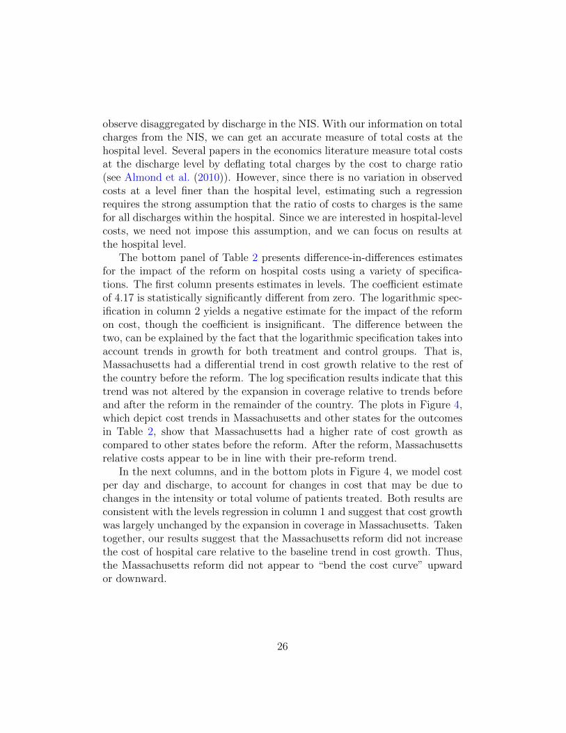
observe disaggregated by discharge in the NIS. With our information on totalcharges from the NIS, we can get an accurate measure of total costs at thehospital level. Several papers in the economics literature measure total costsat the discharge level by deflating total charges by the cost to charge ratio(see Almond et al. (2010)). However, since there is no variation in observedcosts at a level finer than the hospital level, estimating such a regressionrequires the strong assumption that the ratio of costs to charges is the samefor all discharges within the hospital. Since we are interested in hospital-levelcosts, we need not impose this assumption, and we can focus on results atthe hospital level.

The bottom panel of Table 2 presents difference-in-differences estimatesfor the impact of the reform on hospital costs using a variety of specifica-tions. The first column presents estimates in levels. The coefficient estimateof 4.17 is statistically significantly different from zero. The logarithmic spec-ification in column 2 yields a negative estimate for the impact of the reformon cost, though the coefficient is insignificant. The difference between thetwo, can be explained by the fact that the logarithmic specification takes intoaccount trends in growth for both treatment and control groups. That is,Massachusetts had a differential trend in cost growth relative to the rest ofthe country before the reform. The log specification results indicate that thistrend was not altered by the expansion in coverage relative to trends beforeand after the reform in the remainder of the country. The plots in Figure 4,which depict cost trends in Massachusetts and other states for the outcomesin Table 2, show that Massachusetts had a higher rate of cost growth ascompared to other states before the reform. After the reform, Massachusettsrelative costs appear to be in line with their pre-reform trend.

In the next columns, and in the bottom plots in Figure 4, we model costper day and discharge, to account for changes in cost that may be due tochanges in the intensity or total volume of patients treated. Both results areconsistent with the levels regression in column 1 and suggest that cost growthwas largely unchanged by the expansion in coverage in Massachusetts. Takentogether, our results suggest that the Massachusetts reform did not increasethe cost of hospital care relative to the baseline trend in cost growth. Thus,the Massachusetts reform did not appear to “bend the cost curve” upwardor downward.

26

5. Implications for National Reform

While the impact of Massachusetts reform is of intrinsic interest, ourresults are also of broader interest given the similarities between the Mas-sachusetts reform and the national reform. Without far more stringent mod-eling assumptions, it is difficult to predict the impact of coverage expansionsat the national level. Nevertheless, our results do provide some broad pre-dictions for national reform.

We find that the policy tools employed in Massachusetts expanded cover-age among the previously uninsured. In the overall population, roughly halfof new coverage was from private sources and the other half was from sub-sidized sources. Within the hospitalized population, we find some evidencefor crowd-out of private coverage by subsidized coverage. The magnitude ofthe coverage increase under national reform could differ because several pol-icy parameters, such as subsidies and penalties, have different magnitudes.Under national reform, the Congressional Budget Office predicts a reductionin uninsurance of 30 million people or roughly 8.4 percentage points (Con-gressional Budget Office (2012)). This estimate, along with the Centers forMedicare and Medicaid Services estimate of 7.1 percentage points (Trufferet al. (2010)), is slightly larger than reduction in coverage we find in Mas-sachusetts, but they are of a comparable magnitude, suggesting extrapolatingour broad findings is reasonable.

Subject to the caveat that some specific features of the Massachusetts ex-perience that might make our results less valid in predicting the impact of thenational reform, our results suggest that the national reform will likely resultin reductions in length of stay, fewer preventable admissions, and fewer ad-missions from the emergency room. In Massachusetts, declines in admissionsfrom the emergency room are largest among those with the lowest incomes,but Massachusetts is a wealthy state. To the extent that larger and poorerstates have a greater share of the population at lower income levels, the im-pact on ER utilization could be even larger. However, some of our resultscould be specific to the hospital market in Massachusetts. Massachusetts,particularly the Boston area, has many large, prestigious medical centers.It is also a relatively concentrated hospital market. Additional coverage orchanges in insurer market power might have different effects in other settings.

We find that the Massachusetts reform did not lower hospital cost growthin the aggregate. However, cost impacts are likely to be different under na-tional reform. Massachusetts financed health reform largely through the

27

reallocation of money already allocated for specific programs like the uncom-pensated care pool and DSH payments. The national reform also includeschanges in Medicare financing that could affect incentives at the hospitallevel. These changes include payment reductions for Medicare Advantageand the introduction of new payment models including bundled paymentsand Accountable Care Organizations. The latter provides potentially verydifferent incentives for care delivery because it provides incentives for primarycare doctors to lower cost.

6. Conclusion

In this paper, we show that the Massachusetts health insurance reform ex-panded coverage among the inpatient hospital population by approximately36 percent relative to its pre-reform level. Among this population, we seesome evidence of the crowd-out of private coverage by subsidized coverage,but we do not find evidence for crowd-out in the general population, sug-gesting that the incidence of crowd-out differs by health status.

This paper is the first to examine the effect of Massachusetts health in-surance reform on hospital outcomes. We show declines in length of stayand admissions from the emergency room following the reform. Our results,while sensitive to the inclusion of controls for patient severity, also suggestthat prevention increased outside of hospitals, resulting in a decline in inpa-tient admissions for certain preventable conditions, reflecting a likely healthimpact for individuals susceptible to these conditions. In the midst of thesegains, we find no evidence that hospital cost growth increased. We are unableto make precise welfare statements as we do not capture increased costs tothe government and to the purchasers of health insurance that resulted fromthe reform. As our research progresses, we aim to answer other economicsquestions using variation by health insurance reform in Massachusetts.

7. Acknowledgements

Toby Chaiken, Andrew Maleki, Doug Norton, Michael Punzalan, AditiSen, and Swati Yanamadala provided excellent research assistance. C. LanierBenkard, Joseph Doyle, Mark Duggan (the editor), Amy Finkelstein, SherryGlied, Dana Goldman, Jonathan Gruber, Kate Ho, Jill Horwitz, Rob Huck-man, Kosali Simon, Jonathan Skinner, Erin Strumpf, Ebonya Washington,Heidi Williams, and anonymous referees provided helpful feedback. We thank

28

the Schaeffer Center at USC. We also thank seminar participants at theUniversity of Connecticut, Columbia University, the University of Illinois,the University of Lausanne, Case Western, Rice/University of Houston, theNBER Summer Institute, the Louis and Myrtle Moskowitz Workshop onEmpirical Health Law and Business at the University of Michigan, and the2nd HEC Montreal IO and Health Conference. Mohan Ramanujan and JeanRoth provided invaluable support at the NBER. Remaining errors are ourown.

Agency for Healthcare Research and Quality. HCUP Nationwide InpatientSample (NIS). Healthcare Cost and Utilization Project (HCUP). Rockville,MD, April 2004 – 2007. www.hcup-us.ahrq.gov/nisoverview.jsp.

Agency for Healthcare Research and Quality. AHRQ QualityIndicators Software Download. Rockville, MD, April 2007a.http://www.qualityindicators.ahrq.gov/software.htm.

Agency for Healthcare Research and Quality. Pediatric Safety Indica-tors Download. AHRQ Quality Indicators. Rockville, MD, March 2007b.http://www.qualityindicators.ahrq.gov/pqi download.htm.

Douglas Almond, Jr. Joseph J. Doyle, Amanda E. Kowalski, and HeidiWilliams. Estimating Marginal Returns to Medical Care: Evidence fromAt-Risk Newborns. Quarterly Journal of Economics, 125(2):591–634, 2010.

Marianne Bertrand, Esther Duflo, and Sendhil Mullainathan. How MuchShould We Trust Differences-in-Differences Estimates?*. Quarterly Jour-nal of Economics, 119(1):249–275, 2004.

Michael Birnbaum and Elizabeth Patchias. Medicare Coverage for Se-niors: How Universal Is It and What Are the Implications?*. Paperpresented at the annual meeting of the APSA 2008 Annual Meeting,Hynes Convention Center, Boston, Massachusetts, August 28, 2008, 2008.http://www.allacademic.com/meta/p281081 index.html.

David Card, Carlos Dobkin, and Nicole Maestas. The Impact of NearlyUniversal Insurance Coverage on Health Care Utilization: Evidence fromMedicare. American Economic Review, 98(5):2242–2258, 2008.

29

Mary E. Charlson, Peter Pompei, Kathy L. Ales, and C. Ronald MacKen-zie. A New Method of Classifying Prognostic Comorbidity in LongitudinalStudies: Development and Validation. Journal of Chronic Diseases, 40(5):373–383, 1987.

Michael E. Chernew, Allison B. Rosen, and A. Mark Fendrick. Value-BasedInsurance Design. Health Affairs, 26(2):w195, 2007.

Congressional Budget Office. Updated Estimates for the Insurance CoverageProvisions of the Affordable Care Ac, 2012. Douglas Elmendorf, Director.Available at http://www.cbo.gov.

Janet Currie and Jonathan Gruber. Health Insurance Eligibility, Utilizationof Medical Care, and Child Health. The Quarterly Journal of Economics,111(2):431–466, 1996.

David M. Cutler and Jonathan Gruber. Does Public Insurance Crowd OutPrivate Insurance. The Quarterly Journal of Economics, 111(2):391–430,1996.

David M. Cutler, Mark McClellan, and Joseph P. Newhouse. How DoesManaged Care Do It? The RAND Journal of Economics, 31(3):526–548,2000.

David Dranove and Mark A. Satterthwaite. Monopolistic Competition WhenPrice and Quality are Imperfectly Observable. RAND Journal of Eco-nomics, 23(4):518–534, 1992.

Mark G. Duggan. Hospital Ownership and Public Medical Spending. Quar-terly Journal of Economics, 115(4):1343–1373, 2000.

Amy Finkelstein. The Aggregate Effects of Health Insurance: Evidence fromthe Introduction of Medicare. The Quarterly Journal of Economics, 122(1):1–37, 2007.

Amy Finkelstein, Sarah Taubman, Bill Wright, Mira Bernstein, JonathanGruber, Joseph P. Newhouse, Heidi Allen, Katherine Baicker, and theOregon Health Study Group. The Oregon Health Insurance Experiment:Evidence from the First Year. The Quarterly Journal of Economics, pageForthcoming, 2012.

30

Sherry Glied and Joshua Zivin. How Do Doctors Behave When Some (butNot All) of Their Patients are in Managed Care? Journal of Health Eco-nomics, 21(2):337–353, 2002.

April Grady. The Massachusetts Health Reform a Brief Overview. Congres-sional Research Service Report for Congress, 2006.

Bradford H. Gray, Roberta Scheinmann, Peri Rosenfeld, and Ruth Finkel-stein. Aging without Medicare? Evidence from New York City. Inquiry,43(3):211–221, 2006.

Jonathan Gruber and Samuel A. Kleiner. Do Strikes Kill? Evidence fromNew York State. NBER Working Paper 15855, 2010.

HSS, Inc. Definitions Manual for All-Payer Severity-adjusted DRG (APS-DRGs) Assignment. Germantown, MD, 2003. http://www.hcup-us.ahrq.gov/db/nation/nis/APS DRGsDefManualV26Public.pdf.

Paul L. Joskow. The Effects of Competition and Regulation on Hospital BedSupply and the Reservation Quality of the Hospital. The Bell Journal ofEconomics, pages 421–447, 1980.

Kaiser Family Foundation. Side-by-side comparisonof major health care reform proposals, March 2010.http://www.kff.org/healthreform/upload/housesenatebill final.pdf.

Jon Kingsdale. Implementing Health Care Reform in Massachusetts: Strate-gic Lessons Learned. Health Affairs, 28(4):w588, 2009.

Jonathan T. Kolstad and Amanda E. Kowalski. The impact of health care re-form on hospital and preventive care: Evidence from massachusetts. NBERWorking Paper 16012, 2010.

Liz Kowalczyk. Emergency room visits grow in mass. The Boston Globe,July 2010.

Amanda Kowalski. Censored Quantile Instrumental Variable Estimates ofthe Price Elasticity of Expenditure on Medical Care. NBER WorkingPaper 15085, 2009.

Sharon Long. On the Road to Universal Coverage: Impacts of Reform inMassachusetts at One Year. Health Affairs, 27(4):w270, 2008.

31

Sharon K. Long, Karen Stockley, and Alshadye Yemane. Another Look atthe Impacts of Health Reform in Massachusetts: Evidence Using New Dataand a Stronger Model. American Economic Review, 99(2):508, 2009.

Willard G. Manning, Joseph P. Newhouse, Naihua Duan, Emmett Keeler,Bernadette Benjamin, Arleen Leibowitz, M. Susan Marquis, and JackZwanziger. Health Insurance and the Demand for Medical Care: Evi-dence from a Randomized Experiment. The American Economic Review,77(3):251–277, 1987.

John E. McDonough, Brian Rosman, Fawn Phelps, and Melissa Shannon.The Third Wave of Massachusetts Health Care Access Reform. HealthAffairs, 25(6):w420, 2006.

Sarah Miller. The effect of insurance on emergency room visits: An analysisof the 2006 massachusetts health reform. Mimeo, 2011.

Mark V. Pauly. The Economics of Moral Hazard: Comment. The AmericanEconomic Review, pages 531–537, 1968.

Hude Quan, Vijaya Sundararajan, Patricia Halfon, Andrew Fong, BernardBurnand, Jean-Christophe Luthi, Duncan L. Saunders, Cynthia A. Beck,Thomas E. Feasby, and William A. Ghali. Coding Algorithms for DefiningComorbidities in ICD-9-CM and ICD-10 Administrative Data. MedicalCare, 43(11):1130, 2005.

James C. Robinson and Harold S. Luft. Competition and the Cost of HospitalCare, 1972 to 1982. Journal of the American Medical Association, 257(23):3241, 1987.

The Massachusetts Health Insurance Connector Authority. Report to theMassachusetts Legislature: Implementation of the Health Care ReformLaw, Chapter 58, 2006–2008, 2008. Jon Kingsdale, Executive Director.Available at www.mahealthconnector.org.

Christopher J. Truffer, Sean Keehan, Sheila Smith, Jonathan Cylus, AndreaSisko, John A. Poisal, Joseph Lizonitz, and M. Kent Clemens. HealthSpending Projections through 2019: The Recession’s Impact Continues.Health Affairs, 29(3):522, 2010.

32

Aaron Yelowitz and Michael F. Cannon. The Massachusetts HealthPlan: Much Pain, Little Gain. Policy Analysis, January 2010.http://www.cato.org/pub display.php?pub id=11115.

Appendix A. Block Bootstrap

Since our main identifying variation is at the state-time level, we followBertrand et al. (2004), and block bootstrap our confidence intervals by state.Doing so allows for an arbitrary variance-covariance matrix within statesacross time. In this section, we discuss some implementation details thatare not discussed by Bertrand et al. (2004). First, the empirical simulationresults using the CPS presented by Bertrand et al. (2004) assume that halfof the states are treated and the other half are untreated. Since we haveonly one treated state, it is only sampled in approximately one third of blockbootstrap draws. In these draws, the difference-in-differences coefficient onMA∗After cannot be estimated. In practice, we include these replicationsin the bootstrap sample to estimate the confidence intervals on the othercoefficients without bias. We use a large number of bootstrap replications –1,000 – so that the confidence intervals on our coefficient of interest are stillbased on a large number of bootstrap replications.23

Second, all of our regressions are weighted. To address weighting withinour block bootstrap procedure, we sample states with replacement. Within astate, the sum of the weights does not change because all observations from agiven state are drawn at once. However, the sum of the weights varies acrossregressions because not all states are sampled and some states are sampledmore than once.

Appendix B. Robustness of Insurance Results

One potential concern about the external validity of our results is thatMassachusetts could differ from the remainder of the country in ways thatwe do not observe, and these differences could lead to changes in coverage at

23Difficulties in the block bootstrap procedure aside, we acknowledge that having onlyone treated state potentially limits the external validity of our results. To address thislimitation, we consider level and trend differences between MA and other states, which wediscuss in Section 4.1.1.

33

the same time that the reform was implemented. Such differences could bedue, for example, to factors that affected the entire Northeast. Alternately, itcould be due to factors that affected states with relatively low levels of unin-surance. To account for potential unobserved differences that are correlatedwith observed differences in uninsurance, we estimate a series of specifica-tions in our nonelderly sample, in which we restrict the comparison groups tostates most similar to Massachusetts. We present these results in AppendixTable 7.

We first examine changes in uninsurance. When we restrict the compar-ison group of hospitals to hospitals in the Northeast Census division in thesecond panel, the impact of the reform on uninsurance is smaller than it is inthe preferred specification, reproduced in the first panel. As reported in themeans at the bottom of the column, the initial level of insurance coveragein the comparison states in the Northeast Census division was similar to theinitial level of insurance coverage in the comparison states in the nationalsample. Similarly, in the third panel, when we restrict the comparison groupto include only New England states, which had an initial lower but not statis-tically lower rate of uninsurance than Massachusetts, the estimated impactof the reform falls to a 1.59 percentage point reduction in uninsurance. Thisis statistically smaller than the baseline effect, but it remains significantlydifferent from zero at the 1 percent level despite the much smaller samplesize. To investigate the possibility that this change in magnitude is due tothe limited health reforms that occurred in 2006 in Maine, Vermont andSan Francisco, California, in column 4, we estimate the main specificationin the full sample but we exclude Maine, Vermont, and California. Reas-suringly, our point estimate remains unchanged from our main specification.As an alternative specification check, we estimate the same specification onthe sample of the 25 states with the highest levels of nonelderly insurancecoverage before the reform in the CPS. Our point estimate is not statisticallydifferent from that in the main specification.

In the remaining columns of Appendix Table A4, we present similar spec-ifications for each of our main outcomes of interest. In general, our quanti-tative conclusions as well as our qualitative conclusions are unchanged whenwe change the group of comparison states. Our emergency admission resultis particularly robust.

An additional issue in extrapolating from our Massachusetts results isthat Massachusetts had a relatively smaller potential increase in insurancedue to its high baseline level. If the cost of expanding coverage is convex, we

34

expect larger reductions in uninsurance from the same policies in locationswith higher baseline levels of uninsurance. We could test this proposition ifanother state with a different baseline level of uninsurance enacted the samepolicies. In the absence of such a natural experiment, we look for suggestiveevidence in support of this hypothesis by examining the effect of the reformby baseline levels of insurance coverage within Massachusetts on the hospitallevel.

In Appendix Table A5, we divide hospitals based on their initial level ofinsurance coverage in the pre-reform period. Because not all hospitals in thesample were in the pre-reform data, we first restrict the sample to hospitalsthat appear at least once in the sample in the Before period. These results arepresented in the second panel. Estimating the average impact of the reformin this subsample, we find that impact of the reform remained virtuallyunchanged, 1.52 percentage points compared to 1.53. We then divide thesample into two groups based on whether the hospital had below- or above-median levels of uninsurance in the Before period. Among Massachusettshospitals in the sample in the Before period, 29 hospitals had uninsurancebelow the national median, and the remaining 11 hospitals had uninsuranceabove the national median. We are able to estimate statistically significantimpacts on uninsurance in both groups of hospitals, but estimates based onhospitals with below-median uninsurance are more precise.

Estimates from the first column of the third and fourth panels show thatthe impact of the reform was statistically indistinguishable in hospitals withlower initial rates of uninsurance (a 1.78 percentage point increase in cover-age) and hospitals with higher initial rates of uninsurance (a 1.65 percentagepoint increase in coverage). Although we might have expected that convexcost of coverage expansion would have led to greater reductions in uninsur-ance in hospitals with initially higher rates of uninsurance, the results arenot statistically different from each other. As shown in the second to fourthcolumns, impacts on length of stay and admissions from the ER were alsosimilar across both groups of hospitals. Without recovering the structuralparameters that determine the cost of coverage expansion it is difficult tomake precise out of sample predictions. However, these findings suggest theresults we find in Massachusetts, which had lower initial uninsurance thanother states, could be similar to the impact of the national reform.

35

Appendix C. Risk Adjustment

Selection into hospitals after the reform in Massachusetts is an outcomeof interest in its own right, which we address as a complement to our analysis,but to examine causal changes in other outcomes, we control for character-istics of the patient pool. To do so, we use six24 sets of risk adjustment vari-ables: demographic characteristics, the number of diagnoses on the dischargerecord, individual components of the Charlson Score measure of comorbidi-ties, AHRQ comorbidity measures, All-Patient Refined Diagnosis RelatedGroups (APR-DRGs), and All-Payer Severity-adjusted (APS-DRGs). Eachrisk adjustment measure was developed with a slightly different purpose, butthe correlation among them is high. Since our focus is on controlling forselection and not on investigating the relative merit of each measure, we in-clude all risk adjustment variables in the same specification. We run all ofour regressions on the discharge level, as opposed to the hospital level, tocapture the interactions between measures on the discharge level.

We construct the first four measures ourselves from the information inthe discharge records. First, we include the same demographic measuresthat we include in specification 3 of Table 1 – saturated controls in race,gender, and income, as well as age and age squared. Second, following Gruberand Kleiner (2010), we control for the number of diagnoses on the hospitaldischarge record. The number of diagnoses in our nonelderly sample variesfrom 0 to 15, the average is 5, and the maximum potentially reported is 15.Third, using data on the composition of diagnoses, we calculate and controlfor the individual components of the Charlson Score.25 The Charlson score,which includes 18 components, has been shown to have a strong relationshipwith mortality (Quan et al. (2005)). The average number of components inour nonelderly data is 0.37, and the maximum is 9. Fourth, we control forthe 29 AHRQ comorbidity measures. The nonelderly mean in our data is 1and the maximum is 14.

The remaining two measures were constructed in our data using propri-

24In Kolstad and Kowalski (2010), we included a seventh set of risk adjusters, Medstatdisease staging measures, but we must omit them here because they are no longer availablein 2008.

25See Charlson et al. (1987) for the origin of the Charlson Score measures. We drawour Charlson Score code from http://healthservices.cancer.gov/seermedicare/

program/charlson.comorbidity.macro.txt.

36

etary algorithms. The APR-DRG measures and the APS-DRG measures, de-veloped by 3M, were developed as refinements to the existing Refined DRGs(R-DRGs) and All-Patient DRGs (AP-DRGs) systems, which expanded theDRG system beyond the Medicare population. The APR-DRG and APS-DRG measures include further adjustments for severity and for neonatal dis-charges. There are two separate APR-DRG measures: a mortality-specificmeasure and a general severity measure. We include both measures in eachspecification. The mortality measure takes on integer values from 0 to 4 witha mean in our data of 1.3, and the severity measure takes on the same valueswith a mean of 1.7.

There are three APS-DRG measures: one charge-specific measure, onelength of stay-specific measure, and one mortality-specific measure. Eachoutcome-specific APS-DRG measure was developed using the 2000 NIS data,and is standardized to have a mean of 1 in that sample (HSS, Inc. (2003)).Multiplying the outcome-specific measure by the mean of that outcome inthe 2000 NIS gives a prediction of the expected value of that outcome. Forexample, the mean charge in the 2000 NIS was $13,241.41, and the largestvalue of the charge-specific APS-DRG for a discharge in our nonelderly sam-ple was 26.21, so predicted charges for that discharge would be $347,057 inthe year 2000. To interpret the other magnitudes, the mean LOS in the 2000NIS was 4.5096, and mean mortality in the 2000 NIS was 0.0247 deaths perdischarge. In our sample including all ages, the means of each measure areslightly greater than the standardized value of 1.0, reflecting real changes insince the year 2000 and sampling changes from the 2000 NIS to 2004-2007NIS. The charges measure takes on values from 0.09 to 26.21, with a meanof 0.88 in the nonelderly sample; the length of stay measure takes on valuesfrom 0.21 to 19.02, with a mean of 0.93 in the nonelderly sample; and themortality measure takes on values from 0 to 46.74, with a mean of 0.69 in thenonelderly sample. We include all three measures in each specification. Thesecond specification of Appendix Table A3 reports the coefficients on all riskadjustment variables in the risk-adjusted uninsurance regression reported inthe last row of the first specification in Table 1.

Appendix D. Prevention Quality Indicators

We use software from AHRQ to calculate these measures in our NISdata (Agency for Healthcare Research and Quality (2007a)). We use theDecember 2009 Version 4.1 of the Prevention Quality Indicators (Agency

37

for Healthcare Research and Quality (2007b)), the most recent version thatdoes not include a windows executable file. The calculation of each one ofthese quality indicators is often based on a complicated algorithm becausethe diagnosis first needs to be identified, and then specific discharges mustbe excluded based on secondary diagnoses and risk factors that mitigatethe potential for prevention. Each quality measure includes a numerator, aspecific condition, and a denominator, the population at risk for this specificcondition, which sometimes represents the entire population in a geographicarea. The presence of the numerator and denominator allows a researcherto calculate rates with data for a single hospital. Since our research designcompares hospitals to each other and to themselves over time, we do notcalculate any of the measures as rates. Instead, we use a dummy dependentvariable to indicate inclusion in the numerator – the presence of a qualitymeasure on a specific discharge. For each quality measure, we restrict thesample to discharges included in the denominator.

Appendix E. Behavioral Risk Factor Surveillance System (BRFSS)

The BRFSS is a cross-sectional telephone survey conducted by statehealth departments on a monthly basis with technical and methodologicalassistance provided by the Centers for Disease Control (CDC). Sampling fol-lows a multistage design based on random-digit-dialing in order to select arepresentative sample from the non-institutionalized adult population in eachstate and territory. Our sample from BRFSS data contain 2,293,672 obser-vations; in the analysis, data are weighted for the probability of selection ofa telephone number, the number of adults in a household, and the numberof telephones in a household; post-stratification adjustments are also madefor non-response and non-coverage of households without telephones.

Appendix F. Comparison of NIS Hospital Sample to the Universeof Hospitals in Massachusetts

One important question in evaluating our results is the degree to whichthe NIS hospital sample is reflective of the actual distribution of hospitals inMassachusetts. To address this issue, we obtained the detailed data on theuniverse of hospitals in the state of Massachusetts from the MassachusettsDepartment of Health Care Finance and Policy. Appendix Table A6 presentsa comparison of the hospitals in the two samples in 2008, the most recent year

38

of our data. The comparison of means across the two samples demonstratesclearly the similarities between the two. The NIS sample appears to havemore large hospitals than the universe though the average number of beds isrelatively similar. The composition by for-profit and not-for-profit status inthe NIS appears to be highly representative of the universe of discharges, asare most of the variables. This comparison makes clear that while the NISis a sample intended to be nationally representative, in Massachusetts, thedischarges included in the NIS are very reflective of the universe of dischargesin our sample period.

39

Figure 1: Mean Coverage Rates by Year

1

Figure 1

Source: 2004-2009 Supplements to the Current Population Survey, authors’ calculations. Vertical lines

separate During and After periods.

40

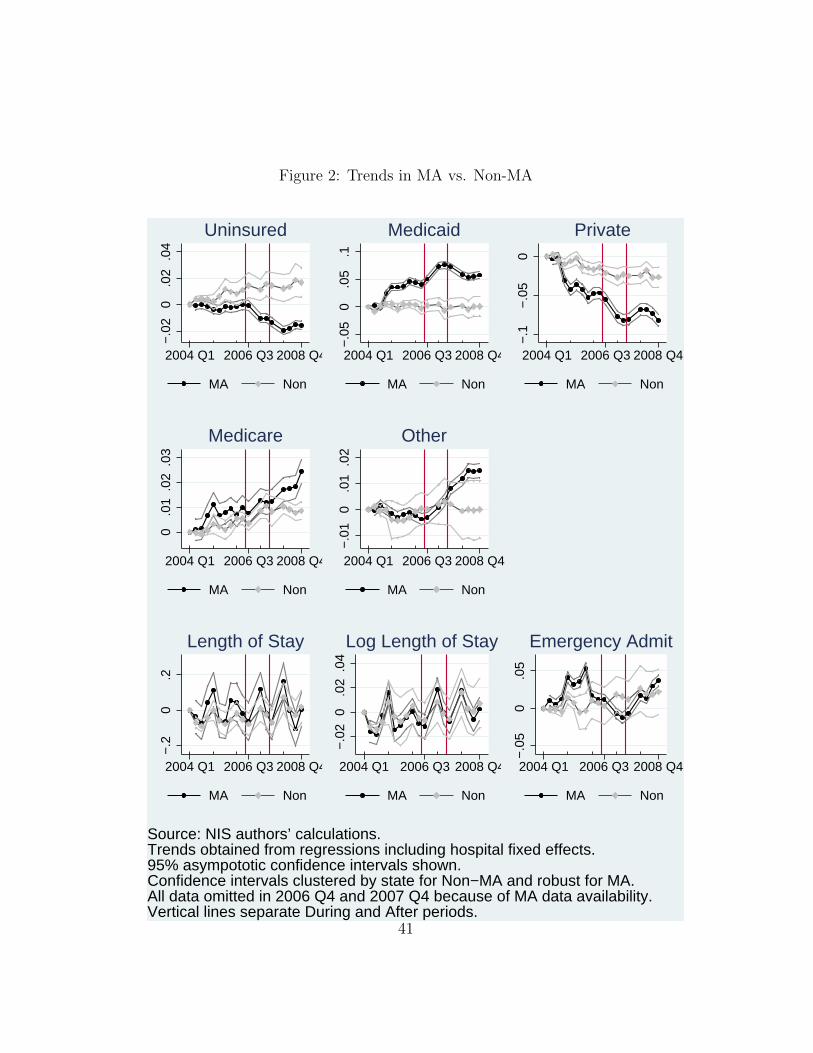
Figure 2: Trends in MA vs. Non-MA−

.02

0.0

2.0

4

2004 Q1 2006 Q3 2008 Q4

MA Non

Uninsured

−.0

50

.05

.12004 Q1 2006 Q3 2008 Q4

MA Non

Medicaid

−.1

−.0

50

2004 Q1 2006 Q3 2008 Q4

MA Non

Private

0.0

1.0

2.0

3

2004 Q1 2006 Q3 2008 Q4

MA Non

Medicare

−.0

10

.01

.02

2004 Q1 2006 Q3 2008 Q4

MA Non

Other

−.2

0.2

2004 Q1 2006 Q3 2008 Q4

MA Non

Length of Stay

−.0

20

.02

.04

2004 Q1 2006 Q3 2008 Q4

MA Non

Log Length of Stay

−.0

50

.05

2004 Q1 2006 Q3 2008 Q4

MA Non

Emergency Admit

Source: NIS authors’ calculations.Trends obtained from regressions including hospital fixed effects.95% asympototic confidence intervals shown.Confidence intervals clustered by state for Non−MA and robust for MA.All data omitted in 2006 Q4 and 2007 Q4 because of MA data availability.Vertical lines separate During and After periods.

Trends in MA vs Non−MA

41

Figure 3: Trends in MA vs. Non-MA, Hospital Quarter Level−

500

050

0

2004 Q1 2006 Q3 2008 Q4

MA Non

Total Discharges

0.2

.42004 Q1 2006 Q3 2008 Q4

MA Non

Charlson Score

−.1

0.1

.2

2004 Q1 2006 Q3 2008 Q4

MA Non

APRDRG Risk Mortality

−.1

0.1

.2

2004 Q1 2006 Q3 2008 Q4

MA Non

APRDRG Severity

−.2

0.2

2004 Q1 2006 Q3 2008 Q4

MA Non

APSDRG Mort. Wei.

−.0

50

.05

2004 Q1 2006 Q3 2008 Q4

MA Non

APSDRG LOS Weight

−.1

−.0

50

.05

2004 Q1 2006 Q3 2008 Q4

MA Non

APSDRG Charge Weight

Source: NIS authors’ calculations.Trends obtained from regressions including hospital fixed effects.95% asympototic confidence intervals shown.Confidence intervals clustered by state for Non−MA and robust for MA.All data omitted in 2006 Q4 and 2007 Q4 because of MA data availability.Vertical lines separate During and After periods.

Trends in MA vs Non−MAHospital−Quarter Level

42

Figure 4: Trends in MA vs. Non-MA, Hospital Quarter Level−

200

2040

2004 Q1 2006 Q3 2008 Q4

MA Non

Total Costs

0.2

.4

2004 Q1 2006 Q3 2008 Q4

MA Non

Log Total Costs

020

040

060

0

2004 Q1 2006 Q3 2008 Q4

MA Non

Costs Per Total LOS0

.1.2

.3

2004 Q1 2006 Q3 2008 Q4

MA Non

Log Costs/LOS

020

0040

00

2004 Q1 2006 Q3 2008 Q4

MA Non

Costs Per Total Discharge

0.1

.2.3

2004 Q1 2006 Q3 2008 Q4

MA Non

Log Costs/Discharge

Source: NIS authors’ calculations.Trends obtained from regressions including hospital fixed effects.95% asympototic confidence intervals shown.Confidence intervals clustered by state for Non−MA and robust for MA.All data omitted in 2006 Q4 and 2007 Q4 because of MA data availability.Vertical lines separate During and After periods.

Trends in MA vs Non−MAHospital−Quarter Level

43

Tab

le1:

Insu

rance

and

Outc

omes

inth

eN

IS

Insu

ranc

e an

d O

utco

mes

in N

IS

(1)

(2)

(3)

(4)

(5)

(6)

(7)

Depe

nden

t Var

iabl

e:U

nins

ured

Med

icai

dPr

ivat

eM

edic

are

Oth

erCo

mm

Care

No

Cove

rage

Info

MA*

Afte

r-0

.023

10.

0389

-0.0

306

0.00

420.

0106

0.01

240.

0015

[-0.0

300,

-0.0

162]

***

[0.0

265,

0.05

12]*

**[-0

.037

8,-0

.023

3]**

*[0

.001

3,0.

0070

]***

[0.0

041,

0.01

71]*

**[0

.012

3,0.

0124

]***

[0.0

000,

0.00

30]*

* [-

0.02

99,-0

.016

6]++

+ [0

.029

3,0.

051]

+++

[-0

.038

5,-0

.023

6]++

+[0

.001

4,0.

0068

]+++

[0

.005

0,0.

0181

]+++

[0.0

124,

0.01

25]+

++

[0.0

001,

0.00

29]+

+

MA*

Durin

g-0

.012

90.

0365

-0.0

224

-0.0

003

-0.0

009

0.00

29-0

.001

7[-0

.017

6,-0

.008

3]**

*[0

.029

3,0.

0437

]***

[-0.0

274,

-0.0

173]

***

[-0.0

024,

0.00

17]

[-0.0

043,

0.00

26]

[0.0

029,

0.00

29]*

**[-0

.006

5,0.

0031

][-0

.017

7,-0

.008

4]++

+[0

.030

2,0.

0438

]+++

[-0

.027

7,-0

.016

8]++

+

[-0.0

025,

0.00

18]

[-0.0

049,

0.00

26]

[0.0

029,

0.00

29]+

++[-0

.007

6,0.

0014

]N

(Non

elde

rly)

23,8

60,9

3023

,860

,930

23,8

60,9

3023

,860

,930

23,8

60,9

3023

,860

,930

23,9

13,9

83R

Squa

red

0.06

590.

1148

0.15

020.

0341

0.06

890.

0249

0.06

62M

ean

MA

Befo

re0.

0643

0.24

600.

5631

0.10

730.

0193

0.00

000.

0002

Mea

n N

on-M

A Be

fore

0.07

910.

2876

0.49

780.

0928

0.04

270.

0000

0.00

20M

ean

MA

Afte

r0.

0352

0.25

940.

5518

0.11

770.

0360

0.01

650.

0040

Mea

n N

on-M

A Af

ter

0.08

170.

2790

0.49

230.

1020

0.04

500.

0000

0.00

17M

A*Af

ter

-0.0

228

0.03

74-0

.027

50.

0021

0.01

070.

0124

0.00

14w

ith ri

sk a

djus

ters

[-0.0

297,

-0.0

158]

***

[0.0

235,

0.05

14]*

**[-0

.036

1,-0

.019

0]**

*[-0

.000

7,0.

0050

][0

.004

7,0.

0168

]***

[0.0

123,

0.01

24]*

**[0

.000

0,0.

0028

]**

R Sq

uare

d0.

0939

0.22

320.

2381

0.20

060.

0761

0.02

490.

0666

(8)

(9)

(10)

Depe

nden

t Var

iabl

e:Le

ngth

of S

tay

Log

Leng

th o

f Sta

yEm

erge

ncy

Adm

itM

A*Af

ter

-0.0

504

-0.0

012

-0.0

202

[-0.0

999,

-0.0

008]

**[-0

.011

1,0.

0086

][-0

.039

7,-0

.000

7]**

[-0.

1026

,-0.0

065]

++[-0

.011

3,0.

0066

][-0

.035

1,0.

0011

]+

MA*

Durin

g-0

.003

70.

0037

-0.0

317

[-0.0

369,

0.02

94]

[-0.0

022,

0.00

95]

[-0.0

449,

-0.0

184]

***

[-0.0

367,

0.02

38]

[-0.0

026,

0.00

84]

[-0.0

409,

-0.0

166]

+++

N (N

onel

derly

)23

,913

,183

23,9

13,1

8323

,913

,983

R Sq

uare

d0.

0335

0.04

580.

1088

Mea

n M

A Be

fore

5.42

561.

4267

0.38

68M

ean

Non

-MA

Befo

re5.

0770

1.35

520.

3591

Mea

n M

A Af

ter

5.37

171.

4355

0.40

58M

ean

Non

-MA

Afte

r5.

0958

1.35

960.

3745

MA*

Afte

r-0

.103

7-0

.010

5-0

.022

0w

ith ri

sk a

djus

ters

[-0.1

471,

-0.0

603]

***

[-0.0

186,

-0.0

023]

**[-0

.042

7,-0

.001

2]**

R Sq

uare

d0.

3801

0.40

380.

2907

95%

asy

mpt

otic

CI c

lust

ered

by

stat

e: *

** S

igni

fican

t at .

01, *

* Si

gnifi

cant

at .

05, *

Sig

nific

ant a

t .10

95%

boo

tstr

appe

d CI

, blo

cks b

y st

ate,

100

0 re

ps: +

++ S

igni

fican

t at .

01, +

+ Si

gnifi

cant

at .

05, +

Sig

nific

ant a

t .10

All s

peci

ficat

ions

and

mea

ns w

eigh

ted

usin

g di

scha

rge

wei

ghts

.Al

l spe

cific

atio

ns in

clud

e ho

spita

l fix

ed e

ffect

s and

tim

e fix

ed e

ffect

s for

200

4 to

200

8, q

uart

erly

.

Com

mCa

re in

clud

ed in

Oth

er.

No

Cove

rage

Info

not

incl

uded

in a

ny o

ther

spec

ifica

tions

.Le

ngth

of S

tay

is c

alcu

late

d as

one

plu

s the

disc

harg

e da

te m

inus

the

adm

issio

n da

te.

The

smal

lest

pos

sible

val

ue is

one

day

. Em

erge

ncy

Adm

it in

dica

tes e

mer

genc

y ro

om so

urce

of a

dmis

sion.

Sour

ce: H

CUP

NIS

200

4-20

08 a

utho

rs' c

alcu

latio

ns.

See

text

for m

ore

deta

ils.

Mut

ually

Exc

lusiv

e Ty

pes o

f Cov

erag

e

Out

com

es

Risk

adj

uste

rs in

clud

e six

sets

of r

isk a

djus

tmen

t var

iabl

es: d

emog

raph

ic c

hara

cter

istic

s, th

e nu

mbe

r of d

iagn

oses

on

the

disc

harg

e re

cord

, ind

ivid

ual c

ompo

nent

s of t

he C

harls

on S

core

m

easu

re o

f com

orbi

ditie

s, A

HRQ

com

orbi

dity

mea

sure

s, A

ll-Pa

tient

Ref

ined

(APR

)-DRG

s, a

nd A

ll-Pa

yer S

ever

ity-a

djus

ted

(APS

)-DRG

s. S

ee A

ppen

dix

2.

44

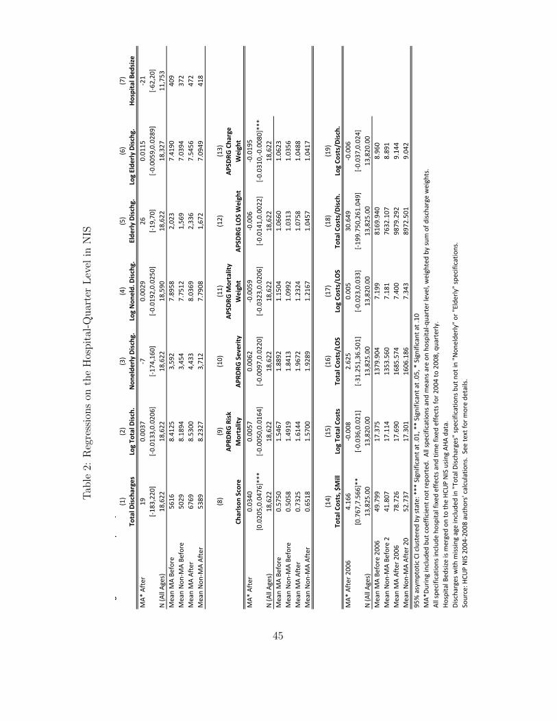
Tab

le2:

Reg

ress

ions

onth

eH

ospit

al-Q

uar

ter

Lev

elin

NIS

Regr

essi

ons

on th

e H

ospi

tal-Q

uart

er L

evel

in N

IS(1

)(2

)(3

)(4

)(5

)(6

)(7

)To

tal D

isch

arge

sLo

g To

tal D

isch

.N

onel

derly

Dis

chg.

Log

Non

eld.

Dis

chg.

Elde

rly D

isch

g.Lo

g El

derly

Dis

chg.

Hos

pita

l Bed

size

MA*

Aft

er19

0.00

37-7

0.00

2926

0.01

15-2

1[-1

83,2

20]

[-0.0

133,

0.02

06]

[-174

,160

][-0

.019

2,0.

0250

][-1

9,70

][-0

.005

9,0.

0289

][-6

2,20

]N

(All

Ages

)18

,622

18,6

2218

,622

18,5

9018

,622

18,3

2711

,753

Mea

n M

A Be

fore

5616

8.41

253,

592

7.89

582,

023

7.41

9040

9M

ean

Non

-MA

Befo

re50

298.

1894

3,45

47.

7512

1,56

97.

0394

372

Mea

n M

A Af

ter

6769

8.53

004,

433

8.03

692,

336

7.54

5647

2M

ean

Non

-MA

Afte

r53

898.

2327

3,71

27.

7908

1,67

27.

0949

418

(8)

(9)

(10)

(11)

(12)

(13)

Char

lson

Sco

reAP

RDRG

Ris

k M

orta

lity

APRD

RG S

ever

ityAP

SDRG

Mor

talit

y W

eigh

tAP

SDRG

LO

S W

eigh

tAP

SDRG

Cha

rge

Wei

ght

MA*

Aft

er0.

0340

0.00

570.

0062

-0.0

059

-0.0

06-0

.019

5[0

.020

5,0.

0476

]***

[-0.0

050,

0.01

64]

[-0.0

097,

0.02

20]

[-0.0

323,

0.02

06]

[-0.0

141,

0.00

22]

[-0.0

310,

-0.0

080]

***

N (A

ll Ag

es)

18,6

2218

,622

18,6

2218

,622

18,6

2218

,622

Mea

n M

A Be

fore

0.57

501.

5467

1.88

921.

1504

1.06

601.

0623

Mea

n N

on-M

A Be

fore

0.50

581.

4919

1.84

131.

0992

1.03

131.

0356

Mea

n M

A Af

ter

0.73

251.

6144

1.96

721.

2324

1.07

581.

0488

Mea

n N

on-M

A Af

ter

0.65

181.

5700

1.92

891.

2167

1.04

571.

0417

(14)

(15)

(16)

(17)

(18)

(19)

Tota

l Cos

ts, $

Mill

Log

Tota

l Cos

tsTo

tal C

osts

/LO

SLo

g Co

sts/

LOS

Tota

l Cos

ts/D

isch

.Lo

g Co

sts/

Dis

ch.

MA*

Aft

er 2

006

4.16

6-0

.008

2.62

50.

005

30.6

49-0

.006

[0.7

67,7

.566

]**

[-0.0

36,0

.021

][-3

1.25

1,36

.501

][-0

.023

,0.0

33]

[-199

.750

,261

.049

][-0

.037

,0.0

24]

N (A

ll Ag

es)

13,8

25.0

013

,820

.00

13,8

25.0

013

,820

.00

13,8

25.0

013

,820

.00

Mea

n M

A Be

fore

200

649

.799

17.3

7513

79.9

047.

199

8169

.940

8.96

0M

ean

Non

-MA

Befo

re 2

41.8

0717

.114

1353

.560

7.18

176

32.1

078.

891

Mea

n M

A Af

ter 2

006

78.7

2617

.690

1685

.574

7.40

098

79.2

929.

144

Mea

n N

on-M

A Af

ter 2

0052

.737

17.3

0116

06.1

867.

343

8972

.501

9.04

295

% a

sym

ptot

ic C

I clu

ster

ed b

y st

ate:

***

Sig

nific

ant a

t .01

, **

Sign

ifica

nt a

t .05

, * S

igni

fican

t at .

10M

A*Du

ring

incl

uded

but

coe

ffici

ent n

ot re

port

ed.

All s

peci

ficat

ions

and

mea

ns a

re o

n ho

spita

l-qua

rter

leve

l, w

eigh

ted

by su

m o

f disc

harg

e w

eigh

ts.

All s

peci

ficat

ions

incl

ude

hosp

ital f

ixed

effe

cts a

nd ti

me

fixed

effe

cts f

or 2

004

to 2

008,

qua

rter

ly.

Hosp

ital B

edsiz

e is

mer

ged

on to

the

HCU

P N

IS u

sing

AHA

data

.Di

scha

rges

with

miss

ing

age

incl

uded

in "

Tota

l Disc

harg

es"

spec

ifica

tions

but

not

in "

Non

elde

rly"

or "

Elde

rly"

spec

ifica

tions

.So

urce

: HCU

P N

IS 2

004-

2008

aut

hors

' cal

cula

tions

. Se

e te

xt fo

r mor

e de

tails

.

45

Tab

le3:

Pre

venti

onQ

ual

ity

Indic

ator

sin

the

NIS

Prev

entio

n Q

ualit

y In

dica

tors

Impr

ovem

ent?

Impr

ovem

ent?

N, M

ean

MA

Befo

rePQ

I 90

Ove

rall

PQI

-0.0

002

[-0.0

016,

0.00

11]

Y-0

.002

3[-0

.003

6,-0

.000

9]**

*17

,674

,454

0.08

38PQ

I 01

Diab

etes

Sho

rt-t

erm

Com

p. A

dmiss

ion

-0.0

001

[-0.0

002,

0.00

01]

-0.0

002

[-0.0

005,

0.00

01]

17,6

74,4

540.

0058

PQI 0

2 Pe

rfor

ated

App

endi

x Ad

miss

ion

Rate

Y-0

.046

3[-0

.055

7,-0

.036

8]**

*Y

-0.0

072

[-0.0

133,

-0.0

012]

**18

9,58

80.

2457

PQI 0

3 Di

abet

es L

ong-

Term

Com

p. A

dmiss

ion

0.00

00[-0

.000

2,0.

0003

]Y

-0.0

009

[-0.0

011,

-0.0

007]

***

17,6

74,4

540.

0083

PQI 0

5 CO

PD A

dmiss

ion

Rate

-0.0

002

[-0.0

005,

0.00

01]

Y-0

.000

5[-0

.000

8,-0

.000

2]**

*17

,674

,454

0.00

97PQ

I 07

Hype

rten

sion

Adm

issio

n ra

te0.

0001

[-0.0

002,

0.00

04]

0.00

01[-0

.000

2,0.

0004

]17

,674

,454

0.00

20PQ

I 08

CHF

Adm

issio

n Ra

te0.

0000

[-0.0

005,

0.00

05]

-0.0

003

[-0.0

006,

0.00

01]

17,6

74,4

540.

0109

PQI 1

0 De

hydr

atio

n Ad

miss

ion

Rate

0.00

00[-0

.000

2,0.

0002

]Y

-0.0

005

[-0.0

007,

-0.0

003]

***

17,6

74,4

540.

0054

PQI 1

1 Ba

cter

ial P

neum

onia

Adm

issio

n Ra

te0.

0001

[-0.0

005,

0.00

06]

0.00

04[-0

.000

2,0.

0009

]17

,674

,454

0.01

72PQ

I 12

Urin

ary

Trac

t Inf

ectio

n Ad

miss

ion

Rate

-0.0

001

[-0.0

004,

0.00

02]

0.00

00[-0

.000

3,0.

0003

]17

,674

,454

0.00

70PQ

I 13

Angi

na w

ithou

t Pro

cedu

re A

dmiss

ion

Rate

N0.

0005

[0.0

004,

0.00

07]*

**N

0.00

05[0

.000

4,0.

0007

]***

17,6

74,4

540.

0014

PQI 1

4 U

ncon

trol

led

Diab

etes

Adm

issio

n ra

te0.

0001

[-0.0

001,

0.00

03]

-0.0

001

[-0.0

003,

0.00

01]

17,6

74,4

540.

0007

PQI 1

5 Ad

ult A

sthm

a Ad

miss

ion

Rate

Y-0

.000

6[-0

.000

9,-0

.000

2]**

*Y

-0.0

006

[-0.0

009,

-0.0

003]

***

17,6

74,4

540.

0146

PQI 1

6 Ra

te o

f Low

er-e

xtre

mity

Am

puta

tion

Y-0

.000

5[-0

.000

6,-0

.000

4]**

*Y

-0.0

006

[-0.0

007,

-0.0

005]

***

17,6

74,4

540.

0023

95%

asy

mpt

otic

CI c

lust

ered

by

stat

e: *

** S

igni

fican

t at .

01, *

* Si

gnifi

cant

at .

05, *

Sig

nific

ant a

t .10

Y an

d N

indi

cate

stat

istic

ally

sign

ifica

nt g

ains

and

loss

es, r

espe

ctiv

ely.

MA*

Durin

g in

clud

ed b

ut c

oeffi

cien

t not

repo

rted

. Al

l spe

cific

atio

ns a

nd m

eans

are

wei

ghte

d us

ing

disc

harg

e w

eigh

ts.

All s

peci

ficat

ions

incl

ude

hosp

ital f

ixed

effe

cts a

nd ti

me

fixed

effe

cts f

or 2

004

to 2

008,

qua

rter

ly.

Regr

essio

ns in

this

tabl

e es

timat

ed in

the

sam

ple

of n

onel

derly

disc

harg

es.

Sour

ce: H

CUP

NIS

200

4-20

08 a

utho

rs' c

alcu

latio

ns.

See

text

for m

ore

deta

ils.

Risk

adj

uste

rs in

clud

e six

sets

of r

isk a

djus

tmen

t var

iabl

es: d

emog

raph

ic c

hara

cter

istic

s, th

e nu

mbe

r of d

iagn

oses

on

the

disc

harg

e re

cord

, ind

ivid

ual c

ompo

nent

s of t

he

Char

lson

Scor

e m

easu

re o

f com

orbi

ditie

s, A

HRQ

com

orbi

dity

mea

sure

s, A

ll-Pa

tient

Ref

ined

(APR

)-DRG

s, a

nd A

ll-Pa

yer S

ever

ity-a

djus

ted

(APS

)-DRG

s. S

ee A

ppen

dix

2.

Prev

entio

n Q

ualit

y In

dica

tors

in th

e N

ISM

A* A

fter

MA*

Aft

er, R

isk

Adju

sted

46

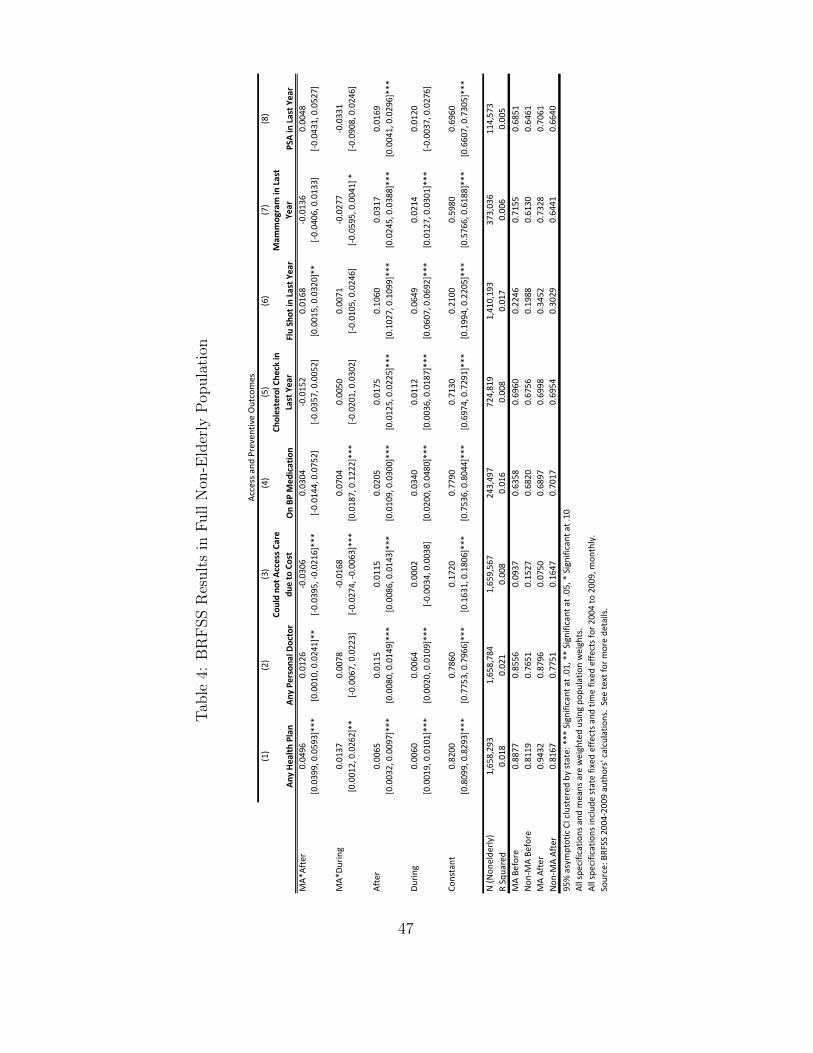
Tab

le4:

BR

FSS

Res

ult

sin

Full

Non

-Eld

erly

Pop

ula

tion

(1)

(2)

(3)

(4)

(5)

(6)

(7)

(8)

Any

Hea

lth P

lan

Any

Pers

onal

Doc

tor

Coul

d no

t Acc

ess C

are

due

to C

ost

On

BP M

edic

atio

nCh

oles

tero

l Che

ck in

La

st Y

ear

Flu

Shot

in L

ast Y

ear

Mam

mog

ram

in L

ast

Year

PSA

in L

ast Y

ear

MA*

Afte

r0.

0496

0.01

26-0

.030

60.

0304

-0.0

152

0.01

68-0

.013

60.

0048

[0.0

399,

0.0

593]

***

[0.0

010,

0.0

241]

**[-0

.039

5, -0

.021

6]**

*[-0

.014

4, 0

.075

2][-0

.035

7, 0

.005

2][0

.001

5, 0

.032

0]**

[-0.0

406,

0.0

133]

[-0.0

431,

0.0

527]

MA*

Durin

g0.

0137

0.00

78-0

.016

80.

0704

0.00

500.

0071

-0.0

277

-0.0

331

[0.0

012,

0.0

262]

**[-0

.006

7, 0

.022

3][-0

.027

4, -0

.006

3]**

*[0

.018

7, 0

.122

2]**

*[-0

.020

1, 0

.030

2][-0

.010

5, 0

.024

6][-0

.059

5, 0

.004

1] *

[-0.0

908,

0.0

246]

Afte

r0.

0065

0.01

150.

0115

0.02

050.

0175

0.10

600.

0317

0.01

69[0

.003

2, 0

.009

7]**

*[0

.008

0, 0

.014

9]**

*[0

.008

6, 0

.014

3]**

*[0

.010

9, 0

.030

0]**

*[0

.012

5, 0

.022

5]**

*[0

.102

7, 0

.109

9]**

*[0

.024

5, 0

.038

8]**

*[0

.004

1, 0

.029

6]**

*

Durin

g0.

0060

0.00

640.

0002

0.03

400.

0112

0.06

490.

0214

0.01

20[0

.001

9, 0

.010

1]**

*[0

.002

0, 0

.010

9]**

*[-0

.003

4, 0

.003

8][0

.020

0, 0

.048

0]**

*[0

.003

6, 0

.018

7]**

*[0

.060

7, 0

.069

2]**

*[0

.012

7, 0

.030

1]**

*[-0

.003

7, 0

.027

6]

Cons

tant

0.82

000.

7860

0.17

200.

7790

0.71

300.

2100

0.59

800.

6960

[0.8

099,

0.8

293]

***

[0.7

753,

0.7

966]

***

[0.1

631,

0.1

806]

***

[0.7

536,

0.8

044]

***

[0.6

974,

0.7

291]

***

[0.1

994,

0.2

205]

***

[0.5

766,

0.6

188]

***

[0.6

607,

0.7

305]

***

N (N

onel

derly

)1,

658,

293

1,65

8,78

41,

659,

567

243,

497

724,

819

1,41

0,19

337

3,03

611

4,57

3R

Squa

red

0.01

80.

021

0.00

80.

016

0.00

80.

017

0.00

60.

005

MA

Befo

re0.

8877

0.85

560.

0937

0.63

580.

6960

0.22

460.

7155

0.68

51N

on-M

A Be

fore

0.81

190.

7651

0.15

270.

6820

0.67

560.

1988

0.61

300.

6461

MA

Afte

r0.

9432

0.87

960.

0750

0.68

970.

6998

0.34

520.

7328

0.70

61N

on-M

A Af

ter

0.81

670.

7751

0.16

470.

7017

0.69

540.

3029

0.64

410.

6640

95%

asy

mpt

otic

CI c

lust

ered

by

stat

e: *

** S

igni

fican

t at .

01, *

* Si

gnifi

cant

at .

05, *

Sig

nific

ant a

t .10

All s

peci

ficat

ions

and

mea

ns a

re w

eigh

ted

usin

g po

pula

tion

wei

ghts

.Al

l spe

cific

atio

ns in

clud

e st

ate

fixed

effe

cts a

nd ti

me

fixed

effe

cts f

or 2

004

to 2

009,

mon

thly

.So

urce

: BRF

SS 2

004-

2009

aut

hors

' cal

cula

tions

. Se

e te

xt fo

r mor

e de

tails

.

Insu

ranc

e an

d ou

tcom

es in

BRF

SSAc

cess

and

Pre

vent

ive

Out

com

es

47

Tab

le5:

Insu

rance

and

Outc

omes

by

Inco

me

inN

IS

Insu

ranc

e an

d O

utco

mes

by

Inco

me

in N

IS(1

)(2

)(3

)(4

)(5

)(6

)(7

)(8

)(9

)U

nins

ured

Med

icai

dPr

ivat

eM

edic

are

Oth

erCo

mm

Care

Leng

th o

f Sta

yLo

g Le

ngth

of S

tay

Emer

genc

y Ad

mit

Patie

nt's

Zip

Cod

e in

Firs

t (Lo

wes

t) In

com

e Q

uart

ile (2

8% o

f sam

ple)

Ma*

Afte

r-0

.035

90.

1050

-0.0

899

0.00

590.

0148

0.01

300.

0535

0.01

58-0

.057

0[-0

.044

0,-0

.027

7]**

*[0

.087

3,0.

1227

]***

[-0.1

004,

-0.0

793]

***

[0.0

025,

0.00

93]*

**[0

.003

5,0.

0260

]**

[0.0

130,

0.01

30]*

**[-0

.005

0,0.

1119

]*[0

.007

1,0.

0244

]***

[-0.0

703,

-0.0

436]

***

Mea

n M

A Be

fore

0.06

430.

2460

0.56

310.

1073

0.01

930.

0000

5.60

741.

4402

0.46

65

Patie

nt's

Zip

Cod

e in

Sec

ond

Inco

me

Qua

rtile

(26%

of s

ampl

e)M

a*Af

ter

-0.0

226

0.04

47-0

.049

50.

0148

0.01

260.

0165

-0.0

941

-0.0

081

-0.0

190

[-0.0

309,

-0.0

143]

***

[0.0

305,

0.05

90]*

**[-0

.059

5,-0

.039

6]**

*[0

.011

3,0.

0184

]***

[0.0

053,

0.01

99]*

**[0

.016

4,0.

0165

]***

[-0.1

310,

-0.0

572]

***

[-0.0

153,

-0.0

009]

**[-0

.029

7,-0

.008

3]**

*M

ean

MA

Befo

re0.

0643

0.24

600.

5631

0.10

730.

0193

0.00

005.

5681

1.44

510.

4437

Patie

nt's

Zip

Cod

e in

Thi

rd In

com

e Q

uart

ile (2

3% o

f sam

ple)

Ma*

Afte

r-0

.023

40.

0217

-0.0

106

0.00

200.

0103

0.01

30-0

.089

00.

0017

-0.0

107

[-0.0

295,

-0.0

174]

***

[0.0

098,

0.03

36]*

**[-0

.018

7,-0

.002

6]**

[-0.0

010,

0.00

50]

[0.0

069,

0.01

38]*

**[0

.013

0,0.

0130

]***

[-0.1

417,

-0.0

363]

***

[-0.0

061,

0.00

95]

[-0.0

392,

0.01

78]

Mea

n M

A Be

fore

0.06

430.

2460

0.56

310.

1073

0.01

930.

0000

5.38

851.

4240

0.36

71

Patie

nt's

Zip

Cod

e in

Fou

rth

(Hig

hest

) Inc

ome

Qua

rtile

(21%

of s

ampl

e)M

a*Af

ter

-0.0

059

0.00

060.

0010

-0.0

007

0.00

500.

0090

-0.0

911

-0.0

185

0.00

98[-0

.015

9,0.

0042

][-0

.008

0,0.

0093

][-0

.011

6,0.

0135

][-0

.006

6,0.

0051

][0

.001

1,0.

0089

]**

[0.0

090,

0.00

90]*

**[-0

.195

7,0.

0136

]*[-0

.047

8,0.

0108

][-0

.032

4,0.

0519

]M

ean

MA

Befo

re0.

0643

0.24

600.

5631

0.10

730.

0193

0.00

005.

2333

1.40

670.

3189

95%

asy

mpt

otic

CI c

lust

ered

by

stat

e: *

** S

igni

fican

t at .

01, *

* Si

gnifi

cant

at .

05, *

Sig

nific

ant a

t .10

MA*

Durin

g in

clud

ed b

ut c

oeffi

cien

t not

repo

rted

. Al

l spe

cific

atio

ns a

nd m

eans

wei

ghte

d us

ing

disc

harg

e w

eigh

ts.

All s

peci

ficat

ions

incl

ude

hosp

ital f

ixed

effe

cts a

nd ti

me

fixed

effe

cts f

or 2

004

to 2

008,

qua

rter

ly.

Regr

essio

ns in

this

tabl

e es

timat

ed in

the

sam

ple

of n

onel

derly

disc

harg

es.

Sam

ple

sizes

var

y ac

ross

spec

ifica

tions

bas

ed o

n av

aila

bilit

y of

dep

ende

nt v

aria

ble.

Resu

lts fo

r miss

ing

gend

er a

nd in

com

e ca

tego

ries n

ot sh

own.

Sour

ce: H

CUP

NIS

200

4-20

08 a

utho

rs' c

alcu

latio

ns.

See

text

for m

ore

deta

ils.

48

Tab

leA

1:In

sura

nce

inC

PS

Insurance in CPS

(1)

(2)

(3)

(4)

(5)

(6)

Uninsured

ESHI

Private Insurance 

Unrelated

 to 

Employmen

tMed

icaid

Med

icare

VA/M

ilitary

MA*

After

‐0.057

10.03

45‐0.008

60.03

51‐0.000

4‐0.003

6[‐0

.060

5,‐0.053

7]***

[0.028

3,0.04

08]***

[‐0.010

6,‐0.006

6]***

[0.031

7,0.03

86]***

[‐0.001

2,0.00

04]

[‐0.005

0,‐0.002

3]***

[‐0.060

4,‐0.053

6]+++ 

[0.028

6,0.04

03]+++

[‐0.010

5,‐0.006

6]+++

[0.031

7,0.03

85]+++

[‐0.001

1,0.00

04]

[‐0.005

1,‐0.002

5]+++

MA*

Durin

g‐0.004

90.00

240.00

66‐0.000

50.00

11‐0.004

7[‐0

.009

3,‐0.000

5]**

[‐0.001

6,0.00

64]

[0.003

6,0.00

96]***

[‐0.003

6,0.00

25]

[0.000

4,0.00

19]***

[‐0.006

1,‐0.003

4]***

[‐0.009

7,‐0.000

5]++

[‐0.002

0,0.00

60]

[0.004

1,0.01

02]+++

[‐0.003

6,0.00

22]

[0.000

4,0.00

19]+++

[‐0.006

,‐0.003

2]+++

After

0.00

07‐0.013

4‐0.000

60.01

010.00

230.00

09[‐0

.002

7,0.00

42]

[‐0.019

7,‐0.007

2]***

[‐0.002

6,0.00

15]

[0.006

6,0.01

36]***

[0.001

5,0.00

31]***

[‐0.000

4,0.00

22]

[‐0.002

7,0.00

37]

[‐0.019

2,‐0.007

7][‐0

.002

5,0.00

13]+

[0.006

8,0.01

35]+++

[0.001

6,0.00

3]+++

[‐0.000

3,0.00

23]+

Durin

g0.00

58‐0.007

7‐0.000

40.00

230.00

10‐0.000

9[0.001

4,0.01

01]**

[‐0.011

7,‐0.003

7]***

[‐0.003

4,0.00

25]

[‐0.000

8,0.00

53]

[0.000

2,0.00

18]**

[‐0.002

2,0.00

04]

[0.001

5,0.01

05]+++

[‐0.011

3,‐0.003

3]+++

[‐0.003

9,0.00

20]+

[‐0.000

4,0.00

53]

[0.000

3,0.00

18]+++

[‐0.002

4,0.00

03]+  

Constant

0.15

110.65

310.04

590.11

950.01

720.01

32[0.149

4,0.15

27]***

[0.650

8,0.65

55]***

[0.045

0,0.04

67]***

[0.118

0,0.12

10]***

[0.016

9,0.01

75]***

[0.012

7,0.01

37]***

[0.116

4,0.18

89]+++

[0.592

2,0.68

98]+++

[0.044

9,0.11

38]+++

[0.067

,0.179

6]+++

 [0.004

1,0.01

75]+++

[0.006

5,0.07

08]+++

 N (N

onelde

rly)

1,12

9,22

11,12

9,22

11,12

9,22

11,12

9,22

11,12

9,22

11,12

9,22

1R Squared

0.01

520.01

600.00

300.00

710.00

130.00

66MA Be

fore

0.11

760.70

440.05

340.11

130.00

570.00

76Non

‐MA Be

fore

0.17

320.63

580.06

070.10

660.00

900.01

47MA After

0.06

120.72

550.04

420.15

650.00

770.00

49Non

‐MA After

0.17

470.62

140.06

020.11

670.01

130.01

5795

% asymptotic CI clustered

 by state: ***

 Significant a

t .01

, ** Significant at .05

, * Significant a

t .10

95% boo

tstrappe

d CI, blocks b

y state, 100

0 reps: +++

 Significant a

t .01

, ++ Significant at .05

, + Significant a

t .10

All spe

cifications and

 means weighted using sample weights.

All spe

cifications includ

e state fixed

 effe

cts a

nd time fixed

 effe

cts for 200

4 to 200

9, ann

ually.  Omitted

 state: Alabama.

Source: C

PS M

arch Sup

plem

ent 2

004‐20

09 autho

rs' calculatio

ns.  See text fo

r more de

tails.

Mutually Exclusiv

e Type

s of C

overage

49

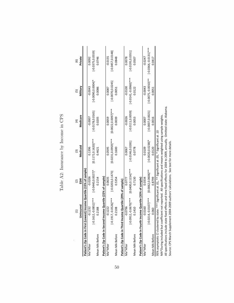
Tab

leA

2:In

sura

nce

by

Inco

me

inC

PS

Insu

ranc

e by

Inco

me

in C

PS(1

)(2

)(3

)(4

)(5

)(6

)U

nins

ured

ESH

IM

edic

aid

Med

icar

eM

ilita

ryPr

ivat

ePa

tient

's Z

ip C

ode

in F

irst (

Low

est)

Inco

me

Qua

rtile

(15%

of s

ampl

e)M

a*Af

ter

-0.1

232

-0.0

206

0.13

96-0

.000

7-0

.004

30.

0092

[-0.1

612,

-0.0

852]

***

[-0.0

440,

0.00

27]*

[0.1

172,

0.16

20]*

**[-0

.017

8,0.

0165

][-0

.009

0,0.

0004

]*[-0

.037

5,0.

0559

]M

ean

MA

Befo

re0.

2188

0.21

540.

4621

0.02

050.

0086

0.07

46

Patie

nt's

Zip

Cod

e in

Sec

ond

Inco

me

Qua

rtile

(22%

of s

ampl

e)M

a*Af

ter

-0.1

222

0.06

350.

0595

0.00

590.

0087

-0.0

155

[-0.1

917,

-0.0

526]

***

[-0.0

203,

0.14

73]

[0.0

231,

0.09

59]*

**[0

.002

2,0.

0097

]***

[-0.0

070,

0.02

45]

[-0.0

457,

0.01

48]

Mea

n M

A Be

fore

0.21

080.

5354

0.16

000.

0039

0.00

510.

0848

Patie

nt's

Zip

Cod

e in

Thi

rd In

com

e Q

uart

ile (2

9% o

f sam

ple)

Ma*

Afte

r-0

.079

60.

0777

0.00

67-0

.002

6-0

.010

00.

0078

[-0.0

912,

-0.0

679]

***

[0.0

400,

0.11

54]*

**[-0

.014

6,0.

0281

][-0

.011

1,0.

0059

][-0

.014

1,-0

.006

0]**

*[-0

.019

5,0.

0351

]M

ean

MA

Befo

re0.

1410

0.71

300.

0778

0.00

530.

0122

0.05

07

Patie

nt's

Zip

Cod

e in

Fou

rth

Inco

me

Qua

rtile

(33%

of s

ampl

e)M

a*Af

ter

-0.0

160

0.03

340.

0109

0.00

07-0

.004

3-0

.024

7[-0

.021

4,-0

.010

7]**

*[0

.006

2,0.

0606

]**

[-0.0

020,

0.02

38]*

[-0.0

007,

0.00

21]

[-0.0

075,

-0.0

010]

**[-0

.036

4,-0

.013

1]**

*M

ean

MA

Befo

re0.

060

0.87

990.

0120

0.00

160.

0051

0.04

1795

% a

sym

ptot

ic C

I clu

ster

ed b

y st

ate:

***

Sig

nific

ant a

t .01

, **

Sign

ifica

nt a

t .05

, * S

igni

fican

t at .

10M

A*Du

ring

incl

uded

but

coe

ffici

ent n

ot re

port

ed.

All s

peci

ficat

ions

and

mea

ns w

eigh

ted

usin

g sa

mpl

e w

eigh

ts.

All s

peci

ficat

ions

incl

ude

stat

e fix

ed e

ffect

s and

tim

e fix

ed e

ffect

s for

200

4 to

200

9, a

nnua

lly.

Om

itted

stat

e: A

laba

ma.

Sour

ce: C

PS M

arch

Sup

plem

ent 2

004-

2009

aut

hors

' cal

cula

tions

. Se

e te

xt fo

r mor

e de

tails

.

50

Tab

leA

3:C

oeffi

cien

tson

Sel

ecte

dC

ovar

iate

sin

NIS

Coef

ficie

nts o

n Se

lect

ed C

ovar

iate

s in

NIS

(1) (

pref

erre

d)(2

) (co

varia

tes)

(2) (

cova

riate

s con

t.)(2

) (co

varia

tes c

ont.)

(2) (

cova

riate

s con

t.)De

pend

ent V

aria

ble

Uni

nsur

edU

nins

ured

Ma*

Afte

r-0

.023

1-0

.022

8Fe

mal

e-0

.039

4AH

RQ C

omor

b.-0

.022

0Ch

arlso

n 6

0.02

55[-0

.030

0,-0

.016

2]**

*[-0

.029

7,-0

.015

8]**

*[-0

.045

3,-0

.033

6]**

*cm

_dm

cx[-0

.027

9,-0

.016

1]**

*[0

.020

1,0.

0308

]***

MA*

Durin

g-0

.012

9-0

.013

1Ge

nder

Unk

now

n-0

.005

8AH

RQ C

omor

b.0.

0720

Char

lson

70.

0086

[-0.0

176,

-0.0

083]

***

[-0.0

177,

-0.0

085]

***

[-0.0

256,

0.01

39]

cm_d

rug

[0.0

506,

0.09

33]*

**[0

.004

7,0.

0124

]***

2004

Q2

0.00

410.

0036

Blac

k0.

0067

AHRQ

Com

orb.

-0.0

009

Char

lson

8-0

.033

3[0

.002

5,0.

0058

]***

[0.0

022,

0.00

50]*

**[0

.001

9,0.

0115

]***

cm_h

tn_c

[-0.0

028,

0.00

10]

[-0.0

407,

-0.0

258]

***

2004

Q3

0.00

440.

0037

Hisp

anic

0.03

62AH

RQ C

omor

b.-0

.011

5Ch

arlso

n 9

0.00

63[0

.002

4,0.

0065

]***

[0.0

018,

0.00

56]*

**[0

.015

9,0.

0565

]***

cm_h

ypot

hy[-0

.014

2,-0

.008

7]**

*[0

.002

0,0.

0107

]***

2004

Q4

0.00

380.

0037

Asia

n0.

0187

AHRQ

Com

orb.

0.00

44Ch

arlso

n 10

0.05

58[0

.001

1,0.

0065

]***

[0.0

010,

0.00

64]*

**[0

.013

4,0.

0240

]***

cm_l

iver

[0.0

004,

0.00

84]*

*[0

.042

7,0.

0689

]***

2005

Q1

0.00

200.

0025

Nat

ive

Amer

ican

0.00

08AH

RQ C

omor

b.-0

.033

2Ch

arlso

n 11

0.01

30[-0

.003

4,0.

0074

][-0

.002

7,0.

0077

][-0

.012

0,0.

0137

]cm

_lym

ph[-0

.040

8,-0

.025

6]**

*[0

.007

1,0.

0189

]***

2005

Q2

0.00

590.

0062

Oth

er R

ace

0.03

53AH

RQ C

omor

b.0.

0245

Char

lson

12-0

.003

6[-0

.000

4,0.

0121

]*[0

.000

2,0.

0122

]**

[0.0

167,

0.05

39]*

**cm

_lyt

es[0

.020

3,0.

0287

]***

[-0.0

060,

-0.0

012]

***

2005

Q3

0.01

120.

0109

Unk

now

n Ra

ce0.

0084

AHRQ

Com

orb.

-0.0

244

Char

lson

13-0

.019

3[0

.003

7,0.

0187

]***

[0.0

036,

0.01

82]*

**[-0

.004

3,0.

0211

]cm

_met

s[-0

.029

3,-0

.019

5]**

*[-0

.024

4,-0

.014

2]**

*20

05 Q

40.

0093

0.01

020.

0220

AHRQ

Com

orb.

-0.0

144

Char

lson

14-0

.006

6[0

.002

4,0.

0162

]***

[0.0

034,

0.01

70]*

**[0

.014

9,0.

0291

]***

cm_n

euro

[-0.0

176,

-0.0

111]

***

[-0.0

111,

-0.0

021]

***

2006

Q1

0.00

790.

0095

0.01

70AH

RQ C

omor

b.0.

0027

Char

lson

150.

0248

[-0.0

005,

0.01

63]*

[0.0

013,

0.01

76]*

*[0

.010

7,0.

0234

]***

cm_o

bese

[0.0

002,

0.00

53]*

*[0

.018

8,0.

0309

]***

2006

Q2

0.01

070.

0118

0.00

92AH

RQ C

omor

b.-0

.043

9Ch

arlso

n 16

0.05

82[0

.001

9,0.

0195

]**

[0.0

033,

0.02

03]*

**[0

.004

8,0.

0137

]***

cm_p

ara

[-0.0

529,

-0.0

349]

***

[0.0

479,

0.06

86]*

**20

06 Q

30.

0146

0.01

570.

0470

AHRQ

Com

orb.

-0.0

140

Char

lson

17-0

.000

8[0

.005

4,0.

0237

]***

[0.0

067,

0.02

47]*

**[0

.013

8,0.

0802

]***

cm_p

eriv

asc

[-0.0

176,

-0.0

105]

***

[-0.0

043,

0.00

28]

2006

Q4

Age

0.00

39AH

RQ C

omor

b.-0

.006

1Ch

arlso

n 18

-0.0

353

[0.0

030,

0.00

48]*

**cm

_psy

ch[-0

.010

5,-0

.001

8]**

*[-0

.048

8,-0

.021

9]**

*20

07 Q

10.

0109

0.01

32Ag

e Sq

uare

d-0

.000

1AH

RQ C

omor

b.-0

.004

3Di

agno

sis c

ount

-0.0

047

[0.0

030,

0.01

89]*

**[0

.005

5,0.

0210

]***

[-0.0

001,

-0.0

000]

***

cm_p

ulm

circ

[-0.0

069,

-0.0

016]

***

[-0.0

057,

-0.0

038]

***

2007

Q2

0.01

510.

0170

AHRQ

Com

orb.

-0.0

296

AHRQ

Com

orb.

-0.0

430

APRD

RG0.

0044

[0.0

061,

0.02

41]*

**[0

.008

2,0.

0258

]***

cm_a

ids

[-0.0

385,

-0.0

207]

***

cm_r

enlfa

il[-0

.053

5,-0

.032

5]**

*Ri

sk m

orta

lity

[0.0

034,

0.00

54]*

**20

07 Q

30.

0145

0.01

61AH

RQ C

omor

b.0.

0901

AHRQ

Com

orb.

-0.0

283

APRD

RG0.

0013

[0.0

049,

0.02

41]*

**[0

.006

4,0.

0258

]***

cm_a

lcoh

ol[0

.072

5,0.

1077

]***

cm_t

umor

[-0.0

334,

-0.0

231]

***

Seve

rity

[-0.0

005,

0.00

30]

2007

Q4

AHRQ

Com

orb.

0.00

63AH

RQ C

omor

b.-0

.048

9AP

SDRG

0.00

14cm

_ane

mde

f[0

.003

8,0.

0089

]***

cm_u

lcer

[-0.0

573,

-0.0

405]

***

Mor

talit

y W

eigh

t[0

.000

9,0.

0019

]***

2008

Q1

0.01

200.

0154

AHRQ

Com

orb.

-0.0

191

AHRQ

Com

orb.

-0.0

042

APSD

RG0.

0043

[0.0

018,

0.02

22]*

*[0

.005

2,0.

0256

]***

cm_a

rth

[-0.0

251,

-0.0

131]

***

cm_v

alve

[-0.0

066,

-0.0

017]

***

LOS

Wei

ght

[0.0

004,

0.00

83]*

*20

08 Q

20.

0131

0.01

62AH

RQ C

omor

b.-0

.018

8AH

RQ C

omor

b.0.

0072

APSD

RG-0

.005

6[0

.003

3,0.

0230

]**

[0.0

063,

0.02

62]*

**cm

_bld

loss

[-0.0

244,

-0.0

133]

***

cm_w

ghtlo

ss[0

.003

7,0.

0107

]***

Char

ge W

eigh

t[-0

.008

3,-0

.002

8]**

*20

08 Q

30.

0181

0.02

10AH

RQ C

omor

b.-0

.031

6Ch

arlso

n 1

0.04

22[0

.006

0,0.

0303

]***

[0.0

088,

0.03

32]*

**cm

_chf

[-0.0

386,

-0.0

246]

***

[0.0

331,

0.05

12]*

**20

08 Q

40.

0164

0.02

02AH

RQ C

omor

b.-0

.015

7Ch

arlso

n 2

0.00

86[0

.005

5,0.

0273

]***

[0.0

092,

0.03

13]*

**cm

_chr

nlun

g[-0

.019

5,-0

.011

9]**

*[0

.005

8,0.

0115

]***

Cons

tant

0.07

080.

0373

AHRQ

Com

orb.

0.00

90Ch

arlso

n 3

0.02

05[0

.064

5,0.

0772

]***

[0.0

196,

0.05

51]*

**cm

_coa

g[0

.007

0,0.

0110

]***

[0.0

139,

0.02

71]*

**Ho

spita

l Ind

icat

ors

Yes

Yes

AHRQ

Com

orb.

0.00

16Ch

arlso

n 4

0.00

01Co

varia

tes

No

Yes,

con

t. ne

xt c

ols.

cm_d

epre

ss[-0

.000

7,0.

0039

][-0

.002

1,0.

0023

]N

(Non

elde

rly)

23,8

60,9

3023

,860

,930

AHRQ

Com

orb.

-0.0

570

Char

lson

5-0

.009

4R

Squa

red

0.06

590.

0939

cm_d

m[-0

.068

8,-0

.045

2]**

*[-0

.013

1,-0

.005

8]**

*95

% a

sym

ptot

ic C

I clu

ster

ed b

y st

ate:

***

Sig

nific

ant a

t .01

, **

Sign

ifica

nt a

t .05

, * S

igni

fican

t at .

1095

% b

oots

trap

ped

CI, b

lock

s by

stat

e, 1

000

reps

: +++

Sig

nific

ant a

t .01

, ++

Sign

ifica

nt a

t .05

, + S

igni

fican

t at .

10Al

l spe

cific

atio

ns a

nd m

eans

wei

ghte

d us

ing

disc

harg

e w

eigh

ts.

Coef

ficie

nts o

n ho

spita

l fix

ed e

ffect

s not

repo

rted

. O

mitt

ed c

ateg

orie

s: M

A*Be

fore

, 200

4 Q

1, M

ale,

Whi

te, Z

ip in

Fou

rth

Inco

me

Qua

rtile

. So

urce

: HCU

P N

IS 2

004-

2008

aut

hors

' cal

cula

tions

. Se

e te

xt fo

r mor

e de

tails

.

Zip

in T

hird

Inco

me

Qua

rtile

Zip

in S

econ

d In

com

e Q

uart

ile

Zip

in F

irst (

Low

est)

In

com

e Q

uart

ile

Zip

in U

nkno

wn

Inco

me

Qua

rtile

51

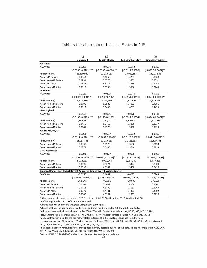
Table A4: Robustness to Included States in NIS

Robustness to Included States in NIS(1) (2) (3) (4)

Uninsured Length of Stay Log Length of Stay Emergency AdmitAll StatesMA*After -0.0231 -0.0504 -0.0012 -0.0202

[-0.0300,-0.0162]*** [-0.0999,-0.0008]** [-0.0111,0.0086] [-0.0397,-0.0007]**N (Nonelderly) 23,860,930 23,913,183 23,913,183 23,913,983Mean MA Before 0.0643 5.4256 1.4267 0.3868Mean Non-MA Before 0.0791 5.0770 1.3552 0.3591Mean MA After 0.0352 5.3717 1.4355 0.4058Mean Non-MA After 0.0817 5.0958 1.3596 0.3745NortheastMA*After -0.0160 -0.0293 -0.0070 -0.0293

[-0.0309,-0.0011]** [-0.2007,0.1421] [-0.0551,0.0411] [-0.0500,-0.0085]**N (Nonelderly) 4,510,280 4,511,992 4,511,992 4,512,094Mean Non-MA Before 0.0790 5.6529 1.4163 0.4281Mean Non-MA After 0.0613 5.6453 1.4203 0.4425New EnglandMA*After -0.0159 -0.0021 0.0170 -0.0411

[-0.0193,-0.0125]*** [-0.1276,0.1233] [-0.0214,0.0554] [-0.0749,-0.0072]**N (Nonelderly) 1,369,181 1,370,420 1,370,420 1,370,438Mean Non-MA Before 0.0450 5.3462 1.3890 0.3337Mean Non-MA After 0.0408 5.3576 1.3840 0.3324All, No ME, VT, CAMA*After -0.0236 -0.0537 -0.0022 -0.0202

[-0.0311,-0.0161]*** [-0.1082,0.0008]* [-0.0129,0.0085] [-0.0417,0.0013]*N (Nonelderly) 21,067,733 21,119,253 21,119,253 21,119,708Mean Non-MA Before 0.0837 5.0926 1.3606 0.3653Mean Non-MA After 0.0871 5.0996 1.3644 0.381325 Most InsuredMA*After -0.0246 -0.0477 0.0056 -0.0066

[-0.0367,-0.0126]*** [-0.0817,-0.0138]*** [-0.0012,0.0124] [-0.0623,0.0491]N (Nonelderly) 8,028,553 8,057,249 8,057,249 8,057,439Mean Non-MA Before 0.0595 4.9274 1.3424 0.3300Mean Non-MA After 0.0638 4.9342 1.3438 0.3426Balanced Panel (Only Hospitals That Appear in Data in Every Possible Quarter)MA*After -0.0273 0.1087 0.0297 0.0244

[-0.0500,-0.0045]** [-0.0872,0.3045] [-0.0038,0.0633]* [-0.0705,0.1193]N (Nonelderly) 768,541 770,696 770,696 770,699Mean MA Before 0.0461 5.4089 1.4104 0.4701Mean Non-MA Before 0.0714 4.6790 1.3037 0.2769Mean MA After 0.0279 5.4701 1.4323 0.4902Mean Non-MA After 0.0800 4.6364 1.2969 0.272095% asymptotic CI clustered by state: *** Significant at .01, ** Significant at .05, * Significant at .10MA*During included but coefficient not reported. All specifications and means weighted using discharge weights.All specifications include hospital fixed effects and time fixed effects for 2004 to 2008, quarterly."All States" sample includes all states in the 2004-2008 NIS. Does not include AL, AK, DE, ID, MS, MT, ND, NM. "New England" sample includes MA, CT, NH, VT, ME, RI. "Northeast" sample includes New England, NY, NJ."25 Most Insured" includes the top half of states in terms of initial levels of insurance from the CPS.

Source: HCUP NIS 2004-2008 authors' calculations. See text for more details.

In decreasing order of insurance, "25 Most Insured" includes: MN, HI, IA, NH, ME, WI, MA, VT, KS, RI, NE, MI, ND (not in NIS), CT, PA, OH, M0, SD, DE (not in NIS), VA, MD, TN, KY, UT."Balanced Panel" only includes states that appear in every possible quarter of the data. These hospitals are in AZ (2), CA, CO (2), GA, MA (2), MD, MN, NC, NE, OH, TN, TX (4), UT, WA (4), WV (2).

52

Table A5: Insurance and Outcomes in Low vs. High Uninsured Hospitals inNIS

Insurance and Outcomes in Low vs. High Uninsured Hospitals in NIS(1) (2) (3) (4)

Uninsured Length of Stay Log Length of Stay Emergency AdmitAll Hospitals (100% of sample, including missing ages)Ma*After -0.0153 -0.0626 0.0006 -0.0367

[-0.0201,-0.0104]*** [-0.1102,-0.0150]** [-0.0090,0.0103] [-0.0585,-0.0149]***N (All Ages) 36,282,073 36,343,449 36,343,449 36,345,238N Hospitals 3,090 3,090 3,090 3,090N Hospitals in MA 48 48 48 48Mean MA Before 0.0409 5.8833 1.5099 0.4789Mean Non-MA Before 0.0543 5.6256 1.4517 0.4291Mean MA After 0.0226 5.7516 1.5084 0.4912Mean Non-MA After 0.0557 5.5819 1.4482 0.4491Only Hospitals that Appear in Data At Least Once Before ReformMa*After -0.0152 -0.0651 -0.0001 -0.0369

[-0.0202,-0.0102]*** [-0.1155,-0.0147]** [-0.0104,0.0102] [-0.0596,-0.0143]***N (All Ages) 30,390,240 30,441,321 30,441,321 30,442,760N Hospitals 2,315 2,315 2,315 2,315N Hospitals in MA 40 40 40 40Mean MA Before 0.0409 5.8833 1.5099 0.4789Mean Non-MA Before 0.0543 5.6256 1.4517 0.4291Mean MA After 0.0230 5.7678 1.5085 0.4856Mean Non-MA After 0.0595 5.5803 1.4460 0.4473Low Uninsured HospitalsMa*After -0.0178 -0.0895 0.0019 -0.0409

[-0.0228,-0.0129]*** [-0.1522,-0.0269]*** [-0.0074,0.0112] [-0.0577,-0.0241]***N (All Ages) 14,407,631 14,426,624 14,426,624 14,427,194N Hospitals 1,157 1,157 1,157 1,157N Hospitals in MA 29 29 29 29Mean MA Before 0.0303 5.8769 1.5058 0.4431Mean Non-MA Before 0.0210 5.6142 1.4487 0.4087Mean MA After 0.0220 5.7938 1.5119 0.4742Mean Non-MA After 0.0295 5.6036 1.4438 0.4306High Uninsured HospitalsMa*After -0.0165 -0.0260 -0.0063 -0.0086

[-0.0246,-0.0085]*** [-0.0782,0.0263] [-0.0151,0.0024] [-0.0312,0.0140]N (All Ages) 15,982,609 16,015,279 16,015,279 16,016,149N Hospitals 1,158 1,158 1,158 1,158N Hospitals in MA 11 11 11 11Mean MA Before 0.0635 5.8969 1.5186 0.5550Mean Non-MA Before 0.0848 5.6360 1.4546 0.4478Mean MA After 0.0314 5.5593 1.4808 0.5769Mean Non-MA After 0.0845 5.5609 1.4478 0.461295% asymptotic CI clustered by state: *** Significant at .01, ** Significant at .05, * Significant at .10MA*During included but coefficient not reported. All specifications and means weighted using discharge weights.All specifications include hospital fixed effects and time fixed effects for 2004 to 2008, quarterly.Low Uninsured Hospitals have less than median uninsurance of 0.0398 before reform.Sample sizes vary across specifications based on availability of dependent variable. Source: HCUP NIS 2004-2008 authors' calculations. See text for more details.53

Table A6: Comparison of Massachusetts Hospital Characteristics in the NISHCUP and Casemix Datasets, AHA Data 2008

Acute Care Hospitals (Casemix

Dataset)

NIS-HCUP Hospitals

[n=64] [n=15]

% Teaching hospitals 21.88 26.67% Community hospitals 98.44 100.00% Short-term hospitals 98.44 100.00% Participant in a hospital network 33.33 35.71% DSH hospitals 28.13 26.67Hospital ownership

Government, Nonfederal: Hospital district or authority 1.56 6.67

% Nongovernment, not-for-profit: Church operated 7.81 0.00% Nongovernment, not-for-profit: Other not-for-

profit 84.38 86.67% Investor-owned (for-profit): Corporation 6.25 6.67

% Government, federal: Veterans Affairs 0.00 0.00

Average total hospital beds 229.78 252.80% Hospitals in each bed size category

6-24 beds 4.69 0.0025-49 beds 9.38 13.3350-99 beds 14.06 20.00

100-199 beds 28.12 26.67200-299 beds 15.62 0.00300-399 beds 12.50 20.00400-499 beds 4.69 6.67

500 or more beds 10.94 13.33Average number of admissions 12,074.88 13,642.67Average inpatient days 61,987.61 68,932.33Average Medicare inpatient discharges 5,231.20 5,761.67Average Medicaid inpatient discharges 2,088.06 2,522.60Average number of mergency outpatient visits 46,983.44 51,384.67Average number of total outpatient visits 304,308.50 327,945.30

Average payroll expenditures 125,000,000 137,000,000Average total expenditures 314,000,000 357,000,000% Net revenue paid on a capitated basis 0.67 0.33% Net revenue paid on a shared risk basis 3.85 2.56

Average number of full-time physicians and dentists 87.86 134.87

Average number of part-time physicians and dentists 23.83 45.07

Hospital Characteristics

Comparison of Massachusetts Hospital Characteristics in the NIS-HCUP and Casemix Dataset

Hospital Bed Size & Admissions

Hospital Expenditures, Payment & Employment

54