THE AMERICAN UNIVERSITY IN CAIRO

SCHOOL OF BUSINESS

The Impact of Exchange Rate Changes on Sectoral Activity:

The Case of Egypt

A Thesis Submitted to the

Economics Department

In partial fulfillment of the requirements for the degree of

Master of Arts in Economics

By: Nada Shokry

Under the supervision of

Dr. Mohammed Bouaddi

May 2017

~ 1 ~

DEDICATION

All the efforts made for this work would not have been possible, first, without Allah’s assistance and reconciliation and secondly, without my husband’s support and understanding as well as my mother’s inspiration and consistent encouragement.

~ 2 ~

ACKNOWLEDGEMENT

I would like to thank my supervisor Dr. Mohamed Bouaddi for his consistent guidance and

help. I would also like to thank Dr. Samer Atallah for getting the best out of my thoughts as I was

choosing my topic in his class: Research Workshop. Finally, I would like to thank the university

and Dr. Ahmed and Ann M. El-Mokadem for believing in me and financially supporting my study

through the Merit, the University and Ahmed and Ann M. El-Mokaddem fellowships without

which it would have been difficult to continue my study at AUC.

~ 3 ~

Abstract

This paper investigates the effect of changes in exchange rate on sectoral production in

Egypt. For this purpose, the study, first, uses a MIDAS regression to compare between the sign

and magnitude of the effect of two exchange rate measures on 22 subsectors and 4 aggregate

sectors’ production in the period between 1982 till 2014. One measure is the monthly deflated

official bilateral exchange rate of EGP against the US dollar and the other is the annual real

effective exchange rate of the EGP. The results show opposite signs and magnitudes when

comparing both measures which is a highly important finding as the effect of exchange rate on

production is a debatable topic where each study shows different results depending on many

aspects including the choice of exchange rate measure. As the real effective exchange rate is more

representative of a currency’s real value, the interpretation of the estimation results is based on

comparing public sectors and subsectors with private ones, export orientation with import

orientation of each sector and sectors being tradable vs. non-tradable. Finally, results show that

most of the low elasticity sectors are public, non-tradable and contribute by only little to GDP,

while most tradable large sectors are highly elastic regardless of import and export shares of sectors.

~ 4 ~

Table of Contents

I. INTRODUCTION...................................................................................... 5

II. LITERATURE REVIEW .........................................................................10

i. Theoretical Research on Exchange Rate’s Effect on Aggregate Output ......................................................................... 10

ii. Empirical Research on the Exchange Rate’s Effect on Aggregate Output: .................................................................... 15

iii. Theoretical and Empirical Research on the Exchange Rate’s Effect on Sectoral Output:.............................................. 19

III. BRIEF OVERVIEW: EGYPT’S SECTORS ...............................................22

IV. DATA ....................................................................................................25

i. Dependent Variables:..................................................................................................................................................... 25

ii. Exchange Rate Variables: .............................................................................................................................................. 26

iii. Other Explanatory Variables (Control Variables): ........................................................................................................ 27

iv. Descriptive Statistics:..................................................................................................................................................... 28

V. METHODOLOGY ..................................................................................31

VI. ESTIMATION RESULTS ........................................................................33

i. Results for the Public Sector .......................................................................................................................................... 33

ii. Results for the Private Sector: ........................................................................................................................................ 35

iii. Results for Aggregated Sectors: ..................................................................................................................................... 36

VII. QUALITATIVE ANALYSIS OF THE RESULTS .................................38

i. Using RER vs. REER ...................................................................................................................................................... 38

ii. Possible Causes of Magnitude Response Differences of Subsectors ............................................................................... 39

iii. Limitations ..................................................................................................................................................................... 45

iv. Recommendations .......................................................................................................................................................... 47

VIII. CONCLUSION ................................................................................48

IX. REFERENCES .......................................................................................50

X. APPENDIX ............................................................................................54

~ 5 ~

List of Tables and Figure

Fig.1.1: Sector’s Value Added Division in Egypt ........................................................................ 22

Fig.1.2: Division of Production by Sector and Subsectors ........................................................... 23

Fig.1.3: Egypt’s Commodity Export and Import Composition in 2015 ....................................... 24

Table 1.1: Descriptive Statistics of the deflated dependent variables (Public Sector) ................. 29

Table 1.2: Descriptive Statistics of the deflated dependent variables (Private Sector) ................ 29

Table 1.3: Descriptive Statistics of the deflated dependent variables (Aggregate Sectors) ......... 30

Table 1.4: Descriptive Statistics of the explanatory variables ...................................................... 30

Table2.1: Estimation Elasticities for the Public Sector ................................................................ 33

Table2.2: Estimation Elasticities for the Private Subsectors: ....................................................... 35

Table2.3: Estimation Elasticities for the Aggregate Sectors’ Value Added: ................................ 36

Table3.1: Elasticities of GDP per Subsector to REER and the subsectors’ share in GDP: .......... 40

Fig.3.2: Import and Export division of Agricultural Products in Egypt (in mio. $) ..................... 42

Fig.3.3: Import and Export Share of Non-Agricultural Products in Egypt (in mio. $) ................. 43

Fig.3.4: Imports and Exports of Commercial Services in Egypt (in mio. $) ................................ 43

Fig.3.5: Transport Imports and Exports of Egypt (in mio. $) ....................................................... 44

Table A: Sectors and Subsectors used in this study ...................................................................... 54

Fig. A: Public and Private Sectors’ Share in Production .............................................................. 54

Table B: R-squared estimation results for both EX measures ...................................................... 55

Table C: Significance of the five Control Variable in both Estimations (REER & RER) ........... 57

~ 6 ~

List of Abbreviations

ARDL: Autoregressive distributed lag model

CBE: Central Bank of Egypt

ECM: Error correction model

EGP: Egyptian Pound

EX: Exchange

IMF: International Monetary Fund

MENA: Middle East and North Africa

MIDAS: Mixed data sampling estimation model

NER: Nominal Exchange Rate

OLS: Ordinary Least Squares

REER: Real Effective Exchange Rate

RER: Real Exchange Rate

~ 7 ~

I. Introduction

The impact of exchange rate on economic activity remains a controversial topic in

empirical literature. According to the traditional Mundell Fleming model, a depreciation (or a

devaluation) of a local currency may stimulate economic activity through the expenditure

switching effect from foreign to domestic goods as their relative prices increase. A significant

supporting evidence for this model is the export and economic growth experience of East Asian

countries maintaining a devalued currency in the last decades. However, empirical literature

provided mixed estimation results when it comes to the effect of devaluation being expansionary

vs. contractionary to economic activity. The huge economic contraction following devaluation in

Latin American economies in the 1990s has led to gained attention to the negative effect of

devaluation in developing countries pointing out to the adverse balance sheet effects. Researchers

refer to many supply and demand side channels in addition to the financial balance sheet channel

as the channels through which devaluation can have a contractionary impact. The thesis project

will discuss in depth the mechanism and different channels mentioned in literature through which

the impact of devaluation on economic activity can differ.

Although many studies examined the impact of exchange rate changes on the aggregate

economic activity, most studies ignored the disaggregated sector and industry-specific dynamics.

The response of sectors and industries should be highly heterogeneous as they differ in main

economic characteristics, such as the degree of trade openness, price elasticity of demand, financial

structure and capital intensity (Hahn, 2007; Karadam, 2014). In this regard, the main aim of the

thesis project is to examine the impact of exchange rate on sectoral and industrial economic activity

in a developing country, namely Egypt from 1982 till 2014.

~ 8 ~

Egypt is an interesting economy to study regarding the impact of exchange rate, especially

after the recent drop in the value of its currency — the Egyptian pound (EGP) — following the

2011 revolution. The uncertain political and economic conditions of Egypt put the understanding

of the impact of exchange rate on the economy on center stage. Egypt has adopted a fixed exchange

rate regime in the 1990s against the US dollar. In the early 2000s, it was allowed to crawl within

two horizontal bands to offset the shortage in foreign exchange. Afterwards, the Central Bank of

Egypt (CBE) floated the EGP in 2003. Consequently, currency depreciated immediately by 30%

and parallel market had to be eliminated temporarily. As a result, the Egyptian pound strengthened

again against the US dollar till it fluctuated around 5.5 L.E. per dollar in 2010 (CBE, 2009/2010

report). However, the situation changed dramatically aftermath of 2011 revolution. Political and

economic instability in Egypt affected the external sector severely, such as tourism revenues,

capital flows and foreign portfolio investments. The resulted deterioration in foreign reserve which

was depleted by around 50% in December 2011 compared to December 2010 and kept declining,

resulted in turn in currency depreciation. Hence, it becomes a vicious circle in which the

depreciation in exchange rate depletes foreign reserves and at the same time, the deterioration in

international reserves pressures the exchange rate (CBE, April 2013 report). Earlier in 2016, EGP

was pegged against the US dollar while parallel market rates increased dramatically till the CBE

finally announced the floatation of the currency in November 2016 depreciating the Egyptian

pound by 50% to secure a 12$ billion IMF loan (The guardian, 3 Nov. 2016).

Finally, the thesis project aims at investigating three key questions. The first question

addresses the impact of exchange rate changes on the different economic sectors’ activities in

Egypt. Identifying those sectors harmed by devaluation and those benefitting provides a more

~ 9 ~

accurate analysis which will help in choosing the right specific industry-targeting policies and in

making the right industry-specific investment decisions. The second addressed question is whether

the public sector is differently affected by exchange rate changes than the private sector’s

production. Depending on which sector’s magnitude of impact is greater, policy should adjust,

either through investment encouragement in one of the sectors or taxes imposition decision. The

last question is whether the measure of exchange rate does make a difference in results. To answer

this question, two different measures of exchange rate are to be used to compare results: bilateral

rate (EGP/$) vs. the effective exchange rate.

~ 10 ~

II. Literature Review

i. Theoretical Research on Exchange Rate’s Effect on Aggregate Output

Dealing with exchange rate is one of the most important issues for policy makers,

especially in developing countries. The reason is that exchange rate is one of the three instruments

used in policies that keep the internal ̶ full employment and price stability ̶ and external balance ̶

current account that realizes savings and investment balance and debt sustainability ̶ of an

economy maintained (Coudert and Couharde, 2009). Two policies help in keeping the balance:

expenditure reducing and expenditure switching mechanisms. Fiscal and monetary policy are the

instruments of the earlier while exchange rate is the instrument used for the latter; the expenditure

switching mechanism (Karadam 2014). Accordingly, exchange rate is said to be misaligned if

there exists a gap (either over or undervaluation) between the real exchange rate of a country and

its equilibrium level, i.e. the level that realizes the internal and external balance (Wong, 2013).

According to the standard Mundell Flemming model - which was widely agreed upon

before the 1970s with no serious controversy – currency depreciation (or devaluation) is

expansionary through its expenditure switching effect from foreign to domestic goods as imports

will relatively be more expensive than domestic production and exports will become more

competitive in international markets with its relatively lower prices. Even stabilization programs

of developing countries monitored by the IMF since the 1950s required the devaluation of the

currency. However, some Latin American countries, especially Brazil, suffered from recessions

after the implementation of adjustment programs which raised the possibility of devaluation being

contractionary especially for developing countries (Karadam, 2014). Some empirical studies

~ 11 ~

pointed out to the negative balance sheet effect in developing and emerging economies due to

financial dollarization through which devaluations were contractionary in those countries.

(Bebeczuk et al., 2006; Blecker and Razmi, 2008). According to Karadam (2014), changes in a

country’s exchange rate affects the economy through three channels: demand side, supply side and

balance sheet effects.

a. Impact of devaluation on aggregate demand:

According to the conventional aggregate demand model, the components of the demand

side are consumption, investment, government spending and net exports. The effect of exchange

rate protrudes on each of the mentioned components in different signs and magnitudes: When it

comes to consumption, the larger the share of traded goods in consumption the more devaluation

reduces real income; the price of traded goods increase followed by an immediate fall in real

household income reducing expenditure. Hence, a devaluation contracts consumption and in turn

aggregate demand if the share of traded goods in consumption is greater than that of the non-traded

goods (Krugman and Taylor, 1963).

Investments in developing countries and most countries except for the US, Germany and

Japan – where most of the world’s capital equipment is produced – require imported capital goods.

When currency depreciates, the price of capital increases and consequently investment decreases

(Branson, 1986). On the other hand, Landon and Smith (2009) argue that the net effect of

depreciation on investment is uncertain as it depends on the degree of substitutability of capital

versus other inputs that are now demanded to produce more exports. If there is a high degree of

substitutability between capital and labor, industries will be more labor intensive rather than capital

intensive which might decrease the cost of production and hence the cost of investment. On the

~ 12 ~

other hand, if the degree of substitutability is low, cost of production will have to increase resulting

in decreased investment. Another channel through which investment can be affected is the

distribution of income that can result from devaluation. Since the owners of export firms benefit

from devaluation and workers are harmed through the reduction in their real income; a

redistribution of income takes place. Since the marginal propensity to save from profits is assumed

to be higher than that of workers, income distribution might increase investment while reducing

consumption (Krugman and Taylor, 1978). Nonetheless, devaluation results in perceived

vulnerability which in turn increases speculation of future devaluation and causes weakened

confidence in the economy (El-Ramly and Abdel-Haleim, 2008). Hence, the impact of exchange

rate on aggregate demand through the investment component is multi-faceted, uncertain and is

relative to the economy’s sectoral structure.

After a devaluation, the value of exportable as well as importable goods increase. If the

government put ad valorem taxes on exports and imports, tax revenue will increase. This means

an income transfer from private to the public sector. Since the marginal propensity to consume

from the government is assumed to be lower than that from the private sector, a reduction in

aggregate demand is induced through increased government revenue yet decreased aggregate

consumption (Krugman and Taylor, 1978).

Finally, the most obvious impact of devaluation on aggregate demand is through increased

international competitiveness of exports and encouraging import substitution, which increases

output. However, counter-inflationary macroeconomic policies result in aggregate demand and

output reduction as well as a deterioration in trade balance. In 1972, the current account of the US,

for instance, experienced the letter “J” after devaluation, decreasing for the short-run due to the

~ 13 ~

counter-inflationary policies then shooting up because of the expansionary effect of devaluation,

thus was labelled the J-curve (El-Ramly and Abdel-Haleim, 2008)

Nonetheless, the net effect on production cannot be solely determined by the demand side.

The magnitude of increase in aggregate demand is to be compared with the magnitude of reduction

in aggregate supply in response to devaluation to decide whether the impact is contractionary or

expansionary

b. Impact of devaluation on aggregate supply:

In macroeconomics, aggregate supply is mainly concerned with inputs of production:

intermediate goods, capital and labor. Since in most developing countries capital and intermediate

goods are mainly imports, a currency devaluation causes an increase in import prices which in turn

increases the cost of production. This increase in import prices is called exchange pass-through -

the percentage increase in import prices as devaluation increases by one percent (Campa and

Goldberg, 2005). Not only does the price of capital increase because of imports, it also increases

because of the increasing cost of working capital. In the case of devaluation, the volume of credit

in the market decreases as interest rates tend to rise due to inflation which negatively affects output

and aggregate supply (Buffie, 1986). Finally, if nominal wages increase with the increase in price

level, i.e. wage indexation, supply is adversely affected by the increase in cost of production

(Edwards, 1986).

Differentiating developing and emerging countries in the economic analysis is due to the

low demand elasticities of exports and imports while mostly having a trade deficit. Large external

debts and high vulnerability are also causes of reduction in expenditure, bankruptcies and

weakened confidence in the economy (El-Ramly and Abdel-Haleim, 2008).

~ 14 ~

c. Impact of devaluation on the balance sheet:

Frankel (2004) argues that the impact of exchange rate is greater on the balance sheet than

the pass-through from increased import prices, especially in the recessions followed by devaluation

in Latin American countries in the 1990s. Balance sheet problems arise when firm’s assets are

denominated in domestic currency while liabilities are denominated in foreign currency (Reinhart

and Calvo, 2000). This concept is called financial dollarization in developing countries where

liabilities are mostly denominated in dollars. Hence, with a sharp devaluation, the risk of

experiencing a sudden stop – large negative reversal of capital inflows – increases (Calvo,

Izquierdo, and Talvi, 2004). The foreign currency debts also make it difficult for monetary and

fiscal policy to deal with the resulted negative effects.

~ 15 ~

ii. Empirical Research on the Exchange Rate’s Effect on Aggregate Output:

Empirical results in literature differ in many aspects. Some studies get contractionary results

for devaluation (Karadam, 2014) on aggregate output, others get the opposite results (e.g. Wong

2013; He 2011) and others find no significant long-run impact of exchange rate . Results depend

mainly on: whether the study is in the long or the short-run, model specification, sample period,

methodology applied, and finally whether the countries under study are developing or developed

(or financially developed or not).

Cooper (1971) and Edwards (1986) agree on devaluation being contractionary in the short-

run in developing countries while having neutral effect in the long-run. Similarly, Kamin and Klau

(1992) find no evidence of a long-run contractionary effect for 27 countries, some of which are

developing and some are not. In contrast, Upadhyaya (1999) found the short-run impact on six

Asian countries to be expansionary while having a neutral and in some cases contractionary effect

in the long-run. Thus, none of these studies provide evidence of expansionary impact in the long-

run. Contrary to these findings, Bahmani-Oskooee et al. (2007) apply panel unit root and panel

cointegration techniques for 42 countries including 18 OECD and 24 non-OECD countries using

four estimation methods. Results show that contractionary impact of devaluation is evident in non-

OECD countries in the long-run, while showing heterogeneous impacts for OECD countries

depending on model specification. Hence, there is no consensus in literature on the sign of the

impact of devaluation on aggregate output on the long-run.

The sample period also affects the results of the empirical studies. Kim and Ying (2007)

compare the effects of currency devaluations in seven East Asian and two Latin American

countries distinguishing pre and post 1997 period due to the financial crisis at that time. Pre-1997

~ 16 ~

period, devaluation was contractionary only for the Latin American countries, while post-1997

devaluation was contractionary for half of the studied East Asian countries as well. Thus, sample

period under study does make a difference in the impact of exchange rate on economic output.

Upadhyaya (1999) examines the effects of devaluation for six Asian countries – India,

Pakistan, Sri Lanka, Malaysia, Thailand and Philippines using a special distributed lag model. No

significant expansionary effect was found for any of the economies neither in the long-run nor in

the short-run. Similarly, Bahmani-Oskooee et al. (2002) studied five East Asian countries using a

cointegration and error correction model, however, results were mixed as depreciation is found to

be contractionary in the long-run for two countries, expansionary for other two and not significant

for the last one. Hence, methodology used makes a difference in the sign and magnitude of the

impact of exchange rate on output.

In most panel-data studies, the impact of exchange rate changes on output is different in

developing countries from developed ones. According to El-Ramly and Abdel-Haleim (2008), the

contractionary effect of devaluation is mostly evident in developing countries because of their low

import and export demand elasticities in response to changes in exchange rate which result in slow

adjustment in current account. Moreover, developing countries are heavily dependent on imports

as intermediate goods, capital goods and raw materials constitute 70% of imports as of 2014 (WITS,

2014). Aghion et al. (2009) studied the impact of exchange rate volatility on productivity growth

in a cross-country panel data using a model that incorporated the level of financial development

and macroeconomic shocks. Results show that real exchange rate volatility can have a significant

impact on productivity growth. However, whether the significant impact is positive or negative

depends mainly on a country's level of financial development. The lower the level of financial

~ 17 ~

development the more negative shocks on volatility are contractionary to productivity growth,

which is more evident in developing countries. Similarly, Sikarwar (2014) argues that emerging

markets firms are significantly exposed to higher exchange rate risk than developed markets.

Hence, the choice of economies under study is significant to the variation in results, especially

developing vs. developed economies.

Finally, the impact of exchange rate on economic activity in Egypt is studied only in a few

studies. Egypt is expected to follow the contractionary impact on developing countries hypothesis

as it is still a developing country. In this regard, El-Ramly and Abdel-Haleim (2008) studied the

relationship between exchange rate changes and output in the Egyptian economy in the period

from 1982 till 2004 using a nonstructural VAR model and annual real effective exchange rate as

the measure of exchange rate while controlling for money supply growth and fiscal policy deficit

as percentage of GDP. The findings of the paper are that devaluation is contractionary for the first

four years, then it starts to be expansionary given that no multiple short-run devaluations happened

in a row postponing the positive impact. Findings of the study also showed the large influence of

real exchange rate changes on output through the econometric results that show real exchange rate

variations explaining as much as 45-68% of the changes in the rate of growth of output. This

suggests that it might not have been wise to allow the floatation of the exchange rate system at the

time of study. However, it is important to note that this study was conducted in 2008 before the

2011 revolution and the series of devaluation that happened afterwards. Results may differ now

and the speed of adjustment of the impact might be longer than four years as found in this study.

Finally, Kandil and Dincer (2008) conducted a comparative study between the impact of changes

in exchange rate on output in Turkey vs. Egypt distinguishing unanticipated – residuals of the

~ 18 ~

model– from anticipated changes in exchange rate – assuming rational expectation– in the period

from 1980 till 2005. Results show that unanticipated depreciation has more pervasive impact than

unanticipated appreciation in Egypt because exports appear to be more inelastic to currency

changes while import prices are highly affected. Hence, due to the limited new studies on Egypt

and to the debatable nature of the research question of the thesis project, there is no consensus on

the empirical results for Egypt which gives room for the thesis project to add significant value in

this regard.

~ 19 ~

iii. Theoretical and Empirical Research on the Exchange Rate’s Effect on Sectoral Output:

The use of the previous aggregate output in the analysis may not be accurate enough to

point out the impact of exchange rate on production as it may be subject to aggregation bias, which

implies that an expansionary effect of exchange rate on one sector may be offset by a negative

effect in another sector while findings may be insignificant or negative at the aggregate level. Even

the aggregate level results depend mainly on the performance of every individual industry which

raises the importance of focusing the analysis to the sectors that contribute most to the aggregate

effect. Sectors are heterogeneous as they differ in many aspects such as the export and import share

in production, production differentiation, price elasticities of demand and supply and exposure to

exchange rate shocks (Hahn, 2007). The magnitude and timing of the impact differs from a sector

to another. Some sectors will be immediately affected and some will experience delayed effect

which will help in detecting the exchange rate effect on inflation at the earliest possible stage.

Sectors with higher import share in inputs, higher degree of product differentiation and

competition reducing factors, will experience a lesser response to exchange rate changes. In

contrast, the higher the export share of a sector, the higher the share of imported competitor goods

and the higher the price elasticity of demand, the higher the magnitude of response of a sector

(Hahn, 2007).

Bahmani-Oskooee and Mirzaie (2000) investigate the impact of exchange rate changes

on the US. production in eight sectors with quarterly data from 1970 till 1994 using a modified

version of the Johansen-Juselius cointegration analysis. In their model, unemployment, oil prices,

government spending and imports were explanatory variables along with the nominal effective

~ 20 ~

exchange rate. The main findings of this paper is that there is no evidence of a long-run relation

between the value of the dollar and sectoral output in the US.

Another wide study was conducted by Hahn (2007) to determine the magnitude & speed

of the impact of exchange rate shocks on activity in all Euro area sectors from 1985 till 2004. Hahn

used a VAR framework as it solves the problem of endogeneity in the variables of the model and

provides the tools to trace out the dynamic responses of the system. The main findings of Hahn

differ from that of Bahmani-Oskoee and Mirzaei (2000) in that its results show industry, added

value in trade and transportation services to be the most sectors affected by an exchange rate shock

while the adjustment in intermediate goods production to be one of the fastest. In the subsectors

of industry, the effect is heterogeneous ranging from zero impact in food production to a very high

response in manufacturing of machinery.

In a doctoral thesis written by (He, 2011) the impact of exchange rate on real output of 24

sectors in 20 OECD countries is examined using ARDL-ECM from 1971 till 2008. According to

the findings of the study, the impact of devaluation is expansionary for two of the three tradable

sectors, namely manufacturing and agriculture, while it is contractionary to half of the non-traded

sectors. As evident from the studies cited above, industry is affected heavily in developed countries

mostly positively by a devaluation as the export share of the production of this sector is higher

than its reliance on imported intermediate inputs. Even firms in Indian industries benefited from

the rupee’s depreciation against the dollar from 2006 till 2011 according to a firm-level analysis

conducted by (Sikarwar, 2014).

Finally, Karadam (2014) examined in his doctoral thesis the impact of real exchange rate

changes on imports, exports, and production of 22 Turkish manufacturing industry’s sub-sectors

~ 21 ~

over the period of 1994 to 2010 taking into consideration the financial dollarization and import

and export share of each sector. Results show that growth in industries is negatively affected by

real depreciations whereas this negative effect is larger for high and medium-high technology

sectors and smaller for export oriented industries. Hence, the result of this study is more similar to

what it is expected to find in the sectors of a developing country, like Egypt. Studies on Egypt or

the Middle East and MENA region are very limited when it comes to industrial analysis of

exchange rate impact which gives room for this thesis project to have a value added in literature.

~ 22 ~

III. Brief Overview: Egypt’s Sectors

The structure of Egypt’s economy is important in the context of this study as results may

differ and have more significant impact depending on several characteristics, such as the size of

each sector in the economy, the export and import orientation of each sector and industry as well

as employment division among the sectors. Unfortunately, detailed data on Egypt for the 22

subsectors examined in this study are not fully and publicly available. However, using the data

already examined in this study and some data on the aggregated division of trade is of some help.

Fig.1.1: Sector’s Value Added Division in Egypt

Data Source: The World Bank

According to Fig.1.1, the division of the sectors’ value added in GDP in 2015 did not differ

greatly from that in 1980. The largest sector as percentage of GDP was and still is the services

sector and the lowest is agriculture. This suggests that a significant large coefficient in the results

for the effect of exchange rate on the services sector means higher effect on the whole economy,

an effect that accounts for around 50%. All subsectors data in this study can fit under these four

categories – except for petroleum excluding petroleum products as it is a separate entity – as shown

in Table A in the appendix.

Services

48%

Industry

32%

Agricuture

20%

Sectors' Value Added in 1982

Services

53%Industry

36%

Agricuture

11%

Sectors' Value Added in 2015

~ 23 ~

Fig.1.2: Division of Production by Sector and Subsectors

Source: Ministry of Planning of Egypt (data used for estimation)

As is shown in Fig1.2, the subsectors petroleum, industry and mining and the money

market are the largest subsectors in the public sector and are larger than those in the private sector

accounting for around 72% of the public sector’s production. The GDP of the Suez Canal is the

fourth largest, however, accounting for only 9% of the public sector’s GDP. Thus, the regression

results of these four subsectors are the most important results for the public sector. On the other

hand, the three largest subsectors in the private sector are industry & mining, agriculture and trade

accounting together for 61% of the total GDP of the private sector. Housing and construction

subsectors are significantly larger in the private sector than they are in the public sector. After all,

the share of the private sector as a whole accounts for almost 75% of the total production –

excluding insurance services - while the public sector accounts only for 25% (Fig. A in the

appendix). Accordingly, the regression results for these five subsectors are the most import results

for the private sector.

Agricultur

e

0%

Industy &

mining

27%

Petroleum

Pr.

33%

Electricity

7%

Constructi

on

2%

Transport.

& Storage

4%

Telecom.

2%

Suez

Canal

9%

Trade

4%

Money

Market

12%

Hotels &

Restaurant

s

0%

Housing

& real

estate

0%

P U B LI C S E C T O R

P R O D UC T I O N

I N 2 0 1 5

Agricultur

e

20%

Industy &

mining

20%

Petroleum

Pr.

5%Electricity

0%Construction

8%

Transporta

tion &

Storage

6%

Telecommun

ication

2%

Trade

21%

Money

Market

3%

Hotels &

restaurants

3%

Housing &

real estate

12%

P R I V A TE S E C T O R

P R O D UC T I O N

I N 2 0 1 5

~ 24 ~

After visualizing the division of sectors and subsectors in the economy’s structure, it is

then important to examine the export and import composition of trade in Egypt. Unfortunately,

data for subsector composition is not readily available unlike the aggregate structure or the specific

products division, such as in Fig.1.3:

Fig.1.3: Egypt’s Commodity Export and Import Composition in 2015

Data Source: World Trade Organization

The industry and mining sector encompasses manufactures as well as fuels and mining

which account together for nearly 75% of Egypt’s exports, while agricultural products account for

the rest of the commodity exports. Similarly, 77% of Egypt’s imports are industrial products as

opposed to 23% agricultural products. Despite the similar aggregate structure of Egypt’s imports

and exports, they differ in products and in size. As of 2015, the size of exports is $19 051 million

as opposed to $65 044 million as the size of imports resulting in a deficit of $46 million, which

account for a negative 14% of GDP. This insight gives rise to negative expectations of the effect

of devaluation on sectoral activity because the size of imports is higher in all sectors of commodity

trade.

Agricultura

l products

26%

Fuels and

mining

products

25%

Manufactures

49%

B R E A KD O W N O F E GY PT ' S

TO TA L C O M M O D I T Y

E X PO RT I N 2 0 1 5

Agricultura

l products

23%

Fuels and

mining

products

21%

Manufactur

es

56%

B R E A KD O W N O F E GY PT ' S

TO TA L C O MMO D I T Y

I MPO RT I N 2 0 1 5

~ 25 ~

IV. Data

In this study, there are two estimations with 26 dependent variables, five macroeconomic

control variables and two explanatory variables- one for each estimation. Some data for Egypt are

challenging to find which made this study a multi-sourced one. The study is conducted over the

period from 1982 till 2014.

i. Dependent Variables:

Sectoral output represented in the dependent variables are divided into public and private

for each sector, except for the Suez Canal public sector. The sectors included in the study are:

agriculture, industry and mining, petroleum products, electricity, construction, transportation and

storage services, telecommunication services, trade, money market, hotels and restaurants and

finally housing and real estate property. Hotels and restaurants can be a proxy of tourism revenue

as there was no indicator for tourism to cover this sample period. The data for GDP per sector in

EGP are current, annual and are retrieved from the website of the Ministry of Planning of Egypt

(MoP). In addition to the data divided into public and private sector data, aggregated value added

data for agriculture, industry, manufacturing and services are also included. These aggregated data

are retrieved from the World Bank country indicators (World Bank). Using the GDP deflator, these

data will be real instead of nominal.

~ 26 ~

ii. Exchange Rate Variables:

A comparison will be conducted between using monthly official nominal exchange rate

manually deflated by the ratio of GDP deflator of Egypt and that of the USA, and annual real

effective exchange rate to test if results will differ as there was no consensus in literature as to

which measure is better. The advantage of the effective exchange rate is that it is a multilateral

measure of the EGP against 67 countries which considers the international trade of Egypt with

other countries other than the US or whose exchange rates are not affected by the US dollar. It is

a more accurate measure of the real value of the Egyptian currency against the trading partners

which gives it a strong explanatory power. On the other hand, monthly frequency gives room for

examining the difference the monthly volatility can do to results as the number of observations is

12 times greater. For the sample period 1982 to 1998, the source for the monthly official exchange

rate is the official website of Carmen Reinhardt, where she collected and measured official and

parallel market exchange rates for more than 100 countries from 1946 till 1998 (Reinhardt). This

is the only online source for monthly official exchange rate for the specified period. Beginning

from 1999 till 2014 monthly official exchange rate is retrieved from Citadel Capital at the

American University in Cairo. Annual real effective exchange rate of the EGP against the

currencies of 67 countries is retrieved from Darvas (2012) who constructed a database for

calculating the nominal and real effective exchange rates for 178 countries and is being updated

continuously.

~ 27 ~

iii. Other Explanatory Variables (Control Variables):

In vast literature, macroeconomic variables are being controlled for when investigating the

relationship between exchange rate and sectoral output. In this study government spending, GDP

per capita, oil prices, inflation and real interest rates are controlled for. All these annual indicators

are retrieved from the World Development indicators of the World Bank (World Bank), except for

oil prices which is on monthly frequency and is retrieved from the US. Energy Information Agency

(EIA). All variables are deflated by the annual GDP deflator of Egypt.

~ 28 ~

iv. Descriptive Statistics:

The following four tables show the statistics of the key variables in this study, namely all

dependent variables used, the two explanatory variables and excluding control variables. Table 1.1,

Table1.2 and Table 1.3 show the statistics of 33 observations from 1982 till 2014 for the real GDP

per subsector in the public sector, the private sector and for aggregate value added in sectors

respectively. Finally, Table 1.4 shows the statistics of 36 observations from 1980 till 2015 for the

annual real effective exchange rate (REER) and the statistics of 525 monthly observations from

January 1974 till October 2016 for the monthly official nominal exchange rate (NER). For

estimations, only observations from 1982-2014 were used, which means 33 observations for

annual data and 396 observations for monthly data (RER and ROIL, a control variable). Moreover,

all variables used in the estimations are either real or deflated including the bilateral exchange rate.

Finally, all dependent variables are measured in current million EGP.

As is evident in Table 1.1, petroleum and its products have the highest mean, highest

maximum and highest standard deviation among public subsectors which is due to the volatility

of their global market and the ongoing technological advances and new sight discoveries.

Agriculture has the lowest mean and minimum, while industry has the highest minimum, which

shows the decreasing nationalization of lands in the public sector and the involvement of the public

sector to provide mining and industrial products for subsistence. Public hotels and restaurants do

not seem to be highly volatile as it recorded the lowest standard deviation among the subsectors

of the public sector.

~ 29 ~

Table 1.1: Descriptive Statistics of the deflated dependent variables (Public Sector)

Variable Public Sector Mean Maximum Minimum Std. Dev.

y1 Agriculture 21 240 2 41

y2 Industry & mining 2616 12920 171 3204

y3 Petroleum & its prod. 5510 23223 64 6295

y4 Electricity 1003 5674 17 1223

y5 Construction 650 7239 36 1246

y6 Transport. & Storage 740 3923 48 793

y7 Telecom. 685 4326 25 859

y8 Suez Canal 1715 7470 30 1728

y9 Trade 457 2287 55 512

y10 Money Market 2157 13876 63 2788

y11 & Restaurants Hotels 30 97 5 21

y12 Housing & Real Estate 36 259 3 48 Source: Author’s Calculations

In contrast to the public sector, agriculture shows the highest mean and minimum in the

private sector, petroleum and its products do not account for the highest maximum among

subsectors but rather industry & mining with the highest standard deviation. It is clear from the

table that the statistics in all private subsectors are higher than those of the public sector except for

petroleum and its products. Hence, the government plays its role as the corrector of market

shortfalls.

Table 1.2: Descriptive Statistics of the deflated dependent variables (Private Sector)

Variable Private Sector Mean Maximum Minimum Std. Dev.

y13 Agriculture 10323 60504 351 12314

y14 Industry & mining 10014 60976 132 12615

y15 Petroleum & its prod. 1591 8685 19 2102

y16 Construction 2636 10164 68 2987

y17 Transport. & Storage 2599 15958 54 3304

y18 Telecommunication 620 2455 0 838

y19 Trade 8988 55175 275 11241

y20 Money Market 1151 6645 20 1467

y21 & Restaurants Hotels 1599 5565 22 1676

y22 Housing & Real Estate 2267 15706 50 3938 Source: Author’s Calculations

~ 30 ~

Table 1.3 shows that the highest statistics belong to the value added of the services sector,

while the lowest belong to the agricultural sector. These statistics will be affirmed by the figure

the next section ‘Data Characteristics’.

Table 1.3: Descriptive Statistics of the deflated dependent variables (Aggregate Sectors)

Variable Aggregates Mean Maximum Minimum Std. Dev.

y23 Services 31570 168148 831 37723

y24 Manufacturing 11183 63480 261 13687

y25 Industry 22475 100420 429 25892

y26 Agriculture 9327 56250 325 11362 Source: Author’s Calculations

The statistics of the two exchange rate measures in Table 1.4 are not to be compared with

each other as the values of both are calculated in an entirely different way. However, inferences

about the dates of the maximum and minimum values can be compared: The maximum of REER

occurred in 1988, while the minimum occurred in 2004. On the other hand, the maximum of NER

occurred in October 2016 while the minimum occurred in January 1974 and remained the same

till November 1978. It is important to note that the exchange rate regime was pegged at different

times on this sample period, while the real effective exchange rate is a calculation that cannot be

fixed.

Table 1.4: Descriptive Statistics of the explanatory variables

Variable Mean Maximum Minimum Std. Dev.

REER 147.2 281.7 84.2 51.5

monthly NER (before deflating) 3.3 8.9 0.4 2.5

Source: Author’s calculations

~ 31 ~

V. Methodology

Two estimations were run by e-views software. One estimation uses annual real effective

exchange rate as the measure of exchange rate, while the other uses monthly bilateral deflated

exchange rate. After deflating all nominal variables by the GDP deflator of Egypt and the nominal

exchange rate by the ratio of GDP deflator of Egypt over that of the US, the first step was to check

the stationarity of the variables using unit root tests. All variables showed to be stationary, where

the unit root hypothesis was rejected for all variables except for government expenditure, a control

variable. However, after smoothing the government expenditure indicator, the variable became

stationary. This test is important in determining which method to proceed with. The study would

have utilized either the Vector Autoregressive Model (VAR) methodology or the Autoregressive

Distributed Lag (ARDL) bounds test to co-integration and error correction model (ECM) initiated

by Pesaran et al.(1999) – had not the unit root test been rejected. These tests were then eliminated

and the conventional OLS estimation model was used for this study.

Consequently, all variables are I(0) and the OLS equation is constructed as follows:

yit

= c + β1lnREX

t +β

2lnGDPC

t + β

3lnGOV

t+ β

4lnINT

t+ β

5lnOILP

t+ β

6lnINFL

t+ε

t

• where REXt: denotes the exchange rate measure at time t (once as the annual real effective

exchange rate and once as the deflated official bilateral exchange rate)

• GDPCt: deflated GDP per capita

• GOVt: deflated and smoothed government spending

• INTt: deflated interest rate

• OILPt: international real oil prices

• INFLt: inflation rate

• yit: deflated sector GDP

~ 32 ~

The logarithm (ln) is used to be able to make an inference about the β coefficients as they

represent the elasticity of the y variables to changes in the accompanied explanatory variables.

Having two variables in monthly frequency – namely, the bilateral exchange rates and the real oil

prices, makes it necessary to use the Mixed-data sampling MIDAS estimation method. It is a

method of estimation from models where the dependent variable is recorded at a lower frequency

than one or more of the independent variables. Contrary to the traditional approach where data

were aggregated in the lower frequency, MIDAS uses information from every observation in the

higher frequency space without aggregation (IHS eviews9) so that the volatility of the higher

frequency would be benefited from.

~ 33 ~

VI. Estimation Results

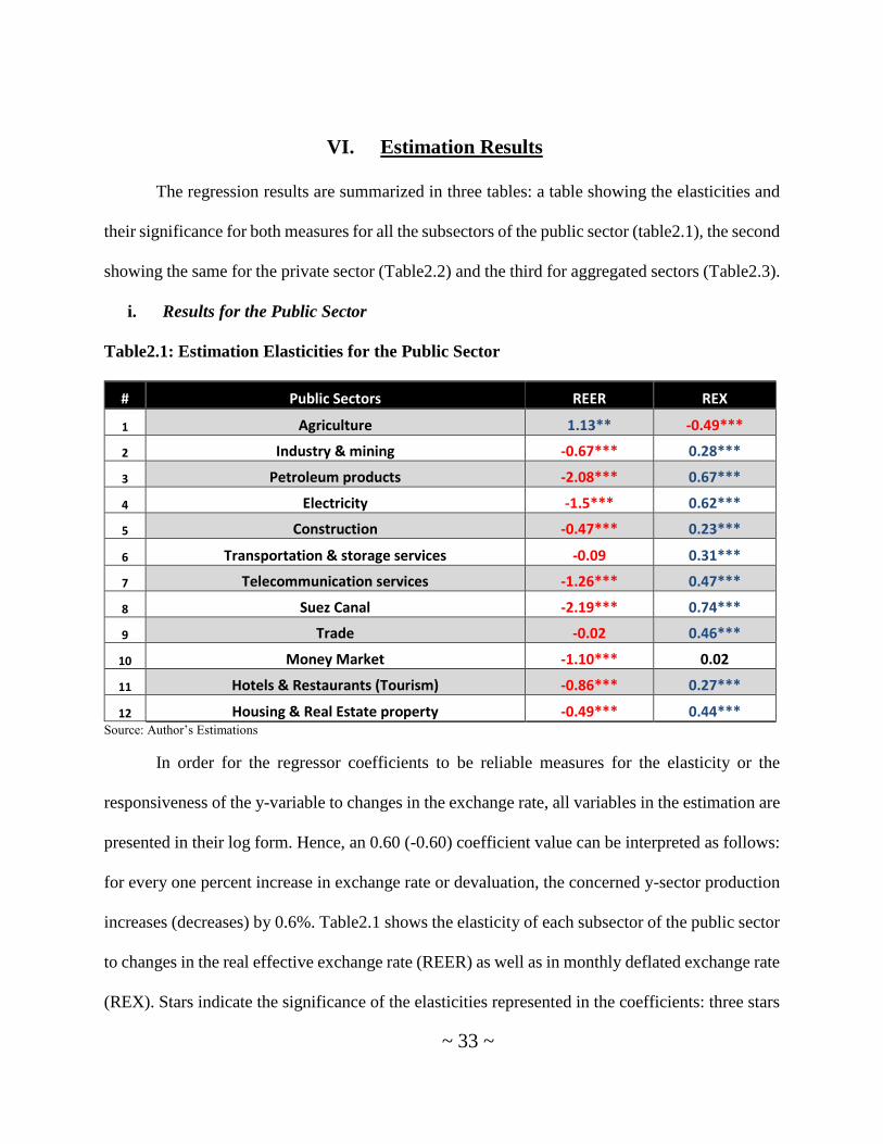
The regression results are summarized in three tables: a table showing the elasticities and

their significance for both measures for all the subsectors of the public sector (table2.1), the second

showing the same for the private sector (Table2.2) and the third for aggregated sectors (Table2.3).

i. Results for the Public Sector

Table2.1: Estimation Elasticities for the Public Sector

# Public Sectors REER REX

1 Agriculture 1.13** -0.49***

2 Industry & mining -0.67*** 0.28***

3 Petroleum products -2.08*** 0.67***

4 Electricity -1.5*** 0.62***

5 Construction -0.47*** 0.23***

6 Transportation & storage services -0.09 0.31***

7 Telecommunication services -1.26*** 0.47***

8 Suez Canal -2.19*** 0.74***

9 Trade -0.02 0.46***

10 Money Market -1.10*** 0.02

11 Hotels & Restaurants (Tourism) -0.86*** 0.27***

12 Housing & Real Estate property -0.49*** 0.44*** Source: Author’s Estimations

In order for the regressor coefficients to be reliable measures for the elasticity or the

responsiveness of the y-variable to changes in the exchange rate, all variables in the estimation are

presented in their log form. Hence, an 0.60 (-0.60) coefficient value can be interpreted as follows:

for every one percent increase in exchange rate or devaluation, the concerned y-sector production

increases (decreases) by 0.6%. Table2.1 shows the elasticity of each subsector of the public sector

to changes in the real effective exchange rate (REER) as well as in monthly deflated exchange rate

(REX). Stars indicate the significance of the elasticities represented in the coefficients: three stars

~ 34 ~

means significant at 1%, two stars significant at 5% and one star significant at 10%. All negative

values indicating a negative relationship between exchange rate and sector performance – which

means devaluation having a negative effect on subsectors – are presented in red and the positive

values in blue. Most of the estimations using both measures showed R-squared to be between 0.80

and 0.95 (Table B in appendix) which shows the strength of the regression equation and that the

model explains from 80% to 90% of the variability in sector production.

Many inferences can be drawn from this table. First, the results of the regression using

REER are the opposite of those of the regression using RER in all subsectors. Secondly, when

analyzing the REER results, it is observable that all elasticities are negative, except for agriculture,

which accounts for less than 0.5% of the public-sector production which can be ignored. In

addition, all elasticities are significant at 1%, except for agriculture, which is significant at 5% as

well as the elasticities of transportation and storage, and trade which are insignificant.

Interestingly, the five largest subsectors in the public sector - namely industry and mining,

petroleum and its products, the money market, Suez Canal and finally electricity generation – show

the highest coefficients or elasticities exceeding 100% to changes in REER. For instance, the

petroleum and its products and Suez Canal respond with a 200% decrease for every 100% increase

in the REER measure. On the other hand, housing and real estate property as well as construction

are showing the lowest elasticities, while both subsectors combined do not account for more than

2.5% of the public sector’s production. Hence, it can be concluded that the public sector as a whole

is significantly vulnerable to currency depreciation or REER increase.

~ 35 ~

ii. Results for the Private Sector:

Table2.2: Estimation Elasticities for the Private Subsectors:

# Private Sector REER REX

13 Agriculture -1.10*** 0.44***

14 Industry & mining -1.53*** 0.65***

15 petroleum products -1.71*** 0.61***

16 Construction -1.28*** 0.51***

17 Transportation & storage services -1.34*** 0.54***

18 Telecommunication services -3.79*** 1.50***

19 Trade -1.12*** 0.46***

20 Money Market -2.08*** 0.54***

21 Hotels & Restaurants (Tourism) -0.68** 0.78***

22 Housing & Real Estate property -1.10*** 0.27*** Source: Author’s estimations

Table2.2 shows again the contradicting results of estimations when using REER and REX

as all REER estimations are highly negative while REX estimations are positive. All coefficients

are significant at 1%, except for hotels and restaurants which is significant at 5%. Again, Table B

in the appendix shows R-squared for all estimations to be in the range from 0.85 to 0.97 which

shows a model with high explanatory power.

Compared to the public sector’s results, the private sector shows higher elasticities for all

subsectors to the extent that all of them are higher than 1, especially the telecommunications

services with an elasticity of 3.79 despite being the smallest subsector in the private sector.

Similarly, money market accounts only for 3% of the private sector’s production and its elasticity

exceeds 2 being highly elastic. In contrast, the largest subsectors – agriculture, industry and mining

and trade - do not show the highest elasticities as it did in the public sector yet are still high. The

~ 36 ~

only subsector with an elasticity lower than 1 is hotels and restaurants which accounts for only 3%

of the private sector’s production.

iii. Results for Aggregated Sectors:

Table2.3: Estimation Elasticities for the Aggregate Sectors’ Value Added:

# Aggregate Value Added REER REX

23 Agriculture -1.22*** 0.25***

24 Industry -1.35*** 0.27***

25 Manufacturing -1.50*** 0.27***

26 Services -1.09*** 0.23*** Source: Author’s Estimations

Table2.3 shows the elasticities of the aggregated sectors’ value added using both REER

and REX. All elasticities for the REER are negative while for the REX are all positive and are all

significant at 1%. Corresponding elasticities of the sectors using REER are all greater than 1

showing high elasticity while all elasticities using the REX are all less than 0.5 showing low

elasticities. As discussed in the data characteristics using Fig.1, the services sector is the greatest

sector accounting for 50% of Egypt’s value added, while agriculture is the smallest accounting for

11% of the total value added. Hence, these results suggest that the total value added is highly

elastic and responsive to changes in the real effective exchange rate.

Conclusion: Egypt’s sectors’ GDP and value added are all highly elastic to and negatively

affected by currency depreciation using REER measure. There is no subsector in the 22 private

and public subsectors is not negatively related to devaluation using REER, except for public

agriculture which contributes with less than 0.5% to the public sector’s GDP. On the other hand,

~ 37 ~

subsectors and aggregated sectors are all positively affected by currency depreciation using the

deflated monthly EX rate and are relatively less elastic with most of the elasticities being less than

1.00. Finally, Table C in the appendix shows the significance of each control variable to changes

in the subsectors’ and sectors’ GDP for both estimations. GDP per capita shows the highest

significance for subsectors for both estimations followed by the government expenditure.

Generally, control variables are more frequently significant in the REER estimations than in the

RER estimations despite being similar.

~ 38 ~

VII. Brief Qualitative Analysis of the Results

i. Using RER vs. REER

Most literature use only one measure to examine the effect of exchange rate on economic

activity, either the effective exchange rate or the bilateral exchange rate which according to the

above results might result in two studies showing opposite results for the same economy. Real

effective exchange rate is often more interesting for economists to study as it is considered as the

average of all the bilateral exchange rates of the trading partners of the economy under study,

weighted by the trade shares of each partner after adjusting for inflation differentials. Therefore,

the results of the regression using REER should have more explanatory power when it comes to

the sectoral activity and accordingly the elasticities estimated using REER are the ones to be

studied further.

RER showing opposite results from REER estimations is an interesting finding as it

suggests that using RER in evaluating the economy’s performance after a devaluation is

misleading. While the economy is harmed by devaluation as the REER estimations show, the RER

shows consistent positive results. The Implication of such a discrepancy would be making wrong

or harmful policies regarding the currency’s value if the regime is pegged or is floating yet

managed which are both the cases in Egypt for the past 30 years.

~ 39 ~

ii. Possible Causes of Magnitude Response Differences of Subsectors

As discussed in literature, there are several factors that could affect the sign and magnitude

of the sector’s production response to changes in exchange rate such as the export and import share

in production, production differentiation, price elasticities of demand and supply and exposure to

exchange rate shocks. Sectors with higher import share in inputs, higher degree of product

differentiation and competition reducing factors, will experience a lesser response to exchange rate

changes. In contrast, the higher the export share of a sector, the higher the share of imported

competitor goods and the higher the price elasticity of demand, the higher the magnitude of

response of a sector (Hahn, 2007). Unfortunately, data on Egypt’s sectors is too scarce to be able

to compare literature with estimation results for Egypt. However, with the data available and the

examination of other factors a brief explanation attempt for the results will be developed in this

section.

Table3.1 categorizes the subsectors according to their magnitude of response or elasticity

to changes in REER and the subsectors’ share in GDP to give an insight of how much the economy

can be affected by the subsector’s response to devaluation. All the subsectors in the <0.5 elasticity

category, do not exceed 1% of their share in GDP while almost all of the subsectors contributing

by more than 5% to the economy’s GDP are in the >1.0 elasticity category, except for public

industry and mining which accounts for approximately 5% and is in the middle category of >0.5

& <1.0 elasticity. On the other hand, those subsectors that have more than 2.0 elasticity such as

the Suez Canal, private telecommunication services, and the private money market contribute each

with less than 2%. Hence, those subsectors contributing most to the aggregate GDP are highly

elastic to REER changes with an elasticity higher than 1.00.

~ 40 ~

Table3.1: Elasticities of GDP per Subsector to REER and the subsectors’ share in GDP:

Elasticity < 0.5

Share in

GDP (%) > 0.5 & < 1.0

Share in

GDP (%) > 1.0

Share in

GDP (%)

Public Construction 0.47

Public Industry &

Mining 5.19 Public Agriculture 0.01

Public Transport. &

Storage (insignificant) 0.81

Public Hotels &

Restaurants 0.02

Public Petroleum &

its Prods. 6.46

Public Trade(insignificant) 0.71

Private Hotels &

Restaurants 1.81 Public Electricity 1.37

Public Housing & R.E. 0.01

Public Telecom.

Services 0.41

Suez Canal (> 2.0) 1.68

Public Money Mrkt 2.33

Private Agriculture 11.17

Private Industry &

mining 11.4

Private Petroleum

& its Prod. 3

Private

Construction 4.33

Private

Transportation &

Storage 3.48

Private Telecom.

(> 3.0) 0.96

Private Trade 12.2

Private Money Mkt

(> 2.0) 1.52

Private Housing &

R.E. 6.75

Source: Author’s Estimations

a. Public vs. Private Subsectors

It is worth noting that all the subsectors in the low elasticity category in Table1.3 are public

subsectors and all the private sectors are listed under the high elasticity category. Moreover, the

highest public subsector contributors to GDP are listed in the highly elastic category such as the

public subsector of petroleum and its products and public mining and industry. Therefore, it can

be concluded that public subsectors are more likely to be less responsive to changes in REER than

are private subsectors, except for mining and industry, and petroleum products. A possible

~ 41 ~

explanation could be that public sectors produce what the market fails to produce so the amount

of production is not to be affected by market prices as produced amounts should meet certain needs

and hence are inflexible to price changes. However, the public as well as private subsector

petroleum and its products including natural gas being highly elastic and negatively signed is

against the common belief in literature and economic concepts as Egypt’s exports mainly depend

on them and on mining which should suggest a devaluation to positively affect the production and

not vice versa.

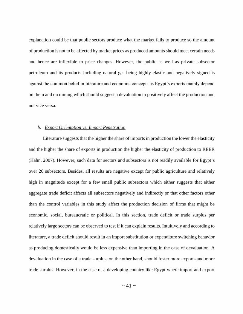
b. Export Orientation vs. Import Penetration

Literature suggests that the higher the share of imports in production the lower the elasticity

and the higher the share of exports in production the higher the elasticity of production to REER

(Hahn, 2007). However, such data for sectors and subsectors is not readily available for Egypt’s

over 20 subsectors. Besides, all results are negative except for public agriculture and relatively

high in magnitude except for a few small public subsectors which either suggests that either

aggregate trade deficit affects all subsectors negatively and indirectly or that other factors other

than the control variables in this study affect the production decision of firms that might be

economic, social, bureaucratic or political. In this section, trade deficit or trade surplus per

relatively large sectors can be observed to test if it can explain results. Intuitively and according to

literature, a trade deficit should result in an import substitution or expenditure switching behavior

as producing domestically would be less expensive than importing in the case of devaluation. A

devaluation in the case of a trade surplus, on the other hand, should foster more exports and more

trade surplus. However, in the case of a developing country like Egypt where import and export

~ 42 ~

elasticities are low, debts are increasing and the economy becoming more vulnerable, the general

contractionary effect on sectors is expected.

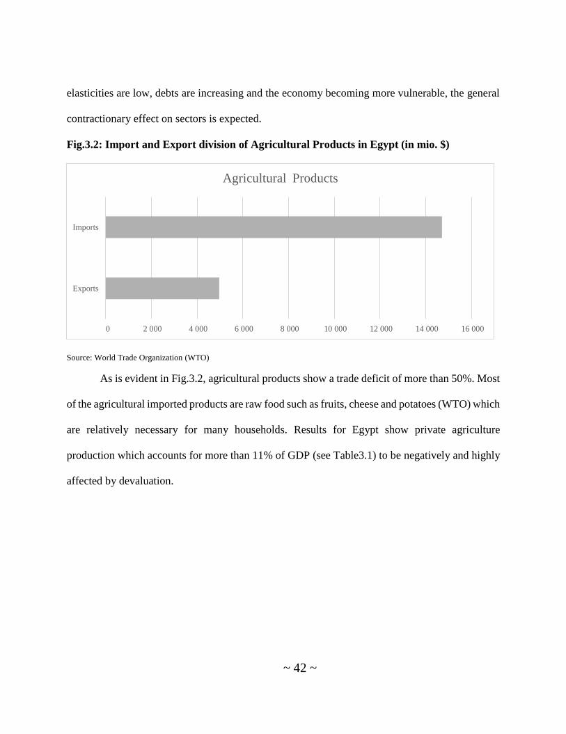
Fig.3.2: Import and Export division of Agricultural Products in Egypt (in mio. $)

Source: World Trade Organization (WTO)

As is evident in Fig.3.2, agricultural products show a trade deficit of more than 50%. Most

of the agricultural imported products are raw food such as fruits, cheese and potatoes (WTO) which

are relatively necessary for many households. Results for Egypt show private agriculture

production which accounts for more than 11% of GDP (see Table3.1) to be negatively and highly

affected by devaluation.

0 2 000 4 000 6 000 8 000 10 000 12 000 14 000 16 000

Exports

Imports

Agricultural Products

~ 43 ~

Fig.3.3: Import and Export Share of Non-Agricultural Products in Egypt (in mio. $)

Source: World Trade Organization (WTO)

Non-Agricultural Products include petroleum oil crude and other than crude, medicaments

and other metal products. Again, a trade deficit of more than 50% is to be observed even though

Egypt’s largest exports are petroleum and natural gas. Public and private production combined of

petroleum products alone contribute by nearly 10% of GDP (see Table3.1) and are negatively

affected and highly elastic to currency depreciation.

Fig.3.4: Imports and Exports of Commercial Services in Egypt (in mio. $)

Source: World Trade Organization (WTO)

0 10 000 20 000 30 000 40 000 50 000 60 000

Exports

Imports

Non-Agriclutral Products

15 500 16 000 16 500 17 000 17 500 18 000 18 500

1

2

Commercial Services

~ 44 ~

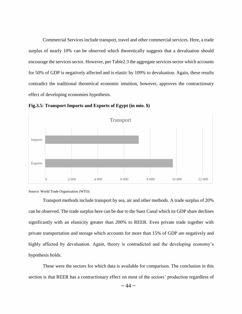
Commercial Services include transport, travel and other commercial services. Here, a trade

surplus of nearly 10% can be observed which theoretically suggests that a devaluation should

encourage the services sector. However, per Table2.3 the aggregate services sector which accounts

for 50% of GDP is negatively affected and is elastic by 109% to devaluation. Again, these results

contradict the traditional theoretical economic intuition, however, approves the contractionary

effect of developing economies hypothesis.

Fig.3.5: Transport Imports and Exports of Egypt (in mio. $)

Source: World Trade Organization (WTO)

Transport methods include transport by sea, air and other methods. A trade surplus of 20%

can be observed. The trade surplus here can be due to the Suez Canal which its GDP share declines

significantly with an elasticity greater than 200% to REER. Even private trade together with

private transportation and storage which accounts for more than 15% of GDP are negatively and

highly affected by devaluation. Again, theory is contradicted and the developing economy’s

hypothesis holds.

These were the sectors for which data is available for comparison. The conclusion in this

section is that REER has a contractionary effect on most of the sectors’ production regardless of

0 2 000 4 000 6 000 8 000 10 000 12 000

Exports

Imports

Transport

~ 45 ~

the import penetration or export orientation of the sector. The aggregate trade deficit is affecting

all sectors negatively as Egypt is following the overall contractionary effect hypothesis of

developing countries.

c. Tradable vs. Non-Tradable Subsectors:

Another theoretical explanation for observed differences in magnitude and sign of the

subsectors to changes in REER could be the distinction between tradable and non-tradable sectors.

Intuitively, tradable sectors should be more affected in magnitude by REER than are non-tradable

sectors as production decision is not affected directly by changes in REER and prices. Tradable

sectors are industries that produce goods and provide services that are or can be traded

internationally, such as the manufacturing sector, while non-tradable sectors are those that provide

services that can only be used domestically and using only domestic workforce, such as

construction, education, health, housing services…etc.

In the case of Egypt according to Table3.2, most of the low elasticity sectors are public,

non-tradable and contribute by only little to GDP, such as public housing and real estate, public

construction and public hotels and restaurants. On the other hand, however, there are other many

private non-tradable subsectors in the highly elastic category as well, such as private housing and

real estate, private construction and private and public telecommunication. Hence, the distinction

in tradable and non-tradable sectors as a possible differentiation point between highly elastic and

relatively more inelastic subsectors’ production to changes in REER is not strong factor.

~ 46 ~

iii. Limitations

There are several limitations to this study. First, this study does not cover the period after

2014 which witnessed a sudden great devaluation after floatation. Even though this study is

focused on historical time series which gives insight to the consequences that can happen with the

current devaluation, including the time of great devaluation might influence results. Moreover, as

the exchange rate system was pegged for more than 20 years at the beginning of the studied sample

period, black market rates could have been more indicative of the changes in the value of the

currency. However, black market rates for this whole sample period was lacking for Egypt.

Another limitation which is not high in importance, the bilateral exchange rate was deflated

by the GDP deflator over the GDP deflator of the US and sectors’ production were deflated by the

GDP deflator, while it could have been more accurate to use the CPI deflator instead of the GDP

deflator and CPI deflator per sector instead of an aggregate one. However, such data is not readily

available for Egypt for this sample period.

Finally, the import and export share of production as in raw materials is not readily

available for Egypt which could have given more insight and explanation to estimation results.

~ 47 ~

iv. Recommendations

This study is a gateway to further deeper analysis of each subsector and to other influencing

factors other than those mentioned in this study. A deeper analysis of each sector’s characteristics

and economic background can be further developed. Degree of product differentiation, export and

import share of each sector and subsector, price elasticity of demand as well as competition factors

are all characteristics that can be quantitatively considered while running estimations. However,

data will have to be available or accommodable for Egypt. Another important extension to this

study would be to make the same analysis to the recent floatation and sharp devaluation period

starting in 2016, however, higher frequency data will have to be available to have a sufficient

sample period. Due to the lengthy period of pegged system in Egypt, black market rates could be

compared to the REER instead of the official exchange rate. Moreover, comparing Egypt’s results

with results of another developing country as well as another developed one or constructing a panel

data model could give more insight to Egypt’s situation. Finally, the effect of this study’s results

on inflation or pass-through can also be further studied.

~ 48 ~

VIII. Conclusion

This study has provided many valuable findings and a basis for further more focused research.

The first finding is that the choice of exchange rate measure is an immediate influence in the sign

and magnitude of results; using the monthly bilateral deflated exchange rate of the Egyptian pound

vs. the US dollar provided totally opposite results to the annual real effective exchange rate results.

As REER should have more explanatory power as it is by nature calculated in a way to be more

comprehensive and to be more representative of the value of the Egyptian currency and all of the

currencies of Egypt’s trade partners, REER results are the one to be relied on. REER results

showed negative elasticities for all subsectors, except for public agriculture, while RER results

showed positive elasticities for all subsectors. At the same time, most results are highly significant

for both measures. Hence, devaluation measured by REER is contractionary to almost all

subsectors of Egypt’s economy and RER are not to be relied on for policy implication as its

expansionary results might be deceitful. This implies that devaluation is harmful for Egypt’s

production at least in the short run.

Secondly, private sectors are generally more responsive to REER changes than are public

sectors. However, public sectors which contribute largely to GDP are also highly responsive, such

as public industry and mining and public petroleum and its products. This can be attributed to the

fact that the public sector in general should be producing what the market fails to or inadequately

produced to fill a needed gap in the market which are generally necessary goods. Necessities are

more inelastic to external changes. However, industry and petroleum products are more traded in

international market and will be more flexible to REER changes. Such a finding implies that the

~ 49 ~

private sector should be taken care of in the case of devaluation by cutting taxes or increasing

subsidies.

Thirdly, Egypt’s subsectors do not seem to follow economic theory regarding the factors

affecting production, such as import penetration vs. export orientation, expenditure switching

effects…etc. as even the sectors where exports exceed imports the effect of devaluation is negative.

Finally, Egypt seems to follow the contractionary effect of developing economies hypothesis

which is on the economy as a whole and not disaggregated. All sectors are affected negatively and

are highly vulnerable to exchange rate changes which implies that putting more tariffs on imports

and relying on the expenditure switching effect does not apply to the case of Egypt.

~ 50 ~

IX. References

Aghion, Philippe et al. “Exchange Rate Volatility and Productivity Growth: The Role of

Financial Development.” Journal of Monetary Economics 56.4 (2009): 494–513. Web.

Bahmani-Oskooee, Mohsen, Ida A Mirzaie, and Ilir Miteza. “Sectoral Employment, Wages and

The Exchange Rate: Evidence From The U.S.” Eastern Economic Journal 33.1 (2007):

125–136. Web.

Bahmani-Oskooee, Mohsen, and Magda Kandil. “Exchange Rate Fluctuations and Output in Oil-

Producing Countries: The Case of Iran.” Emerging Markets Finance and Trade 46.3 (2010):

23–45. Web.

Bahmani-Oskooee, Mohsen, and Aghdas Mirzaie. “The Long-Run Effects of Depreciation of

The Dollar on Sectoral Output.” International Economic Journal 14.3 (2000): 51–61. Web.

Bebczuk, Ricardo, Arturo Galindo, and Ugo Panizza. “An Evaluation of the Contractionary

Devaluation Hypothesis.” Inter-American Development Bank Working Paper 582 (2006): n.

pag. Print.

Blecker, Robert A., and Arslan Razmi. “The Fallacy of Composition and Contractionary

Devaluations: Output Effects of Real Exchange Rate Shocks in Semi-Industrialised

Countries.” Cambridge Journal of Economics 32.1 (2008): 83–109. Web.

Branson, William H. Stabilization, Stagfaltion and Investment Incentives : The Case of Kenya ,

1979-1980. Ed. Sebastian and Ahamed Liaquat Edwards. University of Chicago Press,

1986. Print.

Buffie, Edward F. “Devaluation, Investment and Growth in LDCs.” Journal of Development

Economics 20.2 (1986): 361–379. Web.

~ 51 ~

Calvo, Guillermo A., Alejandro Izquierdo, and Ernesto Talvi. “Sudden Stops, the Real Exchange

Rate, and Fiscal Sustainability: Argentina’s Lessons.” Monetary Unions and Hard Pegs:

Effects on Trade, Financial Development, and Stability. N.p., 2004. Web.

Campa, José Manuel, and Linda S. Goldberg. “Exchange Rate Pass-Through into Import Prices.”

Review of Economics and Statistics 87.4 (2005): 679–690. Web.

CBE Monthly Statistical Bulletin April 2013 - Document Library - Economena Analytics. N.p.,

2013. Web.

Central Bank of Egypt. “2009/2010 Report.” n. pag. Web.

Cooper, Richard N. “Currency Devaluation in Developing Countries.” Essays in International

Finance 86.86 (1971): n. pag. Print.

Coudert, Virginie, and Cécile Couharde. “Currency Misalignments and Exchange Rate Regimes

in Emerging and Developing Countries.” Review of International Economics 17.1 (2009):

121–136. Web.

Darvas, Zsolt. “Real Effective Exchange Rates for 178 Countries : A New Database.” Bruegel

Working Paper 6 (2012): 1–35. Web.

Edwards, Sebastian. “Are Devaluations Contractionary?” The Review of Economics and

Statistics 68.3 (1986): 501–508. Web.

El-Ramly, H., and S. Abdel-Haleim. “The Effect of Devaluation on Output in the Egyptian

Economy: A Vector Autoregression Analysis.” International Research Journal of Finance

and Economics 14.14 (2008): 82–99. Web.

Frankel, Jeffrey. “Contractionary Currency Crashes In Developing Countries.” Fifth Annual

Research Conference of the International Monetary Fund (2004): 1–54. Web.

~ 52 ~

Hahn, Elke. The Impact of Exchange Rate Shocks on Sectoral Activity and Prices in the Euro

Area. N.p., 2007. Print.

He, Wei. “Effects of the Exchange Rate on Sectoral Profits, Value Added, Wages and

Employment.” University of Alberta, 2011. Print.

IHS eviews9. “EViews 9.5 MIDAS Forecasting Demonstration.” N.p., n.d. Print.

Kamin, Steven B, and Marc Klau. “WORKING PAPERS No . 48 SOME MULTI-COUNTRY

EVIDENCE ON THE EFFECTS by.” 48 (1997): n. pag. Print.

Kandil, Magda, and Nazire Nergiz Dincer. “A Comparative Analysis of Exchange Rate

Fluctuations and Economic Activity The Cases of Egypt and Turkey.” International Journal

of Development Issues 7.2 (2008): 136–159. Web.

Karadam, D. Y. “The Real Exchange Rate and Economic Growth.” The Graduate School of

Social Sciences of Middle East Technical University, 2014. Web.

Kim, Yoonbai, and Yung Hsiang Ying. “An Empirical Assessment of Currency Devaluation in

East Asian Countries.” Journal of International Money and Finance 26.2 (2007): 265–283.

Web.

Krugman, Paul, and Lance Taylor. “Contractionary Effects of Devaluation.” Journal of

International Economics 8.3 (1978): 445–456. Web.

Landon, Stuart, and Constance E. Smith. “Investment and the Exchange Rate: Short Run and

Long Run Aggregate and Sector-Level Estimates.” Journal of International Money and

Finance 28.5 (2009): 813–835. Web.

Ministry of Planning (MoP). “Time Series Data: Annual and Quarter Aggregate Economic

Indicators.” N.p., 2015. Web.

~ 53 ~

Pesaran, M. H., Shin, Y. “An Autoregressive Distributed Lag Modelling Approach to

Cointegration Analysis.” Econometrics and Economic Theory in the 20th Century: The

Ragnar Frisch Centennial Symposium. March 3-5, 1995 (1999): 1–31. Web.

Reinhardt, Carmen M. “Exchange Rates (Official and Parallel).” N.p., n.d. Web.

Reinhart, C, and G Calvo. “When Capital Inflows Come to a Sudden Stop: Consequences and

Policy Options.” Reforming the International Monetary and Financial System 6982 (2000):

175–201. Web.

Sikarwar, E. “A Re-Examination of Exchange Rate Exposure: Industry-Level Analysis of Indian

Firms.” Global Business Review 15.4 (2014): 867–882. Web.

The guardian. “Egypt Devalues Currency by 48% to Meet IMF Demands for $12bn Loan.” 3

Nov. 2016. Web.

“U.S. Energy Information Administration (EIA).” N.p., n.d. Web. 15 Dec. 2016.

Upadhyaya, Kamal P. “Currency Devaluation, Aggregate Output, and the Long Run: An

Empirical Study.” 64 (1999): 197–202. Print.

Wong, Hock Tsen. “Real Exchange Rate Misalignment and Economic Growth in Malaysia.”

Journal of Economic Studies 40.2 (2013): 298–313. Web.

World Bank. “The World Bank DataBank.” Data Bank. N.p., 2016. Print.

World Integrated Trade Solution. N.p., 2014. Web. 14 Dec. 2016.

~ 54 ~

X. Appendix

Table A: Sectors and Subsectors used in this study

Categorization of Sectors and Subsectors

1. Industry

Industry & mining

Manufacturing

Petroleum products

2. Agriculture

3. Services

Electricity

Construction

Telecommunication

Suez Canal

Money Market

Transportation & storage

Hotels & restaurants

Housing & Real estate property

Fig. A: Public and Private Sectors’ Share in Production

Data Source: Ministry of Planning (data used in estimation)

Public Sector

Share

26%

Private Secor

Share

74%

PU B L I C & PR I VAT E S E C TO R S'

S H A R E O F PR O D U C T I O N I N 2 0 1 5

~ 55 ~

Table B: R-squared estimation results for both EX measures

Subsectors R-

squared

(REER)

R-

squared

(REX)

Public Sector

Agriculture 0.62 0.66

Industry & mining

0.96 0.97

Petroleum & products 0.94 0.89

Electricity 0.97 0.97

Construction

Transportation & Storage

Telecommunication

Suez Canal

Trade

Money Market

Hotels & Restaurants

Housing & Real Estate Prop.

0.94

0.98

0.96

0.98

0.96

0.97

0.85

0.95

0.95

0.97

0.95

0.93

0.95

0.97

0.80

0.93

Private Sector

Agriculture 0.97 0.97

Industry & mining

0.96 0.96

Petroleum & products 0.90 0.97

Construction

0.97 0.97

~ 56 ~

Transportation & Storage

Telecommunication

Trade

Money Market

Hotels & Restaurants

Housing & Real Estate Prop.

Aggregates

Services

Manufacturing

Industry

Agriculture

0.97

0.92

0.97

0.97

0.93

0.95

0.97

0.96

0.97

0.97

0.98

0.92

0.98

0.97

0.92

0.95

0.95

0.94

0.95

0.96

Source: Regression Estimation

~ 57 ~

Table C: Significance of the five Control Variable in both Estimations (REER & RER)

Subsector GDPD GOVDS RINT INFL ROIL

REER RER REER RER REER RER REER RER REER RER

Public Sector

Agriculture no * no * no no no no *** NA

Industy &mining *** *** *** *** no ** no no no no

Petroleum Pr. *** *** *** no ** no no no no no

Electricity *** *** *** ** ** * *** * ** no

Construction *** *** * no no no no no *** ***

Transport & .Storage *** *** *** ** no * no no no no

Telecom. *** *** no no ** no no no no no

Suez Canal *** *** *** no * ** ** no no no

Trade *** *** *** *** no no no no no no

Money Market *** *** *** no *** no ** * no no

Hotels &Restaurants *** *** *** ** no ** no no ** no

Housing &real estate *** *** * ** no no no no ** no

Private Sector Agriculture *** *** *** no ** no * no no no

Industry &Mining *** *** *** no *** no ** no no no

Petroleum Pr. *** *** *** no * ** ** no *** ***

Construction *** *** no ** ** no no no *** no

Transportation &Storage *** *** *** no ** no ** no no ***

Telecommunication *** *** * no ** no no no ** ***

Trade *** *** *** ** ** no ** no no no

Money Market *** *** *** no *** no *** ** no no

Hotels &restaurants *** *** *** no *** no no no no no

Housing &real estate *** *** *** *** no no ** ** *** ***

Aggregates

Services *** *** *** ** *** no *** no no no

Manufacturing *** *** *** ** *** no *** no no no

Industry *** *** *** ** *** no *** no no no

Agriculture *** *** *** ** *** no *** no * no Source: Regression Estimations