The Impact of Corruption on Consumer Markets:Evidence from the Allocation of 2G Wireless Spectrum

in India∗

Sandip Sukhtankar†

October 24, 2014

Abstract

Theoretical predictions of the impact of corruption on economic efficiency are ambigu-ous, with models allowing for positive, negative, or neutral effects. While much evidenceexists on levels of corruption, less is available on its impact, particularly on impacts onconsumer markets. This paper investigates empirically the effect of the corrupt sale ofspectrum licenses to ineligible firms on the wireless telecom market in India. I find that thecorrupt allocation had, at worst, zero impact on the number of subscribers, prices, usage,revenues, competition, and measures of quality. I argue that the market-based trans-fer of licenses to competent firms distinct from original awardees, combined with fiercecompetition in the telecom sector, may have mitigated potential deleterious impacts ofcorruption on consumers. These results suggest that the original corrupt allocation didnot matter, providing support for the insight of Coase (1959, 1960).

JEL codes: D45, D73, K42, L96, O10

Keywords: corruption, growth, wireless telecom, 2G scam

∗I thank the editor - Sam Peltzman, an anonymous referee, Liz Cascio, Taryn Dinkelman, Rema Hanna,Asim Khwaja, Maciej Kotowski, Gabrielle Kruks-Wisner, Stefan Litschig, Karthik Muralidharan, PaulNiehaus, Paul Novosad, Rohini Pande, Andrei Shleifer, Chris Snyder, Doug Staiger, Milan Vaishnav, andseminar participants at Dartmouth, UPenn, Harvard, NEUDC 2012, Indian Statistical Institute-Delhi, andthe AEA meetings 2013 for comments and helpful discussions, and Paulina Karpis, Josh Kornberg, ShotaroNakamura, Medha Raj, and Kevin Wang for excellent research assistance. This paper previously circulatedas “Much Ado about Nothing? Corruption in the Allocation of Wireless Spectrum in India.”†BREAD, J-PAL, and the Department of Economics, Dartmouth College, 326 Rockefeller Hall, Hanover,

NH 03755. sandip.sukhtankar@dartmouth.edu.

1

1 Introduction

Theoretical predictions of the impact of corruption on economic efficiency are ambiguous.

One such prediction is that corruption “greases the wheels” of the economy by allowing

firms to bypass inefficient regulations (Leff, 1964; Huntington, 1968). On the other hand,

the illicit nature of corruption could prove distortionary (Murphy et al., 1993; Shleifer

and Vishny, 1993). A third view that has received less attention in the literature is that

corruption could simply represent a transfer from the government to corrupt officials or

firms with no impact on efficiency: bribery in the process for allocating licenses may be

neutral since the most efficient firms can pay the highest bribes (Lui, 1985); or efficient

resale implies that the initial allocation may not matter (Coase, 1959, 1960).

While much recent empirical work has documented the existence of high levels of

corruption in developing countries,1 evidence of the impact of corruption is less volumi-

nous. The studies that exist suggest harmful impacts on firm performance and economic

activity,2 but evidence of the impact on consumer markets remains limited.

This paper investigates empirically the effect of corruption on consumer markets by

examining how the corrupt allocation of licenses to ineligible firms affected the wireless

telecom market in India. In early 2008, the Department of Telecommunications (DoT) in

India allocated lucrative licenses to provide wireless telecom service. Instead of using an

auction3 to limit the number of entrants and discover the market price, the licenses were

sold at fixed June 2001 prices using erratic rules designed to favor firms connected to then

Telecom Minister Mr. Andimuthu Raja. Subsequent investigations by the Comptroller

and Auditor General (CAG) and the Central Bureau of Investigation (CBI) revealed

that Mr. Raja received bribes of up to US $ 1 billion to award licenses to companies

who otherwise would not have qualified for them. The ensuing scandal almost brought

down the ruling United Progressive Alliance (UPA) government,4 and dominated political

discourse in India for over two years.

This incident of corruption provides a compelling context in which to test for effects

of corruption on markets and understand what determines the eventual impact on con-

sumers. The scale of corruption was massive (the most widely cited estimates of the

loss to the government are around US$ 44.2 billion,5 or equivalent to the entire defence

1Examples of studies estimating the magnitude of bribes paid to government officials for bending orbreaking rules include Olken and Barron (2009); Svensson (2003); Bertrand et al. (2007); Hunt (2007); thosedocumenting embezzlement of funds from public programs include Olken (2006, 2007); Ferraz et al. (2010);Reinikka and Svensson (2004); Niehaus and Sukhtankar (2013a,b), amongst others.

2See, for example, Djankov and Sequeira (2010); Fisman and Svensson (2007); Ferraz et al. (2010);Bertrand et al. (2007). In addition, a large literature using cross-country growth regressions (e.g. Mauro(1995)) finds a negative effect of corruption on growth.

3As Hazlett (2008) suggests, there is widespread recent consensus that market mechanisms are superiorto administrative methods in allocating radio frequency spectrum.

4See, for example, a front page article from The New York Times titled “Telecom Scandal Plunges IndiaInto Political Crises” from December 14, 2010, amongst many other such commentaries.

5For comparison, the total revenue raised from the sale of all spectrum in the United States was US$ 53

2

budget6), and involved an important sector in India’s burgeoning economy (Kotwal et

al., 2011), one that “typically [has] large and persistent positive spillovers to the entire

economy” (Cramton et al., 2011). Much information about the corrupt sales was revealed

ex-post. While the licenses were eventually rescinded – four years after being awarded

– the interim period, especially prior to the widespread outbreak of the scandal in late

2010, provides a window in which to observe the impact of the corrupt allocation.

Corruption here maps well into the Shleifer and Vishny (1993) framework as it involved

the “sale of government property for private gain” by a government official. We can test

whether this sale was distortionary because inefficient firms received licenses due to their

connections or productive because eligibility rules were keeping otherwise efficient firms

from receiving them. Of course, if licenses and spectrum could be simply bought and sold

on a secondary market, these questions would be moot. But in India - like elsewhere - the

direct sale of licenses and spectrum is expressly forbidden, and moreover fairly stringent

rules govern mergers and acquisitions as well as foreign direct investment (FDI).7 Whether

corruption in the presence of such transfer restrictions affects efficiency is the focus of

this paper.

This debate is not merely academic or theoretical: understanding whether corruption

hurts efficiency is important given that the often draconian responses to corruption in

developing countries – with low state capacity this may involve simply shutting down

economic activity – may be worse than the effects of corruption itself.8 Amidst the

political furor in India, some have disputed whether the corrupt allocation has hurt the

telecom market.9

To examine the consequences of malfeasance in license allocation I rely on a simple

difference-in-differences approach, using the variation across regions in the number of

corruptly awarded licenses and the one-time allocation of licenses on a single day in

January 2008. Differences in the number of corruptly awarded licenses appear to be

driven by the use of existing spectrum by the defense forces,10 a plausibly exogenous

billion (Hazlett and Munoz, 2009), and the sale of third generation (“3G”) wireless cellular licenses in theUK and Germany raised a combined US$ 80 billion (Klemperer, 2002).

6India’s total government spending in 2010-11 was US$ 247.2 billion, as perhttp://indiabudget.nic.in/ub2010-11/bh/bh1.pdf. All conversions are done at the exchange rate validon the applicable date; for example if a currency figure refers to January 2008, I use an exchange rate ofRupees (Rs.) 40 to the dollar, the average for the month as per www.oanda.com.

7Note that there is a current policy debate over whether resale of spectrum should be allowed, as wellas the regulations governing mergers and FDI. See for example TRAI’s “Recommendations on Valuation onReserve Price of Spectrum,” published on September 9, 2013.

8In India, for example, numerous key defense purchase decisions were put on hold after a bribery scandalrelated to helicopter purchases was uncovered; in another case, all construction activity in the city of Mumbaiceased after the discovery of previous malfeasance. See “Helicopter bribe scandal threatens India’s defensemodernization,” Washington Post, February 15, 2013, and “Indian Official Starts Pulling Up Corruption’sRoots in Mumbai,” New York Times, December 4, 2012.

9For example, the new Telecom Minister Kapil Sibal has suggested that selling licenses at fixed pricesbenefited consumers because it led to lower prices for wireless service.

10The total availability of spectrum, which determines the number of licenses awarded in a region, de-

3

source of variation in the amount of corruption. The availability of detailed data across

time allows me to examine the effect of illicitly acquired licenses on wireless telephone

subscribers, prices, firm revenues, as well as quality measures (e.g. proportion of calls

dropped) aggregated at the regional level. Systematic and comprehensive investigations

by two goverment agencies - the CAG and CBI - allow me to examine two separate

characterizations of whether a license was corruptly awarded. The former denotes whether

a license was awarded to an ineligible company,11 while the latter determines whether

evidence of wrongdoing by the company has been uncovered.

Separating regions into those with many corrupt licenses and those with fewer corrupt

licenses (or alternatively those with a greater proportion of corrupt licenses to new licenses

awarded), and time periods into those before licenses were allocated and those after, I

find that outcomes are, in general, no worse in the more corrupt12 areas after license

allocation. The only consistently significant effect seems to be an improvement in quality

measures, while the impact on the number of subscribers, prices, minutes used, and

revenues is statistically indistinguishable from zero, with standard error bounds ruling

out large negative impacts. These results are robust to the addition of region-specific time

trends to the estimations to account for differential trends in outcomes prior to the license

allocation;13 robust to redefining the post period as that after the allocation of spectrum

rather than licenses; and to alternative empirical methods using synthetic control groups.

Corruption, then, had at worst zero impact on consumer markets. To the extent that

unobserved factors not absorbed by region and time fixed effects and region-time trends

may have affected both license allocations and outcomes, these results must be viewed

with caution.

In contrast to these results, the existing literature on the impact of corruption on

firms finds large negative effects. For example, Fisman and Svensson (2007) find that a

one percentage point increase in bribes reduces annual firm growth by three percentage

points, while Djankov and Sequeira (2010) find that the “diversion costs” of corruption

for each individual firm are on average three to four times higher than actual bribes

paid. In a different context, Ferraz et al. (2010) find educational outcomes in corrupt

areas to be 0.35 standard deviations lower than those without corruption. In India, and in

particular for this scandal, the presumption is that corruption slowed growth; an overview

of corruption in India notes that “growth sputtered to a decade low in 2012, with many

observers pointing to the corrosive effect of endemic corruption – including a spate of

pends on its alternative uses: in the Indian context, the main alternative use was by the defense forces forcommunication. Below I show that the only factor consistently significantly associated with the number ofcorruptly allocated licenses is an indicator for defense priority regions.

11A company could be ineligible for two major reasons: 1) on account of misrepresenting its core business,and/or 2) because it did not have sufficient paid-up capital (equity capital from the actual sale of shares).

12Note that “more corrupt” does not necessarily refer to the magnitude of corruption in these regions,simply that in these areas there was a greater number or proportion of corruptly awarded licenses.

13Adding region-specific trends can be problematic if these are conflated with dynamic effects of theallocation (Wolfers, 2006); Figure 4 shows that such effects, if any, are indistinguishable from zero.

4

scandals under Prime Minister Manmohan Singh – as a culprit.” (Xu, 2013)

The fact that my results are not in line with the existing empirical evidence suggests

that the context in which corruption takes place might matter. Two features of the

wireless telecom market in India may help us understand this contrast: the fact that

licenses were acquired by firms different than those they were allocated to, and the levels

of competition in the market. First, despite restrictions on the direct sale of licenses and

spectrum, the firms that eventually obtained access to these licenses were not actually the

firms that received the licenses in the first place. While licenses were initially awarded

to firms whose ability to efficiently provide wireless service might have been doubtful

(e.g. real estate companies, vegetable wholesalers, shell companies with no other physical

or human capital), these licenses were subsequently acquired – at substantial premia,

through complex arrangements of mergers and acquisitions – by firms such as telecom

giants Telenor (Norway) and Etisalat (UAE). Sixty-eight percent of licenses ended up with

an entity distinct from the original licensee (Table 7); there were also more mergers in

the more corrupt areas (29% of all license-holders merged by December 2010) as opposed

to less corrupt areas (23%).

Yet the secondary transfer of licenses is unlikely to explain on its own why corruption

did not affect markets in this instance: Milgrom (2001) writes, for example, that “the

history of the US wireless telephone service offers direct evidence that the fragmented

and inefficient initial distribution of rights was not quickly correctable by market trans-

actions”. First, there is no guarantee that the secondary transfers went to efficient firms:

if efficient firms are also law-abiding, they would stay away from corruptly acquired as-

sets.14 Second, costs incurred by the acquiring firms could be passed on to consumers in

the presence of monopoly power; for example, anecdotal evidence suggests that monopoly

power wielded by coal-mining companies (who also procured licenses to coal mines in a

corrupt allocation process) was responsible for efficiency losses in that sector (Times of

India, 2012).

Here, the existence of a number of large players15 and competition in the Indian wire-

less telecom market also helps explain why negative impacts of corruption were mitigated.

With the entry of new firms after the allocation, measures of competitiveness increased

dramatically in both corrupt and less corrupt areas: the number of providers almost

doubled from an average of 6.6 to 12.2 per region, while the Herfindahl-Hirshman Index

(HHI) of market share declined by over 500 points. Regressions of the HHI suggest that,

if anything, competition increased more in corrupt areas.

These results cast light on ongoing debates over the impact of corrupt activity. In

Russia, for example, the privatization of government enterprises was widely accepted

14Indian as well as international law prohibits such acquisitions; for example, the Prevention of CorruptionAct (1988) in India, and the International Anti-Bribery and Fair Competition Act (1998) and the ForeignCorrupt Practices Act (1977) in the United States.

15There were 4 large firms that held between 55-59% market share in both corrupt and non-corrupt areas.

5

to have been characterized by cronyism and “sweetheart deals.” And yet Shleifer and

Treisman (2005) argue that the privatized companies subsequently performed very well.

This disagreement points to a broader conundrum in the data: on the one hand both

macro- (Mauro, 1995) and micro-economic (Olken and Pande, 2012) evidence suggests

that efficiency costs of corruption may be high, yet corruption is highest in the fastest-

growing middle income countries. One possible way to reconcile these facts is to argue

that perhaps these countries would grow even faster in the absence of corruption. Another

possibility is that corruption is simply a way of doing business in these countries with

weak judicial institutions.16 Under these conditions, as long as markets are competitive

and secondary transfers possible, corruption is unlikely to impede growth.

This paper is also related to the extensive literature on the allocation of rights over

natural resources in general, and a large subset of this literature on the allocation of

radio frequency spectrum.17 Attaining economic efficiency and raising revenue are the

key – sometimes conflicting – goals of the allocation process, with other social goals

such as reaching under-served communities or promoting minority businesses sometimes

prominent. Given the conditions of thin markets, natural monopolies, and the potential

for collusion or corruption in the process (particularly in developing countries), much

attention is paid to the form of the allocation process: for example, whether a beauty

contest, lottery, or particular type of auction should be used; and whether resale of rights

is permitted. While in the Indian case there was no variation in the form of allocation,

and direct resale remains forbidden, the incident provides some evidence that corruption

in the initial allocation did not matter, thus confirming the insight of Coase (1959, 1960).

While there may have been no direct efficiency consequences, the discretionary allo-

cation at fixed prices did involve distributional consequences in the form of a substantial

transfer of resources from the government to corrupt officials and companies. Estimates

using the premia that the final owners paid suggest that this loss was around US $ 14.4

billion.18 Moreover, this paper examines a particular type of corruption: bribery in the

sale of government licenses; other types of corruption could have efficiency as well as dis-

tributional costs. Finally, the corrupt allocation may have had deleterious effects on other

outcomes that are difficult to measure; for example the breakdown of trust in government,

and the discouragement of market actors without political connections.

The rest of the paper is organized as follows: section 2 presents information on the

industry and the license allocation procedure, section 3 presents the data and empiri-

16Perhaps this reality is best expressed by an official in Mexico: “If we put everyone who’s corrupt in jail,who will close the door?” (Aridjis, 2012).

17See for example, McMillan (1994); Klemperer (2002); Cramton et al. (2011); Hazlett (1990, 2008); Hazlettand Munoz (2009), amongst many others.

18Given that consumer surplus in wireless cellular markets is orders of magnitude higher than producersurplus (Hazlett and Munoz, 2009), many if not all economists suggest that raising revenues should be ofsecondary consideration to achieving economic efficiency (Cramton et al., 2011). On the other hand, lostgovernment revenues imply inefficiency given that taxation is distortionary.

6

cal strategy, followed by the results in section 4. Section 5 discusses these results and

examines effects on market structure.

2 Background

2.1 Market structure

It is difficult to overstate the importance of the wireless telecom sector in India: the

country has the cheapest, and possibly the most accessible cell phone service in the world.

The wireless telecom market is very large and lucrative, with 900 million subscribers19

as of January 2012 and a growth rate of 1.1 percent a month. India’s absolute growth in

number of subscribers in 2010 was twice that of the next closest country (China), with

prices per minute, at $0.007, over thirty times lower than the most expensive (Japan)

(Telecom Regulatory Authority of India, 2012). Total revenues for GSM20 operators

(70% of the market) in the second quarter of 2011 were approximately US $ 3.8 billion,

extrapolating to total annual revenues for the entire sector of US $ 22 billion. The fact that

landline subscriptions are tiny in comparison (30 million subscribers) and declining further

increases the importance of the wireless segment of the telecom sector for communications

in India. In their review of India’s economic liberalization and subsequent growth, Kotwal

et al. (2011) suggest that communications technology facilitated a “quantum leap” in the

growth of the service sector.

Fifteen companies currently provide cellular service, with at least nine providing cov-

erage nationwide and three others providing close to nationwide coverage.21 Competition

for subscribers is fierce, especially after the introduction of mobile number portability.

Bharti-Airtel holds the largest market share with 19.6 percent as of February 2012, but

there are eight companies with a market share of 5-20 percent. In comparison, the US

has only four large nationwide providers combining for almost 95 percent of the market

in 2011, with the two largest providers, Verizon (36.5%) and AT&T (32.1%), reaching

almost 70 percent by themselves.22

19A subscriber corresponds to a telephone number, not an individual. Most measures of “teledensity”simply report the number of subscribers divided by the total population, hence it is difficult to know whatactual penetration – the proportion of the population that has a mobile phone – is. For comparison, in2010 India had a teledensity of 63%, Russia 166%, and the US 90% (Telecom Regulatory Authority of India,2012).

20GSM, or Global System for Mobiles, is one of the two major cell phone transmission systems. Theother is CDMA, or Code Division Multiple Access. In India the two systems are allocated slightly differentparts of the spectrum. Other than the case of revenues, which are not available for CDMA providers sincethe CDMA providers’ umbrella organization does not make them available, the differences between the twosystems do not matter for the practical purposes of this paper.

21In descending order of market share, these companies are Bharti-Airtel, Reliance, Vodafone, Idea, BSNL,Tata, Aircel-Dishnet, Uninor, Sistema, Videocon, MTNL, Loop, STel, HFCL and Etisalat.

22http://www.statista.com/statistics/219720/market-share-of-wireless-carriers-in-the-

us-by-subscriptions, accessed August 8, 2012.

7

While competitive when compared to other countries, the wireless telecom market

can be best described as characterized by “oligopolistic competition.” The average HHI

for this sector over the analysis period was 2,093. The US Justice Department considers

markets between 1,500 and 2,500 points as “moderately concentrated” (U.S. Department

of Justice and the Federal Trade Commission, 2010). The main factor of production is

a limited natural resource – spectrum23 – that is best used in discrete, uninterrupted

chunks. Next, there are a number of fixed costs that may serve as barriers to entry –

the construction of cell phone towers, the setup of marketing and distribution systems

for subscriber services,24 and technological know-how – many of which are subject to

large economies of scale. On the other hand, a firm could conceivably rent a tower from

a rival, outsource distribution systems, and license technological know-how, and many

large Indian conglomerates have the capital to enter this market.

In this context, the entry of an inefficient firm would result in the underuse or disuse

of allocated spectrum. The “wasteful use of the spectrum resource” and “uneconomic

stock-piling of spectrum licenses” have long been recognized as problems to avoid in

allocating spectrum (Melody, 1980). A significant proportion – on average 30 percent of

existing spectrum – was auctioned in the new allocation described below. If a new entrant

were too high-cost to effectively use allocated spectrum in a market, this might result in

slower subscriber growth overall. Moreover, the added pressure on the utilized spectrum

might lead to problems with quality for existing providers, who may also charge higher

prices. Finally, underused spectrum and licenses might reduce competitive pressure on

incumbents, leading to reduced quality and higher prices (Cramton et al., 2011). The

analysis below tests whether corruptly allocated licenses led to negative impacts on the

number of subscribers and on quality as well as resulted in higher prices. First, however,

I describe the allocation procedure and resulting variation in corruption across regions.

2.2 License and spectrum allocation

The wireless telecom sector was not always as dynamic as described in the previous

section: prior to 1994, services were provided by a single nationalized monopoly provider,

and were widely considered abysmal. After 1994, private providers were allowed to operate

limited services, but it was not until new policies (in 1999 and chiefly in 2002) reduced

restrictions on the number of providers and the services they could provide that the

wireless segment started its real growth path. While at the end of 2002 there were a

23Spectrum refers to electromagnetic frequency bands, some of which are reserved for the use of wire-less telecommunications. In India, a National Frequency Allocation Plan (last revised in 2008) delineatesthe use of the electromagnetic frequency spectrum between various users such as the defense forces, police,intelligence agencies, radio and TV broadcasting, energy utilities, airlines, and public and private telecom-munications operators.

24Ninety-five percent of subscribers in India have prepaid connections, which require constant refills viasmall retail shops. For comparison, only 15 percent of subscribers in the US are prepaid (Telecom RegulatoryAuthority of India, 2012).

8

handful of private service providers and only 6 million subscribers, by the end of 2006

the number of private service providers had expanded to ten, and there were 150 million

wireless subscribers in India.

Given the fast-paced growth, the telecom sector was viewed as an attractive investment

opportunity, and a large number of firms wished to enter the market. To operate wireless

service, firms need a license from the government, which entitles them to obtain spectrum.

The licenses and spectrum are region-specific, spread over 22 regions (or “telecom circles”)

across India.25 In 2007, a process of new license and spectrum allocation was initiated by

the DoT. Licenses awarded through this new process were incremental to existing ones

and hence new firms had the opportunity to enter the market.26 Firms could apply for

pan-India licenses, for licenses in particular regions, as well as for either CDMA or GSM

spectrum. Licenses and spectrum awarded could not be sold on to other entities.

Given that this was the first round of large-scale allocation of spectrum – over 35% of

existing capacity was due to be allocated – since the telecom market had really started

growing in India, it was eagerly anticipated by potential new entrants. Market growth was

predicted to skyrocket, and the sector was young and far from saturated: true to predic-

tions, market size quintupled over the next three years.27 By October 2007, the DoT had

received 575 applications for licenses from 46 companies; while the Telecom Regulatory

Authority of India (TRAI) suggested that any applicant who satisfied certain eligibility

criteria should receive a license, the amount of spectrum available for distribution was

limited, and a rationing mechanism was necessary.

The ensuing process of license allocation led by then Telecom Minister Andimuthu

Raja was severely criticized for its blatant arbitrariness and disregard for higher authority

(including the finance ministry and the prime minister).28 Instead of using an auction29 to

limit the number of entrants and discover the market price of the spectrum, the licenses

were sold at fixed June 2001 prices (in January 2008) with arbitrary rules – designed

to favor firms connected to Mr. Raja – used to limit the number of licenses allotted.

After not processing a number of applications for almost two years, on September 24,

25There were previously 23 regions in India, with the metropolis of Chennai considered its own region, aswere Delhi, Kolkata, and Mumbai; however, by 2007 Chennai was absorbed into the region of Tamil Nadu.

26The spectrum band to be allocated allowed for second-generation, or “2G” communication, which gen-erally refer to digital (as opposed to analog) voice services and are basically comparable to first-generationcommunication in terms of revenue possibilities for firms. Third-generation, or “3G” service generally refersto advanced voice and data networks, with far greater revenue potential (Hazlett, 2008).

27Incumbents were also extremely worried about new entry, so much so that one (Reliance) tried to setup a fake firm to bid for licenses in order to keep them from competitors (Comptroller & Auditor Generalof India, 2010).

28Mr. Raja is part of the DMK party, a key supporter of the Congress party-led United ProgressiveAlliance. With elections a year or so away, and his Congress party with insufficient seats in nationalparliament to form a government on its own, Prime Minister Manmohan Singh had little leverage over thetelecom minister. Mr. Raja could thus ignore the prime minister’s questions about equality and transparencyin the spectrum allocation process.

29As Hazlett (2008) suggests, there is widespread recent consensus that market mechanisms are superiorto administrative methods in allocating spectrum.

9

2007, the DoT suddenly announced that October 1, 2007 would be the deadline for

accepting applications. However, on January 10, 2008, the deadline was ex-post reset

to September 25, 2007, allowing the DoT to rule out a number of applicants. Moreover,

licenses and spectrum were meant to be allotted on a first-come-first-served basis given the

limited availability of spectrum. However, on January 10 at 2:45pm the DoT posted an

announcement saying that the current ordering only applied if payment was made between

3:30 and 4:30pm that day. Applicants were ordered to show up with bank guarantees

worth millions of dollars in a matter of minutes; of course, this was only possible for those

parties who had prior intimation of this rule announcement. Eventually, 122 licenses were

allotted to 17 companies across 22 regions; of these, the CAG determined that 85 were

allotted to companies that were ineligible on account of either misrepresenting their core

business or not having sufficient paid-up capital.30 The CBI has indicted the chairmen of

companies that received 61 licenses. Links between these ineligible firms and Mr. Raja

have been well documented (Comptroller & Auditor General of India, 2010; Patil, 2011;

Times of India, 2010).

The upshot of the process was that all companies who received licenses did so at

a substantial discount; a large number of companies received licenses who should not

have, given current regulations; and many of these companies jumped to the head of

the queue for receiving spectrum. For example, Swan Telecom, a shell company with

no assets, human capital, or telecom expertise, paid US $ 384 million for 13 licenses,

but subsequently sold equity worth 50% for US $ 900 million. Extrapolating from this

equity dilution, the CAG has calculated that the full set of licenses allocated should have

been worth US $ 17.5 billion, as opposed to the US $ 3.1 billion actually received by the

government.31 A rather more speculative value of US $ 44.2 billion, calculated by using

amounts spent on the April 2010 auction of 3G licenses, has been widely reported in the

Indian press and assumed to be the loss to the government.

Given the amounts involved, as well as the attempts by the government to sweep

things under the carpet prior to the May 2009 elections, the ensuing scandal when news

of the corruption broke out – only after taped phone conversations between a corporate

lobbyist and a telecom company chairman were leaked to the press – was massive. Coming

as it did amongst a spate of other corruption scandals, such as corruption during the

Commonwealth Games held in Delhi in 2010, the 2G scam, as it is known in India, has

dominated political discourse over the last 2 and a half years. It spawned the growth

30“Paid-up capital” refers to money obtained through the sale of shares by a company, as opposed to debtfinancing.

31The assumptions made in the report were the following: Swan had no other assets, so the full value ofthe company ($1.8 billion, Rs. 72 billion) was equivalent to the value of the licenses acquired. This valuewas adjusted for the fact that Swan had 13 high-value licenses (i.e. not representative of all licenses), andthen extrapolated to the full set of 122 licenses as well as 35 dual-technology licenses (licenses to operateCDMA services granted to already licensed GSM operators or vice versa). The precise scaling factors usedare not available in the report, but other calculations in the report use reserve prices for subsequent auctionsas a guide.

10

of an anti-corruption movement, and was presumably a major reason why Mr. Raja’s

DMK party lost elections in its home state of Tamil Nadu. Some have also argued

that corruption scandals led to losses suffered by the Congress and its UPA allies in

state elections across India. Most recently, a Supreme Court order deemed the licenses

allocated in the 2007-8 process void, calling on the TRAI to decide on a new procedure

to reallocate the 122 licenses (Singhvi and Ganguly, 2012).

3 Empirical strategy

3.1 Variation in corrupt allocation across regions

Table 1 presents the distribution of newly allocated licenses across the 22 telecom regions.

The total number of new licenses awarded ranged from four in Mumbai and Rajasthan

to seven in Assam, Jammu and Kashmir, and the North-East region, representing in all

cases a substantive proportion of new entrants to the market. Every region had at least

one license awarded to an ineligible company, with some regions having up to five. All

licensees (except three in Delhi) were eventually allocated spectrum, although this did

not necessarily happen immediately; in section 3.2 I show that the allocation of spectrum,

which depended on whether the defense services were able to vacate the spectrum in a

given area, was not any faster in more corrupt areas.

Prior to exploring what determined the variation in corrupt allocations across regions,

it would be helpful to define “corrupt.” The CAG report documents in detail how in-

dividual applicants were ineligible for licenses, either because they misrepresented their

primary business – for example, real estate companies with no previous telecom experi-

ence received a large number of licenses – or because they did not have sufficient paid-up

capital. Using the CAG’s determination of whether a firm should not have received a

license allows us to test whether current regulations were indeed too stringent, in case

these firms did indeed improve efficiency. However, it is possible that not all ineligible

firms were necessarily “corrupt”, in that they did not actually pay major bribes to receive

their licences. Fortunately, we can use CBI investigations to determine this corruption:

these investigations have revealed the links between some of these ineligible applicants

and the Mr. Raja, following the money trail of illicit payments to a cable television chan-

nel in South India (Comptroller & Auditor General of India, 2010; Patil, 2011; Times of

India, 2010). While two firms receiving 27 licenses were deemed ineligible but were not

indicted by the CBI, one firm receiving three licenses was not considered ineligible but

was indeed indicted. Hence I present results below using both CAG and CBI definitions

of illegality.

I use these designations of corruptly awarded licenses to determine which regions

were “more” versus “less” corrupt. Note that these labels do not necessarily reflect the

underlying levels of corruption in these regions: the allocation of licenses was determined

11

centrally, and the exercise in this paper is to examine the impact of the corrupt central

allocation. As Table 1 shows, every region has at least one firm that received a license

illegitimately. The number of illegally obtained licenses varies from two in Himachal

Pradesh to five in Bihar, depending on the CAG or CBI definition of illegality. There is

more variation when the proportion, rather than the raw number, of new licenses that

were corruptly awarded is considered: between 0.57 and one for companies determined

ineligible by the CAG; and between 0.33 to 0.75 for companies with officials indicted by

the CBI. Hence I categorize more versus less corrupt regions by the number of corruptly

awarded licenses, and also by directly using the proportion of corruptly awarded new

licenses, and present results for the two types of corrupt categories separately.

Why do some regions have more corruptly awarded licenses than others? A central

authority determined the allocation of licenses across regions, conditional on receiving

applications. The availability of spectrum in a region determined the overall number

of licenses awarded in the region. The total availability of spectrum depends on its

alternative uses: in the Indian context, the main alternative use was by the defense forces

for communication. In addition, at the time of allocation the amount of available spectrum

depended on the amount of spectrum already distributed to pre-existing licenses. Table

2 explores the correlates of licenses awarded. The total number of license awarded in

a region was negatively correlated both with the existing number of operators and also

with whether the region was a “defense priority”32 region. None of the other factors

that one might associate with the entry of new firms – market growth, concentration, or

population – is consistently significantly associated with higher corruption.

The only factor consistently significantly associated with the number of corruptly al-

located licenses is the indicator for defense priority regions. Defense requirements are a

plausibly exogenous source of variation in the allocation procedure across regions, partic-

ulary since other economic factors that one might expect to matter are not significantly

associated with the corrupt allocation. Of course, this limited exercise does not rule out

other unobserved factors that may have affected license assignment. Below I describe the

empirical specifications that build on this variation in corrupt license allocation across

regions.

3.2 Data and econometric specifications

Economic efficiency in spectrum allocation is defined by Cramton et al. (2011) as “assign-

ment of licenses that maximizes the consumer value of wireless services less the cost of

producing those services.” While it would be difficult to measure precisely whether the

corrupt allocation did or did not achieve the best use of spectrum, data available from the

32This is simply an indicator for whether the region i) shares a border with hostile neighbors Pakistan,China, or Bangladesh; ii) is a metropolitan area subject to terrorist attacks; or iii) has major internal civilconflict led by armed Maoists.

12

telecom regulator and industry associations provide reasonable proxies for consumer value

and producer costs. The main outcome variables I consider are the number of subscribers,

the average price per minute (including both origination and ongoing charges), the av-

erage number of call minutes per subscriber per month, average revenues per subscriber

(or total revenues), and measures of service quality such as the proportion of dropped

calls, the proportion of calls that connected on first attempt, a measure of voice quality,

and the proportion of customer service calls answered within 60 seconds. The number

of subscribers, price per minute, minutes used, and quality of service serve as proxies

for consumer surplus, while revenues per subscriber proxy for operator performance. All

data are available at the operator level by either month or quarter, and are aggregated to

region-month or region-quarter depending on the frequency of reporting for the particular

variable. The subscriber data are available from 2001 onwards; quality, price, and usage

data are available from 2004 onwards; while revenue data are available only from 2005

onwards and restricted to GSM operators. The price and usage data are available only

at a higher level of aggregation, with four circle “categories” across India.

These data come from the Telecom Regulatory Authority of India (TRAI), the main

regulatory body, as well as the Cellular Operators Association of India (COAI) and the

Association of Unified Telecom Service Providers of India (AUSPI), industry associa-

tions of GSM and CDMA providers respectively. Note that subscriber data are available

separately from TRAI and the industry associations, and match to a very high degree

(ρ = 0.9977). Given security concerns around cellphones – they can be used to set off

improvised explosive devices (IEDs), for example – the last few years have seen strong

efforts in tracking subscriber and usage data, hence the quality of these data is perceived

to be very good.

Given that the new 2G license allocation process started in 2007, while the scandal

broke in late 2010, I restrict my analysis to the time period between these events.33

These data on the telecom industry are then combined with information on the license

and spectrum allocation process from DoT, TRAI, CAG, CBI, as well as a special report

compiled by an ex-Supreme Court Justice and commissioned by the government. A DoT

press release has the full list of licenses allotted, while the special report as well as TRAI

documents lay out the exact dates on which spectrum was allocated, along with amounts.

Table 3 presents summary statistics on these outcome variables..

Separating regions into those with a high number/proportion of corrupt licenses (indi-

cated by Corrupt) and those with fewer, as described in the preceding section, and time

periods into those before licenses were allocated and those after (indicated by Post), I

estimate the following simple regression:

33Robustness tests which expand and contract this period – for example ending the period of study inApril 2010, when further auctions for the 3G licenses took place, rather than December 2010, when the 2Gscandal definitively broke out – find very similar results.

13

Yst = α+ β(Post ∗ Corrupt)st +∑t

Timet +∑s

Regions + εst (1)

where Yst corresponds to the number of subscribers, revenues per subscriber, or quality

outcomes, and indicators for time periods (either months or quarters) and region serve as

controls. Region fixed effects account for any time-invariant characteristics that influence

outcomes, while time fixed effects account for nationwide time-varying trends.34 I cluster

standard errors along two dimensions (region and time) using the multi-way clustering

approach suggested by Cameron, Gelbach and Miller (2011) and Thompson (2011).35

One possible confound is that corrupt areas may simply have received spectrum earlier.

To check for this, I adapt a procedure first used by Griliches (1957) to estimate the speed

of diffusion of hybrid corn and further adapted by and described in Skinner and Staiger

(2007). The idea is to run a logistic estimation of the form:

ln(Pst/(Ks − Pst) = α+ βCorrupts + δT imet + γ(Time ∗ Corrupt) (2)

where Pst is the (cumulative) fraction of allocated spectrum received by time t in region

s, Ks is the maximum fraction of allotted spectrum received, Corrupts indicates a state

with a high number/proportion of corrupt licenses and reveals the difference in time to

first obtaining spectrum, Timet is a time trend, and the interaction γ tells us whether

more corrupt regions receive their allocations faster. Since Ks is 1 for every state, and

the initial fraction of allotted spectrum is 0, I cannot simply run a logistic estimation and

instead use generalized least squares with a logistic link. Table A.1 suggests that corrupt

areas are not likely to receive spectrum any faster; neither was the date of first spectrum

release any faster. To be conservative, however, I also control for the amount of spectrum

currently allocated in the region (AmtSpectrum)st:

Yst = α+β(Post ∗Corrupt)st +γ(AmtSpectrum)st +∑t

Timet +∑s

Regions + εst (3)

Another potential problem is that pre-existing trends within regions may confound

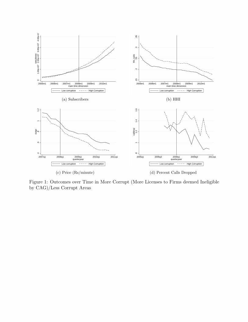
the difference-in-difference analysis. For example, a graph of the time trend in subscribers

shows a divergence between corrupt and less corrupt regions prior to the license allocation

34Tables A.2 and A.3 in the Appendix also show the basic difference-in-differences estimate without timeor region fixed effects.

35Note that the number of clusters in some of the regressions may be low: for example, there are 22 regions,16 quarters, and only 4 telecom circles in the dataset. As a robustness check, I run percentile-t wild clusterbootstraps as suggested by Cameron et al. (2008) in all cases. This does not change inferences drawn fromclustering on region or quarter dimensions. It does, however, make a large difference to inference based onclustering at the circle level, which is not surprising since there are only four circle clusters. Hence, for theseregressions – ones with price and minutes of use as outcomes – I present the p-values from the percentile-twild cluster bootstraps instead of standard errors.

14

process (Figures 1 and 2). This is also true for log subscribers, prices, and revenues –

with more corrupt areas growing faster or declining less slowly than less corrupt areas –

but not in general true for the quality variables. Moreover, general economic trends do

not seem to be different between corrupt and less corrupt areas, as shown in Figure 3.

Nonetheless, to account for this potential confound, I add region-specific time trends as

a control:

Yst = α+ β(Post ∗ Corrupt)st + γ(AmtSpectrum)st (4)

+∑t

Timet +∑s

Regions +∑s

Regions ∗ Timet + εst

Note that this estimation might conflate any dynamic effects of the license allocation

with the region-specific time trends (Wolfers, 2006). To separate out these effects, I

include indicators for time periods in the post period in corrupt areas, and run the

following estimation:

Yst = α+ γ(AmtSpectrum)st +∑k≥1

βkK periods after allocation in corrupt areasst (5)

+∑t

Timet +∑s

Regions +∑s

Regions ∗ Timet + εst

The coefficients βk are presented in Figure 4.

Despite the evidence presented in the previous section which suggested that defence

requirements drove the license allocation, it is possible that other unobserved factors were

involved. For example, the corrupt allocation may have been driven by unobserved future

potential for growth. To the extent that this potential was predicted by pre-existing trends

and fixed regional characteristics – and as the results below suggest, these do indeed have

very high predictive power – the inclusion of fixed effects and trends ameliorates some of

these concerns. To the extent that unobserved factors beyond these controls may have

influenced outcomes, the results below must be interpreted with caution.

4 Results

A glance at Table 4 suggests that the corrupt sale of licenses had no significant effects

on the number of wireless telephone subscribers (Panel A, columns 1 and 3). The results

are similar if the proportion of new licenses received illegally in each region is consid-

ered rather than a simple categorization into more versus less corrupt regions (Panel

B, columns 1 and 3). When region-specific linear time trends are introduced into the

regressions, the coefficient drops dramatically, and even turns negative (column 4), al-

15

though the magnitudes are tiny (less than 0.002 standard deviations). The dynamics of

the post-allocation period, shown in Figures 4a and 4b, suggest that these trends are not

conflating dynamic effects.36

While determining whether results are precisely estimated is a somewhat subjective

exercise, and the standard errors used are conservative (multi-way clustered at the region

and time levels), these results suggest that the difference between more and less corrupt

regions was a narrowly estimated zero (standard errors on the order of 200,000 or about

1.5% of the standard deviation, or 1.2% of the mean) at least for the first year after

the license allocations. After this period, while the standard errors increase, so does the

magnitude of the coefficients. Hence, even at the end of twenty four months after the new

licenses were allotted, the 95% confidence intervals allow us to rule out negative effects

greater than 0.01 standard deviations.

How did the corrupt allocation affect firm revenues? Revenues might be interpreted as

an indicator of profitability of firms in the region. This outcome is only available for GSM

providers, so the results must be interpreted with caution. Nonetheless, Table 4 presents

some evidence that firms in more corrupt regions seem to have significantly increased

revenue levels after the allocation, with increases of 25% seen in Panel A, columns 5-8.

This does not seem to be true when the outcome is specified in logs rather than levels

(Table A.8). The results also disappear when the dynamics of the post period are taken

into account (Figure 4).

The corrupt license allocation also does not seem to have negatively affected con-

sumers. Data on the quality of service provided, such as the proportion of calls dropped

or TRAI measures of average voice quality, suggest that more corrupt areas were again

similar to less corrupt areas after the license allocation. The results indicate that, if

anything, quality improved in more corrupt areas after the allocation.

Results on prices paid per minute and minutes used must be interpreted with two

caveats in mind: first, the data are aggregated at a higher level (to categories of regions

called “circles”) and hence coefficients are not directly comparable; and second since there

are only four region categories, clustered standard errors can be inappropriate. Table 6

hence shows p-values from a wild cluster percentile-t bootstrap (Cameron et al., 2008)

instead of standard errors. The results again suggest that neither prices per minute

nor minutes used per subscriber were consistently significantly different in more corrupt

circles post allocation.

36Given that the average number of subscribers in corrupt versus less corrupt areas was quite differentprior to the allocation of licenses, difference-in-differences estimations will be sensitive to the functional form.The log results mostly mirror the levels results: corrupt areas do not appear to be significantly different thanless corrupt areas post allocation (Table A.8).

16

4.1 Robustness checks

The results above are robust to a variety of checks. The first check changes the definition

of the post period to the period after spectrum, rather than licenses, is assigned. Spectrum

was allocated as soon as it was available; some spectrum may have been vacant at the

time of license allocation, while other pieces may have been in use by the defense forces.

The advantage of this definition is that it better captures when a firm can actually

start operating; moreover, the empirical specification corresponds better to a standard

state-level difference-in-differences based on differential timing of policy changes. The

disadvantage is that the timing may be endogenous, given that corrupt firms might have

been able to influence the spectrum allocation date. In any case, using either the date

when the first firm received new spectrum in a region or the date when all firms had

received their allotment does not qualitatively change the results described above, as

shown in tables A.4-A.7.

A second robustness check changes the empirical methodology used to the synthetic

control method developed by Abadie and Gardeazabal (2003) and Abadie et al. (2010).

This method for causal inference “provides a data-driven procedure to construct synthetic

control units based on a convex combination of comparison units that approximates the

characteristics of the unit that is exposed to the intervention.” The synthetic control

group is constructed using pre-intervention characteristics – in this case I use controls

including population, literacy, and state GDP, as well as cumulative spectrum availability

in various bands and pre-period outcomes. Since the method is designed for estimating

effects in settings where a single unit is exposed to treatment, and in this case there

are more units exposed to “treatment” rather than “control”, I flip the designation of

treatment in order to allow for a larger set of potential control units, and also collapse the

new treated units into one using simple averaging as suggested by the method’s creators.

Figures A.1 and A.3 show predicted outcomes for the synthetic control group (the

more corrupt areas in this case) versus the treatment group (the less corrupt areas).

As is clear from the figures, the outcomes basically line up exactly post allocation of

licenses. This is particularly true in cases where the pre-period outcomes can be precisely

predicted. Where pre-period outcomes cannot be precisely predicted, the post-allocation

outcomes of the groups are not as well aligned.37

37Inference in this method is through the use of placebo tests in which the synthetic control method isapplied to areas which actually did not receive the intervention. The gap between treatment and syntheticcontrol groups is compared to the gaps between the placebo treatment and synthetic control groups. AsFigures A.2 and A.4 show, the actual gap is in fact much smaller than the placebo gaps, suggesting thatthere is no effect of the corrupt allocation.

17

5 Discussion and conclusion

Overall, the estimations suggest that the corrupt allocation had, at worst, no measurable

impact on activity in wireless telecom markets, which runs counter to much of the macro-

and micro-economic evidence on the impact of corruption, as well as the perception (in

India at least) of the effect of corruption scandals on growth. For example, Mauro (1995)

suggests that improving a country’s corruption index score by one standard deviation

would lead to a 0.8 percentage point increase in the annual growth rate of GDP. In

the micro-economic literature, Fisman and Svensson (2007) find that a one percentage

point increase in bribes reduces annual firm growth by three percentage points; Djankov

and Sequeira (2010) find that firms suffer costs on average three to four times higher

than actual bribes paid for transport to ports with lower corruption; and Ferraz et al.

(2010) show educational outcomes to be 0.35 standard deviations lower in corrupt areas

as compared to areas without corruption.

What might explain this discord? First, despite the restrictions on direct sale and

transfer of licenses and spectrum, firms who illegitimately received the licenses trans-

ferred them to other firms through complex series of mergers and acquisitions. Table 7

tracks licenses from initial allocation to eventual user. It shows, for example, that the

shell company Swan was acquired by UAE telecom giant Etisalat. Licenses held by a

group of real estate companies (Allianz and Unitech) were eventually obtained by the

Norwegian firm Telenor. Eventually, 83 of the 122 licenses allocated (68%) were acquired

by other firms through mergers or dilution of equity. Such transfers have occurred in

other countries as well, when the initial licensee was not necessarily set up to efficiently

provide wireless telecom service: for example, McMillan (1994) recounts the case of an

“obscure group” obtaining via lottery a license to provide wireless service on Cape Cod

(in the US) and promptly selling it on to Southwestern Bell for a large profit. Since there

were more corruptly allocated licenses in more corrupt areas (by definition), there were

significantly more mergers in these areas (29% of all licensed entities) as opposed to the

less corrupt areas (23%).

However, the transfer of licenses to other firms does not seem sufficient, by itself,

to explain why corruption had no impact. Milgrom (2001) writes, for example, that

“the history of the US wireless telephone service offers direct evidence that the frag-

mented and inefficient initial distribution of rights was not quickly correctable by market

transactions”. There is no guarantee that the firms that obtained licenses through sec-

ondary transfers were necessarily efficient: for example, it is possible that efficient yet

law-abiding firms may not necessarily wish to obtain corruptly acquired assets. If ac-

quiring licenses and licenses confers monopoly power to the new firms, they may pass on

costs to customers: in India, anecdotal evidence suggests that monopoly power wielded by

coal-mining companies (who also procured licenses to coal mines in a corrupt allocation

process) was responsible for efficiency losses in that sector (Times of India, 2012).

18

In the case of the 2G allocation, the degree of competitiveness in the wireless telecom

market may have forced new entrants to provide services efficiently. As described above,

wireless telecom markets in India tend to be characterized by aggressive competition for

subscribers. There were 6.6 providers on average per region prior to the new alloca-

tion, but by December 2010, following new allocation and consolidation, there were 12.2

providers per region. Of course, some of these new providers could be small and incon-

sequential, but other more reliable measures also suggest large increases in competition.

In both corrupt and non-corrupt areas, the four largest firms only held about 55-59% of

market share.

Figure 2b suggests that competitiveness, as measured by the HHI of market share,

increased dramatically after the new spectrum allocation in both types of regions, after

a brief lag possibly related to the actual handover of spectrum and setting up of new

service providers. The HHI dropped from an average of 2,233 points in January 2008 to

an average of 1,710 by December 2010, a drop of 23.4 percent. For context, a merger

that would increase concentration by 200 points in already concentrated markets would

be presumed “likely to enhance market power” and hence come under scrutiny by the US

Department of Justice and the Federal Trade Commission. In comparison, a 513-point

drop appears to be a substantial increase in competition (U.S. Department of Justice and

the Federal Trade Commission, 2010). Meanwhile, the drops in corrupt and non-corrupt

regions appear to be relatively similar.

Regression analysis confirms this story. Table 8 shows that the effect of the new

allocation on HHI in corrupt regions was basically indistinguishable from that in less

corrupt regions. With the inclusion of region-specific trends, it appears as though there

was perhaps a small increase in competitiveness, although the effect sizes are small.

Moreover, Figure 4f suggests that some of this effect might be a conflation of the dynamics,

likely related to the lag in HHI decline after the allocation.

A final piece of evidence on competitiveness is provided by data on telecom firm profits

around the world (Telecom Regulatory Authority of India, 2012). A comparison of 31

global telecom companies shows that the three Indian companies in the sample are all in

the bottom half in terms of profits before taxes, with the best-performing Indian company

at number 20 in the rankings. Moreover, the three Indian companies are the top three in

the list of companies with the biggest decline in profits in the year 2010.

Thus, the Indian wireless telecom sector was more competitive than wireless telecom

sectors in other countries to begin with, and competition increased even further with

the allocation of new licenses. The fact that changes in market structure were similar

across corrupt and less corrupt regions might at least partly explain why changes in

other outcomes were also similar. Overall, in the Indian 2G spectrum case it appears

that the Coase theorem (Coase, 1959, 1960) applies – the initial misallocation of licenses

19

was corrected through the secondary market.38

In summary, then, this paper has investigated the impact of the corrupt allocation

of wireless licenses and spectrum on activity in the cellular telecom market in India. I

find that although many firms received licenses who had no prior experience in providing

wireless services, this had, at worst, no measurable impact on the number of wireless

subscribers, revenues, prices, usage, or measures of quality. The lack of an effect of cor-

ruption on consumer markets may be explained by a combination of factors: one potential

explanation is that the licenses were transferred to other firms better equipped to provide

wireless telecom services, and another may be the presence of existing large players and

competition in the wireless telecom market. The same corruption was, however, very

costly to the Indian government in terms of lost revenues. Moreover, the ensuing scandal

carries with it potential – but not easily measurable – social and political costs associated

with decreasing levels of public trust and rising cronyism. Nonetheless, under the con-

ditions of competitive markets and secondary license transfers, the corrupt allocation of

licenses to ill-equipped firms did not result in efficiency costs passed on to the consumer,

and the initial allocation of property rights did not matter.

38It is of course possible that despite the apparent efficient reallocation there were large transactions costsin the transfer. One such cost is delay in starting service. However, these delays were no different for licensesthat were reallocated as compared to those that were not, and also no different for the corruptly allocatedversus non-corruptly allocated licenses.

20

References

Abadie, Alberto, Alexis Diamond, and Jens Hainmueller, “Synthetic ControlMethods for Comparative Case Studies: Estimating the Effect of Californias TobaccoControl Program,,” Journal of the American Statistical Association, 2010, 105 (490),493–505.

and Javier Gardeazabal, “The Economic Costs of Conflict: A Case Study of theBasque Country,” American Economic Review, 2003, 93 (1), 113–132.

Aridjis, Homero, “The Sun, the Moon, and Walmart,” New York Times, April 30 2012.

Bertrand, Marianne, Simeon Djankov, Rema Hanna, and Sendhil Mul-lainathan, “Obtaining a Driver’s License in India: An Experimental Approach toStudying Corruption,” The Quarterly Journal of Economics, November 2007, 122 (4),1639–1676.

Cameron, Colin, Jonah Gelbach, and Doug Miller, “Bootstrap-Based Improve-ments for Inference with Clustered Errors,” Review of Economics and Statistics, 2008,90 (3), 414–427.

, , and , “Robust Inference with Multi-Way Clustering,” Journal of Business andEconomic Statistics, 2011, 29 (2), 238–249.

Coase, Ronald, “The Federal Communications Commission,” Journal of Law and Eco-nomics, 1959, 2, 1–40.

, “The Problem of Social Cost,” Journal of Law and Economics, 1960, 3, 1–44.

Comptroller & Auditor General of India, “Issue of Licenses and Allocation of 2GSpectrum,” Performance Audit Report 19, Union Government of India 2010.

Cramton, Peter, Evan Kwerel, Gregory Rosston, and Andrzej Skrzypacz,“Using Spectrum Auctions to Enhance Competition in Wireless Services,” Journal ofLaw and Economics, 2011, 54 (4), S167–88.

Djankov, Simeon and Sandra Sequeira, “An Empirical Study of Corruption inPorts,” mimeo, LSE 2010.

Ferraz, Claudio, Frederico Finan, and Diana Moreira, “Corrupting Learning:Evidence from Missing Federal Education Funds in Brazil,” Technical Report, UCBerkeley April 2010.

Fisman, Raymond and Jakob Svensson, “Are Corruption and Taxation ReallyHarmful to Growth? Firm Level Evidence,” Journal of Development Economics, May2007, 83 (1), 63–75.

Griliches, Zvi, “Hybrid Corn: An Exploration in the Economics of TechnologicalChange,” Econometrica, October 1957, 25, 501–22.

Hazlett, Thomas, “The Rationality of U. S. Regulation of the Broadcast Spectrum,”Journal of Law and Economics, 1990, 33 (1), 133–75.

21

, “Property Rights and Wireless License Values,” Journal of Law and Economics, 2008,51 (3), 563–98.

and Roberto Munoz, “A Welfare Analysis of Spectrum Allocation Policies,” TheRAND Journal of Economics, 2009, 40 (3), 424–54.

Hunt, Jennifer, “How Corruption Hits People When they are Down,” Journal of De-velopment Economics, November 2007, 84 (2), 574–589.

Huntington, Samuel, “Modernisation and Corruption,” in “Political Order in ChangingSocieties,” New Haven: Yale University Press, 1968.

Klemperer, Paul, “What Really Matters in Auction Design,” Journal of EconomicPerspectives, 2002, 16.

Kotwal, Ashok, Bharat Ramaswami, and Wilima Wadhwa, “Economic Liberal-ization and Indian Economic Growth: What’s the Evidence?,” Journal of EconomicLiterature, 2011, 49 (4), 1152–99.

Leff, Nathaniel, “Economic Development through Bureaucratic Corruption,” AmericanBehavioural Scientist, 1964, 8, 8–14.

Lui, Francis, “An Equilibrium Queuing Model of Bribery,” Journal of Political Econ-omy, 1985, 93 (4), 760–81.

Mauro, Paolo, “Corruption and Growth,” The Quarterly Journal of Economics, August1995, 110 (3), 681–712.

McMillan, John, “Selling Spectrum Rights,” Journal of Economic Perspectives, 1994,8.

Melody, William, “Radio Spectrum Allocation: Role of the Market,” American Eco-nomic Review Papers and Proceedings, 1980, 70 (2), 393–97.

Milgrom, Paul, Putting Auction Theory to Work, New York: Cambridge UniversityPress, 2001.

Murphy, Kevin M, Andrei Shleifer, and Robert W Vishny, “Why Is Rent-SeekingSo Costly to Growth?,” American Economic Review, May 1993, 83 (2), 409–14.

Niehaus, Paul and Sandip Sukhtankar, “Corruption Dynamics: the Golden GooseEffect,” American Economic Journal: Economic Policy, November 2013, 5 (4), 230–69.

and , “The Marginal Rate of Corruption in Public Programs: Evidence from India,”Journal of Public Economics, July 2013, 104, 52 – 64.

Olken, Benjamin A., “Corruption and the Costs of Redistribution: Micro Evidencefrom Indonesia,” Journal of Public Economics, May 2006, 90 (4-5), 853–870.

, “Monitoring Corruption: Evidence from a Field Experiment in Indonesia,” Journalof Political Economy, April 2007, 115 (2), 200–249.

and Patrick Barron, “The Simple Economics of Extortion: Evidence from Truckingin Aceh,” Journal of Political Economy, 06 2009, 117 (3), 417–452.

22

and Rohini Pande, “Corruption in Developing Countries,” Annual Review of Eco-nomics, 2012, 4 (1).

Patil, Justice Shivaraj V., “Examination of Appropriateness of Procedures Followedby Department of Telecommunications in Issuance of Licenses and Allocation of Spec-trum During the Period 2001-2009,” Report, Supreme Court of India 2011.

Reinikka, Ritva and Jakob Svensson, “Local Capture: Evidence From a CentralGovernment Transfer Program in Uganda,” The Quarterly Journal of Economics, May2004, 119 (2), 678–704.

Shleifer, Andrei and Daniel Treisman, “A Normal Country: Russia After Commu-nism,” Journal of Economic Perspectives, 2005, 19 (1), 151–174.

and Robert W Vishny, “Corruption,” The Quarterly Journal of Economics, August1993, 108 (3), 599–617.

Singhvi, G.S. and Asok Kumar Ganguly, “Judgment on Writ Petitions No 423 of2010 and 10 of 2011,” Judgment, Supreme Court of India 2012.

Skinner, Jonathan and Douglas Staiger, “Technology Adoption from Hybrid Cornto Beta-Blockers,” in “Hard-to-Measure Goods and Services: Essays in Honor of ZviGriliches,” University of Chicago Press and NBER, 2007.

Svensson, Jakob, “Who Must Pay Bribes And How Much? Evidence From A CrossSection Of Firms,” The Quarterly Journal of Economics, February 2003, 118 (1), 207–230.

Telecom Regulatory Authority of India, “Telecommunications in Select CountriesPolicies - Statistics,” Report, Telecom Regulatory Authority of India 2012.

Thompson, Samuel B., “Simple formulas for standard errors that cluster by both firmand time,” Journal of Financial Economics, January 2011, 99 (1), 1–10.

Times of India, “After CBI Raids, Companies Linked to Raja Put up a Brave Front,”December 18 2010.

, “Secret of Jindals Success: Cheap Coal, Costly Power,” September 9 2012.

U.S. Department of Justice and the Federal Trade Commission, “HorizontalMerger Guidelines,” Report, USDOJ 2010.

Wolfers, Justin, “Did Unilateral Divorce Laws Raise Divorce Rates? A Reconciliationand New Results,” American Economic Review, December 2006, 96 (5), 1802–20.

Xu, Beina, “Governance in India: Corruption,” Background Report, Council on ForeignRelations 2013.

23

01.

00e+

072.

00e+

073.

00e+

074.

00e+

07to

tsub

new

2005m1 2006m1 2007m1 2008m1 2009m1 2010m1main time dimension

Low corruption High Corruption

(a) Subscribers

.15

.2.2

5.3

.35

hhi_

subs

2005m1 2006m1 2007m1 2008m1 2009m1 2010m1main time dimension

Low corruption High Corruption

(b) HHI

.4.6

.81

1.2

outg

o

2007q1 2008q1 2009q1 2010q1 2011q1quarteryear

Low corruption High Corruption

(c) Price (Rs/minute)

.81

1.2

1.4

1.6

calld

rop

2005q1 2006q3 2008q1 2009q3 2011q1quarteryear

Low corruption High Corruption

(d) Percent Calls Dropped

Figure 1: Outcomes over Time in More Corrupt (More Licenses to Firms deemed Ineligibleby CAG)/Less Corrupt Areas

01.

00e+

072.

00e+

073.

00e+

074.

00e+

07to

tsub

new

2005m1 2006m1 2007m1 2008m1 2009m1 2010m1main time dimension

Low corruption High Corruption

(a) Subscribers

.15

.2.2

5.3

.35

hhi_

subs

2005m1 2006m1 2007m1 2008m1 2009m1 2010m1main time dimension

Low corruption High Corruption

(b) HHI

.4.6

.81

1.2

outg

o

2007q1 2008q1 2009q1 2010q1 2011q1quarteryear

Low corruption High Corruption

(c) Price (Rs/minute)

11.

21.

41.

6ca

lldro

p

2005q1 2006q3 2008q1 2009q3 2011q1quarteryear

Low corruption High Corruption

(d) Percent Calls Dropped

Figure 2: Outcomes over Time in More Corrupt (More Licenses to CBI Indicted Firms)/LessCorrupt Areas

2000

030

000

4000

050

000

6000

0sd

p_ca

p

2000 2005 2010year

Low corruption High Corruption

(a) GDP/capita

9.5

1010

.511

lnsd

p_ca

p2000 2005 2010

year

Low corruption High Corruption

(b) Log GDP/capita

2000

030

000

4000

050

000

sdp_

cap

2000 2005 2010year

Low corruption High Corruption

(c) GDP/capita

9.8

1010

.210

.410

.610

.8ln

sdp_

cap

2000 2005 2010year

Low corruption High Corruption

(d) Log GDP/capita

Figure 3: GDP/capita Trends

In panels (a) and (b), high corruption refers to areas where relatively more licenses were declared ineligible

by the CAG. In panels (c) and (d), high corruption refers to areas where relatively more firms were indicted

by the CBI.

−50

0000

00

5000

000

1000

0000

tots

ubne

w

0 10 20 30 40monthafter

(a) Subscribers

−50

0000

00

5000

000

1000

0000

1500

0000

tots

ubne

w

0 10 20 30 40monthafter

(b) Subscribers

−15

0−

100

−50

050

100

reve

nue_

op

0 5 10qafter

Low Corruption Mid−Low CorruptionMid Corruption Mid−High CorruptionHigh Corruption Highest Corruption

(c) Operator Revenues (Rs 10 Million)

−10

0−

500

5010

0re

venu

e_op

0 5 10qafter

Low Corruption Mid−Low CorruptionMid−High Corruption High CorruptionHighest Corruption

(d) Operator Revenues (Rs 10 Million)

−.1

−.0

50

.05

hhi_

subs

0 10 20 30 40monthafter

(e) HHI

−.0

8−

.06

−.0

4−

.02

0.0

2hh

i_su

bs

0 10 20 30 40monthafter

(f) HHI

Figure 4: Dynamics of Post Period in More Corrupt Areas

Plots coefficients on indicators for month/quarter post license allocation in corrupt areas. Panels (a), (b), (e)

and (f) also plot standard errors. In panels (a), (c), and (e), more corrupt areas are those where relatively

more licenses were declared ineligible by the CAG, while in panels (b), (d), and (f), they are areas where

relatively more firms were indicted by the CBI. The lowest corruption region is the comparison region in

panels (c)-(d).

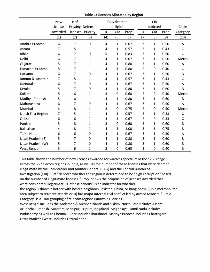
Table 1: Licenses Allocated by Region

New # of CAG deemed CBI

Licenses Existing Defense Ineligible Indicted Circle

Awarded Licenses Priority # Cat Prop # Cat Prop Category

(1) (2) (3) (4) (5) (6) (7) (8) (9) (10)

Andhra Pradesh 6 7 0 4 1 0.67 3 1 0.50 A

Assam 7 5 1 4 1 0.57 3 1 0.43 C

Bihar 6 7 0 5 1 0.83 3 1 0.50 C

Delhi 6 7 1 4 1 0.67 3 1 0.50 Metro

Gujarat 5 7 1 4 1 0.80 3 1 0.60 A

Himachal Pradesh 5 7 1 4 1 0.80 2 0 0.40 C

Haryana 6 7 0 4 1 0.67 3 1 0.50 B

Jammu & Kashmir 7 5 1 4 1 0.57 3 1 0.43 C

Karnataka 6 7 0 4 1 0.67 3 1 0.50 A

Kerala 5 7 0 4 1 0.80 3 1 0.60 B

Kolkata 5 6 1 3 0 0.60 2 0 0.40 Metro

Madhya Pradesh 5 6 1 4 1 0.80 3 1 0.60 B

Maharashtra 6 7 0 4 1 0.67 3 1 0.50 A

Mumbai 4 8 1 3 0 0.75 2 0 0.50 Metro

North East Region 7 5 1 4 1 0.57 3 1 0.43 C

Orissa 6 6 1 4 1 0.67 2 0 0.33 C

Punjab 5 8 1 3 0 0.60 3 1 0.60 B

Rajasthan 4 8 1 4 1 1.00 3 1 0.75 B

Tamil Nadu 6 6 0 4 1 0.67 3 1 0.50 A

Uttar Pradesh (E) 5 7 0 4 1 0.80 3 1 0.60 B

Uttar Pradesh (W) 5 7 0 4 1 0.80 3 1 0.60 B

West Bengal 5 6 1 3 0 0.60 2 0 0.40 B

This table shows the number of new licenses awarded for wireless spectrum in the "2G" range 

across the 22 telecom regions in India, as well as the number of these licenses that were deemed 

illegitimate by the Comptroller and Auditor General (CAG) and the Central Bureau of 

Investigation (CBI). "Cat" denotes whether the region is determined to be "high corruption" based

on the number of illegitimate licenses. "Prop" shows the proportion of licenses awarded that 

were considered illegitimate. "Defense priority" is an indicator for whether

the region i) shares a border with hostile neighbors Pakistan, China, or Bangladesh ii) is a metropolitan 

area subject to terrorist attacks or iii) has major internal civil conflict led by armed Maoists. "Circle

Category" is a TRAI grouping of telecom regions (known as "circles").

West Bengal includes the Andaman & Nicobar Islands and Sikkim. North East includes Assam

Arunachal Pradesh, Mizoram, Manipur, Tripura, Nagaland, Meghalaya. Tamil Nadu includes

Puducherry as well as Chennai. Bihar includes Jharkhand. Madhya Pradesh includes Chattisgarh.

Uttar Pradesh (West) includes Uttarakhand

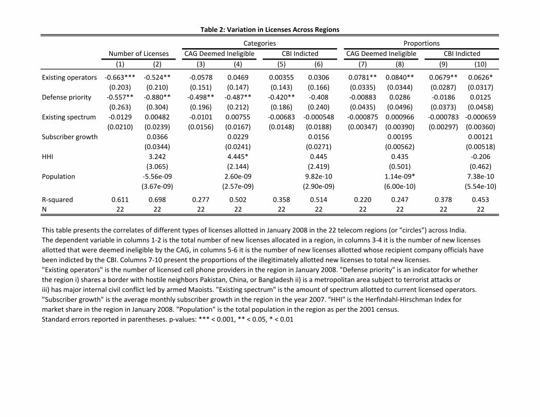
Table 2: Variation in Licenses Across Regions

Categories Proportions

Number of Licenses CAG Deemed Ineligible CBI Indicted CAG Deemed Ineligible CBI Indicted

(1) (2) (3) (4) (5) (6) (7) (8) (9) (10)

Existing operators ‐0.663*** ‐0.524** ‐0.0578 0.0469 0.00355 0.0306 0.0781** 0.0840** 0.0679** 0.0626*

(0.203) (0.210) (0.151) (0.147) (0.143) (0.166) (0.0335) (0.0344) (0.0287) (0.0317)

Defense priority ‐0.557** ‐0.880** ‐0.498** ‐0.487** ‐0.420** ‐0.408 ‐0.00883 0.0286 ‐0.0186 0.0125

(0.263) (0.304) (0.196) (0.212) (0.186) (0.240) (0.0435) (0.0496) (0.0373) (0.0458)

Existing spectrum ‐0.0129 0.00482 ‐0.0101 0.00755 ‐0.00683 ‐0.000548 ‐0.000875 0.000966 ‐0.000783 ‐0.000659

(0.0210) (0.0239) (0.0156) (0.0167) (0.0148) (0.0188) (0.00347) (0.00390) (0.00297) (0.00360)

Subscriber growth 0.0366 0.0229 0.0156 0.00195 0.00121

(0.0344) (0.0241) (0.0271) (0.00562) (0.00518)

HHI 3.242 4.445* 0.445 0.435 ‐0.206

(3.065) (2.144) (2.419) (0.501) (0.462)

Population ‐5.56e‐09 2.60e‐09 9.82e‐10 1.14e‐09* 7.38e‐10

(3.67e‐09) (2.57e‐09) (2.90e‐09) (6.00e‐10) (5.54e‐10)

R‐squared 0.611 0.698 0.277 0.502 0.358 0.514 0.220 0.247 0.378 0.453

N 22 22 22 22 22 22 22 22 22 22

This table presents the correlates of different types of licenses allotted in January 2008 in the 22 telecom regions (or "circles") across India.

The dependent variable in columns 1‐2 is the total number of new licenses allocated in a region, in columns 3‐4 it is the number of new licenses

allotted that were deemed ineligible by the CAG, in columns 5‐6 it is the number of new licenses allotted whose recipient company officials have

been indicted by the CBI. Columns 7‐10 present the proportions of the illegitimately allotted new licenses to total new licenses.

"Existing operators" is the number of licensed cell phone providers in the region in January 2008. "Defense priority" is an indicator for whether

the region i) shares a border with hostile neighbors Pakistan, China, or Bangladesh ii) is a metropolitan area subject to terrorist attacks or 

iii) has major internal civil conflict led by armed Maoists. "Existing spectrum" is the amount of spectrum allotted to current licensed operators.

"Subscriber growth" is the average monthly subscriber growth in the region in the year 2007. "HHI" is the Herfindahl‐Hirschman Index for 

market share in the region in January 2008. "Population" is the total population in the region as per the 2001 census.

Standard errors reported in parentheses. p‐values: *** < 0.001, ** < 0.05, * < 0.01

Table 3: Summary Statistics and Balance

Test of equality

Average More corrupt Less corrupt (p‐value) Units

(1) (2) (3) (4) (5)

Subscribers 13,200,000  13,500,000  11,600,000  0.97

(12,600,000) (13,400,000) (7,978,902)

Ln(subscribers) 15.86 15.82775 15.98328 0.40

(1.19) (1.25) (0.84)

HHI 0.23 0.23 0.2 0.08

(0.08) (0.08) (0.03)

Revenues 132.03 132.63 129.31 0.55 Rs 10 million

(94.6) (99.66) (67.61)

Ln(revenues) 4.54 4.51 4.69 0.41

(0.93) (0.98) (0.67)

% calls dropped 1.32 1.37 1.12 0.60

(0.55) (0.59) (0.31)

Voice quality 97.35 97.26 97.78 0.24 Index 1‐100

(1.2) (1.28) (0.59)

Minutes used 431.05 419.69 442.40 0.17 Per month

(51.13) (51.35) (49.09)

Price/minute 0.77 0.82 0.71 0.55 Rupees

(0.21) (0.19) (0.22)

"More" and "less" corrupt refer to regions categorized in column 5 of Table 1. "p‐value"

is the p‐value of the difference in outcomes in regions prior to January 2008.

"Subscribers" is the total number of wireless subscribers in a telecom region (monthly, 2005‐10).

"HHI" is the Herfindahl‐Hirschman index of market concentration (monthly, 2005‐10).

"Revenues" are averages per operator across GSM operators in the region (quarterly, 2005‐10).

All other variables are subscriber‐weighted averages across all operators in the region.

"% calls dropped" is the percentage of calls that were cut off before speaking subscribers had

terminated the call, while "voice quality" is the clarity of the sound transfer in a call measured on

an index from 1‐100 (both quarterly, 2007‐10).  "Minutes used" are the total number of minutes

Table 4: Subscribers and Revenues

Subscribers Revenues

CAG Deemed Ineligible CBI Indicted CAG Deemed Ineligible CBI Indicted

(1) (2) (3) (4) (5) (6) (7) (8)

PANEL A: Simple dif‐in‐dif

Corrupt x post 647,357 71,220 416,778 ‐22,149 17.99 25.01* 23.86 28.61**

(414,917) (304,027) (457,242) (338,081) (13.71) (13.67) (15.17) (13.87)

Adj R‐squared 0.988 0.999 0.988 0.999 0.958 0.974 0.958 0.975

PANEL B: Dif‐in‐dif with proportion new licenses

Corrupt x post 123,268 ‐1.469e+06 1.004e+06 ‐541,195 31.19 39.82 77.46* 89.04*

(2.993e+06) (2.355e+06) (2.915e+06) (2.220e+06) (41.98) (43.56) (43.39) (45.83)

Adj R‐squared 0.988 0.999 0.988 0.999 0.957 0.974 0.958 0.974

Region FE Yes Yes Yes Yes Yes Yes Yes Yes

Time FE Yes Yes Yes Yes Yes Yes Yes Yes

Region x Time No Yes No Yes No Yes No Yes

N 1584 1584 1584 1584 1584 1584 1584 1584

The dependent variable in columns 1‐4 is the total number of wireless telecom subscribers in a region‐month. In columns

5‐8 it is the log of subscribers. In Panel A, "Corrupt" is an indicator for whether the region has a high number of 

illegitimately allotted licenses as determined by the CAG or CBI. In Panel B, "Corrupt" is the proportion of illegitimately

allotted licenses to all new licenses. In both panels, "Post" is an indicator for months after February 2008.

Standard errors in parentheses are multi‐way clustered by month as well as region. p‐values: *** < 0.001, ** < 0.05, * < 0.01

Table 5: Measures of Quality

Percent Calls Dropped Voice Quality

CAG Deemed Ineligible CBI Indicted CAG Deemed Ineligible CBI Indicted

(1) (2) (3) (4) (5) (6) (7) (8)

PANEL A: Simple dif‐in‐dif

Corrupt x post 0.263** 0.148 0.194 0.0772 ‐0.431 ‐0.171 ‐0.275 ‐0.00657

(0.106) (0.149) (0.135) (0.147) (0.381) (0.398) (0.368) (0.374)

Adj R‐squared 0.117 0.488 0.100 0.487 0.087 0.568 0.117 0.588

PANEL B: Dif‐in‐dif with proportion new licenses

Corrupt x post ‐1.655** ‐1.842** ‐1.665** ‐1.994* 3.304* 3.652* 3.336** 3.989**

(0.743) (0.926) (0.831) (1.056) (1.961) (2.022) (1.685) (2.021)

Adj R‐squared 0.112 0.511 0.102 0.508 0.097 0.568 0.083 0.586

Region FE Yes Yes Yes Yes Yes Yes Yes Yes

Time FE Yes Yes Yes Yes Yes Yes Yes Yes

Region x Time No Yes No Yes No Yes No Yes

N 352 352 352 352 352 352 352 352

The dependent variable in columns 1‐4 is the average percent of dropped calls in a region‐quarter, while that in columns

5‐8 is the average voice quality (1‐100) in a region‐quarter. In Panel A, "Corrupt" is an indicator for whether the region 

has a high number of illegitimately allotted licenses as determined by the CAG or CBI. In Panel B, "Corrupt" is the proportion 

of illegitimately allotted licenses to all new licenses. In both panels, "Post" is an indicator for quarters after Q1 2008.

Standard errors in parentheses are multi‐way clustered by quarter as well as region. p‐values: *** < 0.001, ** < 0.05, * < 0.01

Table 6: Prices and Minutes Used

Price per minute Minutes used

CAG Deemed Ineligible CBI Indicted CAG Deemed Ineligible CBI Indicted

(1) (2) (3) (4) (5) (6) (7) (8)

PANEL A: Simple dif‐in‐dif

Corrupt x post ‐0.0221 0.0695 ‐0.0221 0.0695 52.34 53.36 52.34 53.36

{0.873} {0.583} {0.873} {0.293} {0.063} {0.193} {0.063} {0.193}

Adj R‐squared 0.898 0.963 0.898 0.963 0.820 0.848 0.820 0.848

PANEL B: Dif‐in‐dif with proportion new licenses

Corrupt x post 2.877 1.360* 1.816* 0.711 ‐474.8 ‐47.88 ‐408.5* ‐218.7

{0.213} {0.063} {0.063} {0.173} {0.448} {0.908} {0.068} {0.653}

Adj R‐squared 0.932 0.965 0.937 0.963 0.801 0.824 0.820 0.829

Region FE Yes Yes Yes Yes Yes Yes Yes Yes

Time FE Yes Yes Yes Yes Yes Yes Yes Yes

Region x Time No Yes No Yes No Yes No Yes

N 64 64 64 64 64 64 64 64

The dependent variable in columns 1‐4 is the average price per minute in a circle‐quarter, while that in columns 5‐8 is 

the average number of minutes per subscriber per month in a region‐quarter. In Panel A, "Corrupt" is an indicator for 

whether the region has a high number of illegitimately allotted licenses as determined by the CAG or CBI. In Panel B, 

"Corrupt" is the proportion of illegitimately allotted licenses to all new licenses. "Post" is an indicator for quarters after 

Q1 2008.

P‐values from a wild cluster percentile‐t bootstrap are reported in parentheses: *** < 0.001, ** < 0.05, * < 0.01

Table 7: Tracing Licenses

Eventual # New CAG deemed CBI

Original Company Operator Licenses Ineligible Indicted

(1) (2) (3) (4) (5)

Adonis Projects Pvt. Ltd. Uninor 6 1 1

Allianz Infratech Pvt. Ltd. Etisalat 2 1 1

Aska Projects Ltd. Uninor 3 1 1

Azare Properties Ltd. Uninor 1 1 1

Datacom Solutions Pvt. Ltd. Videocon 21 1 0

Hudson Properties Ltd. Uninor 1 1 1

Idea Cellular Ltd. Idea 9 0 0

Loop Telecom Private Ltd. Loop 21 1 1

Nahan Properties Pvt. Ltd. Uninor 6 1 1

S Tel Ltd. S Tel 6 1 0

Shyam Telelink Limited Sistema Shyam 21 0 0

Spice Communications Ltd. Idea 4 0 0

Swan Telecom Pvt. Ltd. Etisalat 13 1 1

Tata Teleservices Ltd. Tata Docomo 3 0 1

Unitech Builders & Estates Pvt. Ltd. Uninor 1 1 1

Unitech Infrastructures Pvt. Ltd. Uninor 1 1 1

Volga Properties Pvt. Ltd. Uninor 3 1 1

This table lists the original recipients of all 122 licenses granted in 2008, as well as the

eventual operators of wireless telecom service using these licenses. The shaded rows 

represent instances where the original and eventual company is the same entity. Note that

Tata Teleservices and S Tel both sold equity to other entities but retained over 50%.

Table 8: HHI

CAG Deemed Ineligible CBI Indicted

(1) (2) (3) (4)

PANEL A: Simple dif‐in‐dif

Corrupt x post ‐0.0108 0.00478 ‐0.0199** ‐0.00812

(0.00989) (0.0100) (0.00808) (0.0107)

Adj R‐squared 0.926 0.974 0.927 0.974

PANEL B: Dif‐in‐dif with proportion new licenses

Corrupt x post ‐0.0921 ‐0.0389 ‐0.134* ‐0.0760***

(0.0642) (0.0272) (0.0698) (0.0282)

Adj R‐squared 0.928 0.974 0.929 0.975

Region FE Yes Yes Yes Yes

Time FE Yes Yes Yes Yes

Region x Time No Yes No Yes

N 1584 1584 1584 1584

The dependent variable in all columns is the Herfindahl‐Hirshman index for 

market share of wireless subscribers in a region‐month. In Panel A, 

"Corrupt" is an indicator for whether the region has a high number of 

illegitimately allotted licenses as determined by the CAG or CBI. In Panel B, 

"Corrupt" is the proportion of illegitimately allotted licenses to all new 

licenses. In both panels, "Post" is an indicator for months after February 2008.

Standard errors in parentheses are multi‐way clustered by month as well as 

region. p‐values: *** < 0.001, ** < 0.05, * < 0.01

010

0000

0020

0000

0030

0000

00to

tsub

new

540 560 580 600 620monthyear

treated unit synthetic control unit

(a) Subscribers

.15

.2.2

5hh

i_su

bs540 560 580 600 620

monthyear

treated unit synthetic control unit

(b) HHI

5010

015

020

0re

venu

e_op

180 185 190 195 200 205quarteryear

treated unit synthetic control unit

(c) Operator Revenues (Rs 10 Million)

.91

1.1

1.2

1.3

1.4

calld

rop

185 190 195 200 205quarteryear

treated unit synthetic control unit

(d) Percent Calls Dropped

Figure A.1: Comparing Treatment and Synthetic Control Group Outcomes (where controlgroup is areas where more firms were deemed ineligible by CAG)

−2.

00e+

07−

1.00

e+07

01.

00e+

072.

00e+

07to

tsub

new

540 560 580 600 620monthyear

(a) Subscribers

−.0

50

.05

.1.1

5hh

i_su

bs

540 560 580 600 620monthyear

(b) HHI

−50

050

100

150

reve

nue_

op

180 185 190 195 200 205quarteryear

(c) Operator Revenues (Rs 10 Million)

−2

02

46

calld

rop

185 190 195 200 205quarteryear

(d) Percent Calls Dropped

Figure A.2: Synthetic Control Method Inference (CAG): Comparing Treatment-ControlGaps to Placebo Gaps

050

0000

0100

0000

0150

0000

0200

0000

0250

0000

0to

tsub

new

540 560 580 600 620monthyear

treated unit synthetic control unit

(a) Subscribers

.15

.2.2

5.3

.35

hhi_

subs

540 560 580 600 620monthyear

treated unit synthetic control unit

(b) HHI

4060

8010

012

014

0re

venu

e_op

180 185 190 195 200 205quarteryear

treated unit synthetic control unit

(c) Revenues (Rs 10 Million)

.91

1.1

1.2

1.3

1.4

calld

rop

185 190 195 200 205quarteryear

treated unit synthetic control unit

(d) Percent Calls Dropped

Figure A.3: Comparing Treatment and Synthetic Control Group Outcomes (where controlgroup is areas where more firms were indicted by CBI)

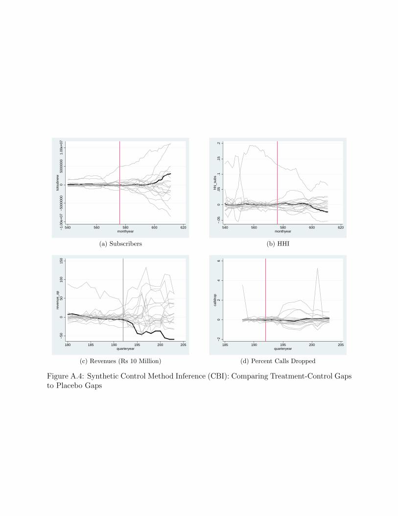
−1.

00e+

07−

5000

000

050

0000

01.

00e+

07to

tsub

new

540 560 580 600 620monthyear

(a) Subscribers

−.0

50

.05

.1.1

5.2

hhi_

subs

540 560 580 600 620monthyear

(b) HHI

−50

050

100

150

reve

nue_

op

180 185 190 195 200 205quarteryear

(c) Revenues (Rs 10 Million)

−2

02

46

calld

rop

185 190 195 200 205quarteryear

(d) Percent Calls Dropped

Figure A.4: Synthetic Control Method Inference (CBI): Comparing Treatment-Control Gapsto Placebo Gaps

Table A.1: Spectrum Allocation was Not Faster in Corrupt Areas

CAG CBI

(1) (2)

Time 0.572*** 0.461***

(0.134) (0.0954)

Corrupt 2.119 0.164

(1.406) (0.948)

Corrupt x Time ‐0.0809 0.0275

(0.145) (0.110)

N 352 352

This table presents maximum likelihood estimates of the 

proportion of spectrum actually distributed to allotted. Each

observation is a region‐month from Feb 2008‐May 2009, the

dates of the first and last distributions of new spectrum.

"Time" is a linear time trend. "Corrupt" is an indicator for

whether the region has a high number of illegitimately

allotted licenses as determined by the CAG or CBI.

Standard errors reported in parentheses. 

p‐values: *** < 0.001, ** < 0.05, * < 0.01

Table A.2: Basic Difference‐in Differences Specification for Outcomes in Tables 5, 6, and 10

Subscribers Percent calls dropped Voice quality Revenues HHI

CAG CBI CAG CBI CAG CBI CAG CBI CAG CBI

(1) (2) (3) (4) (5) (6) (7) (8) (9) (10)

PANEL A: Simple dif‐in‐dif

Corrupt 516,739 2.478e+06** 0.0369 0.000772 ‐0.181 ‐0.355 ‐63.06 76.65 0.0403* ‐0.0116

(1.028e+06) (1.122e+06) (0.169) (0.172) (0.269) (0.265) (96.54) (95.48) (0.0208) (0.0325)

Post ‐2.286e+06 ‐3.840e+06 0.0935 0.174 ‐0.584* ‐0.775** ‐234.0** ‐249.1** 0.0307 0.00556

(3.017e+06) (3.301e+06) (0.0982) (0.113) (0.355) (0.370) (96.78) (98.08) (0.0200) (0.0239)

Corrupt x post 3.237e+06 5.921e+06** 0.263** 0.194 ‐0.431 ‐0.275 135.9** 179.4*** ‐0.0125 0.0211

(2.570e+06) (2.720e+06) (0.106) (0.135) (0.381) (0.368) (60.04) (50.48) (0.0150) (0.0217)

Adj R‐squared 0.522 0.557 0.117 0.100 0.087 0.097 0.436 0.498 0.208 0.179

PANEL B: Dif‐in‐dif with proportion new licenses

Corrupt 3.635e+06 1.242e+07** 1.715** 1.576 ‐0.0897 ‐0.947 74.77 560.0* ‐0.187 ‐0.370***

(4.169e+06) (4.943e+06) (0.869) (1.137) (0.747) (0.953) (253.4) (309.7) (0.154) (0.140)

Post ‐1.637e+07** ‐1.625e+07*** 1.502** 1.163** ‐3.096* ‐2.512** ‐406.6*** ‐446.0*** ‐0.0822 ‐0.125***

(7.190e+06) (5.938e+06) (0.587) (0.486) (1.626) (1.140) (113.6) (103.5) (0.0652) (0.0426)

Corrupt x post 2.492e+07** 3.559e+07*** ‐1.655** ‐1.665** 3.304* 3.336** 423.2** 724.8*** 0.142 0.278***

(1.019e+07) (1.066e+07) (0.743) (0.831) (1.961) (1.685) (175.4) (168.5) (0.103) (0.0979)

Adj R‐squared 0.545 0.581 0.112 0.102 0.117 0.083 0.071 0.082 0.215 0.293

N 1584 1584 352 352 352 352 528 528 1584 1584

Presents the basic diffference‐in‐differences specification, with no region or time fixed effects, for the main paper outcomes. The only other

control variable included is the total amount of spectrum allocated in the region. 

Standard errors in parentheses are multi‐way clustered by time as well as region. p‐values: *** < 0.001, ** < 0.05, * < 0.01

Table A.3: Basic Dif‐in‐Difs Specification for Price and Minutes Used

Price Minutes

CAG CBI CAG CBI

(1) (2) (3) (4)

PANEL A: Simple dif‐in‐dif

Corrupt ‐0.03 ‐0.03 9.95 9.95

{0.61} {0.61} {0.59} {0.59}

Post ‐0.28 ‐0.28 ‐27.77 ‐27.77

{0.52} {0.52} {0.01} {0.01}

Corrupt x post 0.03 0.03 73.57 73.57

{0.74} {0.74} {0.11} {0.11}

Adj R‐squared 0.462 0.462 0.74 0.74

PANEL B: Dif‐in‐dif with proportion new licenses

Corrupt ‐0.74 ‐0.75 ‐133.23 ‐78.68

{0.16} {0.16} {0.53} {0.15}

Post ‐2.57 ‐1.22 156.84 124.63

{0.01} {.31} {0.72} {0.50}

Corrupt x post 3.46 2.03 ‐278.89 ‐331.81

{0.74} {0.61} {0.72} {0.40}

Adj R‐squared 0.82 0.812 0.188 0.259

N 64 64 64 64

Presents the basic diffference‐in‐differences specification, with no 

region or time fixed effects, for the main paper outcomes. The only

control variable included is the total amount of spectrum allocated in 

the region.

P‐values from a wild cluster percentile‐t bootstrap are reported in 

parentheses.

Table A.4: Subscribers

Levels Logs

CAG Deemed Ineligible CBI Indicted CAG Deemed Ineligible CBI Indicted

(1) (2) (3) (4) (5) (6) (7) (8)

PANEL A: Simple dif‐in‐dif

Corrupt x post 2.630e+06 2.724e+06 5.017e+06* 2.792e+06 0.227 0.147 0.0549 0.161*

(2.436e+06) (1.789e+06) (2.656e+06) (1.893e+06) (0.148) (0.102) (0.145) (0.0912)

Adj R‐squared 0.863 0.922 0.869 0.922 0.974 0.985 0.972 0.985

PANEL B: Dif‐in‐dif with proportion new licenses

Corrupt x post 7.437e+06 170,964 1.369e+07* 1.132e+06 0.224 0.303 ‐0.0193 0.427

(5.321e+06) (2.171e+06) (7.441e+06) (3.216e+06) (0.151) (0.228) (0.252) (0.312)

Adj R‐squared 0.864 0.921 0.867 0.921 0.972 0.985 0.972 0.985

Region FE Yes Yes Yes Yes Yes Yes Yes Yes

Time FE Yes Yes Yes Yes Yes Yes Yes Yes

Region x Time No Yes No Yes No Yes No Yes

N 1584 1584 1584 1584 1584 1584 1584 1584

The dependent variable in columns 1‐4 is the total number of wireless telecom subscribers in a region‐month. In columns

5‐8 it is the log of subscribers. In Panel A, "Corrupt" is an indicator for whether the region has a high number of 

illegitimately allotted licenses as determined by the CAG or CBI. In Panel B, "Corrupt" is the proportion of illegitimately

allotted licenses to all new licenses. In both panels, "Post" is an indicator for months after the region received new spectrum.Standard errors in parentheses are multi‐way clustered by month as well as region. p‐values: *** < 0.001, ** < 0.05, * < 0.01

Table A.5: Measures of Quality

Percent Calls Dropped Voice Quality

CAG Deemed Ineligible CBI Indicted CAG Deemed Ineligible CBI Indicted

(1) (2) (3) (4) (5) (6) (7) (8)

PANEL A: Simple dif‐in‐dif

Corrupt x post 0.244* 0.300 0.161 0.255 ‐0.222 ‐0.0800 1.254 0.506

(0.135) (0.199) (0.119) (0.178) (0.341) (0.287) (0.882) (0.619)

Adj R‐squared 0.494 0.529 0.490 0.528 0.569 0.728 0.579 0.729

PANEL B: Dif‐in‐dif with proportion new licenses

Corrupt x post ‐0.00788 0.380 ‐0.0549 0.485 ‐0.0772 ‐0.292 1.594 0.365

(0.433) (0.354) (0.532) (0.467) (0.316) (0.316) (1.006) (0.641)

Adj R‐squared 0.487 0.528 0.487 0.527 0.568 0.729 0.579 0.728

Region FE Yes Yes Yes Yes Yes Yes Yes Yes

Time FE Yes Yes Yes Yes Yes Yes Yes Yes

Region x Time No Yes No Yes No Yes No Yes

N 352 352 352 352 352 352 352 352

The dependent variable in columns 1‐4 is the average percent of dropped calls in a region‐quarter, while that in columns

5‐8 is the average voice quality (1‐100) in a region‐quarter. In Panel A, "Corrupt" is an indicator for whether the region 

has a high number of illegitimately allotted licenses as determined by the CAG or CBI. In Panel B, "Corrupt" is the proportion 

of illegitimately allotted licenses to all new licenses. In both panels, "Post" is an indicator for months after the region received new spectrum.Standard errors in parentheses are multi‐way clustered by quarter as well as region. p‐values: *** < 0.001, ** < 0.05, * < 0.01

Table A.6: Revenues

Levels Logs

CAG Deemed Ineligible CBI Indicted CAG Deemed Ineligible CBI Indicted

(1) (2) (3) (4) (5) (6) (7) (8)

PANEL A: Simple dif‐in‐dif

Corrupt x post 110.6 22.25 151.1** 20.42 0.346 0.100* 0.383* 0.0813

(71.68) (30.96) (65.63) (24.61) (0.229) (0.0588) (0.209) (0.0602)

Adj R‐squared 0.910 0.990 0.915 0.990 0.935 0.981 0.937 0.981

PANEL B: Dif‐in‐dif with proportion new licenses

Corrupt x post 105.7 ‐15.17 258.8 ‐14.08 0.187 0.218*** 0.531** 0.299***

(122.6) (18.88) (193.0) (22.58) (0.218) (0.0830) (0.258) (0.113)

Adj R‐squared 0.907 0.990 0.909 0.990 0.930 0.981 0.931 0.981

Region FE Yes Yes Yes Yes Yes Yes Yes Yes

Time FE Yes Yes Yes Yes Yes Yes Yes Yes

Region x Time No Yes No Yes No Yes No Yes

N 528 528 528 528 528 528 528 528

The dependent variable in columns 1‐4 is revenues per operator for GSM operators only in a region‐quarter. In 

columns 5‐8 it is the log revenue per GSM operator. In Panel A, "Corrupt" is an indicator for whether the region has a 

high number of illegitimately allotted licenses as determined by the CAG or CBI. In Panel B, "Corrupt" is the proportion of 

illegitimately allotted licenses to all new licenses. In both panels, "Post" is an indicator for quarters after the regionreceived new spectrum.Standard errors in parentheses are multi‐way clustered by quarter as well as region. p‐values: *** < 0.001, ** < 0.05, * < 0.01

Table A.7: HHI

CAG Deemed Ineligible CBI Indicted

(1) (2) (3) (4)

PANEL A: Simple dif‐in‐dif

Corrupt x post ‐0.0158 ‐0.00184 0.00204 ‐0.00964

(0.0168) (0.00677) (0.0194) (0.00604)

Adj R‐squared 0.778 0.907 0.776 0.907

PANEL B: Dif‐in‐dif with proportion new licenses

Corrupt x post 0.00945 ‐0.0192 0.0533 ‐0.0313

(0.0246) (0.0221) (0.0359) (0.0286)

Adj R‐squared 0.777 0.907 0.779 0.907

Region FE Yes Yes Yes Yes

Time FE Yes Yes Yes Yes

Region x Time No Yes No Yes

N 1584 1584 1584 1584

The dependent variable in all columns is the Herfindahl‐Hirshman index for 

market share of wireless subscribers in a region‐month. In Panel A, 

"Corrupt" is an indicator for whether the region has a high number of 

illegitimately allotted licenses as determined by the CAG or CBI. In Panel B, 

"Corrupt" is the proportion of illegitimately allotted licenses to all new 

licenses. In both panels, "Post" is an indicator for months after the regionreceived new spectrum.Standard errors in parentheses are multi‐way clustered by month as well as 

region. p‐values: *** < 0.001, ** < 0.05, * < 0.01

Table A.8: Subscribers and Revenues in Logs

Subscribers Revenues

CAG Deemed Ineligible CBI Indicted CAG Deemed Ineligible CBI Indicted

(1) (2) (3) (4) (5) (6) (7) (8)

PANEL A: Simple dif‐in‐dif

Corrupt x post 0.0105 ‐0.0281 0.0307 0.00916 0.0992* 0.0701 0.0141 ‐0.00617

(0.0557) (0.0370) (0.0471) (0.0355) (0.0550) (0.0661) (0.0416) (0.0611)

Adj R‐squared 0.994 0.998 0.994 0.998 0.981 0.989 0.981 0.989

PANEL B: Dif‐in‐dif with proportion new licenses

Corrupt x post 0.343 0.273* 0.453* 0.384** 0.186 0.148 0.0699 0.0197

(0.221) (0.158) (0.257) (0.179) (0.400) (0.321) (0.456) (0.288)

Adj R‐squared 0.995 0.998 0.995 0.998 0.981 0.989 0.981 0.989

Region FE Yes Yes Yes Yes Yes Yes Yes Yes

Time FE Yes Yes Yes Yes Yes Yes Yes Yes

Region x Time No Yes No Yes No Yes No Yes

N 528 528 528 528 528 528 528 528

The dependent variable in columns 1‐4 is revenues per operator for GSM operators only in a region‐quarter. In 

columns 5‐8 it is the log revenue per GSM operator. In Panel A, "Corrupt" is an indicator for whether the region has a 

high number of illegitimately allotted licenses as determined by the CAG or CBI. In Panel B, "Corrupt" is the proportion of 

illegitimately allotted licenses to all new licenses. In both panels, "Post" is an indicator for quarters after Q1 2008.

Standard errors in parentheses are multi‐way clustered by quarter as well as region. p‐values: *** < 0.001, ** < 0.05, * < 0.01