the impact of bolsa família on child, maternal, and
TRANSCRIPT

The Impact of Bolsa Família on Child,
Maternal, and Household Welfare
October 31, 2010
This version January 18, 2012
Alan de Brauw
Daniel O. Gilligan
John Hoddinott
Shalini Roy
International Food Policy Research Institute
Washington, DC
Acknowledgements: This report has been prepared under contract BRA10-3964/2008 with the United Nations
Development Program and executed through the Ministério de Desenvolvimento Social e Combate à Fome (MDS).
We thank André Magalhães and his colleagues at Datamétrica for their work, often executed under difficult
conditions, in collecting the AIBF2 data, and Júnia Quiroga, Rovane Ritzi and participants at workshops held at MDS
in February, May and August 2010 for helpful comments. Vanessa Moreira provided superb research assistance.
The authors of this report are solely responsible for its contents.
Address for correspondence: de Brauw, Gilligan, Hoddinott, Roy. Poverty, Health, and Nutrition Division, International Food Policy Research Institute, 2033 K Street NW, Washington DC, USA. 20006: email: [email protected]; [email protected]; [email protected]; [email protected]

ii | P a g e
Contents
1. Introduction .............................................................................................................................................. 1
2. Understanding how to assess Bolsa Familia’s impact .............................................................................. 1
(a) Principles .............................................................................................................................................. 1
(b) Defining intervention and control households.................................................................................... 3
(c) Propensity score weighting .................................................................................................................. 5
3. Children’s Welfare..................................................................................................................................... 6
(a) Birthweight .......................................................................................................................................... 6
(b) Anthropometry .................................................................................................................................... 7
(c) Vaccinations ......................................................................................................................................... 8
(d) Education ............................................................................................................................................. 9
(e) Child labor .......................................................................................................................................... 11
4. Women’s Welfare ................................................................................................................................... 12
(a) Impact on prenatal care .................................................................................................................... 12
(b) Decisionmaking within the household .............................................................................................. 13
5. Household Behavior and Welfare ........................................................................................................... 15
(a) Labor supply ....................................................................................................................................... 15
(b) Social capital ...................................................................................................................................... 17
6. Summary ................................................................................................................................................. 17
References .................................................................................................................................................. 19
Technical Appendix ..................................................................................................................................... 21

iii | P a g e
Tables
1: Calculation of the double-difference estimate of average program effect .............................................. 2
2. Sampled households, by AIBF-1 and AIBF-2 groups ................................................................................ 3
3. Potential comparisons for impact evaluation .......................................................................................... 5
4: Single difference impact estimates on birthweight and on the proportion of children born full-
term among children aged 0-1 in 2009 .................................................................................................. 7
5: Single difference impact estimates on HAZ, WHZ, and BMI for age Z-scores, under fives, 2009 ............ 8
6: Single difference impact estimates on the proportion of children aged 6-17 currently attending
school, 2009 ......................................................................................................................................... 10
7: Single difference impact estimates on the proportion of children aged 6-17 in school last year
that progressed to next grade level, 2009 ........................................................................................... 11
8: Single difference impact estimates on proportion of children aged 6-17 in school last year that
are repeating grade level,2009 ............................................................................................................ 11
9: Single difference impact estimates of Bolsa Familia on age of entry into the labor force by
children 5-17, 2009 ................................................................................... Erro! Indicador não definido.
10: Single difference impact estimates of Bolsa Familia on the number of prenatal care visits, for
women pregnant during the AIBF-2 survey ......................................................................................... 13
11: Magnitudes of the impact of Bolsa Familia on women’s decisionmaking power ................................ 15
12: Impact on average household weekly work hours ............................................................................... 16
Figures
1: Mean height for age and weight for height in 2005 and 2009 by beneficiary status. Erro! Indicador não
definido.
2: Single difference impact estimates of Bolsa Familia on the probability of receiving
vaccinations on schedule, 2009 .............................................................................................................. 9
3a: Proportion of children currently attending school in 2005, by age and sex ........................................... 9
3b: Proportion of children currently attending school in 2009, by age and sex ........................................ 10
4: Single difference impact estimates of Bolsa Familia on women’s decisionmaking, 2009 ..................... 14
5: Impact on average household weekly work hours in formal and informal sectors ... Erro! Indicador não
definido.

1 | P a g e
1. Introduction
Bolsa Família provides financial assistance to approximately 12 million poor Brazilian families. It is a
conditional cash transfer (CCT) program in which participants agree to a series of conditions regarding
prenatal care, vaccinations, health checkups, school enrollment, and school attendance. In return, they
receive a monthly payment per child attending school to a maximum of three children. Families with
very low incomes also receive a Basic Payment that does not depend on household composition.
Payments are made preferentially to the female head of household.
This report provides evidence on the impact of Bolsa Família on children, women, and
households based on data collected in 2005 and 2009. Operational dimensions of the program have
received extensive attention and a number of studies have documented how living standards of Bolsa
Família beneficiaries have evolved over time. However, none of these previous studies demonstrate
causality between these changes and participation in Bolsa Família. Here, we do so, answering the
question, “Are Bolsa Família families better off in 2009 than they were in 2005 because of Bolsa
Família?1 We begin with a brief explanation of how we assess impact before turning to a summary of
impacts on children, women, and households. The final section summarizes.
2. Understanding how to assess Bolsa Família’s impact
(a) Principles
In this impact assessment, we use “double difference” and “single difference” methods. Both require
data from households receiving Bolsa Família and those that do not (“with the program” / “without the
program”) and double difference methods require data on Bolsa Família beneficiaries and non-
beneficiaries before Bolsa Família began and after its implementation (“before/after”). To see why
these data are necessary, consider the following hypothetical situation. Suppose we only had data on
Bolsa Família beneficiaries collected at two points in time: at baseline (before they started receiving
benefits) and at sometime afterward (the “follow-up”). Suppose that in between the baseline survey
and the follow-up, some adverse event occurred (such as a flood) that makes these households worse
off. In such circumstances, it would appear that beneficiaries have been made worse off—because any
benefits of Bolsa Família were more than offset by the damage inflicted by the flooding. More generally,
restricting the evaluation to only “before/after” comparisons makes it impossible to separate program
1 We draw attention to two related documents. The technical appendix to this report provides more detailed
information on data and methods. de Brauw et al. (2010) provide an extensive review of changes in living standards using the data available to us.

2 | P a g e
impacts from the influence of other events that affect beneficiary households. To ensure that our
evaluation is not adversely affected by such a possibility, it is necessary to know what these indicators
would have looked like had the program not been implemented: we need a second dimension to our
evaluation design that includes data on households “with” and “without” the program. The fundamental
problem, of course, is that an individual, household, or geographic area cannot simultaneously undergo
and not undergo an intervention. Therefore, as part of our evaluation, it is necessary to construct a
counterfactual measure of what would have happened if the program had not been available, and this is
why we also need the “with/without” comparison. We do so below.
Table 1 shows how the double difference method works. The columns distinguish between
groups with and without the program. We denote groups receiving (with) the program Group I (I for
intervention) and those not receiving (without) the program as Group C (C for control group). The rows
distinguish between before and after the program (denoted by subscripts 0 and 1). Consider one
outcome of interest—the measurement of school enrollment rates for children aged 7-15. Before the
program, one would expect the average percentage enrolled to be similar for the two groups, so that
the difference in enrollment rates (I0 – C0) would be close to zero. Once the program has been
implemented, however, one would expect differences between the groups and so (I1 – C1) will not be
zero. The double-difference estimate is obtained by subtracting the preexisting differences between the
groups, (I0 – C0), from the difference after the program has been implemented, (I1 – C1). Under certain
conditions (see below), this design will take into account preexisting observable or unobservable
differences between the two assigned groups, thus giving average program effects.
Table 1: Calculation of the double-difference estimate of average program effect
Survey round Intervention group
(Group I) Control group
(Group C) Difference across
groups
Follow-up I1 C1 I1 – C1
Baseline I0 C0 I0 – C0 Difference across time I1 – I0 C1 – C0 Double-difference
(I1 – C1) – (I0 – C0)
For certain outcomes, data constraints prevent us from using double difference methods either
because information on the outcome was collected only in the follow-up survey or because information
collected across time cannot be linked. In these cases, we construct a single difference estimate of
impact based on the difference between I1 and C1. As described below, although we are unable to use
baseline outcomes in these cases, the methods we use ensure that we have comparable baseline
outcomes—so that I0 = C0—in which case double-differencing is equivalent to single-differencing.

3 | P a g e
(b) Defining intervention and control households
There are two challenges in applying differencing methods to Bolsa Família: (1) the fact that Bolsa
Família built on prior programs effectively precludes the use of randomization as a means of identifying
impact as has been done in other evaluations of CCTs in Latin America; and (2) when the baseline
survey, called AIBF-1, was implemented in 2005, there were a significant number of households who
had already started receiving Bolsa Família transfers, which makes the before/after comparison difficult.
Given this, we do the following. AIBF-1 noted whether respondents were already receiving Bolsa Família
payments and whether respondents had been registered in the Cadastro Único para Programas Sociais
(CadÚnico).2 The follow-up survey, fielded in 2009 and called AIBF-2, reinterviewed the same
households who had participated in AIBF-1 and collected detailed information on who was currently a
Bolsa Família beneficiary. With this information, we can divide our sampled households into six groups.
Table 2. Sampled households, by AIBF-1 and AIBF-2 groups
AIBF-1 Group (2005)
Intervention Group Control Group 1 Control Group 2
BF Recipients BF Non-recipients in CadÚnico BF Non-recipients
AIBF-2 Group (2009)
BF Recipients 1,844 1,121 1,707
BF Non-recipients 929 1,352 3,416
Notes: The 1,064 households that did not conform to these groups in AIBF-1 are omitted.
The Intervention Group households in AIBF-1 were already receiving transfers from Bolsa
Família in 2005. Control Group 1 households were listed in the Cadastro Único, but were not yet
receiving Bolsa Família. Control Group 2 includes all households not yet receiving transfers from Bolsa
Família, regardless of whether they were listed in Cadastro Único; we might be concerned that this
group contains households that are better-off than households that actually receive Bolsa Família
payments. Each of these groups could be either a Bolsa Família recipient or a non-recipient in 2009.
With this structure, we can consider three possible comparisons.
For Comparison 1, we note that two potentially useful groups of households to compare are
those within Control Group 1. Just under half of those households began receiving Bolsa Família
payments between AIBF-1 and AIBF-2, and these households are likely to have had broadly comparable
income levels at baseline. However, it has two drawbacks. First, it omits the majority of data that are
available for the evaluation. This point may be particularly important in cases when we use subsamples
2 The Cadastro Único is the registry where the details on applicants to a number of Brazilian social programs,
including Bolsa Família are recorded. It is used in the selection of beneficiaries.

4 | P a g e
of the data; sample sizes (particularly when we disaggregate by regions) may become too small in such
cases to detect program impacts. Second, it ignores information about beneficiaries of the program,
and if households included in Control Group 1 are systematically different than those in Control Group 2
who subsequently enter Bolsa Família, impact estimates may not reflect the true impacts of the
program.
As a result, we consider a second comparison (Comparison 2), which combines new recipients in
Control Groups 1 and 2 and compares them to the non-recipients in Control Groups 1 and 2. This
strategy takes advantage of more of the sample, but it also potentially runs the risk of including a
significant proportion of households within Control Group 2 that are not comparable with Bolsa Família
recipients, as they are (and have always been) too wealthy to receive payments. As a result, we modify
the groups above to remove all households in Control group 2 that both never received Bolsa Família
payments and that do not appear in the Cadastro Único, and hence never even applied to receive Bolsa
Família payments. This condition removes 2,114 households from the comparison, leaving 1,302
households in the Control Group 2 who are non-recipients.
Comparison 3 adds recipient households from the Treatment group in AIBF-1 to the treatment
households, but does not change the Control group. The advantage of Comparison 3 is that it uses all of
the available data on Bolsa Família recipients. However, there are two drawbacks. First, the Control
Group in this comparison becomes small relative to the size of the Treatment group. We do not bring in
non-recipients in the Intervention Group from AIBF-1 to increase the size of the Control group, as we
know that they stopped receiving payments between the two surveys, and as a result they may
systematically differ from recipients. Second, adding these households adds a group of households that
have been receiving transfers for a long period of time. For both double-difference and single-
difference estimates, the addition of these households may improve impact estimates either if new
household members are affected or if impacts take some time to occur. However, for double-difference
estimates, adding these households may actually detract from impact estimates if, for example, impacts
of Bolsa Família are immediate; if so, then if we measure the change in outcomes among the Treatment
group recipients, we should find no changes attributable to the transfers, since they were already
receiving them in 2005.
Our strategy, then, is to estimate impacts of Bolsa Família using all three of the potential
comparisons. Where we find statistically significant impacts, we then look for common results across
the three comparisons, or at least consistent results.

5 | P a g e
Table 3. Potential comparisons for impact evaluation
Comparison definitions by number of households
Group Comparison 1 Comparison 2 Comparison 3
Treatment 1,121 2,828 4,523 Control 1,352 2,586 2,586 Notes: Households that did not conform to these comparison definitions are omitted.
(c) Propensity score weighting3
A requirement of a robust impact evaluation study is that the intervention and control households must
be as alike (or “as balanced”) as possible at baseline. Properly implemented, randomization of
households into intervention and control groups delivers this, and this is the reason why randomization
is so often used in assessments of conditional cash transfer programs. In the case of Bolsa Família, while
the manner in which the comparison groups are constructed helps meet this requirement, it does not
guarantee it. For this reason, we need to apply a statistical method of estimating impact using a
nonrandom methodology to generate what is called an unbiased estimate of the average treatment
effect on the treated (ATT). In addition, given the sampling strategy that underpinned the collection of
data in AIBF-1 and AIBF-2, we need a method that can account for two types of weighting. First, we
want to use population weights that were constructed for AIBF-1 to account for the proportion of the
population that each household in the dataset represents. Second, we want to be able to account for
attrition between AIBF-1 and AIBF-2, which is described in detail in de Brauw et al. (2010).
An impact estimator that fulfills these requirements is propensity score weighting (Hirano,
Imbens, and Ridder 2003). The basic intuition is as follows. We first estimate a “propensity score,” the
probability that any specific household is a Bolsa Família recipient. We then use the propensity scores
to place weights on the control observations. The weights control for the fact that some households in
the control group do not have high probability of being Bolsa Família recipients based on their
observable characteristics; such households receive low weights in estimating the ATT. Other
households in the Control group have observable characteristics such that they appear very likely to
receive Bolsa Família payments, and these households are assigned higher weights. By placing higher
weights on households that have characteristics more like recipients and less weight on households that
3 Full details are found in the Technical Appendix to this report.

6 | P a g e
have characteristics like non-recipients, we balance observable characteristics between recipients and
non-recipients.4
In brief, we first graph kernel densities to compare the distribution of propensity scores among
recipients with the distribution of propensity scores among non-recipients; we do so for each of the
three comparisons. We find that there is very good overlap between the treatment and control groups
for each of the three comparisons. This gives us confidence that the estimated propensity scores will
help correct imbalances between the treatment and control groups. Second, we test for differences in
average characteristics between recipients and non-recipients. Before we use the propensity weights,
we find statistically significant differences for many of the characteristics. After the propensity weights
are applied, in all three comparisons the average differences are no longer statistically significant.
Therefore we can comfortably state that the propensity scores appear to account for significant
differences between the groups of recipients and non-recipients for all three comparisons.
3. Children’s Welfare
We assess the impact of Bolsa Família on the following dimensions of child welfare: birthweight,
anthropometry, vaccinations, education, and child labor, using Comparisons 2 and 3. Recall that in
Comparison 2, intervention observations are households (or individuals in households) that were
receiving Bolsa Família transfers in 2009 but were not receiving transfers in 2005. At that time, some of
these households were registered in the Cadastro Único, while others were not yet registered. Control
households were not receiving Bolsa Família transfers in 2005 or in 2009, although in 2005 some of
them may have been registered in the Cadastro Único. In Comparison 3, we add to the intervention
group households that were already Bolsa Família beneficiaries in 2005; the control group remains
unchanged. Below we report results for the full sample.
(a) Birthweight
Survey questions related to birthweight and infant health are available only in AIBF-2 and so we
estimate impact using a single difference model. We focus on children aged 0-1 in the 2009 wave so as
to make it more likely that the BF status categorizations in 2009 apply to the time frame relevant to our
outcomes of interest. Results are reported in Table 4.
4 The main drawback to the propensity score weighting method is that the variance associated with the estimator
is high relative to other estimation strategies. As a result, we are at risk of making statistical Type II errors, which occur when the null hypothesis is accepted even though it is not true. This implies that we may miss significant impacts that Bolsa Família has on beneficiaries.

7 | P a g e
Bolsa Família does not have a statistically significant effect on birthweight. However,
birthweights averaged 3.28kg for children whose mothers were Bolsa Família beneficiaries and 3.21kg
for children whose mothers did not receive BF transfers. Only 8 percent of children born to BF mothers
had low birthweights (i.e., birthweights below 2.5kg). Given these small differences in unconditional
means and the relatively small sample sizes that we are working with, it is not surprising that we find no
impact on mean birthweight. However, children whose mothers are Bolsa Família recipients in 2009
have a likelihood of being born full term that is 10.7 percentage points higher than children of non-Bolsa
mothers. When we disaggregate by sex of child, we observe this impact for girls but not boys.
Table 4: Single difference impact estimates on birthweight and on the proportion of children born full-term among children aged 0-1 in 2009
Birthweight (kg) Proportion of children born full-term
Comparison 2 Comparison 3 Comparison 2 Comparison 3
0.022 0.026 0.107 0.079 (0.072) (0.068) (0.060) * (0.053) Number of observations 361 561 411 629 Notes: Standard errors in parentheses. *, ** significant at the 10 percent and 5 percent level, respectively. Results are conditional on baseline covariates.
We explored the impact of Bolsa Família on breastfeeding. There is no impact on the likelihood
of breastfeeding new-born children. This is not surprising, given that nearly all children are breastfed.
(b) Anthropometry
We assessed the impact of Bolsa Família on the anthropometry of children. We use current
international standards (WHO 2006),5 which express these measurements relative to well–nourished
children of the same age and sex. We calculated height-for-age Z-scores (HAZ), weight-for-height Z-
scores (WHZ), and Body Mass Index Z-scores (BMIZ) for children found AIBF-1 and in AIBF-2 and
computed the prevalences of stunting, underweight, and wasting.
In general, non-recipients in our sample have higher Z-scores than Bolsa recipients, and
improvements among Bolsa recipients are mirrored by improvements among non-recipients. For
example, the average HAZ score improves from -0.57 among recipients to -0.34 between the baseline
and the 2009 survey, and the stunting prevalence (not shown) improves from 13.5 percent to 9.4
percent. However, among non-recipients the average HAZ score improves even more, by 0.36 standard
deviations, and the stunting prevalence also falls, from 11.2 percent to 5.0 percent.
5 As is common practice, we drop from our analysis any Z-scores that are below -5 or above 5.
8 | P a g e
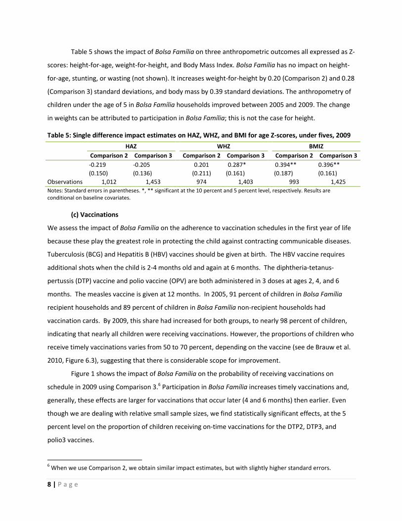
Table 5 shows the impact of Bolsa Família on three anthropometric outcomes all expressed as Z-
scores: height-for-age, weight-for-height, and Body Mass Index. Bolsa Família has no impact on height-
for-age, stunting, or wasting (not shown). It increases weight-for-height by 0.20 (Comparison 2) and 0.28
(Comparison 3) standard deviations, and body mass by 0.39 standard deviations. The anthropometry of
children under the age of 5 in Bolsa Família households improved between 2005 and 2009. The change
in weights can be attributed to participation in Bolsa Família; this is not the case for height.
Table 5: Single difference impact estimates on HAZ, WHZ, and BMI for age Z-scores, under fives, 2009
HAZ WHZ BMIZ
Comparison 2 Comparison 3 Comparison 2 Comparison 3 Comparison 2 Comparison 3
-0.219 -0.205 0.201 0.287* 0.394** 0.396**
(0.150) (0.136) (0.211) (0.161) (0.187) (0.161)
Observations 1,012 1,453 974 1,403 993 1,425
Notes: Standard errors in parentheses. *, ** significant at the 10 percent and 5 percent level, respectively. Results are conditional on baseline covariates.
(c) Vaccinations
We assess the impact of Bolsa Família on the adherence to vaccination schedules in the first year of life
because these play the greatest role in protecting the child against contracting communicable diseases.
Tuberculosis (BCG) and Hepatitis B (HBV) vaccines should be given at birth. The HBV vaccine requires
additional shots when the child is 2-4 months old and again at 6 months. The diphtheria-tetanus-
pertussis (DTP) vaccine and polio vaccine (OPV) are both administered in 3 doses at ages 2, 4, and 6
months. The measles vaccine is given at 12 months. In 2005, 91 percent of children in Bolsa Família
recipient households and 89 percent of children in Bolsa Família non-recipient households had
vaccination cards. By 2009, this share had increased for both groups, to nearly 98 percent of children,
indicating that nearly all children were receiving vaccinations. However, the proportions of children who
receive timely vaccinations varies from 50 to 70 percent, depending on the vaccine (see de Brauw et al.
2010, Figure 6.3), suggesting that there is considerable scope for improvement.
Figure 1 shows the impact of Bolsa Família on the probability of receiving vaccinations on
schedule in 2009 using Comparison 3.6 Participation in Bolsa Família increases timely vaccinations and,
generally, these effects are larger for vaccinations that occur later (4 and 6 months) then earlier. Even
though we are dealing with relative small sample sizes, we find statistically significant effects, at the 5
percent level on the proportion of children receiving on-time vaccinations for the DTP2, DTP3, and
polio3 vaccines.
6 When we use Comparison 2, we obtain similar impact estimates, but with slightly higher standard errors.

9 | P a g e
Figure 1: Single difference impact estimates of Bolsa Família on the probability of receiving vaccinations on schedule, 2009
(d) Education
Increasing education attainments is a core objective of Bolsa Família. In assessing these, it is helpful to
note patterns of enrollment in the AIBF-1 and AIBF-2 surveys. These are shown in Figures 2a and 2b. As
shown here, enrollments among children between 6 and 15 are high. So, in addition to looking at all
children, we pay particular attention to the impact on older children, those 16 and 17 who are at the
highest risk of dropping out.
Figure 2a: Proportion of children currently attending school in 2005, by age and sex
0,02 0,02
-0,12
-0,01 0,00
0,16
0,07
0,03
0,26
0,12
0,01
-0,15
-0,10
-0,05
0,00
0,05
0,10
0,15
0,20
0,25
0,30
BCG HBV1 DPT1 Polio1 HBV2 DPT2 Polio2 HBV3 DPT3 Polio3 SAR
At birth 2 months 2-4months
4 months 6 months 12months
60%
65%
70%
75%
80%
85%
90%
95%
100%
6 7 8 9 10 11 12 13 14 15 16 17
Males
Females

10 | P a g e
Figure 2b: Proportion of children currently attending school in 2009, by age and sex
Table 6 shows that Bolsa Família increases school attendance by 4.5 (Comparison 2) and 4.1
(Comparison 3) percentage points. The impact is larger for females and somewhat more precisely
measured. When we disaggregate by region, we see that these increases are concentrated in the North-
East, where enrollments rise by 16.1 (Comparison 2) and 19.9 (Comparison 3) percentage points. As the
North-East has historically lagged the rest of Brazil on many social indicators, this suggests that Bolsa
Família is contributing to the regional reductions in disparities in school attendance.
Table 6: Single difference impact estimates on the proportion of children aged 6-17 currently attending school, 2009
All children Males Females
Comparison 2 Comparison 3 Comparison 2 Comparison 3 Comparison 2 Comparison 3
0.045 0.041 0.012 0.032 0.082 0.038
(0.026) * (0.025) (0.035) (0.034) (0.033) ** (0.034)
Observations 6514 10993 3374 5633 3133 5349
Notes: Standard errors in parentheses. *, ** significant at the 10 percent and 5 percent level, respectively. Results are conditional on baseline covariates.
Rising enrollments could occur because children in school are more likely to progress to the next
grade or, rather than dropping out, children are more likely to repeat. Table 7 shows the impact of Bolsa
Família on grade progression. It shows that children aged 6-17 who reside in households receiving Bolsa
Família are more likely to progress from one grade to the next. In the Technical Appendix, we
disaggregate this result by age and sex. This shows that the impact on grade progression is concentrated
among girls aged 15 and 17 and that the effect size is large.
60%
65%
70%
75%
80%
85%
90%
95%
100%
6 7 8 9 10 11 12 13 14 15 16 17
Males
Females

11 | P a g e
Table 7: Single difference impact estimates on the proportion of children aged 6-17 in school last year that progressed to next grade level, 2009
All children Males Females
Comparison 2 Comparison 3 Comparison 2 Comparison 3 Comparison 2 Comparison 3
0.037 0.069 -0.033 0.006 0.099 0.099
(0.035) (0.033) ** (0.036) (0.039) (0.048) ** (0.048) **
Observations 4539 7703 2312 3911 2222 3786
Notes: Standard errors in parentheses. *, ** significant at the 10 percent and 5 percent level, respectively. Results are conditional on baseline covariates.
Table 8 shows the impact on repetition. There is suggestive evidence (Comparison 3, significant
at the 10 percent level) that children, particularly girls, are less likely to repeat a grade.
Table 8: Single difference impact estimates on proportion of children aged 6-17 in school last year that are repeating grade level, 2009
All children Males Females
Comparison 2 Comparison 3 Comparison 2 Comparison 3 Comparison 2 Comparison 3
-0.008 -0.050 0.057 -0.009 -0.057 -0.084
(0.032) (0.030) * (0.033) * (0.038) (0.045) (0.042) **
Observations 4539 7703 2312 3911 2222 3786
Notes: Standard errors in parentheses. *, ** significant at the 10 percent and 5 percent level, respectively. Results are conditional on baseline covariates.
(e) Child labor
Several components of the Bolsa Família program may reduce the prevalence of child labor. The most
direct effects are likely to come from the transfers that are conditioned on child schooling. In addition,
the BVJ transfer to children age 16-17 could reduce the likelihood that children in this age group drop
out of school for employment. These transfers may have significant impacts on child labor because this
is an age when it is common for children to leave school in order to work.
Levels of child labor vary by age and sex. For children aged 5-10, there is virtually no
participation in paid or unpaid work outside the home. Approximately 6 percent of children aged 11-15
work outside the home as do 16.2 and 29.3 percent of females and males aged 16 and 17, respectively.
Given these relatively low levels of participation, it is not surprising that Bolsa Família has no statistically
significant average impact on the proportion of children age 5-17 reporting doing any work in 2009.
However, of equal interest is whether Bolsa Família affects the age of entry into the labor force for
children aged 5-17. Table 9 shows that, on average, Bolsa Família delayed labor market entry by 0.8
(Comparison 2) years. The impact is larger for males than for females.

12 | P a g e
Table 9: Single difference impact estimates of Bolsa Família on age of entry into the labor force by children 5-17, 2009
All children Males Females
Comparison 2 Comparison 3 Comparison 2 Comparison 3 Comparison 2 Comparison 3
0.823 0.390 1.090 0.841 0.278 -1.062
(0.454)* (0.390) (0.740) (0.459)* (0.501) (0.614)*
Observations 245 403 156 248 88 154 Notes: Standard errors in parentheses. *, ** significant at the 10 percent and 5 percent level, respectively. Results are conditional on baseline covariates.
AIBF-2 also captured information on participation in domestic work (e.g., washing clothes,
cleaning, caring for children) and work hours in domestic activities. Bolsa Família had no impact on the
proportion of children aged 5-17 participating in any domestic work, on average, in 2009. However,
conditional on performing any domestic work, we find that Bolsa Família reduced the amount of time
girls 5-17 spent undertaking domestic work by nearly three hours per week.
4. Women’s Welfare
(a) Impact on prenatal care
Bolsa Família provides cash transfers to pregnant women to support their health during the pregnancy,
conditional on the requirement that they participate in prenatal care visits with a qualified health
professional. Information on pregnancies and prenatal care was captured in both rounds of the AIBF
survey. In the 2005 survey, the questionnaire captured whether any woman of child-bearing age in the
household was pregnant, the month of the pregnancy, and the number of prenatal care visits received.
The same information was captured in the 2009 survey.
de Brauw et al. (2010) report that in 2005, Bolsa Família recipients averaged 3.5 prenatal care
visits; this increased to 4.4 prenatal care visits by 2009. Non-recipients had only 2.9 prenatal care visits,
on average, in 2005, but had nearly caught up by 2009, with 4.3 prenatal care visits, on average. The
trend of improving utilization of prenatal care services is also clearly demonstrated by the estimates of
the proportion of pregnant women reporting receiving no prenatal care. In 2005, 20.9 percent of
women had received no prenatal care. Among Bolsa Família recipients, this share was somewhat lower,
at 17.7 percent, while 22.3 percent of pregnant women in non-recipient households had not received
any prenatal care. However, by 2009, the share of women receiving no prenatal care fell sharply to 5.7
percent and was nearly the same for Bolsa Família recipients and non-recipients. While these
descriptive trends are associations, not causal relations, they suggest that it may be difficult to find
evidence of impact.

13 | P a g e
Table 10 shows that Bolsa Família increased use of prenatal care. Bolsa recipients who were
pregnant at the time of the 2009 survey had 1.6 more prenatal care visits than pregnant women who
were non-recipients. We caution, however, that this result is based on relatively small samples of
women who were pregnant at the time of the interview in 2009.7
Table 10: Single difference impact estimates of Bolsa Família on the number of prenatal care visits, for women pregnant during the AIBF-2 survey
Comparison 2 Comparison 3
1.701 1.602
(0.913)* (0.800)**
Number of observations 75 121
Notes: Standard errors in parentheses. *, ** significant at the 10 percent and 5 percent level, respectively. Results are conditional on baseline covariates.
In light of the descriptive statistics reported above, it is not surprising that we find no evidence
that Bolsa Família reduced the proportion of pregnant women in the 2009 survey who had no prenatal
care visits. Nor do we find evidence that participation in Bolsa Família decreased the probability that a
woman's prenatal care visits were in consultation with a doctor, rather than a nurse or informal care
provider.
(b) Decisionmaking within the household
Increasing women’s decisionmaking power has both intrinsic and instrumental value: intrinsic in that
greater equity in decisionmaking is desirable in its own right; instrumental in that increasing women’s
decision-making power is seen to be associated with a series of desirable outcomes, particularly as they
relate to child welfare. Chapter 11 of de Brauw et al. (2010) describes how household decisionmaking
has evolved over time in the AIBF surveys.
In AIBF-1 and AIBF-2, respondents were asked, “In your household, generally, who makes
decisions about”: purchases of food; clothing for yourself; clothing for your spouse or partner; clothing
for children; when your child must stop attending school; health-related expenditures for children; the
purchase of consumer durables for the home; if you work or not; if your spouse works; and your
decision to use contraception. de Brauw at al. (2010) note that in most cases, the modal form of
decisionmaking is joint; joint decisionmaking is reported in 40-65 percent of the domains described
7 This small sample also means that estimates of impacts at the regional level are not very precise. However, the
relative magnitude of the estimated regional effects is still informative. Results show that the impact of Bolsa Família on the number of prenatal care visits was largest in the North and was also quite large in the North-East and South-East.
14 | P a g e
here. Second, where changes had occurred, they had been in the direction of increased decisionmaking
voice by women.
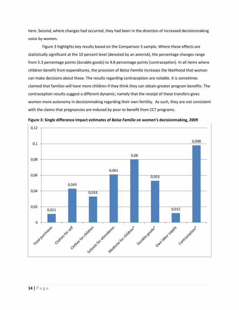
Figure 3 highlights key results based on the Comparison 3 sample. Where these effects are
statistically significant at the 10 percent level (denoted by an asterisk), the percentage changes range
from 5.3 percentage points (durable goods) to 9.8 percentage points (contraception). In all items where
children benefit from expenditures, the provision of Bolsa Família increases the likelihood that woman
can make decisions about these. The results regarding contraception are notable. It is sometimes
claimed that families will have more children if they think they can obtain greater program benefits. The
contraception results suggest a different dynamic; namely that the receipt of these transfers gives
women more autonomy in decisionmaking regarding their own fertility. As such, they are not consistent
with the claims that pregnancies are induced by poor to benefit from CCT programs.
Figure 3: Single difference impact estimates of Bolsa Família on women’s decisionmaking, 2009
0,011
0,043
0,033
0,061
0,08
0,053
0,012
0,098
0
0,02
0,04
0,06
0,08
0,1
0,12

15 | P a g e
The magnitude of these changes is large given that there are instances where the husband was
present when these answers were given. In the AIBF-1 survey, in most domains about one-sixth to one-
third of women reported making these decisions. So as a percentage change, Bolsa Família raises
women’s decisionmaking power by 29.7 and 33 percent, depending on the outcome (see Table 11
below). Regional disaggregations (found in the Technical Appendix) show that these effects tend to be
largest in the North-East and South regions.
Table 11: Magnitudes of the impact of Bolsa Família on women’s decisionmaking power
Domain Impact in percentage points
(from Comparison 2) Percentage value at
baseline Percentage change relative to baseline
(percent) (percent)
Medicine for children 8.0 24 33.0
Durable goods 5.3 17 31.2
Contraception 9.8 33 29.7
5. Household Behavior and Welfare
(a) Labor supply
A concern with any cash transfer program is that individuals in households that receive money will
reduce the number of hours they work. AIBF-1 and AIBF-2 were specifically designed to ensure that this
important issue could be addressed. Specifically, we recorded current labor force status (in the labor
force or not; in the labor force, not working but searching for work; in the labor force and working) and
the number of hours worked in a typical week for all adults aged 18-69. When we consider labor supply
in terms of hours, we do so at the household level. Specifically, we sum this across all adults and divide
by the number of individuals aged 18-69 to give a measure of household labor supply.
There is no impact of Bolsa Família on whether an individual aged 18-55 is in the labor force.
This is the case when we estimate impacts on men and women separately and when we pool the
sample. Conditional on being in the labor force, there is no statistically significant effect on the
likelihood that men work or look for work. For women, conditional on being in the labor force, Bolsa
Família weakly increases the proportion of females that have sought work among those not currently
working, by about 0.05 to 0.07, which appears driven by the North-East, where the increase is significant
and roughly 0.09 to 0.11 (depending on the use of Comparison 2 or 3). One interpretation is that receipt
of Bolsa Família makes it possible for women to search for better jobs than would be the case if they did
not receive these transfers.
Table 12 shows that there is a statistically insignificant impact on average total household
weekly work hours among individuals aged 18-69 per individual aged 18-69. Disaggregated by region,

16 | P a g e
there is an insignificant impact in all regions.
Table 12: Impact on average household weekly work hours
Among all members aged 18-69, per member aged 18-69
Among males aged 18-69, per male aged 18-69
Among females aged 18-69, per female aged 18-69
Comparison 2 Comparison 3 Comparison 2 Comparison 3 Comparison 2 Comparison 3
0.166 -0.110 -0.785 -0.384 0.304 0.244
(1.146) (0.949) (1.599) (1.336) (1.495) (1.344)
Observations 3661 5391 3432 5078 3410 5066 Notes: Standard errors in parentheses. *, ** significant at the 10 percent and 5 percent level, respectively. Results are conditional on baseline covariates.
We can also see whether the type of work changed. AIBF-1 and AIBF-2 contain information that
allow us to characterize each job worked by a household member as being in the formal sector or
informal sector. We define a job as being in the formal sector if the household member either has a
“card” for that job or contributes to social security through that job. 8 Overall, conditional on baseline
covariates, there is a significant decrease in average formal household weekly work hours among
individuals aged 18-69 per individual aged 18-69, by roughly eight hours. By contrast, conditional on
baseline covariates, there is a significant increase in average informal household weekly work hours
among individuals aged 18-69 per individual aged 18-69, by roughly eight hours, suggesting that there is
indeed a shift across sectors.9
When we disaggregate by sex, we find a significant decrease in average formal household
weekly work hours among males aged 18-69 per male aged 18-69, by roughly 4.6 hours (Comparison 2
and 3, statistically significant at the 5 percent level). This is driven by impacts observed in the North and
North-East. By contrast, conditional on baseline covariates, there is a significant increase in average
informal household weekly work hours among males aged 18-69 per male aged 18-69, by roughly 5.3
hours (Comparisons 2 and 3, statistically significant at the 5 percent level). Disaggregated by region,
there is an increase in average informal household weekly work hours among males in the North-East by
3.4 – 4.2 hours (Comparisons 2 and 3 respectively, statistically significant at the 5 percent level). Among
women, conditional on baseline covariates, there is a decrease in average formal household weekly
work hours of 4.1 hours among females aged 18-69 per female aged 18-69 based on Comparison 2. This
appears to be driven by an increase in informal sector work by women in the North-East.
8 These results are based in Comparison 2. Results using Comparison 3 are very similar.
9 A caveat to this finding is that some differences appear to exist in formal-sector work and informal-sector work
between our Comparison 2 treatment and control groups even at baseline.

17 | P a g e
Given these results, we ask to what extent the proportion of work shifted between the formal
and informal sector and to what extent has it shifted within the household. Conditional on baseline
covariates, we find a statistically significant decrease in the proportion of total household weekly work
hours devoted to the formal sector by roughly 20 percent when using either Comparison 2 or
Comparison 3. This impact is statistically significant at the 5 percent level. This switch from the formal to
informal sector is most marked in the North-East, where the proportion of total household weekly work
hours devoted to the formal sector falls by roughly 22 percent based on Comparison 2. By contrast,
there is an insignificant impact in the proportion of total household weekly work hours worked by
females.
There are several possible explanations for the differences we observe in formal- and informal-
sector work. Bolsa Família Program has adopted administrative procedures to cross-check households’
self-reported incomes; however, these procedures are only possible when at least one member of the
household is working in the formal sector. One explanation for our findings is that this procedure
created an incentive to hide income through informal work, and some Bolsa Família beneficiaries were
induced to switch from the formal sector to the informal sector. A second possibility is that, due to the
administrative cross-checks, a disproportionate share of households already working in the formal
sector were excluded from the program between our baseline and follow-up surveys, leading formal-
sector workers to be underrepresented among beneficiaries at follow-up. A third explanation is that,
among potential beneficiaries, workers with a more unstable trajectory in the labor market tended to
prefer work in the informal sector with access to steady benefits, while workers with a more stable
trajectory preferred to work in the typically-higher-paying formal sector even with the risk of losing the
benefits. While our data do not allow us to readily distinguish between these explanations, all three
may play some role.
(b) Social capital
In de Brauw et al. (2010), we noted that the level of participation in groups and networks was relatively
low. Mindful of this, we estimated the effect of Bolsa Família on group participation. There is weak
evidence that Bolsa increases group membership, but this is dependent on how membership is defined,
the specific method of estimating impact used and the location of the recipient.
6. Summary

18 | P a g e
Using propensity score weighting, we have examined the impact of Bolsa Família on the welfare of
children, mothers, and households. Bolsa Família improves welfare in the following ways:
- It increases the likelihood that children are born full-term, although this effect is imprecisely
measured;
- It improves certain dimensions of children’s anthropometry: their weight-for-height and body
mass;
- There are statistically significant effects on the proportion of children receiving on-time DTP2,
DTP3 and polio3 vaccines. These effects are large in magnitude;
- Bolsa Família increases school attendance by 4.5 (Comparison 2) and 4.1 (Comparison 3)
percentage points. The impact is larger for females. These increases are concentrated in the
North-East;
- Children in households receiving Bolsa Família are more likely to progress from one grade to the
next. This impact is largest among girls aged 15 and 17 and that the effect size is large;
- There is some evidence that Bolsa Família children, particularly girls, are less likely to repeat a
grade. However, these effects are imprecisely measured.
- Complementary to the schooling results, Bolsa Família delays children’s labor market entry by
about one year although this is imprecisely measured;
- Bolsa Família had no impact on the proportion of children aged 5-17 participating in any
domestic work, on average, in 2009. However, conditional on performing any domestic work,
we find that Bolsa Família reduced the amount of time girls 5-17 spent undertaking domestic
work by nearly three hours per week;
- Pregnant women in households receiving Bolsa Família transfers receive, have 1.6 more
prenatal visits with a health care professional; and
- In all items where children benefit from expenditures, the provision of Bolsa Família increases
the likelihood that woman can make decisions about these with the largest impact found on
contraceptive choice. It is sometimes claimed that families will have more children if they think
they can obtain greater program benefits. The contraception results suggest a different
dynamic; namely that the receipt of these transfers gives women more autonomy in
decisionmaking regarding their own fertility. As such, they are not consistent with the claims
that pregnancies are induced by poor to benefit from CCT programs.

19 | P a g e
- There is no meaningful evidence that Bolsa Família reduces labor supply. There is some
evidence that in participant households, men have been working fewer hours per week in the
formal sector and more hours in the informal sector.
References
de Brauw, A., D. Gilligan, J. Hoddinott, V. Moreira and S. Roy, 2010. Bolsa Família: Descriptive Statistics from AIBF-1 and AIBF-2, International Food Policy Research Institute: Washington DC.
Hirano, K, G. Imbens, and G. Ridder, 2003. Efficient estimation of average treatment effects using the estimated propensity score, Econometrica 71: 1161-1189.
WHO (World Health Organization), 2006. WHO Child Growth Standards: Length/Height-for-Age, Weight-
for-Age, Weight-for-Length, Weight-for-Height and Body Mass Index-for-Age: Methods and
Development, World Health Organization, Geneva.

The Impact of Bolsa Família on Child, Maternal, and Household Welfare
Technical Appendix

22 | P a g e
Contents Section 1. Estimation Methodology ........................................................................................................... 23
1.1 Overview of propensity score weighting .......................................................................................... 23
1.2 Theoretical basis for propensity score weighting ............................................................................. 24
1.3 Implementation of propensity score weighting ............................................................................... 26
1.3.1 Selection of potential comparison groups ............................................................................... 26
1.3.2 Estimating propensity scores ................................................................................................... 27
1.3.3 Assessing similarity of each treatment and comparison group, per estimated
propensity scores .................................................................................................................... 29
1.3.4 Assessing balancing of observables using propensity score weights....................................... 31
1.3.5 Accounting for high variance ................................................................................................... 33
Section 2. Full Set of Impact Estimates ....................................................................................................... 35
2.1 Children’s welfare ............................................................................................................................. 35
2.1.1 Birthweight ............................................................................................................................... 35
2.1.2 Anthropometry ........................................................................................................................ 39
2.1.3 Vaccinations ............................................................................................................................. 41
2.1.4 Education.................................................................................................................................. 42
2.1.5 Child labor ................................................................................................................................ 55
2.2 Women’s welfare .............................................................................................................................. 59
2.2.1 Impact on prenatal care ........................................................................................................... 59
2.2.2 Decisionmaking within the household ..................................................................................... 63
2.3 Household behavior and welfare ...................................................................................................... 67
2.3.1 Labor supply ............................................................................................................................. 67
2.3.2 Social capital ............................................................................................................................. 79
References .................................................................................................................................................. 81

23 | P a g e
Section 1. Estimation Methodology
1.1 Overview of propensity score weighting
In this appendix, we describe in more detail the methodology we use to estimate the impacts of Bolsa
Família. We wish to estimate average treatment impacts on the treated (ATT): that is, the impact that
Bolsa Família had on a range of outcomes for recipients, using non-recipients as a proxy for what their
outcomes would have counterfactually been in the absence of Bolsa Família. The key challenge in
evaluating these impacts, for a nonrandomly assigned program such as Bolsa Família, is accounting for
characteristics that may be correlated both with receipt of the program and with outcomes of interest
conditional on program receipt. If program recipients differ systematically from non-recipients, even
preprogram, in ways that may also affect our outcomes of interest, we must take these differences into
account in order to avoid biased impact estimates.
The Bolsa Família Program is targeted at poor households. Consequently, program recipients
tend to look quite different from non-recipients, even preprogram. In evaluating Bolsa Família, we
therefore turn to impact estimation methodologies designed for nonrandom program assignment. Our
preferred methodology for this evaluation is propensity score weighting (Hirano, Imbens, and Ridder
2003), an approach that entails estimating and applying weights to statistically balance preprogram
characteristics between Bolsa Família recipients and the specific selection of non-recipients we use for
comparison.
As discussed in the main report, the basic intuition behind the propensity score weighting
estimator is as follows. We first estimate a propensity score for each household, which indicates the
predicted probability that the household is a Bolsa Família recipient rather than in a comparison group
of non-recipients, based on a range of observable preprogram characteristics. We then use the
propensity scores to place weights on the comparison observations. These weights adjust for the fact
that some households in the comparison group do not have high predicted probability of being Bolsa
Família recipients based on their observable characteristics; these households receive low weights in the
estimation of ATT. Meanwhile, other households in the control group have observable characteristics
very similar to households receiving Bolsa Família payments; these households are assigned higher
weights. Intuitively, by placing higher weights on non-recipient households that have characteristics
more like recipients and lower weights on non-recipient households that have characteristics less like
recipients, we balance observable characteristics between recipients and non-recipients, even if they
were unbalanced before weighting. Hirano, Imbens, and Ridder (2003) show that, under assumptions
described below, applying the propensity score weights leads to unbiased impact estimates of ATT.

24 | P a g e
There are two key criteria that lead us to choose propensity score weighting as our preferred
methodology for estimating the impacts of Bolsa Família. First, unlike other standard methodologies for
impact estimation in nonrandomized settings, propensity score weighting allows us to take into account
the sampling weights and attrition weights in our data. Incorporating these weights allows us to
interpret our estimates of ATT as representative of the treated population, adjusting for oversampling of
certain types of households in the baseline and selective attrition of certain types of households in the
follow-up. Second, the methodology imposes a relatively smaller computational burden than alternative
estimators for nonrandomized settings. For a dataset with such large sample size, use of more time-
consuming procedures (such as covariate matching) would limit the feasibility of estimating impacts on a
rich set of outcomes. The main disadvantage of using propensity score weighting as opposed to
matching methods is the higher variance of the estimator (Freedman and Berk 2008). We describe
below the measures we take to, first, reduce variance to the extent possible, and second, use alternative
methods as robustness checks when impacts using propensity score weighting are borderline-significant.
1.2 Theoretical basis for propensity score weighting
We present here a brief overview of the theoretical basis for propensity score weighting, based on
Hirano, Imbens, and Ridder (2003).
The aim of our evaluation is to construct, for a range of outcomes, an estimate of the average
impact of Bolsa Família on those that receive it—referred to as the average impact of the treatment on
the treated (ATT). The formalization of this concept is as follows.
Let Yt1 be a household’s outcome in time period t if it is a recipient of Bolsa Família, let Yt
0 be
that household’s outcome in time period t if it does not receive any program benefits, and let D be an
indicator variable equal to 1 if the household receives program benefits and 0 if not (i.e., an indicator of
“treatment”). The impact of the program is just the change in the outcome caused by receiving benefits:
Δ = Yt1 - Yt
0. For each household, either only Yt1 or only Yt
0 is observed in any period t.
We wish to estimate the difference between the outcome that treated households would realize
if they receive the program and the outcome that treated households would realize if they do not
receive the program in period t, given a vector X of observable characteristics of the households:
ATT = E(Δ | X,D = 1) = E(Yt1 - Yt
0 | X,D = 1) = E(Yt1 | X,D = 1) - E(Yt
0 | X,D = 1).
However, only Yt1 and not Yt
0 is observed for households treated in period t, i.e., those with
D = 1. Because E(Yt0 | X,D = 1) is not observed, we must construct a statistical comparison group for
recipients out of our observations on non-recipients, i.e., households with D = 0. In particular, we must

25 | P a g e
construct a group of non-recipients and then adjust it in such a way that balances any observable
characteristics X potentially correlated both with treatment status and the outcome conditional on
treatment status.
One way of doing so involves estimating a “propensity score,” P(X) = Pr(D = 1 | X). This
propensity score is the predicted probability that any household is a program recipient based only on its
observable characteristics X. The approach of propensity weighted regression entails the researcher
selecting a set of non-recipients to use as a comparison group, then using estimated propensity scores
for program receipt to more heavily weight the comparison observations with higher propensity
scores.10 The validity of this approach rests in part on two assumptions:
E(Yt0 | X,D = 1) = E(Yt
0 | X,D = 0), (A1)
and
0 < P(X) < 1. (A2)
Expression (A1) assumes “conditional mean independence”, i.e., that conditional on X,
nonparticipants have the same mean outcomes as participants would have if they did not receive the
program. Expression (A2) assumes that, based only on the set of observables X, all observations in the
comparison group have positive predicted probability of being treated.
We first consider the case without sampling or attrition weights.
Under (A1), (A2), and several other technical assumptions, Hirano, Imbens, and Ridder show
that we obtain an unbiased estimate of ATT through a weighted regression framework, if the ratio of
assigned weights is )(1
)(
XP
XP
:1 for comparison : treatment observations . 11
10
We describe below in Section 1.3 how, in practice, we define possible comparison groups and how we estimate propensity scores. 11
Note that this approach differs from matching methods, in that for matching, only certain observations out of the eligible comparison group are used—based on some metric of similarity to treated observations, depending on the particular method—but that typically each of those observations is then assigned a weight of 1. In propensity score weighting, all observations in the comparison group selected by the researcher are used, but each is assigned a weight based on its propensity score. (This approach is preferable for our context, since incorporating sample weights and attrition weights is then relatively straightforward.) In this respect, the researcher’s selection of the comparison group is quite important for propensity score weighting, since all observations are used with nonzero weight. We discuss our selection of possible comparison groups for this evaluation in the main report and demonstrate their comparability in Section 1.3.3 of this appendix.
26 | P a g e
Hirano, Imbens, and Ridder also show that the observables X used to construct the propensity
score can be directly included in this weighted regression to account for additional variation and thereby
improve precision. 12
It is straightforward to extend this methodology to the case where, as in this evaluation, there
are also sampling weights and attrition weights. These weights can simply be multiplied to the
propensity-score weights to derive an “effective weight” to be used in the weighted regression.
1.3 Implementation of propensity score weighting
As described above, there are two ways by which we adjust for differences in observable characteristics
between the Bolsa Família recipients and non-recipients that we compare: (1) select a comparison
group of non-recipients that, in the first place, is likely to be fairly similar to the treated group of
recipients in terms of observable characteristics, and (2) use estimated propensity scores to weight each
observation in the comparison group according to its similarity to treated observations. We assess the
first by looking at overlap in estimated propensity scores between each treatment and comparison
group. We assess the second by looking at the extent to which a set of observable characteristics is
balanced between each treatment and comparison group once the propensity score weights are taken
into account.
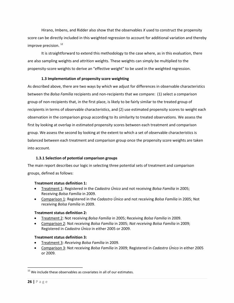
1.3.1 Selection of potential comparison groups
The main report describes our logic in selecting three potential sets of treatment and comparison
groups, defined as follows:
Treatment status definition 1:
Treatment 1: Registered in the Cadastro Único and not receiving Bolsa Família in 2005; Receiving Bolsa Família in 2009.
Comparison 1: Registered in the Cadastro Único and not receiving Bolsa Família in 2005; Not receiving Bolsa Família in 2009.
Treatment status definition 2:
Treatment 2: Not receiving Bolsa Família in 2005; Receiving Bolsa Família in 2009.
Comparison 2: Not receiving Bolsa Família in 2005; Not receiving Bolsa Família in 2009; Registered in Cadastro Único in either 2005 or 2009.
Treatment status definition 3:
Treatment 3: Receiving Bolsa Família in 2009.
Comparison 3: Not receiving Bolsa Família in 2009; Registered in Cadastro Único in either 2005 or 2009.
12
We include these observables as covariates in all of our estimates.

27 | P a g e
Based on sample size considerations, particularly for disaggregations by age, sex, and region, we
focus on presenting results only for Treatment status definition 2 (denoted as simply “Comparison 2”)
and Treatment status definition 3 (denoted as simply “Comparison 3”).
1.3.2 Estimating propensity scores
Using propensity score weighting requires choosing a method for estimating propensity scores. Ideally,
we wish to include all observable characteristics in the propensity score that are correlated both with
the probability of receiving Bolsa Família and with outcomes related to Bolsa Família conditional on
receipt status. We also would like to let the data tell us the relationship between the probability of
treatment and these observable characteristics. In other words, we prefer to allow for as flexible a
relationship as possible, rather than imposing a particular functional form. These considerations are
taken into account in the approach described here.
We start by selecting a large set of observable preprogram characteristics that we perceive as
having potential to be correlated with both program receipt and our outcomes of interest conditional on
program receipt status.13 This set of observables includes characteristics both at the household level and
at the municipality level.
To then estimate propensity scores, we follow the following stepwise algorithm, which in
essence follows Hirano, Imbens, and Ridder (2003). We start by estimating a logit model including only
region dummy variables interacted with rural-urban dummies, to ensure that we account for broad
differences in market conditions. We weight the regression by sampling weights from the AIBF-1 data
multiplied by attrition weights. Next, we start to consider the set of N variables at the household and
municipality level as possible covariates for inclusion in the logit model. We estimate N regressions, each
sequentially and separately including one variable to the basic logit model. We keep the variable that
reduces the log pseudo-likelihood the most. We then take the remaining list of N-1 variables, and
sequentially add the remaining N-1 variables to the logit model, again keeping the one that maximizes
the reduction of the log pseudo-likelihood. We follow this procedure until the reduction hits a threshold
that roughly corresponds to adding a variable to the logit model that has a t-ratio of 1, indicating that
the remaining variables in the list have little predictive power.14
13
In the case of Comparison 3, since some in the treatment group are already receiving Bolsa Familia at baseline, we allow inclusion of only characteristics that are unlikely to be affected by already receiving treatment. 14
We use the list of predictive explanatory variables for any regressions using covariate matching, when we run robustness checks. Since covariate matching does not parameterize the relationship between explanatory variables and treatment status, we do not need to include any second order terms.

28 | P a g e
We next take the K covariates that are chosen in the first step, and in the second step we square
all of them and interact them with one another, creating an additional K(K + 1)/2 variables. We then add
these second order terms to the model sequentially until no term exceeds a threshold that loosely
indicates significant predictive power (e.g., a t-ratio that corresponds to a p-value of 0.1). We repeat this
procedure for each of the three comparisons, therefore letting the data tell us the relationship between
Bolsa Família eligibility and potential explanatory variables.
Table A1 shows the full set of covariates we allow to enter our constructed propensity scores.
The table also indicates which covariates enter estimated propensity scores for each comparison group,
following the algorithm described above.

29 | P a g e
Table A1: Household- and municipality-level characteristics included as possible covariates for propensity score estimates
Covariate in Comparison
Level Variable Year 1a 2
a 3
a
Household (from AIBF) Number of children aged 0-15 at baseline 2005 X X X
Household (from AIBF) Household size 2005 X X
Household (from AIBF) Number of rooms in house (truncated at 10) 2005 X
Household (from AIBF) Number of bedrooms in house 2005
Household (from AIBF) Number of bathrooms in house 2005
Household (from AIBF) Housing quality index, from 0-11 2005 X X X
Household (from AIBF) Whether household owns its house 2005
Household (from AIBF) Log of per-capita monthly expenditure (food + nonfood) 2005 X X b
Household (from AIBF) Whether head is illiterate 2005 X
Household (from AIBF) Head’s years of education 2005 X
Household (from AIBF) Head’s sex 2005
Municipality Average family size 2000 X X
Municipality Child dependency ratio 2000 X X
Municipality Incidence of poverty 2003 X
Municipality Incidence of extreme poverty 2003 X
Municipality Percent of population working without card 2000 X X
Municipality Percent of population working in agricultural sector 2000 X X
Municipality Black population, as percentage of total population 2000 X
Municipality “Pardo” population, as percentage of total population 2000 X
Municipality Indigenous population, as percentage of total population 2000
Municipality Percent of households with “adequate housing” 2000
Municipality Percent of households with access to piped water 2000 X X
Municipality Percent of households with access to solid waste collection 2000 X X
Municipality Percent of households with access to general sewage network 2000
Municipality Percent of households with access to septic tanks 2000 X
Municipality Percent of households with access to electricity 2003
Municipality Households with landline phones (per 1,000) 2000
Municipality Households with cell phones (per 1,000) 2000 X
Municipality Average years of education 2000
Municipality School attendance rate: 7-14 y.o. 2000 X X X
Municipality Illiteracy rate: 7 to 14 y.o. 2003
Municipality Number of public schools per capita 2003 X X
Municipality Average number of students per class in elementary school 2003 X
Municipality Number of clinics (“postos medicos”) per thousand inhabitants 2002 x a All comparisons include as covariates the interactions of region and rural/urban dummies.
b Excluded from consideration.
1.3.3 Assessing similarity of each treatment and comparison group, per estimated propensity scores
Based on the algorithm above, we estimate propensity scores over the set of listed covariates for each
of the three comparisons defined. Below we graph kernel densities to compare the distribution of
estimated propensity scores among recipients vs. the distribution of estimated propensity scores among
non-recipients, for each of the three comparison definitions (Figures A1-A3). If the two distributions did

30 | P a g e
not largely overlap one another, we would be concerned that the treatment and comparison groups we
had defined were not comparable along observable characteristics. However, in each case we find very
good overlap, suggesting that we can have confidence that the estimated propensity scores will help
correct imbalances between the two groups.
Figure A.1 Overlap in propensity scores for comparison between Bolsa Família recipients and non-recipients, using Comparison Definition 1
Figure A2: Overlap in propensity scores for comparison between Bolsa Família recipients and non-recipients, using Comparison Definition 2
0
.5
1
1.5
0 .2 .4 .6 .8 1 Comparison One
Non-Recipients Recipients
Kernel density of propensity scores, by recipient status

31 | P a g e
Figure A3: Overlap in propensity scores for comparison between Bolsa Família recipients and non-recipients, using Comparison Definition 3
1.3.4 Assessing balancing of observables using propensity score weights
To assess how well weights based on these estimated propensity scores balance observable
characteristics between each treatment and comparison group, we test for average differences in those
characteristics between the groups after applying the propensity score weights to the comparison
group.
Tables A2 and A3 show the unweighted means and the weighted means for the treatment and
comparison groups in Comparison 2 and Comparison 3 (as mentioned above, we do not present
estimates from Comparison 1 due to small sample sizes). Before we use the propensity weights, we find
statistically significant differences for many of the characteristics. After the propensity weights are
applied, in both comparisons the average differences are no longer statistically significant. Therefore we
can comfortably state that the propensity scores appear to account for significant differences between
the groups of recipients and non-recipients for both comparisons.

32 | P a g e
Table A2: Comparison 2—Balancing of covariates, unweighted and weighted
Variable
Included in
construction
of p-score
Unweighted means Weighted means p-value on
difference in
weighted
means Control Treatment Control Treatment
HH: Number of children age 0-15 at baseline X 1.42 2.10 1.72 1.68 0.71
HH: Household size X 4.20 4.77 4.03 4.01 0.89
HH: Number of rooms in house 5.18 4.88 5.06 5.07 0.96
HH: Number of bedrooms in house 0.27 0.34 0.25 0.22 0.56
HH: Number of bathrooms in house 0.89 0.77 0.83 0.86 0.54
HH: Housing quality index, from 0-11 X 8.25 7.57 7.59 7.83 0.22
HH: Whether household owns its house 0.67 0.67 0.68 0.63 0.26
HH: Log of per-capita monthly expenditures X 5.20 4.96 5.01 5.10 0.18
HH: Whether head is illiterate X 0.22 0.25 0.24 0.24 0.99
HH: Head’s years of education 3.49 3.52 3.51 3.57 0.82
HH: Head’s sex 0.36 0.36 0.37 0.38 0.79
Muni: Average family size X 3.60 3.69 3.58 3.57 0.80
Muni: Child Dependency Ratio 49.49 52.34 49.87 49.55 0.60
Muni: Incidence of poverty 39.29 45.74 43.68 42.98 0.66
Muni: Incidence of extreme poverty 0.13 0.16 0.14 0.14 0.51
Muni: Percent without card X 39.64 43.54 42.99 43.43 0.78
Muni: Percent in agricultural sector X 23.69 27.63 28.23 28.64 0.80
Muni: Percent black 6.51 6.69 7.59 7.15 0.29
Muni: Percent “pardo” 46.95 51.94 48.42 46.67 0.40
Muni: Percent indigenous 0.38 0.42 0.43 0.49 0.26
Muni: Percent with “adequate housing” 34.98 28.67 33.41 34.03 0.71
Muni: Percent with piped water X 69.70 64.79 68.09 68.56 0.71
Muni: Percent with solid waste collection X 71.24 64.64 67.17 67.31 0.94
Muni: Percent with general sewage network 38.56 30.15 37.43 38.74 0.53
Muni: Percent with septic tanks 14.28 14.71 12.79 12.09 0.56
Muni: Percent with electricity 91.09 88.57 90.06 91.13 0.16
Muni: Landline phones (per 1,000) 246.47 220.58 240.90 244.13 0.62
Muni: Cell phones (per 1,000) X 146.18 131.30 140.03 143.73 0.52
Muni: Average years of education 5.57 5.24 5.15 5.17 0.82
Muni: School attendance rate: 7-14 y.o. X 94.51 93.77 93.40 93.57 0.70
Muni: Illiteracy rate: 7 to 14 y.o. 12.77 15.64 14.22 13.55 0.38
Muni: Number of public schools per capita X 0.001 0.001 0.001 0.001 0.94
Muni: Number of students per elementary class 28.22 28.00 27.59 27.50 0.68
Muni: Clinics (per 1,000) 2.04 1.80 1.66 1.63 0.81
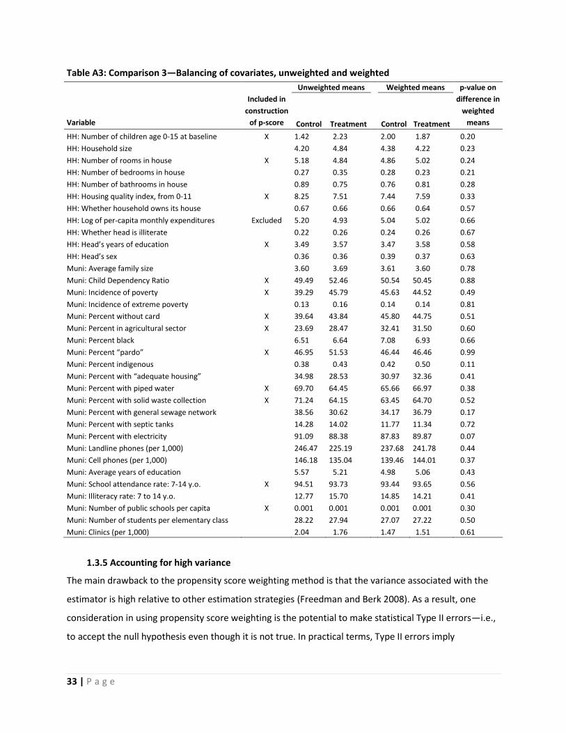
33 | P a g e
Table A3: Comparison 3—Balancing of covariates, unweighted and weighted
Variable
Included in
construction
of p-score
Unweighted means Weighted means p-value on
difference in
weighted
means Control Treatment Control Treatment
HH: Number of children age 0-15 at baseline X 1.42 2.23 2.00 1.87 0.20
HH: Household size 4.20 4.84 4.38 4.22 0.23
HH: Number of rooms in house X 5.18 4.84 4.86 5.02 0.24
HH: Number of bedrooms in house 0.27 0.35 0.28 0.23 0.21
HH: Number of bathrooms in house 0.89 0.75 0.76 0.81 0.28
HH: Housing quality index, from 0-11 X 8.25 7.51 7.44 7.59 0.33
HH: Whether household owns its house 0.67 0.66 0.66 0.64 0.57
HH: Log of per-capita monthly expenditures Excluded 5.20 4.93 5.04 5.02 0.66
HH: Whether head is illiterate 0.22 0.26 0.24 0.26 0.67
HH: Head’s years of education X 3.49 3.57 3.47 3.58 0.58
HH: Head’s sex 0.36 0.36 0.39 0.37 0.63
Muni: Average family size 3.60 3.69 3.61 3.60 0.78
Muni: Child Dependency Ratio X 49.49 52.46 50.54 50.45 0.88
Muni: Incidence of poverty X 39.29 45.79 45.63 44.52 0.49
Muni: Incidence of extreme poverty 0.13 0.16 0.14 0.14 0.81
Muni: Percent without card X 39.64 43.84 45.80 44.75 0.51
Muni: Percent in agricultural sector X 23.69 28.47 32.41 31.50 0.60
Muni: Percent black 6.51 6.64 7.08 6.93 0.66
Muni: Percent “pardo” X 46.95 51.53 46.44 46.46 0.99
Muni: Percent indigenous 0.38 0.43 0.42 0.50 0.11
Muni: Percent with “adequate housing” 34.98 28.53 30.97 32.36 0.41
Muni: Percent with piped water X 69.70 64.45 65.66 66.97 0.38
Muni: Percent with solid waste collection X 71.24 64.15 63.45 64.70 0.52
Muni: Percent with general sewage network 38.56 30.62 34.17 36.79 0.17
Muni: Percent with septic tanks 14.28 14.02 11.77 11.34 0.72
Muni: Percent with electricity 91.09 88.38 87.83 89.87 0.07
Muni: Landline phones (per 1,000) 246.47 225.19 237.68 241.78 0.44
Muni: Cell phones (per 1,000) 146.18 135.04 139.46 144.01 0.37
Muni: Average years of education 5.57 5.21 4.98 5.06 0.43
Muni: School attendance rate: 7-14 y.o. X 94.51 93.73 93.44 93.65 0.56
Muni: Illiteracy rate: 7 to 14 y.o. 12.77 15.70 14.85 14.21 0.41
Muni: Number of public schools per capita X 0.001 0.001 0.001 0.001 0.30
Muni: Number of students per elementary class 28.22 27.94 27.07 27.22 0.50
Muni: Clinics (per 1,000) 2.04 1.76 1.47 1.51 0.61
1.3.5 Accounting for high variance
The main drawback to the propensity score weighting method is that the variance associated with the
estimator is high relative to other estimation strategies (Freedman and Berk 2008). As a result, one
consideration in using propensity score weighting is the potential to make statistical Type II errors—i.e.,
to accept the null hypothesis even though it is not true. In practical terms, Type II errors imply

34 | P a g e
potentially missing significant impacts of Bolsa Família, leading us to take two specific measures to deal
with high variance.
First, to the extent possible, we lower the variance of the propensity score weighting estimator
by including the covariates used to estimate the propensity score directly in all our weighted regressions
estimating treatment effects. As mentioned above, these variables should no longer affect the point
estimate of the treatment effect after propensity score weighting, but act only to improve its precision.
Second, when we find impact estimates that are borderline significant (i.e., statistically
significant between the 5-10 percent level) even after adding covariates, we attempt to also estimate
them via nearest neighbor matching, also known as “covariate matching” (Abadie and Imbens 2006) and
confirm that results are significant. Covariate matching compares outcomes among treated observations
with outcomes among selected observations in the comparison group for which a set of explanatory
variables is closest to the treated observation, according to a distance measure. The estimated
treatment effect is the average difference for the outcome between the treatment and “nearest
neighbor” comparison observations. An advantage to using covariate matching is that it is a lower
variance estimation strategy relative to propensity score weighting. Covariate matching is also entirely
nonparametric and does not rely on the distributional assumptions that underlie the probit or logit
model used to estimate propensity scores in propensity score weighting. However, covariate matching
does not allow us to readily take into account sample weights and attrition weights, such that we would
expect slight differences between the point estimates of impacts based on propensity score weighting
vs. covariate matching. Moreover, covariate matching is very computationally intensive in large samples
and therefore, for a dataset as large as our Bolsa Família study sample, is more suitable to use as a
robustness check for borderline-significant results than as our primary estimation strategy.

35 | P a g e
Section 2. Full Set of Impact Estimates
Note that, for all tables below, significance levels are denoted as follows:
* Significant at the 10 percent level, ** significant at the 5 percent level, *** significant at the 1 percent
level.
2.1 Children’s welfare
2.1.1 Birthweight
We consider the following outcomes related to infant health: mean birthweight in kilograms (Tables
A4-A6), proportion of low-birthweight children (Tables A7-A9), proportion of children born full-term
(Tables A10-A12), proportion of children ever breastfed (Tables A13-A15), and proportion of children
breastfed exclusively for six or more months (Tables A16-A18).
In general, there are very few significant impacts, although sample sizes are too small to
interpret the results conclusively as there being no impact. Among all the outcomes considered, impact
coefficients on proportion of children born full-term are also mixed but tend to be either positive and
significant or positive and insignificant. Among girls, both Comparison 2 and Comparison 3 suggest
significant positive impacts.
Table A4: Impact of Bolsa Família on mean birthweight (in kg) among children aged 0-1 in 2009
Comparison 2 Comparison 3
Overall, conditional on baseline covariates 0.022 0.026
(0.072) (0.068)
Observations 361 561
Regional mean impacts (unconditioned) North -0.483 -0.379
(0.203) ** (0.162) **
North-East -0.091 -0.175
(0.134) (0.145)
South-East 0.128 0.447
(0.227) (0.329)
South -0.011 -0.095
(0.060) (0.097)
Centre-West 0.494 0.439
(0.260) * (0.248) *
Observations 372 574
Table A5: Impact of Bolsa Família on mean birthweight (in kg) among boys aged 0-1 in 2009
Comparison 2 Comparison 3
Overall, conditional on baseline covariates 0.061 0.097
(0.075) (0.092)
Observations 184 273
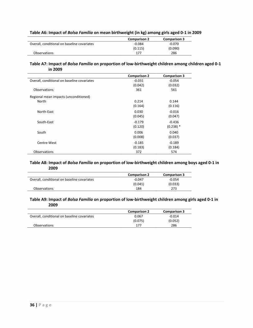
36 | P a g e
Table A6: Impact of Bolsa Família on mean birthweight (in kg) among girls aged 0-1 in 2009
Comparison 2 Comparison 3
Overall, conditional on baseline covariates -0.084 -0.070
(0.115) (0.090)
Observations 177 286
Table A7: Impact of Bolsa Família on proportion of low-birthweight children among children aged 0-1
in 2009
Comparison 2 Comparison 3
Overall, conditional on baseline covariates -0.031 -0.054
(0.042) (0.032)
Observations 361 561
Regional mean impacts (unconditioned) North 0.214 0.144
(0.164) (0.116)
North-East 0.030 -0.016
(0.045) (0.047)
South-East -0.179 -0.436
(0.120) (0.238) *
South 0.006 0.040
(0.008) (0.037)
Centre-West -0.185 -0.189
(0.183) (0.184)
Observations 372 574
Table A8: Impact of Bolsa Família on proportion of low-birthweight children among boys aged 0-1 in
2009
Comparison 2 Comparison 3
Overall, conditional on baseline covariates -0.047 -0.054
(0.041) (0.033)
Observations 184 273
Table A9: Impact of Bolsa Família on proportion of low-birthweight children among girls aged 0-1 in
2009
Comparison 2 Comparison 3
Overall, conditional on baseline covariates 0.067 -0.014
(0.075) (0.052)
Observations 177 286

37 | P a g e
Table A10: Impact of Bolsa Família on proportion of children born full-term among children aged 0-1 in 2009
Comparison 2 Comparison 3
Overall, conditional on baseline covariates 0.107 0.079
(0.060) * (0.053)
Observations 411 629
Regional mean impacts (unconditioned) North -0.001 -0.001
(0.011) (0.009)
North-East 0.245 0.066
(0.142) * (0.061)
South-East 0.111 0.343
(0.126) (0.251)
South -0.021 -0.112
(0.023) (0.070)
Centre-West 0.090 0.044
(0.141) (0.193)
Observations 422 642
Table A11: Impact of Bolsa Família on proportion of children born full-term among boys aged 0-1 in
2009
Comparison 2 Comparison 3
Overall, conditional on baseline covariates 0.068 -0.025
(0.055) (0.042)
Observations 208 305
Table A12: Impact of Bolsa Família on proportion of children born full-term among girls aged 0-1 in
2009
Comparison 2 Comparison 3
Overall, conditional on baseline covariates 0.158 0.148
(0.087) * (0.069) **
Observations 187 322
Table A13: Impact of Bolsa Família on proportion of children ever breastfed among children aged 0-1
in 2009
Comparison 2 Comparison 3
Overall, conditional on baseline covariates -0.012 -0.019
(0.031) (0.027)
Observations 392 643
Regional mean impacts (unconditioned) North 0.000 -0.011
(0.000) (0.011)
North-East -0.024 -0.021
(0.041) (0.033)
South-East -0.446 -0.347
(0.256) * (0.229)
South -0.041 -0.037
(0.049) (0.035)
Centre-West 0.254 0.097
(0.209) (0.097)
Observations 429 656

38 | P a g e
Table A14: Impact of Bolsa Família on proportion of children ever breastfed among boys aged 0-1 in
2009
Comparison 2 Comparison 3
Overall, conditional on baseline covariates -0.021 -0.003
(0.052) (0.040)
Observations 217 316
Table A15: Impact of Bolsa Família on proportion of children ever breastfed among girls aged 0-1 in
2009
Comparison 2 Comparison 3
Overall, conditional on baseline covariates -0.002 -0.037
(0.039) (0.049)
Observations 201 325
Table A16: Impact of Bolsa Família on proportion of children ever breastfed exclusively for 6+ months
among children aged 6-23 months in 2009
Comparison 2 Comparison 3
Overall, conditional on baseline covariates -0.170 -0.051
(0.102) * (0.099)
Observations 167 256
Regional mean impacts (unconditioned) North -0.135 -0.173
(0.099) (0.100) *
North-East -0.252 0.157
(0.169) (0.242)
South-East -0.384 -0.570
(0.203) * (0.210) ***
South -0.407 -0.322
(0.303) (0.340)
Centre-West 0.229 0.261
(0.325) (0.306)
Observations 173 264
Table A17: Impact of Bolsa Família on proportion of children ever breastfed exclusively for 6+ months
among boys aged 6-23 months in 2009
Comparison 2 Comparison 3
Overall, conditional on baseline covariates 0.145 -0.210
(0.140) (0.158)
Observations 75 113
Table A18: Impact of Bolsa Família on proportion of children ever breastfed exclusively for 6+ months
among girls aged 6-23 months in 2009
Comparison 2 Comparison 3
Overall, conditional on baseline covariates -0.135 -0.049
(0.144) (0.131)
Observations 92 141
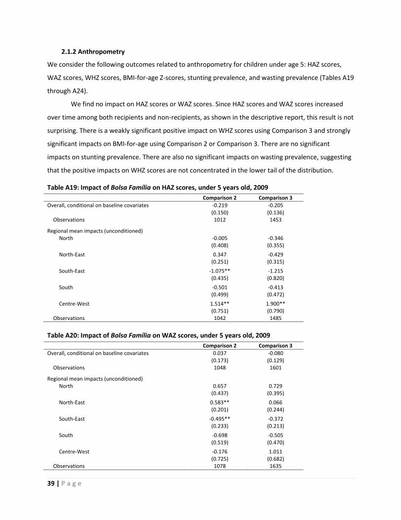
39 | P a g e
2.1.2 Anthropometry
We consider the following outcomes related to anthropometry for children under age 5: HAZ scores,
WAZ scores, WHZ scores, BMI-for-age Z-scores, stunting prevalence, and wasting prevalence (Tables A19
through A24).
We find no impact on HAZ scores or WAZ scores. Since HAZ scores and WAZ scores increased
over time among both recipients and non-recipients, as shown in the descriptive report, this result is not
surprising. There is a weakly significant positive impact on WHZ scores using Comparison 3 and strongly
significant impacts on BMI-for-age using Comparison 2 or Comparison 3. There are no significant
impacts on stunting prevalence. There are also no significant impacts on wasting prevalence, suggesting
that the positive impacts on WHZ scores are not concentrated in the lower tail of the distribution.
Table A19: Impact of Bolsa Família on HAZ scores, under 5 years old, 2009
Comparison 2 Comparison 3
Overall, conditional on baseline covariates -0.219 -0.205
(0.150) (0.136)
Observations 1012 1453
Regional mean impacts (unconditioned) North -0.005 -0.346
(0.408) (0.355)
North-East 0.347 -0.429
(0.251) (0.315)
South-East -1.075** -1.215
(0.435) (0.820)
South -0.501 -0.413
(0.499) (0.472)
Centre-West 1.514** 1.900**
(0.751) (0.790)
Observations 1042 1485
Table A20: Impact of Bolsa Família on WAZ scores, under 5 years old, 2009
Comparison 2 Comparison 3
Overall, conditional on baseline covariates 0.037 -0.080
(0.173) (0.129)
Observations 1048 1601
Regional mean impacts (unconditioned) North 0.657 0.729
(0.437) (0.395)
North-East 0.583** 0.066
(0.201) (0.244)
South-East -0.495** -0.372
(0.233) (0.213)
South -0.698 -0.505
(0.519) (0.470)
Centre-West -0.176 1.011
(0.725) (0.682)
Observations 1078 1635

40 | P a g e
Table A21: Impact of Bolsa Família on WHZ scores, under 5 years old, 2009
Comparison 2 Comparison 3
Overall, conditional on baseline covariates 0.132 0.287*
(0.214) (0.161)
Observations 961 1403
Regional mean impacts (unconditioned) North 0.743 0.713
(0.459) (0.406)
North-East 0.872** 0.559*
(0.232) (0.293)
South-East -0.053 0.102
(0.227) (0.213)
South -1.075 -0.616
(0.638) (0.543)
Centre-West 0.862 1.101
(0.625) (0.743)
Observations 987 1431
Table A22: Impact of Bolsa Família on BMI-for-Age Z-scores, under 5 years old, 2009
Comparison 2 Comparison 3
Overall, conditional on baseline covariates 0.342 0.298
(0.197)* (0.175)*
Observations 974 1500
Regional mean impacts (unconditioned) North 0.563 0.548
(0.431) (0.388)
North-East 0.755 0.568
(0.250) (0.311)
South-East 0.260 0.923
(0.334) (0.692)
South -0.048 0.316
(0.506) (0.535)
Centre-West 0.710 0.992
(0.617) (0.717)
Observations 1002 1533
Table A23: Impact of Bolsa Família on stunting prevalence, under 5 years old, 2009
Comparison 2 Comparison 3
Overall, conditional on baseline covariates 0.026 0.016
(0.036) (0.025)
Observations 1250 1906
Regional mean impacts (unconditioned) North 0.033 0.054
(0.110) (0.082)
North-East -0.064 0.014
(0.071) (0.035)
South-East 0.050 0.056**
(0.029) (0.022)
South 0.093 0.076
(0.145) (0.126)
Centre-West -0.407** -0.461**
(0.190) (0.229)
Observations 1290 1954
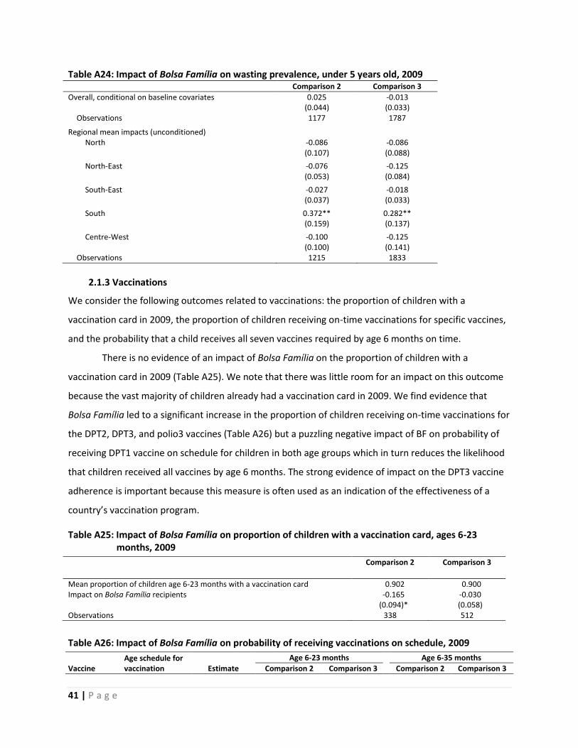
41 | P a g e
Table A24: Impact of Bolsa Família on wasting prevalence, under 5 years old, 2009
Comparison 2 Comparison 3
Overall, conditional on baseline covariates 0.025 -0.013
(0.044) (0.033)
Observations 1177 1787
Regional mean impacts (unconditioned) North -0.086 -0.086
(0.107) (0.088)
North-East -0.076 -0.125
(0.053) (0.084)
South-East -0.027 -0.018
(0.037) (0.033)
South 0.372** 0.282**
(0.159) (0.137)
Centre-West -0.100 -0.125
(0.100) (0.141)
Observations 1215 1833
2.1.3 Vaccinations
We consider the following outcomes related to vaccinations: the proportion of children with a
vaccination card in 2009, the proportion of children receiving on-time vaccinations for specific vaccines,
and the probability that a child receives all seven vaccines required by age 6 months on time.
There is no evidence of an impact of Bolsa Família on the proportion of children with a
vaccination card in 2009 (Table A25). We note that there was little room for an impact on this outcome
because the vast majority of children already had a vaccination card in 2009. We find evidence that
Bolsa Família led to a significant increase in the proportion of children receiving on-time vaccinations for
the DPT2, DPT3, and polio3 vaccines (Table A26) but a puzzling negative impact of BF on probability of
receiving DPT1 vaccine on schedule for children in both age groups which in turn reduces the likelihood
that children received all vaccines by age 6 months. The strong evidence of impact on the DPT3 vaccine
adherence is important because this measure is often used as an indication of the effectiveness of a
country’s vaccination program.
Table A25: Impact of Bolsa Família on proportion of children with a vaccination card, ages 6-23 months, 2009
Comparison 2 Comparison 3
Mean proportion of children age 6-23 months with a vaccination card 0.902 0.900 Impact on Bolsa Família recipients -0.165 -0.030
(0.094)* (0.058)
Observations 338 512
Table A26: Impact of Bolsa Família on probability of receiving vaccinations on schedule, 2009
Vaccine Age schedule for vaccination Estimate
Age 6-23 months Age 6-35 months
Comparison 2 Comparison 3 Comparison 2 Comparison 3

42 | P a g e
BCG At birth ATT 0.012 0.017 0.032 0.051 Standard error (0.050) (0.035) (0.047) (0.035) N 267 403 477 734
HBV1 At birth ATT -0.029 0.020 0.004 0.015 Standard error (0.056) (0.052) (0.058) (0.050) N 270 406 483 742
HBV2 2-4 months ATT -0.010 -0.002 -0.020 -0.030 Standard error (0.039) (0.030) (0.027) (0.022) N 273 407 483 739
DPT1 2 months ATT -0.148 -0.117 -0.107 -0.116 Standard error (0.076)* (0.061)* (0.060)* (0.045)** N 219 336 387 600
Polio1 2 months ATT -0.089 -0.010 -0.051 -0.052 Standard error (0.073) (0.057) (0.058) (0.043) N 273 408 488 744
DPT2 4 months ATT 0.258 0.155 0.298 0.239 Standard error (0.106)** (0.074)** (0.080)*** (0.060)*** N 204 318 365 575
Polio2 4 months ATT 0.116 0.069 0.141 0.132 Standard error (0.084) (0.076) (0.077)* (0.066)** N 273 407 485 737
HBV3 6 months ATT -0.011 0.032 0.020 0.057 Standard error (0.064) (0.055) (0.048) (0.040) N 261 391 468 715
DPT3 6 months ATT 0.348 0.260 0.325 0.253 Standard error (0.097)*** (0.087)*** (0.086)*** (0.066)*** N 197 301 352 547
Polio3 6 months ATT 0.148 0.116 0.170 0.128 Standard error (0.079)* (0.070)* (0.071)** (0.058)** N 255 377 463 702
SAR 12 months ATT 0.121 0.009 0.220 0.023 Standard error (0.099) (0.113) (0.096)** (0.074) N 99 143 189 287
Table A27: Impact of Bolsa Família on aggregate measures of timely vaccinations, 2009
Comparison 2 Comparison 3
Received the first seven vaccines by age 6 months -0.208 0.009
(0.107)* (0.071)
Observations 338 512
Number of vaccines received by age 6 months -1.632 -0.546
(0.616)*** (0.392)
Observations 338 512
Received no vaccines by age 6 months 0.188 0.080
(0.089)** (0.059)
Observations 323 489
Notes: The first seven recommended vaccines include BCG, HBV1, HBV2, DPT1, polio1, DPT2, and polio2.
2.1.4 Education
We consider the following outcomes related to education: the proportion of children currently
attending school, the proportion of children in school last year that progressed to the next grade level,
the proportion of children in school last year that are repeating the grade level, and the proportion of
children in school last year that dropped out (Tables A28 through A51).

43 | P a g e
In general, we find the following: disaggregated by sex, schooling impacts tend to be
concentrated among girls. Disaggregated by region, schooling impacts tend to be concentrated in the
North-East. Disaggregated by age, schooling impacts tend to be concentrated among 15-year-olds and
17-year-olds.
Specifically, in the North-East, among children age 6-17, there are significant increases in the
proportion currently attending, significant increases in the proportion progressing to the next grade
level, insignificant changes in the proportion repeating the previous grade level, and significant
decreases in the proportion dropping out.
There are significant increases in the proportion currently attending among 15-year-old girls and
17-year-old girls. There are highly significant decreases in the proportion dropping out among 17-year-
old girls and weakly significant increases in the proportion dropping out among 16-year-old girls. There
are (weakly) significant increases in the proportion progressing to the next grade level among 17-year-
old girls and (weakly) significant decreases in the proportion repeating a grade level among 16-year-old
girls. There appear to be no consistent impacts among males.
Table A28: Impact of Bolsa Família on proportion of children “currently attending school”, 2009
Comparison 2 Comparison 3
Overall, conditional on baseline covariates Children age 6-17 0.045 0.041
(0.026) * (0.025)
Observations 6514 10993
Regional mean impacts (unconditioned) Children age 6-17 North -0.032 -0.006
(0.051) (0.042)
North-East 0.161 0.199
(0.051) *** (0.058) ***
South-East -0.034 -0.009
(0.063) (0.052)
South -0.156 -0.111
(0.087) * (0.073)
Centre-West 0.040 0.020
(0.029) * (0.033)
Observations 6749 11361
Table A29: Impact of Bolsa Família on proportion of children in school last year that progressed to next grade level, 2009
Comparison 2 Comparison 3
Overall, conditional on baseline covariates Children age 6-17 0.037 0.069
(0.035) (0.033) **
Observations 4539 7703
Regional mean impacts (unconditioned)

44 | P a g e
Children age 6-17 North -0.058 -0.051
(0.079) (0.064)
North-East 0.121 0.117
(0.070) * (0.062) *
South-East -0.012 0.087
(0.063) (0.074)
South 0.132 0.223
(0.183) (0.153)
Centre-West -0.082 -0.074
(0.085) (0.072)
Observations 4704 7956
Table A30: Impact of Bolsa Família on proportion of children in school last year that are repeating grade level, 2009
Comparison 2 Comparison 3
Overall, conditional on baseline covariates Children age 6-17 -0.008 -0.050
(0.032) (0.030) *
Observations 4539 7703
Regional mean impacts (unconditioned)
Children age 6-17 North 0.059 0.060
(0.054) (0.045)
North-East 0.001 0.021
(0.052) (0.040)
South-East -0.017 -0.128
(0.046) (0.073) *
South -0.250 -0.283
(0.181) (0.153) *
Centre-West 0.076 0.060
(0.082) (0.067)
Observations 4704 7956

45 | P a g e
Table A31: Impact of Bolsa Família on proportion of children in school last year that dropped out, 2009
Comparison 2 Comparison 3
Overall, conditional on baseline covariates Children age 6-17 -0.029 -0.019
(0.022) (0.017)
Observations 4539 7703
Regional mean impacts (unconditioned)
Children age 6-17 North -0.000 -0.009
(0.069) (0.054)
North-East -0.122 -0.138
(0.048) ** (0.058) **
South-East 0.029 0.041
(0.050) (0.032)
South 0.118 0.060
(0.045) *** (0.022) ***
Centre-West 0.007 0.015
(0.021) (0.025)
Observations 4704 7956
Table A32: Impact of Bolsa Família on proportion of boys “currently attending school”, 2009
Comparison 2 Comparison 3
Overall, conditional on baseline covariates Males age 6-17 0.012 0.032
(0.035) (0.034)
Observations 3374 5633
Regional mean impacts (unconditioned)
Males age 6-17 North -0.032 -0.003
(0.063) (0.056)
North-East 0.114 0.229
(0.062) * (0.090) **
South-East -0.068 -0.011
(0.107) (0.087)
South -0.274 -0.062
(0.135) ** (0.111)
Centre-West 0.089 0.060
(0.047) * (0.054)
Observations 3491 5817

46 | P a g e
Table A33: Impact of Bolsa Família on proportion of girls “currently attending school”, 2009
Comparison 2 Comparison 3
Overall, conditional on baseline covariates Females age 6-17 0.082 0.038
(0.033) ** (0.034)
Observations 3133 5349
Regional mean impacts (unconditioned)
Females age 6-17 North -0.030 -0.008
(0.084) (0.061)
North-East 0.205 0.166
(0.074) *** (0.066) **
South-East -0.004 -0.013
(0.068) (0.046)
South -0.038 -0.189
(0.041) (0.086) **
Centre-West -0.004 -0.022
(0.039) (0.038)
Observations 3250 5532
Table A34: Impact of Bolsa Família on proportion of boys in school last year that progressed to next grade level, 2009
Comparison 2 Comparison 3
Overall, conditional on baseline covariates Males age 6-17 -0.033 0.006
(0.036) (0.039)
Observations 2312 3911
Regional mean impacts (unconditioned)
Males age 6-17 North -0.056 -0.035
(0.110) (0.096)
North-East 0.082 0.146
(0.102) (0.097)
South-East 0.011 0.111
(0.060) (0.098)
South -0.075 0.130
(0.250) (0.207)
Centre-West -0.088 -0.081
(0.136) (0.122)
Observations 2391 4030

47 | P a g e
Table A35: Impact of Bolsa Família on proportion of girls in school last year that progressed to next grade level, 2009
Comparison 2 Comparison 3
Overall, conditional on baseline covariates Females age 6-17 0.099 0.099
(0.048) ** (0.048) **
Observations 2222 3786
Regional mean impacts (unconditioned)
Females age 6-17 North -0.059 -0.068
(0.113) (0.081)
North-East 0.160 0.083
(0.086) * (0.074)
South-East -0.014 0.065
(0.105) (0.108)
South 0.338 0.348
(0.222) (0.203) *
Centre-West -0.030 -0.047
(0.061) (0.066)
Observations 2307 3919
Table A36: Impact of Bolsa Família on proportion of boys in school last year that are repeating grade level, 2009
Comparison 2 Comparison 3
Overall, conditional on baseline covariates Males age 6-17 0.057 -0.009
(0.033) * (0.038)
Observations 2312 3911
Regional mean impacts (unconditioned)
Males age 6-17 North 0.105 0.086
(0.093) (0.079)
North-East 0.033 0.057
(0.059) (0.039)
South-East -0.009 -0.135
(0.057) (0.099)
South -0.126 -0.201
(0.246) (0.204)
Centre-West 0.110 0.088
(0.134) (0.117)
Observations 2391 4030

48 | P a g e
Table A37: Impact of Bolsa Família on proportion of girls in school last year that are repeating grade level, 2009
Comparison 2 Comparison 3
Overall, conditional on baseline covariates Females age 6-17 -0.057 -0.084
(0.045) (0.042) **
Observations 2222 3786
Regional mean impacts (unconditioned)
Females age 6-17 North 0.005 0.032
(0.030) (0.031)
North-East -0.031 -0.019
(0.083) (0.072)
South-East -0.026 -0.111
(0.071) (0.103)
South -0.399 -0.400
(0.224) * (0.204) *
Centre-West -0.004 0.008
(0.042) (0.046)
Observations 2307 3919
Table A38: Impact of Bolsa Família on proportion of boys in school last year that dropped out, 2009
Comparison 2 Comparison 3
Overall, conditional on baseline covariates Males age 6-17 -0.024 0.003
(0.022) (0.016)
Observations 2312 3911
Regional mean impacts (unconditioned)
Males age 6-17 North -0.049 -0.051
(0.077) (0.071)
North-East -0.114 -0.203
(0.071) (0.099) **
South-East -0.002 0.024
(0.016) (0.013) *
South 0.202 0.071
(0.090) ** (0.037) *
Centre-West -0.022 -0.006
(0.027) (0.031)
Observations 2391 4030

49 | P a g e
Table A39: Impact of Bolsa Família on proportion of girls in school last year that dropped out, 2009
Comparison 2 Comparison 3
Overall, conditional on baseline covariates Females age 6-17 -0.042 -0.015
(0.032) (0.024)
Observations 2222 3786
Regional mean impacts (unconditioned) Females age 6-17 North 0.054 0.036
(0.116) (0.082)
North-East -0.129 -0.064
(0.064) ** (0.040)
South-East 0.040 0.046
(0.095) (0.063)
South 0.061 0.052
(0.034) * (0.023) **
Centre-West 0.034 0.039
(0.035) (0.041)
Observations 2307 3919
Table A40: Impact of Bolsa Família on proportion of children “currently attending school”, by age, 2009
Comparison 2 Comparison 3
Overall, conditional on baseline covariates Children age 6 0.027 0.147
(0.101) (0.079) * Obs 404 677 Children age 7 0.010 -0.015 (0.025) (0.036) Obs 420 745 Children age 13 0.073 0.081 (0.039) * (0.045) * Obs 595 1021 Children age 14 -0.081 -0.076 (0.035) ** (0.035) ** Obs 617 1020 Children age 15 0.187 0.158 (0.048) *** (0.057) *** Obs 651 1055 Children age 16 -0.049 -0.006 (0.054) (0.049) Obs 688 1068 Children age 17 0.070 0.004 (0.071) (0.069) Obs 601 945

50 | P a g e
Table A41: Impact of Bolsa Família on proportion of children in school last year that progressed to next grade level, by age, 2009
Comparison 2 Comparison 3
Overall, conditional on baseline covariates Children age 6 - -
- -
Children age 7 -0.223 -0.159 (0.084) *** (0.063) ** Obs 223 379 Children age 13 -0.015 0.085 (0.085) (0.072) Obs 472 816 Children age 14 -0.092 -0.104 (0.046) ** (0.042) ** Obs 469 777 Children age 15 0.182 0.172 (0.058) *** (0.057) *** Obs 441 726 Children age 16 0.072 0.029 (0.066) (0.079) Obs 474 729 Children age 17 0.037 0.047 (0.054) (0.054) Obs 392 608
Table A42: Impact of Bolsa Família on proportion of children in school last year that are repeating grade level, by age, 2009
Comparison 2 Comparison 3
Overall, conditional on baseline covariates Children age 6 - -
- - Children age 7 0.216 0.090 (0.080) *** (0.055)
Obs 223 379 Children age 13 0.042 -0.064 (0.088) (0.069)
Obs 472 816 Children age 14 0.004 0.031 (0.022) (0.025)
Obs 469 777 Children age 15 -0.058 -0.052 (0.055) (0.049)
Obs 441 726 Children age 16 -0.119 -0.093 (0.059) ** (0.062)
Obs 474 729 Children age 17 0.064 0.060 (0.047) (0.042)
Obs 392 608

51 | P a g e
Table A43: Impact of Bolsa Família on proportion of children in school last year that dropped out, by age, 2009
Comparison 2 Comparison 3
Overall, conditional on baseline covariates Children age 6 - -
- - Children age 7 0.008 0.068 (0.025) (0.029) **
Obs 223 379 Children age 13 -0.027 -0.020 (0.023) (0.024)
Obs 472 816 Children age 14 0.088 0.073 (0.039) ** (0.035) **
Obs 469 777 Children age 15 -0.124 -0.120 (0.040) *** (0.042) ***
Obs 441 726 Children age 16 0.048 0.064 (0.056) (0.048)
Obs 474 729 Children age 17 -0.102 -0.108 (0.038) *** (0.047) **
Obs 392 608
Table A44: Impact of Bolsa Família on proportion of boys “currently attending school”, by age, 2009
Comparison 2 Comparison 3
Overall, conditional on baseline covariates Males age 6 0.134 0.148
(0.061) ** (0.066) ** Obs 217 341
Males age 7 0.002 0.034 (0.041) (0.041)
Obs 220 378 Males age 13 0.055 0.091 (0.056) (0.061)
Obs 317 546 Males age 14 -0.042 -0.035 (0.037) (0.025)
Obs 311 531 Males age 15 0.222 0.244 (0.070) *** (0.074) ***
Obs 323 527 Males age 16 0.039 0.086 (0.056) (0.049) *
Obs 363 551 Males age 17 -0.012 -0.033 (0.078) (0.093)
Obs 305 492

52 | P a g e
Table A45: Impact of Bolsa Família on proportion of girls “currently attending school”, by age, 2009
Comparison 2 Comparison 3
Overall, conditional on baseline covariates Females age 6 0.244 0.254
(0.095) ** (0.076) *** Obs 186 335
Females age 7 -0.001 -0.031 (0.028) (0.028)
Obs 199 366 Females age 13 -0.011 -0.038 (0.021) (0.027)
Obs 277 473 Females age 14 -0.076 -0.084 (0.047) (0.046) *
Obs 306 488 Females age 15 0.178 0.143 (0.053) *** (0.064) **
Obs 328 528 Females age 16 -0.083 -0.078 (0.081) (0.067)
Obs 325 517 Females age 17 0.200 0.189 (0.073) *** (0.079) **
Obs 295 452
Table A46: Impact of Bolsa Família on proportion of boys in school last year that progressed to next grade level, by age, 2009
Comparison 2 Comparison 3
Overall, conditional on baseline covariates Males age 6 - -
- - Males age 7 -0.179 -0.114 (0.133) (0.093)
Obs 112 185 Males age 13 -0.152 -0.110 (0.078) * (0.054) **
Obs 249 435 Males age 14 -0.059 -0.082 (0.048) (0.044) *
Obs 233 403 Males age 15 0.125 0.237 (0.082) (0.091) ***
Obs 219 358 Males age 16 -0.009 0.074 (0.072) (0.069)
Obs 246 373 Males age 17 -0.013 -0.111 (0.083) (0.079)
Obs 197 310

53 | P a g e
Table A47: Impact of Bolsa Família on proportion of girls in school last year that progressed to next grade level, by age, 2009
Comparison 2 Comparison 3
Overall, conditional on baseline covariates Females age 6 - -
- - Females age 7 -0.186 -0.118 (0.132) (0.065) *
Obs 111 194 Females age 13 0.076 0.098 (0.113) (0.069)
Obs 222 380 Females age 14 -0.065 -0.101 (0.060) (0.055) *
Obs 236 374 Females age 15 0.209 0.173 (0.069) *** (0.059) ***
Obs 222 368 Females age 16 0.106 0.070 (0.085) (0.103)
Obs 228 356 Females age 17 -0.032 0.073 (0.076) (0.070)
Obs 194 297
Table A48: Impact of Bolsa Família on proportion of boys in school last year that are repeating grade level, by age, 2009
Comparison 2 Comparison 3
Overall, conditional on baseline covariates Males age 6 - -
- - Males age 7 0.206 0.112 (0.106) * (0.088)
Obs 112 185 Males age 13 0.167 0.104 (0.076) ** (0.047) **
Obs 249 435 Males age 14 0.011 0.031 (0.032) (0.036)
Obs 233 403 Males age 15 -0.027 -0.117 (0.087) (0.089)
Obs 219 358 Males age 16 0.029 -0.098 (0.059) (0.062)
Obs 246 373 Males age 17 0.065 0.130 (0.068) (0.056) **
Obs 197 310

54 | P a g e
Table A49: Impact of Bolsa Família on proportion of girls in school last year that are repeating grade level, by age, 2009
Comparison 2 Comparison 3
Overall, conditional on baseline covariates Females age 6 - -
- - Females age 7 0.175 0.084 (0.126) (0.057)
Obs 111 194 Females age 13 -0.071 -0.144 (0.113) (0.069) **
Obs 222 380 Females age 14 -0.018 0.019 (0.034) (0.034)
Obs 236 374 Females age 15 -0.096 -0.054 (0.059) (0.048)
Obs 222 368 Females age 16 -0.120 -0.104 (0.070) * (0.085)
Obs 228 356 Females age 17 0.110 0.034 (0.077) (0.073)
Obs 194 297
Table A50: Impact of Bolsa Família on proportion of boys in school last year that dropped out, by age, 2009
Comparison 2 Comparison 3
Overall, conditional on baseline covariates Males age 6 -
- Males age 7 -0.027 0.002 (0.064) (0.035)
Obs 112 185 Males age 13 -0.015 0.006 (0.038) (0.037)
Obs 249 435 Males age 14 0.048 0.050 (0.038) (0.024) **
Obs 233 403 Males age 15 -0.098 -0.120 (0.047) ** (0.050) **
Obs 219 358 Males age 16 -0.021 0.023 (0.045) (0.043)
Obs 246 373 Males age 17 -0.052 -0.019 (0.053) (0.062)
Obs 197 310
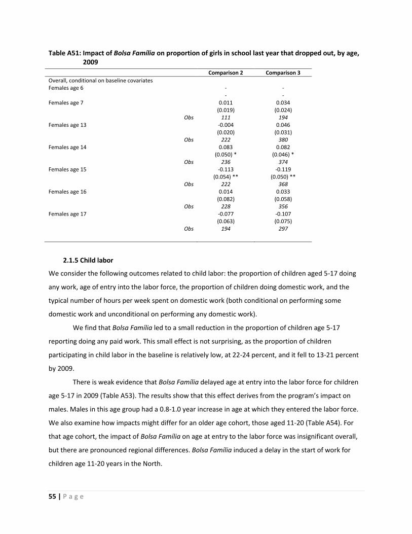
55 | P a g e
Table A51: Impact of Bolsa Família on proportion of girls in school last year that dropped out, by age, 2009
Comparison 2 Comparison 3
Overall, conditional on baseline covariates Females age 6 - -
- - Females age 7 0.011 0.034 (0.019) (0.024)
Obs 111 194 Females age 13 -0.004 0.046 (0.020) (0.031)
Obs 222 380 Females age 14 0.083 0.082 (0.050) * (0.046) *
Obs 236 374 Females age 15 -0.113 -0.119 (0.054) ** (0.050) **
Obs 222 368 Females age 16 0.014 0.033 (0.082) (0.058)
Obs 228 356 Females age 17 -0.077 -0.107 (0.063) (0.075)
Obs 194 297
2.1.5 Child labor
We consider the following outcomes related to child labor: the proportion of children aged 5-17 doing
any work, age of entry into the labor force, the proportion of children doing domestic work, and the
typical number of hours per week spent on domestic work (both conditional on performing some
domestic work and unconditional on performing any domestic work).
We find that Bolsa Família led to a small reduction in the proportion of children age 5-17
reporting doing any paid work. This small effect is not surprising, as the proportion of children
participating in child labor in the baseline is relatively low, at 22-24 percent, and it fell to 13-21 percent
by 2009.
There is weak evidence that Bolsa Família delayed age at entry into the labor force for children
age 5-17 in 2009 (Table A53). The results show that this effect derives from the program’s impact on
males. Males in this age group had a 0.8-1.0 year increase in age at which they entered the labor force.
We also examine how impacts might differ for an older age cohort, those aged 11-20 (Table A54). For
that age cohort, the impact of Bolsa Família on age at entry to the labor force was insignificant overall,
but there are pronounced regional differences. Bolsa Família induced a delay in the start of work for
children age 11-20 years in the North.
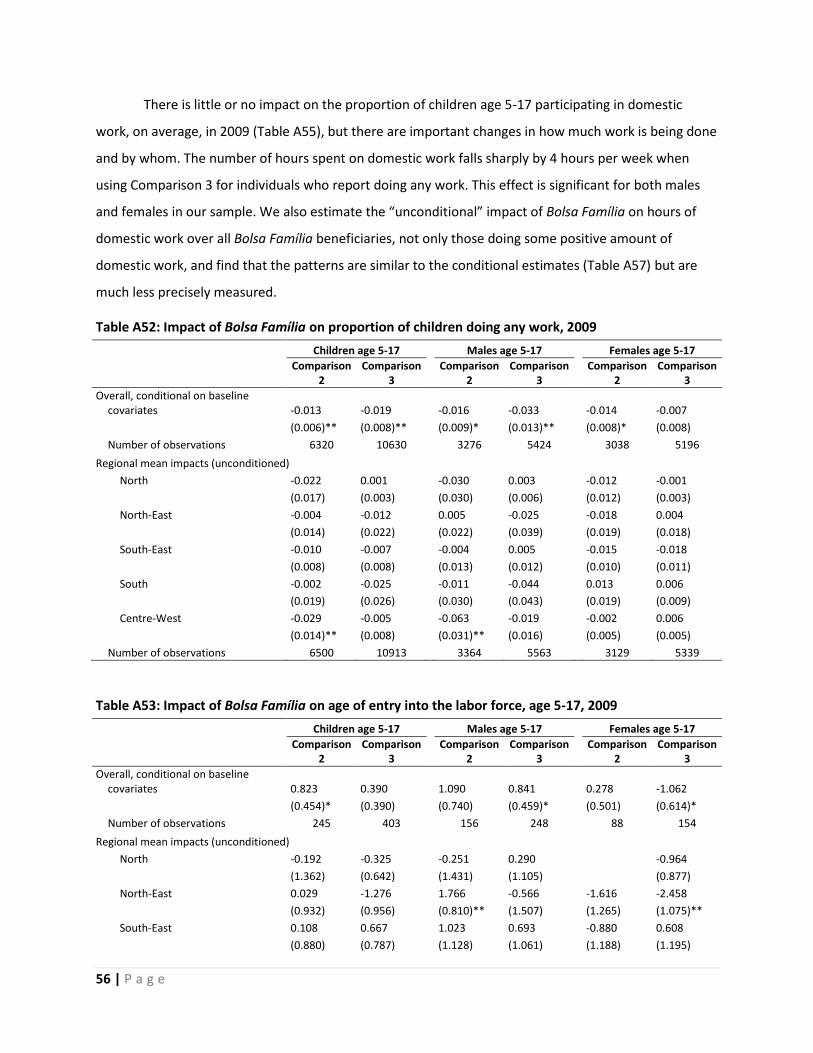
56 | P a g e
There is little or no impact on the proportion of children age 5-17 participating in domestic
work, on average, in 2009 (Table A55), but there are important changes in how much work is being done
and by whom. The number of hours spent on domestic work falls sharply by 4 hours per week when
using Comparison 3 for individuals who report doing any work. This effect is significant for both males
and females in our sample. We also estimate the “unconditional” impact of Bolsa Família on hours of
domestic work over all Bolsa Família beneficiaries, not only those doing some positive amount of
domestic work, and find that the patterns are similar to the conditional estimates (Table A57) but are
much less precisely measured.
Table A52: Impact of Bolsa Família on proportion of children doing any work, 2009
Children age 5-17
Males age 5-17
Females age 5-17
Comparison 2
Comparison 3
Comparison 2
Comparison 3
Comparison 2
Comparison 3
Overall, conditional on baseline covariates -0.013 -0.019
-0.016 -0.033
-0.014 -0.007
(0.006)** (0.008)**
(0.009)* (0.013)**
(0.008)* (0.008)
Number of observations 6320 10630
3276 5424
3038 5196
Regional mean impacts (unconditioned) North -0.022 0.001
-0.030 0.003
-0.012 -0.001
(0.017) (0.003)
(0.030) (0.006)
(0.012) (0.003)
North-East -0.004 -0.012 0.005 -0.025
-0.018 0.004
(0.014) (0.022)
(0.022) (0.039)
(0.019) (0.018)
South-East -0.010 -0.007 -0.004 0.005
-0.015 -0.018
(0.008) (0.008)
(0.013) (0.012)
(0.010) (0.011)
South -0.002 -0.025 -0.011 -0.044
0.013 0.006
(0.019) (0.026)
(0.030) (0.043)
(0.019) (0.009)
Centre-West -0.029 -0.005 -0.063 -0.019
-0.002 0.006
(0.014)** (0.008)
(0.031)** (0.016)
(0.005) (0.005)
Number of observations 6500 10913
3364 5563
3129 5339
Table A53: Impact of Bolsa Família on age of entry into the labor force, age 5-17, 2009
Children age 5-17
Males age 5-17
Females age 5-17
Comparison 2
Comparison 3
Comparison 2
Comparison 3
Comparison 2
Comparison 3
Overall, conditional on baseline covariates 0.823 0.390
1.090 0.841
0.278 -1.062
(0.454)* (0.390)
(0.740) (0.459)*
(0.501) (0.614)*
Number of observations 245 403
156 248
88 154
Regional mean impacts (unconditioned) North -0.192 -0.325
-0.251 0.290
-0.964
(1.362) (0.642)
(1.431) (1.105)
(0.877)
North-East 0.029 -1.276 1.766 -0.566
-1.616 -2.458
(0.932) (0.956)
(0.810)** (1.507)
(1.265) (1.075)**
South-East 0.108 0.667 1.023 0.693
-0.880 0.608
(0.880) (0.787)
(1.128) (1.061)
(1.188) (1.195)
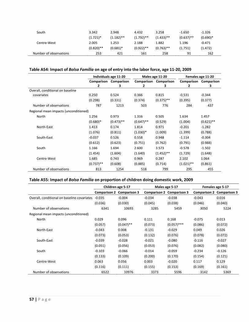
57 | P a g e
South 3.342 2.948 4.432 3.258
-1.650 -1.326
(1.721)* (1.182)**
(1.792)** (1.433)**
(0.637)** (0.690)*
Centre-West 2.005 1.253 2.188 1.882
1.196 -0.471
(0.820)** (0.681)*
(0.922)** (0.763)**
(1.751) (1.472)
Number of observations 253 421
161 258
91 162
Table A54: Impact of Bolsa Família on age of entry into the labor force, age 11-20, 2009
Individuals age 11-20
Males age 11-20
Females age 11-20
Comparison 2
Comparison 3
Comparison 2
Comparison 3
Comparison 2
Comparison 3
Overall, conditional on baseline covariates 0.250 0.524
0.366 0.815
-0.531 -0.344
(0.298) (0.331)
(0.374) (0.375)**
(0.395) (0.377)
Number of observations 787 1213
503 776
284 437
Regional mean impacts (unconditioned) North 1.256 0.973
1.316 0.505
1.634 1.457
(0.680)* (0.473)**
(0.647)** (0.529)
(1.004) (0.621)**
North-East 1.413 0.174 1.814 0.971
-0.201 -1.282
(1.076) (0.811)
(1.030)* (1.009)
(1.399) (0.788)
South-East -0.037 0.526 0.558 0.948
-1.114 -0.304
(0.612) (0.623)
(0.751) (0.762)
(0.791) (0.988)
South 1.166 1.694 2.600 3.573
-0.578 -1.502
(1.454) (1.604)
(1.640) (1.452)**
(1.729) (1.648)
Centre-West 1.685 0.743 0.969 0.287
2.102 1.064
(0.737)** (0.608)
(0.885) (0.714)
(1.021)** (0.861)
Number of observations 813 1254
518 799
295 455
Table A55: Impact of Bolsa Família on proportion of children doing domestic work, 2009
Children age 5-17
Males age 5-17
Females age 5-17
Comparison 2 Comparison 3
Comparison 2 Comparison 3
Comparison 2 Comparison 3
Overall, conditional on baseline covariates -0.035 -0.004 -0.034 -0.038
-0.043 0.016
(0.036) (0.030)
(0.045) (0.038)
(0.046) (0.040)
Number of observations 6341 10693
3285 5459
3050 5224
Regional mean impacts (unconditioned) North 0.029 0.096
0.111 0.168
-0.075 0.013
(0.057) (0.047)**
(0.073) (0.057)***
(0.086) (0.072)
North-East -0.043 0.008 -0.131 -0.029
0.049 0.026
(0.073) (0.053)
(0.132) (0.076)
(0.078) (0.072)
South-East -0.039 -0.028 -0.021 -0.080
-0.116 -0.027
(0.051) (0.056)
(0.053) (0.076)
(0.082) (0.080)
South -0.103 -0.066 -0.014 -0.059
-0.234 -0.126
(0.133) (0.109)
(0.200) (0.170)
(0.154) (0.121)
Centre-West 0.063 0.056 0.003 -0.020
0.117 0.129
(0.116) (0.111)
(0.155) (0.153)
(0.169) (0.161)
Number of observations 6522 10976
3373 5596
3142 5369

58 | P a g e
Table A56: Impact of Bolsa Família on typical number of hours per week spent on domestic work, conditional on performing some domestic work, 2009
Children age 5-17
Males age 5-17
Females age 5-17
Comparison 2
Comparison 3
Comparison 2
Comparison 3
Comparison 2
Comparison 3
Overall, conditional on baseline covariates -1.688 -4.486
-0.293 -5.163
-1.803 -2.955
(1.313) (1.329)***
(2.099) (1.776)***
(1.609) (1.712)*
Number of observations 2469 4151
911 1490
1555 2657
Regional mean impacts (unconditioned) North -0.365 -3.173
-3.446 -9.420
1.961 0.626
(2.060) (2.946)
(3.188) (5.627)*
(2.707) (3.310)
North-East 3.031 -0.208 4.462 1.514
0.379 -1.900
(3.475) (2.277)
(2.423)* (2.486)
(3.010) (2.273)
South-East -5.053 -12.020 -11.736 -25.445
-0.935 -0.220
(3.325) (6.787)*
(6.849)* (10.337)**
(2.434) (2.337)
South -8.514 -6.993 -6.195 -7.415
-11.845 -6.020
(3.551)** (3.761)*
(5.347) (4.889)
(4.432)*** (5.481)
Centre-West -3.385 -2.300 -3.994 -4.231
-2.795 -0.632
(1.736)* (1.659)
(2.984) (2.803)
(1.767) (1.782)
Number of observations 2530 4248
928 1517
1599 2727
Table A57: Impact of Bolsa Família on typical number of hours per week spent on domestic work,
unconditional on performing some domestic work, 2009
Children age 5-17
Males age 5-17
Females age 5-17
Comparison 2
Comparison 3
Comparison 2
Comparison 3
Comparison 2
Comparison 3
Overall, conditional on baseline covariates -0.461 -0.673
-0.461 -1.187
-0.362 0.173
(0.706) (0.772)
(0.814) (0.856)
(1.102) (1.095)
Number of observations 7021 11711
3624 5976
3391 5725
Regional mean impacts (unconditioned) North 0.158 0.484
0.872 0.498
-0.746 0.368
(0.984) (0.988)
(1.355) (1.353)
(1.447) (1.451)
North-East 1.640 0.950 0.739 0.454
2.870 1.097
(0.889)* (0.793)
(0.420)* (0.479)
(1.640)* (1.505)
South-East -1.122 -3.558 -1.719 -6.828
-1.009 0.105
(1.128) (2.775)
(1.611) (4.463)
(1.277) (1.312)
South -6.853 -3.923 -4.124 -4.032
-10.094 -4.073
(4.334) (3.709)
(6.128) (5.112)
(5.756)* (5.247)
Centre-West -0.017 1.471 -0.889 0.545
0.791 2.386
(0.943) (0.757)*
(1.334) (1.119)
(1.299) (1.018)**
Number of observations 7228 12026
3722 6128
3494 5882

59 | P a g e
2.2 Women’s welfare
2.2.1 Impact on prenatal care
We consider the following outcomes related to prenatal care, both among a sample of women pregnant
during the 2009 AIBF survey and among a sample of women pregnant between the 2005 and 2009
survey: the number of prenatal care visits, the proportion of women having no prenatal care visits, the
proportion of women receiving adequate prenatal care, and the proportion of women receiving prenatal
care from a doctor rather than a nurse or informal care provider.
We find qualified evidence that BF increased use of prenatal care. BF recipients who were
pregnant at the time of the 2009 survey had 1.7 more prenatal care visits than pregnant women who
were non-recipients (Table A58). We find this result across models using both comparison groups;
however, the result is qualified because of the relatively small samples of women pregnant at the time
of the 2009 interview. With such a small sample of women who were pregnant at the time of the
interview, estimates of impacts at the regional level are not very precise, but the relative magnitudes of
the estimated regional effects is still informative. Results show that the impact of Bolsa Família on the
number of prenatal care visits was largest in the North and was also quite large in the North-East and
South-East.

60 | P a g e
Table A58: Impact of Bolsa Família on the number of prenatal care visits, for women pregnant during the 2009 AIBF survey
Comparison 2 Comparison 3
Overall, conditional on baseline covariates 1.701 1.602
(0.913)* (0.800)**
Observations 75 121
Regional mean impacts (unconditioned)
North 5.042 4.864
(1.261)*** (1.142)***
North-East 6.155 5.842
(1.146)*** (0.860)***
South-East 3.071 2.648
(1.235)** (1.420)*
South -2.500 -1.149
(0.755)*** (0.981)
Centre-West -1.834 -2.146
(0.929)* (0.575)***
Observations 78 125
There is no evidence that Bolsa Família reduced the proportion of pregnant women in the 2009
survey who had no prenatal care visits across the full sample (Table A59). At the regional level, Bolsa
Família appears to have reduced the proportion of women having no prenatal care visits, but the size of
this effect cannot be precisely estimated. We also cannot conclude that Bolsa Família had an impact on
the proportion of women who obtained timely and adequate prenatal care for their stage of pregnancy
among women who were pregnant in the 2009 survey (Table A60). Estimated regional effects show
positive impacts of Bolsa Família on the proportion of women who obtained adequate prenatal care in
the North-East and negative impacts in the North, but samples are too small for these estimates to be
considered reliable. There is also no evidence that participation in Bolsa Família decreased the
probability that a woman's prenatal care visits were in consultation with a doctor, rather than a nurse or
informal care provider (Table A61).
For pregnancies reported between the 2005 and 2009 survey rounds, there is no evidence for
the full sample that Bolsa Família reduced the proportion of women who had no prenatal care visits
(Table A62), increased the proportion of women who had at least six prenatal care visits (Table A63), or
increased the probability that a woman's prenatal care visits were attended by a doctor (Table A64), if
anything there is an imprecisely measured negative effect.
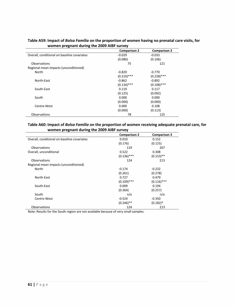
61 | P a g e
Table A59: Impact of Bolsa Família on the proportion of women having no prenatal care visits, for women pregnant during the 2009 AIBF survey
Comparison 2 Comparison 3
Overall, conditional on baseline covariates -0.029 -0.033
(0.080) (0.106)
Observations 75 121 Regional mean impacts (unconditioned)
North -0.820 -0.770
(0.210)*** (0.228)***
North-East -0.862 -0.892
(0.134)*** (0.108)***
South-East 0.119 0.117
(0.125) (0.092)
South 0.000 0.000
(0.000) (0.000)
Centre-West 0.000 0.108
(0.000) (0.113)
Observations 78 125
Table A60: Impact of Bolsa Família on the proportion of women receiving adequate prenatal care, for
women pregnant during the 2009 AIBF survey
Comparison 2 Comparison 3
Overall, conditional on baseline covariates 0.010 0.152
(0.176) (0.125)
Observations 119 207 Overall, unconditional 0.522 0.308
(0.136)*** (0.153)**
Observations 124 213 Regional mean impacts (unconditioned)
North -0.174 -0.232
(0.261) (0.278)
North-East 0.727 0.479
(0.109)*** (0.116)***
South-East 0.009 0.194
(0.364) (0.257)
South n/a n/a Centre-West -0.524 -0.350
(0.246)** (0.182)*
Observations 124 213
Note: Results for the South region are not available because of very small samples.

62 | P a g e
Table A61: Impact of Bolsa Família on the proportion of women receiving prenatal care from a doctor rather than a nurse or informal care provider, for women pregnant during the 2009 AIBF survey
Comparison 2 Comparison 3
Overall, conditional on baseline covariates -0.008 0.079
(0.137) (0.122)
Observations 119 207 Regional mean impacts (unconditioned)
North 0.550 0.393
(0.238)** (0.218)*
North-East 0.502 0.324
(0.173)*** (0.120)***
South-East -0.051 0.115
(0.360) (0.260)
South -0.391 -0.500
(0.310) (0.298)*
Centre-West -0.259 -0.553
(0.333) (0.227)**
Observations 124 213
Table A62: Impact of Bolsa Família on the proportion of women having no prenatal care visits, for
women pregnant between the 2005 and 2009 AIBF surveys
Comparison 2 Comparison 3
Overall, conditional on baseline covariates 0.001 0.019
(0.020) (0.016)
Observations 675 1015 Regional mean impacts (unconditioned)
North -0.047 -0.031
(0.051) (0.053)
North-East 0.024 0.035
(0.025) (0.021)*
South-East -0.005 0.076
(0.016) (0.058)
South -0.003 0.004
(0.005) (0.018)
Centre-West 0.069 0.115
(0.079) (0.075)
Observations 695 1038

63 | P a g e
Table A63: Impact of Bolsa Família on the proportion of women receiving adequate prenatal care, for women pregnant between the 2005 and 2009 AIBF surveys
Comparison 2 Comparison 3
Overall, conditional on baseline covariates 0.064 -0.026
(0.054) (0.049)
Observations 675 1015 Regional mean impacts (unconditioned)
North -0.069 -0.168
(0.155) (0.122)
North-East 0.069 -0.027
(0.118) (0.092)
South-East 0.170 0.227
(0.091)* (0.165)
South -0.090 -0.148
(0.088) (0.087)*
Centre-West -0.177 -0.179
(0.142) (0.102)*
Observations 695 1038
Table A64: Impact of Bolsa Família on the proportion of women receiving prenatal care from a doctor
rather than a nurse or informal care provider, for women pregnant between the 2005 and 2009 AIBF surveys
Comparison 2 Comparison 3
Overall, conditional on baseline covariates -0.106 -0.122
(0.063)* (0.052)**
Observations 789 1189 Regional mean impacts (unconditioned)
North 0.244 0.171
(0.149) (0.144)
North-East -0.210 -0.214
(0.114)* (0.115)*
South-East 0.027 -0.080
(0.063) (0.070)
South 0.043 0.094
(0.160) (0.221)
Centre-West -0.406 -0.455
(0.191)** (0.139)***
Observations 812 1216
2.2.2 Decisionmaking within the household
We consider the following outcomes related to women’s decisionmaking power: the proportion of
women who report being the sole decisionmaker on food purchases, the proportion of women who
report being the sole decisionmaker on clothes for herself, the proportion of women who report being
the sole decisionmaker on clothes for her children, the proportion of women who report being the sole
decisionmaker on school expenditures, the proportion of women who report being the sole
decisionmaker on medicine for children, the proportion of women who report being the sole
decisionmaker on durable goods, the proportion of women who report being the sole decisionmaker on

64 | P a g e
labor, and the proportion of women who report being the sole decisionmaker on contraception (Tables
A65 through A72).
We find strong positive impacts in the full sample on women’s decisionmaking power related to
medicine for children, durable goods, and contraception. Although several of these results are only
weakly significant using propensity score weighting, we confirm that when we re-estimate impacts for
these outcomes using the more computationally-intensive but lower-variance method of covariate
matching, the impacts are significant at the 5 percent level.
Table A65: Impact of Bolsa Família on women’s decisionmaking power, food purchases, 2009
Comparison 2 Comparison 3
Overall, conditional on baseline covariates 0.002 0.011
(0.046) (0.038)
Observations 2440 3663
Regional mean impacts (unconditioned) North 0.139 0.067
(0.088) (0.074)
North-East -0.103 -0.117
(0.085) (0.074)
South-East 0.105 0.101
(0.112) (0.088)
South 0.257* 0.395**
(0.164) (0.141)
Centre-West -0.094 -0.205
(0.152) (0.151)
Observations 2497 3754
Table A66: Impact of Bolsa Família on women’s decisionmaking power, clothes for self, 2009
Comparison 2 Comparison 3
Overall, conditional on baseline covariates 0.031 0.043
0.046 (0.039)
Observations 2424 3636
Regional mean impacts (unconditioned) North 0.176* 0.132
(0.104) (0.085)
North-East -0.109 -0.116*
0.077 (0.060)
South-East 0.112 0.071
(0.100) (0.091)
South 0.239 0.431**
(0.163) (0.131)
Centre-West 0.101 0.100
(0.165) (0.149)
Observations 2480 3725
Table A67: Impact of Bolsa Família on women’s decisionmaking power, clothes for children, 2009
Comparison 2 Comparison 3
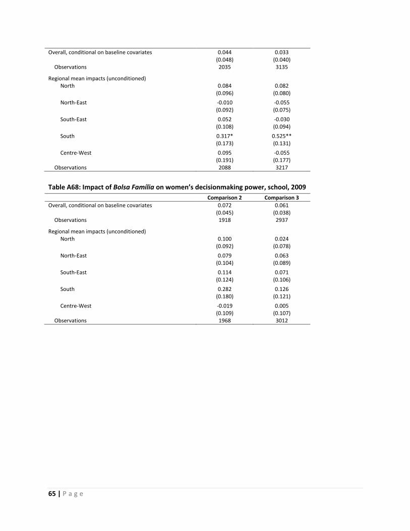
65 | P a g e
Overall, conditional on baseline covariates 0.044 0.033
(0.048) (0.040)
Observations 2035 3135
Regional mean impacts (unconditioned) North 0.084 0.082
(0.096) (0.080)
North-East -0.010 -0.055
(0.092) (0.075)
South-East 0.052 -0.030
(0.108) (0.094)
South 0.317* 0.525**
(0.173) (0.131)
Centre-West 0.095 -0.055
(0.191) (0.177)
Observations 2088 3217
Table A68: Impact of Bolsa Família on women’s decisionmaking power, school, 2009
Comparison 2 Comparison 3
Overall, conditional on baseline covariates 0.072 0.061
(0.045) (0.038)
Observations 1918 2937
Regional mean impacts (unconditioned) North 0.100 0.024
(0.092) (0.078)
North-East 0.079 0.063
(0.104) (0.089)
South-East 0.114 0.071
(0.124) (0.106)
South 0.282 0.126
(0.180) (0.121)
Centre-West -0.019 0.005
(0.109) (0.107)
Observations 1968 3012
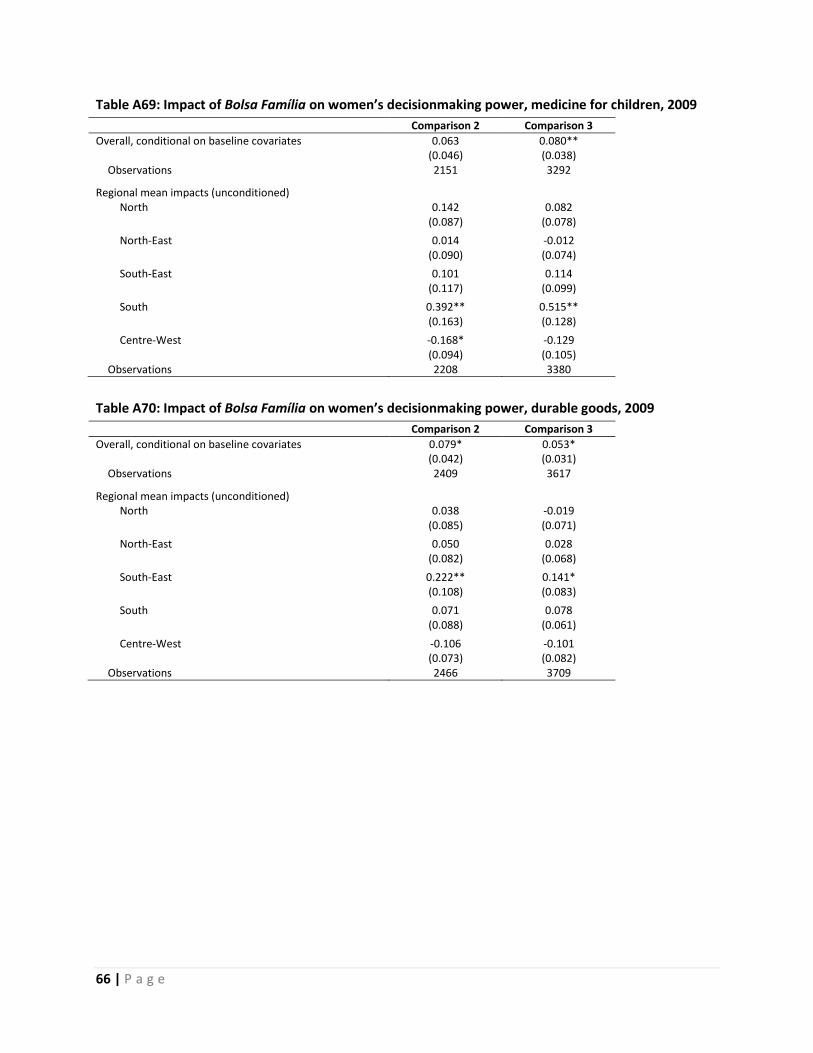
66 | P a g e
Table A69: Impact of Bolsa Família on women’s decisionmaking power, medicine for children, 2009
Comparison 2 Comparison 3
Overall, conditional on baseline covariates 0.063 0.080**
(0.046) (0.038)
Observations 2151 3292
Regional mean impacts (unconditioned) North 0.142 0.082
(0.087) (0.078)
North-East 0.014 -0.012
(0.090) (0.074)
South-East 0.101 0.114
(0.117) (0.099)
South 0.392** 0.515**
(0.163) (0.128)
Centre-West -0.168* -0.129
(0.094) (0.105)
Observations 2208 3380
Table A70: Impact of Bolsa Família on women’s decisionmaking power, durable goods, 2009
Comparison 2 Comparison 3
Overall, conditional on baseline covariates 0.079* 0.053*
(0.042) (0.031)
Observations 2409 3617
Regional mean impacts (unconditioned) North 0.038 -0.019
(0.085) (0.071)
North-East 0.050 0.028
(0.082) (0.068)
South-East 0.222** 0.141*
(0.108) (0.083)
South 0.071 0.078
(0.088) (0.061)
Centre-West -0.106 -0.101
(0.073) (0.082)
Observations 2466 3709

67 | P a g e
Table A71: Impact of Bolsa Família on women’s decisionmaking power, labor, 2009
Comparison 2 Comparison 3
Overall, conditional on baseline covariates 0.035 0.012
(0.045) (0.038)
Observations 2444 3650
Regional mean impacts (unconditioned) North 0.037 0.076
(0.096) (0.076)
North-East 0.038 -0.002
(0.081) (0.071)
South-East 0.009 -0.012
(0.104) (0.092)
South 0.331** 0.204*
(0.151) (0.107)
Centre-West -0.233 -0.291**
(0.167) (0.128)
Observations 2501 3741
Table A72: Impact of Bolsa Família on women’s decisionmaking power, contraception, 2009
Comparison 2 Comparison 3
Overall, conditional on baseline covariates 0.010** 0.098**
(0.045) (0.036)
Observations 2334 3509
Regional mean impacts (unconditioned) North 0.109 0.085
(0.083) (0.066)
North-East 0.097 0.065
(0.086) (0.074)
South-East 0.134 0.071
(0.111) (0.010)
South 0.271* 0.265**
(0.162) (0.123)
Centre-West 0.102 0.091
(0.148) (0.118)
Observations 2391 3596
2.3 Household behavior and welfare
2.3.1 Labor supply
We consider the following outcomes related to labor supply decisions: proportion of all individuals aged
18-55 that are currently working, proportion of individuals aged 18-55 in the labor force that are
currently working, and proportion of all individuals aged 18-55 not working that have sought work in the
past 30 days (Tables A73 through A75). Here, we define the “labor force” as all individuals aged 18-55
who either are currently working or are currently not working but have sought work in the past 30 days.
In general, there are very few significant impacts on these outcomes, either in the aggregate or
by sex (Tables A76 through A81). Aggregating over males and females, there appear to be no significant

68 | P a g e
impacts on the proportion of all individuals aged 18-55 that is currently working, on the proportion of
individuals aged 18-55 in the labor force that is currently working, and the proportion of individuals aged
18-55 not currently working that is seeking work. This tends to be the case disaggregated by region, as
well. Only in the North, there appears to be a significant or weakly significant decrease in the
proportion of individuals currently not working that have sought work in the past 30 days, by about -
0.08 to-0.11 (depending on the use of Comparison 2 or 3).
Among males only, there tend to be no significant impacts on these outcomes. Only according
to Comparison 2, there is a significant increase in the proportion of males currently working by about
0.06, as well as a significant increase in the proportion of the labor force currently working by about
0.06. In Comparison 3, these impacts are not significant. Among females only, there tend to be no
significant impacts on proportion currently working or proportion of the labor force currently working.
Only in the North-East, there appears to be a significant decrease in the proportion of females in the
labor force currently working by about -0.09 to -0.13 (depending on the use of Comparison 2 or 3).
There appears to be a weakly significant increase in the proportion of females that have sought work
among those not currently working, by about 0.05 to 0.07, which appears driven by the North-East,
where the increase is significant and roughly 0.09 to 0.11 (depending on the use of Comparison 2 or 3).
We also consider outcomes related to the contribution to household labor supply from different
household members and the allocation of household labor supply to different sectors of the labor
market: average total household weekly work hours among individuals aged 18-69, average formal
household weekly work hours among individuals aged 18-69, average informal household weekly work
hours among individuals aged 18-69, average total household weekly work hours among males aged 18-
69, average total household weekly work hours among females aged 18-69, average formal household
weekly work hours among males aged 18-69, average informal household weekly work hours among
males aged 18-69, average formal household weekly work hours among females aged 18-69, average
informal household weekly work hours among females aged 18-69, the proportion of total household
weekly work hours among individuals aged 18-69 devoted to formal sector, and the proportion of total
household weekly work hours among individuals aged 18-69 worked by females (Tables A82 through
A91). Here, we define a job as being in the formal sector if the household member either has a “card”
for that job or contributes to social security through that job.
Overall, there appears to be an insignificant impact on average total household weekly work
hours among individuals aged 18-69 per individual aged 18-69. This is the case for both males and
females. This is also the case when disaggregated by region, overall or by sex. However, there is a highly
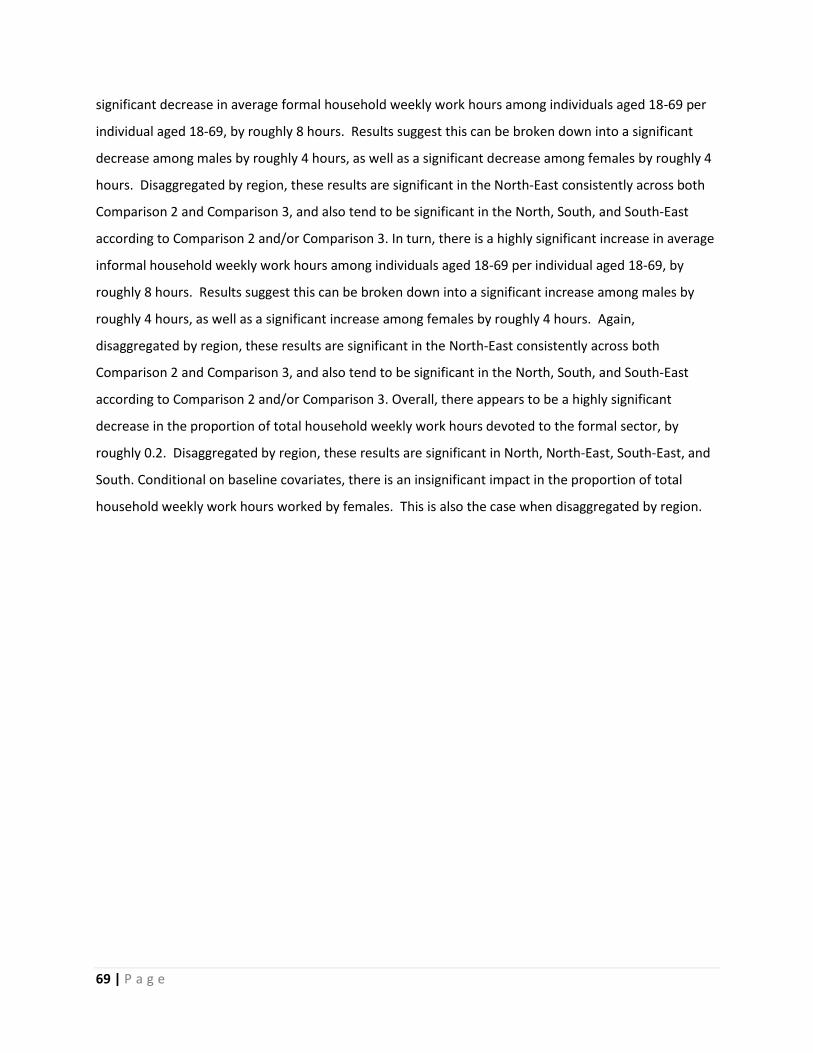
69 | P a g e
significant decrease in average formal household weekly work hours among individuals aged 18-69 per
individual aged 18-69, by roughly 8 hours. Results suggest this can be broken down into a significant
decrease among males by roughly 4 hours, as well as a significant decrease among females by roughly 4
hours. Disaggregated by region, these results are significant in the North-East consistently across both
Comparison 2 and Comparison 3, and also tend to be significant in the North, South, and South-East
according to Comparison 2 and/or Comparison 3. In turn, there is a highly significant increase in average
informal household weekly work hours among individuals aged 18-69 per individual aged 18-69, by
roughly 8 hours. Results suggest this can be broken down into a significant increase among males by
roughly 4 hours, as well as a significant increase among females by roughly 4 hours. Again,
disaggregated by region, these results are significant in the North-East consistently across both
Comparison 2 and Comparison 3, and also tend to be significant in the North, South, and South-East
according to Comparison 2 and/or Comparison 3. Overall, there appears to be a highly significant
decrease in the proportion of total household weekly work hours devoted to the formal sector, by
roughly 0.2. Disaggregated by region, these results are significant in North, North-East, South-East, and
South. Conditional on baseline covariates, there is an insignificant impact in the proportion of total
household weekly work hours worked by females. This is also the case when disaggregated by region.

70 | P a g e
Table A73: Impact of Bolsa Família on proportion of all individuals ages 18-55 that are currently working, 2009
Comparison 2 Comparison 3
Overall, conditional on baseline covariates 0.009 0.001
(0.027) (0.023)
Observations 10426 15518
Regional mean impacts (unconditioned) North -0.072 -0.034
(0.049) (0.042)
North-East 0.020 0.014
(0.057) (0.042)
South-East 0.004 0.015
(0.055) (0.045)
South 0.039 -0.016
(0.118) (0.093)
Centre-West 0.099 0.051
(0.089) (0.083)
Observations 10802 16045
Table A74: Impact of Bolsa Família on proportion of individuals aged 18-55 in the labor force that are currently working, 2009
Comparison 2 Comparison 3
Overall, conditional on baseline covariates 0.022 0.009
(0.031) (0.021)
Observations 6452 9505
Regional mean impacts (unconditioned) North 0.054 0.054
(0.047) (0.045)
North-East 0.047 0.008
(0.089) (0.050)
South-East -0.001 0.013
(0.047) (0.035)
South 0.001 -0.012
(0.115) (0.071)
Centre-West 0.043 -0.017
(0.060) (0.043)
Observations 6672 9819

71 | P a g e
Table A75: Impact of Bolsa Família on proportion of all individuals aged 18-55 not working that have sought work in the past 30 days, 2009
Comparison 2 Comparison 3
Overall, conditional on baseline covariates 0.006 0.007
(0.043) (0.032)
Observations 4643 7022
Regional mean impacts (unconditioned) North -0.111 -0.084
(0.056) ** (0.050) *
North-East -0.044 0.007
(0.111) (0.069)
South-East 0.011 -0.006
(0.070) (0.051)
South -0.033 -0.019
(0.136) (0.109)
Centre-West -0.006 0.065
(0.096) (0.067)
Observations 4831 7271
Table A76: Impact of Bolsa Família on proportion of all males aged 18-55 that are currently working, 2009
Comparison 2 Comparison 3
Overall, conditional on baseline covariates 0.064 0.026
(0.034) * (0.029)
Observations 4781 7033
Regional mean impacts (unconditioned) North -0.077 -0.042
(0.072) (0.060)
North-East 0.125 0.073
(0.094) (0.061)
South-East 0.038 0.022
(0.061) (0.050)
South 0.107 -0.041
(0.128) (0.119)
Centre-West 0.176 0.112
(0.072) ** (0.091)
Observations 4966 7274

72 | P a g e
Table A77: Impact of Bolsa Família on proportion of males aged 18-55 in the labor force that are currently working, 2009
Comparison 2 Comparison 3
Overall, conditional on baseline covariates 0.061 0.031
(0.031) ** (0.024)
Observations 3637 5333
Regional mean impacts (unconditioned) North 0.038 0.017
(0.052) (0.047)
North-East 0.160 0.079
(0.125) (0.078)
South-East 0.034 0.015
(0.027) (0.026)
South 0.050 -0.025
(0.105) (0.062)
Centre-West 0.101 0.022
(0.075) (0.044)
Observations 3757 5500
Table A78: Impact of Bolsa Família on proportion of all males aged 18-55 not working that have sought work in the past 30 days, 2009
Comparison 2 Comparison 3
Overall, conditional on baseline covariates -0.036 -0.021
(0.054) (0.042)
Observations 1489 2205
Regional mean impacts (unconditioned) North -0.119 -0.053
(0.104) (0.085)
North-East -0.200 -0.108
(0.161) (0.136)
South-East -0.073 -0.028
(0.081) (0.073)
South -0.300 -0.254
(0.194) (0.174)
Centre-West -0.142 0.067
(0.193) (0.138)
Observations 1557 2298

73 | P a g e
Table A79: Impact of Bolsa Família on proportion of all females aged 18-55 that are currently working, 2009
Comparison 2 Comparison 3
Overall, conditional on baseline covariates -0.011 -0.006
(0.037) (0.032)
Observations 5628 8474
Regional mean impacts (unconditioned) North -0.059 -0.019
(0.058) (0.050)
North-East -0.038 -0.023
(0.066) (0.055)
South-East -0.003 0.030
(0.078) (0.060)
South -0.010 0.002
(0.179) (0.142)
Centre-West 0.048 -0.009
(0.116) (0.127)
Observations 5832 8760
Table A80: Impact of Bolsa Família on proportion of females aged 18-55 in the labor force that are currently working, 2009
Comparison 2 Comparison 3
Overall, conditional on baseline covariates -0.048 -0.015
(0.044) (0.030)
Observations 2813 4165
Regional mean impacts (unconditioned) North 0.072 0.104
(0.083) (0.080)
North-East -0.128 -0.086
(0.050) ** (0.039) **
South-East -0.033 0.022
(0.089) (0.070)
South -0.047 0.002
(0.192) (0.120)
Centre-West -0.039 -0.071
(0.091) (0.081)
Observations 2913 4312
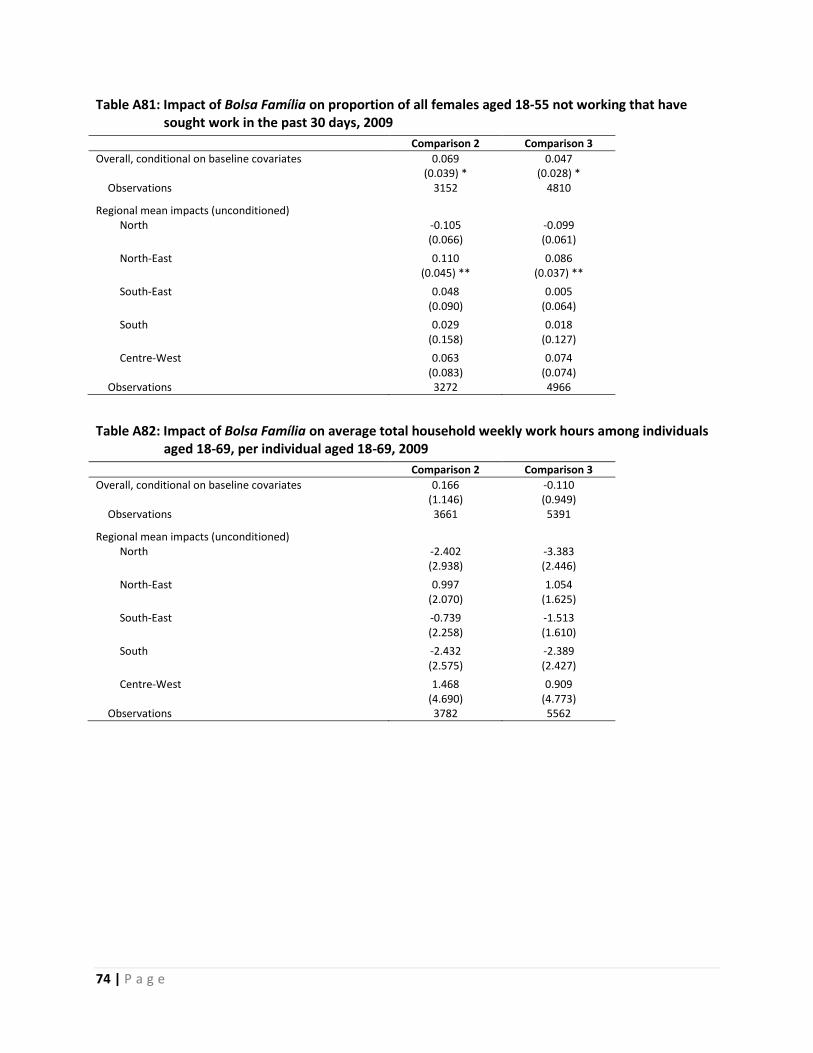
74 | P a g e
Table A81: Impact of Bolsa Família on proportion of all females aged 18-55 not working that have sought work in the past 30 days, 2009
Comparison 2 Comparison 3
Overall, conditional on baseline covariates 0.069 0.047
(0.039) * (0.028) *
Observations 3152 4810
Regional mean impacts (unconditioned) North -0.105 -0.099
(0.066) (0.061)
North-East 0.110 0.086
(0.045) ** (0.037) **
South-East 0.048 0.005
(0.090) (0.064)
South 0.029 0.018
(0.158) (0.127)
Centre-West 0.063 0.074
(0.083) (0.074)
Observations 3272 4966
Table A82: Impact of Bolsa Família on average total household weekly work hours among individuals aged 18-69, per individual aged 18-69, 2009
Comparison 2 Comparison 3
Overall, conditional on baseline covariates 0.166 -0.110
(1.146) (0.949)
Observations 3661 5391
Regional mean impacts (unconditioned) North -2.402 -3.383
(2.938) (2.446)
North-East 0.997 1.054
(2.070) (1.625)
South-East -0.739 -1.513
(2.258) (1.610)
South -2.432 -2.389
(2.575) (2.427)
Centre-West 1.468 0.909
(4.690) (4.773)
Observations 3782 5562

75 | P a g e
Table A83: Impact of Bolsa Família on average formal household weekly work hours among individuals aged 18-69, per individual aged 18-69, 2009
Comparison 2 Comparison 3
Overall, conditional on baseline covariates -7.980 -8.869
(1.512) *** (1.318) ***
Observations 3661 5391
Regional mean impacts (unconditioned) North -13.546 -10.757
(3.828) *** (3.901) ***
North-East -8.169 -8.037
(2.407) *** (2.140) ***
South-East -5.951 -6.318
(3.190) * (2.928) **
South -12.561 -15.709
(6.543) * (5.603) ***
Centre-West -4.291 -3.291
(5.833) (6.084)
Observations 3782 5562
Table A84: Impact of Bolsa Família on average informal household weekly work hours among individuals aged 18-69, per individual aged 18-69, 2009
Comparison 2 Comparison 3
Overall, conditional on baseline covariates 7.801 8.748
(1.710) *** (1.429) ***
Observations 3661 5391
Regional mean impacts (unconditioned) North 11.826 7.350
(3.990) *** (3.588) **
North-East 8.952 9.288
(2.976) *** (2.519) ***
South-East 5.064 4.775
(3.652) (3.155)
South 7.464 12.189
(6.130) (5.289) **
Centre-West 6.664 4.464
(7.966) (7.879)
Observations 3782 5562

76 | P a g e
Table A85: Impact of Bolsa Família on average total household weekly work hours among males aged 18-69, per male aged 18-69, 2009
Comparison 2 Comparison 3
Overall, conditional on baseline covariates -0.785 -0.384
(1.599) (1.336)
Observations 3432 5078
Regional mean impacts (unconditioned) North -3.580 -3.895
(4.403) (3.776)
North-East -1.133 0.667
(3.169) (2.299)
South-East -3.039 -4.388
(2.907) (2.380) *
South 2.632 0.797
(7.555) (6.095)
Centre-West -3.077 1.425
(6.867) (7.355)
Observations 3542 5237
Table A86: Impact of Bolsa Família on average total household weekly work hours among females aged 18-69, per female aged 18-69, 2009
Comparison 2 Comparison 3
Overall, conditional on baseline covariates 0.304 0.244
(1.495) (1.344)
Observations 3410 5066
Regional mean impacts (unconditioned) North -0.761 -1.050
(4.242) (3.865)
North-East 1.239 0.044
(2.742) (2.190)
South-East 3.047 3.791
(3.765) (2.812)
South -4.415 -2.891
(7.817) (6.373)
Centre-West 2.467 -1.464
(6.094) (7.427)
Observations 3527 5232

77 | P a g e
Table A87: Impact of Bolsa Família on average formal household weekly work hours among males aged 18-69, per male aged 18-69, 2009
Comparison 2 Comparison 3
Overall, conditional on baseline covariates -4.605 -4.697
(1.485) *** (1.136) ***
Observations 3432 5078
Regional mean impacts (unconditioned) North -9.547 -8.045
(3.717) ** (3.738) *
North-East -4.703 -4.321
(2.630) * (2.179) **
South-East -3.622 -4.688
(3.248) (2.841) *
South 4.144 1.920
(4.582) (3.158)
Centre-West -7.170 -6.456
(4.821) (5.698)
Observations 3542 5237
Table A88: Impact of Bolsa Família on average informal household weekly work hours among males aged 18-69, per male aged 18-69, 2009
Comparison 2 Comparison 3
Overall, conditional on baseline covariates 3.460 4.228
(1.483) ** (1.163) ***
Observations 3432 5078
Regional mean impacts (unconditioned) North 6.754 4.186
(4.191) (3.433)
North-East 3.273 4.989
(2.578) (1.982) **
South-East 0.547 0.355
(3.424) (3.320)
South -4.454 -2.432
(4.711) (4.344)
Centre-West 5.090 8.508
(8.143) (5.579)
Observations 3542 5237
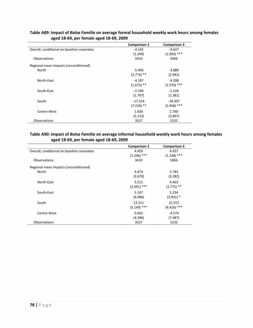
78 | P a g e
Table A89: Impact of Bolsa Família on average formal household weekly work hours among females aged 18-69, per female aged 18-69, 2009
Comparison 2 Comparison 3
Overall, conditional on baseline covariates -4.142 -4.627
(1.209) (1.093) ***
Observations 3410 5066
Regional mean impacts (unconditioned) North -5.496 -3.889
(2.774) ** (2.942)
North-East -4.187 -4.208
(1.673) ** (1.570) ***
South-East -2.240 -1.526
(1.797) (1.381)
South -17.524 -18.307
(7.220) ** (5.958) ***
Centre-West 1.830 2.760
(5.133) (3.897)
Observations 3527 5232
Table A90: Impact of Bolsa Família on average informal household weekly work hours among females aged 18-69, per female aged 18-69, 2009
Comparison 2 Comparison 3
Overall, conditional on baseline covariates 4.459 4.937
(1.296) *** (1.238) ***
Observations 3410 5066
Regional mean impacts (unconditioned) North 4.674 2.783
(3.670) (3.282)
North-East 5.511 4.463
(2.091) *** (1.775) **
South-East 5.167 5.234
(4.086) (2.831) *
South 13.311 15.557
(5.149) *** (4.416) ***
Centre-West 0.602 -4.574
(4.396) (7.487)
Observations 3527 5232

79 | P a g e
Table A91: Impact of Bolsa Família on proportion of total household weekly work hours among individuals aged 18-69 devoted to formal sector, 2009
Comparison 2 Comparison 3
Overall, conditional on baseline covariates -0.198 -0.219
(0.036) *** (0.031) ***
Observations 3616 5324
Regional mean impacts (unconditioned) North -0.217 -0.144
(0.076) *** (0.071) **
North-East -0.220 -0.218
(0.057) *** (0.053) ***
South-East -0.146 -0.140
(0.069) ** (0.063) **
South -0.278 -0.358
(0.168) * (0.143) **
Centre-West -0.105 -0.103
(0.148) (0.152)
Observations 3734 5492
Table A92: Impact of Bolsa Família on proportion of total household weekly work hours among individuals aged 18-69 worked by females, 2009
Comparison 2 Comparison 3
Overall, conditional on baseline covariates 0.021 0.025
(0.034) (0.029)
Observations 5129 7563
Regional mean impacts (unconditioned) North -0.023 -0.006
(0.056) (0.050)
North-East 0.055 0.033
(0.050) (0.040)
South-East 0.044 0.075
(0.062) (0.046)
South -0.133 -0.060
(0.174) (0.153)
Centre-West 0.120 0.004
(0.097) (0.119)
Observations 5288 7802
2.3.2 Social capital
We consider the following outcomes related to social capital: whether the household has membership
in any group and whether the household has membership in any group excluding church (Tables A93
through A96). Single-difference estimates using only 2009 data show no strongly significant impacts on
these social capital outcomes. Double-difference estimates for all groups using 2005 and 2009 data
show a small positive impact but this does not persist when church-based groups are excluded.

80 | P a g e
Table A93: Impact of Bolsa Família on membership in any group, 2009
Comparison 2 Comparison 3
Overall, conditional on baseline covariates 0.041 0.031
(0.033) (0.025)
Observations 5112 7541
Regional mean impacts (unconditioned) North 0.014 -0.004
(0.061) (0.051)
North-East 0.035 0.031
(0.060) (0.046)
South-East -0.034 0.006
(0.064) (0.050)
South 0.317** 0.203**
(0.113) (0.083)
Centre-West -0.052 0.003
(0.049) (0.043)
Observations 5238 7724
Table A94: Impact of Bolsa Família on change in membership in any group (Difference-in-Difference)
Comparison 2 Comparison 3
Overall, conditional on baseline covariates 0.083** 0.050*
(0.040) (0.033)
Observations 5238 7541
Regional mean impacts (unconditioned) North 0.017 -0.036
(0.083) (0.069)
North-East 0.086 0.036
(0.069) (0.051)
South-East 0.004 0.020
(0.082) (0.073)
South 0.264** 0.185*
(0.102) (0.097)
Centre-West 0.089 0.096
(0.115) (0.115)
Observations 5112 7724
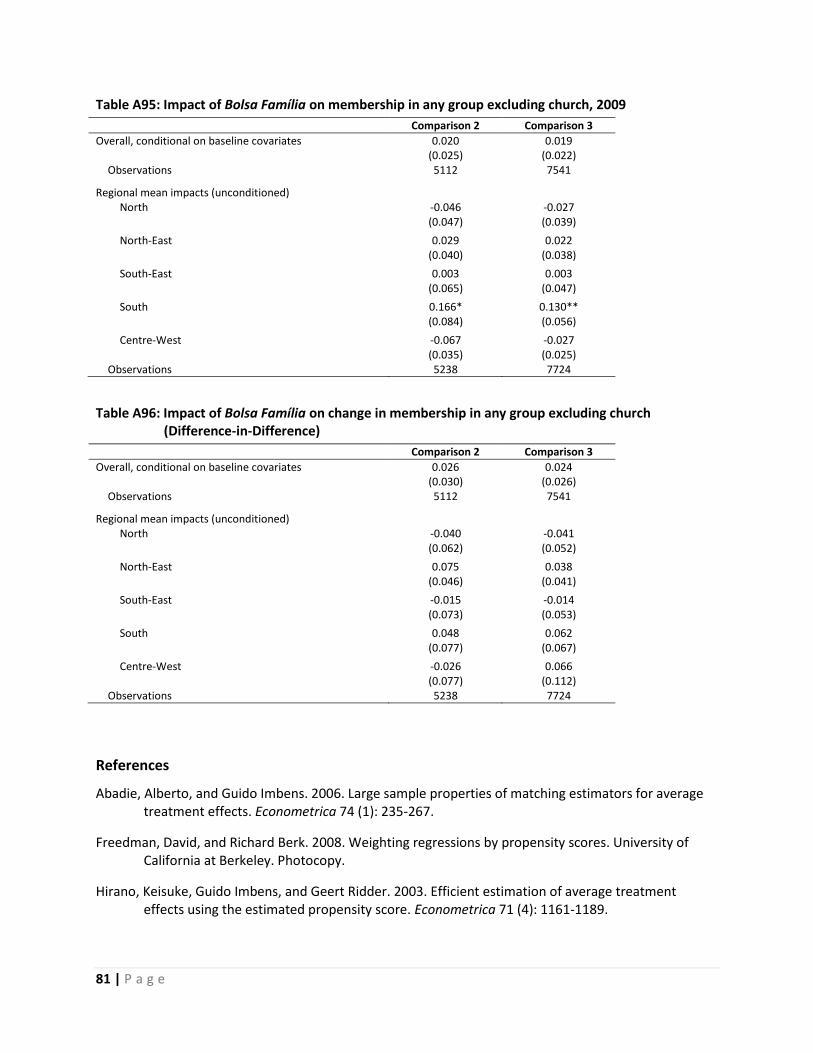
81 | P a g e
Table A95: Impact of Bolsa Família on membership in any group excluding church, 2009
Comparison 2 Comparison 3
Overall, conditional on baseline covariates 0.020 0.019
(0.025) (0.022)
Observations 5112 7541
Regional mean impacts (unconditioned) North -0.046 -0.027
(0.047) (0.039)
North-East 0.029 0.022
(0.040) (0.038)
South-East 0.003 0.003
(0.065) (0.047)
South 0.166* 0.130**
(0.084) (0.056)
Centre-West -0.067 -0.027
(0.035) (0.025)
Observations 5238 7724
Table A96: Impact of Bolsa Família on change in membership in any group excluding church (Difference-in-Difference)
Comparison 2 Comparison 3
Overall, conditional on baseline covariates 0.026 0.024
(0.030) (0.026)
Observations 5112 7541
Regional mean impacts (unconditioned) North -0.040 -0.041
(0.062) (0.052)
North-East 0.075 0.038
(0.046) (0.041)
South-East -0.015 -0.014
(0.073) (0.053)
South 0.048 0.062
(0.077) (0.067)
Centre-West -0.026 0.066
(0.077) (0.112)
Observations 5238 7724
References
Abadie, Alberto, and Guido Imbens. 2006. Large sample properties of matching estimators for average treatment effects. Econometrica 74 (1): 235-267.
Freedman, David, and Richard Berk. 2008. Weighting regressions by propensity scores. University of California at Berkeley. Photocopy.
Hirano, Keisuke, Guido Imbens, and Geert Ridder. 2003. Efficient estimation of average treatment effects using the estimated propensity score. Econometrica 71 (4): 1161-1189.