The Identity of Zeros of Higher and Lower Dimensional Filter Banks and TheConstruction of Multidimensional Nonseparable Wavelets

A dissertation submitted in partial fulfillment of the requirements for the degree ofDoctor of Philosophy at George Mason University

By

Sirak BelaynehMaster of Science

George Mason University, 1990Bachelor of Science

Addis Ababa University, 1976

Director: Professor Edward J. WegmanSchool of Information Technology and Engineering

Fall Semester 2008George Mason University

Fairfax, VA

ii

DEDICATION

Dedicated to my daughters Meron and Mekedas who bring love and joy to my world andin memory of my parents Ayelech Tessema, Belayneh Woldeyes, my sister AsterBelayneh and my friend Nolawi Abebe.

iii

ACKNOWLEDGEMENTS

I would like to express my deepest appreciation to my advisor, Professor EdwardWegman, for his friendship, his excellent advise through all my graduate study. I am alsovery thankful to members of my defense committee, Professor Stephan Nash, ProfessorDavid Walnut, Professor Kristine Bell and Professor Yasmin Said for their time andassistance in reviewing my dissertation.

I also would like to thank Professor Daniel Menasce, Lisa Nodler and Laura Harrison ofthe Dean's office for their cooperation and encouragement.

Finally I would like to thank my wife, Fikirte Worku, my relatives and friends who stoodby me and encouraged me through the years. Special thanks also go to my brother Eliasfor his encouragement and support.

iv

TABLE OF CONTENTS

PageList of Figures…………………………………………………………………………....viiList of Abbreviations and Symbols....................................................................................ixAbstract................................................................................................................................x

CHAPTER 1: INTRODUCTION.....................................................................................1 1.1 Overview............................................................................................................1 1.2 Problem Statement and Motivation...................................................................2 1.3 Overview of the Dissertation.............................................................................3

CHAPTER 2: WAVELETS, MRA AND FILTER BANKS..........................................6 2.1 Introduction........................................................................................................6 2.2 From Fourier Analysis to Wavelet Analysis......................................................6 2.2.1 Fourier Analysis..................................................................................6 2.2.2 Gabor Transform.................................................................................8 2.2.3 Short-Time Fourier Transform (STFT)..............................................9 2.2.4 Wavelets............................................................................................10 2.3 Multiresolution Analysis..................................................................................14 2.4 Multirate Filter Banks......................................................................................17 2.4.1 Multirate............................................................................................17 2.4.1.1 Down-Sampling.................................................................18 2.4.1.2 Up-Sampling......................................................................19 2.4.2 Perfect Reconstruction Filter Bank...................................................21 2.4.3 Two Channel PRFB..........................................................................22 2.4.3.1 Time Domain Analysis......................................................23 2.4.3.2 Polyphase Domain Analysis..............................................24 2.4.3.3 Modulation Domain Analysis............................................26 2.5 Unified Approach.............................................................................................26 2.5.1 Wavelet and MRA............................................................................27 2.5.2 Filter Bank and MRA......................................................................29 2.5.3 Filter Bank and Wavelet...................................................................29 2.6 Summary..........................................................................................................31

CHAPTER 3:MULTIDIMENSIONAL EXTENSION.................................................32 3.1 Introduction......................................................................................................32 3.2 Preliminaries....................................................................................................32

v

3.2.1 Multidimensional Sampling..............................................................32 3.2.1.1 Down Sampling and Decimation...................................................35 3.2.1.2 Upsampling and Interpolation.......................................................38 3.2.2 Polyphase Decomposition.................................................................40 3.2.3 Examples ................................................................................41 3.3 Multidimensional Filter Banks........................................................................48 3.3.1 Modulated Analysis..........................................................................49 3.3.2 Polyphase Analysis...........................................................................51 3.3.3 Additional Constraints......................................................................55 3.3.3.1 Orthogonal Case................................................................55 3.3.3.2 Linear Phase.......................................................................56 3.3.4 Examples ................................................................................58 3.4 Synthesis of Multidimensional Filter Banks....................................................61 3.4.1 Numerical Optimization....................................................................61 3.4.2 Cascade.............................................................................................62 3.4.2.1 Orthogonal.........................................................................63 3.4.2.2 Linear Phase.......................................................................64 3.4.2.3 Example.............................................................................64 3.4.3 to Order Filter.........................................................................69N-1 N 3.4.3.1 Example.............................................................................70 3.4.4 Transformation..................................................................................73 3.4.4.1 Separable Polyphase Components.....................................73 3.4.4.2 McClellan Transformation.................................................77 3.4.4.3 Example.............................................................................77 3.5 Summary..........................................................................................................80

CHAPTER 4:REGULARITY CONDITION................................................................82 4.1 Introduction......................................................................................................82 4.2 Regularity.........................................................................................................82 4.3 Two-Channel Case ................................................................................89 4.3.1 Example............................................................................................91 4.4 Construction of Regular Cascade Filters.........................................................97 4.4.1 Example............................................................................................98 4.5 Summary........................................................................................................100

CHAPTER 5:MULTIDIMENSIONAL WAVELETS...............................................102 5.1 Introduction....................................................................................................102 5.2 Tensor Product of One-Dimensional Basis...................................................102 5.2.1 Tensor Product of One-Dimensional Wavelets..............................102 5.2.2 Tensor Product of One-Dimensional MRA....................................103 5.3 General MRA Construction ..................................................................105 5.4 Wavelet Bases From Iterated Multidimensional Filter Banks.......................106 5.5 Design of Compactly Supported Wavelets....................................................110

vi

5.5.1 Direct Design..................................................................................110 5.5.2 Indirect Design from Known One-Dimensional Wavelets.............116 5.6 Summary........................................................................................................120

CHAPTER 6:APPLICATION IMAGE RESTORATION.......................................121 6.1 Introduction....................................................................................................121 6.2 Preliminaries..................................................................................................121 6.3 Image Restoration and Reconstruction..........................................................123 6.3.1 Source of Image Degradation.........................................................125 6.3.2 Some Classical Image Restoration Techniques..............................126 6.3.3 Wavelets and Image Restoration....................................................127 6.4 Simulation......................................................................................................129 6.4.1 Image Reconstruction.....................................................................130 6.4.1.1 2-D Images......................................................................130 6.4.1.2 3-D Image.......................................................................133 6.4.2 Image Denoising..........................................................................135 6.6 Summary........................................................................................................138

CHAPTER 7:CONCLUSION AND FUTURE WORK.............................................139 7.1 Conclusions....................................................................................................139 7.2 Future Research.............................................................................................141

APPENDIX A................................................................................................................143

APPENDIX B................................................................................................................145

APPENDIX C................................................................................................................148

LIST OF REFERENCES..............................................................................................151

vii

LIST OF FIGURES

Figures Page 2.1 STFT & WAVELET..............................................................................................132.2 Multiresolution analysis.........................................................................................142.3 Downsampling.......................................................................................................192.4 Upsampling............................................................................................................202.5 Multirate Filter Bank.............................................................................................212.6 Two Channel PRFB...............................................................................................232.7 Iterated Filter Bank................................................................................................293.1 Multidimensional Sampling Lattice.......................................................................333.2 Multidimensional Sampling Lattice & Cosets.......................................................343.3 Multidimensional Sampling Downsampler...........................................................363.4 Multidimensional Sampling Upsampler................................................................393.5 Frequency Domain Baseband Change...................................................................403.6 Bases Vectors and Fundamental Cell....................................................................423.7 Example of Aliasing Frequencies For D................................................................433.8 Admissible Passbands Generated by D.................................................................443.9 Coset Vectors Generated by FCO Sampling.........................................................453.10 Baseband and Aliasing Frequency FCO Sampling................................................463.11 Admissible Passband for the FCO Sampling........................................................473.12 Multidimensional PRFB........................................................................................493.13 Multidimensional Analysis/Synthesis Filter Bank................................................533.14 Multidimensional Two Channel PRFB..................................................................583.15 3-D FCO HP & LP Filters.....................................................................................724.1 Extension from One to Multiple Dimension..........................................................985.1 Multidimensional Iterated Filter Bank.................................................................1075.2 Scaling Function..................................................................................................1125.3 Daubechie's Wavelet............................................................................................1135.4 2-D Scaling Function...........................................................................................1145.5 2-D Wavelet Function..........................................................................................1156.1 Image degradation module and restoration process.............................................1246.2 Basic Image resolution module............................................................................1286.3 Image Reconstruction 2nd order nonseparable filter...........................................1306.4 Image Reconstruction 3rd order nonseparable filer.............................................1316.5 Image Reconstruction 2nd order separable filer..................................................1326.6 Image Reconstruction 3rd order separable filer...................................................1336.7 Original 3-D flow.................................................................................................134

viii

6.8 Reconstruction 3-D flow......................................................................................1356.9 Image Denoise 2nd order nonseparable filter......................................................1366.10 Image Denoise 2nd order separable filter............................................................137

ix

LIST OF ABBREVIATIONS AND SYMBOLS

AC Analysis Component BSNR Blurred Signal-To-Noise Ratio CWT Continuous-time Wavelet Transform DCT Discrete Cosine Transform DFT Discrete Fourier Transform FCO Face Centered orthorhombic FFT Fast Fourier Transform FIR Finite Impulse Response FPT Forward Polyphase Transform FS Fourier Series IPT Inverse Polyphase Transform ISNR Improvement to Signal-To-Noise Ratio MRA Multiresolution Analysis MRFB Multirate Filter Bank MRI Magnetic Resonance Imaging MSE Mean Square Error ON Orthonormal PR Perfect Reconstruction PRFB Perfect Reconstruction Filter Bank QAR Quantitative Autoradiology QM Quadratic Mirror QMF Quadratic Mirror Filter R-function Reisz function SC Synthesis Component SNR Signal to Noise Ratio S.O. Semi Orthogonal STFT Short-Time Fourier Transform WS Wavelet Series WT Wavelet Transform

ABSTRACT

THE IDENTITY OF ZEROS OF HIGHER AND LOWER DIMENSIONALFILTERBANKS AND THE CONSTRUCTION OF MULTIDIMENSIONALNONSEPARABLE WAVELETS

Sirak Belayneh, Ph.D.

George Mason University, 2008

Dissertation Director: Prof. Edward J. Wegman

This dissertation investigates the construction of nonseparable multidimensional

wavelets using multidimensional filterbanks. The main contribution of the dissertation is

the derivation of the relations zeros of higher and lower dimensional filtersbanks for

cascade structures. This relation is exploited to construct higher dimensional regular

filters from known lower dimensional regular filters. Latter these filters are used to

construct multidimensional nonseparble wavelets that are applied in the reconstruction

and denoising of multidimensional images.

The relation of discrete wavelets and multirate filterbanks was first demonstrated

by Meyer and Mallat. Latter, Daubechies used this relation to construct continuous

wavelets using the iteration of filterbanks. Daubechies also set the necessary conditions

on these filer banks for the construction of continuous wavelets. These conditions also

known as the regularity condition are critical for the construction of continuous wavelet

basis form iterated filterbanks.

In the single dimensional case these regularity conditions are defined in terms of

the order of zeros of the filterbanks . The iteration of filterbanks with higher order zeros

results in fast convergence to continuous wavelet basis. This regularity condition for the

single dimensional case has been extended by Kovachevic to include the

multidimensional case. However, the solutions to the regularity condition are often

complicated as the orders and dimensions increase.

In this dissertation the relations of zeros of lower and higher dimensional filters

based on the definition of regularity conditions for cascade structures has been

investigated. The identity of some of the zeros of the higher and lower dimensional

filterbanks has been established using concepts in linear spaces and polynomial matrix

description. This relation is critical in reducing the computational complexity of

constructing higher order regular multidimensional filterbanks. Based on this relation a

procedure has been adopted where one can start with known single dimensional regular

filterbanks and construct the same order multidimensional nonseparable regular

filterbanks . These filterbanks are then iterated as in the one dimensional case to give

continuous multidimensional nonseparabke wavelets. The conditions for dilation

matrices with better isotropic transformation has also been revisited. Several examples

are used to illustrate the construction of these multidimensional nonseparable wavelets.

Finally, these nonseparable multidimensional wavelet basis are used in the reconstruction

and denoising of multidimensional images and the results are compared to those obtained

by separable wavelets.

1

CHAPTER 1

INTRODUCTION

1.1 Overview

In the last two decades three quite independently developed concepts in the areas

of applied mathematics, signal processing and computer vision have emerged into one

unified theory. In applied mathematics, dilation and translation have been used for long

time to generate families of functions from single prototype function. Fourier analysis

and more recently wavelet analysis are such examples. The works of A. Grossman and J.

Morlet grew to what is known today as wavelets [28]. In the area of signal processing,

the concept of multirate filter banks evolved from the simple idea of splitting signals into

channels so as to be able to reconstruct them without spectral overlap (aliasing) [7], [59].

A. Croisier, D. Esteban and C. Galand first observed the phenomena in 1976 [18].

Subsequently, F. Mintzer, M. J. T. Smith and T. P. Barnwell [2], [57], [71], [72], [82]

developed the idea of perfect reconstruction filter banks (PRFB). In computer vision, the

concept of multiresolution analysis developed as a method of successive refinement of

signals or pyramidal coding schemes [1], [8], [33]. S. Mallat and Y. Meyer [51], [52],

[56] used the concept of MRA to arrive at octave band splitting.

The connection between wavelet analysis, multirate filtering and multiresolution

analysis was gradually established. Mallat and Meyer [51], [56] were the first to show

such relation when they used the concept of MRA to arrive at octave band splitting in the

late eighties. Later Daubechies established the relation between the compactly supported

2

wavelet basis and iterated low pass branch of a particular subband scheme [21], [22].

Since then much research has been done to lay a firm theoretical bases for the unified

approach, which in turn has contributed to the refinement of techniques in the individual

areas [80]. For example concepts used to develop non-separable multidimensional filter

banks are applied to develop nonseparable wavelet basis.

1.2 Problem Statement and Motivation

My work is primarily motivated by the desire to understand the fine work of

Daubechies, Vetterli and Kovachevic and applying the concepts to multidimensional

image reconstruction [20], [85], [38], [36]. Later the work focused on solving the

problem posed by J. Kovachevic and M. Vetterli [39] of establishing the relation between

the zeros of higher and lower dimensional regular filters. This question has not been

addressed previously. Establishing the above relation contributed to the idea of

constructing higher dimensional filter from lower dimensional filters.

The goal of this dissertation was to extend some of the concepts pertaining to the

construction of wavelets from iterated filter banks to multiple dimensions. These include:

* establishing the relation of regularity condition of lower and higher dimensional

filters.

*developing methods for the construction of regular multidimensional filter banks

starting from known lower dimensional regular filter banks using the above

relation.

* constructing multidimensional nonseparable wavelet basis using the method of

iteration and the above constructed filter banks.

*setting the conditions on dilation matrices for better isotropic transformation

* applying the above wavelets for the reconstruction and denoising of

3

multidimensional images.

Substantial effort has been made to achieve all of the above stated goals. The

nonseparable wavelets have been used for the reconstruction and denoising of 2-D

images. The results show a more isotropic treatment of images than the separable

wavelets. However, the extension of the result to 3-D images has been computationally

cumbersome and required additional research in 3-D convolution and programming skills

for the manipulation of 3-D data.

1.3 Overview of the Dissertation

The first part of this thesis will concentrate on reviewing the basic concepts of

wavelet analysis, multirate filter banks and multiresolution analysis. A brief description

of the basic tenet and historical evolution of these three concepts are made. The concept

of Fourier analysis and its limitations that lead to the evolutionary transformation to

wavelet analysis are discussed. The mathematical concepts underlying wavelet analysis

are described. The fundamental theorems in multiresolution analysis and the concept of

successive approximation or refinement in signal processing is summarized. Finally, the

section ends with the discussion of basic concepts in multirate filter bank such as

sampling rate change and perfect reconstruction. The different techniques of analysis and

synthesis of perfect reconstruction filter banks are described.

The second part discusses the interrelationship of the above concepts and the

evolution of these relations into a unified theory in the one-dimensional case. An outline

derivation of one concept based on the assumptions of another is made. Special attention

is given to the construction of wavelet basis from iterated filter banks and the regularity

condition.

4

The third part discusses the extension of the above concepts to more than one

dimensions. The final objective is to extend the concept of one-dimensional construction

of continuous wavelets form iterated filter banks to multiple dimensions. The method of

constructing multidimensional wavelet basis based on the iteration of regular,

multidimensional nonseparable filter banks will be of special significance. This requires

basic knowledge of the fundamentals and techniques of construction of multidimensional

filter banks [92], [93]. All of the single dimensional concepts such as downsampling

perfect reconstruction filter banks and so on will be revisited with the aim of extending

them to multiple dimensions. Extension of these concepts requires a definition of a whole

series of new concepts that are widely different from those in the single dimensional case.

First these new concepts such as lattice, separability, coset vectors and so on which are

specific to multidimensional filters are elaborated. Even those common in one dimension

such as down and upsampling and perfect reconstruction are redefined within the

multidimensional frame.

The fourth part which is the core of this dissertation, discusses regularity of filter

banks. As in the one-dimensional case the construction of multidimensional wavelets

heavily depends on the construction of regular multidimensional filer banks. First the

basic definition of regularity is extended to multiple dimensions. Then the existence of

the relations of the zeros in the lower and higher dimensional filter banks are proved.

This relation between lower dimensional and higher dimensional cascade filters is then

used to construct higher dimensional regular filters from lower dimensional ones in the

next section.

The fifth part discusses the different alternative methods of construction of

multidimensional wavelets. The main emphasis will be on the construction of

multidimensional wavelets using the iteration method. The regular multidimensional

5

filter banks constructed above will be used to build nonseparable multidimensional

wavelets.

The six part will deal with image reconstruction and denoising algorithms and

the special advantages of using the multidimensional nonseparable wavelet transform.

The nonseparable multidimensional wavelet basis constructed above will be used to

reconstruct and denoise multidimensional images. In this section illustrative examples are

used used to demonstrate the concepts.

The final section summarizes the results and contributions as well as proposals for

future work.

6

CHAPTER 2

WAVELETS, MRA and FILTER BANKS

2.1 INTRODUCTION:

The background knowledge essential to the understanding of this research is

outlined in this section. The basic concepts of wavelet analysis, multiresolution analysis

and multirate filter banks and the interconnection between them are fundamental in the

construction of the multidimensional wavelet bases. It is essentially these concepts that

will be latter extended to construct the multidimensional wavelet bases. The material in

this chapter is based on the literature and fine works of C. K. Chui, I. Daubechies, M.

Vetterlli and J. Kovacevic, Y. Meyer , E. Viscito and others [15], [21], [85], [56], [87]Þ

I start by reviewing essential concepts from discrete-time signal processing

theory. Then a brief look of each of the above three concepts along with their historical

evolution is made.

2.2 FROM FOURIER TO WAVELET TRANSFORM:

2.2.1 FOURIER ANALYSIS:

Fourier analysis has been the foundation of harmonic analysis and constitutes two

components, Fourier transform and Fourier series. The Fourier transform of aF

measurable function is defined asf

2.1F( ) = f(x) e dx= '02 -nix1

7

The Fourier transform has limitations in the study of the spectral behavior of

analog signal. First, full knowledge of the signal in the time-domain is required and

second if the signal is nonstationary the entire spectrum is affected.

The Fourier series representation of any in is given by f L (0,2 )21

2.2c = f(x)e dx n1

2 02 -inx

1

1'

where the constants are the Fourier coefficients of and are defined byc f n

2.3 f(x) = c e . -

inx

∞

∞

n

denotes the collection of measurable functions defined on the intervalL (0,2 ) f2 1

(0,2 )1 with

f(x) dx < . 2.4'021l l ∞

The Fourier series representation has two distinct features. First the function isf

decomposed into the sum of infinitely many mutually orthogonal components g (x) =n

c e (x) = e L (0,2 )n ninx inx 2 since form orthonormal basis of . The second distinct feature= 1

is that the orthogonal basis is generated by dilation of an angle function .=n =(x) = eix

The Fourier series representation also satisfies the Parseval identity indicating

that to be isometric to each other.l (0,2 ), L (0,2 )2 21 1

2.5 12 0

2

n=-n

21

1' l l l lf(x) dx = c 2

∞

∞

8

Let us now consider measurable functions in . Since every function in L (R) L (R)2 2

must decay to zero at the sinusoidal functions do not belong to .„∞ =838BÐBÑ œ / L (R)2

The wavelets that generate must on one hand have fast decay and on the other< L (R)2

hand must cover the whole real line.

The above limitation of Fourier analysis lead to the development of the following

transforms.

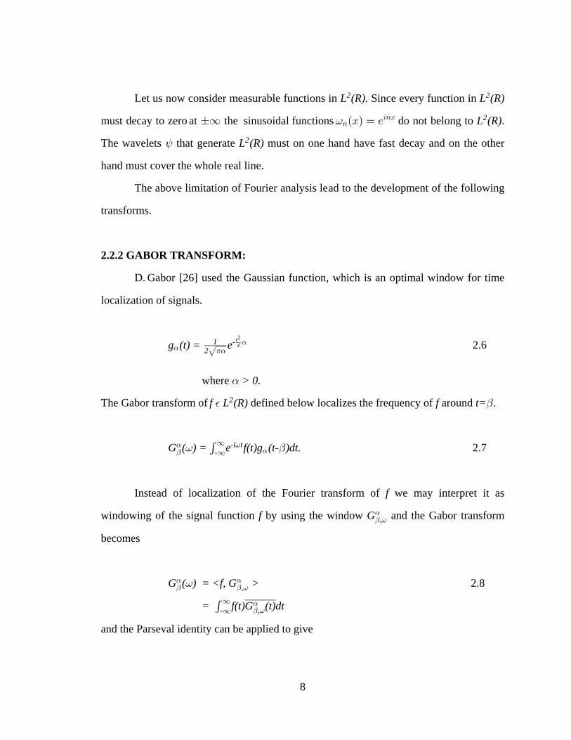
2.2.2 GABOR TRANSFORM:

D. Gabor [26] used the Gaussian function, which is an optimal window for time

localization of signals.

2.6g (t) = eα 1αα1

2-È t2

4

where α > 0.

The Gabor transform of defined below localizes the frequency of around .f L (R) f t=% "2

2.7G ( ) = e f(t)g (t- )dt."α =

α= "'-

-i t∞∞

Instead of localization of the Fourier transform of we may interpret it asf

windowing of the signal function by using the window and the Gabor transformf G" =α

,

becomes

2.8G ( ) = <f, G >" " =α α= ,

= f(t)G (t)dt'- ,∞∞

" =α

and the Parseval identity can be applied to give

9

2.9<f, G > = <f , G > " =α

1 " =

α

,1

2 ,s s

G ( ) = G (- ). 2.10"α

1α= "e

2-i 1

4"=

=αÈ

The window Fourier transform of with window at agrees with thef g t=α "

"window inverse Fourier transform" with window at . The product of these twog4

1α (=0

windows would give the area of the time-frequency window.

(2 )(2 ) = 2 2.11? ?gαα

g14

<f, G > = <f , H >" = " =α α

, ,s

where H ( ) = e ( - )." =α "(

1α α,e

2-i g

4( ( =Š ‹i1

"=È In general any window function can be defined, but must satisfy the=

requirement

2.12t (t) L (R)= % 2

and also

2.13l lt (t) L (R)."#= % 2

2.2.3 SHORT-TIME FOURIER TRANSFORM (STFT):

If is chosen such that and its Fourier transform satisfy the above= % = L (R)2 =s

condition, then the window Fourier transform called STFT of is defined as follows withf

rigid window at .t=b

2.14F( ) = e f(t) (t-b)dt= ='-

-i t∞∞ =

and satisfy= =s

. 2.15? ?= = s"# 

10

The optimal window is obtained when we have the equality. The Gabor transform

with the Gaussian window is STFT with the smallest time-frequency window. The Gabor

transform does not give extra freedom to achieve other desirable properties, which a

larger window can give. The larger window gives extra degree of freedom for

introducing dilation to make time-frequency window flexible.

The analysis of signals using STFT gives a time-frequency window that is still

rigid. It does not give the flexibility to adjust the time window based on the frequency.

Normally a narrow time-window is required to locate high frequency phenomena

precisely and wide time-window to analyze low frequency signals.

Thus to overcome this resolution limitation of STFT , the basic wavelet is? ?t f

defined with the flexibility of time-frequency window, which narrows automatically with

high frequency phenomena and widens otherwise. This is possible by making ?f

proportional to the central window frequency that is f

. 2.16?ff = c

2.2.4 WAVELETS:

The limitation in the rigidity of the time-frequency window of STFT forced the

introduction of the integral wavelet transform. Instead of windowing the Fourier and

inverse Fourier transform as in the STFT, the integral wavelet transform windows the

function and its Fourier transform directly allowing flexibility of the time-frequency

window using dilation parameters.

The integral wavelet transform is defined in terms of the basic wavelet G% L (R)2

as

, 2.17W f(b,a) = a f(t) ( ) dtG k k '-12

∞∞

G t-ba

11

where is a basic wavelet if and satisfies the admissibility conditionG G% L (R)2

2.18C = < . GG =

='

-( )

∞∞ s¸ ¸k k

#

∞

If and satisfy the admissibility condition, then the basic wavelet providesG G Gs

the time-frequency window with area . Under the assumptions mentioned above4?G?Gs

G G is a continuous function and from the finiteness of equation 2.18 orC (0)G

2.19'-∞∞G(t)dt = 0.

Thus the basic wavelet is defined asG

, 2.20G Gb,t(t-b)

a(t) = a ( )k k -12

and the wavelet transform is given by

. 2.21W f(b,a) = <f , >G Gb,a

can be used as a basic wavelet only if the inversion exists. The function has toG f

be reconstructed from the values of . Any formula that expresses every W f(b,a) f L (R)G % 2

in terms of is called Inversion Formula and the kernel function to be used inW f(b,a)G Gs

this formula will be called a dual of the basic wavelet . The recovery of from G f W fG

depends on the domain of . The conditions of recovery of for the special dyadic(a,b) f

case where , , and are covered under Reisz basis (see Appendix A).b=k/2 a=1/2 j, k Zj j %

12

An R-function (Reisz function) is called an R-wavelet (wavelet) if thereG % L (R)2

exists a function such that and are dual bases of . If is anG % G G G~ L (R) { } { } L (R)2 j,k 2

j,k

R-wavelet, then is called dual wavelet corresponding to .~G G

Every wavelet orthogonal or not generates a wavelet series representation ofG

any ,f L (R)% 2

, 2.22f(x) = C (x)j,k=-

j,k j,k∞

G

where is the wavelet transform of relative to the dual .~C fj,k G

If is an orthogonal wavelet the decomposition is also orthogonal and unique.G

However, there are class of wavelets called semi-orthogonal that can be used to{ }Gj,k

generate without requiring the orthonormal properties for each , that isL (R) j2

2.23< , > = .G G $j,k j,l k,l

A wavelet in is called semiorthonormal (s.o.) wavelet if the Reisz basisG L (R)2

{ }Gj,k it generates satisfies

. 2.24< , > = 0 j l , j,k,l,m ZG G %j,k l,m Á

Every semiorthonormal wavelet generates orthogonal decomposition of ,L (R)2

and if is nonorthogonal wavelet (not s.o.) being Reisz basis has a dual and the pair~G G

{ , }~G G satisfies the biorthogonal properties

13

2.25< , > = j,k,l,m Z.G G $ $ %j,k l,m j,l k,m

This can be used to generate biorthogonal decomposition of , and is used toL (R)2

construct linear phase filter banks.

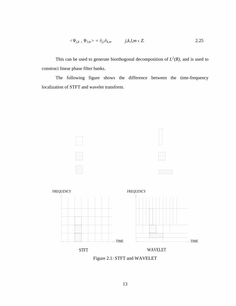
The following figure shows the difference between the time-frequency

localization of STFT and wavelet transform.

FREQUENCY FREQUENCY

TIME TIME

STFT WAVELET

Figure 2.1: STFT and WAVELET

14

2.3 MULTIRESOLUTION ANALYSIS:

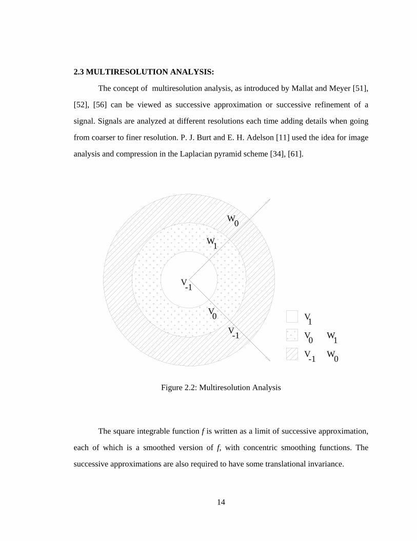
The concept of multiresolution analysis, as introduced by Mallat and Meyer [51],

[52], [56] can be viewed as successive approximation or successive refinement of a

signal. Signals are analyzed at different resolutions each time adding details when going

from coarser to finer resolution. P. J. Burt and E. H. Adelson [11] used the idea for image

analysis and compression in the Laplacian pyramid scheme [34], [61].

V1V0V-1

W1W0

V-1

V0V-1

W1

W0

Figure 2.2: Multiresolution Analysis

The square integrable function is written as a limit of successive approximation,f

each of which is a smoothed version of , with concentric smoothing functions. Thef

successive approximations are also required to have some translational invariance.

15

In general the multiresolution analysis consists of

1. embedded closed subspaces ,V L (R), m Zm § # %

2. such that

2.26+m Z

V =0%

m

V ,- mm Z

= L (R)%

#

3. and if is in the space then is in f(t) V f(2t) Vm m-"

, 2.27f(t) V f(2.t) V% %m m-1Í

4. Finally, there exists a such that for all , constitutes anF % % F V m Z0 mn

unconditional basis for , withVm

2.28V = span { } n Zm mnF %

and there exists such that for all , such that0<A B< C , n ZŸ ∞ n %

. 2.29A C C B Cn n n

n n mn n2 2 2l l Ÿ m m Ÿ l lF

If denote the orthogonal projection onto , thenP Vm m

2.30 P f = f for all f L (R).limm mÄ∞

#%

16

The successive projections as increases correspond to approximations of P f m fm

on a finer and finer scale.

Let us now define to be the orthogonal complement of in W , j Z V Vj j j-1%

2.31V = V Wj-1 j jŠ

and

2.32W W , if j j'.j j'¼ Á

Since and if and W V W j > j' j < Jj j' j'§ ¼

2.33V = V W ,J-j-1

k=0j J J-kŠ 9

which implies the decomposition of into mutually orthogonal subspaces, i.e.L (R)2

2.34L (R) = W .j Z

2j9

%

Furthermore inherits the scaling property of W Vj j

. 2.35f W f(2 ) W% %j 0jÍ

As with , there exists a vector such that its integer translates span , that isV W0 0G

. 2.36W = {span{ }0 0nG

From the scaling property above it follows

. 2.37W = {span{ }m mnG

17

Once the existence of is shown, it remains to construct this function. In theG

sequel the general construction of orthonormal wavelet basis is outlined.

A function with an orthonormal basis for is determined. BecauseF F F %0n 0V

V V =span{ (2x-n)} h0 -1 n§ F , there exists such that

2.38F F(x) = h (2x-n)n

n

and by definition

G F(x) = (-1) C (2x+n)n

nn-1

= g (2x+n).n

nF

These equations are called the "two-scale relations" of the scaling and wavelet

functions. The corresponding and will constitute an orthonormal basis of G G0n mn 0W

and respectively. constitutes an orthonormal wavelet basis for .W { , m,n Z} L (R)m mn2G %

The two scale sequences and defined above are the only quantities needed toh gn n

produce the coefficients of a wavelet multi-resolution decomposition.

2.4 MULTIRATE FILTER BANK

2.4.1 Multirate

In many applications of digital signal processing, it is necessary to make changes

in the sampling rate of a signal. One common example is the frequency conversion

between television standards (60 Hz US and 50 Hz European). Systems that employ

multiple sampling rates in the processing of digital signals are called multirate systems.

The process of sampling rate conversion in the digital domain can be viewed as a linear

filtering operation. Let us consider the two basic sampling rate conversions.

18

2.4.1.1 Down-Sampling

The first is down-sampling by a factor called decimation where every thD D

sample of the discrete sequence is kept and the rest is discarded. Its input/outputx(n)

relation is given by

2.3y(n) = x(Dn). *

In the Fourier and this relationship can be written as followsZ-domain

2.4Y( ) = Xs s= 1 -2 kD D

k=0

D ˆ ‰= 1 !

2.Y(z) = X(W z ).1D

k=0Dk 1

D %"

The down sampler is a linear, but periodically shift-varying operation as shown

on Figure 2.3. To avoid aliasing, we must first reduce the bandwidth of to = x(n) =max. D1

before down-sampling.

19

D

ALIASING

Figure 2.3: Downsampling

2.4.1.2 Up-Sampling

The second is up-sampling by a factor called interpolation where zeroesU U-1

are introduced between each successive values of the input signal . If input/outputx(n)

relationship is given by

if 2.y(n) = x( ) n = UknU %#

= 0 .if n Uk, k=0,1,Á á

The Fourier and -transform of the relations are given byz

2.Y( ) = X (U )s s= = %$

Y(z) = X(z ).U

20

From Figure 2.4 we see the production of the signal at points in the2k /U1

spectrum. To remove the unwanted images one would need a filter with the cut-off

frequency to follow the up-sampler.1U

U

Figure 2.4: Upsampling

For the general case of sampling-rate conversion by a rational factor , a cascadeUD

of the above two basic blocks can be used. The sampling rate conversion is achieved by

first performing interpolation by the factor and then decimation of the output of theU

interpolator by the factor . The filters can be combined to a single filter with cut-offD

frequency that is prevent aliasing and multiple imaging. There are severalmin( , )1 1U D

kinds of filter realizations of a decimator and interpolator and it is essential to consider

the efficiency of these filters in the design process. [63]Þ

21

2.4.2 Perfect Reconstruction Filter Bank

Subband systems consist of three components: analysis, transmission and

synthesis as shown below.

Figure 2.5: Multirate Filter Bank

The analysis section decomposes the signal into subband components and eachN

subband component is formed by filtering and resampling according to their

corresponding Nyquist frequency. The signal is then coded and transmitted. At the

synthesis section both up-sampling and filtering is done to reconstruct an approximation

to the input signal.

22

The aim in filter bank system design is to achieve perfect reconstruction by

eliminating distortions. The first distortion is due to aliasing arising from the down-

sampling of signals that are not perfectly band limited. The second is phase and

magnitude distortion. These distortions are eliminated by imposing design constraints on

both the analysis and synthesis filters. Aliasing in the sub-band components of the

analysis bank can be exactly canceled at the output of the synthesis bank by appropriately

choosing the synthesis filter. Some restrictions on the analysis filters are necessary if

certain properties such as FIR or stability conditions are to be desired. Other criteria are

imposed on the design of the analysis and synthesis filters in order to eliminate phase and

magnitude distortion allowing the output to be exact replica of the input within time shift

and scaling.

2.4.3 Two Channel PRFB

In what follows construction and analysis of two-channel filter bank is used to

demonstrate the above principles. Several methods are used to analyze the two-channel

PRFB, which is a special case of the -channel case and the methods can be extended toN

the -channel case.N

23

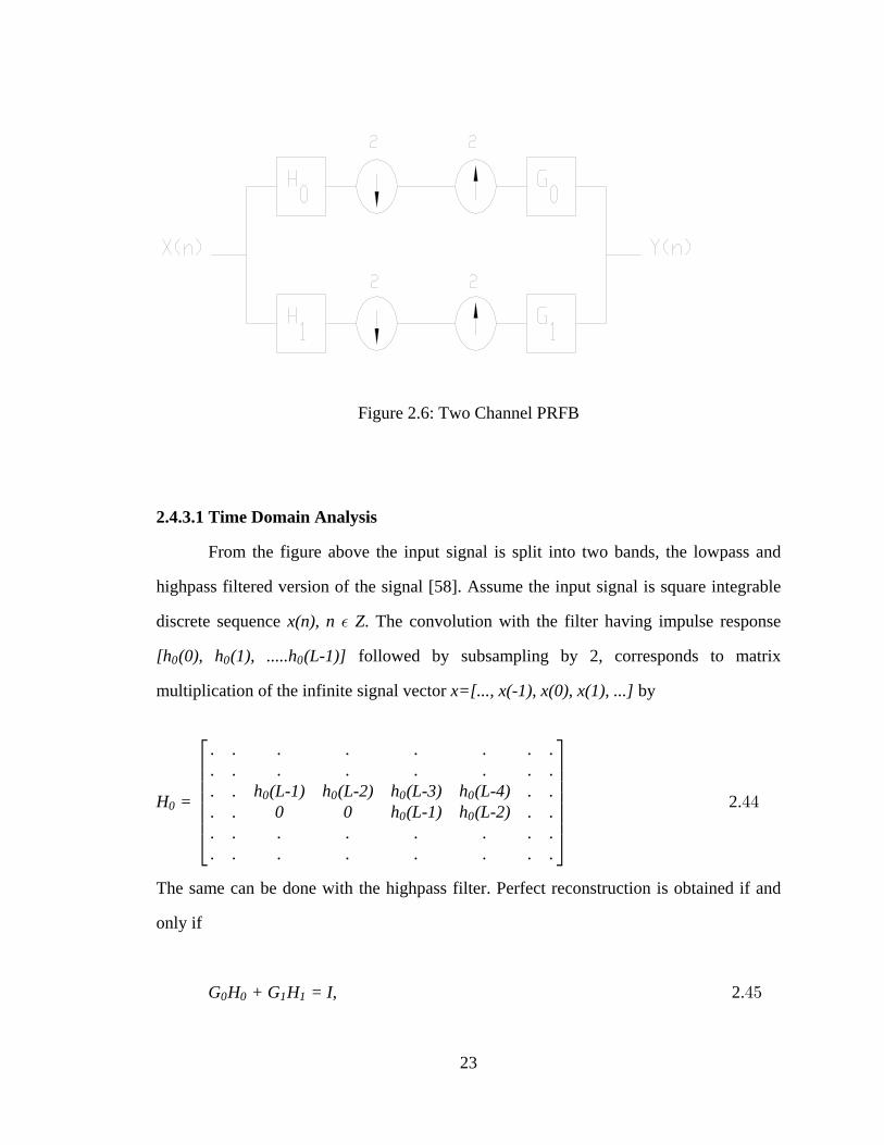
Figure 2.6: Two Channel PRFB

2.4.3.1 Time Domain Analysis

From the figure above the input signal is split into two bands, the lowpass and

highpass filtered version of the signal [58]. Assume the input signal is square integrable

discrete sequence . The convolution with the filter having impulse responsex(n), n Z%

[h (0), h (1), .....h (L-1)]0 0 0 followed by subsampling by 2, corresponds to matrix

multiplication of the infinite signal vector byx=[..., x(-1), x(0), x(1), ...]

H =

. . . . . . . .

. . . . . . . .

. . h (L-1) h (L-2) h (L-3) h (L-4) . .

. . 0 0 h (L-1) h (L-2) . .

. . . . . . . .

. . . . . . . .

00 0 0 0

0 0

Ô ×Ö ÙÖ ÙÖ ÙÖ ÙÖ ÙÖ ÙÕ Ø

2.%%

The same can be done with the highpass filter. Perfect reconstruction is obtained if and

only if

, 2.G H + G H = I0 0 1 1 %&

24

and if the orthogonality constraint, namely and is satisfied, thenG = H G = H0 10 1* *

2.4H H + H H = I.0 1* *

0 1 '

The orthogonality feature makes the synthesis filter the same as the analysis filter within

time reversal.

2.4.3.2 Polyphase Domain Analysis

Another way of looking at the system is to decompose both the signals and the

filters into polyphase components

2.4h(n) = h(Nn + 1). (

The polyphase components for the above case are just the even and odd subsequences of

filters and signals. Thus the lowpass filter can be decomposed into the following

, 2.4H (z) = H (z ) + z H (z )0 01 022 -1 2 )

where is the th polyphase component of the filter and is given byH i H0i 0

. 2.4H (z) = h (2n+i)z0i 0n

-n *

Similarly the input signal is decomposed into two sequences, but in reverse fashion

accounting for the shift-reversal when convolving the two components,

25

2.X(z) = X (z ) + zX (z )0 12 2 &!

X = X(2n-i)z .in

-n

The output of the system in terms of the polyphase decomposition is

2.5Y(z) = G (z )H (z )x (z ),c d" D p p p2 2 2 "

where and are matrices containing the polyphase components of the analysis andG Hp p

synthesis filters respectively, and contains the polyphase components of the inputxp

signal. The vector and are called the inverse and forward polyphase(1 z) (1 z )-1

transforms. Perfect reconstruction is possible if and only if

2.G (z)H (z) = I.p p &#

The matrix is called the transfer polyphase matrix. Aliasing isT = G Hp p p

canceled if is pseudo-circulant matrix and perfect reconstruction if and only if is aT Tp p

pseudo-circulant delay. In case of FIR filter perfect reconstruction is possible if and only

if the determinant of the analysis polyphase matrix is a delay. And if orthogonality is

assumed, then the condition for perfect reconstruction is

2.H (z)H (z) = I,s p p &$

where denotes transposition of the matrix, conjugation of the coefficients andHs

substitution of by .z z-1

26

2.4.3.3 Modulation Domain Analysis

The system can also be analyzed by directly finding the -domain expressions forz

all the signals. The output will then be

. 2.Y(z) = (G (z) G (z)) H (z) H (-z) X(z)H (z) H (-z) X(-z)

"# 0 1

0 0

1 1” •Œ &%

The solution to the above equation gives cancellation of aliasing. One such solution is

QMF (quadrature mirror filter) [81].

H (z) = H(z) G (z) = H(z)0 0

2.H (z) = H(-z) G (z) = -H(-z)1 1 &&

Y(z) = [X(z) X(-z)] H (z)H (z)-H (-z)H (-z)0

"# ” •0 0 0 0

The conditions for perfect reconstruction then becomes

2.5H (z) - H (-z) = 20 02 2 '

2.5 UNIFIED APPROACH

In this section, I will demonstrate the interconnection between the wavelets,

multiresolution analysis, and multirate filter banks discussed in the previous section.

These interconnections between the three concepts have created new venues for the

enhancement and elaboration of each of the particular concepts. Applications in one area

have simulated theoretical development in another area. Of particular significance to this

dissertation is the development of wavelet bases through the iteration of filter banks.

27

Most of the work in this area was first developed by S.Mallat and Y. Meyer [51], [52],

[56] and later extended by I. Daubechies, M. Veterlli and others [12], [13], [16], [21],

[65], [66].

2.5.1 WAVELET & MRA

The construction of wavelets from multiresolution analysis consists of a ladder of

spaces and a special function . In what follows the construction of{V }, j Z Vj 0% F %

wavelets from multiresolution analysis is outlined.

If we define such thatW , j Zj %

1. is the orthogonal complement of in i.e.W V Vj j j-"

2.5V = V Wj- j j " 9 (

and

2. .W W , if j kj k¼ Á

Then can be decomposed into mutually orthogonal subspaces and L (R) W#j

inherits the scaling property of .Vj

2.58 L (R) = W .j Z

# 9%

j

As with , there exits a vector such that its integer translates span , i.e.V W0 0G

. 2.5W =span{ }0 0nG *

Once the existence of is shown it remains to construct this function. The " two-G

scale relation " of the scaling and wavelet functions is used.

1. First a function with , an orthonormal basis for is determined.F F0n 0V

28

Because

there exists such thatF% V V h" "§ - n

2.F F(x) = h (2x-n).n

n '!

2. By definition

G F(x) = (-1) C (2x+n)n

nn-1

= 2. g (2x+n).n

nF '"

The above shows the construction of wavelets from multiresolution analysis

consisting of and a special function .{V }, j Z Vj 0% F %

The converse can also be proved for a space of band-limited functions and an

appropriately defined scaling function . Consider the following example where is aF V-"

space of band limited functions with frequencies defined in the interval and the[- , ]1 1

scaling function as . Then and its integer translates form orthonormalF F Fsinc(t) (t-k)

basis for . Similarly if is the space of band-limited functions with frequencies in theV V- 0"

interval , then and its integer translates constitute the orthonormal[- , ] (1/ 2) (t/2)1 12 2

È F

basis for . is a subspace of . And if is the space of functions band limited toV V V W0 0 - 0"

[- ,- ] [ , ] V V V1 11 12 2 0 - j∪ , then it is the orthogonal complement to in . In general if is the"

space of band-limited functions with frequencies in the interval and by(-2 , 2 )-j+1 -j+11 1

scaling the following relation is obtained,

V V , j Zj j-§ " %

, 2.V = V W j Zj-1 j j9 % '#

where is the space of band-limited functions withW , j Zj %

frequencies in the interval .(-2 ,2 ) (2 ,2 )-j+1 -j -j -j+11 1 1 1∪

29

And using the monotone sequential continuity theorem [67] the other properties

of the multiresolution analysis are satisfied.

2.5.2 FILTER BANK & MRA

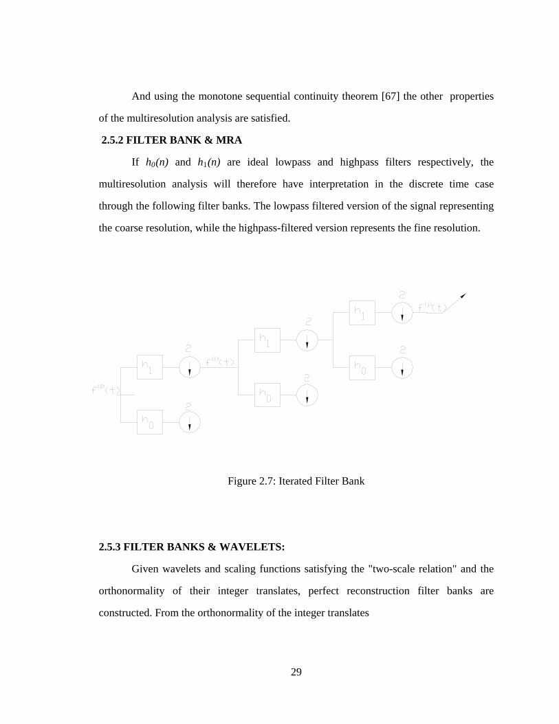
If and are ideal lowpass and highpass filters respectively, theh (n) h (n)0 "

multiresolution analysis will therefore have interpretation in the discrete time case

through the following filter banks. The lowpass filtered version of the signal representing

the coarse resolution, while the highpass-filtered version represents the fine resolution.

Figure 2.7: Iterated Filter Bank

2.5.3 FILTER BANKS & WAVELETS:

Given wavelets and scaling functions satisfying the "two-scale relation" and the

orthonormality of their integer translates, perfect reconstruction filter banks are

constructed. From the orthonormality of the integer translates

30

2. 9 9 $(t), (t-k) = . k '$

where $5 œ" 5 œ !! 5 Á !œ

Substituting for the scaling function using the "two-scale relation"

2. h (n),h (n-2k) = .0 0 k$ '%

Defining as a matrix with rows the above relation can be written asH h (n), h (n-2)...,0 0 0

2.H H =I0 0* '&

H H =I." "*

As shown above the compactly supported wavelets basis lead to the construction

of PRFB.

However, the converse is not always true. In figure 2.7 above the upper branch is

an infinite cascade of filters followed by subsampling by 2. The equivalent filter for a

cascade of blocks is given as j

2.6H (Z) = H(Z )(j) j

j=0

j-1# # '

followed by sampling by . As increases the length of increases to infinity. Instead2 j Hj (j)

we will consider the piecewise continuous function, , from the discrete iteratedf (x)(j)

filter i.e.

2.6f = 2 h (n) t .(j) (j) n n+12 2

12 j jŸ (

31

The fundamental question is to find out whether and to what function f (t)(j)

converges as given as an indicator function over the unit interval [0,1). Thej f (t)Ä ∞ (0)

limiting behavior depends on the nature of the filters. In order to construct wavelets of

compact support the filters must exhibit certain regularity condition. Under this regularity

condition the iterated function converges to a continuous function . The waveletF(t)

function is then obtained using the two-scale relation.

2.6 SUMMARY

In this chapter the basic concepts of wavelet analysis, multiresolution analysis and

multirate filter banks has been outlined. The historical development of wavelet analysis

from Fourier analysis as a result of the limitations of the latter has been discussed.

Several methods of analysis of perfect reconstruction filter banks has been discussed

using the two channel case as an example. Finally the essential connections between the

three concepts and their convergence to a single theory is shown. Basically, the

fundamental concepts essential to the understanding of the subsequent chapters are laid

down. The next chapter will deal the extension of these concepts to multiple dimensions.

32

CHAPTER 3

MULTIDIMENSIONAL EXTENSION

3.1 INTRODUCTION

Previous sections have been restricted to one-dimensional concepts. In the

following sections, I will extend these concepts to more than one dimension. The ultimate

objective of these extensions is to build multidimensional wavelets which are the topic of

the subsequent chapters. Most of the materials in this section are based on the results of

studies by Allenbach, Kovacevic, Vetterli , Lin, et al. (see [87], [38], [39], [84], [85]). In

the first section the background material such as multidimensional sampling and

multirate filter banks is outlined and latter the general multidimensional concepts are

discussed. At each stage of the development of the concepts, typical two- and three-

dimensional examples are constructed for illustration. All notations and definitions

applicable to this section such as multidimensional -transform and sampling arez

included in Appendix C.

3.2 PRELIMINARIES

Unlike the one-dimensional case, the multidimensional multirate signal

processing is completely based on a new set of concepts such as lattice, coset vectors and

so on [87]. In this section a brief introduction of these fundamental concepts is made.

3.2.1 Multidimensional Sampling

33

In single dimensional uniform sampling of signals, the sampling period or itsT

reciprocal the sampling density (sampling rate ) completely define the process. Unlike1/T

the one-dimensional case, multidimensional sampling is represented by an integer lattice

A defined as the set of all linear combinations of basis vectors withn n = [n ,n ,.....n ]1 2 nt

integer coefficients. The sampling sublattice is generated by the sampling matrix AD D

and is the set of integer vectors for some integer vector The proper definitionm n n= D .

of a sublattice requires a nonsingular sampling matrix with integer-valued entries.

Isotropic transformations in addition require the sampling matrices to have equal singular

value decomposition [47],[86]. A given sublattice can be generated by a number of

sampling matrices, each of which is related by a linear transformation represented by

unimodular integer matrix.

Figure 3.1: Multidimensional Sampling Lattice

34

The sampling lattice can be separable or nonseparable depending on whether the

sampling matrix is diagonal or not. The simplest form of sampling is the orthogonal

sampling generated by diagonal matrix. It appears when the sampling is done along each

dimension separately.

The unit cell is the set of points such that the disjoint union of its copies shifted to

all of the lattice points gives the input lattice. The number of input lattice samples

contained in the unit cell represents the reciprocal of the sampling density and is given by

N=det(D). The fundamental parallelepiped formed by basis vectors is an important unitn

cell. The Voronoi cell is another unit cell whose points are closer to the origin than any

other lattice points as shown in Figure 3.2 below.

Figure 3.2: Multidimensional Sampling Lattice and Cosets

Each point in a unit cell constitutes a vector and these vectors are called coset

vectors associated with . There are such vectors with defined as aD N { }k ,k ,...k k0 1 N-1 0

35

zero vector. A coset of a sublattice is the set of points obtained by shifting the entire

sublattice by an integer shift vectors . There are exactly distinct cosets and theirkl N

union gives the input lattice . A

Another important concept is the unit cell in the frequency domain. If a signal to

be sampled is band limited to the unit cell, no overlapping of spectra will occur and the

signal can be reconstructed from its samples. The reciprocal or modulation lattice is

actually the Fourier transform of the original lattice and its points represent the points of

replicated spectra in the frequency domain.

In general, the relation between the sampling matrix and the modulation or

reciprocal matrix is defined by

D 3.1s = 2 ( D ).1 -t

The columns of and represent the reciprocal and sampling vectors respectively.D Ds

3.2.1.1 DOWN SAMPLING AND DECIMATION:

A downsampler shown below samples an input signal by mapping points onx( )n

the sublattice to and discarding the rest.(See detail in [15], [87])A AD

36

Figure 3.3: Multidimensional Sampling Downsampler

The time, Fourier, and -domain expressions for the output of a downsampler arez

given by

3.2y( ) = x(D )n n

3.3Y( ) = X(D -2 D )s = =1N

U

-t -t

k % ct

1 k

3.4Y( ) = X(W (2 ) ) z k z1N

UD

D

k % ct

-1-1

1 ‰

37

where is n-dimensional real vector, is n-dimensional complex= z

vector and are n-dimensional integer vectors.n, k

From the Fourier expression, we see that the output at each frequency is formed=

by summing the input at a set of aliasing frequenciesN

D -2 D U-t -tc= 1 %k, k t . 3.5

All but one of these aliasing components have to be zero for alias cancellation.

Assume to be the set of frequencies in the admissible passband, then 3 3p, p=1 ... N-1ß ß

are sets obtained by shifting by the aliasing offsets ,3 1 2 D-tpk

. 3.63 1 3p p-t = { : + 2 D }= = k −

The frequency domain effect of downsampling can be interpreted as a mapping of

the baseband frequency region and the other identically shaped frequency regions( ) N-13

( , p=1 .. N-1) H( )3p ß Þß to the unit frequency cell. The process of prefiltering with a filter =

is to remove all but one of the above frequency regions. The downsampler with the filter

forms the decimator and the shape of the decimator filter has to be selected. Generally

there are many admissible passbands for a given downsampling matrix . TheD

fundamental property of an admissible passband is defined by the relation

3.73 3 F∩ p= p=1,...,N-1.

The intersection of and any of 's must be empty for an admissible passband. If two3 3p

frequencies that are separated by an aliasing offset are both in the passband is3

38

inadmissible. Hence, a passband is inadmissible if there exists , in and some3 = =1 2 3

integer vector such thatm

3.8= =1 2 p-t+ = 2 D + 2 k m1 1 .

Regardless of its shape, an admissible passband can have a hypervolume no larger

than of the size of unit frequency cell. However, with maximum hypervolume1/N

passbands, there exist frequencies at the boundary surfaces of the passbands that alias

onto their own negatives. These frequencies are called self-aliasing frequencies and are

defined as ( = =2 )= = =1 2 sa

3.9=sa l-t = D + 1 1k m.

There are more than one self-aliasing frequencies for each corresponding to differentkp

values of . These self-aliasing frequencies are useful to characterize the admissiblem

passbands. Actually the self-aliasing frequencies are essential in defining the boundaries

of the passband with maximum possible hypervolume. If a filter with the given passband

has real coefficients then must be symmetric about and the existence of these3 = = 0

self-aliasing frequencies is guaranteed. These concepts are illustrated using two examples

in subsequent sections.

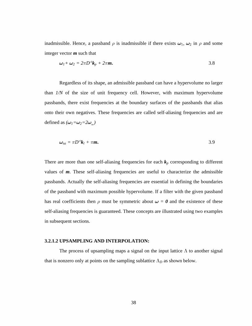
3.2.1.2 UPSAMPLING AND INTERPOLATION:

The process of upsampling maps a signal on the input lattice to another signalA

that is nonzero only at points on the sampling sublattice as shown below.AD

39

Figure 3.4: Multidimensional Sampling Upsampler

The time, frequency and expressions of the output of the upsamplerz-transform

are given by

3.10y( ) = x(D ) if D if D

n n nnœ -1 -1

-1% A

A! Â ß

3.11Y( ) = X(D )= =t ß

40

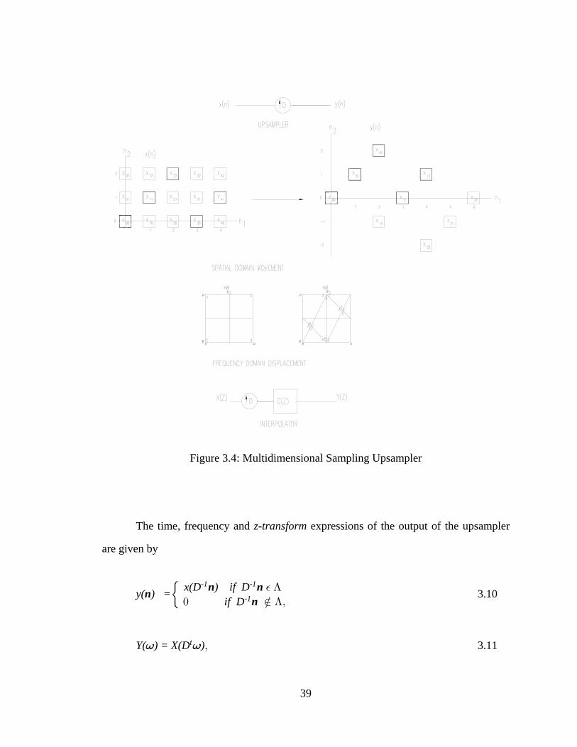
3.12Y( ) = X( ) z zD Þ

The output of the upsampler in the frequency domain results in the reduction of

the passband and the skewing of their orientation.

Figure 3.5: Frequency Domain Baseband Change

As a result images of the unit cell are mapped to regions surrounding the

baseband resulting in complete images of one period of in . It is thereforeN X( ) Y( )= =

essential for an upsampler to be followed by a filter that stops all but one of theG( )=

images. An interpolator is the combination of the upsampler followed by such a filter.

3.2.2 POLYPHASE DECOMPOSITION

The polyphase decomposition of a signal is an important tool in multirate signal

processing. If are the set of coset vectors associated with the samplingk k k1 2 N-1, ,...,

matrix , then the th polyphase component of of the signal is formed byD p x ( ) x( )p n n

shifting by and downsampling the result:x( ) -n kp

41

3.13x ( ) = x(D + )p pn n k Þ

A signal can be recovered from its polyphase components by

3.14X( ) = x(D + ) z n k zk

k

-

% A

Þ

3.2.3 EXAMPLES

The following two typical examples used by M. Veterlli and J. Kovacevic are

used to illustrate the above concepts [41]. These 2- and 3- examples are also used inD D

subsequent sections.

Example 1: Two-dimensional sampling

Two-dimensional quincunx sampling is generally represented by

. 3.15A % mQ 1 2 1 2 it = {(n + n ) n + n = 2k, n , k }l

Let us consider the following specific quincunx sampling matrix given by

3.16D= 1 1-1 1” •

The determinant of being equal to 2 there are 2 distinct coset vectors defined belowD tpk

3.17k k0 1= , =0 10 0” • ” •

42

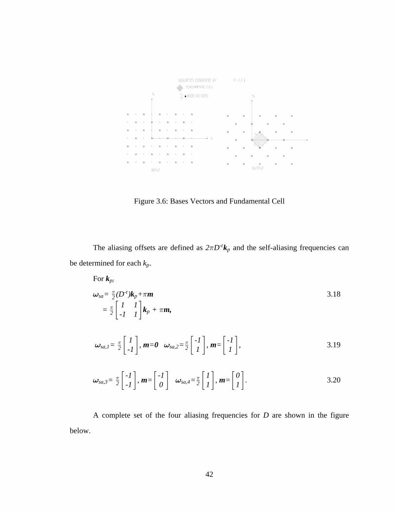
Figure 3.6: Bases Vectors and Fundamental Cell

The aliasing offsets are defined as and the self-aliasing frequencies can2 D1 -tpk

be determined for each .kp

For kp:

3.18=sa p2-t= (D ) +1 k m1

= 12 p” •1 1-1 1 + k m,1

, 3.19= =sa,1 sa,22 2= , = = , =1 -1 -1-1 1 1

1 1” • ” • ” •m 0 m

. 3.20= =sa,3 sa,42 2= , = = , =-1 -1 1 0-1 0 1 1

1 1” • ” • ” • ” • m m

A complete set of the four aliasing frequencies for are shown in the figureD

below.

43

Figure 3.7: Example of Aliasing Frequencies for D

A number of admissible passbands for decimation filters with real impulse

responses can be drawn using these frequencies. These self-aliasing frequencies define

the boundaries of the passbands with maximum possible hypervolume of . It is1N

D(2 )1

possible to use horizontal, vertical, bandpass filters for the sampling matrix as shown in

Figure 3.8 below.

44

Figure 3.8: Admissible Passbands Generated by D

Example 2: Three dimensional sampling

The face centered orthogonal (FCO) sampling lattice is described by [31]

. 3.21A % mQ 1 2 3 1 2 3 it = {(n + n + n ) n + n + n = 2k, n , k }l

Let us consider the following specific sampling matrix

. 3.22D=1 1 01 0 10 1 1

Ô ×Õ Ø

45

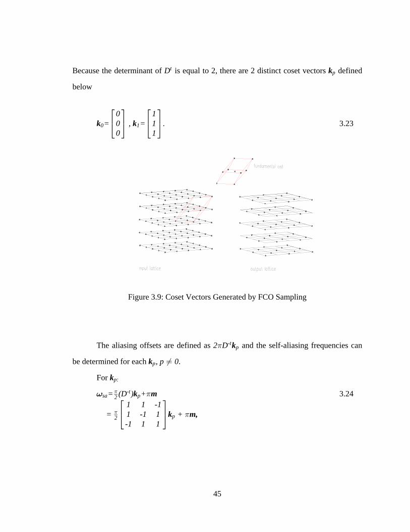
Because the determinant of is equal to 2, there are 2 distinct coset vectors definedDtpk

below

. 3.23k k0 1= , =0 10 10 1

Ô × Ô ×Õ Ø Õ Ø

Figure 3.9: Coset Vectors Generated by FCO Sampling

The aliasing offsets are defined as and the self-aliasing frequencies can2 D1 -tpk

be determined for each .kp, p 0Á

For kp:

3.24=sa p2-t= (D ) +1 k m1

= 12 pÔ ×Õ Ø

1 1 -11 -1 1-1 1 1

+ k m,1

46

,= =sa,1 sa,22 2= , = = , =1 -1 -11 -1 -11 -1 -1

1 1Ô × Ô × Ô ×Õ Ø Õ Ø Õ Ø m 0 m

,= =sa,3 sa,42 2= , = , = , =-1 -1 -1 -11 0 -1 -11 0 1 0

1 1Ô × Ô × Ô × Ô ×Õ Ø Õ Ø Õ Ø Õ Øm m

,= =sa,5 sa,62 2= , = = , =1 0 1 0-1 -1 -1 -11 0 -1 -1

1 1Ô × Ô × Ô × Ô ×Õ Ø Õ Ø Õ Ø Õ Øm m

.= =sa,7 sa,82 2= , = = , =1 0 -1 -11 0 1 0-1 -1 -1 -1

1 1Ô × Ô × Ô × Ô ×Õ Ø Õ Ø Õ Ø Õ Øm m

The complete set of the eight aliasing frequencies for that lie on the boundaryD

of any maximum-volume passband are shown below.

Figure 3.10: Baseband and Aliasing Frequency FCO Sampling

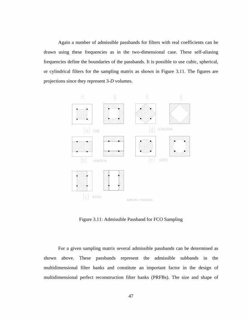
47

Again a number of admissible passbands for filters with real coefficients can be

drawn using these frequencies as in the two-dimensional case. These self-aliasing

frequencies define the boundaries of the passbands. It is possible to use cubic, spherical,

or cylindrical filters for the sampling matrix as shown in Figure 3.11. The figures are

projections since they represent 3- volumes.D

Figure 3.11: Admissible Passband for FCO Sampling

For a given sampling matrix several admissible passbands can be determined as

shown above. These passbands represent the admissible subbands in the

multidimensional filter banks and constitute an important factor in the design of

multidimensional perfect reconstruction filter banks (PRFBs). The size and shape of

48

these subbands that are determined by the sampling matrix D determine the number of

channels and design of filters in PRFBs. Hence, a choice of any particular passband has

to be carefully selected based on alias cancellation and other filter design considerations,

including conditions for perfect reconstruction. In what follows the conditions for perfect

reconstruction are discussed.

3.3 MULTIDIMENSIONAL FILTER BANKS

One-dimensional filter banks have been extensively studied and several design

methods have been successfully developed. Recently there has been a lot of interest in

filter banks in multiple dimensions. However, the extension of filter banks into multiple

dimensions is still an area of extensive research. Here I will briefly review some of the

important concepts and results of recent research in multidimensional filter banks. (See

details in [87], [78], [91], [13], [41]). The multirate filter bank can be considered as a

hierarchy with sampling and filtering constituting the basic operations at the lowest level.

A multidimensional -channel filter bank is shown below. The discussion isN

restricted to uniform band, maximally sampled filter banks in which there are N=det(D)

channels with the same sampling matrix .D

49

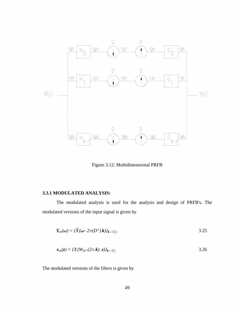
Figure 3.12: Multidimensional PRFB

3.3.1 MODULATED ANALYSIS:

The modulated analysis is used for the analysis and design of PRFB's. The

modulated versions of the input signal is given by

, 3.25xsm U-t( ) = {X ( - 2 (D ). )}= =s 1 k k % c

t

3.26x z k zm U .D( ) = {X (W (2 . ). )}-1ct1 k %

The modulated versions of the filters is given by

50

, 3.27H ( ) = {H ( - 2 (D ). )} U , i {0, 1, .....N-1}s sm i , -t t

c= = 1 % %k k

. 3.28H ( ) = {H (W (2 . ). )}, U , i {0, 1, .....N-1}m i D ctz k z k-1 1 % %

The output of the system after upsampling and filtering in the synthesis bank is given by

, 3.29Y ( ) = (G ( ).G ( )...G ( )).H ( ).x ( )s ss s s s= = = = = =1N 0 1 N-1 m m

, 3.30Y ( ) = (G ( ).G ( )...G ( )).H ( ).x ( )z z z z z z1N 0 1 N-1 m m

, 3.31Y ( ) = (G ( ).G ( )...G ( )).H ( )X( )z z z z z z1N 0 1 N-1 AC

where the th element of is .(m,p) H ( ) H (W (2 ) )AC m pDz k z-1 1

The filter bank output is identical to the input if and only if

3.32 Ô × Ô ×Õ Ø Õ Ø

G ( )

G ( )= NH ( )

0

N-1AC-1

z

zzã ã

"

!

To achieve perfect reconstruction it is necessary and sufficient that the analysis

component (AC) matrix be invertible and the vector of synthesis filters be chosen as the

first column of . However, the design of such a filter bank is not easy as it is oftenH ( )AC-1 z

difficult to invert an arbitrary AC matrix. Besides, it may result in higher order analysis

filters and there is no simple way to ensure the stability of the synthesis filters. The

analysis and design of PRFB's is easily done using the polyphase form.

51

3.3.2 POLYPHASE ANALYSIS:

The polyphase approach was introduced for the analysis and design of one-

dimensional PRFB's. A convenient way of alias cancellation in multidimensional system

is to decompose both signals and filters into polyphase components each corresponding

to one of the cosets of the output lattice. The polyphase decomposition of the input signal

is given by

3.33X( ) = X ( ) = x ( )z z z p zk

kk

% U

- D t Di p

ct

and

3.34X ( ) = x(D - ).kn

nz n k z% m

-n

where is the vector of the inverse polyphase transform ( ) = { }p z zi Uk

k % ct

and is the vector containing the polyphase components of the input signal ( )x zp

3.35 ( ) = {X ( )} .x z zp Uk k % ct

Similarly, the polyphase components of the filter could be defined asH(z)

3.36H( ) = H ( ) = h ( ),z z z p zk

kk

% U

- D t Di p

ct

and

, 3.37H ( ) = h(D - ).kn

nz n k z% m

-n

where is the vector of the forward polyphase transform and p z z zf U p-( ) = { } h ( )k

k % ct

= {H ( )}k kz U% ct is the vector containing the polyphase components of the filter.

Thus a single-input linear shift-variant system can be expressed as a multi-input

shift-invariant system. To obtain the polyphase expansion first we have to select {k ,0

k ...k1 N-1} D, the coset vectors associated with the sampling matrix . Then we have to

determine the polyphase components of the input signal and each of the analysis filter in

52

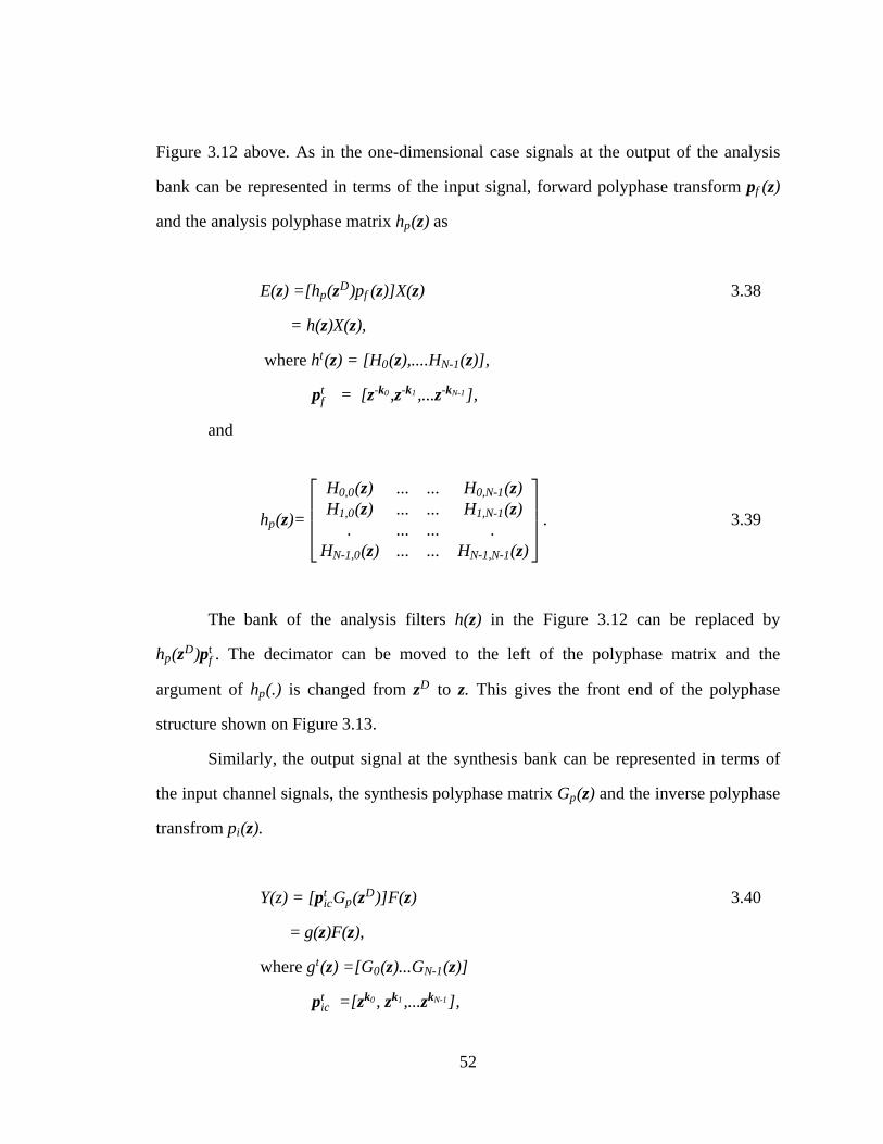
Figure 3.12 above. As in the one-dimensional case signals at the output of the analysis

bank can be represented in terms of the input signal, forward polyphase transform p zf ( )

and the analysis polyphase matrix ash ( )p z

3.38E( ) =[h ( )p ( )]X( )z z z zp fD

= h( )X( ),z z

where h ( ) = [H ( ),....H ( )],t0 N-1z z z

= [ , ,... ],p z z zft - - -k k k0 1 N-1

and

. 3.39h ( )=

H ( ) ... ... H ( )H ( ) ... ... H ( )

. ... ... .H ( ) ... ... H ( )

p

0,0 0,N-1

1,0 1,N-1

N-1,0 N-1,N-1

z

z zz z

z z

Ô ×Ö ÙÖ ÙÕ Ø

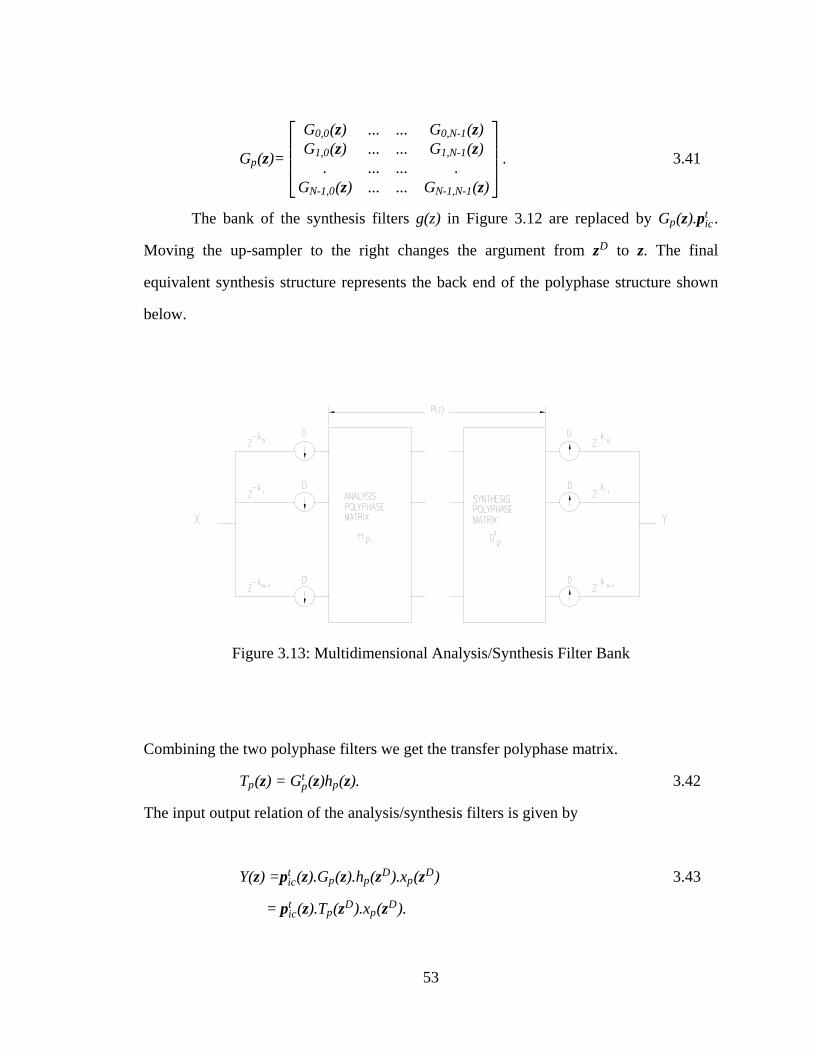
The bank of the analysis filters in the Figure 3.12 can be replaced byh( )z

h ( )pD

fz pt . The decimator can be moved to the left of the polyphase matrix and the

argument of is changed from to This gives the front end of the polyphaseh (.) .pDz z

structure shown on Figure 3.13.

Similarly, the output signal at the synthesis bank can be represented in terms of

the input channel signals, the synthesis polyphase matrix and the inverse polyphaseG ( )p z

transfrom p ( ).i z

3.40Y(z) = [ G ( )]F( ) p z zict D

p

= g( )F( ),z z

where g ( ) =[G ( )...G ( )]t0 N-1z z z

p z z zict =[ , ,... ],k k k0 1 N-1

53

. 3.41G ( )=

G ( ) ... ... G ( )G ( ) ... ... G ( )

. ... ... .G ( ) ... ... G ( )

p

0,0 0,N-1

1,0 1,N-1

N-1,0 N-1,N-1

z

z zz z

z z

Ô ×Ö ÙÖ ÙÕ Ø

The bank of the synthesis filters in Figure 3.12 are replaced by .g(z) G ( ).p ictz p

Moving the up-sampler to the right changes the argument from to . The finalz zD

equivalent synthesis structure represents the back end of the polyphase structure shown

below.

Figure 3.13: Multidimensional Analysis/Synthesis Filter Bank

Combining the two polyphase filters we get the transfer polyphase matrix.

3.42T ( ) = G ( )h ( ).p pptz z z

The input output relation of the analysis/synthesis filters is given by

3.43Y( ) = ( ).G ( ).h ( ).x ( )z p z z z zict D D

p p p

= p z z zict D D

p p( ).T ( ).x ( ).

54

The following set of conditions are set based on the above input/output relations (See

[40]):

1. Aliasing is cancelled if and only if the inverse polyphase transform vector is the leftpi

eigenvector of the transfer polyphase matrix in the upsampled domain that isT ( )pDz

3.44p z z pi it D t

p.T ( ) = T( ). ,

T(z) T (z ) the eigenvalue of is a scalar polynomial and defines the overall transferpD

function of the filter bank. If we let denote the vector that makes causal, thenzkc ic

N-1% U pt t

3.45Y( ) = .T ( ).x ( ),z z p z zk t D Di p pN-1

and since we obtainX( ) = x ( )z p zit D

p

. 3.46Y( ) = T( ).X( )z z z zkN-1

Thus the output is a scalar multiple of the input.

2. Perfect reconstruction is achieved if and only if the eigenvalue associated with theT( )z

eigenvector in 1 is monomial i.e. pit

3.47T( ) = c. .z z-k

And since ,z z zk -k -N-1 = n

3.48Y( ) = c X( ).z z z-n

55

The output is a shifted version of the input.

3. Perfect reconstruction with FIR filters is achieved if and only if the determinant

of the analysis polyphase matrix is monomial i.e.

3.49det(h ( )) = .p-z z k

If we choose then is FIR if is FIR and becomes aG ( ) = adj(H ( )) G ( ) H ( ) Tp p p p pz z z z

diagonal matrix of delays,

3.50Y( ) = ( ).I.x ( )z z p z zkN-1it D

p

= X( ).z z-n

The two representations polyphase and modulated domain analysis are time-

frequency representation and are related by Fourier Transform.

3.3.3 ADDITIONAL CONSTRAINTS

Once perfect reconstruction is obtained some additional requirements can be

imposed on the filter banks. The most important ones are orthogonality and linear phase

[4], [5].

3.3.3.1 ORTHOGONAL CASE:

As was mentioned in the one-dimensional case, a matrix is paraunitary if it

satisfies

3.51H(z)H(z) =H(z)H(z) = c I.s s ‚

56

This matrix becomes orthogonal on the unit hypercircles . If the analysis(z = e , i=1..n)ij=i

polyphase matrix is orthogonal, then

3.52H (z)H (z) = I.p ps

By choosing the following matrix, a perfect reconstruction system is obtained.

3.53G (z) = z H (z).p p-k s

Suppose the modulation matrix defined above is orthogonal, thenH (z)m

3.54H ( - 2 (D ).k)= H (W (2 .k).z)H (W (2 .k).z) i i i-t

k UD Ds s= 1 1 1

% ct

-1 -1

= .N$ij

If as the first row of perfect reconstruction is achieved.(G (z)....G (z)) H (z)0 N-1 m

And if is real it is the z-transform of the cross correlation sequence H (z)H (z) r (n) =i j ijs

<h (k), h (k+n)>i j . This means that each filter is orthogonal to its translates with respect to

the lattice. Thus the set is an orthonormal set and is the{h ( +D ), i=0,...N-1, , }ink n k n % m

lattice extension of the orthogonality relations with respect to the shifts in the one-

dimensional case.

3.3.3.2 LINEAR PHASE:

If a real filter is linear phase, it can be written as

3.55H(z) = a.D(z).H(z),s

where a denotes symmetry and

57

3.56D(z) = z = z .-(P+Q)

i=1

n

i-(p +q )# i i

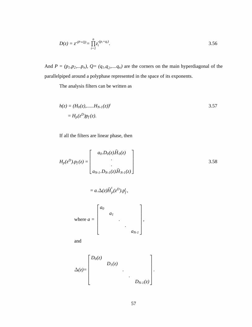
And are the corners on the main hyperdiagonal of theP = (p ,p ,...p ), Q= (q ,q ,....q )1 2 n 1 n2

parallelpiped around a polyphase represented in the space of its exponents.

The analysis filters can be written as

3.57h(z) = (H (z),......H (z))0 N-1t

= .H (z )p (z)p fD

If all the filters are linear phase, then

3.58H (z ).p (z) =

a .D (z).H (z)..

a .D (z).H (z)

p fD

0 0 0

N-1 N-1 N-1

Ô ×Ö ÙÖ ÙÕ Ø

s

s

= ,a. (z)H (z ).p? s pt D

ft

where , a =

aa

..

a

Ô ×Ö ÙÖ ÙÖ ÙÖ ÙÕ Ø

0

1

N-1

and

.?(z)=

D (z)D (z)

..

D (z)

Ô ×Ö ÙÖ ÙÖ ÙÖ ÙÕ Ø

0

1

N-1

58

The above can be either used to test linear phase of the filter banks or put a constraint in

the design of linear phase filters.

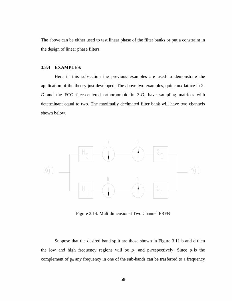
3.3.4 EXAMPLES:

Here in this subsection the previous examples are used to demonstrate the

application of the theory just developed. The above two examples, quincunx lattice in 2-

D D and the FCO face-centered orthorhombic in 3- , have sampling matrices with

determinant equal to two. The maximally decimated filter bank will have two channels

shown below.

Figure 3.14: Multidimensional Two Channel PRFB

Suppose that the desired band split are those shown in Figure 3.11 b and d then

the low and high frequency regions will be and p respectively. Since p is thep0 1 1

complement of p any frequency in one of the sub-bands can be trasferred to a frequency0

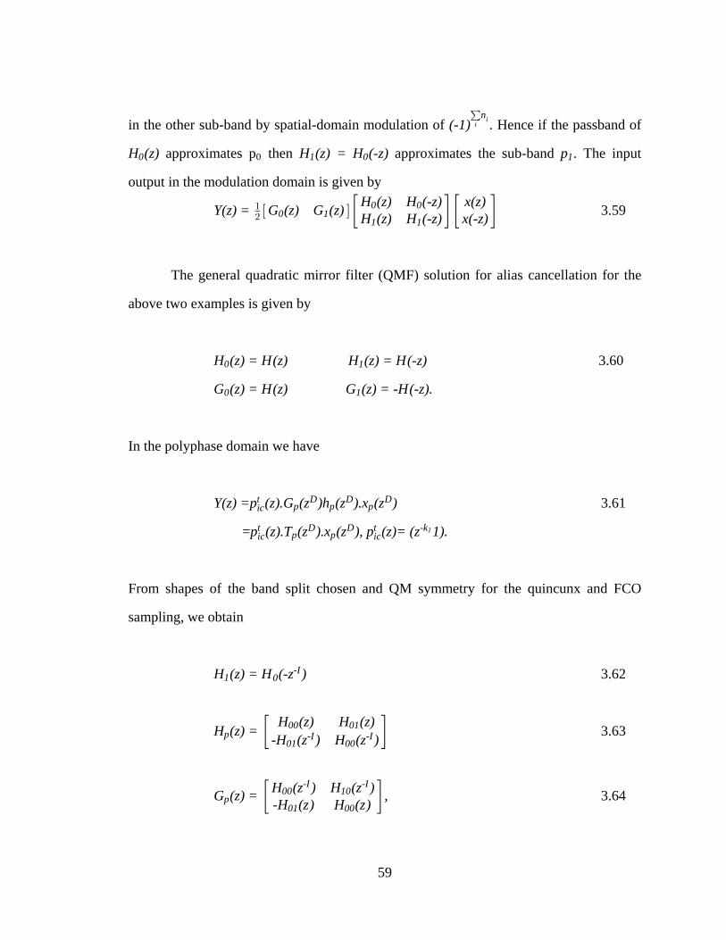
59

in the other sub-band by spatial-domain modulation of . Hence if the passband of(-1) iin

H (z) H (z) = H (-z) p0 1 0 1 approximates p then approximates the sub-band . The input0

output in the modulation domain is given by

3.59Y(z) = G (z) G (z) H (z) H (-z) x(z)H (z) H (-z) x(-z)

"# c d” •” •0 1

0 0

1 1

The general quadratic mirror filter (QMF) solution for alias cancellation for the

above two examples is given by

3.60H (z) = H(z) H (z) = H(-z)0 1

G (z) = H(z) G (z) = -H(-z).0 1

In the polyphase domain we have

3.61Y(z) =p (z).G (z )h (z ).x (z ) ict D D D

p p p

=p (z).T (z ).x (z ), p (z)= (z 1).ic ict D D t -k

p p 1

From shapes of the band split chosen and QM symmetry for the quincunx and FCO

sampling, we obtain

3.62H (z) = H (-z )1 0-I

3.63H (z) = H (z) H (z)-H (z ) H (z )p

00 01

01 00-I -I” •

, 3.64G (z) = H (z ) H (z )-H (z) H (z)p

00 10-I -I

01 00” •

60

and for perfect reconstruction (PR) FIR filter bank, the following has to be satisfied

, 3.65det(H (z)) = czpk1

which reduces to

. 3.66H (z)H (z ) + H (z)H (z ) = 100 00 01 01-I -I

For quincunx:

. 3.67H (z ,z )H (z ,z ) + H (z ,z )H (z ,z ) = 100 1 2 00 01 1 2 011 2 1 2-1 -1 -1 -1

For FCO:

3.68H (z ,z ,z )H (z ,z ,z ) + H (z ,z ,z )H (z ,z ,z ) = 100 1 2 3 00 01 1 2 3 011 2 3 1 2 3-1 -1 -1 -1 -1 -1

In addition to the prefect reconstruction requirement the following two additional

constraints may be considered in the general case.

1. Orthogonal:

If the analysis filter is paraunitary, then

3.69H (z) = H (z) H (z)

cz H (z ) -cz H (z )p00 01

-k -I -k -I01 00

” •1 1

H (z) H (z) (H (z) = -z H (-z)1 0 1 00-k is completely specified by , the two polyphase1 s

components are the same size and the polyphase components of H (z) have to satisfy the0

power complementary property above. This requirement automatically excludes the

desired diamond shaped passband because both filters have the same symmetry and size.

2. Linear Phase:

61

For the above examples the general linear phase testing conditions reduces to

3.70 H (z ) = H (z )1 1

z za D (z)

a D (z)p pD -D

1 1-k k

0 0

1 1Œ Œ Œ Œ1 1

where and represent the symmetry of and a a h h0 1 0 1

are monomials related to the size ofD (z ,z ), D (z , z )0 1 2 1 1 2

the filters.

For the two-channel real FIR case linear phase and orthogonality are mutually

exclusive.

3.4 SYNTHESIS OF MULTIDIMENSIONAL FILTER BANKS:

In the following sections, we look at design structures, which meet the perfect

reconstruction conditions derived above. One of the desirable properties for the analysis

and synthesis banks is that they should both consist of finite-impulse response filters thus

eliminating problems related to stability. Given an analysis filter that is FIR, then a

synthesis filter bank of perfect reconstruction system is FIR if and only if the determinant

of the polyphase matrix of the analysis filter bank is monomial in . There are twoz

fundamental approaches to satisfying the above perfect reconstruction conditions. One

possibility is to construct the analysis polyphase matrix so that its inverse mayh (z)p

readily be found. This approach is used for one dimensional PRFB's and needs to be

extended to multiple dimensions. The second possibility sees the polyphase matrix

equation not as that relating the analysis and synthesis filters, but as a set of scalar

equations relating the impulse response coefficients.

3.4.1 NUMERICAL OPTIMIZATION:

62

Numerical optimization is used to solve the set of scalar equations relating the

impulse response coefficients. Additional conditions such as FIR and equal size filters

are incorporated as a set of quadratic equality constraints. The constraints are nonlinear

and nonconvex and several standard nonlinearity constrained optimization methods are

used to design the filter banks. Symmetry is also used to reduce the number of variables

and independent constraints. However, due to the large numbers of variables and

constraints the optimization is often complex.

3.4.2 CASCADE:

The condition to achieve PR for FIR analysis and synthesis filters requires that

the det to be a shift. These shift vectors are factorizable and so is the determinant.(H (z))p

A polynomial matrix whose determinant is factorizable can itself be factorized. The

determinant of a product is a product of the determinants. Thus if is constructedH (z)p

from the cascade(product) of matrices which satisfy condition (3.48) then will alsoH (z)p

satisfy the same condition. Polynomial matrix factorization methods can be used to

design cascade structures for (see [21], [14], [16], [29]). Thus cascade structuresH (z)p

can be used to find set of filters so that meets the perfect reconstruction conditionH (z)p

stated above.

3.71H (z) = U D (z) U D (z)U p n n 1 1 0â

where are arbitrary constant coefficient matricesUi

are diagonal matrices of shifts.D (z)i

Cascade structures not only have very low complexity, but also have the

advantages of generating higher order filters from lower-order ones. Several approaches

63

are possible depending on which constraints have to be met. One can require the filter

bank to be paraunitary, linear phase, or both [73], [74].

3.4.2.1 ORTHOGONAL:

In the orthogonal case the cascade if formed by combining orthogonal building

blocks, i.e. orthogonal and diagonal delay matrices.

3.72H (z) = U U D (z)p 0 i ii=1

n# where are unitary matricesUi

are diagonal matrices of delays.D (z)i

For the two channel -dimensional case the real FIR orthogonal polyphase matrixn

Hp can be written as

. 3.73H (z) = H (z) H (z)

cz H (z) -cz H (z)p00 01

-k -k01 00

” •s

The following cascade will produce PR set containing two filters of the same size:

, 3.74H (z) = U U1 00 zp 0 ij

j=1i=1

k n

i-1

##Œ

where is unitary, i.e.Uij

.U = 1 -aa 1i1,2

i1,2

i1,2Œ

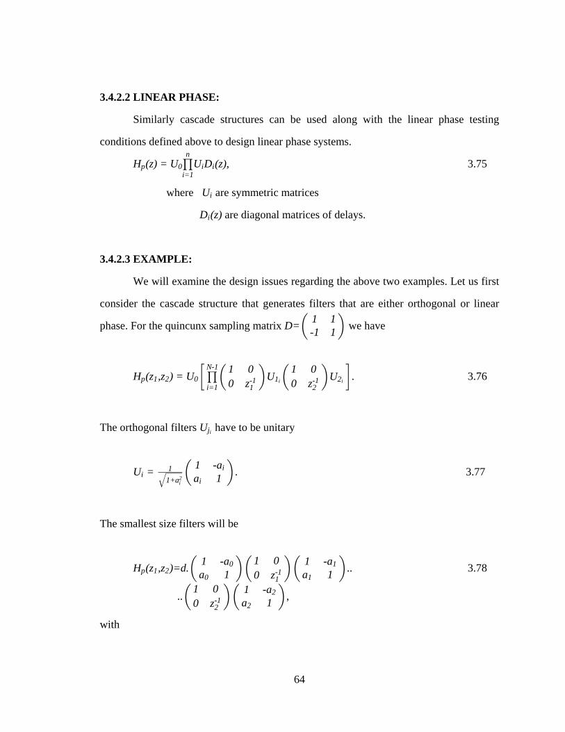
64

3.4.2.2 LINEAR PHASE:

Similarly cascade structures can be used along with the linear phase testing

conditions defined above to design linear phase systems.

, 3.75H (z) = U U D (z)p 0 i ii=1

n# where are symmetric matricesUi

are diagonal matrices of delays.D (z)i

3.4.2.3 EXAMPLE:

We will examine the design issues regarding the above two examples. Let us first

consider the cascade structure that generates filters that are either orthogonal or linear

phase. For the quincunx sampling matrix we haveD= 1 1-1 1Œ

. 3.76H (z ,z ) = U 1 0 1 00 z 0 zU Up 1 2 0

i=1

N-1

1 2-1 -11 2” •#Œ Œi i

The orthogonal filters have to be unitaryUji

. 3.77U = 1 -aa 1i

11+a

i

iÉ i2 Œ

The smallest size filters will be

3.78H (z ,z )=d. ..1 -a 1 -aa 1 a 1

1 00 zp 1 2

0 1

0 11-1Œ Œ Œ

, ..1 00 z

1 -aa 1Œ Œ

2-1

2

2

with

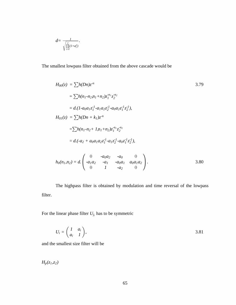
65

.d= 1

(1+a )Ë#i=0

2

i2

The smallest lowpass filter obtained from the above cascade would be

3.79H (z) = h(Dn)z 00-n

= h(n -n ,n +n )z z1 2 1 2 1 2-n -n1 2

= ,d.(1-a a z -a a z -a a z z )0 1 1 2 0 21 2 1 2-1 -1 -1 -1

H (z) = h(Dn + k )z01 1-n

= h(n -n + 1,n +n )z z1 2 1 2 1 2-n -n1 2

= ,d.(-a + a a a z -a z -a z z )2 0 1 2 1 01 2 1 2-1 -1 -1 -1

. 3.80h (n ,n ) = d.-a a -a

-a a -a -a a a a a1 -a

0 1 2

0 2 0

1 2 1 0 1 0 1 2

2

Î ÑÏ Ò

! !

! !

The highpass filter is obtained by modulation and time reversal of the lowpass

filter.

For the linear phase filter has to be symmetricUji

, 3.81U = 1 aa 1i

i

iŒ

and the smallest size filter will be

H (z ,z )p 1 2

66

= . 3.82Œ Œ Œ Œ Œ1 a 1 a 1 aa 1 a 1 a 1

1 0 1 00 z 0 z

0 1 2

0 1 21 2-1 -1

The lowpass filter obtained from the above cascade will be

3.83H (z) = h(Dn)z00-n

= h(n -n ,n +n )z z1 2 1 2 1 2-n -n1 2

= ,1+a a z +a a z +a a z z0 1 1 2 0 21 2 1 2-1 -1 -1 -1

H (z) = h(Dn + k )z01 1-n

= h(n -n + 1,n +n )z z1 2 1 2 1 2-n -n1 2

= ,a + a a a z +a z +a z z2 0 1 2 1 01 2 1 2-1 -1 -1 -1

3.84h (n ,n ) = a a a

a a a a a a a a1 a

0 1 2

0 2 0

1 2 1 0 1 0 1 2

2

Î ÑÏ Ò

! !

! !

= .Î ÑÏ Ò

! !

! !

a 1a a a a a a

1 a

2

1 2 1 1 1 2

2

For FCO sampling matrix , the cascade structures generates theD=1 1 01 0 10 1 1

Î ÑÏ Ò

following filters

H (z ,z ,z )p 1 2 3

= . 3.85U U1 0 1 00 z 0 zU U

1 00 z0 3

i=1

N-1

1 2-1 -11 2

3-1” •#Œ Œ Œi i i

Again for the orthogonal filters have to be unitaryU ji

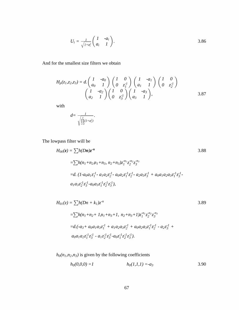
67

. 3.86U = 1 -aa 1i

11+a

i

iÉ i2 Œ

And for the smallest size filters we obtain

H (z ,z ,z ) = d. 1 -a 1 -aa 1 a 1

1 0 1 00 z 0 zp 1 2 3

0 1

0 11 2-1 -1Œ Œ Œ Œ

, 3.87Œ Œ Œ1 -a 1 -aa 1 a 1

1 00 z

2 3

2 33-1

with

.d= 1

(1+a )Ë#i=0

3

i2

The lowpass filter will be

3.88H ( ) = h(D )00-z n z n

= h(n +n ,n +n , n +n )z z z1 2 1 3 2 3 1 2 3-n -n -n1 2 3

=d. (1-a a z - a a z - a a z z - a a z + a a a a z z -0 1 1 2 0 2 2 3 0 1 2 31 2 1 2 3 1 3-1 -1 -1 -1 -1 -1 -1

,a a z z -a a z z z )1 3 0 32 3 1 2 3-1 -1 -1 -1 -1

3.89H (z) = h(Dn + k )z01 1-n

= h(n +n + 1,n +n +1, n +n +1)z z z1 2 1 3 2 3 1 2 3-n -n -n1 2 3

=d.(-a + a a a z + a a a z + a a a z z - a z +3 0 1 3 1 2 3 0 2 3 21 2 1 2 3-1 -1 -1 -1 -1

.a a a z z - a z z -a z z z )0 1 2 1 01 3 2 3 1 2 3-1 -1 -1 -1 -1 -1 -1

is given by the following coefficientsh (n ,n ,n )0 1 2 3

3.90h (0,0,0) =1 h (1,1,1) =-a 0 0 3

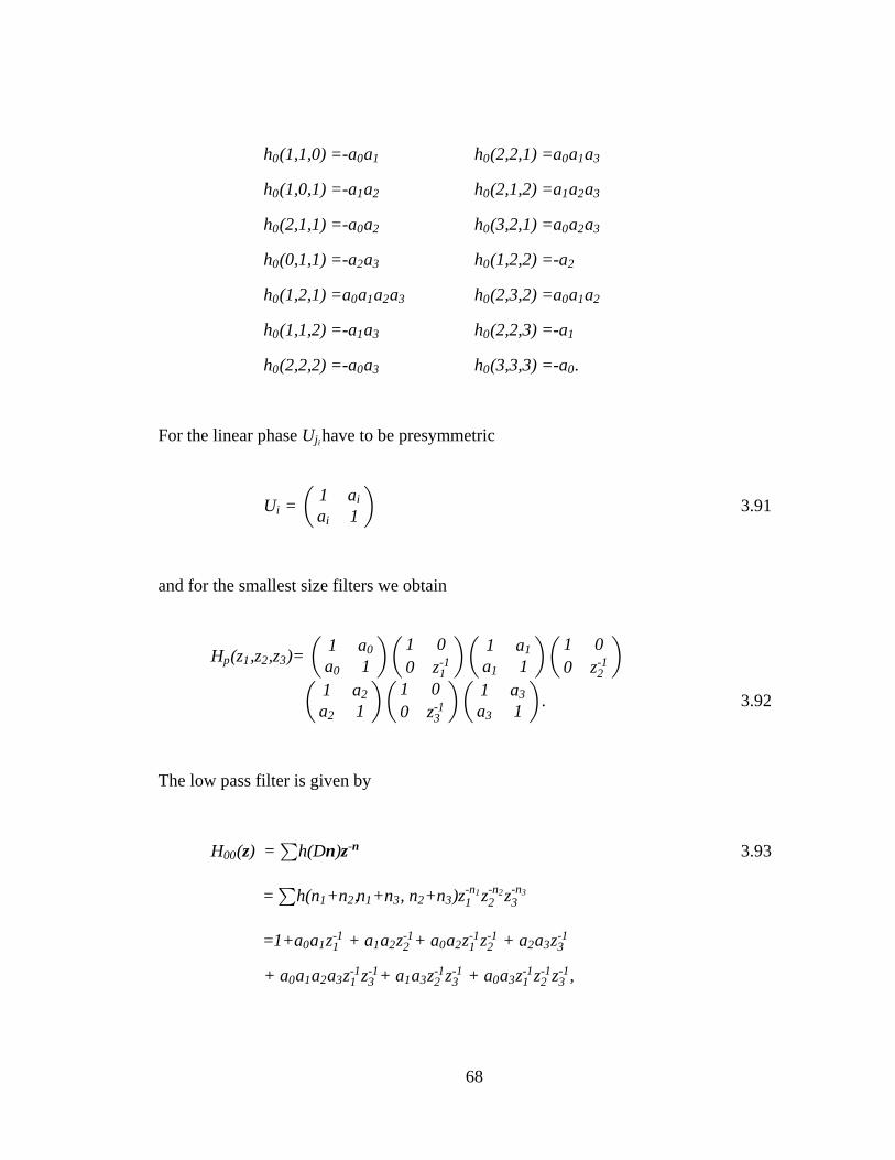
68

h (1,1,0) =-a a h (2,2,1) =a a a0 0 1 0 0 1 3

h (1,0,1) =-a a h (2,1,2) =a a a0 1 2 0 1 2 3

h (2,1,1) =-a a h (3,2,1) =a a a0 0 2 0 0 2 3

h (0,1,1) =-a a h (1,2,2) =-a 0 2 3 0 2

h (1,2,1) =a a a a h (2,3,2) =a a a0 0 1 2 3 0 0 1 2

h (1,1,2) =-a a h (2,2,3) =-a0 1 3 0 1

h (2,2,2) =-a a h (3,3,3) =-a .0 0 3 0 0

For the linear phase have to be presymmetricUji

3.91U = 1 aa 1i

i

iŒ

and for the smallest size filters we obtain

H (z ,z ,z )= 1 a 1 aa 1 a 1

1 0 1 00 z 0 zp 1 2 3

0 1

0 11 2-1 -1Œ Œ Œ Œ

3.92Œ Œ Œ1 a 1 aa 1 a 1

1 00 z .2 3

2 33-1

The low pass filter is given by

3.93H ( ) = h(D )00-z n z n

= h(n +n ,n +n , n +n )z z z1 2 1 3 2 3 1 2 3-n -n -n1 2 3

=1+a a z + a a z + a a z z + a a z0 1 1 2 0 2 2 31 2 1 2 3-1 -1 -1 -1 -1

+ a a a a z z + a a z z + a a z z z ,0 1 2 3 1 3 0 31 3 2 3 1 2 3-1 -1 -1 -1 -1 -1 -1

69

H (z) = h(Dn + k )z01 1-n

= h(n +n + 1,n +n +1, n +n +1)z z z1 2 1 3 2 3 1 2 3-n -n -n1 2 3

=a + a a a z + a a a z + a a a z z + a z +3 0 1 3 1 2 3 0 2 3 21 2 1 2 3-1 -1 -1 -1 -1

,a a a z z + a z z +a z z z0 1 2 1 01 3 2 3 1 2 3-1 -1 -1 -1 -1 -1 -1

is given by the following coefficientsh (n ,n ,n )0 1 2 3

h (0,0,0) =1 h (1,1,1) =a 3.940 0 3

h (1,1,0) =a a h (2,2,1) =a a a0 0 1 0 0 1 3

h (1,0,1) =a a h (2,1,2) =a a a0 1 2 0 1 2 3

h (2,1,1) =a a h (3,2,2) =a a a0 0 2 0 0 2 3

h (0,1,1) =a a h (1,2,2) =a 0 2 3 0 2

h (1,2,1) =a a a a h (2,3,2) =a a a0 0 1 2 3 0 0 1 2

h (1,1,2) =a a h (2,2,3) =a0 1 3 0 1

h (2,2,2) =a a h (3,3,3) =a .0 0 3 0 0

3.4.3 ORDER FILTER:N-1 to N

Generally higher order filters can be obtained by cascading basic blocks while

retaining perfect reconstruction property [40]. A higher order linear phase system can

also be derived from a lower order ones by choosing

3.95H (z) =H (z).D(z).Up pN N-1

where and is persymmetric(i.e. ).D(z) = z .JD(z)J U U=JUJ-k s

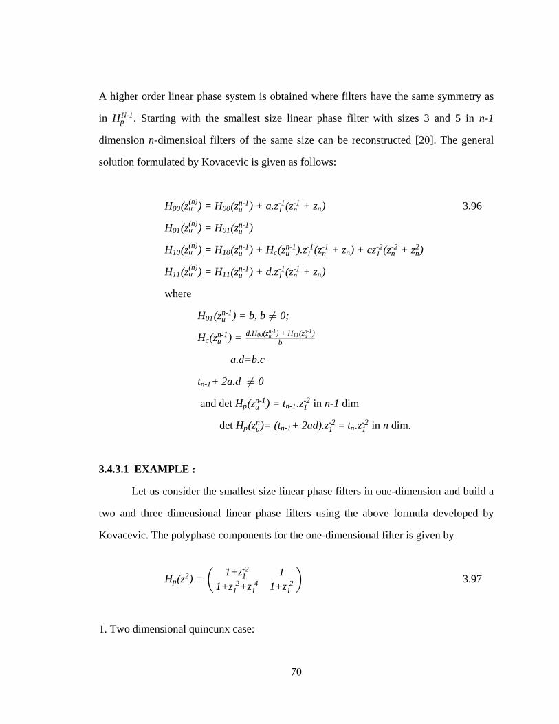
70

A higher order linear phase system is obtained where filters have the same symmetry as

in . Starting with the smallest size linear phase filter with sizes 3 and 5 in H n-1pN-1

dimension -dimensioal filters of the same size can be reconstructed [20]. The generaln

solution formulated by Kovacevic is given as follows:

3.96H (z ) = H (z ) + a.z (z + z ) 00 00 nu(n)

u nn-1 -1 -1

1

H (z ) = H (z )01 01u(n)

un-1

H (z ) = H (z ) + H (z ).z (z + z ) + cz (z + z )10 10 c nu(n)

u u n n nn-1 n-1 -1 -1 -2 -2 2

1 1

H (z ) = H (z ) + d.z (z + z )11 11 nu(n)

u nn-1 -1 -1

1

where

H (z ) = b, b 0;01 un-1 Á

H (z ) = c un-1 d.H (z ) + H (z )

b00 11u u

n-1 n-1

a.d=b.c

t + 2a.d 0n-1 Á

and det in dimH (z ) = t .z n-1p n-1un-1 -2

1

det = in dim.H (z )= (t + 2ad).z t .z np n-1 nun -2 -2

1 1

3.4.3.1 EXAMPLE :

Let us consider the smallest size linear phase filters in one-dimension and build a

two and three dimensional linear phase filters using the above formula developed by

Kovacevic. The polyphase components for the one-dimensional filter is given by

3.97H (z ) = 1+z 11+z +z 1+zp

2 1-2

1 1-2 -4 -2

1Œ

1. Two dimensional quincunx case:

71

To construct the two dimensional solution we need to determine

3.98H (z ) = d.(1+z ) + a.(1 + z )c 1 1 12 -2 -2

= (a+d)(1+z ).1-2

For the quincunx sampling matrix

3.99H (z z ,z z ) = 1 + z + az (z + z )00 1 1 2 22 1 1 2-1 -2 -1 -1

H (z z ,z z ) = 101 1 1 22-1

H (z z ,z z )=1+z +z +(a+d).(1+z )z (z +z )+ad.z (z +z )10 1 1 2 22 1 1 1 2 1 2 2-1 -2 -4 -2 -1 -1 -2 -2 2

1

,H (z z ,z z ) = 1 + z + dz (z + z )11 1 1 2 22 1 1 2-1 -2 -1 -1

, 3.100h (n ,n ) = 0 a 01 1 10 a 0

0 1 2Î ÑÏ Ò

. 3.101h (n ,n ) =

ada+d d a+d

1 1 1 1 1a+d d a+d

ad

0 1 2

Î ÑÐ ÓÐ ÓÐ ÓÐ ÓÏ Ò

! ! ! !! !

! !! ! ! !

2. Three-dimensional FCO case:

For the FCO sampling case, we start with the two dimensional linear phase filter

constructed above and using the same formula above the polyphase components of the

two filters are developed. First let us determine Hc

3.102H (z ) = c un-1 f.H (z ) + e.H (z )

H (z )00 11u u

n-1 n-1

01 un-1

= f.(1 + z + az (z + z )) + e.(1 + z + dz (z + z ))1 1 2 1 1 2-2 -1 -1 -2 -1 -1

2 2

= (e+f)(1+z ) + (af +de)z (z + z )1 1 2-2 -1 -1

2

72

3.103H (z ) =H (z ) + e.z (z + z )00 00 3D n-1 -1 -1

u 1 3FCO

=1 + z + az (z + z ) + e.z (z + z )1 1 2 1 3-2 -1 -1 -1 -1

2 3

H (z ) = H (z )00 01D n-1

uFCO

= 1

H (z ) = H (z ) + H (z ).z (z + z ) + ef.z (z + z )10 10 c 3D n-1 n-1 -1 -1 -2 -2 2

u u 1 3 1 3 3FCO

1+z +z +(a+d)(1+z )z (z +z )+ad.z (z +z ) = 1 1 1 2 1 2 2-2 -4 -2 -1 -1 -2 -2 2

1 2

+ (e+f)(1+z ) + (af +de)z (z + z )z (z + z ) +1 1 2 1 3-2 -1 -1 -1 -1

2 3

ef.z (z +z )1 3 3-2 -2 2

H (z ) = H (z ) + f.z (z + z )11 11 3D n-1 -1 -1

u 1 3FCO

=1 + z + dz (z + z ) + f.z (z + z ).1 1 2 1 3-2 -1 -1 -1 -1

2 3

The two filters and are shown in the Figure 3.15 below.h (n ,n ,n ) h (n ,n ,n )0 1 2 3 1 1 2 3

Figure 3.15: 3-D FCO HP and LP Filters

73

3.4.4 TRANSFORMATION:

Multidimensional filters can be designed using a transformation that maps one-

dimensional designs into multidimensional ones. ( See [13], [64], [70], [78], [79], [91])

Under these transformations perfect reconstruction and zeros at aliasing frequencies are

preserved.

3.4.4.1 SEPARABLE POLYPHASE COMPONENTS:

Multidimensional filter with separable polyphase components can be designed

with each polyphase component constituting products of one-dimensional filters. We start

with one-dimensional filter having polyphase components and construct -H (z) ni

dimensional components as

3.104H (z ,z ,... z ) = H (z ).H (z ) H (z ), i=0,1,2...i 1 2 n i 1 i 2 i nß â

Then the -dimensional filter with respect to the sampling lattice (with columnsn D

d , d1 náß ) is given by

. 3.105H(z ,z , z ) = z H (z ) H (z )1 2 n i ik U

-k d dáß âi c

t

i 1 n

%

The zeros of map into the zeros of .H(z) H(z ,z , z )1 2 náß

Let us consider the previous quincunx sampling and the following one-

dimensional linear phase filter with polyphase components

3.106H (z) = H (z) H (z)H (z) H (z)p

00 01

10 11” •

74

= ,” •1+6z +z 4+4z(1+z )

-2 -4 -2

1 416 16

-2

. 3.107” • ” •HH =

1+4z +6z +4z +z(1+4z +z )

0

1

-1 -2 -3 -4

116

-1 -2

The separable polyphase components are given by

3.108H (z ,z ) = H (z )H (z ), i=0,1i 1 2 i 1 i 2

H (z ,z ) = H (z )H (z )00 1 2 00 1 00 2

= 1+ 6z +6z +z +z +36z z +6z z +6z z +1 2 1 2 1 2 1 2 1 2-1 -1 -2 -2 -1 -1 -1 -2 -2 -1

z z1 2-2 -2

H (z z ,z z ) = H (z z )H (z z )00 1 1 2 00 1 00 1 22 2-1 -1

= 1+ 6z z + 6z z +z z +z z + 36z + 6z z +1 1 2 1 2 1 2 1 2-1 -1 -1 -2 2 -2 -2 -2 -3 -1

2 1

6z z + z1 1-3 -4

2

H (z ,z ) = H (z )H (z )01 1 2 01 1 01 2

= 16+16z +16z +16z z1 2 1 2-1 -1 -1 -1

H (z z ,z z ) = H (z z )H (z z )01 1 1 2 01 1 01 1 22 2-1 -1

= .16+16z z +16z z +16z1 1 2 1-1 -1 -1 -2

2

And the two dimensional lowpass filter is given by

. 3.109h (n ,n ) =

0 0 1 0 00 6 16 6 01 16 36 16 10 6 16 6 00 0 1 0 0

0 1 2

Î ÑÐ ÓÐ ÓÐ ÓÐ ÓÏ Ò

75

Let us extend the above linear phase filter to a three-dimensional filter with FCO

sampling and the separable polyphase components will be

3.110H (z ,z ,z ) = H (z )H (z )H (z ), i=0,1i 1 2 3 i 1 i 2 i 3

H (z ,z ,z ) = H (z )H (z )H (z )00 1 2 3 00 1 00 2 00 2

= 1+6z +6z +6z +z +z +z +36z z +36z z +1 2 3 1 2 3 1 2 1 3-1 -1 -1 -2 -2 -2 -1 -1 -1 -1

36z z +6z z + 6z z + 6z z + 6z z +2 3 1 2 1 2 1 3 1 3-1 -1 -1 -2 -2 -1 -1 -2 -2 -1

6z z + 6z z + z z + z z + z z +2 3 2 3 1 2 1 3 2 3-1 -2 -2 -1 -2 -2 -2 -2 -2 -2

36z z z + 36z z z +36z z z + 6z z z +1 2 3 1 2 3 1 2 3 1 2 3-1 -1 -2 -1 -2 -1 -2 -1 -1 -1 -2 -2

6z z z +6z z z +216z z z +z z z1 2 3 1 2 3 1 2 3 1 2 3-2 -1 -2 -2 -2 -1 -1 -1 -1 -2 -2 -2

3.111H ( ) = H (z z )H (z z )H (z z )00 00 1 00 1 3 00 2 3D

2z FCO

=1+6z z +6z z + 6z z + z z + z z + z z +1 2 2 3 1 3 1 2 2 3 1 3-1 -1 -1 -1 -1 -1 -2 -2 -2 -2 -2 -2

36z z z + 36z z z + 36z z z + 36z z z +1 2 3 1 2 3 1 2 3 1-1 -1 -2 -1 -2 -1 -2 -1 -1 -2 -3 -3

2 3

36z z z + 36z z z + z z z + z z z + z z z1 3 1 2 1 2 3-3 -2 -3 -3 -3 -2 -4 -2 -2 -2 -4 -2 -2 -2 -4

2 3 2 3 1 3 1 2

+ 6z z z + 6z z z + 6z z z + 6z z z +1 2 3 1 2 3 1 2 3 1-4 -3 -3 -3 -4 -3 -3 -3 -4 -3 -1 -2

2 3

6z z z + 6z z z + 6z z z +6z z z +1 2 2 3-3 -2 -1 -1 -3 -2 -2 -3 -1 -1 -2 -3

2 3 1 3 1 3 1 2

6z z z + 216z z z +z z z1 2 1 2 3-2 -1 -3 -2 -2 -2 -4 -4 -4

3 1 2 3

H (z ,z ,z ) = H (z )H (z )H (z )01 1 2 3 01 1 01 2 01 3

= 64+64z +64z + 64z + 64z z + 64z z +1 2 3 1 2 1 3-1 -1 -1 -1 -1 -1 -1

64z z + 64z z z2 3 1 2 3-1 -1 -1 -1 -1

H ( ) = H (z z )H (z z )H (z z )01 01 1 01 1 2 01 2 3D

2z FCO

= 64+ 64z z + 64z z + 64z z + 64z z z +1 2 2 3 1 3 1 2 3-1 -1 -1 -1 -1 -1 -2 -1 -1

64z z z + 64z z z + 64z z z .1 2 3 1 2 3 1 2 3-1 -2 -1 -1 -1 -2 -2 -2 -2

76

And the three-dimensional lowpass filter is given by with the followingh (n ,n ,n )0 1 2 3

coefficients:

h (0,0,0) =1 h (2,2,2) =216 0 0

h (0,1,1) =6 h (2,2,3) =640 0

h (0,2,2) =1 h (2,2,4) =10 0

h (1,0,1) =6 h (2,3,1) =60 0

h (1,1,0) =6 h (2,3,2) =640 0

h (1,1,2) =36 h (2,3,3) =360 0

h (1,2,2) =36 h (2,3,4) =640 0

h (1,2,2) =64 h (2,4,2) =10 0

h (1,0,1) =6 h (2,4,3) =640 0

h (1,1,0) =6 h (3,1,2) =60 0

h (1,1,2) =36 h (3,2,1) =60 0

h (1,2,2) =36 h (3,2,3) =360 0

h (1,2,2) =64 h (3,3,2) =360 0

h (1,0,1) =6 h (3,3,3) =640 0

h (1,2,3) =6 h (3,3,4) =6 0 0

h (1,3,1) =64 h (3,4,3) =60 0

h (1,3,2) =6 h (3,4,4) =640 0

h (2,0,2) =1 h (4,2,2) =1 0 0

h (2,1,1) =36 h (4,3,3) =6 0 0

h (2,1,3) =6 h (4,4,4) =1.0 0

h (2,2,0) =10

77

3.4.4.2 McClellan Transformation:

This transformation maps a single dimensional zero-phase filters into zero-phase

multidimensional filters (See [77],[90]). A linear phase filter can be written as

3.112H(z ,z ,...z ) = d.H ( , ,.... ),1 2 n sz + z z + z

2 2 2z + z1 21 2

-1 -1n n

-1

= pure delay. d

The idea of McClellan transformation is to replace the one-dimensional kernel

k(z)=( ) k(z ,z ,...z ) H( k(z ,z ,...z ))z + z2 1 2 n 1 2 n

1 1-1

by a multidimensional kernel . The filter

remains linear phase as long as is zero-phase. Perfect reconstruction andk(z ,z ,...z )1 2 n

zeros at aliasing frequencies are preserved. If the determinant of is monomial inH (k(z))p

one-dimension so is the determinant of and perfect reconstruction isH ( k(z ,z ,...z )) p 1 2 n

preserved. The zeros of order at in one-dimension maps into zeros of order at2N 2N1

( , ,... ) in .1 1 1 n-dimensions

3.4.4.3 EXAMPLE:

Let us consider the single dimensional linear phase filter given above (3.112).

Based on the McClellan transformation, we will construct the two-dimensional linear

phase filter for the quincunx case. The above filter can be written in terms of the kernel,

k(z), as follows

3.113H (z) = z H (k(z)),0 s-k

0

.H (z) = z H (k(z))1 s-l

1

Then the polyphase components of the filter can be expressed as

78

3.114H (z ) = z H (k(z)) = z 4+400 s2 -k -2 z + z

2

200

1 1-1” •Š ‹

H (z ) = z H (k(z)) = z 801 s2 -k+1 -1 z + z

2011 1

-1’ “Š ‹ H (z ) = z H (k(z)) = z10 s

2 -l -1 18 2

z + z10

1 1-1’ “Š ‹

H (z ) = z H (k(z)) = z11 s2 -l+1 0 4

1611‘

with

det H (z ) = z (P(k(z))-Q(k(z)))p2 -(k+l-1)

where P(k(z)) = H (k(z))H (k(z))s s00 11

Q(k(z)) = H (k(z))H (k(z)).s s10 01

Because perfect reconstruction holds

3.115P(k(z))= k +R(k(z)), Q(k(z)) = k + R(k(z)).1 2

If we define , the two-dimensional filters and their polyphasek(z ,z ) = 1 2z + z + z + z

2Š ‹1 21 2-1 -1

components are given by

3.116H (z ,z ) = z H (k(z ,z )) 00 1 2 s 1 21-k

00

= z 4+41-2 z + z + z + z

2

2” •Š ‹1 21 2-1 -1

= 1+6z +z +2z z +2z z + 2z z + 2z z + 2z z +1 1 1 2 1 2 1 2-2 -4 -1 -1 -1 -2 2 -2 -2 -3

1 12 2

2z z1-3 -1

2

H (z z ,z z )=1+6z z + z z + 2z + 2z + 2z + 2z + 2z z +00 1 1 22 1 2 2 1 1 2-1 -2 2 -4 4 2 -2 4 -4 -2 2

1 2 2 1

2z z1-4 2

2

H (z ,z ) = z H (k(z ,z ))01 1 2 s 1 21-k+1

01

=z 81-1 z + z + z + z

2’ “Š ‹1 21 2-1 -1

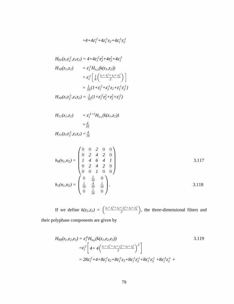
79

=4+4z +4z z +4z z1 1 1 2-2 -1 -1 -1

2

H (z z ,z z ) = 4+4z z +4z +4z01 1 1 22 1 2 2 1-1 -2 2 2 -2

H (z ,z ) = z H (k(z ,z ))10 1 2 s 1 21-1

10

= z1-1 1

8 2z + z + z + z’ “Š ‹1 21 2

-1 -1

= 116 1 1 1 2

-2 -1 -1 -12(1+z +z z +z z )

H (z z ,z z ) = (1+z z +z +z )10 1 1 22 1 2 2 1-1 -2 2 2 -21

16

H (z ,z ) = z H (k(z ,z ))11 1 2 s 1 21-1+1

11

= 416

H (z z ,z z ) =11 1 1 22-1 4

16

3.117h (n ,n ) =

22 4 2

1 4 6 4 12 4 2

1

0 1 2

Î ÑÐ ÓÐ ÓÐ ÓÐ ÓÏ Ò

! ! ! !! !

! !! ! ! !

. 3.118h (n ,n ) = 1 1 2

116

1 4 116 16 16

116

Î ÑÐ ÓÏ Ò

! !

! !

If we define , the three-dimensional filters andk(z ,z ) = 1 2z + z + z + z + z + z

2Š ‹1 2 31 2 3-1 -1 -1

their polyphase components are given by

3.119H (z ,z ,z ) = z H (k(z ,z ,z )) 00 1 2 3 s 1 2 31-k

00

=z 4+ 41-2 z + z + z + z + z + z

2

2” •Š ‹1 2 31 2 3-1 -1 -1

= 28z +4+8z z +8z z +8z z +8z z +8z z +1 1 1 1 2 1 3 2-2 -1 -1 -1 -1 -1 -1 -3 -1

2 3 1

80

8z z + 8z z + 4z z + 8z z z + 8z z z +1 1-3 -3 -1 -2 2 -2 -2 -1

3 2 3 23 1 2 1 1 3

8z z z +8z z z + 4z z + 4z z + 8z z +1 2 1 2 3 2 3 1 2-2 -1 -2 -1 -1 -2 2 -2 -2 -3

3 2 3

4z z + 4z1 3-2 -2 -4

1

H (z ,z ,z ) = z H (k(z ,z ,z ))01 1 2 3 s 1 2 31-k+1

01

=z 81-1 z + z + z + z + z + z

2’ “Š ‹1 2 31 2 3-1 -1 -1

= 4 +4z + 4z z + 4z z + 4z z + 4z z-2 -1 -1 -1 -1 -1 -11 1 1 2 1 1 32 3

H (z ,z ,z ) = z H (k(z ,z ,z ))10 1 2 3 s 1 2 31-1

10

=z1-1 1

8 2z + z + z + z + z + z’ “Š ‹1 2 31 2 3

-1 -1 -1

= 116 1 1 1 2 1 1 3

-2 -1 -1 -1 -1 -1 -12 3(1+z + z z + z z +z z +z z )

H (z ,z ,z ) = z H (k(z ,z ,z ))11 1 2 3 s 1 2 31-1+1

11

= 416

H ( ) =28z z +8z z +8z z z + 8z z z +8z z z +00 3D -2 -2 -1 -3 -1 -2 -1 -3 -2 -2 -1 -1

1 2 1 1 2 3 2 1 2 31z FCO

8z z z + 8z z z +8z z + 4z z + 4z z z +4+1 3 2 2 3-2 -3 -4 -3 -1 -3 -1 -4 -4 -4 -2 2

2 1 2 1 1 2 13

4z z + 4z z + 4z z z +8z z +8z z + 8z z z2 3 1 3 1 2 1-2 2 -2 2 -2 -4 -2 -1 -1 -3 -4 -1

2 1 23 3

+ 8z z z1 2 3-1 -1 2

H ( ) = 4 +4z z + 4z z + 4z z z + 4z z + 4z z z01D -2 -2 -1 -2 -1 -1 -1 -1 -2 -1

1 2 2 1 2 3 1 1 2 33 3z FCO

H ( ) = (1+z z + z z + z z z +z z +z z z )10D -2 -2 -1 -2 -1 -1 -1 -1 -2 -11

16 1 2 2 1 2 3 1 1 2 33 3z FCO

H ( ) = .11D 4

16z FCO

3.5 SUMMARY

The basic concepts in multidimensional multirate filter banks have been

described. Several methods for the construction of multidimensional filters have been

81

outlined. Even though several methods exist for building these filter banks much more

emphasis has been placed on cascade structures for their simplicity of construction. The

satisfaction of regularity condition is essential in generating continuous wavelets bases

from these multidimensional filter banks. The method of generating regular

multidimensional filter banks will be the topic of the subsequent chapter.

82

CHAPTER 4

ON THE REGULARITY OF MULTIDIMENSIONAL NON-SEPARABLE

CASCADE FILTER BANKS

4.1 INTRODUCTION:

The satisfaction of regularity condition is essential in generating continuous

wavelet bases from iterated filter banks. In one-dimension regularity of filters is

guaranteed by packing zeros at the aliasing frequencies [25],[45]. In multiple dimensions

the same could be done, but care must be made to keep the perfect reconstruction

requirement simultaneously. In the case of transformation of one dimensional to

multidimensional filterbanks, the zeros at aliasing frequencies of the starting filters are

preserved. It is therefore essential to design the single dimensional filters with sufficient

regularity. With cascade filters the perfect reconstruction requirement is structurally

included and the zeros at aliasing frequencies are imposed algebraically using the

undetermined coefficients. In what follows the regularity of cascade structures are

discussed in detail.

4.2 REGULARITY:

As mentioned previously the satisfaction of regularity condition is necessary to

generate continuous wavelet bases from iterated filter banks. In case of one-dimensional

filters this condition is guaranteed by packing zeros at the aliasing frequencies. (See [21],

[84]). A sufficiently high order of zeros are imposed at aliasing frequencies (or points of

repeated spectra). In multiple dimensions, the same could be applied, i.e. impose a zero

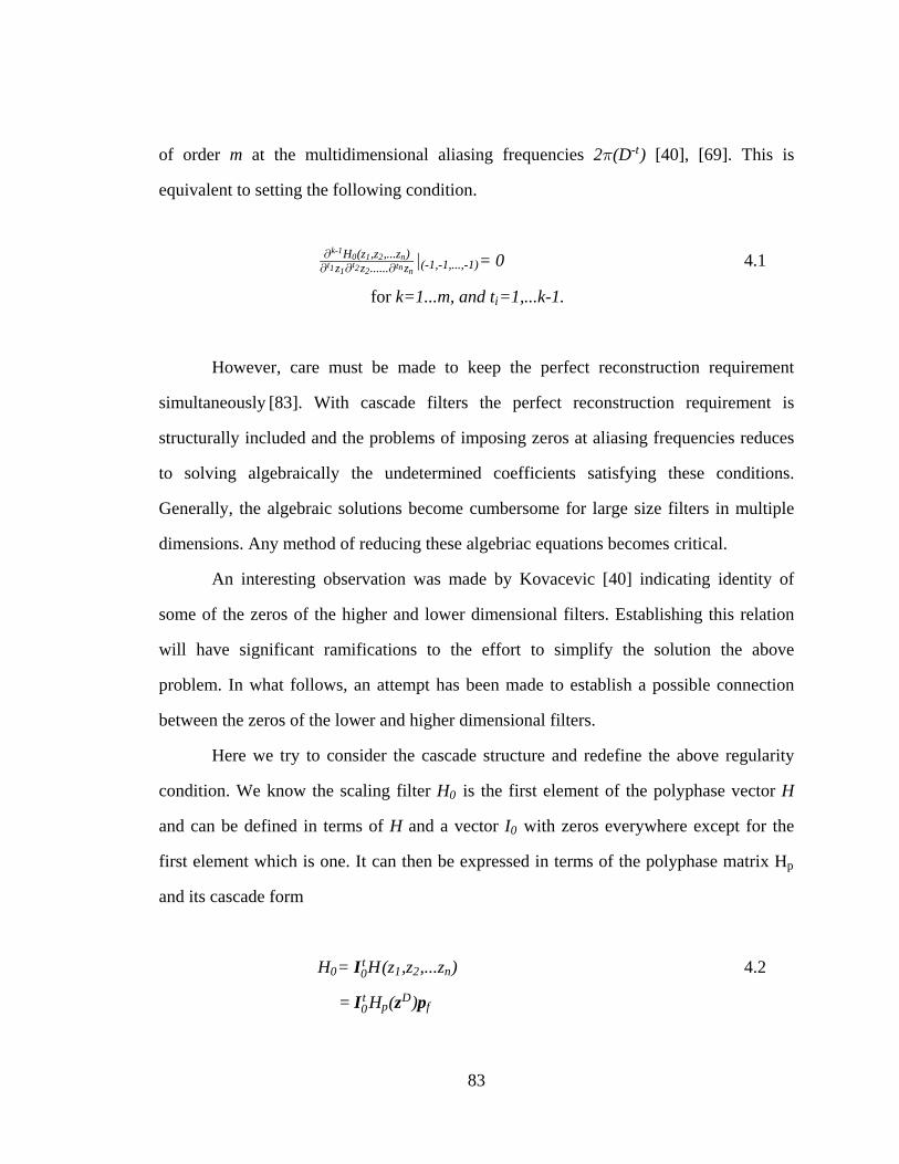
83

of order at the multidimensional aliasing frequencies [40], [69]. This ism 2 (D ) 1 -t

equivalent to setting the following condition.

4.1`` ` `

k-10 1 2 n

t t1 21 2 ntnH (z ,z ,...z )

z z ...... z (-1,-1,...,-1)l = 0

for k=1...m, and t =1,...k-1.i

However, care must be made to keep the perfect reconstruction requirement

simultaneously [83]. With cascade filters the perfect reconstruction requirement is

structurally included and the problems of imposing zeros at aliasing frequencies reduces

to solving algebraically the undetermined coefficients satisfying these conditions.

Generally, the algebraic solutions become cumbersome for large size filters in multiple

dimensions. Any method of reducing these algebriac equations becomes critical.

An interesting observation was made by Kovacevic [40] indicating identity of

some of the zeros of the higher and lower dimensional filters. Establishing this relation

will have significant ramifications to the effort to simplify the solution the above

problem. In what follows, an attempt has been made to establish a possible connection

between the zeros of the lower and higher dimensional filters.

Here we try to consider the cascade structure and redefine the above regularity

condition. We know the scaling filter is the first element of the polyphase vector H H0

and can be defined in terms of and a vector with zeros everywhere except for theH I0

first element which is one. It can then be expressed in terms of the polyphase matrix Hp

and its cascade form

4.2H = H(z ,z ,...z ) 0 1 2 n0tI

= I z p0t D

p fH ( )

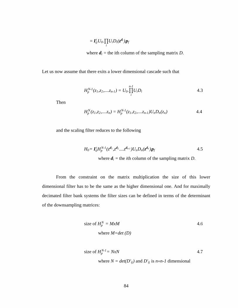
84

= U . U D ( ).I z p0t

0 i i fi

# di

where = the ith column of the sampling matrix .di D

Let us now assume that there exits a lower dimensional cascade such that

4.3H (z ,z ,....z ) = U . U D pN-1

1 2 n-1 0 i ii

n-1# Then

4.4H (z ,z ,....z ) = H (z ,z ,....z )U D (z )p pN N-1

1 2 n 1 2 n-1 n n n

and the scaling filter reduces to the following

4.5H = H (z ,z ....z )U D ( ).0 n n f0t N-1

pI z pd d d d1 2 n-1 n

where = the th column of the sampling matrix .di i D

From the constraint on the matrix multiplication the size of this lower

dimensional filter has to be the same as the higher dimensional one. And for maximally

decimated filter bank systems the filter sizes can be defined in terms of the determinant

of the downsampling matrices:

size of 4.H = MxM pN '

where M=det (D)

size of 4.H = NxNpN-1 (

where and is dimensionalN = det(D' ) D' n n-1ij ij ‡

85

submatrix of .D

From the definition of the determinant of and the multiplicative constraint onD

the matrices above

4.det(D)=M= d D = det(D )= N.j

ij' 'ij ijl l )

If there exists a submatrix of having the same determinant as then thereD' D D

are a series of unimodular transformations that reduce to the following forms.D

4.D

d 0 d0

0 0 d 0 00

d 0 d

´

Î ÑÐ ÓÐ ÓÐ ÓÐ ÓÏ Ò

11 1n

ij

n1 nn

*

or

. 4.D D' 00 d´ Œ

nn"!

These unimodular transformations of the sampling matrix would not alter the

sampling pattern. The coset vectors and the forward polyphase transform remain also the

same. Substituting this into the above , we obtainH0

4.1H = H ( )U D ( ).0 n n f0t N-1 D' d

p n(n-1)I z z pnn "

where is the dimensional index . z z(n-1) n-1

86

The forward polyphase transform in dimensions can be expressed in terms ofN

the corresponding forward polyphase transform in dimensions.N-1

4.1p p f fN N-1

n=T(z ) #

where T=

z

z

Î ÑÐ ÓÐ ÓÐ ÓÐ ÓÏ Ò

nk

nk

1

n

ÞÞ

Þ

is matrix of delays along the th dimension. n n n‡

Finally substituting the above term into the scaling filter gives

4.1H = H (z )U D (z )T(z )0 n n n0t N-1 D' d N-1

p n(n-1) fI pnn Þ $

The regularity condition can be rewritten as

4.1`

` ` `

k-1 t N-1 D' d N-10 (n-1)p nn n nnn

ft t1 21 2 ntn

I pH (z )U D (z )T(z )z z ...... z (-1,-1,..-1)l = 0 %

`

` ` `

k-1 t N-1 D' N-10 (n-1)p f

t t1 21 2 ntn

I pH (z )Q.z z ...... z (-1,-1,..-1)l = 0,

where Q(z ) = U D (z )T(z )n n n nndnn

i=1

ni it = k-1, t [0..k-1].%

For the special case where equals zero this reduces totn

4.15`

` ` `

k-1 t N-1 D' N-10 (n-1)p f

t t1 21 2 n-1tn-1

I pH (z )Q.z z ...... z (-1,-1,...-1)l = 0,

87

where i=1

n-1i it = k-1, t =0..k-1.

One way of approaching the problem is to redefine a new dimensionalN-1

forward polyphase transform as

4.1p p .f fN-1 N-1= Q. '

Then the regularity condition reduces to

4.1`

` ` `

k-1 t D' N-10 (n-1)

N-1p f

t t1 21 2 n-1tn-1

I pH (z )z z ...... z (-1,-1,...-1)l = 0. (

Thus for some forward polyphase transfer function the dimensional filterpfN-1, n-1

satisfies the regularity condition. Because is a nonsingular unimodular matrixQ=U D T N N

at the transformation is one-to-one. Thus if are elements ofz =-1 =Q n f f f fN-1 N-1 N-1 N-1p p p , p

linear spaces respectively then these linear spaces are isomorphic. And if L, L =* N-1fp

Q Hp p pf f fN-1 N-1 N-1 N

pis an element of the null space of so is and by the same reasoning so is .

Thus some of the zeros of are shown also to be zeros of [39]H Hp pN-1N Þ

An alternative approach to show the above relation would be to use the concepts

of matrix fraction description of a polynomial transfer function [35] A rationalH(z) Þ

polynomial matrix can be written as

. 4.1H(z) = N(z)d(z) )

The transfer function can be defined using right or left matrix fractionH(z)

descriptions.

4.1H(z) = N(z)D (z) or D (z)N(z).R L-1 -1 *

88

Let us now consider the following two definitions which are the result of

generalizations of 2- polynomial matrices to the cases by Z. Lin [48], [49].D n-D

Definition 5.1:

Let be full normal rank, with Then is said to beA(z) C [z] m l. A(z)% mxl  

primitive in if for all fixed is ofC[z ][z ,...z ] z C, A(z , z , ...z ) C [z ,z ,...z ]1 2 n 11 11 2 n 1 2 nmxl% %

full normal rank.

Definition 5.2:

Let be of full normal rank, with the g.c.d. of allA(z) C [z] m l ; A(z) C[z]% %mxl  

the minors of and the content of . We say that has alxl A(z) g(z ) C[z ] A(z) A(z)1 1%

primitive factorization in if for some C[z ][z ,...z ] A(z) = L(z)R(z) L(z) C [z], R(z) 1 2 nmxl% %

C [z] R(z) = g(z ) L(z) C[z ][z ,..z ].mxl1 1 2 n with det , and being primitive in

The existence of the primitive factorization implies the uniqueness of moduloL(z)

a right unimodular matrix and modulo a left unimodular matrix. Hence the invariantR(z)

polynomials of and that determine the poles and zeros of are not affectedL(z) R(z) A(z)

by unimodular transformations.

Let us now consider the following factor in the scaling filter

4.A(z) = H (z )Q(z )pN-1 D'

(n-1) n #!

where and L(z) = H (z ) R(z) = Q(z ).pN-1 D'

(n-1) n

By construction satisfies the condition for existence of primitiveA(z) = L(z)R(z)

factorization and hence the finite poles and zeros of are unchanged by theA(z)

unimodular transformation. We know that is unimodular when evaluated at Q(z ) z =-1n n

and let

89

4.2P = Q(z ) -1n z =-1

¸n

"

A (z) = H (z )P.Q(z )* N-1 D'p (n-1) n Þ

A (z) A(z)* is equivalent to and substituting in equation 4.15 we get an equivalent relation

4.2`

` ` `

k-1 t N-1 D' N-10 (n-1)p f

t t1 21 2 n-1tn-1

I pH (z )z z ...... z (-1,-1,...-1)l = 0 #

where i=1

n-1i it = k-1, t =0..k-1Þ

Thus some of the zeros of the higher dimensional filers are shown to be zeros of

the lower dimensional filters [6]. This result has significant importance in devising

methods for the construction of higher dimensional regular filters from lower

dimensional ones.

4.3 TWO-CHANNEL CASE:

Here we restrict our discussion to uniform band, maximally sampled filter banks,

in which all the channels share the same downsampling matrix D with determinant equal

to two. These sampling matrix are nonseparable and reduce to quincunx and Face-

Centered Orthorhombic (FCO) cases in two and three dimensions respectively. The

analysis filters can be written as

4.2H( ) = H ( ). z z pp f $

where H( ) =[H ( ) , H ( )]z z z0 1t

coset vectorsp = z z kf it[ ] , = k k0 1 Þ

90

The perfect reconstruction filter bank with FIR analysis and synthesis filter has to

satisfy the condition

4.2det(H ( )) = c p z zd %

where is a delay vectord Þ

For the two channel -dimensional case the following cascade will producen

perfect reconstruction set containing two filters of the same size

4.25H ( ) = U U 1 00 zp 0 ij

j=1i=1

k n

i-1z ##Œ

is unitary for the orthogonal case, i.e.U ij

U = 1 a-a 1i1,2

11+a

i1,2

i1,2É i1,22 Œ

and

is persymmetric for the linear phase case i.eU .ij

U = .1 aa 1i1,2

11+a

i1,2

i1,2É i1,22 Œ

For the smallest size filters this reduces to

4.2H ( ) = U U ,1 00 zp 0 i

i=1

n

i-1z #Π'

91

where equals unitary for orthogonal and persymmetric for the linear phase caseU i

and the polyphase components of the analysis filters are given by

4.2H( ) = H ( ). z z zzp

D ” •k

k

0

1(

= U U . 1 00 z0 i

i=1

n

i-d#Œ ” •i

0

1

zz

k

k

= . .1 a-a 1

1 a-a z zŒ Œ ” •#0

0 i=1

n i

i i i-d -di i

0

1

zz

k

k

The scaling filter is given by the first row of the above vector and the aboveH0

regularity condition is defined by

4.2`` ` `

k-10

t t1 21 2 n-1tn-1

Hz z ...... z (-1,-1,...-1)l =0 )

`` ` `

k-10

t t1 21 2 n-1tn-1

I H( ) z z ...... z (-1,-1,...-1)

z l = 0.

As stated above some of the zeros of the higher dimensional filters constitute also

the zeros of the lower dimensional filters. This is illustrated by the following examples.

4.3.1 EXAMPLE:

Let us examine the quincunx and FCO cases for the sampling matrices given in

[42].

, . 4.2D = D =1 1-1 1

1 1 1-1 -1 10 -1 1

q FCOŒ Î ÑÏ Ò *

92

For the above given sampling matrix the following 2- polyphase cascadeD Dq

matrix is obtained.

4.H (z ,z ) = U1 0 1 00 z 0 zU Up 1 02

i=1

k

1 21 2” •#Œ Œi i $!

and for the orthogonal filters have to be unitary i.e.Uji

U = .1 -aa 1j

11+a

i

ii

i2É Œ

For the case of the smallest size filter we obtain

4.3H (z ,z ) = U D U D Up 1 2 2 2 1 1 0 "

=d. ..1 -a 1 0 1 -aa 1 0 z a 1

1 00 zŒ Œ Œ Œ2 1

2 1 1 2

.. 1 -aa 1Π0

0,

where . d= 1

(1+a )Ë#i=0

2

i2

The polyphase components are given by

H( ) = d. ..1 a 1 a-a 1 -a 1

1 0 1 00 z 0 z

z Œ Œ Œ Œ0 1

0 11 2-d -d1 2

.. 1 a-a 1Œ ” •2

2

zz

k

k

0

1 4.3#

where p zzf

1-1= = .1z” • ” •k

k

0

1

The 2nd order regularity condition is given by

93

4.3`` `

1 t0

t t1 21 2

I zH( )z z (-1,-1)l = 0 $

where i

2i it = 1, t =0..1,

and the zeros of H determined by the direct algebraic method are given by0

4.3a =-2 3 a = 3 a = 30 1 2… „ „È È È %

a =-2 3 a = 0 a = 3.0 1 2„ „È È

For FCO sampling matrix the cascade structure generates the followingDFCO

filters

. 4.3H (z ,z ,z ) = U U1 0 1 00 z 0 zU U

1 00 zp 1 2 3 0 3

i=1

N-1

1 2-1 -11 2

3-1” •#Œ Œ Œi i i &

Again the orthogonal filters have to be unitaryUji

U = .1 -aa 1i

11+a

i

iÉ i2 Œ

And for the smallest size filters we get

H (z ,z ,z ) = d. ...1 -a 1 -aa 1 a 1

1 0 1 00 z 0 zp 1 2 3

0 1

0 1-1 -11 2

ΠΠΠΠ, 4.3.. 1 -a 1 -a

a 1 a 11 00 zŒ Œ Œ2 3

2 33-1 '

. where d= 1

(1+a )Ë#i=0

3

i2

The polyphase components are given by

94

H( ) = d. ...1 -a 1 -aa 1 a 1

1 0 1 00 z 0 zz Œ Œ Œ Œ0 1

0 1-d -d1 2

. 4.3... 1 -a 1 -aa 1 a 1

1 00 zŒ Œ Œ ” •2 3

2 3-d3

0

1

zz

k

k (

The 2nd order regularity condition for the 3- FCO is given byD

4.38`` ` `

1 t0

t t1 21 2 3t3

I Hz z z (-1,-1,-1)l = 0

where .i

3i it = 1, t =0..1

The solutions to the above equation determined by direct algebraic method are

given by

4.3 a =0 a = -2 3 a =0 a = 30 1 2 3„ „È È *

a =0 a =-2 3 a = 3 a = 3.0 1 2 3… … „È È È

Some of the solutions are the same as those given above for the 2- case. ThisD

relation between the 3- and 2- zeros can be reestablished using the result and methodD D

developed above.

First, we know the sampling pattern is not affected by the unimodular

transformation of the sampling matrix .DFCO

4.D = 1 1 1 1 -1 0-1 -1 1 1 3 -40 -1 1 1 1 0

'FCO

Î Ñ Î ÑÏ Ò Ï Ò"

# %!

95

= Î ÑÏ Ò

1 1 0-1 1 00 0 1

= .ΠD 00 1

q

Rewriting the polyphase components of the 3- filters with the new samplingD

matrix we get

4.4H( ) = d. ..1 -a 1 -aa 1 a 1

1 0 1 00 z 0 zz Œ Œ Œ Œ0 1

0 1-d -d1 2

"

.. 1 -a 1 -aa 1 a 1

1 00 zŒ Œ Œ ” •2 3

2 3-d3

0

1

zz

k

k

= H (z )d .1zp

(N-1) D3

1-1

q Œ Œ1 00 z

1 -aa 13

-13

3” •

where d = 31

(1+a )É 32

.

The scaling filter is given byH0

4.42H = I H( )0 0 z

= I H (z )d . .1z0 3p

(2) D

1-1

q Œ Œ1 00 z

1 -aa 1-1

3

3

3” •

The zeros of on the constant hyperplane of = -1 is given by the zeros ofH z0 3

4.4H = I H (z )d .1z0 0 3p

(2) D

1-1

q Œ Œ1 0 1 -a0 -1 a 1

3

3” • $

96

= . I H (z )d .1z0 3p

(2) D

1-1

q Π1 -a-a -1

3

3” •

The regularity condition can then be written as

4.4`` `

k-10

t t1 21 2

Hz z (-1,-1)l = 0 %

`

` `

k-10

(2)p (2)

Dqf

t t1 21 2

I pH (z ).Q.z z (-1,-1). = 0l

where ,Q = d . 1 -a-a -13

3

3Œ

i

2i it =k-1, t =0 k-1.ßá ß

Because is unimodular and equals , this will reduce to the followingQ p pfN-1

f

equation according to the above derived relationship.

4.4`

` `

k-10

(2)p (2)

Dqf

t t1 21 2

I pH (z ).z z (-1,-1)l = 0 &

where i

2i it =k-1, t =0..k-1.

For the 2nd order regularity condition

4.4`

` `

10

(2)p (2)

Dqf

t t1 21 2

I pH (z ).z z (-1,-1)l = 0 '

where t =1, t =0..1.i

2i i

This is identical to equation (4.43), which is the regularity condition for the

quincunx case above. Some of the zeros of the the higher dimensional FCO filters are

shown to be the same as the zeros of the lower dimensional quincunx filters.

97

In fact, the 2nd order zeros determined directly form equation (4.45) above for a3

arbitrary are given by

4.4a = 2 3 a = 0 a = - a =a ! " # $ $„ „

„È 4a -2a 3 + a (2 3)-1+3a

$# #$ $

#$

È È(

a = 2 3 a = 3 a = a =a .! " # $ $„ „

„ „È È -2a -4a 3+a ( 2 3)-1+3a

# #$ $$

#$

È È

And for values of away from the singular values of we obtain identicala a ,$ #

values as those determined algebraically for the 2- quincunx case above.D

4.4 CONSTRUCTION OF REGULAR CASCADE FILTERS:

I proved above that some of the zeros of the higher dimensional filters are also

zeros of the lower dimensional filters. I try to exploit this relation to build higher-

dimensional regular filters from lower-dimensional regular filters. Starting with lower

dimensional filters we will build higher dimensional regular filers recursively. In so

doing we will be able to reduce the number of undetermined coefficients and the

complexity of the algebraic solution. Let us assume that the zeros of the lower-

dimensional filters have been determined using the relation (4.14). Hence the coefficients

a a0 n-1á are determined. Substituting these values into equation (4.13) the only

undetermined coefficients will be . But an

4.4`

` ` ` áß

k-1 t N-1 D' d N-10 (n-1)p nn n nnn

ft t1 21 2 ntn

I pH (z )U D (z )T(z )z z ...... z (-1,-1, -1)l = 0 )

and if we assume =0, then this will reduce tot t1 n-1á

4.4`

` ß

k-1 t N-1 D' d N-10 (n-1)p nn n nnn

ftn n

I pH (z )U D (z )T(z )z (-1,-1,... -1)l = 0 *

I p0 (n-1)t N-1 D' k-1 d N-1

p nn n nnnf

tn n

H (z ) U D (z )T(z )z (-1,-1, -1)

`

` áßl = 0

where t =0 k-1.n á

98

The above equations will be sufficient to solve a and hence complete then

determination of all of the coefficients of the scaling filter.

4.4.1 EXAMPLE

Let us construct 3- scaling filter for the FCO sampling matrix using the aboveD

technique. Since the determinant of the FCO sampling matrix is 2 the submatrices

considered at every stage of the construction must have the also the same value. We start

with the single dimensional two channel filter with sampling rate equal to 2.

Figure 4.1: Extension From One To Multiple Dimension

4.H =U D U p 0 1 1 &!

=Œ Œ Œ1 -a 1 -aa 1 a 1

1 00 z

0 1

0 11-1

H = I H (z )0 p f0t 2

1 p

= I 1 -a 1 -aa 1 a 1

1 0 10 z z0

t 0 1

0 11 1-2 -1Œ Œ Œ Œ

where . p = [1 z ]f 1-1 t

99

The 2nd order regularity condition is given by

4.5``

k-10

t1 1 1Hz (z =-1)l = 0 "

where t =0 1 k=1 2.i á á

The solution to this problem is given by

4.5a =-2 3 a = 3 .0 1„ „È È #

Let us then consider the two-dimensional case with the submatrix

. 4.5D = 1 1-1 12 Π$

The polyphase matrix for the two dimensional case will be

4.5H =U D U D Up 0 1 1 2 2 %

= ,Œ Œ Œ Œ Œ1 -a 1 -a 1 -aa 1 a 1 a 1

1 0 1 00 z 0 z

0 1 2

0 1 21 2-1 -1

and the scaling filter will be

4.5H = I H (z )0 p f0t 2

1 p &

= I ..1 -a 1 -aa 1 a 1

1 0 1 00 z 0 z0

t 0 1

0 11 2-2 -1Œ Œ Œ Œ

.. ,1 -aa 1

1zŒ Œ2

2 1-1

where p = [1 z ] .f 1-1 t

The 2nd order regularity condition

100

4.5`` `

k-10

t t1 21 2 1 2H

z z (z =-1,z =-1)l = 0 '

where t =1, t =0..1 k=1..2.i

2i i

The solution to the above given the coefficients and will bea a0 1

4.5a =-2 3 a = 3 a = 0 0 1 2„ „È È (

a =-2 3 a = 3 a = 3 .0 1 2… „ „È È È

And finally the solution to 3- filter coefficients using the above technique andD

previously determined coefficients is

4.5a =-2 3 a = 3 a = 0 a = 2 3 0 1 2 3„ „ „È È È )

a =-2 3 a = 3 a = 3 a = 2 3.0 1 2 3… „ „ „È È È È

The solution above is identical to that determined by directly solving the equation

below.

4.59 `` ` `

k-10

t t t1 2 21 2 2 1 2 3H

z z z (z =-1,z =-1,z =-1)l = 0

where i

3i it =1, t =0..1 k=1..2.

As you may observe the number of solutions increases as the dimensions increase.

4.5 SUMMARY:

The work shows that some of the zeros of higher dimensional cascade filters are

related to the zeros of their lower dimensional cascade component filters. This relation is

101

exploited to develop a method for the construction of multidimensional regular filter

banks recursively. Starting form lower dimensional regular filters it is possible to build

higher dimensional filters with the same degree of regularity. In the next chapter I will

utilize these relation to outline practical procedure for the recursive construction of

regular multidimensional filters and compactly supported multidimensional wavelets.

102

CHAPTER 5

DESIGN OF MULTIDIMENSIONAL NON-SEPARABLE WAVELETS

5.1 INTRODUCTION:

The wavelet theory and its connection to multirate filter banks was first described

for the one-dimensional case by Mallat and Daubechies et al. in [21], [53], [54]. The

perfect reconstruction filter banks computes the discrete-time wavelet transform when the

branch with the low-pass filter is iterated. It was also shown that continuous wavelet

bases could be obtained by iterating regular low pass filters. The same basic ideas can be

applied in multiple dimensions with some major modifications. In the one-dimensional

case there are several techniques to design regular filter banks and in the last chapter I

have discussed techniques for the design of multidimensional regular filter banks. The

final aim is to construct continuous multidimensional wavelet bases by iterating these

regular multidimensional filter banks. Here in this chapter I discuss the methods for the

construction of multidimensional wavelet in general and the iterated filter bank method in

particular.

5.2 TENSOR PRODUCT OF ONE DIMENSIONAL BASIS:

5.2.1 TENSOR PRODUCT OF ONE DIMENSIONAL WAVELETS

The most trivial way of constructing multidimensional wavelet basis for , isL (R )2 n

simply to take the tensor product functions generated by one-dimensional bases [20].n

Let the orthonormal wavelet bases be defined asn

103

5.1< < %j,k- -j 2(x) = 2 (2 x-k) L (R).

j2

Then the tensor product wavelet is given by

5.2 < < < <j ,k ;j ,k ;.......j ,k 1 2 n j ,k j ,k ......... j ,k1 1 2 2 n n 1 1 2 2 n n.(x ,x ,....x ) =

The resulting functions are wavelets, and an orthonormal basis for . In this L (R )2 n

basis, the variables are dilated separately. x , x ,...,x1 2 n

5.2.2 TENSOR PRODUCT OF ONE DIMENSIONAL MRA:

Another construction is one in which the dilation of the resulting orthonormal

wavelet basis control all the variables simultaneously [20]. In this construction the tensor

product of one-dimensoinal multiresolution analysis is considered. Define the space n ,Vj

j Z% , by

5.3V0 0 0 0 = V V ... V Œ Š

= span F(x ,x ,...,x )1 2 n

= f (x )f (x )...f (x ) f , f ,...,f V1 1 2 2 n n 1 2 n 0%

and

5.4F F(2 .,2 .,....2 ) .% %V Vj 0j j jÍ

Then the form a multiresolution ladder in and satisfy the followingVj2 nL (R )

conditions:

104

5.5.... ... V V V V V2 1 0 -1 -2§ § § §

+j Z

= %

9Vj

-j Z

= L (R ).%

Vj2 n

Because the constitute an orthonormal basis for the product9 %(.,- ), n Z V ,n 0

functions

5.6F0;n ,n ,...n 1 2 n 1 1 2 2 n n1 2 n(x ,x ,....x ) = (x -n ) (x -n )... (x -n )9 9 9

n ,n ,..n Z,1 2 n %

constitute an orthonormal basis for , generated by -translations of a single functionV0nZ

F. Similarly, the

5.7F0;n ,n ,...n 1 2 n j,n j,n j,n1 2 n 1 2 n(x ,x ,....x ) = .... 9 9 9

n ,n ,..n Z1 2 n %

constitute an orthonormal basis for . As in the one-dimensional case, I define for each Vj j

% Z , the complement space to be the orthogonal complement in of i.e.W V Vj j-1 j

5.8V V Wj-1 j j = Š

and

5.9Šj Z

= L (R ) .%

FFWj2 n

105

The space will be represented by orthonormal wavelet bases.Wjn2 -1

5.3 GENERAL MRA CONSTRUCTION:

One can also consider the case in which one starts from an n-dimensional

multiresolution analysis in which is not a tensor product of n one-dimensional -V V0 0

spaces [20]. The multiresolution structure of the implies that the corresponding scalingVj

function satisfiesF

5.10F F(x ,x ,....x ) = h (2x -n ,2x -n ...2x -n ) 1 2 n n ,n ,...n 1 1 2 2 n nn ,n ,..n1 2 n

1 2 n

for some sequence . The orthonormality of the forces the trigonometrich , n Zn {0;n}n% F

polynomial

5.11m ( , ,... ) = h e0 1 2 n n ,n ,...nn ,n ,..n

-(n +n +....+n )0 0 0 "#1 2 n

1 2 n1 1 2 2 n n0 0 0

to satisfy

5.12l l l l l lm ( , ,... ) + m ( + , ,... ) ..+ m ( + , + ,... + ) = 1.0 1 2 n 0 1 2 n 0 1 2 n2 2 20 0 0 0 1 0 0 0 1 0 1 0 1

To construct an orthonormal basis of wavelets corresponding to this

multiresolution analysis, one has to find wavelets in , orthogonal to and to2 -1 V Vn-1 0

each other. The integer translates of each should also be orthonormal. This implies

, 5.13G 0 0 0 0 0 0 F 0 0 0s s--( , ,... ) = m ( /2, /2,... /2) ( /2, /2,... /2)1 2 n 1 2 n 1 2 n

106

where - % (1....2 -1)n

and the -dimensional matrix2 2n n‡

5.14U ( , ,... ) = m ( +s , +s ,... +s )r,s 1 2 n r-1 1 1 2 2 n n0 0 0 0 1 0 1 0 1

is unitary with , and r =1,...,2 s = (s ,s ,...,s ) {0,1} .n n1 2 n %

Using the polyphase decomposition the 's can be defined asmr

5.152 m ( , ,... ) = e m (2 ,2 ,...2 ) n/2 -i(s +s +.....s )r 1 2 n r,s 1 2 n

s (0,1)0 0 0 0 0 0

%

0 0 0

n

1 1 2 2 n n

and the unitary of is equivalent to the unitary of the polyphase matrix defined by

5.16U ( , ,... ) = m ( , ,... ). µr,s 1 2 n r-1,s 1 2 n0 0 0 0 0 0

The construction therefore requires the determination of given m ,m ,...,m m1 2 n 0

such that the above matrix is unitary. These constructions cannot force compact support

for the . Even if is trigonometric polynomial the s may not necessarily be.G j0 jm m '

5.4 WAVELET BASES FROM ITERATED MULTIDIMENSIONAL FILTER

BANKS:

In one dimension, the lowpass filter of a PRFB is iterated to obtain the discrete

wavelet transform and given regular filters continuous wavelet transforms are generated.

In multiple dimensions, the basic idea remains the same except the dilation matrix is used

instead of the dilation factors[44]Þ

Let us consider the equivalent filter that corresponds to the iteration of lowpass

filters as in Figure 5.1. Subsampling by followed by filtering with is equivalent toD H(z)

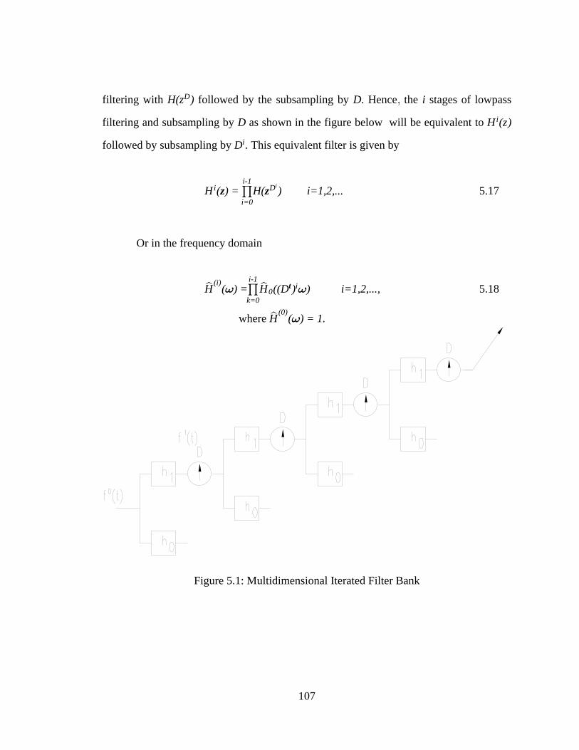
107

filtering with followed by the subsampling by . Hence the stages of lowpassH(z ) D iD ß

filtering and subsampling by as shown in the figure below will be equivalent to D H (z)i

followed by subsampling by This equivalent filter is given byD .i

5.17H ( ) = H( ) i=1,2,...i D

i=0

i-1z z# i

Or in the frequency domain

5.18H ( ) = H ((D ) ) i=1,2,...,s s(i)

k=0

i-10

i= =# t

where H ( ) = 1.s (0)=

Figure 5.1: Multidimensional Iterated Filter Bank

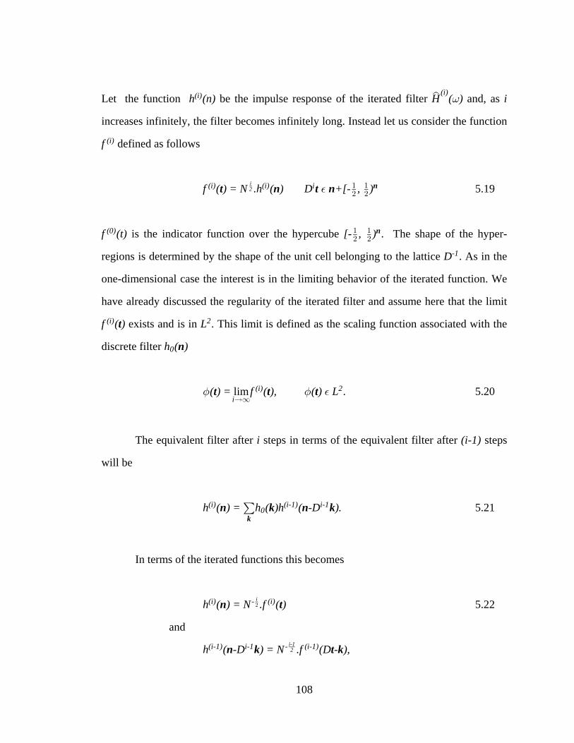
108

Let the function be the impulse response of the iterated filter and, as h (n) H ( ) i(i) (i)s =

increases infinitely, the filter becomes infinitely long. Instead let us consider the function

f (i) defined as follows

5.19f ( ) = N .h ( ) D +[- , )(i) (i) it n t ni2 % " "

# #n

f (t) [- , )(0) is the indicator function over the hypercube . The shape of the hyper-" "# #

n

regions is determined by the shape of the unit cell belonging to the lattice . As in theD-1

one-dimensional case the interest is in the limiting behavior of the iterated function. We

have already discussed the regularity of the iterated filter and assume here that the limit

f ( ) L(i) 2t exists and is in . This limit is defined as the scaling function associated with the

discrete filter h ( )0 n

. 5.209 9 %( ) = f ( ), ( ) Lt t tlimi

(i) 2Ä∞

The equivalent filter after steps in terms of the equivalent filter after stepsi (i-1)

will be

5.21h ( ) = h ( )h ( -D ).(i) (i-1) i-10n k n k

k

In terms of the iterated functions this becomes

5.22h ( ) = N .f ( )(i) - (i)n ti#

and

h ( -D ) = N .f (D - ),(i-1) i-1 - (i-1)n k t ki-12

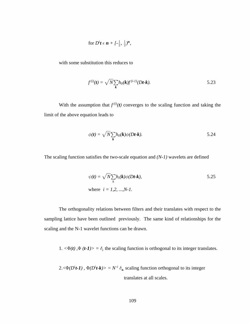
109

for , D + [- , )it n % " "# #

n

with some substitution this reduces to

5.23f ( ) = N h ( )f (D - ).(i) (i-1)0t k t kÈ

k

With the assumption that converges to the scaling function and taking thef ( )(i) t

limit of the above equation leads to

5.249 9( ) = N h ( ) (D - ).t k t kÈk

0

The scaling function satisfies the two-scale equation and wavelets are defined(N-1)

5.25< 9( ) = N h ( ) (D - ),t k t kÈk

i

where i = 1,2, ...,N-1.

The orthogonality relations between filters and their translates with respect to the

sampling lattice have been outlined previously. The same kind of relationships for the

scaling and the N-1 wavelet functions can be drawn.

1. the scaling function is orthogonal to its integer translates. < ( ) , ( - )> = F F $t t 1 l

2. scaling function orthogonal to its integer< (D ) , (D - )> = N F F $i i -it-1 t k lk

translates at all scales.

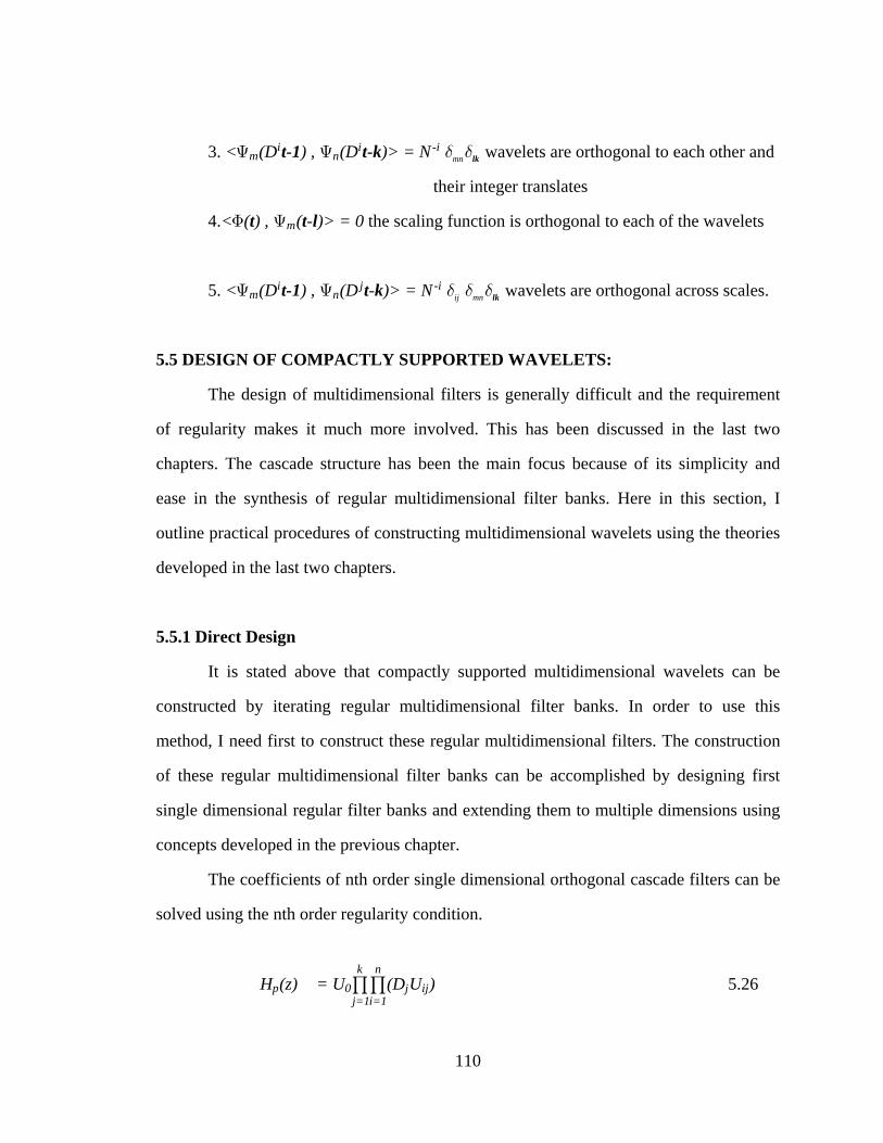
110

3. wavelets are orthogonal to each other and< (D ) , (D - )> = N G G $ $m ni i -it-1 t k mn lk

their integer translates

4. the scaling function is orthogonal to each of the wavelets< ( ) , ( - )> = 0F Gt t lm

5. wavelets are orthogonal across scales.< (D ) , (D - )> = N G G $ $ $m ni j -it-1 t k ij mn lk

5.5 DESIGN OF COMPACTLY SUPPORTED WAVELETS:

The design of multidimensional filters is generally difficult and the requirement

of regularity makes it much more involved. This has been discussed in the last two

chapters. The cascade structure has been the main focus because of its simplicity and

ease in the synthesis of regular multidimensional filter banks. Here in this section, I

outline practical procedures of constructing multidimensional wavelets using the theories

developed in the last two chapters.

5.5.1 Direct Design

It is stated above that compactly supported multidimensional wavelets can be

constructed by iterating regular multidimensional filter banks. In order to use this

method, I need first to construct these regular multidimensional filters. The construction

of these regular multidimensional filter banks can be accomplished by designing first

single dimensional regular filter banks and extending them to multiple dimensions using

concepts developed in the previous chapter.

The coefficients of nth order single dimensional orthogonal cascade filters can be

solved using the nth order regularity condition.

5.26H (z) = U (D U )p 0 j ijj=1i=1

k n##

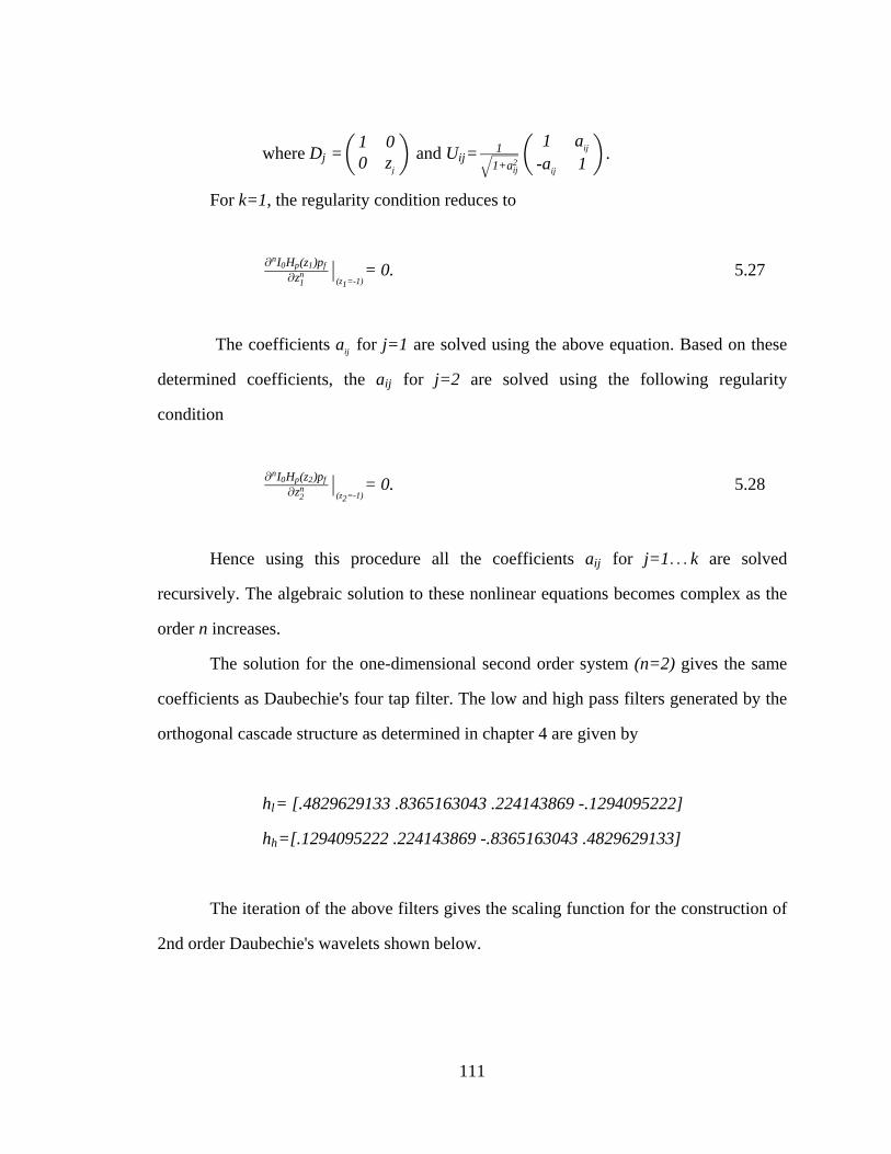
111

where and .D = U =1 00 z

1 a-a 1j ij

11+aŒ Œ

j ij2

ij

ijÉ For , the regularity condition reduces to k=1

5.27``

n0 p 1 f

n1 (z =-1)1

I H (z )pz

¸ = 0.

The coefficients for are solved using the above equation. Based on thesea j=1ij

determined coefficients, the for are solved using the following regularitya j=2ij

condition

5.28``

n0 p 2 f

n2 (z =-1)2

I H (z )pz

¸ = 0.

Hence using this procedure all the coefficients for are solveda j=1 kij á

recursively. The algebraic solution to these nonlinear equations becomes complex as the

order increases.n

The solution for the one-dimensional second order system gives the same(n=2)

coefficients as Daubechie's four tap filter. The low and high pass filters generated by the

orthogonal cascade structure as determined in chapter 4 are given by

h = [.4829629133 .8365163043 .224143869 -.1294095222]l

h =[.1294095222 .224143869 -.8365163043 .4829629133]h

The iteration of the above filters gives the scaling function for the construction of

2nd order Daubechie's wavelets shown below.

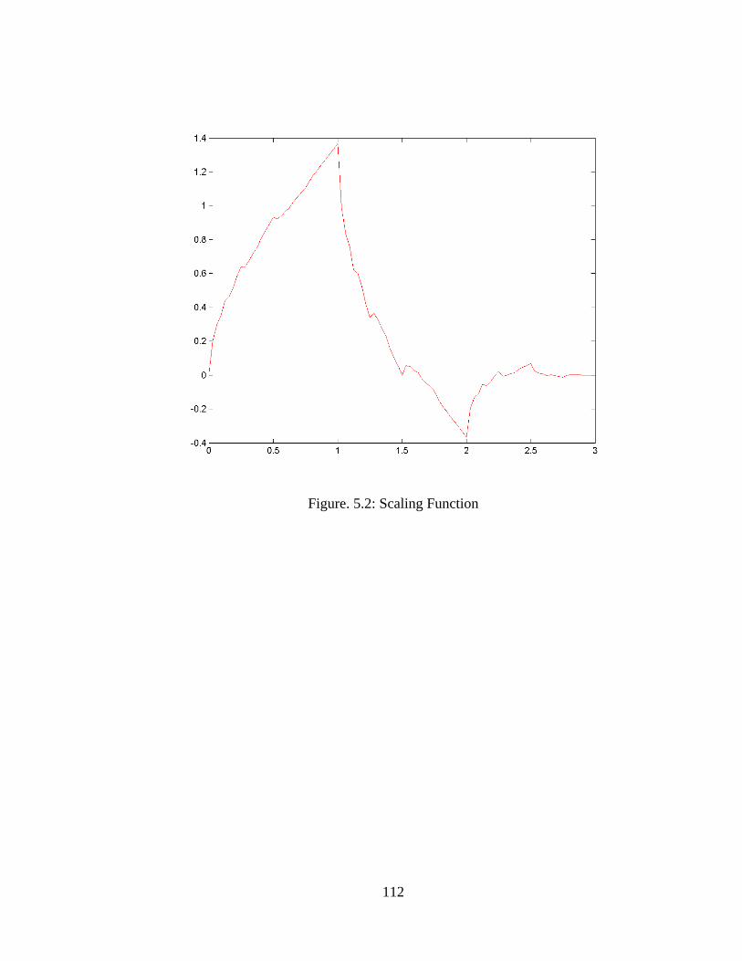
112

Figure. 5.2: Scaling Function

113

Figure. 5.3: Daubechie's Wavelet

The same methods developed in Chapters 3 and 4 are used to determine the

higher-dimensional filter coefficients. The 2nd-order two-dimensional filter coefficients

are given by

h = 0 .1120719339 -.1941142837 0

.2414814568 -.4182581524 -.1120719339 -.064704761200 .7244443705 .4182581522 0

lÔ ×Õ Ø

h = 0 -.4182581522 .7244443705 0

.06470476120 -.1120719339 .4182581524 .24148145680 .1941142837 .1120719339 0

hÔ ×Õ Ø

114

The 2nd order two dimensional wavelet is constructed using the scaling function

obtained by iterating the above filters. The scaling and wavelet functions are shown in

the Figure below.

Figure. 5.4: 2-D Scaling function

115

Figure. 5.5: 2-D Wavelet function

Again the same concepts are used to construct the three dimensional filters. These

three dimensional filters are iterated to give the 2nd-order, three-dimensional scaling and

wavelet functions.

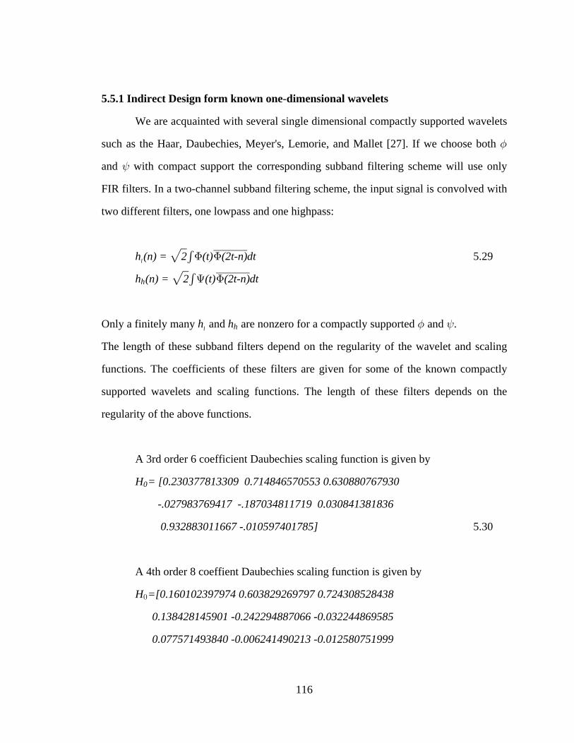
116

5.5.1 Indirect Design form known one-dimensional wavelets

We are acquainted with several single dimensional compactly supported wavelets

such as the Haar, Daubechies, Meyer's, Lemorie, and Mallet [27]. If we choose both 9

and with compact support the corresponding subband filtering scheme will use only<

FIR filters. In a two-channel subband filtering scheme, the input signal is convolved with

two different filters, one lowpass and one highpass:

5.29h (n) = 2 (t) (2t-n)dt lÈ 'F F

h (n) = 2 (t) (2t-n)dth È 'G F

Only a finitely many and are nonzero for a compactly supported and .h hl h 9 <

The length of these subband filters depend on the regularity of the wavelet and scaling

functions. The coefficients of these filters are given for some of the known compactly

supported wavelets and scaling functions. The length of these filters depends on the

regularity of the above functions.

A 3rd order 6 coefficient Daubechies scaling function is given by

H = [0.230377813309 0.714846570553 0.6308807679300

-.027983769417 -.187034811719 0.030841381836

0.932883011667 -.010597401785] 5.30

A 4th order 8 coeffient Daubechies scaling function is given by

H =[0.160102397974 0.603829269797 0.724308528438!

0.138428145901 -0.242294887066 -0.032244869585

0.077571493840 -0.006241490213 -0.012580751999

117

0.003335725285] 5.31

A th order 23 coefficient symmetric Mallat scaling functionn

H = [-.002 -.003 .006 .006 -.013 .012 -.030 0.023 -.0780

-.035 .307 0.542 0.307 -.035 -.078 .023 -.030 .012

-.013 .006 .006 -.003 -.002] 5.32

The polyphase matrices for the above scaling functions can be reconstructed

using the filter coefficients and the forward polyphase vector for a given sampling

density. Based on these polyphase matrices cascade representations can also be

formulated. Once these single dimensional cascade representation are drawn the

multidimensional filter banks with the same order of regularity are constructed using

some of the methods discussed in the previous chapters. For the two-channel case the

relation between the low and high-pass filter and the polyphase matrix can be written as

5.33H(z) = = H (z )p (z) h (z)h (z)” •l

fh

pD

This polyphase matrix can be written in cascade form as follows

5.34H (z) = U D U p 0 i ii=1

n# = Œ Œ Œ#1 a 1 0 1 a

-a 1 0 z -a 10 i

0 ii=1

n

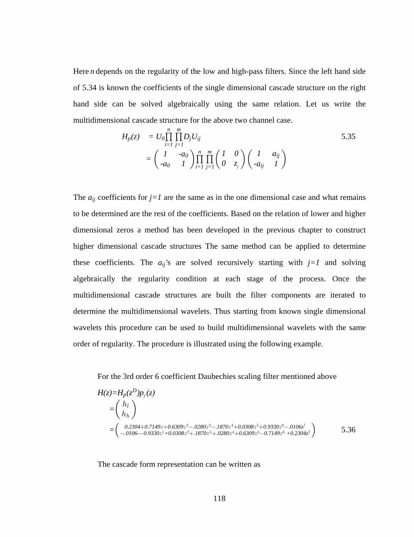
118

Here depends on the regularity of the low and high-pass filters. Since the left hand siden

of 5.34 is known the coefficients of the single dimensional cascade structure on the right

hand side can be solved algebraically using the same relation. Let us write the

multidimensional cascade structure for the above two channel case.

5.35H (z) = U D Up 0 j iji=1 j=1

n m# # = Œ Œ Œ# #1 -a

-a 1 -a 1 1 00 z

1 a0

0 iji=1 j=1

n m ij

j

The coefficients for are the same as in the one dimensional case and what remainsa j=1ij

to be determined are the rest of the coefficients. Based on the relation of lower and higher

dimensional zeros a method has been developed in the previous chapter to construct

higher dimensional cascade structures The same method can be applied to determine

these coefficients. The s are solved recursively starting with and solvinga ' j=1ij

algebraically the regularity condition at each stage of the process. Once the

multidimensional cascade structures are built the filter components are iterated to

determine the multidimensional wavelets. Thus starting from known single dimensional

wavelets this procedure can be used to build multidimensional wavelets with the same

order of regularity. The procedure is illustrated using the following example.

For the 3rd order 6 coefficient Daubechies scaling filter mentioned above

H(z)=H (z )p (z)pD

f

=Π22

6

2

=Š ‹0.2304 0.7149 0.6309 .0280 .1870 0.0308 0.9330 .0106z.0106- 0.9330 +0.0308 .1870 .0280 0.6309 0.

D D D D D D D D D D D

# $ % & ' (

" # $ % & 7149 +0.2304zD' ( 5.36

The cascade form representation can be written as

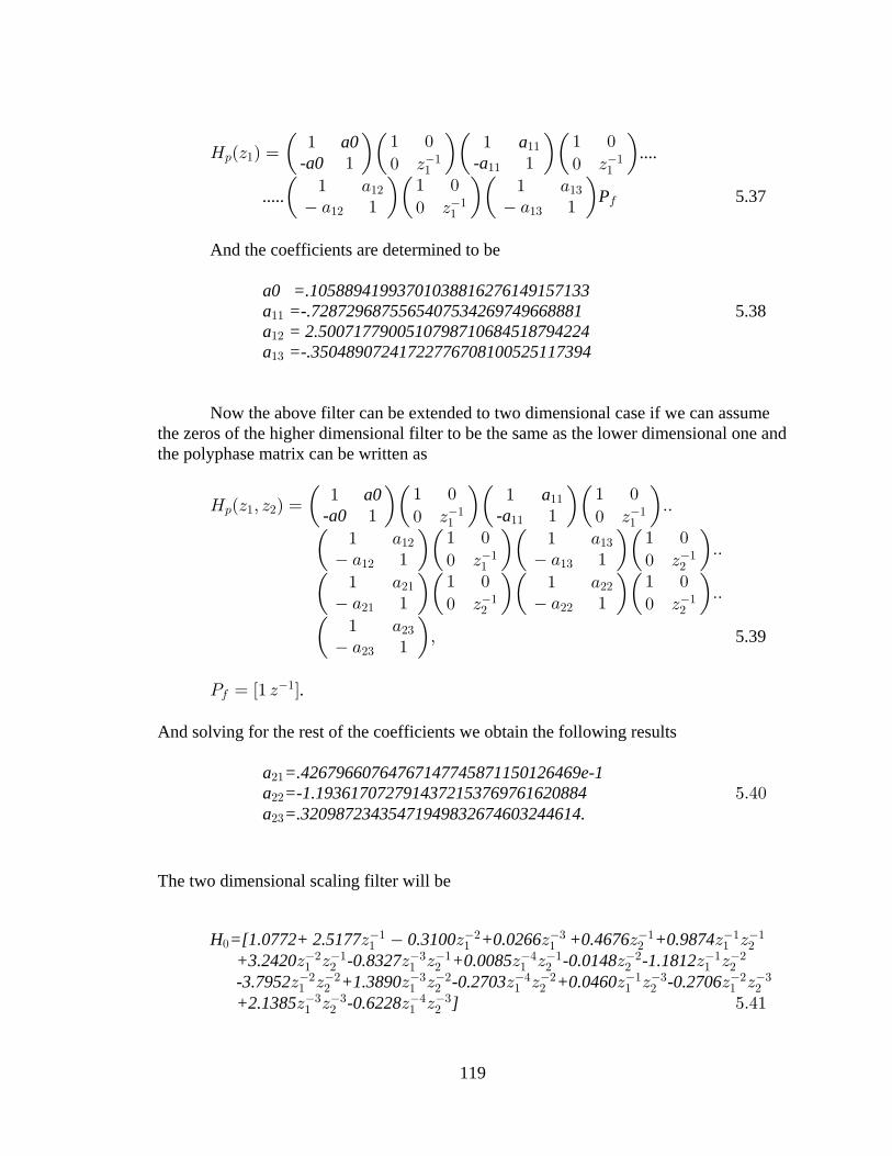
119

L ÐD Ñ œ" "

" "" ! " !

! D ! D: " " "" "

""

""Œ Œ Œ Œa0 a

-a0 -a ....

5.37..... PŒ Œ Œ" + " + + " + "

" !

! D"# "$

"# "$""

0

And the coefficients are determined to be

a0 =.10588941993701038816276149157133 5.38 a =-.7287296875565407534269749668881""

a = 2.5007177900510798710684518794224"#

a =-.35048907241722776708100525117394"$

Now the above filter can be extended to two dimensional case if we can assumethe zeros of the higher dimensional filter to be the same as the lower dimensional one andthe polyphase matrix can be written as

L ÐD ß D Ñ œ ÞÞ" "

" "" ! " !

! D ! D: " # " "" "

""

""Œ Œ Œ Œa0 a

-a0 -a

Œ Œ Œ Œ" + " + + " + "

" ! " !

! D ! DÞÞ"# "$

"# "$" "" #

Œ Œ Œ Œ" + " + + " + "

" ! " !

! D ! DÞÞ#" ##

#" ##" "# #

5.39Π" + + "

ß#$

#$

T œ Ò" D Ó0" .

And solving for the rest of the coefficients we obtain the following results a =.42679660764767147745871150126469e-1#"

a =-1.1936170727914372153769761620884## &Þ%! a =.32098723435471949832674603244614.#$

The two dimensional scaling filter will be

H =[1.0772+ 2.5177 0.3100 +0.0266 +0.4676 +0.9874!" # $ " " "" " # " #"D D D D D D

+3.2420 -0.8327 +0.0085 -0.0148 -1.1812D D D D D D D D D# " $ " % " # " #" # # " # # " #"

-3.7952 +1.3890 -0.2703 +0.0460 -0.2706D D D D D D D D D D# # $ # % # " $ # $" # # " # " "" # #

+2.1385 -0.6228 ]D D D D$ $ % $" # #" &Þ%"

120

h = .-0.2703 1.3890 -3.79526

Î ÑÐ ÓÐ ÓÏ Ò

! Þ!#'' Þ$"!! #Þ&"(( "Þ!((#Þ!!)& !Þ)$#( $Þ#%#! !Þ*)(% Þ%'('

"Þ")"# !Þ!"%) !Þ'##) #Þ"$)& Þ#(!' !Þ!%' !

SUMMARY:

In this chapter practical procedures for the construction of compactly supported

multidimensional wavelets have been outlined. These procedures have been illustrated

using practical examples. The relation of zeros between higher and lower dimensional

filters have been the key factor for setting these procedures. The multidimensional

nonseparable wavelets constructed using iteration of multidimensional filters will be

utilized in the reconstruction and denoising of multidimensional images in the next

chapter.

121

CHAPTER 6

APPLICATIONS:IMAGE RESTORATION

6.1 INTRODUCTION

The focus of all previous chapters have been first to construct regular

multidimensional nonseparable filter banks and then iterate these filters to construct a

compactly supported nonseparable multidimensional wavelets. In the this chapter, I will

discuss the application of these multidimensional nonseparable wavelets in

multidimensional image processing. Typical goals in image processing include

restoration, enhancement, smoothing/extrapolation, synthesis, detection/estimation and

spectral factorization [32]. In this chapter, I consider the problem of image restoration in

multiple dimensions. The use of wavelet for the task of image restoration and

enhancement is relatively new and rapidly emerging concept in image processing.

Wavelet methods for de-noising and de-blurring have attracted considerable interest

especially in the fields of medical imaging, synthetic aperture radar, extra galactic

astronomy, computer vision, molecular spectroscopy and others. The main focus of this

chapter is to test and demonstrate the application of the multidimensional nonseparable

filterbanks constructed in the previous chapters in the restoration and reconstruction of

images.

6.2 PRELIMINARIES

The field of image restoration began several decades ago when scientists were

involved in the space programs that produced incredible images of the Earth and our

122

Solar system [67], [46]. The images obtained from the various planetary missions of the

time were subject to many photographic degradation's as a result of substandard imaging

environment, vibration in machinery and the spinning and tumbling of the spacecraft.

The degradation of images was not a small problem, considering the enormous expense

required to obtain these images. Thus the need to develop methods for the retrieval of

meaningful information from degraded images became critical. To this end inordinate

amount of effort has been put to develop techniques for the restoration of images in the

last few decades. As a result some of the most common algorithms in one-dimensional

signal processing and estimation theory found their way into the realm of image

restoration. A lot of the work done in image processing have their primary roots in

classical signal processing approaches to estimation theory, filtering, and numerical

analysis.

The wide areas of application of image processing has contributed to the diverse

perspectives in the development of the theory. Astronomical imaging is still one of the

primary applications of digital image restoration. Extraterrestrial observations of the

Earth and the planets were degraded by motion of blur as a result of slow camera shutter

speeds relative to rapid spacecraft motion. Images obtained were often subject to noise of

one form or another. Often astronomical imaging degradation problems are characterized

by Poisson noise which is signal-dependent and has its roots in the photon-counting

statistics involved with low light sources. Another type of noise found in these images is

Gaussian noise, which often arises from electronic components in the imaging system

and broadcast transmission effects.

In the areas of medical imaging, image restoration has played an important role.

Restoration has been used for filtering of Poisson distributed film grains noise in chest X-

rays, mammogram's, digital angiographic images and the removal of additive noise in

123

Magnetic Resonance Imaging (MRI) [30]. Another emerging application of image

restoration in medicine is in the areas of quantitative autoradiology (QAR).

Image restoration has also wide application in the media and particularly in the

movies industry. Image restoration techniques are used for the restoration of blurry, aged

Polaroid negative images of the last decade. Image restoration is used not only to restore

aged and deteriorated films it is also used to colorize black-and-white films.

In general there are significant works done in the areas of image restoration in

several application areas. Image restoration has been applied in law enforcement and

forensic science for an number of years. The restoration of blurry photographs of license

plates and crime scenes and poor-quality security videotapes is frequent. Another

exciting application of image restoration is in the field of image and video coding.

Several techniques are being developed to improve coding efficiency, and reduce bit

rates of coded images.

Image restoration is being used in many other applications as well. A few of them

include restoration of blurry X-ray images of aircraft wings to improve federal aviation

inspection procedures, for printing of high quality continuous images, in assembly line

manufacturing of electronic parts and in defense applications such as guided missiles

which may obtain distorted images due to the effect of pressure differences around the

camera mounted on the missile. Image restoration plays a significant role in today's

world.

6.3 IMAGE RESTORATION AND RECONSTRUCTION

Image restoration is a field that studies methods used to recover an original scene

from degraded observations. Techniques used for image restoration are oriented toward

modeling the degradation's, usually blur and noise, and applying an inverse procedure to

124

obtain an approximation of the original scene. Reconstruction are generally separate from

image restoration since they operate on a set of image projections and not on a full image.

However, restoration and reconstruction techniques do share the same objective of

recovering the original image and end up solving the same mathematical problem.

Developing techniques to perform the image restoration task requires the use of

models not only for the degradation's, but also for the images themselves. Here we will

be concerned with some of the well developed techniques. A more general and

comprehensive degradation and restoration model is shown in the Figure 6.1 below.

Figure 6.1: Image Degradation Module and Restoration Process

It is evident from this figure that the amount of prior knowledge plays a major

part in achieving the best restorations. These are knowledge of degradation, knowledge

about the original image and prior knowledge of , i.e. blur identification.L

125

6.3.1 SOURCE OF IMAGE DEGRADATION

The general discrete model for a linear degradation caused by blurring and

additive noise can be given by the following superposition summation

= 6.1CÐ Ñ 2Рч0Ð Ñ 8Ð Ñ8 8 8 8

= O

5 5 82Ð8 Ñ0Ð Ñ8Ð Ñ

where represents the original image0Ð Ñ8

is the degraded imageCÐ Ñ8

represents an additive noise introduced by the8Ð Ñ8

system usually taken as zero mean Gaussian

distributed noise term.

and

* indicates -dimensional convolution8

The blurring process described by equation 6.1 is linear. Often the linear

convolution is approximated by circular convolution. This involves treating the image as

one period from the -dimensional periodic signal. The borders of an image are often8

treated as symmetric extensions of the image. Such approaches seek to minimize the

distortion at the borders caused by filtering algorithms which must perform

deconvolution over the entire image. When implementing image restoration algorithms, it

is very important to consider how the borders of the image are treated, as different

approaches can result in very different restored images. The several analytical models are

frequently used in equation to represent the shift-invariant image degradation. The

models are developed for varied blurs such as motion blur, turbulence blur, etc andÞ

additive noise such as Gaussian and Poisson.

126

6.3.2 SOME CLASSICAL IMAGE RESTORATION TECHNIQUES

One of the many common approaches to image restoration and solving equation

6.1 is the minimum mean square error (MSE) an optimization based on varied criteria

such as BSNR (Blurred Signal-to-Noise Ratio), ISNR (Improvement to Signal-to-Noise

Ratio). Even though these criteria do not always reflect the perceptual properties of the

human visual system, they serve to provide an objective standard by which to compare

different techniquesÞ

Another is the classical direct approach to solving equation 6.1 i.e. finding an

estimate of which minimizes the norm0s

mC L0ms# 6.2

Thus providing a least squares fit to the data. This leads to the generalized

inverse filter, which is given by the solution

6.3ÐL LÑ0 œ L CsX X

An alternative approach to solving equation 6.1. in a regularized fashion can lead

to direct restoration approaches when considering either a stochastic or a deterministic

model for the original image . In both cases, the model represents prior information0

about the solution which can be used to make the problem well-posed.

Another approach is the iterative image restoration algorithms. The primary

advantages of iterative techniques are that there is no need to explicitly implement the

inverse operator and that the process may be monitored as it progresses. Iterative

127

algorithms are very well suited to restoring images suffering from a variety of

degradation's, such as linear, nonlinear, spatially varying, or spatially invariant blurs, and

signal-dependent noise, because of the flexible framework provided by each approach.

One of the most basic deterministic iterative techniques considers solving

6.4ÐL L G GÑ0X Xα

with the method of successive approximations. This leads to the following iteration for 0

6.50 œ L C!X"

6.60 œ 0 ÒL C ÐL L G GÑ0 Ó5" 5 5

X X X" α

This iteration converges if

where is the largest eigenvalue of the! 7+B" -#l 7+Bl-

matrix ÐL L G GÑÞX Xα

6.3.3 WAVELETS AND IMAGE RESTORATION

In the last two decades, there has been considerable interest in the use of wavelet

transforms for image restoration, reconstruction, feature extraction anedge detection [3],

[43]. One method applied by R.R. Coifman [17] and D. L. Donoho [23] has been to use

the transform-based thresholding defined below

Transform the noisy data into an orthogonal domain

Apply soft or hard thresholding to the resulting coefficients, thereby suppressing

those coefficients smaller than a certain amplitude.

Transform back into the original domain.

128

The denoising algorithm developed by Mallat et al. which is a wavelet based

technique has been developed and refined since it first came out. One of our motivation

in this chapter is to test some of these algorithms for multidimensional image processing.

Figure 6.2. shows a basic model of an image restoration system. In the system

module, is the original signal that is degraded by the linear operation ofBÐ3ß 4ß 5Ñ $H

0Ð3ß 4ß 5Ñ 8Ð3ß 4ß 5Ñ $H .Ð3ß 4ß 5Ñ and the addition of the noise to form the degraded signal .

The restoration filter is which is convolved with the degraded signal1Ð3ß 4ß 5Ñ $H

.Ð3ß 4ß 5Ñ $H CÐ3ß 4ß 5Ñ to form the restored signal . The additive noise is modeled as a

Gaussian process (White noise).

Figure 6.2: Basic Image Resolution Module

In the denoising algorithm, the separation of the signal information from the noise

is done by discriminating the signal singularities from the noise singularities. This is done

129

by analyzing the behavior of the wavelet transform maxima across scales [24], [44, [89].

Advantage is taken of the spatial coherence of the signal singular structures to suppress

the noise components.

Once the signals have been decomposed into elementary building blocks that are

well localized both in space and frequency, the local regularity of the signals can then be

characterized by the wavelet transform. The wavelet's modulus maxima across scales are

analyzed. Noise fluctuations that dominate the signal singularities are then removed. The

remaining local maxima positions and amplitudes are modified, and the "denoised" signal

is finally reconstructed from these modulus maxima.

The denoising algorithm consists of three different stages, suppressing the noise

components, enhancing the signal components and then reconstructing the "denoised"

signal from the remaining local maxima.

6.4 SIMULATION

In this section several simulations have been made to show the implementation of

separable and nonseparable multidimensional filterbanks constructed in the previous

chapters for image reconstruction. The solution to the filter coefficients has been worked

out using Maple 7 [88] and all the simulations have been done using matlab[55]. Several

algorithms have been developed to accommodate the multidimensional nonseparable

sampling and convolution operations. All of the images used in the simulation and the

denoising algorithms used here are obtained and adopted from Mathlab and Wavelab [75]

except for the nonseparable cases. The improvement in image restoration as a result of

higher order filters is demonstrated. Some of the image libraries in image processing

toolbox of matlab are used to demonstrate the results.

130

6.4.1 IMAGE RECONSTRUCTION

6.4.1.1 2-D IMAGES.

Using the methods developed in the previous chapters a 2-D nonseparable filter is

designed from a 1-D filter with 2-order regularity. Figure 6.2 shows a first level image

reconstruction using the 2nd order 2-D nonseparable filterbank. Higher levels of image

reconstruction can be built based on the same concepts and algorithms developed for the

first level.

Figure. 6.3: Image Reconstruction 2nd Order Nonseparable Process

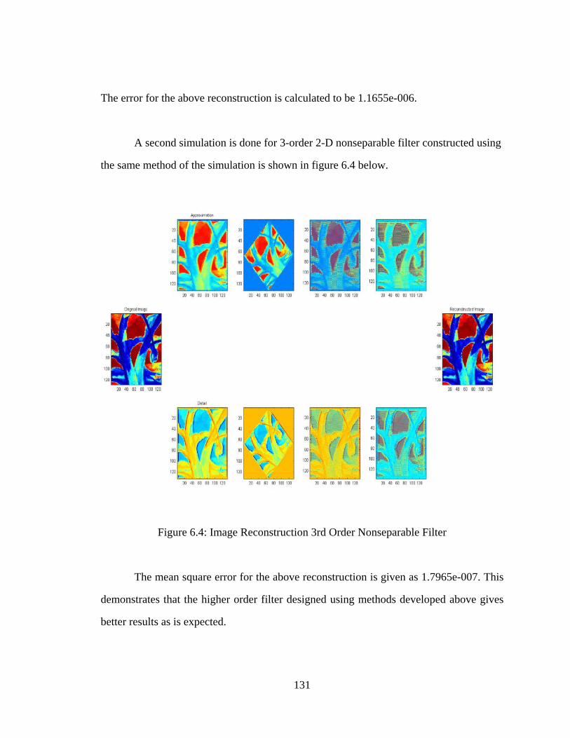
131

The error for the above reconstruction is calculated to be 1.1655e-006.

A second simulation is done for 3-order 2-D nonseparable filter constructed using

the same method of the simulation is shown in figure 6.4 below.

Figure 6.4: Image Reconstruction 3rd Order Nonseparable Filter

The mean square error for the above reconstruction is given as 1.7965e-007. This

demonstrates that the higher order filter designed using methods developed above gives

better results as is expected.

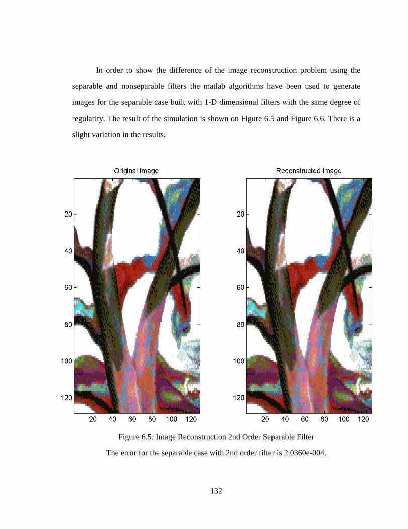
132

In order to show the difference of the image reconstruction problem using the

separable and nonseparable filters the matlab algorithms have been used to generate

images for the separable case built with 1-D dimensional filters with the same degree of

regularity. The result of the simulation is shown on Figure 6.5 and Figure 6.6. There is a

slight variation in the results.

Figure 6.5: Image Reconstruction 2nd Order Separable Filter

The error for the separable case with 2nd order filter is 2.0360e-004.

133

Figure 6.6: Image Reconstruction 3rd Order Separable Filter

The error for the separable case with 3rd order filter is 3.000e-005.

6.4.1.2 3-D Image

The higher order filter designed using the methods developed in the previous

chapters have been used to reconstruct 3-D images using the separable method. The

results of the simulation is shown in Figures 6.7 and 6.8. However, the nonseparable

134

construction is not shown because of computational and programming complexity of the

3-D nonseparable sampling and convolution.

Figure 6.7: Original 3D Flow

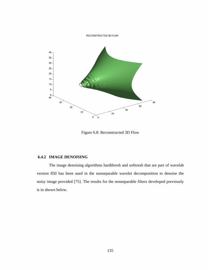
135

Figure 6.8: Reconstructed 3D Flow

6.4.2 IMAGE DENOISING

The image denoising algorithms hardthresh and softtresh that are part of wavelab

version 850 has been used in the nonseparable wavelet decomposition to denoise the

noisy image provided [75]. The results for the nonseparable filters developed previously

is in shown below.

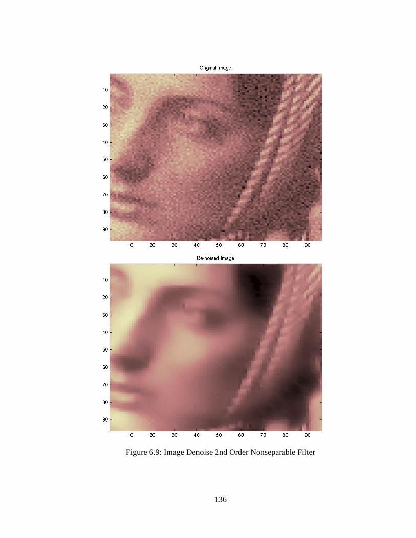
136

Figure 6.9: Image Denoise 2nd Order Nonseparable Filter

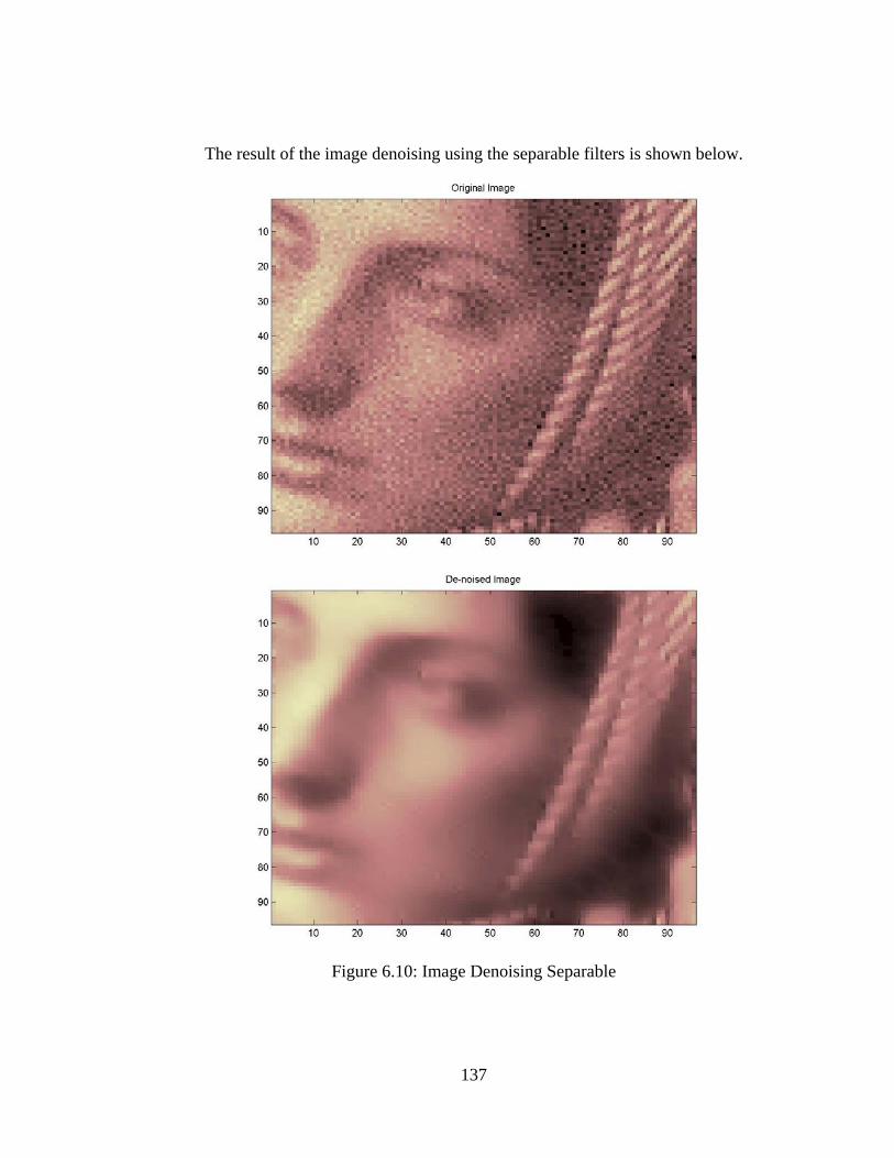
137

The result of the image denoising using the separable filters is shown below.

Figure 6.10: Image Denoising Separable

138

6.6 SUMMARY

In this chapter the multidimensional nonseparable as well as separable filters

constructed using methods developed in the previous chapters have been applied for the

reconstruction and denoising of images. The results demonstrate that the filters

constructed using the methods developed in this dissertation accomplish the desired

results as illustrated by the different examples. Higher order filters produce better results

than lower order filters. The nonseparable filters with isotropic sampling matrices also

give better results compared to the separable filters.

139

CHAPTER 7

CONCLUSION AND DIRECTIONS

7.1 CONTRIBUTION

In this dissertation multidimensional multirate system theory and applications

have been studied. The basic concepts of wavelet analysis, multirate filter banks and

multiresolution analysis are summarized. The interrelationship of these concepts and the

development of a unified approach in single dimension is outlined. The extension of

these concepts to multiple dimensions based on multidimensional sampling and lattice

structures has been described. The construction of continuous wavelets from iterated

filterbanks depends on the construction of regular filterbanks be it in single or multiple

dimensions. This dissertation investigates the conditions of regularity in the

multidimensional case and proposes new method for the construction of

multidimensional filters for wavelet transforms satisfying constraints of regularity and

vanishing moments [76].

In this dissertation the existence of the relations of zeros in the lower and higher

dimensional filterbanks are proved for a class of filters with cascade structures. This

relation has been first observed but not established by J. Kovacevic and M. Vetterli [39].

Proving this relationship is fundamental for the transformation of a one-dimensional into

a two-dimensional into a three-dimensional regular filters. In this dissertation two

different approaches has been used to establish this relation. First, basic theorems of

linear spaces have been used to show the existence of the relation of zeros of higher and

140

lower dimensional regular filters with cascade structures. Second, theories and concepts

of polynomial matrix description are used to prove the same relation.

Based on the above established relation this dissertation develops methods and

procedures for the construction of regular nonseparable multidimensional filters. The -8

dimensional nonseparable regular filter is constructed using -dimensional regularÐ8 "Ñ

filter. And by extension the -dimensional nonseparable regular filter is constructed8

using single dimensional regular filters. Based on this relation practical procedures for

the recursive construction of regular multidimensional filterbanks and compactly

supported multidimensional wavelets has been developed. The above stated relation has

been exploited to construct higher dimensional filters banks from known lower

dimensional filterbanks with varied degrees of regularity. These filterbanks with non-

diagonal sampling lattice are iterated to construct multidimensional nonseparable wavelet

basis. The method substantially reduces the computational complexity of constructing the

multidimensional filters. The filter coefficients are calculated at each stage of the

recursive processes thereby reducing the number of undetermined coefficient and making

the algebraic equation much more manageable. The arithmetic operation grows linearly

with the order of regularity instead of where is the determinant ofSÐR Ñ SÐR Ñ Hk kH k kthe dilation matrix. Besides, single dimensional filters with proven characteristics and

regularity could be easily transformed to multiple dimensions.

In the dissertation several examples have been used to illustrate the concept and

construct multidimensional filterbanks starting from known one-dimensional scaling

filters with varied degree of regularity. The iteration of these filters gives nonseparable

wavelets depending on the lattice structure. The single dimensional second and third

order Daubehcies scaling filters are used to construct 2-D and 3-D nonseparable

multidimensional wavelet basis. The results obtained agree with published values.

141

Finally the multidimensional nonseparable wavelets constructed above are used in

the reconstruction and denoising of multidimensional images. However, the choice of the

dilation matrix that determines the downsampling and upsampling is very important in

the image processing [9]. The dilation matrix determines all aspects of the filter design as

well as the visual effect. This matrix has to be isotropic to ensure no distortion in image

processing. The multidimensional filters with isotropic matrices are employed for the

reconstruction and denoising of multidimensional images. The performance of the

separable and nonseparable filters with second and third order regularity are compared.

Finally a simulation has been done and the results of 2-D images are plotted. The 2-D

nonseparable filters constructed with quincunx dilation matrix with equal singular values

show no distortions. The calculated errors for the nonseparable filters show improvement

over those obtained by separable filters. However, not all dilation matrices and their

corresponding nonseparable filterbanks give better results unless the matrices are

isotropic. The selection of the dilation matrices requires the satisfaction of additional

constraint.

7.2 FUTURE RESEARCH

The design of filter banks based on factorization of polyphase matrices is

challenging because of the large number of parameters to be determined. The number is

attenuated by imposing linear phase perfect reconstruction and critical sampling

constraints. The results are also limited to real valued coefficients. Yet the extension of

the results in this dissertation to higher dimensions has been computationally

cumbersome and even if the 3-D nonseparable filterbanks are constructed applying them

to image reconstruction and denoising requires additional work in 3-D convolution and

programming.. The effect of relaxation of the constraints such as oversampling and

142

concatenation of filters with varied features need further research [50], [94]. The choice

of dilation (downsampling and upsampling) matrix for optimal filter design and image

processing needs to be further investigated. Generating integer valued dilation matrix that

are critically sampled and satisfying the isotropic condition is a real challenge [68], [86].

For example, the FCO used to construct 3-D nonseparable filterbank is not isotropic and

is liable to image distortions. Despite the last twenty years of research in the wavelet

transforms and the continually increasing areas of applications there are several areas that

need further research more so in the area of multidimensional nonseparable wavelet

construction [19], [60], [62].

143

APPENDIX A:REISZ BASIS

A function is said to generate a Reisz basis( or unconditional basis)G % L (R)2

{ } Gb,j,k with the sampling rate b if both the following properties are satisfied.0

1) The linear span is dense in < j,k Z > L (R)G %b,j,k2

2) There exists positive constant A, B with 0<A<B< such that∞

A.1A C C B Cm m Ÿ m m Ÿ m mj,k j,k b ,j,k j,klj,k Z

l22 2

0 l22

%

G 2

for all {C l (Z )j,k%2 2

If generates Riesz basis with then is called R-function. If is an -G G Gb =1 R0

function then there is a unique Riesz basis which is dual to in the{ } of L (R) { }G Gj,k 2

j,k

sense

A.2< , > = j,k,l,m Z G G $ $ %j,k j,l k,ml,m

Hence every function has a unique series expansionf L (R)% 2

A.3f(x) = < f, > (x)j,k=-

j,k∞

G Gj,k

Although the coefficients are the values of the wavelet transform of f relative to

G the series is not necessarily a wavelet series. To qualify as a wavelet series there must

exit some such that the dual basis is obtained form by L (R) { } ~ ~G % G G2 j,k

A.4 (x) = (x) ~G G

j,kj,k

(x) = 2 (2 -k) ~G Gj,k

jx"#

If is orthonormal basis of then or . In general { } L (R) = = ~ ~G G G G G Gj,k j,k

2 j,k

does not exit. If is chosen such that it exists then can be recovered from the pair G Gf { ,

G~} by

144

A.5f(x) = <f , > (x)~G Gj,k j,k

= <f , > (x)~G Gj,k j,k

145

APPENDIX: B

NOTATION AND DEFINITIONS

This section contains most of the definitions involving multidimensional z-transform

and sampling.

1. Multidimensional z-Transform

1.1 Raising an n-dimensional complex vector to an n-dimensional z =(z ,z ....z )1 2 n

integer vector k =(k ,k ....k )1 2 n

B.1zk = z z ...z 1 2k k

nk1 2 n

1.2 Raising a to a matrix power D denotesz

B.2zD1 2 n = (z , z ,...z ) d d d1 2 n

where is the column of the matrix .di D

1.3 The equivalent Nth root of unityis defined as

B.3W ( ) = (e ,.....e ) D-j< , > -j< , >= = =d d1 n

1.4 The z-transform of a discrete sequence is defined asx( )=h(k ,k ....k )k 1 2 n

x( ) = x( )z k zk

k

% m

-n

B.4 = ..... x(n ,...n )z ....z n n

1 N 1-n

N-n

1 N

1 N

2. Multidimensional Fourier transform

146

The Fourier transform of the multidimensional function x is given by

B.5x( ) = x( )e =k

k

-j< , >

% mnk =

3. Lattice:

Lattice : is the set of all linear combinations of basis vectors N = (n ,n ....n )n 1 2 N

with integer coefficients.

Sublattice: If every point of the lattice is also a point of the lattice M then isA A

sublattice of . The determinant of is an integer multiple of theM A

determinant of . M

Greatest Common Sublattice(gcs : is the set of all points belonging to both( , )A A1 2

and .A A1 2 1 2 ( 1 ï 2)

Separable Lattice: is a lattice that can be represented by a diagonal matrix and

appears when one-dimensional systems are used in a separable fashion

along each dimension.

Unit Cell: is the set of points such that the disjoint union of its copies shifted to all

of the lattice points yields the input lattice.

Fundamental parallelepiped : is the parallelepiped formed by n basis basisUc

vectors.

Coset: is a lattice formed by shifting the origin of the output lattice to any of the

points of the input lattice. The union of all cosets for a given lattice yields

the input lattice.

Reciprocal lattice: is the Fourier transform of the original lattice and its points

represent the points of replicated spectra in the frequency domain.

Voronoi cell: is the set of points closer to the origin than to any other lattice point.

Unimodular Matrix: is a matrix with determinant equal to 1.„

The number of input lattice samples contained in the unit cell represents the

147

reciprocal of the sampling density and is given by . N=det(D )

148

APPENDIX: C

DILATION MATRIX

Unlike the one-dimensional case, multidimensional sampling is represented by an

integer lattice defined as the set of all linear combinations of basis vectors A n n =

[n ,n ,.....n ]1 2 n Dt with integer coefficients. The sampling sublattice is generated by theA

sampling matrix and is the set of integer vectors for some integer vector TheD = D .m n n

proper definition of a sublattice requires a nonsingular sampling matrix with integer-

valued entries. A given sublattice can be generated by a number of sampling matrices,

each of which is related by a linear transformation represented by unimodular integer

matrix. The sampling process is separable if it can be represented with a diagonal

sampling matrix and nonseparable otherwise.

The role of the sampling matrix becomes crucial when used in dialation equation

since iterating on the downsampling process (as in wavelet transform) amounts to a

dialtation with integer powers of the sampling matrix. Different dilation matrices lead to

different regularity properties on the perfect reconstruction filter bank. The existence and

smothness of the wavelet basis functions highly depend on this matrix. The nonseparable

matrices although require more resource in terms of memory and computation, have

better performance over the separable counterparts. In the past the dilation matirx D

defined over the underlying lattice must satisfy the following propertiesA

1) The new lattice forms a sublattice of (trivial property when each elementA AD

of is interger)D

2) The magnitude of each eigenvalue of must be strictly larger than 1 to-3 D

ensure a dilation in each dimension.

149

However, recent results show that isotropic transformations are only possible if

the follwing conditions on singular values of are imposed instead of the conditions 2D

above[68].

3) The magnitude of each singular value of must be strictly larger than 1. D53

Besides, imposing an additional constraint on the singular values that results in5 53=

better results. However, it is not always possible to find a dialation matrix that meets

these constraints.

For example for dimensions greater than 2 no dilation matrix can be a similiarity

transformation with determinant 2 [86].

If is an admissible dilation matrix then it should satisfyD

D C-1XH œ 7M

where m is an integer then

C-2k k È./>H œ 7R

On the other hand for two-channel design

C-3k k./>H =2.

Satisfying both constraints C-2, C-3 would require

C-4m= ÈR %

with integer, which is only possible for m N=2.

150

It is therefore no dilation matrix with determinant 2 exists. The popular FCO3-D

and BCC do not satisfy the isotropic transformation constraint. The best practical

alternative will be to consider dialation matrices with minimal variance of the singular

values.

151

REFERENCES

152

REFERENCES

[1] A.N.Akanu and R.A.Haddad, , San Diego,Multiresolution Signal Decomposition CA.:Academic Press, Inc., 1992.

[2] T.P.Barnwell III and M.J.T. Smith, "Filter banks for analysis-reconstrution systems: a tutorial", vol. 3,Circuit and Systems, 1990, IEEE International Symbosium, 1-3 May 1990, pp.1999-2003.

[3] M. Barrat and O. Lepetit, " Recursive wavelet transform for 2 signals" D CVGIP: 56(1), pp.106-8, Jan. 1994.Graphical Models and Image Processing,

[4] Basu, S.; Han Mook Choi, "On multidimensional linear phase perfect reconstruction filter banks", Circuits and Systems, ISCAS '94., 1994 IEEE International Symposium on , vol. 2, pp. 145 -148, 1994.

[5] Basu, S.; Han Mook Choi, "Multidimensional causal, stable, perfect reconstruction filter banks", Image Processing, 1994. Proceedings. ICIP-94., IEEE International Conference , vol. 1 , pp. 805 -809, 1994.

[6] S. Belayneh, "On the regularity of multidimensional nonseparable cascade filterbanks", . 6th,Africon Conference in Africa, 2002. IEEE AFRICON vol. 1, pp. 305-310, 2002.

[7] A. Benveniste and al. "Multiscale system theory", IEEE Transactions on Circuits and Systems. Part I, Fundamental Theory and Applications, vol. 41, no. , pp. 2-15, Jan. 1994.

[8] M. Bhatia , W.C. Karl and A.S.Willsky, "A wavelet-based method for multiscale tomographic reconstruction", 15(1),IEEE Transactions on Medical Imaging, pp. 92-101, Feb. 1996.

[9] J. Blanc-Talon et al.(Eds.): Ana Ruedin, "Dilation Matrices for Nonseparable Bidimensional Wavelets" ACIVS 2006, LNCS 4179, pp. 91-102 Springer-Verlag Berlin Heidelberg 2006

[10] Brislawn, C.M. and Wohlberg, B. "The Polyphase-With-Advance Representation and Linear Phase Lifting Factorizations", IEEE Transactions on Signal Processing,Vol.54, No. 6, pp. 2022-2034, June 2006.

153

[11] P.J.Burt and E.H.Adelson, " The Laplacian pyramid as a compact image code", vol. 31, No. 4, pp. 532-540, April 1983.IEEE Transactions on Communications.

[12] Y.T. Chan & K.C. Ho, " Multiresoluton analysis, its link to the discrete parameter wavelet transform, and its initialization", IEEE Transactions On Signal Processing, 44(4), pp. 1001-6, Apr. 1996.

[13] T. Chen & P.P.Vaidyanathan, "Multidimensional multirate filters derived from one dimensional filters", , 27(3), pp. 225-228, Jan. 1991.Electronics Letters

[14] Ying-Jui Chen; Oraintara, S.; Amaratunga, K.S, "Theory and factorizationfor a class of structurally regular biorthogonal filter banks", IEEE Transactions on Signal Processing, Vol. 54, No. 2, pp. 691-700 February 2006.

[15] C.K.Chui, , Academic Press, Inc., New York, 1992.An Introduction to Wavelets

[16] K.W.M.Clulow, G.E. Hayton and A.C.Pugh, "On a structure theorem for n-D MFDs" ,Multi-Dimensional Systems: Problems and Solutions, IEE Colloquium on pp. 7/1-7/5,10 Jan 1996.

[17] Coifman, R.R and Wickerhauser M. V. "Adapted Waveform ``de-Noising'' for Medical Signals and Images", IEEE Engineering in Medicine and Biology, Vol. 14 No. 5 pp. 578--586, September/October 1995.

[18] A.Croisier, D.Esterban, and C. Galand, "Perfect channel splitting by use of interpolation/decimination/tree decomposition techniques", In Internatinal Conferance on Information Sciences and Systems, Patras, Greece, pp. 443-446, August 1976,

[19] Da Cunha, A.L.; Do, M.N, "On Two-Channel Filter Banks With Directional Vanishing Moments", IEEE Transactions on Image Processing, Vol. 16, No. 5, pp. 1207-1219, May 2007.

[20] I. Daubechies, , Society for Industrial and AppliedTen Lectures on Wavelets Mathematics, Philadelphia, 1992.

[21] I. Daubechies, "Orthonormal bases of compactly supported wavelets," , 41(7), pp. 961-1005,Communication in Pure and Applied Mathematics Sept. 1990.

[22] I. Daubechies, "The wavelet transform, time-frequency localization and signal analysis", , 36(5), pp 961-1005,IEEE Transactions on Information Theory

154

Sept. 1990.

[23] D.L. Donoho, "Nonlinear wavelet methods for recovery of signals, densities, and spectra from indirect and noisy data", Proceedings of Symposia in Applied Mathematics, vol. 47, pp. 173-205, 1993.

[24]D. L. Donoho, " De-noising by soft-thresholding", IEEE Transactions Information Theory, 41(3), pp. 613-627, May 1995.

[25] Bogdam Dumitrescu and Corneliu Popeea, "Accurate Computation of Compaction Filters With High Regularity" IEEE Signal Processing Letters, Vol. 9 No. 9, pp. 278-281, Sept. 2002

[26] D.Gabor, Theory of Communications, , vol. 93, pp. 429-457, 1946Journal IEE

[27] K. Grochenig & W.R.Madyeh, " Multiresolution analaysis, Haar bases, and self- similar tilings of R ", , 38(2),n IEEE Transactions on Information Theory pp. 556-568, March 1992.

[28] A. Grossmann and J. Morlet, "Decomposition of Hardy functions into square integrable wavelets and constant shape", .SIAM Journal of Math. Anal 15(4), pp. 723-736, July 1984.

[29] J.P.Guiver & N.K.Bose, " Polynomial matirx primitive factorization over arbitrary coefficient field and related results", IEEE Transactions on Circuits and Systems, CAS-29(10), pp. 649-657, Oct. 1982

[30] D. M. Healy & J. B. Weaver, " Two applications of wavelet transform in magnetic resonance imaging", , 38(2), pp. IEEE Transactions On Information Theory 840-860, March 1992.

[31] K.Hirano, M.Sakane & M.Z.Mulk, " Design of three-dimensional recursive digital filters", , CAS-31(6), pp. 550- IEEE Transactions On Circuits and Systems 561, June 1984.

[32] Anil K. Jain, Prentice Hall, New Jersey,Fundamentals of Digital Image Processing, 1989.

[33] B.Jawerth, W. Sweldens, "An overview of wavelet based multiresolution analyses", , 36(3), pp. 377-412, Sept. 1994.SIAM Review

[34] Z. Jincheng & Y.Baozong, " Volume rendering oriented 3D image compression using wavelet transform", , vol. 2, pp. 1203-1206, 1996Proceedings of ICSP

155

[35] T. Kailath, , Englewood Cliffs, NJ: Prentice Hall, 1980.Linear Systems

[36] G.Karlsson & M.Vetterli, " Theory of two-dimensional multirate filter banks", , 38(6),IEEE Transactions on Acoustics, Speech and Signal Processing pp. 925-937, June, 1990.

[37] A.N.Kolomogrov & S.V.Fomin, , NY: DoverIntroductory Real Analysis Publications, Inc. 1970.

[38] Kovacevic, J.; Le Gall, D.J.; Vetterli, M., "Image coding with windowed modulated filter banks" Acoustics, Speech, and Signal Processing, ICASSP-89., 1989 International Conference on , pp.1949 -1952 vol.3, 1989.

[39] J.Kovacevic & M. Vetterli, " Design of multidimensional non-separable regular filter banks and wavelets", Proc. IEEE Int. Conf. Acoust, Speech Signal Processing pp. IV:389-IV:392 , Mar., 1992.

[40] J.Kovacevic & M. Vetterli, "Nonseparable multidimensional perfect reconstruction filter banks and wavelet bases for R ", ,n IEEE Transactions on Information Theory 38(2), pp. 533-555, March 1992.

[41] J.Kovacevic & M. Vetterli, " Nonseparable two- and three-dimensional wavelets", , 43(5), May 1995.IEEE Transactions on Signal Processing

[42] J.Kovacevic & M. Vetterli, " FCO sampling of digital video using perfect reconstruction filter banks", , 2(1),IEEE Transactions on Image Processing Jan. 1993.

[43] O.Laligant, F.Truchetet & J.Miteran, "Edge detection by multiscale merging", Time-Frequency and Time-Scale Analysis, 1994., Proceedings of the IEEE-SP International Symposium on , pp. 237-240, Aug. 1994.

[44] D.L.Lau, G.R.Arce & N.C.Gallagher, "Robust image wavelet shrinkage for denoising", Proceedings, International Conference on Image Processing, 16-19 Sep 1996 , vol. 1, pp. 371-374, 1996.

[45] W.M. Lawton, "Necessary and sufficient conditions for constructing orthonormal wavelet bases", , 32(1), pp. 57-61, Jan.Journal of Mathematical Physics 1991.

[46] Hua Lee and Glen Wade, IEEE Press, New York,Imaging Technology, 1986.

156

[47] Zhang Lei and Anamitra Makur, "Enumeration of Downsampling Lattice in Two- Dimensional Multirate Systems", IEEE Transactions on Signal Processing, Vol. 56, No. 1, pp. 414-418, January 2008.

[48] Z. Lin, "On matrix fraction descriptions of multivariable linear n-D sfystems" IEEE Transactions on Circuits and Systems, 35(10), pp. 1317-1322, Oct. 1988

[49] Z.Lin, "On primitive factorization for 3-D polynomial matrices," IEEE Transactions On Circuits and Systems-I: Fundamental Theory And Applications, 39(12), pp. 1024-1027, Dec. 1992.

[50] Lu, Y.M.; Do, M.N, "Multidimensional Directional Filter Banks and Surfacelets" IEEE Transactions on Image Processing,Vol. 16, No.4, pp. 918 - 931, April 2007

[51] S. Mallat, "Multifrequency channel decompositions of images and wavelets models", , 37(12),IEEE Trans. Acoust., Speech and Signal Proc. pp. 2091-2110, Dec. 1989.

[52] S. Mallat, " A theory of multiresolution signal decomposition, the wavelet representation", ,IEEE Trans. Pattern Recognition and Machine Intelligence 11(7), pp.674-693, July, 1989.

[53] S. Mallat & W.L. Hwang, " Singularity detection and processing with wavelets", , 38(2), pp. 617-643, March 1992.IEEE Transactions on Information Theory

[54] S. Mallat & S. Zhong, " Characterization of signals from multiscale edges", IEEE Transactions on Pattern Analysis and Machine Intelligence, 14(7), pp. 710-32, July 1992.

[55] MathWorks, Inc., Boston, Massachussets, 2001.Matlab version 6.1.0. release 12.1,

[56] Y.Meyer, "Orthonormal Wavelets," in , p. 21-37, 1989WAV89

[57] F.Mintzer, "Filters for distortion-free two-band multirate filter banks", IEEE Trans. Acoust., Speech, and Signal Proc. 33(3), pp. 626-630, June 1985.

[58] Nayebi, K.; Barnwell, T.P., III; Smith, M.J.T., "A general time domain analysis and design framework for exactly reconstructing FIR analysis/synthesis filter banks", IEEE International Symposium on Circuits and Systems, vol. 3, p. 2022-2025, 1990.

[59] M.Padmanabhan & K.Martin, " Filter banks for time-recursive implementation of

157

transforms", IEEE Transactions on Circuits and Systems. Part II, Analog and Digital Signal Processing, 40(1), pp. 41-50, Jan. 1993.

[60] Patil, B. D.; Patwardhan, P. G.; Gadre, V. M, "On the Design of FIR Wavelet Filter Banks Using Factorization of a Halfband Polynomial" IEEE Signal Processing Letters, Vol. 15, pp. 485 - 488, 2008.

[61] Patwardhan, P.G. and V. M. Gadre, "On Filter Symmetries in a Class of Tree -Structured 2-D Nonseparable Filter-Banks", IEEE Signal Processing Letters, Vol. 13, No. 10, Oct. 2006.

[62] S. Phoong , C.W. Kim & P.P. Vaidyanathan, " A new class of two-channel biorthogonal filter banks and wavelet bases", IEEE Transactions On Signal Processing, 43(3), pp. 649-65, Mar. 1995.

[63] L. R. Rabiner and B. Gold, ,Theory And Application Of Digital Signal Processing Prentice-Hall, Inc. Englewood Cliffs, New Jersey, 1975.

[64] V. Rajaravivarma & P.K.R. Rajan, " Design of multidimensional FIR digital filters using the symmetrical decomposition technique", IEEE Transactions on Signal Processing, 42(1), pp. 164-74, Jan. 1994.

[65] O. Rioul & M. Vetterli, "Wavelets and signal processing", ,IEEE SP Magazine pp.14-37, Oct. 1991.

[66] O. Rioul, "A discrete-time multiresolution theory", IEEE Transactions on Signal Processing, 41(8), pp. 2591-2606, Aug. 1993

[67] Azreil Rosenfield, Academic Press, New York,Picture Processing by Computer, 1969.

[68] Ana Ruedin, "Polyphase Filter and Polynomial Reproduction conditions for the construction of smooth bidimensional multiwavelets", Lecture Notes in Computer Science, Advanced Concepts for Intelligent Vision Systems, Vol. 4678, pp. 221-232, 2007

[69] Phil Schniter, "Regularity Conditions, Compact Support, And Daubechies's Wavelets", Connexions module: m10495 Vol. 2.8 pp. 1-5, October 5, 2005

[70] E.P.Simoncelli & E.H.Adelson, "Non-separable extenstions of quadrature mirror filters to multiple dimensions", , 78(4), pp. 652-664,Proc. of The IEEE April 1990.

158

[71] M.J.T. Smith and T.P.Barnwell III, "A procedure for designing exact reconstruction filter banks for tree structured sub-band coders", Proc. IEEE Int. Conf. Acoust., Speech and Signal Proc. , San Diego, CA., March 1984.

[72] M.J.T. Smith and T.P.Barnwell III, "Exact reconstruction for tree-structured subband coders", , 34(3), pp. 431-441,IEEE Trans. Acoust., Speech and Signal Proc. June 1986.

[73] A.K.Soman, P.P.Vaidyanathan & T.Q.Nguyen, " Linear phase paraunitary filter banks: theory, factorizations and designs", IEEE Transactions on Siganl Processing, 41(12), pp. 3480-3496, Dec. 1993.

[74] Soman, Anand K.; Vaidyanathan, P.P., " A complete factorization of paraunitary matrices with pairwise mirror-image symmetry in the frequency domain", IEEE Transactions on Signal Processing, 43(4), pp. 1002-4, Apr. 1995.

[75] Stanford University, Department of Statistics., Stanford,Wavelab version 8.50, , California, 2006

[76] D. Stanhill & Y.Y. Zeevi, " Two-dimensional orthogonal wavelets with vanishing moments", , 44(10), pp. 2579-90, Oct. IEEE Transactions On Signal Processing 1996.

[77] G. Strang & V. Strela, " Short wavelets and matrix dilation equations", IEEE Transactions on Signal Processing, 43(1), pp. 108-15, Jan. 1995.

[78] D.B.H.Tay & N.G.Kingsbury, "Flexible design of multidimensional perfect reconstruction FIR 2-band filters using transformations of variables", IEEE Transactions on Image Processing, 2(4), pp. 466-480, Oct. 1993.

[79] D.B.H.Tay & N.G. Kingsbury, " Design of nonseparable 3-D filter banks/wavelet Bases Using Transformations of Variables", .IEE Proc. Vis. Image Signal Process 143(1), pp. 51-61, Feb. 1996.

[80] David B. H. Tay, "Daubechies Wavelets as Approximate Hilbert-Pairs?", IEEE Signal Processing Letters, Vol. 15, pp. 57-60, 2008.

[81] T.E.Tuncer & T.Q.Nguyen, " General analysis of two-band QMF banks", IEEE Transactions on Signal Processing, 43(2), pp. 544-8, Feb. 1995.

[82] P. Vaidyanathan, , Englewood Cliffs, NJ:PrenticeMultirate Systems and Filter Banks Hall, 1992.

159

[83] Venkataraman, Shankar; Levy, Bernard C., "A comparison of design methods for 2-D FIR orthogonal perfect reconstruction filter banks", IEEE Transactions on Circuits and Systems. Part II, Analog and Digital Signal Processing, 42(8), pp.525-36, Aug. 1995.

[84] M. Vetterli & Cormac Herley, "Wavelets and filter banks: theory and design", , 40(9), pp. 2207-2232, Sept.1992.IEEE Transactions on Information Theory

[85] M.Vetterli & J. Kovacevic, , Englewood Cliffs, NJ:Wavelets and Subband Coding Prentice Hall, 1995.

[86] Dimitri Van De Ville, Thierry Blu and Michael Unser, "On the Multidimensional Extension of the Quincunx Subsampling Matrix", IEEE Signal Processing Letterss, Vol. 12, No. 2, pp.112-114, February 2005

[87] E.Viscito & J.P.Allebach, " The analysis and design of multidimensional FIR perfect reconstruction filter banks for arbitrary sampling lattice", IEEE Transactions on Circuits and Systems, 38(1), pp. 29-41, Jan. 1991.[88] Waterloo Maple Inc, Ontario, Canada, 2001.Maple version 7,

[89] G.W.Wornell & A. V. Oppenheim, " Estimation of fractal signals from noisy measurements using wavelets", IEEE Transactions On Signal Processing, 40(3), pp. 612-623, March 1992.

[90] X. Xia, J. Geronimo & al., "Design of prefilters for discrete multiwavelet transforms", , 44(1), pp. 25-35, Jan. 1996.IEEE Transactions On Signal Processing

[91] T.Yoshida, A.Nishihara & N.Fujii, "A design method for 3-dimensional band- limiting FIR filters using McClellan transformation", IEICE Transactions Fundamentals, E76-A(8), pp. 1283-1292, Aug. 1993.

[92] D. C.Youla & G.Gnavi, "Notes on n-dimensional system theory", IEEE Transactions on Circuits and Systems, Cas-26(2), pp. 105-111, Feb. 1979.

[93] D.C. Youla, "The Quillen-Suslin theorem and the structure of n-dimensional elementary polynomial matrices", ,IEEE Transactions On Circuits and Systems CAS-31(6), June 1984.

[94] Zhan, Y. and Heijmans, H.J.A.M, "Non-Separable 2D Biorthogonal Wavelets with two-Row Filters", International Journal of Wavelets, Multiresolution and Information Processing, Vol. 3 No. 1, pp. 1-18, 2005.

160

CURRICULUM VITAE

Sirak Belayneh graduated from Addis Ababa Univerity with Bachelor of Science Degreein October 1976. He received a Master of Science from George Mason University,Fairfax, Virginia in August 1990. He has over twenty years of experience in the designanalysis and review of electrical power system with focus on fault analysis andcoordination study. He is a registered professional engineer in the Commonwealth ofVirginia, State of Maryland and District of Columbia. He is a senior member of IEEE andpast chair of Northern Virginia power engineering society.