the i-70 greenfield rest area wetland projects… · the i-70 greenfield rest area wetland...
TRANSCRIPT

THE I-70 GREENFIELD REST AREA WETLAND PROJECTS: REPORT ON INTERIM RESULTS (II)
SPR-2456 Hydrology of Natural and Constructed Wetlands SPR-2455 Constructed Wetlands for INDOT Rest Stop Wastewater Treatment: Proof of
Concept Research SPR-2487 Constructed Wetland Systems for Wastewater Management
by
T. Konopka S.-C. Kao S. Tripathi
T. J. Cooper T. P. Chan
J. E. Alleman R. S. Govindaraju
January, 2008
Purdue University West Lafayette, Indiana

i
ACKNOWLEDGEMENTS Gratitude is expressed to the Joint Transportation Research Program (JTRP) at Purdue University for providing the funds to conduct the research described here. Numerous people have been involved with this project in various capacities, and they have been listed below. Their help in this effort is acknowledged. SAC – Members for SPR-2487, 2455, and 2456
Fike Abasi INDOT Design Division Tony DeSimone FHWA Indiana Division Merril Dougherty INDOT Design Division Tom Duncan INDOT Pre-Engineering and Environment Division Clyde Mason INDOT Greenfield District Steve McAvoy INDOT Operations Support Division Joyce Newland FHWA Indiana Division Barry Partridge INDOT Office of Research and Development Steve Sperry INDOT Environment, Planning, and Engineering DivisionJerry Unterreiner INDOT Pre-Engineering and Environment Division Tom Vanderpool INDOT Greenfield District JoAnn Wooldridge INDOT Greenfield District
Outside Members Andrew Bender J. F. New T. Blahnik J. F. New Ed. Miller Indiana Department of Health Matt Moore RQAW Brian Morgan Heritage Industries Steve Land INDOT/PS David Latka J. F. New
Purdue Team Students T. P. Chan, S.-C. Kao, S. Khanal, T. Konopka,
N. Shah, S. Sharma, R. Sultana, S. Tripathi Laboratory and Field Research Coordinator
T. J. Cooper
Faculty J. E. Alleman, R. S. Govindaraju, R. Wukasch
ii
DISCLAIMER While this study has been funded by Joint Transportation Research Program (JTRP) at Purdue University, this report has not undergone a review by either the JTRP board or the Indiana Department of Transportation (INDOT). Hence, conclusions presented are only those of the authors. Use of trade names for various products in this report is for information purposes only, and no official endorsement is implied.

iii
TABLE OF CONTENTS
Page Acknowledgements…………………………………………………………………………i Disclaimer………………………………………………………………………………….ii Table of contents…………………………………………………………………………..iii Summary…………………………………………………………………………………...v Chapter 1. Introduction……………………………………………………………..............1
1.1. Project Background……………………………………………………………….....1 1.2. Problem Statement…………………………………………………………………..2 1.3. Research Objectives…………………………………………………………………5 1.4. Organization………………………………………………………………………...6
Chapter 2. Experimental Methods………………………………………………………….7
2.1. Key Analysis Objectives…………………………………………………………….7 2.2. Data Collection……………………………………………………………………...7 2.3. Standard Analysis Procedures……………………………………………………….7 2.4. Quality Assurance and Quality Control……………………………………………..8
2.4.1. Biochemical Oxygen Demand………………………………………………….9 2.4.2. Ammonia Ion Selective Electrode Method……………………………………..9 2.4.3. Total Suspended Solids………………………………………………………..11
Chapter 3. Wetland Plants………………………………………………………………...12
3.1. Importance of Wetland Plant Media……………………………………………….12 3.2. Literature Review………………………………………………………………….12 3.3. Rationale…………………………………………………………………………...16 3.4. Conclusions Drawn From Literature…………………………………………….....17 3.5. Case Study vs. Literature Review………………………………………………….19
Chapter 4. Wetland System Performance…………………………………………………21
4.1. Flow Characteristics……………………………………………………………….21 4.2. Waste Cheracteristics………………………………………………………………23 4.3. Analysis Criteria…………………………………………………………………...26
4.3.1. Concentration Removal……………………………………………………….26 4.3.2. Mass Flux Reduction………………………………………………………….26
iv
4.3.3. Flow Reduction………………………………………………………………..27 4.3.4. Seasonal Variation…………………………………………………………….27
4.4. Case Examined……………………………………………………………….........27 4.4.1. AS-1 – AS-4…………………………………………………………………..27 4.4.2. AS-1 - Biofield………………………………………………………………..31 4.4.3. AS-4 - Biofield………………………………………………………………..33 4.4.4. Surge Tank - Biofield…………………………………………………………35 4.4.5. AS-2 – AS-3…………………………………………………………………..37 4.4.6. AS-3 – AS-4…………………………………………………………………..40
4.5. Wetland Plants Analysis…………………………………………………………...43 Chapter 5. Conclusions and Lessons Learned……………………………………………..48
5.1. Contaminant Concentration Removal Conclusions………………………………..48 5.1.1. System-based Performance……………………………………………………48 5.1.2. Component-baed Performance………………………………………………...49 5.1.3. System of Combined Components vs. Individual Components……………….51 5.1.4. Start-up vs. Stable Periods…………………………………………………….51
5.2. Contaminant Mass Flux Reduction Conclusions…………………………………..52 5.2.1. Start-up vs. Stable Periods…………………………………………………….55
5.3. Seasonal Variation Conclusions…………………………………………………...56 5.4. Wetland Plant Performance Conclusions…………………………………………..58 5.5. Summary…………………………………………………………………………...59 5.6. Lessons Learned……………………………………………………........................61
References………………………………………………………………………………...62 Appendix A. Case Study…………………………………………………………………..64 Appendix B. Wetland Project Timeline…………………………………………………...72
v
SUMMARY
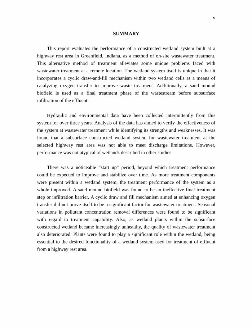
This report evaluates the performance of a constructed wetland system built at a highway rest area in Greenfield, Indiana, as a method of on-site wastewater treatment. This alternative method of treatment alleviates some unique problems faced with wastewater treatment at a remote location. The wetland system itself is unique in that it incorporates a cyclic draw-and-fill mechanism within two wetland cells as a means of catalyzing oxygen transfer to improve waste treatment. Additionally, a sand mound biofield is used as a final treatment phase of the wastestream before subsurface infiltration of the effluent. Hydraulic and environmental data have been collected intermittently from this system for over three years. Analysis of the data has aimed to verify the effectiveness of the system at wastewater treatment while identifying its strengths and weaknesses. It was found that a subsurface constructed wetland system for wastewater treatment at the selected highway rest area was not able to meet discharge limitations. However, performance was not atypical of wetlands described in other studies.
There was a noticeable “start up” period, beyond which treatment performance could be expected to improve and stabilize over time. As more treatment components were present within a wetland system, the treatment performance of the system as a whole improved. A sand mound biofield was found to be an ineffective final treatment step or infiltration barrier. A cyclic draw and fill mechanism aimed at enhancing oxygen transfer did not prove itself to be a significant factor for wastewater treatment. Seasonal variations in pollutant concentration removal differences were found to be significant with regard to treatment capability. Also, as wetland plants within the subsurface constructed wetland became increasingly unhealthy, the quality of wastewater treatment also deteriorated. Plants were found to play a significant role within the wetland, being essential to the desired functionality of a wetland system used for treatment of effluent from a highway rest area.

1
CHAPTER 1
INTRODUCTION 1.1 PROJECT BACKGROUND Until the mid twentieth century, wastewater generated from industries and consolidated areas were dumped into nearby lakes, rivers, and other water bodies. As a result, these water bodies became highly polluted and posed a serious threat to public health and safety. These incidents raised public awareness about water quality issues. To address these concerns, the Federal Water Pollution Control Act (FWCWA) was enacted in 1946, and is the first legislative effort to deal with water quality problems. The act was amended numerous times until it was recognized and expanded in 1972, and formed the basis for the current Clean Water Act (CWA). This act made it unlawful for any person or entity to discharge any pollutants from a point source into navigational waters without a permit. Conventional treatment plants are known to expend a lot of energy. In the United States, for small communities (less than 10,000 population), construction costs vary on an average between $10 and $15 billion nationwide (Hammer, 1997). Moreover, complete sewage treatment for all the residents in the United States is unlikely, and in some cases undesirable because of geographic, economic and sustainability reasons (Crites and Tchobanoglous, 1998). In the United States alone, more than 60 million people live in homes that are served by decentralized collection and treatment systems. Moreover, because of reduction in funding for large sewage treatment systems, many small communities in the United States have turned to onsite sewage treatment technologies. One of the technologies is the use of wetlands for wastewater treatment. In recent times, wetlands have gained popularity over conventional treatment options for small communities, and for businesses located at decentralized locations. Even though natural wetlands have received wastewater from many sources, but they have been recognized as a cost effective treatment system only relatively recently. The goal of constructed wetlands (CWs) is to use the treatment mechanisms of natural wetlands to reduce downstream pollutant discharges. In wetlands, the physical, chemical,
2
and biological processes required for treatment occur in a natural environment instead of synthetic reactor tanks, or basins with artificial chemicals, as in conventional treatment plants. Wetland systems are touted as being low-maintenance technologies, as opposed to conventional treatment plants that require skilled personnel to be present on site. As a result, natural wetlands are often preferred for treatment of wastewaters. Because of the effectiveness of wetlands at low cost, many developing and developed countries over the last 10 to 15 years have chosen to use them for wastewater treatment for small communities. A wetland system in Tanzania has improved the influent wastewater quality by reducing nitrogen concentration by 70%, chemical oxygen demand by 90%, and almost 100% reduction of total coliform (Mbuligwe, 2005). The final effluent is being used for irrigation. In India, a wetland system that was constructed for a school has successfully reduced the ammonia (66-73%), phosphorus (23-48%), and biological oxygen demand (78-91%) (Juwarkar et al., 1995). A number of studies in United States have also shown significant removal efficiency by wetland systems (Steer et al., 2005; Huang et al., 2000). Wetlands have been found suitable for tropical climates (Kantawanichkul et al., 1999), and many European countries have found that wetlands can perform reasonably even in cold climates (Maehlum and Stalnacke, 1999; Maehlum et al., 1995; Haberl et al., 1995). These systems use either single or multiple wetland cells for treatment. In multiple-cell systems, each cell might have different treatment objectives, but their combined effect can improve performance over a single-cell system. Success of wetlands in these and other past studies have prompted the Indiana Department of Transportation (INDOT) to investigate the use of wetlands for the treatment of wastewater generated from highway rest areas. 1.2 PROBLEM STATEMENT Wastewater treatment may be difficult and costly at highway rest area facilities in Indiana, and thus is a topic of interest to both the Indiana Department of Transportation (INDOT) and Purdue University. The Greenfield rest area faces many common problems encountered at rest area facilities along highways, along with some unique ones (Chan et al., 2004). First, rest areas are

3
typically found in such remote locations that sewage systems may not be available or are far away. In the case of the Greenfield rest area, a sewer line greater than three miles in length was installed to carry wastewater back to the municipal wastewater treatment plant of the city of Greenfield. Second, the wastewater produced at rest areas is high-strength and has very concentrated levels of BOD and nitrogen. The strength of the wastewater is further increased by use of low flush toilets and flow-restrictive faucets that were installed to conserve water in the rest stop. Specific to the Greenfield rest area is the long sewer line through which the waste must travel three to four days on average. This prolonged retention time in absence of oxygen causes further breakdown of nitrates into ammonia, increasing contaminant concentration, which also creates an odor problem at the city’s lift station. There is a possibility that the city of Greenfield may impose surcharges in addition to the sewage bill as a result of the increased concentration of BOD and ammonia. Third, wastewater flow varies and is particularly affected by peak flows during traffic hours or holidays. Unstable flow rates make the implementation of any treatment system difficult due to the stress and instability encountered. Last, limited budgets result in a lack of manpower to monitor and maintain the system for optimum performance. Because of these limitations (remote location, high wastewater strength, high variability in wastewater flow, and limited personnel), on-site treatment of effluent is a practical solution to help eliminate costly surcharges for wastewater treatment. Many methods of on-site treatment are currently in practice including dosing fields, aeration ditches, lagoons, ponds, and septic systems. The highway rest area in Greenfield has a working subsurface constructed wetland system. Natural systems such as constructed wetlands have disadvantages and advantages over conventional technologies such as a wastewater treatment facility (Table 1.1). In order to address the problems previously discussed, a subsurface constructed wetland system for wastewater treatment and disposal was proposed by RQAW and J. F. New and Associates. The selected project location was a rest area serving users of Interstate 70 passing through Greenfield, Indiana (about 30 miles east of Indianapolis). The facility was built in 2003 at the rest area site (see Figure 1.1 for location, and Figure 1.2 for schematic) to provide pretreatment on site before discharging the wastewater to the municipal sewer. The wetland system was made operational from early 2004. This specific system was built to see if wetlands could serve as onsite treatment facilities for rest areas.

4
Table 1.1 Conventional water treatment technologies versus constructed wetland systems Conventional Technologies Constructed Wetland Systems Advantages:
1. Small foot print. 2. Proven technologies. 3. Ability to treat large volume and flow rate
of wastewater. 4. Is already in place.
Advantages: 1. Minimal energy requirement. 2. Common pollutants transformed to
harmless byproducts. 3. Potentially small operating and
maintenance costs. 4. Positive public perception. 5. Potential as an ecological habitat.
Disadvantages: 1. Depletion of nonrenewable resources and
the environmental consequences of burning of fossil fuel.
2. Possible generation of undesirable byproducts.
Disadvantages: 1. Large foot print. 2. Relatively large capital costs. 3. Lacking thorough scientific understanding
of the technologies and natural processes.
Figure 1.1 - Location of the Greenfield rest area
Figure 1.2 - Schematic of the constructed wetland wastewater treatment system at the rest area in
Greenfield, IN

5
The rest area was designed to treat an average flow rate of 5,000 gallons per day. The treatment system can receive wastewater generated from two separate buildings situated at opposite sides of the east and westbound lanes, respectively. 1.3 RESEARCH OBJECTIVES The ultimate goal of the ongoing research is to determine the practicality of the implementation of constructed wetland systems as a means of wastewater treatment and disposal at highway rest areas in Indiana. In order for such a system to be successful it must meet regulatory limits for surface and subsurface discharges of key pollutants based on concentration. Surface discharge concentrations may be found in Table 1.2. This report supplements the breadth of knowledge of this topic by examining a variety of tangible issues and presenting the findings along with recommendations. Table 1.2 - Surface water discharge limitations (Source: Indiana Administrative Code; 327 IAC 5-10-4)
Average Concentrations (mg/L) Pollutant Monthly Weekly CBOD5 10 15 Total Suspended Solids (TSS) 12 18 T. Ammonia, as N Summer (May through November) 1.1 1.6 Winter (December through April) 1.6 2.4
The research goals were: 1. To evaluate a fill-and-drain subsurface constructed wetland system for wastewater
treatment based on effluent discharge concentrations of key contaminants, BOD5, TSS, NH3-N, the dependant variables.
2. To overlay hydraulic and environmental data sets to determine treatment effectiveness of this wetland system based on concentration removal, seasonal variations, mass flux reduction, and flow reduction.
3. To analyze the practicability of a sand mound biofield as a means of waste treatment and disposal through infiltration.
4. To determine the effect of wetland plant media presence on the treatment capability of a subsurface constructed wetland.

6
This analysis is supplemented with a qualitative investigation of wetland plants, correlating treatment effectiveness with plant health, selection, and orientation. Recommendations regarding optimal schemes to maximize treatment capabilities are also explored. Through appraising the effectiveness of this subsurface constructed wetland and through investigating these topics of interest, it is the goal of this report to provide further insight into this technology, particularly in its implementation at rest areas in Indiana. This is perhaps the first wetland system in United States that has a network of cells and treats wastewater from a highway rest area. INDOT wants to treat this wetland system as a test site. It was hoped that if this wetland was successful in meeting the regulations for various effluents, then the wetland will be used as “reference wetland” for other rest areas in the state. Moreover, the experience gained at this site could be used for designing and building similar facilities at other sites. 1.4 ORGANIZATION This report covers a number of facets regarding wastewater treatment at a highway rest area. Chapter 1 provides an introduction to the topic of constructed wetlands and identifies the scope and objectives of the research. Chapter 2 denotes the various experimental methods used to collect data. Chapter 3 discusses the importance of wetland plants. A literature review is included in this chapter. Chapter 4 discusses wetland treatment performance, where hydraulic and environmental data are analyzed and presented. An analysis of wetland plant performance is also included. Chapter 5 summarizes the conclusions reached through the data analysis and discusses lessons learned. Appendix A contains a case study that supplements the research presented herein, with particular relevance to wetland plants. Appendix B presents a complete project timeline highlighting important dates, project meeting notes, and significant wetland activity.

7
CHAPTER 2
EXPERIMENTAL METHODS
2.1 KEY ANALYSIS OBJECTIVES The environmental treatment capabilities of the wetland system were measured in terms of Biochemical Oxygen Demand (BOD5), Total Suspended Solids (TSS), and Ammonia-Nitrogen (NH3-N) concentrations. These parameters of the wastewater were tested because they have been accepted as standard methods, have been used in many previous studies, and are used by governing bodies as measures of the quality of treated waste streams. 2.2 DATA COLLECTION Field samples were collected in disinfected 1000 ml plastic bottles provided by ISCO. Samples were obtained on a monthly basis from each automated sampler (AS-1 through AS-4, see Fig 1.2 for locations) as well as form the biofield and surge tank. Samples were sealed in individual bottles and kept in a sealed bucket until analysis at the Purdue University Laboratory for waste characteristics. If laboratory analysis had to be postponed, samples were refrigerated to maintain acceptable temperature, and were isolated from laboratory contaminants. Samples were normally analyzed within 6 hours of collection. In a worst case scenario, some samples were analyzed within 48 hours of collection. The analysis protocol was adopted earlier by Dr. James E. Alleman and N. Shah, and was continued by T. Konopka. 2.3 STANDARD ANALYSIS PROCEDURES Quantities and concentrations of contaminants present in the wastewater samples collected at the rest area were analyzed according to the standard procedures and

8
calculations presented in the Standard Methods for the Examination of Water and Wastewater (17th ed.). BOD5 concentrations were determined according to procedure 5210 B. 5-Day BOD Test. Seed used for oxidizing biodegradable organic matter in samples was obtained from the West Lafayette Wastewater Treatment Plant. Nitrogen concentrations were determined according to procedure 4500-NH3 F. Ammonia-Selective Electrode Method. This method measures nitrogen in the form of ammonia, where dissolved ammonia (aqueous NH3 and NH4
+) is converted to aqueous NH3 by raising pH of the sample to above 11 with a strong base. Total suspended solids were determined according to procedure 2540 D. Total Suspended Solids Dried at 103-105ºC. 2.4 QUALITY ASSURANCE AND QUALITY CONTROL Quality Assurance measures were implemented during the procedures used throughout sampling and analysis in order to produce accurate and precise results. These measures helped in preventing bias, minimizing random error, and eliminating systematic error. Quality Control measures were taken to help produce accurate and precise results through the daily functions carried out during the collection and analysis of samples. Proper cleaning of sampling equipment and bottles, calibration of testing instruments, and analysis of blanks, replicates, and spikes helped ensure the quality of laboratory procedures. The Purdue University environmental laboratory manager, Changhe Xiao, provided laboratory training, and he was also available to help ensure laboratory quality control standards. All chemicals and reagents used in the laboratory were analytical grade or better, and stored away from direct sunlight. Stock chemicals and reagents were always transferred to a clean container prior to weighing. After each use, glassware, plastic ware, or other laboratory equipment was washed with detergent, thoroughly rinsed with water, and finally rinsed with DI water. After drying, all equipment was stored in a dry cabinet. The laboratory where samples were analyzed was kept clean and organized. The room temperature was kept as constant as possible, and air quality was maintained as best as possible. Standard operating procedures reflecting university laboratory regulations were followed for all laboratory procedures.

9
2.4.1 BIOCHEMICAL OXYGEN DEMAND Dissolved oxygen (DO) was measured using an YSI DO-meter, model 55. Calibration and maintenance of the DO Meter was performed according to the manufacturer’s specified procedures. The probe membrane was replaced as necessary, usually after the analysis of 3 lots of wastewater samples. Aeration of dilution (DI) water in a plastic container was accomplished through supplying organic-free filtered shop air to the container. DI water was stored in light shielded containers, sealed with a loose container lid to allow a free exchange of air without contamination. Nutrients for the DI water were prepared in the laboratory and equilibrated to 20.5ºC when in use and sealed when not in use. Seeded DI water blanks were used as a check on the quality of seeded DI water. The DO uptake of seeded DI water in 5 days was checked to be between 0.6-1.0 mg/L. The quality of the unseeded DI water was checked by making BOD5 measurements on a standard solution of 150 mg glucose/l and 150 mg glutamic acid/l. The 5-day BOD measurement of a 2% dilution of the glucose-glutamic acid standard solution was checked to be around 198 mg/L. All samples were well mixed before transferring to BOD bottles and were equilibrated to the appropriate temperature if they were cooled before use. It was ensured that no air bubbles were present in the BOD bottles before incubation. Round glass stoppers were used along with water seals on bottles to guarantee an adequate seal and to prevent drying. All BOD bottles were appropriately labeled. All BOD bottles containing desired dilutions, seeded dilution water blanks, and glucose-glutamic acid checks were incubated at 20.5ºC for 5 days in a dark storage area. BOD bottles were also rotated to hold different samples after each sample lot analysis. 2.4.2 AMMONIA ION SELECTIVE ELECTRODE METHOD The selective electrode method works on the principal of diffusion of gases across a permeable membrane. The electrode detects ammonia and the electrode potential (mV) as it diffuses through a hydrophobic gas-permeable membrane and reaches partial pressure equilibrium on both sides of the membrane. The amount of ammonia that passes through the membrane is proportional to the concentration of ammonia in solution.

10
For the ammonia selective electrode laboratory procedure, an Orion Ammonia Electrode model 95-12 was utilized. Calibration and maintenance of the electrode was performed according to the manufacturer’s specified procedures. When not in use, the electrode was stored according to manufacturer’s guidelines. The probe membrane was replaced as necessary, usually after the analysis of 3 lots of wastewater samples. Interferences (caused by volatile amines) in electrode readings were occasionally observed. Interferences may increase the charge on the electrode membrane, which may cause a high measurement. If readings during the preparation of the standard curve were not within an expected range (i.e. readings were extremely high), or if the slope of the standard curve did not appear normal, it was assumed that interferences had affected the membrane, which required the replacement of the membrane. Samples were warmed to room temperature before analysis if they were refrigerated. The temperature of standards and samples remained consistent during calibration and testing. Samples and standards were stirred slowly with an insulated magnetic stirrer so that air bubbles were not sucked into solution and allowed to form on the membrane. 1 mL of 10 N NaOH was added to all standards and samples to increase pH to 11; this was done only after the electrode was immersed in the solution to prevent the loss of ammonia gas. The electrode was allowed to stabilize before recording mV values. The electrode was rinsed between each standard and sample with ammonia-free water. Ammonia-free water was prepared by adding 1 mL concentrated sulfuric acid or chlorine to distilled water, which was then protected from atmospheric contamination. Stock ammonium chloride solution was purchased commercially, while standard ammonium chloride solution was prepared in the laboratory. A calibration curve on a logarithmic scale was generated by measuring the electrode potential for different concentrations of a standard solution of NH4Cl (1, 10, 100 and 1000 ppm as N). While taking the readings, a pH adjusting solution of methanol and sodium hydroxide was added to maintain high pH during the reaction. Using the calibration curve, unknown concentrations of ammonia in the samples were determined. Analysis of spiked samples was used to determine the accuracy, or bias, of the analysis. The amount of spike was usually twice the concentration of the sample being analyzed. To generate the calibration curve, the linear regression function on a computer spreadsheet was utilized. The use of this standardized statistical procedure produced consistent equations for the “best-fit” line, eliminating the guesswork or bias with a

11
hand-drawn line. Calibration curves were checked for accuracy by using the calibration equation to convert the instrument response for the calibration standards into respective concentrations based on the established calibration curve. Reasonable agreement between the “true”, laboratory-prepared concentrations and the calculated concentrations from the calibration curve were ensured. Calculated concentrations were within 5 - 10% of the “true” concentrations. 2.4.3 TOTAL SUSPENDED SOLIDS In order to get accurate results, 3 replicates of each sample (from each sampling point) were analyzed. Whatman filter papers, number 934-AH, were used for the procedure. In determining total suspended solids, samples were dried at 105ºC. Filters are dried in an oven at 105ºC for at least 1 hour. After drying, filters were stored in a cool and dry area until use. In measuring weights, the balance used was always zeroed before weighing filters. Samples were well mixed and unrepresentative particles were avoided when measuring volumes. Samples were filtered under vacuum, after which filters were washed with 3 successive portions of distilled water. Filters with samples were then dried, and cooled before weighing. Some samples were dried overnight on occasion to check drying efficiency.
12
CHAPTER 3
WETLAND PLANTS
3.1 IMPORTANCE OF WETLAND PLANT MEDIA Constructed wetlands, similar to naturally occurring wetlands, are outfitted with one or more types of wetland plants, in combination with a rock or soil media in which they grow. The plant media within a wetland cell provides a variety of important functions that contribute to the well-being of the system and to wastewater treatment capabilities. Wetland plants sprout roots within the wetland which serve two main functions. Roots provide a surface for beneficial bacteria to grow on, allowing for the consumption and transformation of pollutants present in the influent waste stream. Roots also foster greater oxygen transfer from the atmosphere throughout the wetland. Oxygen within the system promotes adequate nitrification, which directly affects the treatment of ammonia. Plants within a wetland also consume water, thus removing it through transpiration. In a constructed wetland system, water transpiration through plants along with evaporation decreases effluent production. Evapotranspiration rates will vary depending on plant species and density, but rates from 1.5 to 2 times the pan evaporation rate have been reported in the literature (US EPA, 2000). Wetland plants also play a role in winter performance of constructed wetlands by reducing the heat-loss effects of wind and by insulating the wetland from cold temperatures. Aside from their chemical, physical, and biological benefits, wetland plants have the intrinsic value of being aesthetically pleasing. Typical wetland plants found in constructed wetland systems include Carex lacustris, Scirpus acutus, Typha latifolia. 3.2 LITERATURE REVIEW A study performed relating effect of ammonia concentration to biomass production of five common wetland plants in a subsurface wetland application concludes that species with greater biomass could remove more nutrient ammonia from influent wastewaters than those with less biomass (Hill et al., 1997). Monocultures of Juncus roemerianis,

13
Sagittaria latifolia, Phragmites australis, Scirpus acutus, and Typha latifolia were studied under average concentrations of influent NH3-N ranging from 20.5 mg/L to 82.4 mg/L. Significant differences in dry matter production were noticed. Under the testing conditions, dry matter production of Juncus reomerianis is at an extreme variance with no explanation, and the species shows extreme stress as little or no growth occurred. Of the remaining species, Phragmites australis has the greatest dry weight (17.4 g/m2) and is not affected by ammonia concentrations. Typha latifolia and Scirpus acutus produce relatively similar dry weights of 11.5 and 10.5 g/m2 respectively. Scirpus acutus dry matter production is maximized in the 30-50 mg/L of NH3-N. Sagittaria latifolia is not affected by NH3 concentrations but produces the least amount of dry matter with 8.8 g/m2. The conclusion of the study is that harvesting a species with greater biomass could remove more nutrients on a per area and time basis (Hill et al., 1997). Another study found seasonal variation in COD removal in Carex rostrata, Scirpus acutus, Typha latifolia and an unvegetated control (Stein and Hook, 2005). Cold and warm seasons were simulated with temperatures of 4ºC and 24ºC, respectively. Results of the study show Carex rostrata to have improved removal of COD at 4ºC versus 24ºC. Scirpus acutus also shows improved removal of COD at colder temperatures versus warmer, but removal is slightly worse with the Carex rostrata monoculture. Sulfate reduction is limited by organic carbon availability at 24ºC, but is especially strongly reduced in cold temperatures. Typha latifolia shows decreased removal of COD at 4ºC versus 24ºC. Sulfate reduction is also limited by organic carbon availability at 24ºC, and reduction is even lower at cold temperatures. Typha latifolia has poor redox potential year-round. An unvegetated microcosm has the poorest removal of COD and sulfates and has the poorest redox potential. At 4ºC, COD removal is best with Carex rostrata, followed by Scirpus acutus, Typha latifolia, and the unplanted control (Stein and Hook, 2005). Anaerobic microbial metabolism is generally favored during active plant growth at warm temperatures, when most oxygen is believed to be consumed within the root. Aerobic microbial respiration is at times favored during dormancy at cold temperatures, when root respiration is lower and more oxygen is available to microbes in the root zone (Stein and Hook, 2005). Scirpus acutus and Carex rostrata are most capable of increasing root-zone oxygenation during periods of plant dormancy at low temperatures, and this increase is believe to be sufficient enough to modify the overall chemistry of a wetland (Stein and Hook, 2005).
14
Different plant species’ capacities to oxidize the root zone causes them to respond differently to seasonal cycles of growth and dormancy. Species’ effects on wastewater treatment are most pronounced in winter. Physiological response of some plant species to seasonal dormancy and lower temperature (4ºC) permits increased oxygen transfer to the root zone of subsurface flow wetlands. The potential for plants to enhance aerobic treatment processes is more limited during periods of active plant growth and higher temperatures (24ºC). Warmer temperatures enhance removal at low COD concentrations but reduce removal at high concentrations (Stein and Hook, 2005). Generally, temperature is a poor predictor of seasonal performance. However, effects of plants on seasonal performance patterns can be explained by seasonal variation in root-zone oxidation. The effects of plants on performance are frequently greatest during the coldest periods (dormancy) (Stein and Hook, 2005). Plant species selection may be more important to cold-season than to warm-season performance. Planted constructed wetland systems as compared to unplanted systems show enhanced nitrogen and phosphorus removal, but only small improvements in disinfection, BOD, COD and TSS removal (Tanner, 2001). Research was carried out under hydraulic loading rates of 25-182 mm/day of domestic and agricultural wastewaters with varying levels of preceding treatment, and 8 different plant species. Sizes of pilot scale systems varied from 18-400 m2 and experimental microcosm studies from 0.08-6 m2. In the studies, BOD or COD removal capabilities were nearly unchanged in planted or unplanted systems. However, for paired systems, BOD concentrations are reduced by 2-5 g/m3 for planted beds. TSS removal was also very similar for planted and unplanted systems. Planted wetlands showed a clear trend of improved total nitrogen removal. Enhanced phosphorus and metal mass removal was also observed as compared to unplanted systems. Planted beds showed small but consistent improvements in inactivation rates of fecal coliform and a range of other bacterial indicators as well as lower effluent concentrations of viruses than unplanted systems (Tanner, 2001). Comparison with unplanted controls after ~2 years of operation showed 1.6-6 times greater organic matter accumulation in the presence of plants. Accumulated organic matter provides additional sorption sites, sources of complexing and biochemically active substances, and substrates for microbial processes. This intensifies nutrient cycling, elevating the residence time of nutrients relative to that of wastewaters passing through them (Tanner, 2001).
15
Nitrogen and phosphorus removal capabilities of Scirpus validus, Carex lacustris, Phalaris arundinacea, and Typha latifolia, a mixture of the four, and an unvegetated control were greatly varied (Fraser et al., 2004). These plants are fast-growing, tall stature, “clonal-dominants”, that establish quickly and process a lot of energy (Fraser et al., 2004). Testing was done during the second growing season, since research has shown that in constructed systems, more than one year me be needed to reach “natural wetland conditions” (Sistani et al., 1996). Concentrations of applied nitrogen and phosphorus, high/low levels at 112/26.5 mg/L and 62/15.5 mg/L, respectively, were applied. Under these conditions, Scirpus validus was most effective in nitrogen and phosphorus reduction and high levels of nutrient input. Carex lacustris showed high effectiveness in removal capabilities at high inputs of nitrogen and phosphorus (similar to Scirpus validus), but also had the greatest dry biomass production at both high and low nutrient levels. Phalaris arundinacae was the least effective in nitrogen and phosphorus reduction, with treatment capabilities similar to unvegetated microcosms. Typha latifolia was the slowest to establish of the plants used in the study, and at high nutrient levels, growth was stunted or the plants were killed. Performance of the 4-species mixture was comparable to the removal capabilities of the Typha latifolia monoculture. For this species, removal capability at low nutrient levels was good, but removal capability at high nutrient level was average at best. Unplanted controls consistently had significantly higher nitrogen values than any vegetated microcosms (Fraser et al., 2004). Overall, Carex lacustris and Scirpus validus monocultures showed the best (and similar) performance. Typha latifolia and the 4-species mix, showed similar results, have significantly worse removal capabilities at high nutrient input than Carex lacustris and Scirpus validus monocultures. Unvegetated microcosms and Phalaris arundinacae monocultures had similar performance results; removal capabilities of both were the worst of this study (Fraser et al., 2004). Vegetated microcosms are shown to be more effective at reducing concentrations of total nitrogen and phosphorus from soil lechate than unvegetated microcosms. There is a differential species effect on the potential to reduce nitrogen and phosphorus. Plant mixtures are not necessarily more effective than monocultures at reducing nitrogen and phosphorus (Fraser et al., 2004). Riley et al. (2005) tested ammonium and COD removal capabilities of Typha latifolia, Carex rostrata, and an unvegetated control under constant influent levels of NH4-N (40
16
mg/L) as the nitrogen source and COD (225 mg/L) as the organic carbon source. The year-long study included seasonal changes created by adjusting the temperature of the environment of the microcosms to 24ºC, 14ºC, and 4ºC in the summer, fall/spring, and winter, respectively. Conclusions of the study showed that Carex rostrata had superior year-round organic carbon removal and increased root-zone oxygenation over Typha latifolia and the unplanted control. Ammonium removal was greater in winter than in the summer in the presence of COD in a Carex rostrata monoculture. Ammonium removal by a Typha latifolia monoculture was not affected by season, but half as much COD was removed in the summer season as was removed in the winter season when compared to Carex rostrata. The unplanted monoculture performed the worst in all categories (Riley et al., 2005). 3.3 RATIONALE It is first important to note that COD (Chemical Oxygen Demand) and BOD (Biological Oxygen Demand) tests are similar in that, either chemically or biologically, both tests oxidize organic carbon in wastewater and measure the relative oxygen-depletion effect of a waste contaminant. Both have been widely adopted as a measure of pollution effect. The BOD test measures the oxygen demand of biodegradable pollutants whereas the COD test measures the oxygen demand of biodegradable pollutants plus the oxygen demand of non-biodegradable pollutants that can be oxidized. To measure oxygen demand, BOD relies on bacteria to oxidize readily available organic matter during an incubation period. COD uses strong chemicals to oxidize organic matter. Thus, the studies performed by Riley et al. (2005), Stein and Hook (2005), and Tanner (2001) are relevant and applicable in that their measurements of COD relate to BOD measurements taken at the Greenfield wetland site. There is a growing body of evidence that some wetland species, including Carex rostrata, can enhance the oxygen available for microbial processes in winter over summer (Riley et al., 2005). Plant-mediated oxygen transfer affects water treatment most in winter and, as such, the choice of plants is potentially more important to subsurface flow wetland performance during the winter than during the growing season (Stein and Hook, 2005). Strong differences between species were apparent during cold temperatures and plant dormancy but are minimal at warmer temperatures when plants were actively growing (Stein and Hook, 2005). The efficiency of aerobic respiration over anaerobic respiration
17
is so great that only a modest shift toward aerobic conditions could obscure or even reverse the effect of temperature on microbial activity. Thus, moderate increases in oxygen availability in winter could offset effects of cold temperatures (Stein and Hook, 2005). Increased rates of BOD removal and ammonia oxidation from wastewaters and elevated dissolved oxygen concentrations have been recorded in the root-zone of wetland plants (Dunbabin et al., 1988). Root oxygen release was credited for improved rates of NH3-N removal by stimulating nitrification (Tanner, 2001). Plants primarily affect treatment performance through ecosystem engineering, enhancing key nutrient transformation processes (e.g. nitrification and denitrification) by root-zone oxygen release and supply of organic matter (Tanner, 2001). For Scirpus species grown in wastewater dilutions, Tanner (2001) found that increasing BOD rather than nutrients was the primary environmental factor influencing the depth of root penetration. Also, reduced winter nitrogen removal was attributed to decreased plant uptake during the dormant season and dramatically decreased microbial metabolism at colder temperatures (Kadlec and Knight, 1996). Results of the studies overlap and coincide with each other with regard to plant species and treatment effectiveness. Typha latifolia was least effective, possibly due to its shallow rooting zone and the inability to create an effective environment for various microbial communities (Gersberg et al., 1986). Also, Coleman et al. (2001) showed that there was no significant difference between Typha latifolia monocultures and mixed systems. Carex lacustris, one of the best performers of one study, was noted to have the greatest amount of biomass of the tested species (Fraser et al., 2004). An increase in biomass, both living and dead, was found to enhance rates of denitrification and have improved removal efficiencies of nitrogen. 3.4 CONCLUSIONS DRAWN FROM LITERATURE Unvegetated controls in all the studies consistently showed the same results; they all had poorest removal capabilities in all aspects of wastewater treatment. Planted systems showed enhanced nitrogen and phosphorus removal and improvements in disinfection, BOD, COD and TSS removal (Tanner, 2001). Thus, plants are shown to be valuable to the treatment processes that occur within a subsurface constructed wetland.

18
Typha latifolia is an attractive species for a constructed wetland application because it has been shown to produce more biomass than Scirpus acutus and Sagittaria latifolia (Hill et al., 1997). However, Scirpus acutus produced only slightly more biomass than Typha latifolia, making it nearly as desirable. Although Typha latifolia was not effected by high NH3 concentrations (Hill et al., 1997) or by temperature (Riley et al., 2005), this species showed decreased removal of COD at cold temperatures as compared to warm temperatures, and poor year-round redox potential (Stein and Hook, 2005). Carex rostrata and Scirpus acutus showed improved removal of COD at cold temperatures as compared to warm temperatures (Hill et al., 1997). Carex rostrata had superior year-round organic carbon removal and increased root-zone oxidation over Typha latifolia as well as greater ammonium nitrogen removal in the winter than in the summer in the presence of COD (Riley et al., 2005). However, Scirpus validus was most effective in nitrogen and phosphorus reduction (Fraser et al., 2004). Carex lacustris had great dry biomass production with very effective removal of nitrogen and phosphorus as well. Typha latifolia, on the other hand, was slowest to establish and high nutrient inputs can stunt and kill those plants. The performance of Typha latifolia monocultures had similar performance to mixture of plants, overall (Fraser et al., 2004). The literature provides a practical set of conclusions. First, plants are important to subsurface flow constructed wetlands because of the following reasons: 1. Wetland plant roots provide a structure for microorganisms to adhere to and perform
processes necessary for transformation of nutrients. 2. Wetland plants allow oxygen transfer through their roots, thus increase levels of
oxygen and promoting the oxidation of toxic substances such as ammonia. 3. Wetland plants uptake influent water and are able to remove it through
evapotranspiration, thus decreasing effluent quantities. 4. Wetland plants reduce the heat-loss effects of wind and by insulating the wetland
from cold temperatures. Conclusions can also be drawn from literature regarding qualities of most desirable wetland plants to be used in a subsurface constructed wetland application: 1. Wetland plants with robust biomass production are favored over those which produce
less biomass. Greater root systems foster a greater metabolizing habitat for bacteria within the root zone.

19
2. Seasonal temperatures affect oxygen presence for microbes in the root zone. The winter season is the limiting season, and wetland plants with least effect in performance during this season are best.
3. Wetland plants that are perennial, establish quickly, and process a lot of energy while out-competing other wetland or invasive species will thrive in a constructed wetland system with increased nutrient levels in influent streams.
Plant species selection for a subsurface constructed wetland is crucial in order to be able to achieve desired effluent results. Literature suggests that the most desirable plant geneses for wastewater treatment through wetland technology are Carex and Scirpus. 3.5 CASE STUDY VS LITERATURE REVIEW Before embarking on the Greenfield project, an existing wetland facility was examined for experience. The France Park case study, presented in Appendix A, supports the conclusions of the literature that has been reviewed. Removal capabilities of ammonia from the wetland cells at France Park were found to be very good for the most part, with capabilities as high as 99.4%. It was observed that the plants with the largest root systems were of the Carex and Scirpus geneses. This information is particularly relevant to the conclusions drawn from the literature stating that, based on water treatment capabilities, the Carex and Scirpus geneses would be the best choices for subsurface wetland application. The water treatment results along with an analysis of the plants from the subsurface constructed wetland system at France Park show the qualitative and quantitative results to support the conclusions that plants of the Carex and Scirpus genus are greatly effective at treating wastewater. Although the concept of specific plant orientation among mixed cultures of wetland plants was not explicitly discussed in any literature, conclusions may be drawn from the case study and supplemented by results from other studies. Orienting the two species of plants in a specific and separate arrangement within the same wetland cell prevents two problems that inhibit productivity. Taller or larger plants pose problems to smaller plants in that if they grow tall, they shade the lower plants, thus causing plant stress. Plants with larger or deeper root systems also affect plants with smaller or shallower root systems in that deeper or larger root systems take away water and nutrients from plants that have

20
shallower and smaller root systems. Additionally, species with shallow root systems have to compete with invasive plant species that essentially begin their growth by drawing water and nutrients from the uppermost level of water and nutrients. Within a constructed wetland cell, these issues are important because competition between plants can ultimately lead to the extinction of certain wetland plants within wetland cells as has been noticed at the Greenfield rest area. Species that are planted and then lost due to these reasons are effectively a waste of money and are detrimental to the nutrient removal efforts of other more effective plants, which also could have been planted in place of the ineffective species.

21
CHAPTER 4
WETLAND SYSTEM PERFORMANCE
4.1 FLOW CHARACTERISTICS Flow data throughout the wetland system has been collected from the time the system was constructed and outfitted with the flow measuring devices. Over the study period, however, flow data collection was not entirely consistent. For example, some periods of flow data collection had intervals as frequently as one minute, while other data were gathered based on five minute intervals or as daily averages. Moreover, there were periods of time that some flow measuring equipment was out of commission. No flow data was available as a result (for example, from January to July of 2006). In addition to flow data being available sporadically and recorded in an inconsistent matter, there are instances where the data is erroneous due to errors in the flow reading capability of the equipment or mechanical errors causing unwanted flow conditions through the wetland system. Sultana et al. (2006) developed a hydraulic model for the entire system where all the logic of operations of lift stations and actuators was explicitly represented. This study provided a critical assessment of the flow data. In order to use the available flow data appropriately with the treatment data, flow conditions were observed during a five day window around the date of wastewater sampling for each sampling point. The flow data for a given date is an average daily flow rate calculated from of the best available data from the day of a sampling date, two days before that day, and two days after. This method of determining the flow rate for a given sampling day helps alleviate the errors of possible erroneous data, and also provides a probable flow rate for a sampling day when the actual flow data was not available. One of the greatest errors in flow data was found in the data collected from flow meter F-3, measuring flow directly out of wetland cell W-3. Errors in data collected from flow meter F-2 were also observed. These errors were due observed flow values being within ranges where instrumental error tends to be the highest. As an alternate method of determining flow out of wetland cell W-3, flow data was estimated for this point in the system through the use of data collected from the weather station and combining it with
22
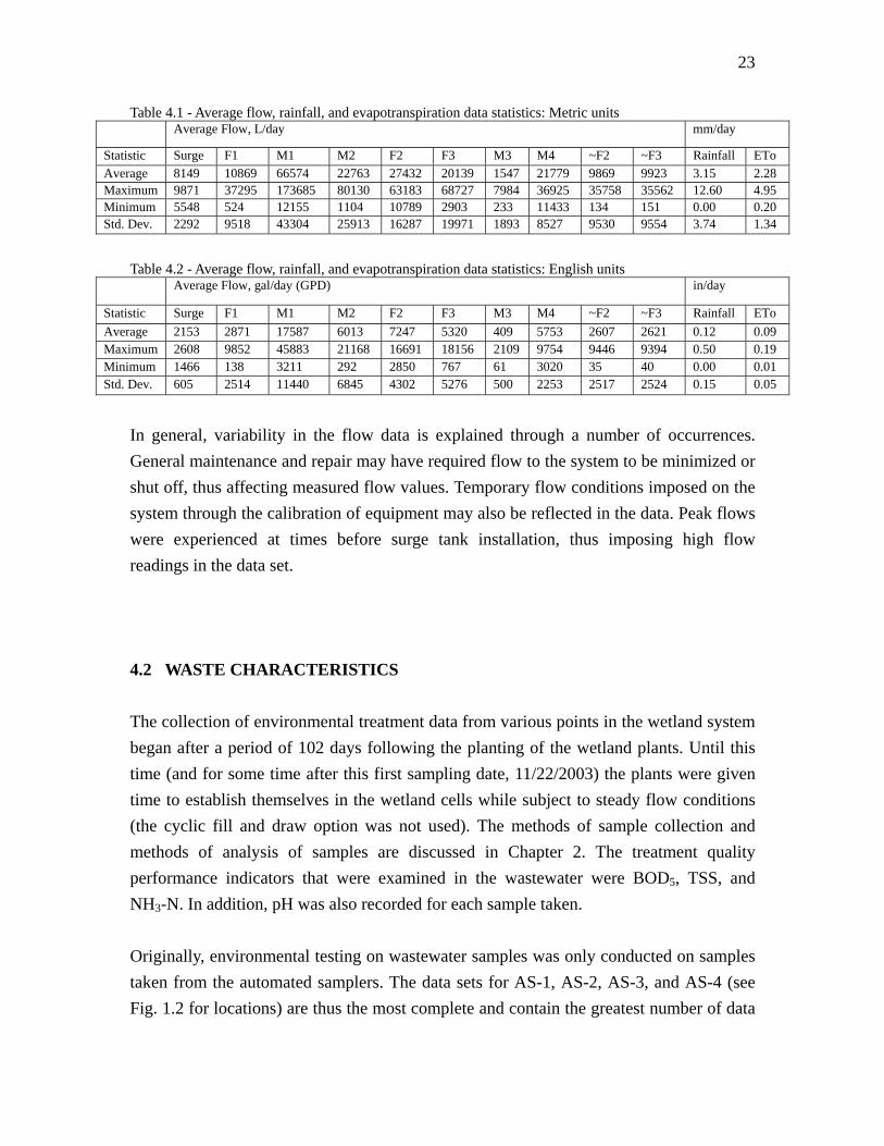
the data from flow meter F-1, found between the septic tanks. Similarly, flow out of the parallel wetland cells W-1 and W-2 at F-2 was also estimated for this point in the system. The weather station was able to provide rainfall and evapotranspiration (ETo) data, which was also averaged in the same manner as the flow data over a five day window. Average evapotranspiration and rainfall values were quantified into average daily flows by multiplying their intensities by the combined area of the wetland cells. Taking the average daily flow value from flow meter F-1 and adding the average flow difference resulting from rainfall and evapotranspiration provided a more reliable estimate of the flow rates at F-3 and F-2. Table 4.1 and 4.2 show a statistical comparison of all average flow data at all possible flow measuring points in the system from all available points correlated with wastewater sampling dates. In some cases, the data varies significantly between the various flow measuring points. For example, the average flow found at the flow meter F-1, between the septic tanks but before recirculation, is 2871 gallons per day (gpd). This value is consistent with surge tank flow readings, but significantly lower than the flow data found at flow meters F-2 or F-3, found directly before and after wetland cell W-3, respectively. The average flow data at F-2 was found to be 7247 gpd and at F-3 was found to be 5320 gpd. This greatly increased flow from the entrance to the system to a point within the system cannot be easily explained. The data from the weather station does not support a claim that infiltration due to rainfall caused such an increase in flow. However, the estimated flow rate ~F3 shows an average daily flow value of 2621 gpd, and the estimated flow rate ~F2 shows an average daily flow value of 2607 gpd, values which are much closer to the 2871 gpd measured at F-1, supporting the estimates as reasonable. A final consideration in the flow data was in the differences observed from the surge flow data as compared to that of F-1. The surge tanks became the ultimate flow entrance point into the wetland system. In theory, the flow recorded at the surge tank should be the same as that recorded at F-1, where there is no possibility for infiltration or water loss between these points. However, the data shows that the average daily flow recorded at the surge tank was 2153 gpd while the average daily flow recorded by F-1 was 2871 gpd (refer to Table 4.2). The standard deviations for these average values vary greatly. The standard deviation for the average daily flow of the surge tank is just 605 gpd, while for F-1 the standard deviation is 2514 gpd. Because of this, there were instances where the surge flow data were used in place of F-1 data in calculations involved in changes in mass flux and cumulative contaminant mass removal ratio (explained in detail later this chapter).
23
Table 4.1 - Average flow, rainfall, and evapotranspiration data statistics: Metric units Average Flow, L/day mm/day
Statistic Surge F1 M1 M2 F2 F3 M3 M4 ~F2 ~F3 Rainfall EToAverage 8149 10869 66574 22763 27432 20139 1547 21779 9869 9923 3.15 2.28 Maximum 9871 37295 173685 80130 63183 68727 7984 36925 35758 35562 12.60 4.95 Minimum 5548 524 12155 1104 10789 2903 233 11433 134 151 0.00 0.20 Std. Dev. 2292 9518 43304 25913 16287 19971 1893 8527 9530 9554 3.74 1.34
Table 4.2 - Average flow, rainfall, and evapotranspiration data statistics: English units
Average Flow, gal/day (GPD) in/day
Statistic Surge F1 M1 M2 F2 F3 M3 M4 ~F2 ~F3 Rainfall EToAverage 2153 2871 17587 6013 7247 5320 409 5753 2607 2621 0.12 0.09 Maximum 2608 9852 45883 21168 16691 18156 2109 9754 9446 9394 0.50 0.19 Minimum 1466 138 3211 292 2850 767 61 3020 35 40 0.00 0.01 Std. Dev. 605 2514 11440 6845 4302 5276 500 2253 2517 2524 0.15 0.05
In general, variability in the flow data is explained through a number of occurrences. General maintenance and repair may have required flow to the system to be minimized or shut off, thus affecting measured flow values. Temporary flow conditions imposed on the system through the calibration of equipment may also be reflected in the data. Peak flows were experienced at times before surge tank installation, thus imposing high flow readings in the data set. 4.2 WASTE CHARACTERISTICS The collection of environmental treatment data from various points in the wetland system began after a period of 102 days following the planting of the wetland plants. Until this time (and for some time after this first sampling date, 11/22/2003) the plants were given time to establish themselves in the wetland cells while subject to steady flow conditions (the cyclic fill and draw option was not used). The methods of sample collection and methods of analysis of samples are discussed in Chapter 2. The treatment quality performance indicators that were examined in the wastewater were BOD5, TSS, and NH3-N. In addition, pH was also recorded for each sample taken. Originally, environmental testing on wastewater samples was only conducted on samples taken from the automated samplers. The data sets for AS-1, AS-2, AS-3, and AS-4 (see Fig. 1.2 for locations) are thus the most complete and contain the greatest number of data
24
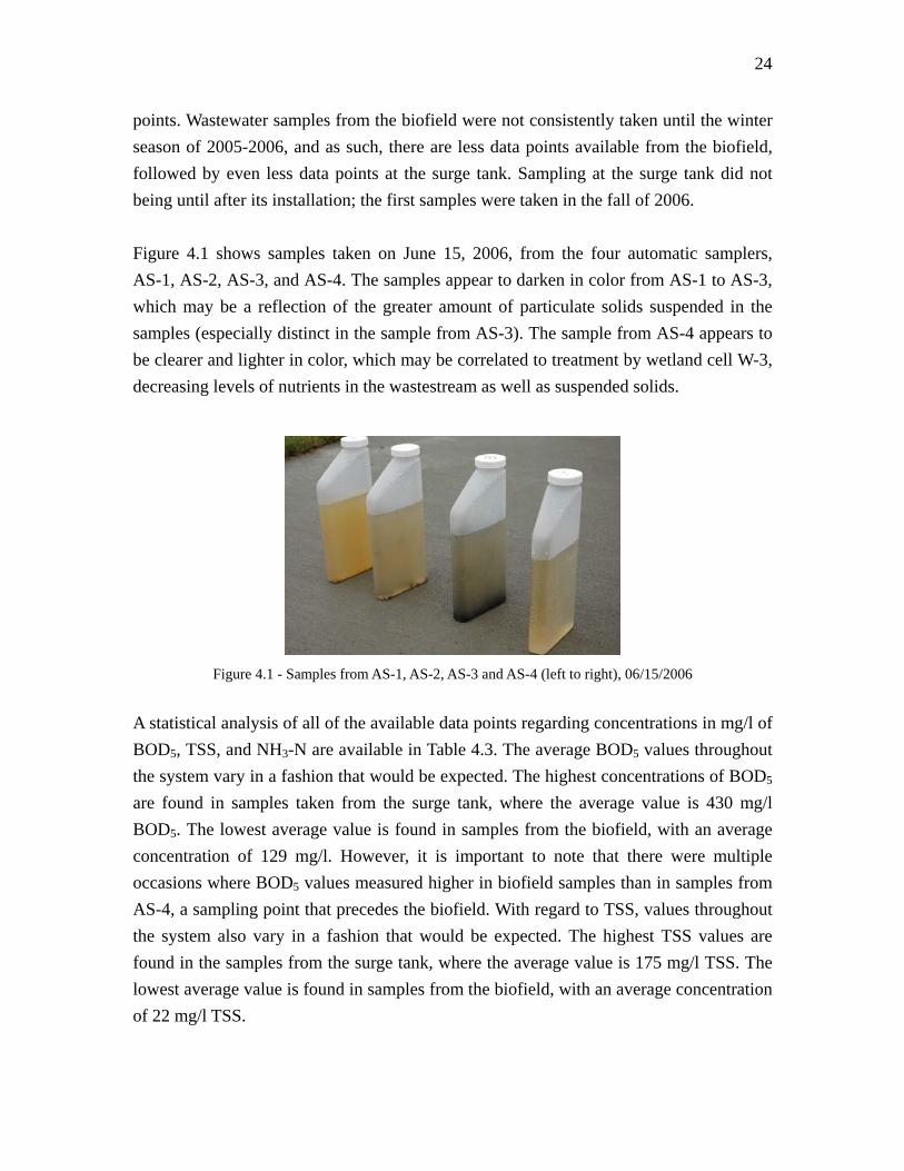
points. Wastewater samples from the biofield were not consistently taken until the winter season of 2005-2006, and as such, there are less data points available from the biofield, followed by even less data points at the surge tank. Sampling at the surge tank did not being until after its installation; the first samples were taken in the fall of 2006. Figure 4.1 shows samples taken on June 15, 2006, from the four automatic samplers, AS-1, AS-2, AS-3, and AS-4. The samples appear to darken in color from AS-1 to AS-3, which may be a reflection of the greater amount of particulate solids suspended in the samples (especially distinct in the sample from AS-3). The sample from AS-4 appears to be clearer and lighter in color, which may be correlated to treatment by wetland cell W-3, decreasing levels of nutrients in the wastestream as well as suspended solids.
Figure 4.1 - Samples from AS-1, AS-2, AS-3 and AS-4 (left to right), 06/15/2006
A statistical analysis of all of the available data points regarding concentrations in mg/l of BOD5, TSS, and NH3-N are available in Table 4.3. The average BOD5 values throughout the system vary in a fashion that would be expected. The highest concentrations of BOD5 are found in samples taken from the surge tank, where the average value is 430 mg/l BOD5. The lowest average value is found in samples from the biofield, with an average concentration of 129 mg/l. However, it is important to note that there were multiple occasions where BOD5 values measured higher in biofield samples than in samples from AS-4, a sampling point that precedes the biofield. With regard to TSS, values throughout the system also vary in a fashion that would be expected. The highest TSS values are found in the samples from the surge tank, where the average value is 175 mg/l TSS. The lowest average value is found in samples from the biofield, with an average concentration of 22 mg/l TSS.

25
Table 4.3 - Average pollutant concentration statistics at sampling points Pollutant Statistic ST AS1 AS2 AS3 AS4 BF
Average 430 337 234 195 147 128 Maximum 444 396 300 259 226 155 Minimum 417 260 122 90 82 105
BOD5 mg/l
Std. Dev. 14 38 61 80 40 66 Average 175 139 87 73 37 22 Maximum 183 220 144 216 60 31 Minimum 165 65 40 32 12 6
TSS mg/l
Std. Dev. 64 26 24 43 14 12 Average 183 194 132 126 106 105 Maximum 204 314 203 184 206 179 Minimum 157 35 30 39 30 0
NH3-N mg/l
Std. Dev. 68 56 48 59 40 62 Average ammonia-nitrogen concentrations show a unique trend among the sampling points. The second sampling point, AS-1, proved to have a greater average concentration of NH3-N than the samples taken from the surge tank, which precedes AS-1. This could be due to the fact that there is a much smaller pool of data points available from the surge tank, and more data needs to be collected in order to have a more accurate average value. The wastewater collected in the septic tanks may have a prolonged residence time in an absence of oxygen that causes ammonia levels to rise. Thus, it is possible that a wastewater sample taken as AS-1 (between the septic tanks) may in fact contain more NH3-N than a sample from the surge tank. It is important to note that the recirculation line connects to the system between the septic tanks ST-1 and ST-2, however, after the automated sampler. The lowest average ammonia-nitrogen concentrations also have significant results. Table 4.3 shows that the average concentration of NH3-N is almost equal at samples taken from AS-4 and the biofield, with concentrations of 106 and 105 mg/l, respectively. It is important to note that the standard deviation of the data from the biofield with regard to NH3-N is also higher than that of the data from AS-4, with values of 62 and 40 mg/l, respectively. This observation in the statistical analysis of the data is contrary to the assumption that NH3-N levels would decrease through the use of the biofield. Regarding pH measurements taken throughout the system, all were generally closely related to each other. An average pH for any given point within the system fell between 7 or 8, with outliers being rather uncommon. Because the pH data was normal as compared to standard pH levels of wetlands and because pH did not change significantly at sampling points throughout the study period, it can be presumed that pH did not have a
26
significant impact on the removal capability of the wetland system. The influence of pH seems to have been minimal and did not change over the course of time. 4.3 ANALYSIS CRITERIA To best utilize the available flow and wastewater treatment data, four significant analysis criteria were determined and applied to six different scenarios to determine the treatment capabilities of the system. Figures presenting data include best fit lines to illustrate trends in data. The slopes of the best fit lines were analyzed for significant differences from zero through standard analysis of variance (ANOVA) calculations. A slope significantly different from zero suggest that, at 95% confidence, the change in the dependant variable is significant over a period of time. 4.3.1 CONCENTRATION REMOVAL This criterion evaluates pollutant concentration removal as a percentage based on differences in concentrations measured between points within the wetland system. Pollutant concentrations have been determined in units of mass of contaminant per volume of wastewater. This analysis criteria shows how these values differ in a given wastewater sample set, thus measuring treatment performance based on concentrations. 4.3.2 MASS FLUX REDUCTION This analysis criterion first combines flow data with contaminant concentration data to determine levels of pollutants as masses per day at various points. By comparing mass flux entering the system and mass flux exiting the system between given points, it is possible to measure treatment performance based on the percentage reduction in mass flux through the system.

27
4.3.3 FLOW REDUCTION This criterion evaluates flow reduction as a percentage based on differences in measured flow values between points within the wetland system. This analysis criteria is an indicator of system performance. 4.3.4 SEASONAL VARIATION This criterion combines the independent variable of time with the concentration removal data in order to show seasonal variation in the removal capability of the key pollutants between locations within the wetland system. This analysis criterion shows whether or not there is a dynamic trend present in pollutant concentration removal. Seasons were determined as shown in Table 4.4. Table 4.4 - Seasons Season Start End Winter December 15 March 14 Spring March 15 June 14 Summer June 15 September 14 Fall September 15 December 14 4.4 CASES EXAMINED 4.4.1 AS-1 - AS-4 This case examines performance of the septic tank along with the three wetland cells. As was mentioned previously, the data set for automated samplers (AS-1 to AS-4, see Fig 1.2) contains the greatest amount of data points. It is important to mention that obtaining enough data points to determine mass flux reductions was difficult based on the fact that a complete set of flow and contaminant concentration data was required for one given date (data point) in order to perform the necessary calculations. Thus, as this case had the most extensive data set, it was possible to perform a reasonable analysis based on all aforementioned criteria. Figure 4.2 and 4.3 show trends in percent contaminant concentration removal capability of BOD5, TSS, and NH3-N between sampling points AS-1 and AS-4 over time. The
28
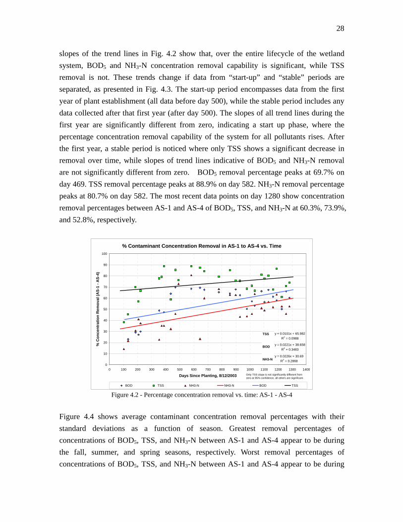
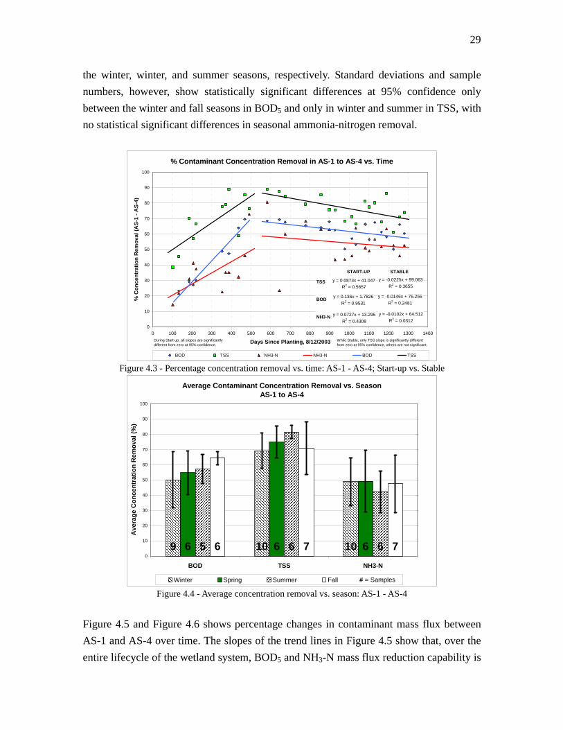
slopes of the trend lines in Fig. 4.2 show that, over the entire lifecycle of the wetland system, BOD5 and NH3-N concentration removal capability is significant, while TSS removal is not. These trends change if data from “start-up” and “stable” periods are separated, as presented in Fig. 4.3. The start-up period encompasses data from the first year of plant establishment (all data before day 500), while the stable period includes any data collected after that first year (after day 500). The slopes of all trend lines during the first year are significantly different from zero, indicating a start up phase, where the percentage concentration removal capability of the system for all pollutants rises. After the first year, a stable period is noticed where only TSS shows a significant decrease in removal over time, while slopes of trend lines indicative of BOD5 and NH3-N removal are not significantly different from zero. BOD5 removal percentage peaks at 69.7% on day 469. TSS removal percentage peaks at 88.9% on day 582. NH3-N removal percentage peaks at 80.7% on day 582. The most recent data points on day 1280 show concentration removal percentages between AS-1 and AS-4 of BOD5, TSS, and NH3-N at 60.3%, 73.9%, and 52.8%, respectively.
% Contaminant Concentration Removal in AS-1 to AS-4 vs. Time
y = 0.0226x + 30.69R2 = 0.2868
y = 0.0221x + 38.658R2 = 0.3483
y = 0.0101x + 65.982R2 = 0.0988
0
10
20
30
40
50
60
70
80
90
100
0 100 200 300 400 500 600 700 800 900 1000 1100 1200 1300 1400
Days Since Planting, 8/12/2003
% C
once
ntra
tion
Rem
oval
(AS-
1 - A
S-4)
BOD TSS NH3-N NH3-N BOD TSS
Only TSS slope is not significantly different from zero at 95% confidence, all others are significant.
TSS
BOD
NH3-N
Figure 4.2 - Percentage concentration removal vs. time: AS-1 - AS-4
Figure 4.4 shows average contaminant concentration removal percentages with their standard deviations as a function of season. Greatest removal percentages of concentrations of BOD5, TSS, and NH3-N between AS-1 and AS-4 appear to be during the fall, summer, and spring seasons, respectively. Worst removal percentages of concentrations of BOD5, TSS, and NH3-N between AS-1 and AS-4 appear to be during
29
the winter, winter, and summer seasons, respectively. Standard deviations and sample numbers, however, show statistically significant differences at 95% confidence only between the winter and fall seasons in BOD5 and only in winter and summer in TSS, with no statistical significant differences in seasonal ammonia-nitrogen removal.
% Contaminant Concentration Removal in AS-1 to AS-4 vs. Time
y = 0.0727x + 13.295R2 = 0.4308
y = 0.136x + 1.7826R2 = 0.9531
y = 0.0873x + 41.047R2 = 0.5657
y = -0.0225x + 99.063R2 = 0.3655
y = -0.0146x + 76.256R2 = 0.2481
y = -0.0102x + 64.512R2 = 0.0312
0
10
20
30
40
50
60
70
80
90
100
0 100 200 300 400 500 600 700 800 900 1000 1100 1200 1300 1400
Days Since Planting, 8/12/2003
% C
once
ntra
tion
Rem
oval
(AS-
1 - A
S-4)
BOD TSS NH3-N NH3-N BOD TSS
TSS
BOD
NH3-N
START-UP STABLE
While Stable, only TSS slope is significantly different from zero at 95% confidence, others are not significant.
During Start-up, all slopes are significantly different from zero at 95% confidence.
Figure 4.3 - Percentage concentration removal vs. time: AS-1 - AS-4; Start-up vs. Stable
Average Contaminant Concentration Removal vs. SeasonAS-1 to AS-4
9 10 106 6 65 6 66 7 70
10
20
30
40
50
60
70
80
90
100
BOD TSS NH3-N
Ave
rage
Con
cent
ratio
n R
emov
al (%
)
0
10000
20000
30000
40000
50000
60000
70000
80000
90000
100000
Winter Spring Summer Fall Series5# = Samples Figure 4.4 - Average concentration removal vs. season: AS-1 - AS-4
Figure 4.5 and Figure 4.6 shows percentage changes in contaminant mass flux between AS-1 and AS-4 over time. The slopes of the trend lines in Figure 4.5 show that, over the entire lifecycle of the wetland system, BOD5 and NH3-N mass flux reduction capability is
30
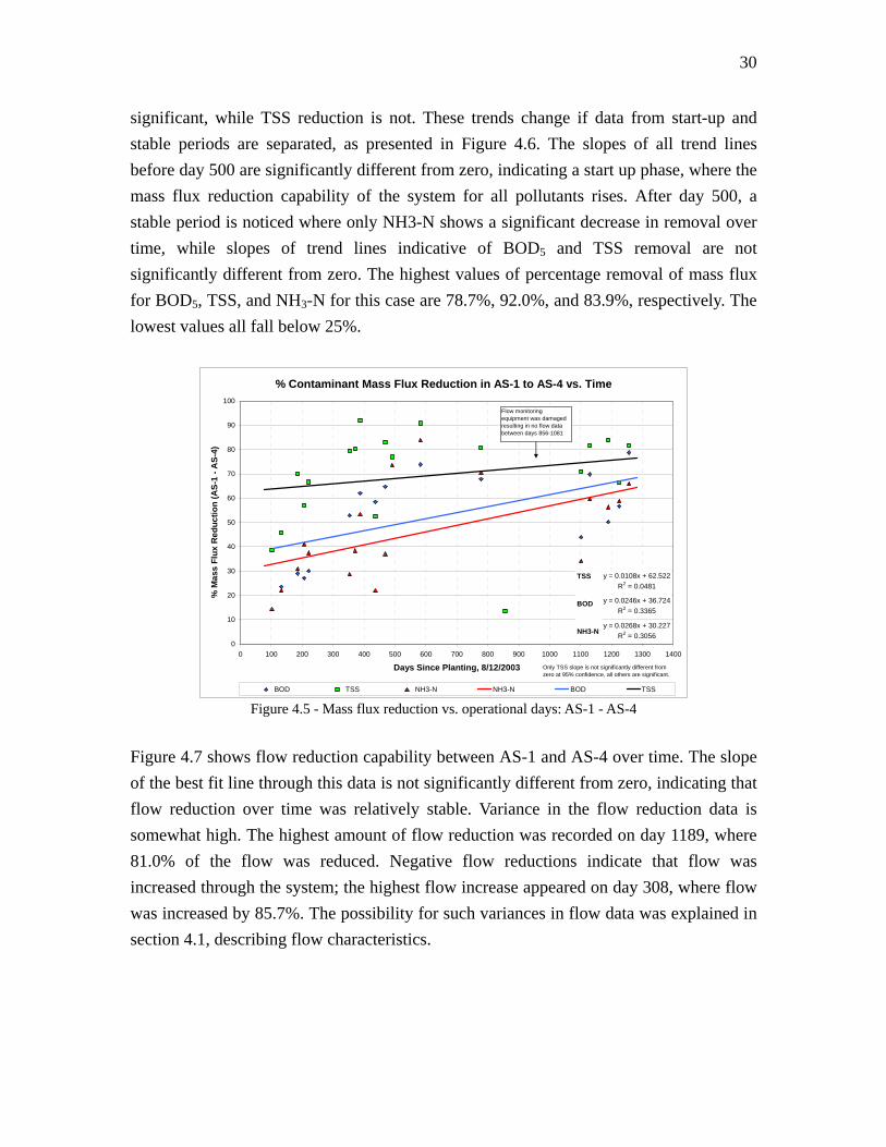
significant, while TSS reduction is not. These trends change if data from start-up and stable periods are separated, as presented in Figure 4.6. The slopes of all trend lines before day 500 are significantly different from zero, indicating a start up phase, where the mass flux reduction capability of the system for all pollutants rises. After day 500, a stable period is noticed where only NH3-N shows a significant decrease in removal over time, while slopes of trend lines indicative of BOD5 and TSS removal are not significantly different from zero. The highest values of percentage removal of mass flux for BOD5, TSS, and NH3-N for this case are 78.7%, 92.0%, and 83.9%, respectively. The lowest values all fall below 25%.
% Contaminant Mass Flux Reduction in AS-1 to AS-4 vs. Time
y = 0.0268x + 30.227R2 = 0.3056
y = 0.0246x + 36.724R2 = 0.3365
y = 0.0108x + 62.522R2 = 0.0481
0
10
20
30
40
50
60
70
80
90
100
0 100 200 300 400 500 600 700 800 900 1000 1100 1200 1300 1400
Days Since Planting, 8/12/2003
% M
ass
Flux
Red
uctio
n (A
S-1
- AS-
4)
BOD TSS NH3-N NH3-N BOD TSS
TSS
BOD
NH3-N
Only TSS slope is not significantly different from zero at 95% confidence, all others are significant.
Flow monitoring equipment was damaged resulting in no flow data between days 856-1081
Figure 4.5 - Mass flux reduction vs. operational days: AS-1 - AS-4
Figure 4.7 shows flow reduction capability between AS-1 and AS-4 over time. The slope of the best fit line through this data is not significantly different from zero, indicating that flow reduction over time was relatively stable. Variance in the flow reduction data is somewhat high. The highest amount of flow reduction was recorded on day 1189, where 81.0% of the flow was reduced. Negative flow reductions indicate that flow was increased through the system; the highest flow increase appeared on day 308, where flow was increased by 85.7%. The possibility for such variances in flow data was explained in section 4.1, describing flow characteristics.
31
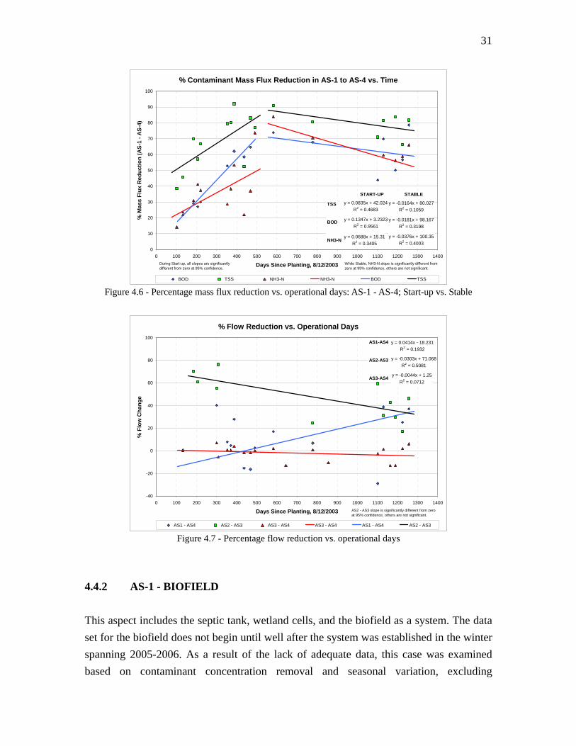
% Contaminant Mass Flux Reduction in AS-1 to AS-4 vs. Time
y = 0.0688x + 15.31R2 = 0.3405
y = 0.1347x + 3.2323R2 = 0.9561
y = 0.0835x + 42.024R2 = 0.4683
y = -0.0181x + 98.167R2 = 0.3198
y = -0.0164x + 80.027R2 = 0.1059
y = -0.0376x + 100.35R2 = 0.4003
0
10
20
30
40
50
60
70
80
90
100
0 100 200 300 400 500 600 700 800 900 1000 1100 1200 1300 1400
Days Since Planting, 8/12/2003
% M
ass
Flux
Red
uctio
n (A
S-1
- AS-
4)
BOD TSS NH3-N NH3-N BOD TSS
TSS
BOD
NH3-N
START-UP STABLE
During Start-up, all slopes are significantly different from zero at 95% confidence.
While Stable, NH3-N slope is significantly different from zero at 95% confidence, others are not significant.
Figure 4.6 - Percentage mass flux reduction vs. operational days: AS-1 - AS-4; Start-up vs. Stable
% Flow Reduction vs. Operational Days
y = -0.0044x + 1.25R2 = 0.0712
y = 0.0414x - 18.231R2 = 0.1932
y = -0.0303x + 71.068R2 = 0.5081
-40
-20
0
20
40
60
80
100
0 100 200 300 400 500 600 700 800 900 1000 1100 1200 1300 1400
Days Since Planting, 8/12/2003
% F
low
Cha
nge
AS1 - AS4 AS2 - AS3 AS3 - AS4 AS3 - AS4 AS1 - AS4 AS2 - AS3
AS2 - AS3 slope is significantly different from zero at 95% confidence, others are not significant.
AS1-AS4
AS2-AS3
AS3-AS4
Figure 4.7 - Percentage flow reduction vs. operational days
4.4.2 AS-1 - BIOFIELD This aspect includes the septic tank, wetland cells, and the biofield as a system. The data set for the biofield does not begin until well after the system was established in the winter spanning 2005-2006. As a result of the lack of adequate data, this case was examined based on contaminant concentration removal and seasonal variation, excluding
32
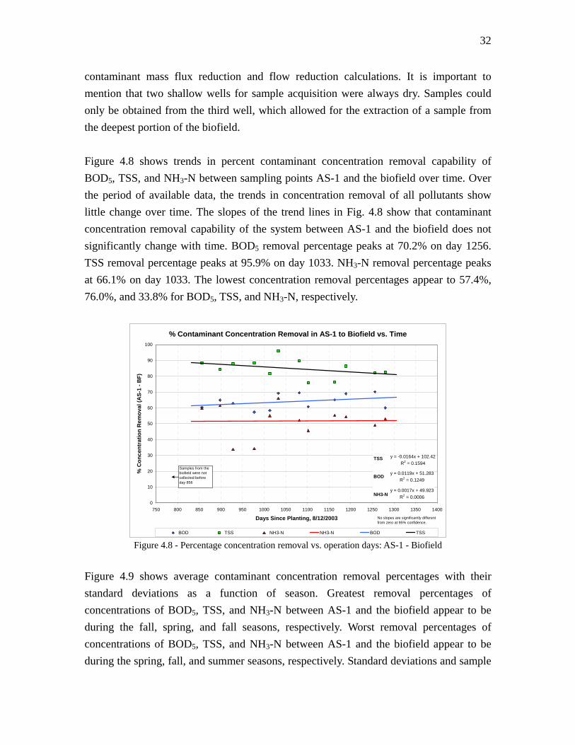
contaminant mass flux reduction and flow reduction calculations. It is important to mention that two shallow wells for sample acquisition were always dry. Samples could only be obtained from the third well, which allowed for the extraction of a sample from the deepest portion of the biofield. Figure 4.8 shows trends in percent contaminant concentration removal capability of BOD5, TSS, and NH3-N between sampling points AS-1 and the biofield over time. Over the period of available data, the trends in concentration removal of all pollutants show little change over time. The slopes of the trend lines in Fig. 4.8 show that contaminant concentration removal capability of the system between AS-1 and the biofield does not significantly change with time. BOD5 removal percentage peaks at 70.2% on day 1256. TSS removal percentage peaks at 95.9% on day 1033. NH3-N removal percentage peaks at 66.1% on day 1033. The lowest concentration removal percentages appear to 57.4%, 76.0%, and 33.8% for BOD5, TSS, and NH3-N, respectively.
% Contaminant Concentration Removal in AS-1 to Biofield vs. Time
y = 0.0017x + 49.923R2 = 0.0006
y = 0.0119x + 51.283R2 = 0.1249
y = -0.0164x + 102.42R2 = 0.1594
0
10
20
30
40
50
60
70
80
90
100
750 800 850 900 950 1000 1050 1100 1150 1200 1250 1300 1350 1400
Days Since Planting, 8/12/2003
% C
once
ntra
tion
Rem
oval
(AS-
1 - B
F)
BOD TSS NH3-N NH3-N BOD TSS
No slopes are significantly different from zero at 95% confidence.
TSS
BOD
NH3-N
Samples from the biofield were not collected before day 856
Figure 4.8 - Percentage concentration removal vs. operation days: AS-1 - Biofield
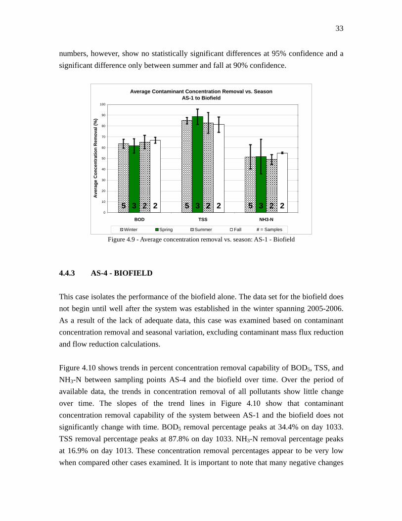
Figure 4.9 shows average contaminant concentration removal percentages with their standard deviations as a function of season. Greatest removal percentages of concentrations of BOD5, TSS, and NH3-N between AS-1 and the biofield appear to be during the fall, spring, and fall seasons, respectively. Worst removal percentages of concentrations of BOD5, TSS, and NH3-N between AS-1 and the biofield appear to be during the spring, fall, and summer seasons, respectively. Standard deviations and sample
33
numbers, however, show no statistically significant differences at 95% confidence and a significant difference only between summer and fall at 90% confidence.
Average Contaminant Concentration Removal vs. SeasonAS-1 to Biofield
5 5 53 3 32 2 22 2 20
10
20
30
40
50
60
70
80
90
100
BOD TSS NH3-N
Ave
rage
Con
cent
ratio
n R
emov
al (%
)
0
10000
20000
30000
40000
50000
60000
70000
80000
90000
100000
Winter Spring Summer Fall Series5# = Samples Figure 4.9 - Average concentration removal vs. season: AS-1 - Biofield
4.4.3 AS-4 - BIOFIELD This case isolates the performance of the biofield alone. The data set for the biofield does not begin until well after the system was established in the winter spanning 2005-2006. As a result of the lack of adequate data, this case was examined based on contaminant concentration removal and seasonal variation, excluding contaminant mass flux reduction and flow reduction calculations. Figure 4.10 shows trends in percent concentration removal capability of BOD5, TSS, and NH3-N between sampling points AS-4 and the biofield over time. Over the period of available data, the trends in concentration removal of all pollutants show little change over time. The slopes of the trend lines in Figure 4.10 show that contaminant concentration removal capability of the system between AS-1 and the biofield does not significantly change with time. BOD5 removal percentage peaks at 34.4% on day 1033. TSS removal percentage peaks at 87.8% on day 1033. NH3-N removal percentage peaks at 16.9% on day 1013. These concentration removal percentages appear to be very low when compared other cases examined. It is important to note that many negative changes
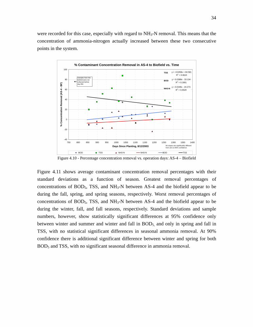
34
were recorded for this case, especially with regard to NH3-N removal. This means that the concentration of ammonia-nitrogen actually increased between these two consecutive points in the system.
% Contaminant Concentration Removal in AS-4 to Biofield vs. Time
y = 0.0199x - 24.273R2 = 0.0529
y = 0.0388x - 33.134R2 = 0.1661
y = -0.0458x + 84.581R2 = 0.0615
-40
-20
0
20
40
60
80
100
750 800 850 900 950 1000 1050 1100 1150 1200 1250 1300 1350 1400
Days Since Planting, 8/12/2003
% C
once
ntra
tion
Rem
oval
(AS-
4 - B
F)
BOD TSS NH3-N NH3-N BOD TSS
No slopes are significantly different from zero at 95% confidence.
TSS
BOD
NH3-N
Samples from the biofield were not collected before day 856
Figure 4.10 - Percentage concentration removal vs. operation days: AS-4 – Biofield
Figure 4.11 shows average contaminant concentration removal percentages with their standard deviations as a function of season. Greatest removal percentages of concentrations of BOD5, TSS, and NH3-N between AS-4 and the biofield appear to be during the fall, spring, and spring seasons, respectively. Worst removal percentages of concentrations of BOD5, TSS, and NH3-N between AS-4 and the biofield appear to be during the winter, fall, and fall seasons, respectively. Standard deviations and sample numbers, however, show statistically significant differences at 95% confidence only between winter and summer and winter and fall in BOD5, and only in spring and fall in TSS, with no statistical significant differences in seasonal ammonia removal. At 90% confidence there is additional significant difference between winter and spring for both BOD5 and TSS, with no significant seasonal difference in ammonia removal.

35
Average Contaminant Concentration Removal vs. SeasonAS-4 to Biofield
5 5 53 3 32 2 22 2 2-40
-20
0
20
40
60
80
100
BOD TSS NH3-N
Ave
rage
Con
cent
ratio
n R
emov
al (%
)
0
10000
20000
30000
40000
50000
60000
70000
80000
90000
100000
Winter Spring Summer Fall Series5# = Samples Figure 4.11 - Average concentration removal vs. season: AS-4 - Biofield
4.4.4 SURGE TANK - BIOFIELD With the inclusion of the surge tank, this case could examine the entire system. The surge tank was installed in the summer of 2006 to help eliminate peak flows into the wetland system and to help stabilize flow patterns. The data set for the biofield does not begin until the winter spanning 2005-2006. The data set for the surge tank begins in the fall of 2006. As a result of the lack of adequate data, this case was examined based on contaminant concentration removal and seasonal variation, excluding contaminant mass flux reduction and flow reduction calculations. Figure 4.12 shows trends in percent concentration removal capability of BOD5, TSS, and NH3-N between the surge tank and the biofield over time. Over the period of available data, the trends in concentration removal of all pollutants show little change over time. The slopes of the trend lines in Fig 4.12 show that contaminant concentration removal capability of the system between the surge tank and the biofield does not significantly change with time. However, strong conclusions cannot be drawn as the data is too sparse. Average removal percentage of BOD5, TSS, and NH3-N are 72.1%, 85.7%, and 42.6%, respectively. Because there are only four data points for this analysis, high and low values do not disclose enough information. However, the standard deviations for these values are also very small, all under 6.5%. It is important to note, again, that these values are based on a limited amount of data and only during a period after system establishment.
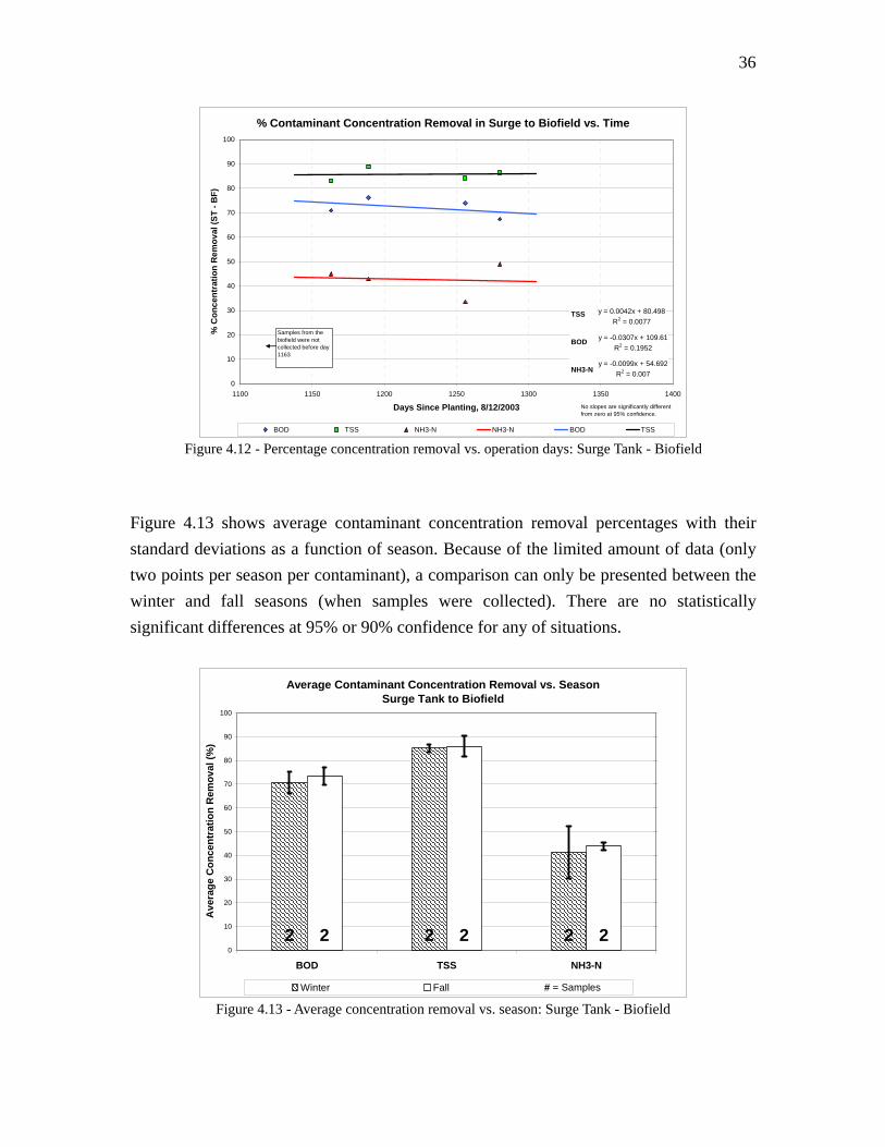
36
% Contaminant Concentration Removal in Surge to Biofield vs. Time
y = -0.0099x + 54.692R2 = 0.007
y = -0.0307x + 109.61R2 = 0.1952
y = 0.0042x + 80.498R2 = 0.0077
0
10
20
30
40
50
60
70
80
90
100
1100 1150 1200 1250 1300 1350 1400
Days Since Planting, 8/12/2003
% C
once
ntra
tion
Rem
oval
(ST
- BF)
BOD TSS NH3-N NH3-N BOD TSS
No slopes are significantly different from zero at 95% confidence.
TSS
BOD
NH3-N
Samples from the biofield were not collected before day 1163
Figure 4.12 - Percentage concentration removal vs. operation days: Surge Tank - Biofield
Figure 4.13 shows average contaminant concentration removal percentages with their standard deviations as a function of season. Because of the limited amount of data (only two points per season per contaminant), a comparison can only be presented between the winter and fall seasons (when samples were collected). There are no statistically significant differences at 95% or 90% confidence for any of situations.
Average Contaminant Concentration Removal vs. SeasonSurge Tank to Biofield
2 2 22 2 20
10
20
30
40
50
60
70
80
90
100
BOD TSS NH3-N
Ave
rage
Con
cent
ratio
n R
emov
al (%
)
0
10000
20000
30000
40000
50000
60000
70000
80000
90000
100000
Winter Fall Series5# = Samples Figure 4.13 - Average concentration removal vs. season: Surge Tank - Biofield
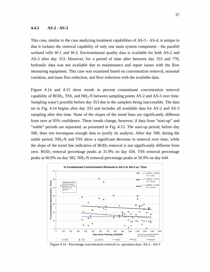
37
4.4.5 AS-2 - AS-3 This case, similar to the case analyzing treatment capabilities of AS-3 - AS-4, is unique in that it isolates the removal capability of only one main system component - the parallel wetland cells W-1 and W-2. Environmental quality data is available for both AS-2 and AS-3 after day 353. However, for a period of time after between day 353 and 778, hydraulic data was not available due to maintenance and repair issues with the flow measuring equipment. This case was examined based on concentration removal, seasonal variation, and mass flux reduction, and flow reduction with the available data. Figure 4.14 and 4.15 show trends in percent contaminant concentration removal capability of BOD5, TSS, and NH3-N between sampling points AS-2 and AS-3 over time. Sampling wasn’t possible before day 353 due to the samplers being inaccessible. The data set in Fig. 4.14 begins after day 353 and includes all available data for AS-2 and AS-3 sampling after this time. None of the slopes of the trend lines are significantly different from zero at 95% confidence. These trends change, however, if data from “start-up” and “stable” periods are separated, as presented in Fig. 4.15. The start-up period, before day 500, does not encompass enough data to justify its analysis. After day 500, during the stable period, NH3-N and TSS show a significant decrease in removal over time, while the slope of the trend line indicative of BOD5 removal is not significantly different from zero. BOD5 removal percentage peaks at 31.9% on day 436. TSS removal percentage peaks at 60.9% on day 582. NH3-N removal percentage peaks at 56.9% on day 644.
% Contaminant Concentration Removal in AS-2 to AS-3 vs. Time
y = -0.0002x + 15.023R2 = 2E-05
y = -0.0044x + 29.325R2 = 0.012
y = -0.0065x + 21.685R2 = 0.0219
0
10
20
30
40
50
60
70
0 100 200 300 400 500 600 700 800 900 1000 1100 1200 1300 1400
Days Since Planting, 8/12/2003
% C
once
ntra
tion
Rem
oval
(AS-
2 - A
S-3)
BOD TSS NH3-N BOD TSS NH3-N
No slopes are significantly different from zero at 95% confidence.
TSS
BOD
NH3-N
Samples from AS-3 were not collected available prior to day 353 due to lock problems
Figure 4.14 - Percentage concentration removal vs. operation days: AS-2 - AS-3

38
% Contaminant Concentration Removal in AS-2 to AS-3 vs. Time
y = -0.0269x + 53.317R2 = 0.2469
y = -0.0192x + 34.949R2 = 0.2857
y = -0.03x + 47.635R2 = 0.1946
0
10
20
30
40
50
60
70
300 400 500 600 700 800 900 1000 1100 1200 1300 1400
Days Since Planting, 8/12/2003
% C
once
ntra
tion
Rem
oval
(AS-
2 - A
S-3)
BOD TSS NH3-N TSS BOD NH3-N
While stable, only BOD5 slope is not significantly different from zero at 95% confidence, others are
TSS
BOD
NH3-N
STABLESamples from AS-3 were not collected available prior to day 353 due to lock problems
Figure 4.15 - Percentage concentration removal vs. operation days: AS-2 - AS-3; Start-up vs. Stable
Figure 4.16 shows average concentration removal percentages with their standard deviations as a function of season. Greatest removal percentages of concentrations of BOD5, TSS, and NH3-N between AS-2 and AS-3 appear to be during the fall, spring, and spring seasons, respectively. Worst removal percentages of concentrations of BOD5, TSS, and NH3-N between AS-2 and AS-3 appear to be during the summer, winter, and winter seasons, respectively. Standard deviations and sample numbers, however, show the only statistically significant difference at 95% confidence between winter and summer in NH3-N, with no statistical significant differences in seasonal BOD5 or TSS removal, and no significant differences at 90% confidence. Figure 4.17 shows percentage changes in contaminant mass flux between AS-2 and AS-3 over time. No data points before day 778 are available due to the unavailable environmental data before day 353 and unavailable hydraulic data between days 353 and 778. Thus, the available data falls within the “stable” period of the wetland. None of the slopes of the trend lines in Fig. 4.17 are significantly different from zero. The highest values of percentage removal of mass flux for BOD5, TSS, and NH3-N for this case are 79.4%, 77.9%, and 98.3%, respectively. It is important to note, however, that the variance in the BOD5 and TSS data points is fairly significant, as the lowest values fall to 12.4% for TSS and 1.2% for BOD5. These low values are present within the last year of sampling.

39
Average Contaminant Concentration Removal vs. SeasonAS-2 to AS-3
6 6 55 5 53 5 56 5 6-20
-10
0
10
20
30
40
50
60
70
80
BOD TSS NH3-N
Ave
rage
Con
cent
ratio
n R
emov
al (%
)
0
10000
20000
30000
40000
50000
60000
70000
80000
90000
100000
Winter Spring Summer Fall Series5# = Samples Figure 4.16 - Average concentration removal vs. season: AS-2 - AS-3
% Contaminant Mass Flux Reduction in AS-2 to AS-3 vs. Time
y = 0.0027x + 41.332R2 = 0.0005
y = 0.015x + 28.416R2 = 0.0305
y = -0.016x + 72.187R2 = 0.0387
0
10
20
30
40
50
60
70
80
700 800 900 1000 1100 1200 1300 1400
Days Since Planting, 8/12/2003
% M
ass
Flux
Red
uctio
n (A
S2 -
AS3
)
BOD TSS NH3-N NH3-N BOD TSS
TSS
BOD
NH3-N
No slopes are significantly different from zero at 95% confidence.
Flow monitoring equipment was damaged for a period of time before day 778, prior to which samples from AS-3 were not collected due to lock problems.
Flow was shut off to the system for a period of time before after day 778
Figure 4.17 - Percentage mass flux reduction vs. operational days: AS-2 - AS-3
Figure 4.7 shows flow reduction capability between AS-2 and AS-3 over time. Hydraulic data between days 353 and 778 was unavailable. However, the available data spans both the start-up and stable periods of the lifetime of the wetland system. The slope of the best fit line through the available data is significantly different from zero, indicating that flow reduction capability over time decreased in this case. The highest amount of flow reduction was recorded on day 308, where 76.4% of the flow was reduced; the lowest flow reduction was recorded on day 1225, where 16.9% of the flow was reduced.

40
4.4.6 AS-3 - AS-4 This case, similar to the case analyzing treatment capabilities of AS-2 - AS-3, isolates the removal capability of only one main system component - the “polishing” wetland cell W-3. Much data is available for AS-3 and AS-4, as sampling from these stations began at the earliest stages of research. However, for a period of time before day 353, environmental quality data was not available. This case was examined based on concentration removal, seasonal variation, and mass flux reduction, and flow reduction with the available data. Figures 4.18 and 4.19 show trends in percent contaminant concentration removal capability of BOD5, TSS, and NH3-N between sampling points AS-3 and AS-4 over time. Sampling wasn’t possible before day 353 due to the samplers being inaccessible. The data set in Fig. 4.18 begins after day 353 and includes all available data for AS-3 and AS-4 sampling after this time. The slopes of the trend lines in Fig. 4.18 show that, over the period of time encompassing the “start-up” and “stable” periods, BOD5 and NH3-N concentration removal capability is significant and increases over time, while TSS removal does not significantly change. These trends change, however, if data from start-up and stable periods are separated, as presented in Fig. 4.19. The start-up period, before day 500, does not encompass enough data to justify its analysis. After day 500, during the stable period, only BOD5 shows a significant increase in removal over time, while slopes of trend lines indicative of NH3-N and TSS removal are not significantly different from zero. BOD5 removal percentage peaks at 44.2% on day 1163. TSS removal percentage peaks at 85.2% on day 469. NH3-N removal percentage peaks at 41.8% on day 674. Figure 4.20 shows average contaminant concentration removal percentages with their standard deviations as a function of season. Greatest removal percentages of concentrations of BOD5, TSS, and NH3-N between AS-2 and AS-3 appear to be during the fall, spring, and spring seasons, respectively. Worst removal percentages of concentrations of BOD5, TSS, and NH3-N between AS-2 and AS-3 appear to be during the summer, winter, and winter seasons, respectively. Standard deviations and sample numbers, however, show the only statistically significant difference at 95% confidence between winter and summer in NH3-N, with no statistical significant differences in seasonal BOD5 or TSS removal, and no significant differences at 90% confidence.

41
% Contaminant Concentration Removal in AS-3 to AS-4 vs. Time
y = 0.0138x + 18.311R2 = 0.1823
y = -0.0076x + 55.567R2 = 0.019
y = 0.0312x - 9.0289R2 = 0.4559
-20
-10
0
10
20
30
40
50
60
70
80
0 100 200 300 400 500 600 700 800 900 1000 1100 1200 1300 1400
Days Since Planting, 8/12/2003
% C
once
ntra
tion
Rem
oval
(AS-
3 - A
S-4)
BOD TSS NH3-N BOD TSS NH3-N
TSS
BOD
NH3-N
Only TSS slope is not significantly different from zero at 95% confidence, all others are significant.
Samples from AS-3 were not collected available prior to day 353 due to lock problems
Figure 4.18 - Percentage concentration removal vs. operation days: AS-3 - AS-4
% Contaminant Concentration Removal in AS-3 to AS-4 vs. Time
y = -0.0085x + 56.351R2 = 0.0176
y = 0.0311x - 0.1599R2 = 0.4996
y = 0.0036x + 21.263R2 = 0.0034
-10
0
10
20
30
40
50
60
70
80
90
250 350 450 550 650 750 850 950 1050 1150 1250 1350
Days Since Planting, 8/12/2003
% C
once
ntra
tion
Rem
oval
(AS-
3 - A
S-4)
BOD TSS NH3-N TSS BOD NH3-N
TSS
BOD
NH3-N
STABLE
While stable, BOD slope is significantly different from zero at 95% confidence, all others are not significant.
Figure 4.19 - Percentage concentration removal vs. operation days: AS-3 - AS-4; Start-up vs. Stable
Figures 4.21 and 4.22 shows percentage changes in contaminant mass flux between AS-3 and AS-4 over time. The slopes of the trend lines in Fig. 4.21 show that, over the period of time encompassing the “start-up” and “stable” periods, no change in mass flux reduction capability is significant at 95% confidence. These trends are the same if data from the only the stable period (after day 500) is analyzed, as presented in Fig. 4.22. The highest values of percentage removal of mass flux for BOD5, TSS, and NH3-N for this case are 78.7%, 92.0%, and 83.9%, respectively. The lowest values all fall below 25%.
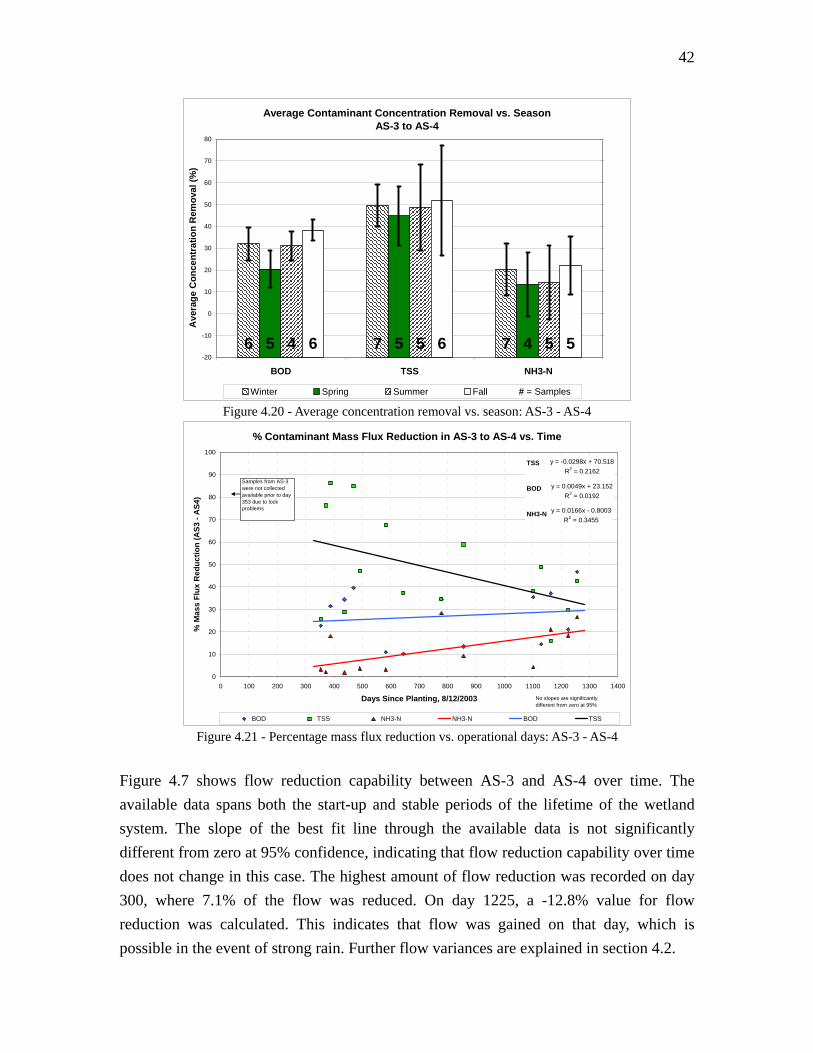
42
Average Contaminant Concentration Removal vs. SeasonAS-3 to AS-4
6 7 75 5 44 5 56 6 5-20
-10
0
10
20
30
40
50
60
70
80
BOD TSS NH3-N
Ave
rage
Con
cent
ratio
n R
emov
al (%
)
0
10000
20000
30000
40000
50000
60000
70000
80000
90000
100000
Winter Spring Summer Fall Series5# = Samples Figure 4.20 - Average concentration removal vs. season: AS-3 - AS-4
% Contaminant Mass Flux Reduction in AS-3 to AS-4 vs. Time
y = 0.0166x - 0.8003R2 = 0.3455
y = 0.0049x + 23.152R2 = 0.0192
y = -0.0298x + 70.518R2 = 0.2162
0
10
20
30
40
50
60
70
80
90
100
0 100 200 300 400 500 600 700 800 900 1000 1100 1200 1300 1400
Days Since Planting, 8/12/2003
% M
ass
Flux
Red
uctio
n (A
S3 -
AS4
)
BOD TSS NH3-N NH3-N BOD TSS
TSS
BOD
NH3-N
No slopes are significantly different from zero at 95%
Samples from AS-3 were not collected available prior to day 353 due to lock problems
Figure 4.21 - Percentage mass flux reduction vs. operational days: AS-3 - AS-4
Figure 4.7 shows flow reduction capability between AS-3 and AS-4 over time. The available data spans both the start-up and stable periods of the lifetime of the wetland system. The slope of the best fit line through the available data is not significantly different from zero at 95% confidence, indicating that flow reduction capability over time does not change in this case. The highest amount of flow reduction was recorded on day 300, where 7.1% of the flow was reduced. On day 1225, a -12.8% value for flow reduction was calculated. This indicates that flow was gained on that day, which is possible in the event of strong rain. Further flow variances are explained in section 4.2.

43
% Contaminant Mass Flux Reduction in AS-3 to AS-4 vs. Time
y = 0.0104x + 3.0231R2 = 0.0479
y = 0.0318x - 5.9852R2 = 0.3615
y = -0.0304x + 70.981R2 = 0.2602
-10
0
10
20
30
40
50
60
70
80
0 100 200 300 400 500 600 700 800 900 1000 1100 1200 1300 1400
Days Since Planting, 8/12/2003
% M
ass
Flux
Red
uctio
n (A
S3 -
AS4
)
BOD TSS NH3-N NH3-N BOD TSS
No slopes are significantly different from zero at 95% confidence.
TSS
BOD
NH3-N
STABLE
Samples from AS-3 were not collected available prior to day 353 due to lock problems
Figure 4.22 - Percentage mass flux reduction vs. operational days: AS-3 - AS-4; Start-up vs. Stable
4.5 WETLAND PLANTS ANALYSIS The subsurface wetland cells of the system in Greenfield were originally planted with about 13 species of plants (Table 4.5), totaling about 4,000 plants within all cells. All species were planted in a randomly mixed fashion throughout all of the wetland cells. Of these species, observations over the lifetime of the system have shown many of the species to become extinct. After the first winter (2003-04) some of the species planted did not grow in the following blooming season. After the subsequent winter (2004-05), a greater number of invasive species were found in the places of the missing wetland plants, and in the spring of 2006, many invasive species were found mixed with the few wetland species remaining to date. Wetland plants are essential to the treatment capabilities of the system, owing to their aptitude for providing oxygen to the bacteria that live in the root zone and also as agents of evapotranspiration. Since the original construction of the system, completed in August of 2003, the wetlands have undergone much change with regard to plant media presence, particularly within the parallel wetland cells W-1 and W-2. As the system was modified and upgraded, variability in water flow rate put additional stress on the wetland plants. Many of the species died and/or have been replaced by invasive species. Figure 4.23
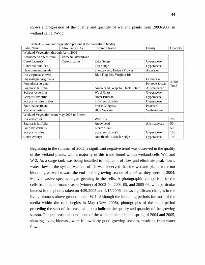
44
shows a progression of the quality and quantity of wetland plants from 2003-2006 in wetland cell 1 (W-1). Table 4.5 - Wetland vegetation present at the Greenfield facility.
Latin Name Also Known As Common Name Family QuantityWetland Vegetation through April 2006 Actinomeris alternifolia Verbesin alternifolia Carex lacustris Carex riparias Lake Sedge Cyperaceae Carex vulpinoidea Fox Sedge Cyperaceae Helenium autumnale Sneezeweed, Helen's Flower Asteracea Iris virginica shrevei Blue Flag Iris, Virginia Iris Physostegia virginiana Lamiaceae Pontederia cordata PontederiaceaeSagittaria latifolia Arrowhead, Wapato, Duck Potato Alismataceae Scirpus cyperinus Wool Grass Cyperaceae Scirpus fluviatilis River Bulrush Cyperaceae Scirpus validus creber Softstem Bulrush Cyperaceae Spartina pectinata Prarie Codgrass Poaceae Verbena hastate Blue Vervain Verbenaceae
4,000 Total
Wetland Vegetation from May 2006 to Present Iris versicolor Wild Iris 200 Sagittaria latifolia Arrowhead Alismataceae 50 Saururus cernuus Lizard's Tail 50 Scirpus validus Softstem Bulrush Cyperaceae 100 Carex emoryi Riverbank Russock Sedge Cyperaceae 100
Beginning in the summer of 2005, a significant negative trend was observed in the quality of the wetland plants, with a majority of this trend found within wetland cells W-1 and W-2. As a surge tank was being installed to help control flow and eliminate peak flows, water flow to the system was cut off. It was observed that the wetland plants were not blooming as well toward the end of the growing season of 2005 as they were in 2004. Many invasive species began growing in the cells. A photographic comparison of the cells from the dormant season (winter) of 2003-04, 2004-05, and 2005-06, with particular interest in the photos taken on 4/29/2005 and 4/15/2006, shows significant changes in the living biomass above ground in cell W-1. Although the blooming periods for most of the media within the cells begins in May (New, 2006), photographs of the short period preceding the start of the seasonal bloom indicate the quality and quantity of the growing season. The pre-seasonal conditions of the wetland plants in the spring of 2004 and 2005, showing living biomass, were followed by good growing seasons, resulting from water flow.

45
Day 102
11/22/2003
Wetlands planted 08/12/2003 (Day 0) Planting in the latter portion of the
blooming season Minimal growth during remainder of
blooming season
Day 259
4/29/2004
Cold temperatures prevented growth and development during winter months
Plants look healthy and ready for spring bloom
Some species are no longer present
Day 298
6/07/2004
Seasonal warmth and adequate water and nutrients allow vast growth
Some invasive species are present in the wetland cells
Day 434
10/21/2004
End of growing season is approaching Plants are unhealthy due to lack of
steady water flow
Day 674
6/17/2005
Plants flourish after winter season More species are no longer present Invasive species have increased
Day 777
9/28/2005
Flow was minimal/inconsistent during surge tank installation
Plants began dying earlier in this growing season than the previous year
Many dead plants and invasive species were pulled out of the wetland
Day 975
4/15/2006
Many wetland plants are missing Pre-blooming season inspection shows
much worse condition of plant media this season than the last
Figure 4.23 - Growth progression of wetland plants in wetland cell 1 (W-1)

46
As a result of the loss of many of the wetland plants that were originally implemented into the wetland cells, the wetlands were replanted with an assortment of five different wetland species in the spring of 2006. A comparison of the vegetation present in the wetlands before and after the replanting can be seen in Table 4.5. The Carex lacustris and Carex vulpinoidea species (sedges) were appended with a different sedge species, Carex emoryi. The arrowhead species was not changed, retaining Sagittaria latifolia. One of the bulrush species was also replenished with the same species, Scirpus validus. The original iris species, Iris virginica shrevei, was satiated with a similar breed, Iris versicolor. In addition to the reintroduction of some of the familiar species, a new variety of plant was introduced into the system; Saururus cernuus, more commonly known as lizard’s tail. Plants belonging to the family of this species were not used in any of the cases examined within the literature review. Supplementing the wetlands with these five wetland species was a much needed face-lift for the system, as the bare patches and weed-laden areas were beginning to comprise the majority of wetland area. However, the replanting of the cells has two significant drawbacks with regard to the pollutant removal method and capability of the system. First, it is anticipated that the immature plants in the system will need time to fully establish themselves in order to be able to have the capability of promoting the remediation of wastewater to a level as high as that of the fully mature plants within the system. When the wetland cells were originally planted in 2003, it took some time before the plants became fully established, and within that time period, concentration removal capability of the system was found to be weak, although steadily increasing as the plants matured and grew. Because plants have been proven to be significant promoters of treatment (as discussed in the literature review), their lack of performance due to immaturity may be reflected in the quality of the treated wastewater until they become established. Secondly, the planting scheme itself has changed; a variable that could have caused significant changes in treatment data since replanting. The wetland cells were replenished with just five new species, rather than a combination of the original thirteen. Also, most of the newly introduced plants were not the original species used. This could mean that some original species are or will soon become fully extinct within the wetlands. The literature that was reviewed proved that there were significant changes in treatment capability of a constructed wetland based on the types of plants used.

47
Throughout the study period, however, it was observed that the wetland plants found in the polishing wetland cell W-3 maintained their vitality for a longer amount of time than the plants found in cells W-1 and W-2. This wetland cell was also observed to have much less loss of wetland plants and fewer invasive species growing with the cell. Although a complete photographic timeline is not available of wetland cell W-3, Figure 4.24 exhibits the cell in the summer of 2005.
Figure 4.24 - Wetland cell W-3
48
CHAPTER 5
CONCLUSIONS AND LESSONS LEARNED 5.1 CONTAMINANT CONCENTRATION REMOVAL CONCLUSIONS Before the conclusions are discussed it is important to note that, even with reductions in contaminants, the effluent wastestream did not meet surface and subsurface discharges regulations (see Table 1.2). As was mentioned previously, the wetland system in this study differs from many other studies in having unusually high loading rates and extreme variability in flow rates. However, overall performance was not atypical of other studies. 5.1.1 SYSTEM-BASED PERFORMANCE Percent concentration removal statistics for the cases examined yield a number of noteworthy conclusions. The cases examined can be divided into two categories. The first category includes cases that describe system performance, where the system includes multiple components. These cases include the examination of AS-1 - AS-4, AS-1 - Biofield, and Surge Tank - Biofield. The system-based cases are then examined based on individual contaminants. With regard to BOD5 removal capability based on percentage concentration reduction, examining all data, the data shows that the best removal occurs system-wide with the surge tank and biofield (case ST - BF, Table 4.1), where the average removal percentage is 72.1%. However, this conclusion is based on only four data points. The next highest removal percentage is in the case of AS-1 - Biofield, where the average is 64.0%. (12 data points) The case of AS-1 - AS-4, containing the largest pool of data points, has an average removal percentage of 55.8%. Overall the wetland cells appear to be contributing to BOD5 removal. With regard to TSS removal capability based on percentage concentration reduction, examining all data, the data shows trends very similar to that of BOD5 removal capability. The best removal occurs system-wide with the surge tank and biofield (case ST - BF,

49
Table 4.2), where the average removal percentage is 85.7%. However, this is based on only four data points. The next highest removal percentage is in the case of AS-1 - Biofield, where the average is 85.0%. (12 data points) The case of AS-1 - AS-4, with the largest pool of data points, has an average removal percentage of 73.3%. With regard to NH3-N removal capability based on percentage concentration reduction, trends are different from that of BOD5 and TSS. Examining all data, the data shows that the best removal occurs system-wide with the AS1 - Biofield case (Table 4.3), where the average removal percentage is 51.8%, based on only 12 data points. The next highest removal percentage is in the case of AS-1 - AS-4 (containing the largest pool of data points), where the average is 47.2%. The case of the surge tank - biofield had a removal capability of 42.6%, based on just four data points. Looking at system-wide performance, taking into account all data, the best performance overall appears to lie within systems that have the most treatment components as would be expected. The case of AS-1 - AS-4 effectively describes treatment from three wetland system components at Greenfield - the second septic tank ST-2, the parallel wetland cells W-1 and W-2, and the polishing cell W-3. The other two systems described include those components as well as a biofield (AS-1 - Biofield) or a surge tank (Surge Tank - Biofield). These larger systems tend to perform better in terms of percent concentration removal of contaminants. 5.1.2 COMPONENT-BASED PERFORMANCE Three of the cases examined lead to component-based conclusions following data analysis. The case of AS-2 - AS-3 isolates the parallel wetland cells W-1 and W-2. This system component can be compared to the case of AS-3 - AS-4, which isolates the polishing wetland cell W-3, and can also be compared to the treatment capability of the biofield in the case of AS-4 - Biofield. With regard to BOD5 removal capability based on percentage concentration reduction, examining all data, the data shows that the best component-based removal occurs within the case of AS-3 - AS-4, which essentially is the third polishing wetland cell. On average this component removed 30.9% of BOD5. The parallel wetland cells, case AS-2 - AS-3, had the next best average removal percentage, 14.8%. The worst percent removal
50
capability of BOD5 was through the biofield, case AS-4 - Biofield, where the average removal percentage was 8.2%. It is also important to note that this case also had a negative minimum removal value of -11.2%, which signifies deterioration in water quality based on BOD5 concentration. With regard to TSS removal capability based on percentage concentration reduction, trends are slightly different from that of BOD5. Examining all data, the data shows that the best removal by component occurs in the case of AS-3 - AS-4, the third wetland cell, where the average removal percentage is 49.0%. The next highest removal percentage is in the case of the biofield, AS-4 - Biofield, where the average is 35.8%. It is also important to note that this case also had a negative minimum removal value of -6.9%, which signifies a worsening in water quality based on TSS concentration. In the case of AS-2 - AS-3, the parallel wetland cells had a removal capability of 25.4%, but no negative minimum values. With regard to NH3-N removal capability based on percentage concentration reduction, the data shows trends very similar to that of BOD5 removal capability. The data shows that the best component-based removal occurs within the case of AS-3 - AS-4, the third polishing wetland cell (refer to Table 4.3). On average this component removed 18.0% of NH3-N. The parallel wetland cells, case AS-2 - AS-3, had the next best average removal percentage, 16.1%. The worst percent removal capability of NH3-N was through the biofield, case AS-4 - Biofield, where the average removal percentage itself was negative (-3.1%). The lowest minimum value was as low as -23.7%. This signifies a worsening in water quality based on NH3-N concentration. These results show, based on average percent concentration removal statistics, that the sand mound biofield has the worst performance of all of the examined individual wetland system components. Not only were removal capabilities of the biofield minimal in BOD5 and TSS removal, they were adverse in the removal capability of NH3-N. The biofield actually causes the concentration of ammonia-nitrogen to increase if it is used as a component in the treatment system. These results could be explained in a few ways. First, the biofield receives a limited amount of flow through it (400 gallons per day, by design). The lack of flow may not allow for the sustenance of bacteria within the biofield to perform the necessary work in pollutant removal. Second, it is important to consider that the non-wetland vegetation that

51
grows atop the sand mound. These plants and grasses must uptake water for their survival. If water is removed by plant uptake and evaporation at a rate greater than the rate of nutrient removal by physical, chemical, or biological processes, the concentration of contaminants in the water will increase. Examining component-based performance, the best average percent concentration removal overall is seen in the case of AS-3 - AS-4, the third wetland cell W-3. When compared to the other cases discussing component-based performance, these results show that there is most improvement when using a polishing wetland cell, based on average percentage concentration reduction. 5.1.3 SYSTEMS OF COMBINED COMPONENTS VS. INDIVIDUAL
COMPONENTS In addition to the conclusions drawn from the examination of three cases comparing systems of components and the examination of three cases comparing individual components, conclusions can also be drawn when comparing the general performance of systems of components versus individual components used to treat wastewater. Considering the average contaminant concentration removal capabilities of systems of components of all contaminants seen in Table 5.1, 5.2, and 5.3, and comparing these average values to those of the removal capabilities of the individual components, it can be seen that contaminant concentration reduction is best with a system of components. The use of more components within a wetland system for the treatment of wastewater results in better contaminant concentration removal. 5.1.4 START-UP VS. STABLE PERIODS Analysis of trends in contaminant concentration removal data shows a number of data sets that have best fit trend slopes significantly different from zero at 95% confidence. These significant slopes mean that the change in contaminant concentration removal capability over time is significant. The trend lines seen through data in Fig. 4.2, displaying percent contaminant concentration removal in AS-1 - AS-4 over time, have significant positive slopes in the case of BOD5 and NH3-N removal, while the slope for TSS removal is not significant. When hypothetical start-up data is separated from the

52
remaining data, all trends have significant slopes, and all slope values are greater than those from the data set representing all data. The data from the hypothetical stable period in Fig. 4.3 shows no positive significant slopes for the trend lines. Additionally, similar trends are found in contaminant mass flux reduction. These findings support the claim of a distinct start-up period during the first year of plant establishment, followed by a period of stable system performance. Table 5.1 - Percent concentration removal statistics: BOD BOD5 AS1-AS4 AS1-BF AS4-BF ST-BF AS2-AS3 AS3-AS4
Data Pts. 26 12 12 4 20 21 Average 55.8 64.0 8.2 72.1 14.8 30.9 Maximum 69.7 70.2 34.4 76.2 31.9 44.2 Minimum 23.2 57.4 -11.2 67.3 -23.9 8.9 A
ll D
ata
Std. Dev. 14.1 4.7 13.2 3.8 11.9 9.2 Data Pts. 9 5 5 2 6 6 Average 50.1 63.7 -1.7 70.6 17.6 32.0 Maximum 67.9 70.2 12.1 73.9 28.2 43.1 Minimum 23.2 60.1 -11.2 67.3 9.5 21.6 W
inte
r
Std. Dev. 18.5 4.2 9.3 4.6 7.7 7.4 Data Pts. 6 3 3 0 5 5 Average 54.7 61.7 17.2 --- 15.9 20.5 Maximum 69.4 69.3 34.4 --- 26.2 30.7 Minimum 30.0 57.4 2.9 --- 3.9 8.9 Sp
ring
Std. Dev. 14.4 6.6 15.9 --- 9.5 8.6 Data Pts. 5 2 2 0 3 4 Average 57.3 65.1 9.7 --- 4.6 31.0 Maximum 67.6 69.5 9.8 --- 23.4 37.1 Minimum 47.3 60.7 9.5 --- -23.9 22.0 Su
mm
er
Std. Dev. 9.5 6.2 0.2 --- 8.1 6.7 Data Pts. 6 2 2 2 6 6 Average 64.3 67.0 17.8 73.5 18.1 38.3 Maximum 69.7 69.0 26.1 76.2 31.9 44.2 Minimum 58.1 65.0 9.6 70.9 9.0 33.0
Fall
Std. Dev. 4.2 2.8 11.6 3.8 9.2 4.8 5.2 CONTAMINANT MASS FLUX REDUCTION CONCLUSIONS Percent contaminant mass flux reduction statistics for the cases examined yield several significant conclusions. First, two of the cases examined lead to component-based conclusions following data analysis. The case of AS-2 - AS-3 isolates the parallel wetland cells W-1 and W-2. This system component can be compared to the case of AS-3 - AS-4,

53
Table 5.2 - Percent concentration removal statistics: TSS TSS AS1-AS4 AS1-BF AS4-BF ST-BF AS2-AS3 AS3-AS4
Data Pts. 29 12 12 4 21 23 Average 73.3 85.0 35.8 85.7 25.4 49.0 Maximum 88.9 95.9 87.8 89.0 60.9 85.2 Minimum 38.5 76.0 -6.9 83.0 4.5 25.0 A
ll D
ata
Std. Dev. 12.4 5.7 25.6 2.7 12.1 16.8 Data Pts. 10 5 5 2 6 7 Average 69.2 85.1 35.6 85.3 19.6 49.6 Maximum 85.3 88.2 51.2 86.4 25.2 62.7 Minimum 45.5 82.1 20.0 84.2 16.3 38.2 W
inte
r
Std. Dev. 11.5 2.9 11.2 1.6 3.3 9.8 Data Pts. 6 3 3 0 5 5 Average 74.9 88.7 62.4 --- 29.8 44.8 Maximum 88.9 95.9 87.8 --- 60.9 66.7 Minimum 66.7 81.8 36.8 --- 14.1 30.1 Sp
ring
Std. Dev. 10.4 7.1 25.5 --- 19.2 13.6 Data Pts. 6 2 2 0 5 5 Average 81.5 82.8 19.0 --- 27.8 48.7 Maximum 88.9 89.6 44.8 --- 40.0 76.2 Minimum 77.5 76.0 -6.9 --- 4.5 25.0 Su
mm
er
Std. Dev. 4.4 9.6 36.6 --- 14.2 19.7 Data Pts. 7 2 2 2 5 6 Average 70.9 81.3 13.2 86.0 26.7 52.0 Maximum 86.4 86.4 26.3 89.0 40.5 85.2 Minimum 38.5 76.3 0.0 83.0 13.0 25.5
Fall
Std. Dev. 17.4 7.2 18.6 4.2 9.8 25.2 which isolates the polishing wetland cell W-3. With regard to BOD5 removal capability based on percent mass flux reduction, the data shows that the best component-based removal occurs within the case of the third polishing wetland cell (refer to Table 5.4). On average this component removed 61.9% of BOD5. The parallel wetland cells had an average removal percentage of 37.3%. With regard to TSS removal capability based on percent mass flux reduction, the data shows trends very similar to that of BOD5 removal capability. The data shows that the best component-based removal occurs within wetland cell W-3 (refer to Table 5.4). On average this component removed 70.4% of TSS. The parallel wetland cells had an average removal percentage of 41.7%. With regard to NH3-N removal capability based on percent mass flux reduction, trends are slightly different from that of BOD5 and TSS. Examining all data, it is observed that the best removal by component occurs in the case of AS-2 - AS-3, the parallel wetland cells, where the average removal percentage is 96.1%. In the case of the third wetland cell, AS-3 - AS-4, the average mass flux reduction is 54.6%.

54
Table 5.3 - Percent concentration removal statistics: NH3-N NH3-N AS1-AS4 AS1-BF AS4-BF ST-BF AS2-AS3 AS3-AS4
Data Pts. 12 12 4 4 21 21 Average 47.2 51.8 -3.1 42.6 16.1 18.0 Maximum 80.7 66.1 16.9 48.9 56.9 41.8 Minimum 14.3 33.8 -23.7 33.5 1.0 0.6 A
ll D
ata
Std. Dev. 16.3 9.9 12.0 6.5 13.4 14.1 Data Pts. 5 5 2 6 6 7 Average 48.8 51.5 -4.7 41.2 10.4 20.4 Maximum 73.0 61.7 5.7 48.9 19.7 36.9 Minimum 21.7 33.8 -17.0 33.5 4.2 3.4 W
inte
r
Std. Dev. 15.5 11.1 8.9 10.9 5.7 12.0 Data Pts. 3 3 0 5 5 4 Average 49.2 51.8 2.1 --- 22.7 16.7 Maximum 80.7 66.1 16.9 --- 56.9 35.4 Minimum 23.4 34.3 -16.7 --- 1.0 0.6 Sp
ring
Std. Dev. 20.2 16.1 17.1 --- 23.4 14.5 Data Pts. 2 2 0 3 4 5 Average 42.2 49.0 -2.0 --- 20.8 14.2 Maximum 60.0 52.3 2.5 --- 36.6 41.8 Minimum 22.6 45.7 -6.4 --- 11.4 1.5 Su
mm
er
Std. Dev. 13.5 4.6 6.3 --- 9.5 16.9 Data Pts. 2 2 2 6 6 5 Average 47.5 55.0 -8.1 43.9 14.7 26.2 Maximum 68.4 55.5 7.5 45.0 30.3 38.4 Minimum 14.3 54.6 -23.7 42.8 4.3 3.4
Fall
Std. Dev. 18.8 0.7 22.1 1.6 10.5 13.4 A strong conclusion cannot be reached with regard to which individual component performs better based percent contaminant mass flux reduction. It can be concluded that the polishing wetland cell W-3 does a better job of water treatment based on reduction of BOD5 and TSS. With the treatment of ammonia-nitrogen, however, the parallel wetland cell W-3 appears to be more effective. This conclusion could be explained by reasoning that cells W-1 and W-2 are immediately exposed to higher loading rates of ammonia and, as such, have the greatest opportunity for reduction of mass flux. Also, cells W-1 and W-2 do utilize a reciprocating draw and fill cycle that may in fact help introduce oxygen to the system quicker, in turn expediting the nitrification and denitrification processes. The cases examined include the case of AS-1 - AS-4, which describes a system that includes multiple components used for treatment, and compares the performance of this system to two cases that focus on the performance of individual components (the parallel wetland cells and the polishing wetland cell). With regard to the mass flux reduction

55
capability of BOD5, TSS, and NH3-N, the data shows in the case of AS-1 - AS-4 that the average mass flux removal percentages for the respective contaminants are 52.6%, 69.0%, and 46.0% (refer to Table 5.4). The average mass flux reduction capability of the parallel wetland cells (case AS-2 - AS-3) of the same contaminants are, respectively, 45.2%, 54.2%, and 44.0%. These average reductions are also lower for the polishing wetland cell (case AS-3 - AS-4), with reduction values being, respectively, 27.1%, 45.2%, and 9.6%. Based on this observation, a larger system proves to perform better in terms of percent contaminant mass flux reduction. This conclusion is concurrent with the conclusion reached following the analysis of percent contaminant concentration reduction in systems of components versus individual components. Table 5.4 - Percent mass flux reduction statistics
Percent Mass Flux Reduction AS1-AS4 AS2-AS3 AS3-AS4
Data Pts. 15 7 13 Average 52.6 45.2 27.1 Maximum 78.7 63.1 46.7 Minimum 23.6 24.8 10.2 B
OD
5
Std. Dev. 18.1 13.7 12.2 Data Pts. 19 7 15 Average 69.0 54.2 45.2 Maximum 92.0 75.6 86.3 Minimum 13.6 33.4 16.0
TSS
Std. Dev. 19.9 13.0 22.0 Data Pts. 18 7 14 Average 46.0 44.4 9.6 Maximum 83.9 74.2 28.3 Minimum 14.3 8.0 -2.6 N
H3-N
Std. Dev. 20.0 20.0 10.7
5.2.1 START-UP VS. STABLE PERIODS Analysis of trends in percent contaminant mass flux reduction data shows a number of data sets that have best fit trend slopes significantly different from zero at 95% confidence. These significant slopes mean that the change in contaminant mass flux reduction capability over time is significant. The trend lines seen through data in Fig 4.5, displaying percent contaminant mass flux reduction in AS-1 - AS-4 over time, have
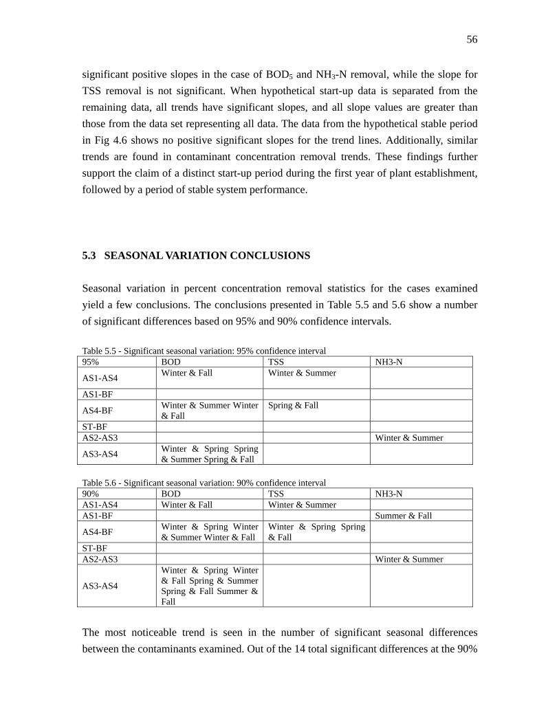
56
significant positive slopes in the case of BOD5 and NH3-N removal, while the slope for TSS removal is not significant. When hypothetical start-up data is separated from the remaining data, all trends have significant slopes, and all slope values are greater than those from the data set representing all data. The data from the hypothetical stable period in Fig 4.6 shows no positive significant slopes for the trend lines. Additionally, similar trends are found in contaminant concentration removal trends. These findings further support the claim of a distinct start-up period during the first year of plant establishment, followed by a period of stable system performance. 5.3 SEASONAL VARIATION CONCLUSIONS Seasonal variation in percent concentration removal statistics for the cases examined yield a few conclusions. The conclusions presented in Table 5.5 and 5.6 show a number of significant differences based on 95% and 90% confidence intervals. Table 5.5 - Significant seasonal variation: 95% confidence interval 95% BOD TSS NH3-N
AS1-AS4 Winter & Fall
Winter & Summer
AS1-BF
AS4-BF Winter & Summer Winter & Fall
Spring & Fall
ST-BF AS2-AS3 Winter & Summer
AS3-AS4 Winter & Spring Spring & Summer Spring & Fall
Table 5.6 - Significant seasonal variation: 90% confidence interval 90% BOD TSS NH3-N AS1-AS4 Winter & Fall Winter & Summer AS1-BF Summer & Fall
AS4-BF Winter & Spring Winter & Summer Winter & Fall
Winter & Spring Spring & Fall
ST-BF AS2-AS3 Winter & Summer
AS3-AS4
Winter & Spring Winter & Fall Spring & Summer Spring & Fall Summer & Fall
The most noticeable trend is seen in the number of significant seasonal differences between the contaminants examined. Out of the 14 total significant differences at the 90%
57
confidence interval among all cases and all contaminants, 9 of the differences lie for BOD5 removal. There are only 3 significant differences for TSS removal capability by season, and 2 significant differences for NH3-N removal. The second trend lies in the significant differences themselves. Most of the significant differences for the cases examined are between winter and one of the remaining three seasons. Out of the 14 total significant differences among all cases and all contaminants at the 90% confidence interval, 9 of the differences are between winter and another season. Regarding BOD5, it appears that the most significant changes between seasons appear to be within the cases of AS-4 - Biofield and AS-3 - AS-4 (the biofield and polishing wetland cell, respectively). This third trend shows that out of 14 total significant differences at the 90% confidence level, these individual components contain 10 of the 14 total significant differences overall. The results of the examination of significant seasonal concentration removal differences at both confidence levels show that the greatest number of significant differences are within BOD5 removal, within individual system components (the biofield and the third wetland cell), and commonly include the winter season as one of significance with regard to pollutant concentration removal. Although this phenomenon cannot be easily explained with regard to the sand mound biofield, it does support the findings of one study presented within the literature review. Stein and Hook (2005) found seasonal variation in COD removal in a number of wetland plants. Results of the study show Carex rostrata (sedge) to have improved removal of COD at 4ºC versus 24ºC. Scirpus acutus (bulrush) also shows improved removal of COD at colder temperatures versus warmer. Also, anaerobic microbial metabolism is generally favored during active plant growth at warm temperatures, when most oxygen is believed to be consumed within the root. Aerobic microbial respiration is at times favored during dormancy at cold temperatures, when root respiration is lower and more oxygen is available to microbes in the root zone. The potential for plants to enhance aerobic treatment processes is more limited during periods of active plant growth and higher temperatures (24ºC) (Stein and Hook, 2005).

58
5.4 WETLAND PLANT PERFORMANCE CONCLUSIONS Qualitative data regarding wetland plants is intrinsically linked with the results obtained from the analyses performed with the available treatment data. The recorded photographic growth progression of the plants in wetland cell W-1 (see Fig 4.23), representative of both cells W-1 and W-2, can be overlain with quantitative data gathered from case AS-2 - AS-3, describing the performance of the parallel wetland cells W-1 and W-2. Figure 4.14, percent contaminant concentration removal capability of the parallel wetland cells W1 and W-2 (case AS-2 - AS-3), shows trend lines for all contaminants that are not significantly different from zero. However, when only data after the first year of operation are analyzed (after day 500), contaminant concentration removal in this case appears to be worse than with the start-up data, including a significant slope of the trend lines describing NH3-N and TSS removal (refer to Fig. 4.15). Performance capabilities of this component of the wetland system appear to decrease over time. These results are consistent with observations of plant health. As the quality of the health of the wetland plants worsened over time, the quality of the treated wastestream through the parallel wetland cells deteriorated as well. The flow reduction of the parallel wetland cells W-1 and W-2 was 46.7% on average. This high reduction of flow could be credited to the fact that the parallel wetland cells are the first components within the wetland treatment system that are capable of reducing flow through the physical activity within the wetland cell, including plant transpiration and evaporation. However, as seen in Fig. 4.7, the slope of the trend line through this data set was negative and was significantly different from zero, indicating that flow reduction capability significantly decreased over time. As the quality of the health of the wetland plants worsened over time, the capability of the parallel wetland cells to reduce flow also decreased with time. Conversely, it was observed that the polishing wetland cell W-3 (case AS-3 - AS-4) consistently outperformed the parallel wetland cells with regard to wetland plant health. With regard to percent contaminant concentration removal, Fig. 4.18 shows the slopes of the trend lines through data sets of two out of three pollutants as significantly different from zero. These slopes are positive, indicating an increase in removal capability over time of BOD5 and NH3-N. Even after removing the start-up data from the analysis, the
59
slope of the trend line through the BOD5 data is still significantly different from zero and still positive (refer to Fig. 4.19). Flow reduction capability of the polishing wetland cell was not significant. However, the slope of the trend line through the flow data set between AS-3 and AS-4 was not significantly different from zero, indicating that flow reduction capability of the polishing wetland cell did not worsen over time. These results support the claim that better wetland vegetation health and presence leads to better treatment capability of a constructed wetland for wastewater treatment. It is possible that wetland cell W-3 sustained plant life more effectively than the parallel wetland cells as a result of a more consistent water flow stream. Although the plants within this cell eventually were also stressed, their longer life span could be credited to not having a draw and fill cycle that drained the wetland cell more often than the parallel cells where the cyclic system is used. The cause of the elimination of the wetland plants in general could be credited to improper flow rates or improper operation and maintenance. It can also be explained by inappropriate plant selection and orientation for prolonged, multi-seasonal use under harsh contaminant loading rates. An incorrect planting scheme could have resulted in the overall performance that failed to meet expectations. Lastly, the fill and draw process did not seem to do much for the treatment process overall. This operation scheme was intended to increase the amount of oxygen present to catalyze and improve the treatment process. It could be possible that the fill and draw cycling was detrimental to wetland plant health. During the establishing period of the plants, the roots are mostly found within the shallow region of the wetland. As the wetland would drain while cycling, plant roots could not reach the water while the upper surface of the wetland would be naturally dry due to evaporation, thus stressing the plants. Even after establishment, however, performance of the system with cyclic draw and fill was not substantially better than other studies. Perhaps even with the draw and fill mechanism, not enough oxygen was cycled into the system. 5.5 SUMMARY A summary of the significant findings of this study are listed below. These are specific to the Greenfield subsurface constructed wetland system. These findings fulfill the goals of this research.
60
1. There is a noticeable “start up” period for a subsurface wetland for wastewater treatment at a highway rest area. Treatment performance should be expected to be weak at first but to improve and stabilize over time.
2. The more treatment components present within a subsurface wetland treatment system for wastewater generated from a highway rest area, the better the treatment performance of the system as a whole.
3. A sand mound biofield is adversely effective at removing NH3-N from wastes generated at a highway rest area and has poor removal capability, at best, of BOD5 and TSS. A sand mound biofield is not necessarily an effective final treatment step or infiltration barrier within a constructed wetland system at a highway rest area.
4. A polishing wetland cell following parallel wetland cells operating with a cyclic draw and fill mechanism, but prior to a sand mound biofield, shows better treatment performance than the parallel wetland cells or the biofield of a wastestream generated at a highway rest area.
5. A cyclic draw and fill mechanism intended to improve the wastewater treatment process within a wetland does not prove to be a significant catalyst of treatment of a subsurface constructed wetland system at a highway rest area.
6. Effects of seasonal variations in pollutant concentration removal differences are greatest within individual system components as compared to larger multi-component systems, and commonly include the winter season as one of significance with regard to the treatment capability of a subsurface constructed wetland system for wastewater treatment at a highway rest area. Wetland systems for this application should be designed for the harshest conditions (during the winter season), and with many components to offset possible effects of inefficient individual component performance.
7. As wetland plants with a subsurface constructed wetland become increasingly unhealthy, the quality of wastewater treatment also deteriorates. Plants play a significant role within the wetland, and are essential to the desired functionality of the wetland system for the treatment of effluent from a highway rest area.
5.6 LESSONS LEARNED Based on the experience gained in research performed on this project thus far, the following recommendations are also suggested:
61
1. Maintenance of the wetland facility is a key factor for good performance. Previous studies have touted wetlands as being maintenance-free, but that does not appear to be the case. Certainly, great care needs to be exercised until the desired vegetation is fully established. Even then, continued maintenance would be required to take care of weeds and undesirable plants.
2. Continuing along the same lines, the draw and fill timing needs to be monitored carefully. It is possible that the roots have not gone all the way into the wetland media. Thus when the water levels are pulled down, the plants are stressed. This aspect needs monitoring as well.
3. Another maintenance issue is the draining of septic tanks every 3 months. Some flow results suggest that filters in the second septic tank may also be clogging up and need periodic cleaning.
4. To make strong conclusions, the flow data need to be recorded more accurately. The meters seem to work well in the labs under controlled conditions, but seem to perform erratically in the field. Proper calibration is required.
62
REFERENCES
Chan, T. P., V. Jain, T. J. Cooper, J. E. Alleman, and R. S. Govindaraju (2004), Wastewater treatment using constructed wetlands in highway rest areas: A demonstration project at I-70 near Greenfield, IN, World Water Congress, 138, 309.
Coleman, J., K. Hench, K. Garbutt, A. Sexstone, G. Bissonnette and J. Skousen (2001), Treatment of Domestic Wastewater by Three Plant Species in Constructed Wetlands, Water, Air, & Soil Pollution, 128(3-4), 283-295.
Crites, R., and G. Tchobanoglous (1998), Small and decentralized wastewater management systems, McGraw-Hill, Boston, Massachusetts.
Dunbabin, J. S., J. Pokorny, and K. H. Bowmer (1988), Rhizosphere Oxygenation by Typha domingensis Pers. in Miniature Artificial Wetland Filters used for Metal Removal From Wastewaters, Aquatic Botany, 29(4), 303-317.
Fraser, L. H., S. M. Carty, and D. Steer (2004), A test of four plant species to reduce total nitrogen and total phosphorus from soil leachate in subsurface wetland microcosms, Bioresource Technology, 94(2), 185-192.
Gersberg, R. M., B. V. Elkins, S. R. Lyons, and C. R. Goldman (1986), Role of aquatic plants in wastewater treatment by artificial wetlands, Water Res., 20, 363-368.
Haberl, R., R. Perfler, and H. Mayer (1995), Constructed wetlands in Europe, Water Science and Technology, 32(3), 305-315.
Hammer, D. A. (1997), Creating Freshwater Wetlands, 2nd Edition, CRC Press Inc., Boca Raton, Florida.
Hill, D. T., V. W. Payne, J. W. Rogers, and S. R. Kown (1997), Ammonia effects on the biomass production of five constructed wetland plant species, Bioresource Technology, 62(3), 109-113.
Huang, J., R. B. Reneau Jr, C. Hagedorn (2000), Nitrogen removal in constructed wetlands employed to treat domestic wastewater, Water Resources, 34(9), 2582-2588.
New, JF (2006), Native Plant Basics, JFNew Native Plant Nursery. <http://www.jfnew.com/plantbasics.asp> (Apr. 15, 2006)
Juwarkar, A. S., B. Oke, A. Juwarkar, and S. M. Patnik (1995), Domestic wastewater treatment trough constructed wetland in India, Water Science and Technology, 32(3), 291-294.
Kadlec, R. H., and R. L. Knight (1996), Treatment Wetlands, CRC Press/Lewis Publishers, Boca Raton, Florida.
Kantawanichkul, S., S. Pilaila, W. Tanapiyawanich, W. Tikampornpittaya, and S. Kamkrua (1999), Wastewater treatment by tropical plants in vertical-flow constructed
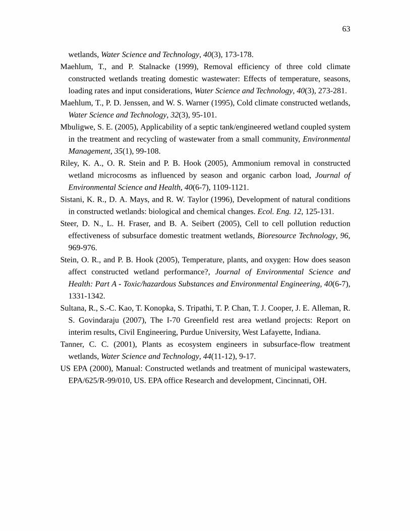
63
wetlands, Water Science and Technology, 40(3), 173-178. Maehlum, T., and P. Stalnacke (1999), Removal efficiency of three cold climate
constructed wetlands treating domestic wastewater: Effects of temperature, seasons, loading rates and input considerations, Water Science and Technology, 40(3), 273-281.
Maehlum, T., P. D. Jenssen, and W. S. Warner (1995), Cold climate constructed wetlands, Water Science and Technology, 32(3), 95-101.
Mbuligwe, S. E. (2005), Applicability of a septic tank/engineered wetland coupled system in the treatment and recycling of wastewater from a small community, Environmental Management, 35(1), 99-108.
Riley, K. A., O. R. Stein and P. B. Hook (2005), Ammonium removal in constructed wetland microcosms as influenced by season and organic carbon load, Journal of Environmental Science and Health, 40(6-7), 1109-1121.
Sistani, K. R., D. A. Mays, and R. W. Taylor (1996), Development of natural conditions in constructed wetlands: biological and chemical changes. Ecol. Eng. 12, 125-131.
Steer, D. N., L. H. Fraser, and B. A. Seibert (2005), Cell to cell pollution reduction effectiveness of subsurface domestic treatment wetlands, Bioresource Technology, 96, 969-976.
Stein, O. R., and P. B. Hook (2005), Temperature, plants, and oxygen: How does season affect constructed wetland performance?, Journal of Environmental Science and Health: Part A - Toxic/hazardous Substances and Environmental Engineering, 40(6-7), 1331-1342.
Sultana, R., S.-C. Kao, T. Konopka, S. Tripathi, T. P. Chan, T. J. Cooper, J. E. Alleman, R. S. Govindaraju (2007), The I-70 Greenfield rest area wetland projects: Report on interim results, Civil Engineering, Purdue University, West Lafayette, Indiana.
Tanner, C. C. (2001), Plants as ecosystem engineers in subsurface-flow treatment wetlands, Water Science and Technology, 44(11-12), 9-17.
US EPA (2000), Manual: Constructed wetlands and treatment of municipal wastewaters, EPA/625/R-99/010, US. EPA office Research and development, Cincinnati, OH.
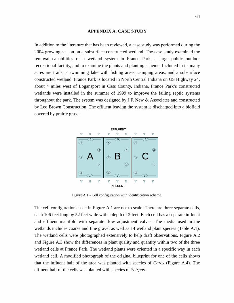
64
APPENDIX A. CASE STUDY In addition to the literature that has been reviewed, a case study was performed during the 2004 growing season on a subsurface constructed wetland. The case study examined the removal capabilities of a wetland system in France Park, a large public outdoor recreational facility, and to examine the plants and planting scheme. Included in its many acres are trails, a swimming lake with fishing areas, camping areas, and a subsurface constructed wetland. France Park is located in North Central Indiana on US Highway 24, about 4 miles west of Logansport in Cass County, Indiana. France Park’s constructed wetlands were installed in the summer of 1999 to improve the failing septic systems throughout the park. The system was designed by J.F. New & Associates and constructed by Leo Brown Construction. The effluent leaving the system is discharged into a biofield covered by prairie grass.
12
3
4
6
7
5
12
3
4
6
7
5
12
3
4
6
7
5
A B C
EFFLUENT
INFLUENT
Figure A.1 - Cell configuration with identification scheme. The cell configurations seen in Figure A.1 are not to scale. There are three separate cells, each 106 feet long by 52 feet wide with a depth of 2 feet. Each cell has a separate influent and effluent manifold with separate flow adjustment valves. The media used in the wetlands includes coarse and fine gravel as well as 14 wetland plant species (Table A.1). The wetland cells were photographed extensively to help draft observations. Figure A.2 and Figure A.3 show the differences in plant quality and quantity within two of the three wetland cells at France Park. The wetland plants were oriented in a specific way in each wetland cell. A modified photograph of the original blueprint for one of the cells shows that the influent half of the area was planted with species of Carex (Figure A.4). The effluent half of the cells was planted with species of Scirpus.
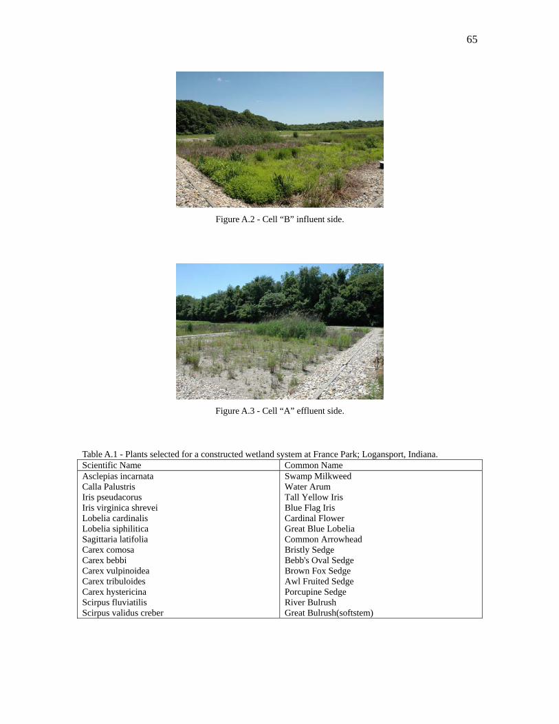
65
Figure A.2 - Cell “B” influent side.
Figure A.3 - Cell “A” effluent side.
Table A.1 - Plants selected for a constructed wetland system at France Park; Logansport, Indiana. Scientific Name Common Name Asclepias incarnata Calla Palustris Iris pseudacorus Iris virginica shrevei Lobelia cardinalis Lobelia siphilitica Sagittaria latifolia Carex comosa Carex bebbi Carex vulpinoidea Carex tribuloides Carex hystericina Scirpus fluviatilis Scirpus validus creber
Swamp Milkweed Water Arum Tall Yellow Iris Blue Flag Iris Cardinal Flower Great Blue Lobelia Common Arrowhead Bristly Sedge Bebb's Oval Sedge Brown Fox Sedge Awl Fruited Sedge Porcupine Sedge River Bulrush Great Bulrush(softstem)
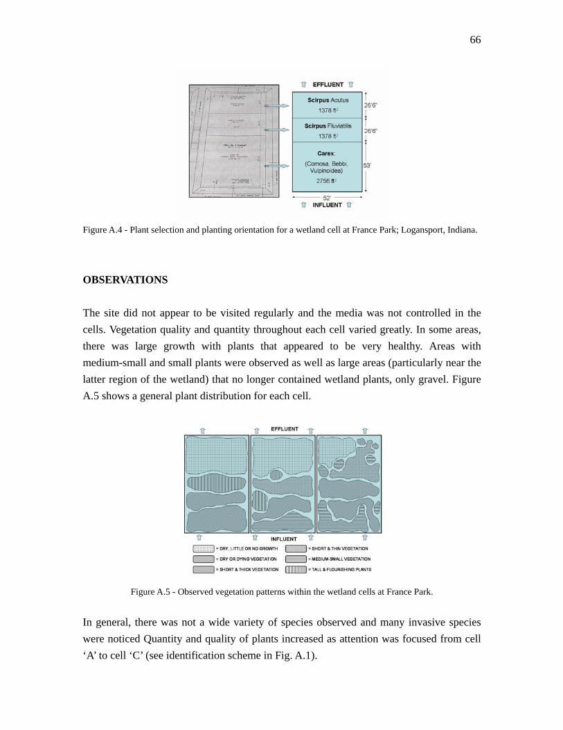
66
Figure A.4 - Plant selection and planting orientation for a wetland cell at France Park; Logansport, Indiana.
OBSERVATIONS The site did not appear to be visited regularly and the media was not controlled in the cells. Vegetation quality and quantity throughout each cell varied greatly. In some areas, there was large growth with plants that appeared to be very healthy. Areas with medium-small and small plants were observed as well as large areas (particularly near the latter region of the wetland) that no longer contained wetland plants, only gravel. Figure A.5 shows a general plant distribution for each cell.
Figure A.5 - Observed vegetation patterns within the wetland cells at France Park.
In general, there was not a wide variety of species observed and many invasive species were noticed Quantity and quality of plants increased as attention was focused from cell ‘A’ to cell ‘C’ (see identification scheme in Fig. A.1).
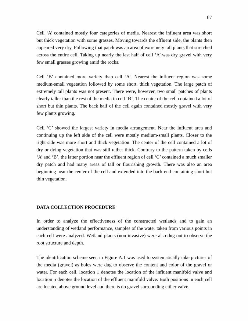
67
Cell ‘A’ contained mostly four categories of media. Nearest the influent area was short but thick vegetation with some grasses. Moving towards the effluent side, the plants then appeared very dry. Following that patch was an area of extremely tall plants that stretched across the entire cell. Taking up nearly the last half of cell ‘A’ was dry gravel with very few small grasses growing amid the rocks. Cell ‘B’ contained more variety than cell ‘A’. Nearest the influent region was some medium-small vegetation followed by some short, thick vegetation. The large patch of extremely tall plants was not present. There were, however, two small patches of plants clearly taller than the rest of the media in cell ‘B’. The center of the cell contained a lot of short but thin plants. The back half of the cell again contained mostly gravel with very few plants growing. Cell ‘C’ showed the largest variety in media arrangement. Near the influent area and continuing up the left side of the cell were mostly medium-small plants. Closer to the right side was more short and thick vegetation. The center of the cell contained a lot of dry or dying vegetation that was still rather thick. Contrary to the pattern taken by cells ‘A’ and ‘B’, the latter portion near the effluent region of cell ‘C’ contained a much smaller dry patch and had many areas of tall or flourishing growth. There was also an area beginning near the center of the cell and extended into the back end containing short but thin vegetation. DATA COLLECTION PROCEDURE In order to analyze the effectiveness of the constructed wetlands and to gain an understanding of wetland performance, samples of the water taken from various points in each cell were analyzed. Wetland plants (non-invasive) were also dug out to observe the root structure and depth. The identification scheme seen in Figure A.1 was used to systematically take pictures of the media (gravel) as holes were dug to observe the content and color of the gravel or water. For each cell, location 1 denotes the location of the influent manifold valve and location 5 denotes the location of the effluent manifold valve. Both positions in each cell are located above ground level and there is no gravel surrounding either valve.
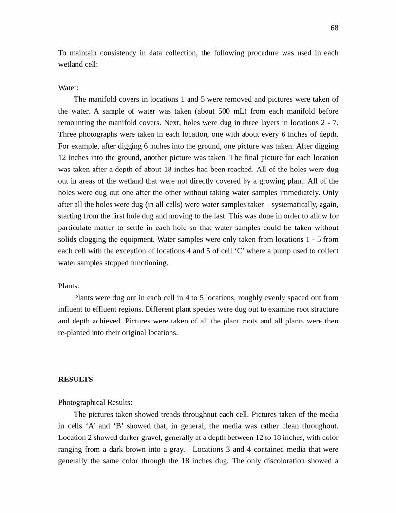
68
To maintain consistency in data collection, the following procedure was used in each wetland cell: Water:
The manifold covers in locations 1 and 5 were removed and pictures were taken of the water. A sample of water was taken (about 500 mL) from each manifold before remounting the manifold covers. Next, holes were dug in three layers in locations 2 - 7. Three photographs were taken in each location, one with about every 6 inches of depth. For example, after digging 6 inches into the ground, one picture was taken. After digging 12 inches into the ground, another picture was taken. The final picture for each location was taken after a depth of about 18 inches had been reached. All of the holes were dug out in areas of the wetland that were not directly covered by a growing plant. All of the holes were dug out one after the other without taking water samples immediately. Only after all the holes were dug (in all cells) were water samples taken - systematically, again, starting from the first hole dug and moving to the last. This was done in order to allow for particulate matter to settle in each hole so that water samples could be taken without solids clogging the equipment. Water samples were only taken from locations 1 - 5 from each cell with the exception of locations 4 and 5 of cell ‘C’ where a pump used to collect water samples stopped functioning. Plants:
Plants were dug out in each cell in 4 to 5 locations, roughly evenly spaced out from influent to effluent regions. Different plant species were dug out to examine root structure and depth achieved. Pictures were taken of all the plant roots and all plants were then re-planted into their original locations. RESULTS Photographical Results:
The pictures taken showed trends throughout each cell. Pictures taken of the media in cells ‘A’ and ‘B’ showed that, in general, the media was rather clean throughout. Location 2 showed darker gravel, generally at a depth between 12 to 18 inches, with color ranging from a dark brown into a gray. Locations 3 and 4 contained media that were generally the same color through the 18 inches dug. The only discoloration showed a
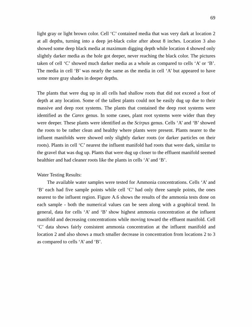
69
light gray or light brown color. Cell ‘C’ contained media that was very dark at location 2 at all depths, turning into a deep jet-black color after about 8 inches. Location 3 also showed some deep black media at maximum digging depth while location 4 showed only slightly darker media as the hole got deeper, never reaching the black color. The pictures taken of cell ‘C’ showed much darker media as a whole as compared to cells ‘A’ or ‘B’. The media in cell ‘B’ was nearly the same as the media in cell ‘A’ but appeared to have some more gray shades in deeper depths.
The plants that were dug up in all cells had shallow roots that did not exceed a foot of depth at any location. Some of the tallest plants could not be easily dug up due to their massive and deep root systems. The plants that contained the deep root systems were identified as the Carex genus. In some cases, plant root systems were wider than they were deeper. These plants were identified as the Scirpus genus. Cells ‘A’ and ‘B’ showed the roots to be rather clean and healthy where plants were present. Plants nearer to the influent manifolds were showed only slightly darker roots (or darker particles on their roots). Plants in cell ‘C’ nearest the influent manifold had roots that were dark, similar to the gravel that was dug up. Plants that were dug up closer to the effluent manifold seemed healthier and had cleaner roots like the plants in cells ‘A’ and ‘B’. Water Testing Results:
The available water samples were tested for Ammonia concentrations. Cells ‘A’ and ‘B’ each had five sample points while cell ‘C’ had only three sample points, the ones nearest to the influent region. Figure A.6 shows the results of the ammonia tests done on each sample - both the numerical values can be seen along with a graphical trend. In general, data for cells ‘A’ and ‘B’ show highest ammonia concentration at the influent manifold and decreasing concentrations while moving toward the effluent manifold. Cell ‘C’ data shows fairly consistent ammonia concentration at the influent manifold and location 2 and also shows a much smaller decrease in concentration from locations 2 to 3 as compared to cells ‘A’ and ‘B’.

70
Ammonia Concentration vs. Location
0
10
20
30
40
50
60
0 1 2 3 4 5
Location (Inlet towards Outlet)
NH
3-N
(mg/
L)
6
Cell "A" Cell "B" Cell "C" Figure A.6 - Ammonia concentrations vs. locations within cells A-C.
DATA ANALYSIS Taking into account the visual observations of the media growth within each cell (Fig. A.2 & A.3), the photographs taken of the vegetation and media, and the results of the tests performed on the water samples, several conclusions can be reached regarding the wetland system at France Park. The photographs taken of the plants as well as the observations seen in Fig. A.5 show many more plants growing in cell ‘C’ as compared to cells ‘A’ and ‘B’ as well as larger root systems for the plants in cells ‘B’ and ‘C’. There is a greater breadth of species in cell ‘C’ as well. There is much less dry area nearest the effluent region of cell ‘C’ as compared to cells ‘A’ and ‘B’. Pictures taken of the gravel show the media to be darker in cell ‘C’ than that of cells ‘A’ or ‘B’. This dark color of the gravel and roots shows that not as much oxygen as reached at those particular locations resulting in ferrous ions to accumulate, resulting in the dark colors. Furthermore, the pictures of the water near the valves at locations 1 and 5 of cell ‘C’ show water that is much dirtier (darker) when compared to same locations of cells ‘A’ or ‘B’. Cell ‘B’, however, has dirtier water at locations 1 and 5 as compared to cell ‘A’. The water at locations 1 and 2 of cell ‘C’ smelled considerably worse than the same locations of cells ‘A’ or ‘B’.
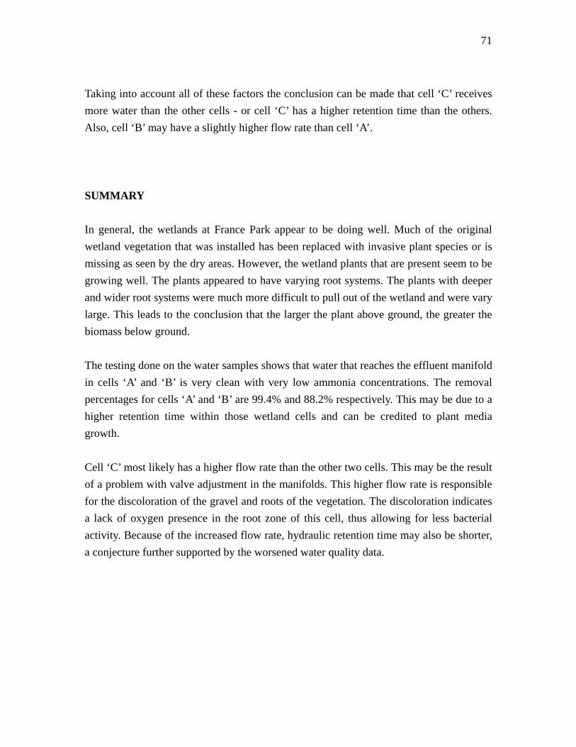
71
Taking into account all of these factors the conclusion can be made that cell ‘C’ receives more water than the other cells - or cell ‘C’ has a higher retention time than the others. Also, cell ‘B’ may have a slightly higher flow rate than cell ‘A’. SUMMARY In general, the wetlands at France Park appear to be doing well. Much of the original wetland vegetation that was installed has been replaced with invasive plant species or is missing as seen by the dry areas. However, the wetland plants that are present seem to be growing well. The plants appeared to have varying root systems. The plants with deeper and wider root systems were much more difficult to pull out of the wetland and were vary large. This leads to the conclusion that the larger the plant above ground, the greater the biomass below ground. The testing done on the water samples shows that water that reaches the effluent manifold in cells ‘A’ and ‘B’ is very clean with very low ammonia concentrations. The removal percentages for cells ‘A’ and ‘B’ are 99.4% and 88.2% respectively. This may be due to a higher retention time within those wetland cells and can be credited to plant media growth. Cell ‘C’ most likely has a higher flow rate than the other two cells. This may be the result of a problem with valve adjustment in the manifolds. This higher flow rate is responsible for the discoloration of the gravel and roots of the vegetation. The discoloration indicates a lack of oxygen presence in the root zone of this cell, thus allowing for less bacterial activity. Because of the increased flow rate, hydraulic retention time may also be shorter, a conjecture further supported by the worsened water quality data.

72
APPENDIX B. WETLAND PROJECT TIMELINE Time Items Remarks June, 2000 Original JTRP proposals (Purdue)
The original research project was developed in a set of 3 proposals submitted to Joint Transportation Research Program (JTRP):
• Constructed Wetlands for INDOT Rest Stop Wastewater Treatment: Proof-of-Concept Research Investigation
• Constructed Wetland Systems for Wastewater Management
• Hydrology of Natural and Constructed Wetlands Biofield Cost Estimated by JF New -- $29,600
June, 2000 Feasibility study (JF New) Key points in the document:
• Proposed a horizontal plug-flow constructed wetland pretreatment system
• Average daily flow: 5,000 gpd; Peak daily flow: 15,000 gpd
• 11,000 ft² surface area • Acknowledged poor nitrogen removal efficiency
(17%) in winter months • Cost estimates: one 10,000 septic tank + 11,000 ft²
wetland cell $133,800
• Annual O/M cost: $1,200
Assuming a cell depth of 1.5 ft, HRT for the wetland is 3.4 days for peak flow and 7.4 days for average flow. Adding a 10,000-gal septic tank will increase the HRT by 0.7 day for peak flow and 2 days for average flow.
Aug, 2000 Combined proposal (Purdue) The 3 original proposals were consolidated into one master “INDOT Rest Stop Constructed Wetland Evaluation” project with 3 components:
• Biofield Unit Placement • Hydraulic Aspects • Environmental Aspects
However, for accounting purposes the three projects were still kept separately.
Aug, 2000 Evaluation of treatment options (Email from Mark L. Sneathen, RQAW, Aug. 14) Presented 3 options:
• Option 1: Paying surcharge and installing ozonatoro Cap. cost: $30,000 o Annual O/M: $3,000
• Option 2A: Wetland pretreatment with no biofield o Cap. cost: $222,000 o Annual O/M: $1,875
• Option 2B: Wetland with biofield o Cap. cost: $222,000 + $35,000 o Annual O/M: $510
• Option 3: Biomechanical pretreatment system o Cap. cost: > $270,000 o Annual O/M: $20,000
For Option 2B, it was assumed that all the effluent was discharged to the biofield.
Oct, 2000 SAC meeting (Oct. 23) • Purdue would pay for construction of the biofield • Estimated construction time: Spring 2001 • Barry Partridge would like to see the following
items discussed in the final report: o Cost comparisons
73
o Performance of wetland and biofield o Wetland vegetation o O/M of wetland system o Design guidelines
Nov, 2000 Batch system design (JF New) JF New proposed a design with an alternating drain-and-fill cycle between the two parallel wetland cells.
Feb, 2001 SAC meeting (Feb. 27) • Due to high ammonia loads, lime stone was
suggested to mix in with the gravel for the wetland medium to increase buffer capacity (alkalinity).
• Proposed instrumentation for the system was presented by Tom Cooper.
• Effluent filters were suggested for the septic tank. • Tentative construction schedule was discussed.
Construction permit had not been obtained. Expected completion date: July 4.
Apr, 2001 Construction cost estimate proposal (Apr. 26) (RQAW, Berns Construction Company, Heritage Industrial Servies) Entire construction cost was estimated to be: $418,975
May, 2001 Retrospective cost analysis (RQAW, JF New, Purdue) Comments from JF New:
• Drew Bender o Public job more expensive o Higher ammonia loading o Larger biofield (poor soil loading rate) o “Bell and whistles”
• Ted Blahnik o Design flow increase: 5,000 gpd 10,000 gpdo Additional effluent piping o Recirculation system o Aeration chamber o Sampling and monitoring equipement
Comments from RQAW (Mark Sneathen): • Essentially same design flow (smaller wetland
surface area) • One extra septic tank • Force main from softener building
Analysis by Purdue: • Reduced surface area but increase in depth (1.5 ft
2.75 ft) • Change of system operating mode: from
conventional plug-flow to batch cyclic drain-and-fill
• Apparent increase in cost due to non-competitive bidding
June, 2001 Strategic plan (Purdue, Jun. 7) A game plan was prepared to outline the steps leading to the construction of the wetland system.
July, 2001 Revised Design (Jul. 2, Purdue) In an effort to reduce construction cost and streamline treatment design, Purdue proposed a revised wetland system with the following items:
• Additional third wetland cell for effluent polishing

74
• A much smaller biofield • Recirculation to the second septic tank
Purdue would pay for the re-design costs of the system. Oct, 2001 SAC meeting (Oct. 11)
• Gary Duncan (RQAW) presented the revised wetland design.
Oct, 2002 SAC Meeting (Oct. 28) • Phase I monies ($100,000) to be used by December,
2002. Request for Phase II monies ($80,000) to be made to the JTRP board in November, 2002.
• Jim Alleman (Purdue) had a discussion with Ed Miller (ISDH) regarding a construction permit for the wetland system. This permit was still not attained.
Tentative meeting scheduled to resolve permitting issues, Nov. 6th.
Dec, 2002 Construction Begins June, 2003 Site Visit & Meeting (Jun. 5)
• Vanderpool and Mason (INDOT) were very concerned with overflow to cells and mentioned alarms needed.
• Neither septic tank had any level sensor or alarm • The access hatch for the flume box was not
gasketed, likely odor. • The issue of shallow side walls and rough
installation of wetland cells brought up the concern for membrane tears or punctures.
JF New was not concerned, claimed 3:1 slope was intended and appropriate.
Aug, 2003 Wetland Cells Planted (Aug. 12) • 3,820 plants, 13 different species.
Oct, 2003 SAC Meeting (Oct. 14) • Implementation time of SCADA system is still
unknown. • Clyde Mason (INDOT) suggested subsurface
discharge • Operation and Maintenance Manual was
discussed. o Responsibilities of Purdue, RQAW and
INDOT to be clearly spelled out. o Tom Vanderpool (INDOT) suggested
“decision tree” structure including emergency procedures and contacts.
• High flow rates from south side ostensible on October 11th caused surges in the first septic tank, preventing settling and submerging the V-notch weir in between septic tank 1 and 2. Discussion of clogged filters and wetland media led to immediate actions.
o South side flow was shut down, leaving only north side flow into the wetland system.
o A meeting with RQAW was requested to determine pump operation data from the south side.
• Installation of a surge tank upstream of septic tanks was discussed.
• Posters of the site were presented. Purdue agreed to
Tight clays make subsurface discharge very difficult.

75
send electronic versions and hard copies to INDOT, Greenfield.
Oct, 2003 Pre-Startup Meeting (Oct. 27) • The need for an emergency generator was
discussed. o Clyde Mason (INDOT) said power was
lost to the site often. o A high demand on the electric system
could cause problems including heat buildup in system panels.
• Flow sheets reviewed for September, 2003 showed 9k-10k maximum per-day average for the system.
• High pumping rate from south side. Discussed solutions included installing a smaller diameter force main, constructing a surge tank, or (ideally) putting a septic tank on the south side.
• Flow from the pumps (LS1) should have been around 72 GPM, but were measured at 38 GPM - it was determined that some kind of restriction was the problem, possibly a check valve problem.
• Heritage to sort out problems with pumps and outlets. Purdue to start looking at settleability from water samples. JF New to develop O & M draft. RQAW to develop surge tank design and cost estimate.
Existing demand is 44.5 kW, 2/3 of service (66 kW). Proposed generator to use natural gas to drop demand.• 100 kW generator
costs $20k-$24k • 200 amp breaker to
reduce load by ½ costs $40k-$65k
Nov, 2003 Pre-Startup Video Conference (Nov. 6) • The 38 GPM pumping rate from LS1 was still a
problem; a pipe was supposedly crushed. Brian Morgan was to fix the problem.
• Postponement of surge tank design was decided until LS1 becomes fully functional so that the surging problem can be re-examined.
• Discussion of the V-notch weir led to the conclusion that the septic tanks should be checked by a certified inspector.
• The O & M manual was to be completed by JF New by Nov. 25th.
Dec, 2003 (Dec. 22) Wastewater samples collected by Purdue for analysis.
Dec, 2003 30,000 GPD flow rate recorded (Dec. 29) System was temporarily shut down. Westbound wastewater was now fed into the wetland system while eastbound wastewater was sent back to the city. Recirculation was terminated.
Normal flow rate should be 5,000 GPD.
Mar, 2004 On-Site Meeting (Mar. 5) • Gary Duncan (RQAW) pointed out insufficient gas
line and suggested installation of new regulator, $25,000 cost.
• Decision reached to proceed with surge tank design (RQAW, JF New) based on estimated 400 GPM flow from south side.
• SCADA system cost estimate was to be determined by Gary Duncan. A meeting was suggested for further discussion.
• Magmeter M2 was not working (bad coil on the
76
sensor) and was given to Tom Cooper for repair. • Installation of a concrete base for the weather
station was to be provided by Bryan Morgan according to Tom Cooper’s spec’s.
Mar, 2004 SAC Meeting (Mar. 19) • T. P. Chan (Purdue) provided an update of activities
and problems that were encountered. Spikes in the flow data were discussed.
• The septic tanks had been pumped and cleaned. Sludge was about 2 ft. from the top. Costs were $530 per 400 gallons.
• Surge tank design had started (Gary Duncan). Clyde Mason (INDOT) suggested that any flow over 10,000 GPD be diverted to the city without flow through wetlands.
• Barry Partridge (INDOT) wanted to see the following in a report:
o Economics of having a wetland-biofield with and without access to city POTW.
o Impact of winter months. o Site properties conducive for this
technology.
May, 2004 SAC Meeting (May 25) • Voltage surges resulted in complete system
shutdown during the last week of March. • SCADA System - T. P. Chan (Purdue) suggested
that a 3-way valve is installed to control drainage to maximize system HRT.
• New generator designs will be sent to INDOT by RQAW.
• Discussion of a tentative surge tank design included:
o A 5,000 gallon tank, at least 5’ of free board.
o (2) 72 GPM grinder pumps (time controlled).
o Three floats - High, Low, Low-Low. o Located next to North side lift station. o Magmeter installed to monitor total
feeding flow. • Cell 3 plants were not doing well. Dave (JF New)
said there is a maintenance issue resulting in no warranty.
• Many invasive plants were found in the cells and wetland plant roots did not extend past the peat layer. Dave (JF New) suggested that water levels be lowered, said there was lack of nutrients.
• High groundwater table caused water pockets to form under cell liners. Flow data could have been affected by leaks in the system.
• F-3 Ultrasound sensor was damaged due to high water levels.
• Brian Morgan (Heritage) fixed the check valve problem; LS-4 functions at full capacity now.
• Gary Duncan resigned, Matt Moore new RQAW
Elec. Company lowered voltage to “fix” problem. Voltage problems caused flooding. If 30% or more plants die within 1 yr. of planting, more would be considered.
77
project manager. June, 2004 Purdue University (Jun. 7)
A new data logger was installed by Tom Cooper in order to store more data. Data will not need to be collected as often.
Tank is only 4,000 gallons.
June, 2004 SAC Meeting (Jun. 15) • A gas generator will be set up with a 200 amp
capacity. • David Latka (JF New) presented the final design of
the surge tank. • Greg Pankow (INDOT) stated that INDOT wants to
wrap up their contractual bindings. • An agreement was reached to follow through with
the surge tank. JF New was to deliver plans to RQAW by the end of June, RQAW to deliver to Heritage by 1st week of July, Heritage will send price to INDOT by the 2nd week of July.
• SCADA plans were ready and were to be delivered by John Downs (Integrity) will deliver them to Heritage through RQAW.
Sept, 2004 SAC Meeting (Sept. 23) • Performance of the wetland was noted to be less
than desired. • Monies allocated in 2000 are still being used by
Purdue, and would likely last another year before additional funds would be requested.
• A new cost estimate for the surge tank was less than originally anticipated (note that the size has changed to 4,000 gallon cap.).
• INDOT (Greg Pankow and others) expressed their desire to have all construction at the site be completed by the end of this calendar year (December 2004).
• The issue of weeds was brought up by Jim Alleman.Jim said that he would contact JF New regarding maintenance of the wetland.
June, 2005 System instrumentation damaged, presumably by lightening
• Five pieces of equipment were damaged. Tom Cooper sent these instruments back to dealers for repair.
Unable to monitor flow at all stations due to broken equipment.
June, 2005 Surge Tank Installation Began • 4,000 gallon surge tank • North side of the rest area (west bound lanes)
installed near the restroom building.
Aug, 2005 SAC Meeting (Aug. 26) • Invasive species were becoming a problem.
Responsibility of removal was uncertain and expertise was limited. Clyde Mason said that he would find out if one of the herbicide coordinators could be trained to take care of this.
• A power surge (presumably from a lightening strike) damaged some instrumentation in June of 2005.
o 5 instruments had been damaged and sent
Purdue created electronic file of wetland plant information for original species planted.

78
back to dealers for repair. o The instruments have since arrived and
will be reinstalled. • Tom Duncan said he would find out more about the
status of the SCADA system over the next week. • INDOT (Greg Pankow) expressed concern that
there had been no representative from FHWA in the past several meetings.
• Effluent quality was reported by Purdue: o High percentage removal in wetland cells.o Surface discharge standards are not yet
met, but the water may qualify for discharge to the city without surcharges.
• Biofield sampling is to be conducted in the future.• INDOT (Greg Pankow) stated that the project needs
to be closed soon. SCADA and generator still have not been paid for.
• Steve Land informed the group that there was a possibility of the first septic tank might have developed a crack; it may need repair.
Aug, 2005 Surge Tank Installation Completed • Presumably, flow restored to wetland through the
storage tank.
Feb, 2006 SAC Meeting (Feb. 24) • Presumably, the current state of the wetland was
discussed. o The wetland plant species in all cells were
affected by the surge tank installation where flow was restricted to the wetland system.
o Many plant species are no longer present, and the remaining plants appear to be dying.
o A vast amount of invasive species (weeds) are present in the cells.
• Presumably, JF New will decide whether or not to replant the wetland cells based on the wetland species’ ability to re-grow.
May, 2006 Wetland Cells replanted • Clyde Mason replanted all of the wetland cells with
a number of plants. After observation it was noted that not all original plant species were replanted, only a select few.
June, 2006 SAC Meeting (Jun. 7) • Presumably, water effluent quality was discussed. • A downward trend was noted in effluent quality.
TSS, NH3, and BOD removal have been decreased, possibly due to inconsistent flow to the wetlands, which may have caused the plants to die and decrease in quantity, thus causing the decreased removal.
o A possible need to replant the wetland cells may be justified.
• Presumably, water flow data was discussed. o There are gaps in the flow data.

79
• Equipment failure after the presumed lightening strike.
• The data logger was unplugged during surge tank construction and SCADA system installation.
• There are inherent measurement problems with the instruments.
o Rebeka Sultana has developed a hydraulic model of the wetland system.
• The SCADA system was discussed. o Data since January 2006 was in question
as to who had it and how it could be accessed.
o A training schedule for the SCADA system is needed.
o Web access of the system and/or data - is this possible?
• Recycle pumps are not working as of May 22, 2006.
• Data from the biofield was discussed. o Samples are only available from the
deepest well. o Samples show that treatment is not as
desired and flow to the biofield should be shut off.
• Data availability was discussed. Should raw data be put on a website or is data presented at meetings enough detail?
April, 2007 SAC Meeting (Apr. 24) • Problems with the SCADA system were identified
and discussed. o Clyde Mason mentioned that flow rates
outputted by the system were high; beyond 5000 gpd as expected.
o SCADA data was not available through the system’s website for a number of weeks.
o Joan Wooldridge stated that controlling flow rates into the wetland system from the surge tank is difficult.
o Clyde Mason stated that Integrity Systems had asked for more funds to fix the SCADA system.
• New shredder pumps were installed in the surge tank in late January, 2007.
• Wetland cost information was requested of INDOT by Purdue University in order to perform a cost study of the Greenfield wetland.
• INDOT determined that the septic tanks need to be emptied at least once a month to prevent clogging.
• Clyde Mason informed of the use of high pressure emitters to release the wetland effluent into the landscape in a controlled manner.