The hydrodynamics equations allow for the formation of

arbitrarily large and arbitrarily localized

spatial variations

of the hydrodynamical variables,

which are mathematically treated as discontinuities and are often referred to as shocks.

(inviscid) Burger’s equation

!

"u"t

+ u"u"x

= 0

In general, difficulties arise when a Cauchy problem described by a set of continuous PDEs is solved in a discretised form: the numerical solution is, at best, piecewise constant.

The nonlinear properties of the hydrodynamical equations for compressible fluids generically produce, in a finite time, nonlinear waves with discontinuities (i.e. shocks) even from smooth initial data.

Since the occurrence of discontinuities is a fundamental property of the hydrodynamical equations, any numerical scheme must be able to handle them in a satisfactory way.

Possible solutions to the discontinuity problem:

!  1st order accurate schemes "  generally fine, but very inaccurate across discontinuities (excessive

diffusion); e.g. Lax-Friedrichs method

!

u in +1 =

12

(u i+1n + u i-1

n ) " #t2#x

Fi+1 " Fi"1( )

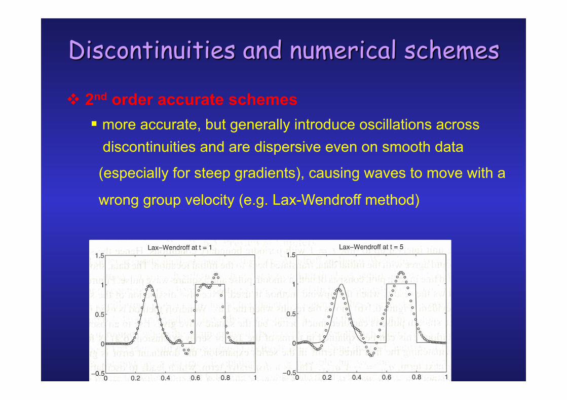
!  2nd order accurate schemes "  more accurate, but generally introduce oscillations across discontinuities and are dispersive even on smooth data

(especially for steep gradients), causing waves to move with a

wrong group velocity (e.g. Lax-Wendroff method)

! 2nd order accurate schemes with artificial viscosity "  mimic Nature, but problem-dependent and inaccurate for

ultrarelativistic flows

!  Godunov methods "  discontinuities are not eliminated, rather they are exploited "  based on the solution of Riemann problems "  ~second-order schemes can be derived "  state of the art in relativistic hydrodynamics

Riemann problem

Definition: in general, for a hyperbolic system of equations, a Riemann problem is an initial-value problem with initial condition given by:

where UL and UR are two constant vectors representing the left and right state.

For hydrodynamics, a (physical) Riemann problem is the evolution of a fluid initially composed of two states with different and constant values of velocity, pressure and density.

Riemann problem

!!"# !!"$ ! !"$ !"#

%&'()*'&+,(&-

!

!"$

!"#

!".

/0&12)3,-42',(

*/(3'256$!

78/3348/6$!

9/-,1'25

Riemann problem

rarefaction

contact discontinuity

shock

density

pressure

velocity

Godunov’s idea Core idea: a piecewise-constant description of hydrodynamical quantities will produce a collection of local Riemann problems, whose solution can be found exactly (if one wishes).

This is an example of how research in basic physics can boost computational methods.

“Riemann problems”

In HRSC methods, higher order of accuracy is reached with a better representation of the solution: that is with a ”reconstruction” of the solution.

Such a reconstruction can be made with different algorithms.

The values of the reconstructed function on the cell boundaries are then used as the initial data for the Riemann problems at the cell boundaries.

A useful measure of the oscillations present in the numerical solution is provided by the notion of total variation:

!

TV(Q) " |Qi #i=#$

$

% Qi#1 |

For this to be a meaningful measure, Q must become constant at infinity. Usually Q has compact support, anyway.

A sufficient condition that ensures that a method does not introduce oscillations is that its total variation does not increase:

Standard TVD reconstruction methods consist in approximating the solution with a piecewise linear function.

Different TVD reconstruction methods differ in the way in which the slope (linear approximation) is selected. The selected slope is a combination of the upwind Sup, downwind Sdown and central Sc slopes.

!

Sup =xi " xi"1#x

Sdown =xi+1 " xi#x

Sc =xi+1 " xi"12#x

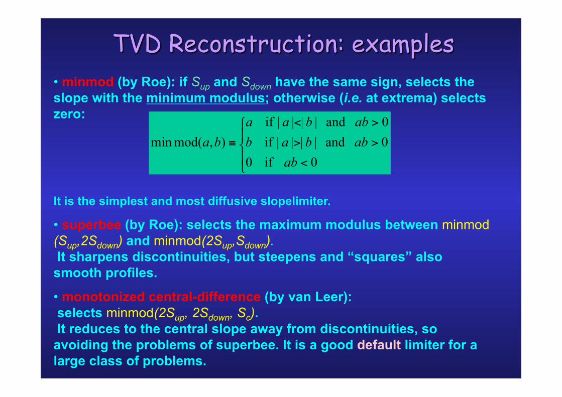
•  minmod (by Roe): if Sup and Sdown have the same sign, selects the slope with the minimum modulus; otherwise (i.e. at extrema) selects zero:

It is the simplest and most diffusive slopelimiter.

•  superbee (by Roe): selects the maximum modulus between minmod(Sup,2Sdown) and minmod(2Sup,Sdown). It sharpens discontinuities, but steepens and “squares” also smooth profiles.

•  monotonized central-difference (by van Leer): selects minmod(2Sup, 2Sdown, Sc). It reduces to the central slope away from discontinuities, so avoiding the problems of superbee. It is a good default limiter for a large class of problems.

As said earlier, ENO methods are not TVD, but

!

TV(Qn+1) " TV(Qn ) +O(#xk+1) their total variation is bound to grow only slowly.

ENO methods are more expensive than TVD ones and, in my experience, it is not worth to go to higher than 4th order, in which case, anyway, their accuracy is not better than PPM (see later slides), for example.

There are numerous variants of ENO methods. The basic idea is to choose a stencil including s+t<k+1 cells (s to he left of the point and t to its right), so that the smoothest reconstruction is achieved.

cfr. e.g.: Shu C.W., in T.J. Barth, H. Deconinck (eds.), High-Order Methods for Computational Physics, Springer (1999).

The smoothness is measured in terms of the Newton divided differences:

!

n[xi"1,xi] #ui " ui"1xi " xi"1

After the stencil giving the minimum Newton divided differences is found, a k-order polynomial interpolation gives the reconstructed value on the i-th cell interface.

The property:

illustrates how minimising the Newton divided differences provides the smoothest reconstruction. !

n[xi"s,xi+ t ] =n(t+s)(#)(t + s)!

where n(t+s) is the (t+s)-th derivative

Piecewise Parabolic Method (PPM)

•  PPM is a rather more complex, composite procedure to achieve, theoretically, third order accuracy.

•  In practice it is not much above second order, but it is more accurate.

•  It has several (7 in our implementation) adjustable parameters; which add to its complexity

•  In Whisky only part of the method is implemented and specialised it to an evenly spaced grid.

•  PPM requires a stencil of three or four points (depending on which parts of the scheme are used).

•  The basic idea is to construct in each cell an interpolating parabola, such that its integral average coincides with the known solution and that no new extrema appear in the interpolated function.

Colella, Woodward, J. Comput. Phys, 54, 174 (1984)

Summary of reconstruction methods •  Reconstruction methods serve the purpose of increasing the order of accuracy of the scheme

•  They reconstruct the data on the cell boundaries, starting from the data at the cell centres

•  They set the initial conditions for the local Riemann problems

•  Different type of reconstruction methods are available: TVD, ENO, …

•  Some famous examples:

•  slope limiters: linear but reduce the order to 1 at extrema:

•  minmod: the most diffusive

•  superbee: squares waves

•  MC: combines the good properties of the above two methods

•  ENO: any order (in theory)

•  PPM: expensive, but accurate

•  In principle one could solve “exactly” the Riemann problem at each cell interface.

•  “Exactly” does not mean analytically, but via the numerical solution of a non-linear algebraic equation. As far as the solution of partial differential equations is concerned, this is “exact” .

•  However, exact solvers are computationally too expensive, so “approximate” Riemann solvers [Roe, Marquina, HLL(E,C,...), etc.] are instead used in place of the exact ones.

•  In the following I will present some popular approximate Riemann solvers.

Summary about Riemann solvers

•  Riemann solvers are essential to building numerical methods that well describe discontinuities

•  exact Riemann solvers are computationally (prohibitively) costly •  several approximate Riemann solvers have been proposed, e.g.

•  HLLE: simple, robust, computationally relatively inexpensive, rather dissipative

•  Roe: more computationally expensive, less dissipative; problems at sonic points

•  Marquina: like Roe, with improvement at sonic points

Going from 1D to 3D The easiest way of extending 1D schemes to 3D is dimensional splitting,

i.e. obtaining the 3D procedure as a sequence of three 1D operations. It is easy to implement, computationally convenient and the error is usually smaller then the error of the individual 1D schemes.

The solution of the 3-dimensional equation

can be approximated by the solution of a sequence of 1D equations as follows:

The order of the operations does not affect the accuracy of the schemes.

!

"tU +# $ F(U) = 0U(! x ,t n ) = U n

% & '

!

"tU* + "

x1F(U*) = 0

U*(! x ,t n ) = U n

# $ %

& %

!

"tU** + "

x 2F(U**) = 0

U**(! x ,t n ) = U*

# $ %

& %

!

"tU + "x 3

F(U) = 0

U(! x ,t n ) = U**

# $ %

!

Un+1

References •  R. J. Leveque, Finite Volume Methods for Hyperbolic

Problems, Cambridge University Press

•  E. F. Toro, Riemann Solvers and Numerical Methods for Fluid Dynamics, Springer

•  Leveque R.J., Numerical Methods for Conservation Laws, Birkhauser Verlag

Summary of the first lecture •  definition of fluid and shock •  finite-volume methods for conservative systems: evolve the

integral average on a numerical cell by means of the fluxes between adjacent cells

•  weak solutions •  theorems on conservative numerical methods •  Riemann problem: three kinds of waves •  Godunov’s idea •  Godunov’s algorithm •  Rankine-Hugoniot condition