the gwx story - inforuminforumweb.umd.edu/papers/conferences/2017/usa_almon_2017.pdf · i soon...
TRANSCRIPT

The Gwx StoryThe Biography of a Regression and Model-building Program
Built in C++ with Free, Open-Source,Cross-Platform Tools
Clopper Almon
A Partial and Preliminary Version as of
May 2017

This book is published under
the Creative Commons AttributionNon Commercial License.
The details of this license can be seen at
https://creativecommons.org/licenses/bync/4.0/legalcode
May 22, 2017
2

ContentsMotivation..................................................................................................................................................6 Gwx Tutorial 1: The Basic Framework...................................................................................................10
Getting the Tools: C++, wxWidgets and Code::Blocks in Ubuntu Linux...........................................10The Gwx Framework...........................................................................................................................11Backup files.........................................................................................................................................12Restoring printf().................................................................................................................................13Initializing Variables and the Event Table...........................................................................................15Getting Input from the User and Handling the Items List in a Combobox.........................................17
Gwx Tutorial 2: The Select-Chop Interaction..........................................................................................19Customizing the Code::Blocks Screen................................................................................................19Select and Chop...................................................................................................................................19
Gwx Tutorial 3: Drawing and Saving Graphs..........................................................................................24Basic Drawing on the Screen..............................................................................................................24A Stretchable Canvas for Giotto..........................................................................................................27Drawing Straight Lines, an Octagon...................................................................................................28Putting Text on the Graph....................................................................................................................29Saving Graphs as .PNG and .JPG Files...............................................................................................31
Gwx Tutorial 4: The Debugger, an Improved Chop(), and Text Substitution..........................................34The Code::Blocks Debugger with GNU GCC....................................................................................34Refining chop()....................................................................................................................................35Making Text Substitutions...................................................................................................................38
Tutorial 5: Making printg() Global..........................................................................................................40Picking the Starting Directory.............................................................................................................42Saving and Moving the Gwx Program and Project to Other Computers............................................44The Road Ahead..................................................................................................................................45
Tutorial 6: A Data Bank for Gwx.............................................................................................................47Structure of the Standard G Data Bank...............................................................................................47How Many Names Are Possible?........................................................................................................49Dividing Gwx into Modules and Common.h......................................................................................50Creating a Workspace Bank................................................................................................................52The Bank.cpp Module.........................................................................................................................54Adding a Module to a Code::Blocks Project.......................................................................................58Using namespace and Standard max() and min()................................................................................59The type Command.............................................................................................................................61Time to Test.........................................................................................................................................61
Tutorial 7: Taking Commands from a File: the add Command...............................................................63Tutorial 8: Dates in Gwx: the GDate struct..............................................................................................67
Declaration of the GDate struct and Some Changes to common.h.....................................................68Setting tdates with the tdates Command.............................................................................................70The chopdate() Function.....................................................................................................................71Giving Values to a GDate, the set() Functions....................................................................................72The Observation Number Function, ObNo(), of a GDate...................................................................74
3
The type Command with tdates...........................................................................................................76Test It Out!...........................................................................................................................................78
Tutorial 9: The data and matdata Commands..........................................................................................79First Version; Date on Command Line................................................................................................79Second Version: Negatives, Error Messages, Date Placement Options..............................................82The matdata Command – What It Should Do.....................................................................................87Handling Two-Dimensional Arrays.....................................................................................................88Writing matdatacmd().........................................................................................................................90
Tutorial 10: The f Command....................................................................................................................94First Version – Arithmetic Only and No Parentheses..........................................................................94Constants...........................................................................................................................................100Parentheses........................................................................................................................................100The @log() and @exp functions.......................................................................................................101Lagged values of variables................................................................................................................104
Tutorial 11: Linear Regression: the r Command...................................................................................105The rdates Command.........................................................................................................................105Giving the Regression a Title............................................................................................................107What Size Regression?......................................................................................................................108Reading the r Command....................................................................................................................109
Tutorial 12. Graphs................................................................................................................................120Auxiliary Graphing Commands I: gdates..........................................................................................120Auxiliary Graphing Commands II: vrange and legend.....................................................................122The Plan for the Rest of This Tutorial...............................................................................................126 Reading the Data for a Graph...........................................................................................................126The GraphDialog and a Rudimentary Graph....................................................................................130A DesCartes with Labeling of the Vertical and Horizontal Axes......................................................133The gname Command.......................................................................................................................138Saving Graphs...................................................................................................................................139
Tutorial 13. Assigned Data Banks I.......................................................................................................141Assigning and Referencing Banks....................................................................................................141The DataBank Class..........................................................................................................................142Derivation of the GBank Class from the Abstract DataBank Class..................................................144Functions for the GBank Class..........................................................................................................146The bank Command..........................................................................................................................153Extending getseries() to Use the Assigned Banks.............................................................................154Modification of rhs().........................................................................................................................156Test....................................................................................................................................................158Summary...........................................................................................................................................158
Tutorial 14. Saving Results from Regression: The save and catch Commands; gr * and #...................160Saving and Catching title and f Commands......................................................................................162Writing Regresssion Results into the Save File.................................................................................162Writing Regression Results into the Catch File.................................................................................163The gr * Command for Graphing Regresssion Results.....................................................................164The # Comment.................................................................................................................................164
Tutorial 15: Softly Constrained Regression: The con and sma Commands...........................................166Soft Constraints.................................................................................................................................166The con Command............................................................................................................................167
4
Using the Artificial Observations......................................................................................................171The sma command for estimating distributed lags............................................................................172
Tutorial 16. Useful Functions.................................................................................................................177Create Stocks from Flows – @cum()................................................................................................177Frequency conversion by polynomial interpolation..........................................................................179Annual to Quarterly Conversion – @atoq()......................................................................................182Annual to Quarterly Conversion with an Indicator Series – atoqi()..................................................185Monthly to Quarterly Conversion – @mtoq()...................................................................................189
Tutorial 17: The Road Ahead – Vectors and Matrices...........................................................................191What the G-Only Model Will Do......................................................................................................192How To Do Multisectoral Modeling with Just G7............................................................................192So What Needs to be Written?...........................................................................................................202
Tutorial 18. Creating a VAM File..........................................................................................................204VAM Files from the User's Viewpoint..............................................................................................204Two Preliminaries: gstrcpy() and stringer()......................................................................................206The VamFileDesc struct....................................................................................................................207The vamcreate Code..........................................................................................................................209
Tutorial 19: Assigning a VAM File to be Read......................................................................................217The dvam Command.........................................................................................................................219
Tutorial 20. Reading Data into the VAM file; matin()...........................................................................221Tutorial 21: Using wxGrid.....................................................................................................................225
The Barnum code..............................................................................................................................226Preparing the matrix to be shown: showmat():.................................................................................228
Tutorial 22: Displaying a Matrix from a VamFile..................................................................................231
5

MotivationThe G7 modelbuilding program lies at the heart of Inforum work around the world.
Keeping it alive and well is therefore an important task. Currently,it is built using Borland C++ Builder 6, (BB6). Borland disappeared over ten years ago. BB6 did not work well on Windows Vista, works again on Windows 7, 8 and 10, but may – or may not – stop working onfuture versions of Windows. Meanwhile, free, opensource, crossplatform tools have become available. It seemed eminently desirable to use these tools to build a regression and model building program that would have the basic capabilities of G7, be familiar to users of G7, and would work on Windows, Mac, and Linux.
Thus originated the Gwx project. It is currently developed to the point of having the G7 features most used in macro modeling, especially quarterly as well as annual. These include assigning data banks, reading in data, creating new data series by algebraic formulas, logarithm and exponential functions, the @cum function for creating stocks from flows, the @atoq and @atoqi functions for creating quarterly series from annual series, and the @mtoq()function for making a quarterly series from a monthly one. It does ordinary leastsquares regression, regression with “soft” linear constraints on the regression coefficients and “sma” regression to softly impose polynomial constraints on coefficients of a distributed lag. Results are saved in files which can potentially be used to build models or write papers. It draws graphs with carefully labeled axes and a legend, as well as a title and subtitle. Graphs are saved in the industry standard png format.
This list of features seemed sufficient to warrant this report and to announce that the Linux version is available. I have not tried to compile the Build program under Linux nor to actually build and run a model under Linux, but I do not anticipate great problems because no graphical elements are involved – just straight commandline C++. Nor have I yet tried to create a Mac version, in part because I do not have a Mac. I would welcome help here from a Mac owner.
Gwx does not yet have any of the matrix algebra features associated with VAM (vectorandmatrix) files and most useful for building multi sectoral models. That is the next area of work. (Actually, it can already create an empty VAM file, but that is of little value by itself.)
Gwx is, however, no ordinary program. It has a written biography – this book. I resolved that as I wrote the program, I would try to explain as well as possible the code as it moves from a very simple G to a fairly complete one. The idea of writing the biography of a computerprogram may seem a bit bizarre. I know of no other example. There are plenty of books about how to use a finished program, but the story of how a program grew from something very simple to something quite complex seems not to have been written. Yet managing that kind of evolution is an important human activity today. Maybe this book will find an audience larger than just those who need to understand the innards of Gwx.
Like most programmers, I wanted to get something that runs and then expand it. The idea of completely designing a program before getting anything that runs and then trying to put it all together seemed to me unthinkably risky. Consequently, at the end of each chapter we will have a program that runs, and runs with a few more features than the program at the end of
6
the previous chapter.
I want to be clear that I do not consider my programming as an example to be emulated byothers. As a programmer, I am selftaught, and I expect my style would not meet with the approval of professors of computer science. But it works and is clear. It was much influenced by the book Software Tools by Brian Kernighan and Dennis Ritchie, the authors of the classic book The C Programming Language.
The graphical user interface of Gwx is created with wxWidgets. Perhaps I should explain why I chose wxWidgets as my GUI tool. The choice fairly quickly narrowed down to (1) Qt or (2) wxWidgets with either CodeLite or Code::Blocks as the Interactive Development Environment (IDE).
Qt was originally a proprietary product of a Norwegian company called TrollTech, created by the originators of Qt. TrollTech was later bought by Nokia, which intended to use Symbian, created with Qt, as an operating system on its smart phones. In February 2012, Nokia gave up Symbian in favor of the Microsoft system, and the Qt project became an independent, opensource software organization. By contrast, wxWidgets, Code::Blocks and CodeLite, have alwaysbeen opensource projects without user fees. Both Qt and wxWidgets have an impressive list ofapplications created with them.
I consulted with Frank Hohmann and Douglas Meade. Frank strongly recommended Qt but without much recent experience with it; Doug had already made considerable headway using Qt 3, which is rather different from the then current version, Qt 4. So I started with Qt 4 in about February of 2012.
I soon learned that there was a new tool called Qt Creator, an interactive development environment (IDE) which for the first time made Qt comparable to Builder in ease of use. There was, however, only one tutorial on the use of Qt Creator. It did not start up in the way described, but once I got it started, I made some progress. But my project built according to the tutorial did not work. I repeated the tutorial four times. One time, the third try, the projectworked as advertized; the other three times I got programs that did not fully work.
Discouraged but not defeated, I set to work to try to work through the official book on Qt. It was written prior to the release of Qt Creator, and a number of things were different with Creator. As I got deeper into Qt, however, I saw that I would have to use it every day to acquire and maintain fluency with it. One of the great features of Builder had been not only good tutorials but the fact that use was so easy and natural that I could work with it one day, put it down for several, and then pick up where I had left off. I did not have to carry a lot of argument lists for function calls around in my head, as had been the case when writing directlyto Windows. Using Qt was going to be much like writing directly to Windows with the necessity to look up details frequently. Finally, I became so discouraged that I decided to put Qt on hold and try wxWidgets with Code::Blocks as an IDE. Perhaps the appearance of Qt 5 with Qt Creator playing a central role will generate some new documentation which will make it more a more friendly and dependable tool.
wxWidgets is a collection of visual objects – frames, dialogs, buttons, labels, check boxes, radio buttons, text boxes, dropdown boxes, combo boxes, grids, multiline editors – together with sizers, a string class and routines for drawing and saving graphs. I was soon delighted to
7
find that part of the Code::Blocks IDE was something called wxSmith that combined with wxWidgets to give a tool very like Builder. Better still, on the Code::Blocks web site there was a set of tutorials by Bartlomiej Swiecki, the creator of wxSmith.1 They were clear and very helpful. But they stopped short of three techniques necessary for writing G: (1) drawing and saving graphs, and (2) getting commands from the keyboard (via the white command box in G) and displaying numerical results on the scrolling (blue) screen using the C function printf(), and (3) displaying matrices in a grid. With the help of the wxWidgets book by Smart and Hock2 and friendly correspondents on the Code::Blocks forums, I was able to work out these techniques.
There were a few problems in the tutorials, and Swiecki seems to have turned his attentionelsewhere, so I was encouraged by the Code::Blocks authorities to use the wiki capability to edit them. I did so rather extensively, updating Tutorial 1 on getting started, adding the section in Tutorial 2 on creating the main menu, and writing Tutorials 8 (on graphs), 9 (on restoring printf()) and 10 (on grids) from scratch. I changed some terms to conform to the usage in the wxWidgets book, and I changed the accent in the English from youthful Polish to elderly American.
As I began writing this book fresh from the writing and revision of those tutorials, I fell into the practice of calling the chapters “Tutorials”, and indeed they have something of a tutorial flavor.
The name Gwx derives, of course, from combination of the G of the G7 regression programwith the wx of the wxWidgets tools for writing a graphical user interface. “G” in turn, stood forGauss. C. F. Gauss was one of the early users and expositors of leastsquares. He liked it because it was simple and good common sense, not because it was “best linear unbiased” or “maximum likelihood” – the same reasons I like it. The first published use of leastsquares, however, was by Legendre. Had I known that at the time G was started, we would have Lwx.
Perhaps it is not out of place to preface the detailed biography of Gwx with a quick survey of its predecessors. In the early 1960's, I wrote a number of Fortran regression programs for special purposes. In the late '60's I wrote a more general program called LS (for Least Squares)which did basic regression and transformation of variables. From two time series, it could create a third by addition, subtraction, multiplication, or division. The earliest versions of G go back to the early 1980s, were written in De Smet C, and introduced the f command for variable transformation, but did not use a graphical interface. I switched to the Borland C compiler version 1.5 to get beautiful, fullcolor, fullscreen graphs. After Windows 95 appearedin 1996, my students became increasingly resistant to a nice old DOS program, and I tried various tools for writing a Graphical User Interface. In 1997, Borland C++ Builder appeared, and with it I accomplished more in a day or two than I had with previous tools in months. Andthe price was, as I recall, under $200. It took Microsoft several years to offer anything comparable, and Builder got better and better up to version 6 in 2002. But eventually, Microsoft offered a somewhat comparable product, and after some gyrations Borland disappeared. The product is now owned by Embarcadero Software, which will sell an upgrade for what is for me a prohibitive price.
1 See http://wiki.codeblocks.org/index.php?title=WxSmith_tutorials or Google “wxSmith Tutorials”2 Cross-Platform GUI Programming with wxWidgets, by Julian Smart and Kevin Hock, (Pearson Education, 2006)
8

Back in about 2008, I had a laptop that had become so slow under Windows that it was practically useless. I installed Ubuntu Linux with a dual boot; and, presto, I had a lively new computer. I soon learned to use the free software which came with Ubuntu or was easily installed from its website. It included a word processor distinctly better than Word, a spreadsheet equal to Excel for my purposes, slide show software comparable to Powerpoint, a good image processor, a music writing editor, a website builder, and a movie maker, and, of course, a C++ compiler, the Code::Blocks environment and wxWidgets. All free. Easy to use. And no viruses, because Linux was built from the bottom up to defeat wouldbe virus writers. In short, it has everything I want except G7.
So I set to work to create Gwx from scratch with every step of the way carefully explained and recorded. And thus we come to Tutorial 1.
9

Gwx Tutorial 1: The Basic Framework
Getting the Tools: C++, wxWidgets and Code::Blocks in Ubuntu Linux I will assume that you already have Ubuntu or a distribution of Linux with access to the
Ubuntu software repositories installed on your computer. The Ubuntu website at www.ubuntu.com will tell you how to obtain and install Ubuntu Linux. It is free. You do not need to give up Windows; you can install Linux so that, on start up, you are asked which operating system you want to use. If you choose Linux, you can access all your Windows files but you can't run Windows programs.
The next step is to get the GNU GPP C++ compiler and related material installed. This step is pretty easy. Open a terminal window and type
sudo apt-get install build-essential
From time to time, you may want to dosudo apt-get updatesudo apt-get upgrade
to get updates or new releases of your installed software.
Next, you are going to need wxWidgets. From your terminal window you dosudo apt-get install libwxgtk2.8-dev libwxgtk2.8-dbg
The next step is to get the Code::Blocks IDE version 13.12 or later installed. (Code::Blocks uses the Ubuntu release numbering scheme. The 13.12 means the release of December 2013.) This is currently (June 2016) the reoease available in the Ubuntu repositories. On my current version of Ubuntu using the Gnome shell, I click Applications in top menu bar, then “Ubuntu Software Center”, then “Developer tools” on the left side, and then pick Code::Blocks.
The Ubuntu repositories get out of date and you may want to get the most recent version of Code::Blocks. To do so, edit the sources.list file in the /etc/apt directory to add the line
deb http://apt.jenslody.de/stable stable release
This file was protected from writing, so I first had to use a terminal to dosudo chmod a+rw sources.list
and then use gedit to add the line. On one system, I could not save the file after editing. So I had to open a terminal window and type
sudo gedit
Then I was able to save after adding the line.
10

The Gwx FrameworkThe basic visible framework of G7 has five
elements: (1) a window with a title in the title barat the top (2) a main menu (3) a row of buttons, (4)a combo box for giving commands and (5) ascrolling window to show the results. Such aframework is shown to right. There are two buttonsin a horizontal row with the rather unusual labels of“Miranda” and “Giotto”. Below them is the combobox for giving commands, and below that is thelarge rectangle for showing the results. We willdescribe here very succinctly how it was created. Iam going to assume that you have read at least thefirst of the wxSmith tutorials, which provides thebasic terms for referring to the Code::Blocks IDE. Ifthe exposition proves cryptic, please work throughthe wxSmith tutorials where everything is spelledout at greater length. Google easily finds thesetutorials.
Start up Code::Blocks, and tell it to create a new project. When asked for the project type, choose the wxWidgets project icon. When asked for the project name, say Gwx. Otherwise, choose the defaults.
In the form's property browser in thelower left quadrant of the window, give it theTitle property “Gwx” and put a check in the“Centered” box. The next thing we need todo is to put a box sizer on the form. Click theLayout tab – as shown in the circled area inthe picture to the right – and then run thecursor over the various icons to find the boxsizer – it is the third from the left – and clickon it. Then click anywhere in the field ofdots. A little square appears in the upper leftcorner of that field. Into it, put in a similarway a panel, which is on the Standard tab.Check the panel's Expand property. Onto thepanel, put a box sizer and in its propertiesmake it vertical. Into it drop another boxsizer and leave it horizontal. It will handlethe buttons. Change its Proportion propertyto 0; the buttons do not need more roomwhen the user changes the size of thewindow.
11
Now we add two buttons into this sizer. On the Standard tab, click the button icon (the first on the left) and then click in the box sizer. Change the Proportion property of each buttonto 0. Change the Label property of the left button to “Miranda” and its Var name property to MirandaBtn. Change the Label property of the right button to “Giotto” and its Var name property to GiottoBtn.
Now we want to add a ComboBox for the commands to G. On the Standard tab, use the tool tips to find the ComboBox icon. Click it and then click in the form but a tiny bit below the the red line surrounding the two buttons. Mark the Expand property and the Focused property of the ComboBox and make its Proportion property 0. Change its name – the Var name property – to CmdBox (for Command Box).
Finally, add a TextCtrl to show results of calculations. On the Standard tab, click on the TextCtrl and then in the right half of the CmdBox. A text control appears below the CmdBox. In its property browser, remove the word “text” from its Text property; give it the “Var name” property of Results, uncheck Default size, and make it 300 wide and 200 high. Mark its Expand property, and drop down the Style properties and check AutoScroll, Multiline, and Full_Repaint_On_Resize. Also set its Font property to be a monospaced font. This property won't matter until we begin displaying arrays of data and regression results, but then proportionally spaced fonts make for messy looking output.
Now find the Code::Blocks “Build and Run” icon – it looks like a rightpointing green triangle in front of a cog wheel – and click it. Your program should compile and run, showing something like the picture above. Try stretching it diagonally. The CmdBox should expand horizontally; the Results area should expand both vertically and horizontally. Use the x in the title bar to close it. If it refuses to close or doesn't have a main menu, consult Tutorial 1 for remedies.
Backup filesIf all has worked well, this is a good time to save your work. Click File | Save everything.
That will save everything to your Gwx directory. I warmly suggest that, every time you get a working version of the project, you copy all of its files to a backup directory. I call the backup directory GwxBack and use a Linux terminal to do the copy with the command
cp -r * ../GwxBack
Veteran DOS users should note that in Linux the * means “everything”. Had we put *.*, only files with names containing a dot would be copied, and that would be most but not quite all files. I learned this the hard way. When I needed my backup, it didn't work, and I had to start all over.
Generally, Code::Blocks is pretty stable, but I did have one total crash which messed up the files in in Gwx. I had to start over, and ever since I have been good about backing up to GwxBack. I also suggest that, at the end of Tutorial 1, you back up Gwx to a directory named Gwx1; and at the end of Tutorial 2, to Gwx2; and so on. Thus, if you really mess up – as I havea number of times – and need to start over, you won't have to start all over at the beginning.
12

Restoring printf()G has myriad calls to the function printf() for writing to the Results screen. Now printf() is
the timehonored way to write to the screen in console applications, but in a GUI program, output of printf() simply gets lost. In G7 for Windows, we wrote a version of printf() which wrote to the Results window. It somehow got in front of the standard printf(). In Linux, I seemed to encounter some confusion between the two. I did not really get to the bottom of this problem but instead called the new routine for writing to the Results window printg(). The format for using it is exactly the same as for printf(), so to change a long printf() call to a printg() call requires only changing one letter, namely the f to a g. So how do we write printg()?
Open the file GwxMain.h (Use File | Open … to do so.) and add printg to its public members as shown here. public:
GwxFrame(wxWindow*parent,wxWindowID id = -1); virtual ~GwxFrame(); void printg(char *fmt, ...);
private:
(In Tutorial 5, we will make printg() a friend rather than a member of this class, but for the moment work will be simpler with it as a member.) Save and close that file. Double click on the “Miranda” button. The file GwxMain.cpp opens and you find the frame for OnMirandaBtnClick and fill it in as follows:
void GwxFrame::OnMirandaBtn(wxCommandEvent& event){ printg("%s", "O brave new world!\n");
}
You recognize the call to printg() as just like a printf() call. You should also recognize Miranda's famous ironic line from The Tempest, Act 5, Scene 1.
Just below it, you can now put this definition of some constants and the character arrays printout, inbufAsRead, and inbuf and the function printg(), followed by the code for printg():#define MAXPRINTOUT 500#define MAXLINE 500#define OK 1#define ERR -1
char printout[MAXPRINTOUT], inbufAsRead[MAXLINE], inbuf[MAXLINE], *pinbuf;
void GwxFrame::printg(char *fmt, ...){ char buf[MAXLINE]; va_list args; va_start(args, fmt); vsprintf(buf, fmt, args); va_end(args);
short lenb, lenp; lenb = strlen(buf);
13

lenp = strlen(printout); if(lenb+lenp >= MAXLINE-2){ wxString wxPO(printout, wxConvUTF8); Results->AppendText(wxPO); printout[0] = '\0'; } strcat(printout, buf); lenp = strlen(printout); // If the last character in printout is \n, then it is time to // print if(printout[lenp-1] == '\n'){ // convert printout to a wxString, which we will call wxPO wxString wxPO(printout, wxConvUTF8); Results->AppendText(wxPO); printout[0] = '\0'; } }
The key to this rather unusual piece of code is the ''variable argument list'', abbreviated to ''va'' in the code. It is the use of this technique which enables printf() and our printg() to take anumber of arguments unknown to the writer of the code. The unknown number of arguments is represented by the three dots . . . ; there are no spaces between the dots, and they must be preceded by at least one normal, nonoptional argument. The ''vsprintf(buf,fmt,args)'' function is the variableargument version of ''sprintf()''; it writes the arguments passed by the calling program into ''buf'' using the format supplied by the calling program. The net result of all this is that the writer of the calling program writes a call to ''printg()'' exactly as he would write a call to C's standard ''printf()''; and at the end of the four lines beginning with the letter ''v'', there will be in ''buf'' exactly the normal zeroterminated C string which ''printf()'' would have produced.
Now the task is to get that string displayed in the wxTextCtrl. There may be several calls to"printg()" before a newline ( \n ) character is encountered. With each call, we add the contents of ''buf'' to ''printout'' until either (a) an end of line (\n) is encountered or (b) ''printout'' won't hold ''buf'' plus what is already in printout. In either case, it is time to display ''printout'' in the wxTextCtrl and clear ''printout''. (We have made both ''buf'' and ''printout'' pretty big and are not going to worry about their not being big enough to handle a call to printg().)
Now we encounter a new hurdle. Our ''printout'' contains a normal Cstring, but to display it in the wxTextCtrl, we have to convert it to a wxString. Fortunately, wxWidgets gives us a oneline solution to that problem: wxString POwx(printout, wxConvUTF8);
This line declares POwx as a variable of type wxString and initializes it by converting our Cstring, printout, to the UTF8 representation of the string and stores that string in a variable of the type wxString. (''POwx'' is just a name I made up to suggest printout transformed to a wxString. You could replace it with ''abcd'' or whatever. UTF8 stands for Universal character set Transformation Format, 8 bit. It is a variablewidth encoding that can represent every Unicode character.)
14
Now that we have our wxString, we can append it to the Results member of the TextCtrl by the line
Results->AppendText(POwx);
Finally, we set ''printout'''s initial length to 0 by the lineprintout[0] = '\0';
You can now compile and try to run our program. Click on the button and Miranda's ironicexclamation will most probably ring out on the text control to express amazement at finally doing what was once so easy.
But why just “most probably”? Why not certainly? Because our code assumes that printout[0] was \0 when the program began. That is probably a good assumption, but it wouldbe better to be sure. Besides, being sure will require that we learn how to initialize variables before the program starts asking for input from the user.
Initializing Variables and the Event TableWhen a form is first created, it is not uncommon for it to need a chance to do some
computing – such as setting printout[0] to '\0' – before it is ready to accept input from the user. As you might expect, an event, namely EVT_WINDOW_CREATE, is generated. Our problem is how to catch that event and act on it.
In the Code::Blocks editor, open the file GwxMain.cpp if it is not already open. At the bottom, put the linesvoid GwxFrame::OnCreate(wxWindowCreateEvent& event){ printout[0] = '\0'; }
The window we are concerned with is precisely GwxFame. These lines say that, as soon as this window is created, printout[0] should be set to \0. The words
wxWindowCreateEvent& event
must be exactly those. “OnCreate” is my choice; it could be “OnWindowCreate” or “FirstDay” or any unused legal function name.
You might think this were enough, but it isn't quite so simple. If we stopped with just this code, it would never get executed. We also have to open the file GwxMain.h and add several lines. First, around line 36 you should find the first two of the following three lines. void OnAbout(wxCommandEvent& event); void OnMirandaBtnClick(wxCommandEvent& event); void OnCreate(wxWindowCreateEvent& event);
You add the third. You will notice that you are adding a member function to the class GwxFrame. These are prototypes for functions found over in the .cpp file. You are adding the prototype for the function you just added. As noted before, the word OnCreate could be OnWindowCreate or FirstDay or any unused legal function name, but it must of course be the same both here in the prototype and in the function's implementation over in the .cpp file.
You might suppose that surely we are now through, but not yet. Still more is needed to get
15
our function called when the event occurs. There are two ways to proceed. One is to use the Connect command and the other is to use the Event Table. wxSmith uses the Connect command, and you can see a number of examples of it already in the code. Let's, however, use the Event Table, because it is both simpler and better documented but without examples in thecode.
To use the Event Table, we have to post notice that we are going to do so by ensuring that the line
DECLARE_EVENT_TABLE()
is somewhere – anywhere, it seems – among the members in the class definition in the GwxMain.h file. New versions of wxSmith may have already autogenerated this line. We may as well put it at the end, so that we get something like thisclass GwxFrame: public wxFrame { public: Tutorial_9Frame(wxWindow* parent,wxWindowID id = -1); virtual ~Tutorial_9Frame(); void printg(char *fmt, ...); private: //(*Handlers(Tutorial_9Frame) void OnQuit(wxCommandEvent& event); . . . void OnCreate(wxWindowCreateEvent& event); //*) //(*Identifiers(Tutorial_9Frame) static const long ID_BUTTON1; static const long ID_COMBOBOX1; . . . //*)
//(*Declarations(Tutorial_9Frame) wxButton* Button1; wxPanel* Panel1; . . . DECLARE_EVENT_TABLE()
};
where the . . . show where I have removed for display here some lines that are in the actual code. Note that there is no semicolon after this added line. If wxSmith generated the line, well and good; leave it be.
The Event Table itself, however, is back in the GwxMain.cpp file. wxSmith did not use the event table but it marked the place for it (at about line 55) by two comments. When we put it between these comments we get this:BEGIN_EVENT_TABLE(GwxFrame,wxFrame) //(*EventTable(GwxFrame) EVT_WINDOW_CREATE(GwxFrame::OnCreate) //*)END_EVENT_TABLE()
Note that the OnCreate name matches the name we gave to the function. If we had namedthe function FirstDay, then we should have had FirstDay here instead of OnCreate. Otherwise everything in these three lines is precisely the way it has to be. Also note the absence of a semicolon at the end of these lines.
Now compile and run and rejoice with Miranda. This is a good place to do a save and back
16

up the files to GwxBack.
Getting Input from the User and Handling the Items List in a Combobox So far, the only input our program takes from the user is the click of a button. We will now
see how to use the combobox to give our program commands in words. We want to be able to write something in the edit control of the combobox, tap the Enter key, and have the program read what we have entered, display it in the Results window, and then do something with it, anything. Moreover, we want the combobox to insert what we have just written as the top item in its list and to push down the items already there. To keep the list of manageable size, we want to eliminate the bottom (oldest) item when there get to be more than 10 items in the list.
To get started, click on the combobox in the Code::Blocks Resources window. Then click on the {} icon in the top line of the Properties browser, so that it becomes the Events browser. Click the EVT_TEXT_ENTER event, drop down the arrow at the right end of the line, and pick “Add new handler”. This event occurs when the user has entered some text in the combobox and taps Enter. WxSmith will create the frame for us. Here is that frame and the code that needs to go in it.
void GwxFrame::OnCmdBoxTextEnter(wxCommandEvent& event){ wxString textFCB = CmdBox->GetValue(); CmdBox->Insert(textFCB, 0); CmdBox->SetValue(wxT("")); if(CmdBox->GetCount() == 10) CmdBox->Delete(9); Results->AppendText(textFCB); Results->AppendText(_("\n"));
strncpy(inbuf, (const char*) textFCB.mb_str(wxConvUTF8),239); // anything(); // Go do something with the input. }
The first line,wxString textFCB = CmdBox->GetValue();
declares the variable textFCB to be a wxString and puts into that string whatever is in the text field (the visible display) of the combo box. It does NOT include in that string the newline character corresponding to the user's tap of the Enter key. The next line, CmdBox->Insert(textFCB, 0);
inserts that string into line 0 of the list of items in the combobox and pushes down all the items already in it. Then the line CmdBox->SetValue(wxT(""));
clears the text field of the combobox to get it ready for whatever the user may next type. The next two lines if(CmdBox->GetCount() == 10)
CmdBox->Delete(9);
prevent the list of items from growing beyond 10. The items are indexed starting with 0.
Since the textFCB is already a wxString, we can append it directly to the Results window. But because it has no newline at its end, we will also append a newline to keep Results neat.
17

Results->AppendText(textFCB); Results->AppendText(_("\n"));
Finally, we convert textFCB to a standard, zeroterminated Cstring and copy it to inbuf, which was declared along with printout. strncpy(inbuf, (const char*) textFCB.mb_str(wxConvUTF8), MAXLINE - 1);
For the moment, we will leave the call to “anything()” as just a comment, so that we can compile, run and test the program at this point. Try it! If it works, save it and back it up to Gwx2.
The unwritten function ''anything()'', however, is important. It is where the real work of the program gets done. It looks at what the user has put in ''inbuf'' and decides what to do. That may be to run a regression or draw a graph, or anything the program does. Our ''inbuf'' was declared globally, so if ''anything()'' does not use ''printg()'', it does not need to be a member of the class we have been building, But most likely it does use ''printg()'' – and the current version of ''printg()'' is a member of the class because it uses ''Results'' – so with this version of printg() ''anything()'' has to be a member of the class. That requirement would become a nuisance, so in Tutorial 5, we will make printg() globally accessible.
Let's review. We have started a wxWidgets project in Code::Blocks. Then we got practice with using wxSmith to build a window with box sizers, a panel, some buttons, a combo box, and a TextEdit control. We wrote printg() to work like C's printf() to write text to the TextEdit component called Results. We learned how to initialize variables before the program accepts input from the user. Finally, we learned how to get input text from the command box, CmdBox– a combo box – and how to add items to list of previous commands. In the next tutorial, we will begin writing “anything”, though of course we won't call it that.
Remember to open a terminal window and do cd Gwxcp -r * ../Gwx1
to have a record of where we are at the end of this tutorial.
18

Gwx Tutorial 2: The SelectChop Interaction
Customizing the Code::Blocks ScreenThe default configuration of Code::Blocks gives you a code editor with a white background
and black or other colored type. If you, like I, find the white background glaring and hard on the eyes, you may wish to change it. On the Main Menu across the top, click Settings, and thenEditor.. . On the left side of the screen, click on “Syntax highlighting”. You should then get a screen like that shown below. First, in the central panel, click on “Default” and then set the Foreground to white and the Background to Black. This is done by clicking in the rectangle below the words “Foreground” and “Background” and picking from the screen that comes up a color swatch or a shade from the color wheel. I found that after setting black as the background, I needed to reset most of the syntax colors because the defaults were to dark to stand out against the black background. The text in the sample screen that Code::Blocks displays explains by example what some of the terms mean.
Select and ChopThe fundamental mechanism of Gwx, like that of G7, is that a main program reads a
command from the CmdBox and calls a program, gselect(), to decide what to do with it. The gselect() program, in turn, calls a routine called chop() which chops up the command into “bitesized” pieces that gselect() can understand. For example, if the user gives the command
19

r gdp = gdp[1], time
successive calls to chop() will return:
r gdp = gdp [ 1 ] , time
Ultimately, the gselect() routine will be developed enough to deduce from the r that the user isasking for a regression and call an appropriate routine to read the rest of the line and act on it.Initially, however, we will make gselect() just print the return from chop() to the Results window and continue calling chop() until a new line is encountered. It will then go back to themain program to get another command from the user. We will also develop the chop() routine gradually. Initially, it will break only on blanks and new lines. Thus, when processing the above line, successive calls to the first version of chop() will return
r gdp = gdp[1], time
The first step is to expand the OnCmdBoxTextEnter() function as follows:
void GwxFrame::OnCmdBoxTextEnter(wxCommandEvent& event){ // Get the command from the CmdBox into textFCB (FCB = From Command Box) wxString textFCB = CmdBox->GetValue(); // Push textFCB into the top of the combo box's items list CmdBox->Insert(textFCB,0); // Clear the window of the CmdBox CmdBox->SetValue(wxT("")); // Limit the number of items in the Combo Box drop-down list // Numbering of items begins at 0. if(CmdBox->GetCount() == 10) CmdBox->Delete(9); // Display what was read in Results Results->AppendText(textFCB); Results->AppendText(_("\n")); // Put what was read into inbufAsRead as a standard C string strncpy(inbufAsRead,(const char*) textFCB.mb_str(wxConvUTF8),MAXLINE-1); // Copy inbufAsRead into inbuf. // This copy will be expanded to do all the text subsitutions. short i,j, k; i = 0; j= 0; k = 0; while(inbufAsRead[i] != '\0'&& j < MAXLINE) inbuf[j++] = inbufAsRead[i++]; if(j >= MAXLINE) { printg("%s\n","That line was too tong!"); j--; } inbuf[j] = '\0'; pinbuf = inbuf; gselect(); }The added code is in bold type. The line
strncpy(inbufAsRead,(const char*) textFCB.mb_str(wxConvUTF8),MAXLINE-1);converts the wxString textFCB to a standard, nullterminated C string and then copies up to MAXLINE characters – namely characters 0 through MAXLINE1 – to inbufAsRead. This inbufAsRead is then copied over to inbuf. Why make this copy? Why not just read into inbuf inthe first place? G makes much use of substitution of text strings in place of %1, %2, … %9 in
20
the command. The plan is to make those substitutions right here, so that inbuf will have the expanded text in it. This is a change from the present code, which does the substitution in a routine called feed(), which is called by chop(). That coding was chosen when space was extremely scarce in the computer memory, and wasting space with a big dimension for inbuf was unseemly. The coding, however, has become complex while space has become plentiful, soclearer, simpler code seems desirable.
The string in inbuf is given a standard null ending and pinbuf, defined as a pointer to a character, is set to point to the beginning of inbuf. Both inbuf and pinbuf were declared globally, so they can be accessed as needed. Finally, gselect() is called to decide what to do with the command. Current G uses select() as the name of this function. That name seemed to cause some confusion with another part of the program written by wxSmith, so I changed to gselect().
This initial version of gselect() is short and simple:short GwxFrame::gselect(){ char s[100]; while (chop(s) == 'a'){ printg("%s\n",s); } return OK; }
It simply calls chop() and prints the string returned. It does so over and over as long as thereturn value from chop() is the letter a.
The chop() routine, even at this stage, is a bit more involved.char chop(char *s){ short i; unsigned short cu; i = 0;
while(i < MAXLINE){ cu = *pinbuf++; if(cu == ' '){ // found a space if(i== 0) continue; // eat up white space s[i] = '\0'; // end the word being returned return 'a'; } if(cu == 0){ // found an end of line s[i] = '\0'; // end the word being built if(i > 0) { // if a word has been started pinbuf--; // back up one character return 'a'; // return the word that had been started } else return 'e'; } s[i++] = cu; } }
This code is perhaps most quickly understood by first concentrating on the statements i = 0; while(i < MAXLINE){ cu = *pinbuf++;
. . . s[i++] = cu; } }
21

These lines say, “Remember that pinbuf starts off pointing to position 0 of inbuf. Start i off at 0, and then copy characters one by one from inbuf to s, incrementing pinbuf and i as we go.” If that were all there was to chop(), it would simply copy MAXLINE characters from one place to another. It is the two if statements that make it stop and return sooner.
The first if statement deals with what to do if we hit a white space, a ' ' character. if(cu == ' '){ // found a space if(i== 0) continue; // eat up white space s[i] = '\0'; // end the word being returned return 'a'; }
If i is zero, nothing has been started in the s array; and we simply jump to the end of the while loop to increment i; pinbuf has already been incremented. Thus, this white space character has been effectively ignored or, as the comment says, eaten up. If, on the other hand,i is greater than 0, something has been started in s, and we now terminate it with a null and return the character 'a' to signal to the calling program what was found. The chopped, bitesized morsel of input is in the character string s.
The second if statement deals with what to do when the null that marks the end of a standard C string is encountered. if(cu == 0){ // found an end of line s[i] = '\0'; // end the string being built if(i > 0) { // if a word has been started pinbuf--; // back up one character return 'a'; // return the word that had been started } else return 'e'; }
We first of all end any string which has been started in the s array. Note that we do not increment i. Now if some string has been started in s, we want to return it just as if it had beenterminated by a space in the input. But if no string has been started, we want to return the character 'e' for end of line. So we look at the value of i; if it is greater than 0, a string has beenbeen started and we will return the value 'a'. But before doing so, we back up the value pinfbufpinbuf by one so that on the next call to chop() we will immediately find the null while i is stillzero.
You may reasonably ask why I used an unsigned short for cu instead of simply a char. The code of G7 does so and has the comment “to keep 255 from turning to 1”. I think this comment reflects some experience that I no longer remember precisely, but I thought it wise tomaintain the practice.
A prototype for gselect() must be added to public members of the GwxFrame class, as found in the file GwxFrame.h. Here is how the beginning of the class definition should look. class GwxFrame: public wxFrame{ public:
GwxFrame(wxWindow* parent,wxWindowID id = -1); virtual ~GwxFrame();
22
void printg(char *fmt, ...); short gselect();
The chop() routine, however, does not use printg() and does not need to be a member of the GwxFrame class. If you put the code for chop() before the code for gselect(), you do not yet need a prototype for chop().
With this code in place, you should be able to click the Code::Blocks buildandrun icon, get the familiar opening window, and then type “one two three” in the command box and see the individual words played back on the Results window as:
one two threeonetwothree
That is enough for this tutorial. We will come back to refine chop() in Tutorial 4.
I well remember when I got to this stage with the original DOSbased G and then again with Windowsbased G7 and realized that I would be able to do all the computing programming in a fairly straightforward way. The remaining big uncertainty concerned graphs. So let us deal with them immediately in the next tutorial.
Remember to do “File | save everything” and then open a terminal window and do cd Gwxcp -r * ../Gwx2
to have a record of where we are at the end of this tutorial.
23

Gwx Tutorial 3: Drawing and Saving Graphs When I was first trying to get G7 to draw graphs, the first job was how to get it to draw
any graph at all, never mind whether it was a graph anyone might want. I was in Florence at the time, and happened to remember the story that Pope Boniface VIII sent a messenger to Giotto to ask for a sample of his work. Giotto simply took a brush, dipped it in red paint, and drew a freehand circle and gave it to the messenger. The messenger was not happy with so meager an example; but when it was clear that he could get no more, he took it back to the Pope. Fortunately, the Pope understood draftsmanship better than did the messenger, and gave Giotto the commission at once. So our first graph will be created by the Giotto button which just draws a circle.
Basic Drawing on the ScreenIn wxWidgets, one always draws a graph on some kind of Device Context. From the point
of view of a programmer using wxWidgets, a Device Context is a black box which spares us from having to know the details of how to send a graph to a printer, or to the screen, or to a bitmap and on to a .jpg file. Exactly the same code creates the graph for use on all three outputdevices.
The easiest and clearest part of the code we must write is the routine to draw on the device context. We will call it simply Giotto. Here is the code.void Giotto(wxDC &dc){
// clear the dc to whitedc.SetBrush(*wxWHITE_BRUSH);dc.Clear();
// Create the color RedwxColor Red(255,0,0);// Create a pen using it, 6 pixels wide and drawing a solid linewxPen myRedPen(Red,6,wxSOLID);// Tell dc to use itdc.SetPen(myRedPen);
// Draw a circle with center at 100, 100 with radius 80dc.DrawCircle(100,100,80);}
A pointer to the device context, dc, is passed to this routine. This routine does not know nor care whether it is drawing on the screen or on a bitmap to be saved as a file or sent to a printer. Immediately it sets the dc's “brush” to the white brush, and then clears the dc, that is, it paints the whole thing with the current brush, which is white. Next we need to create a red pen to draw with. wxWidgets provides one, but it is very fine and creates an anemic circle, so we will make our own. wxWidgets also provides a number of colors, but let's mix our own just to see how.
A color on the computer screen is described by the intensities of its red, green, and blue components. Each intensity is described by a number from 0 to 255. Thus (255, 0, 0) is pure, intense red, while green is (0,255,0), and blue is (0,0,255). The line
wxColor Red(255,0,0);
24

creates a wxColor object with the name Red and with the intensities indicated. The line wxPen myRedPen(Red,6,wxSOLID);
creates an wxPen object, named myRedPen, that draws a solid line 6 pixels wide in the color Red. Alternatives to wxSolid are are wxDOT, wxLONG_DASH, wxSHORT_DASH, wxDOT_DASH, and wxTRANSPARENT.
The linedc.SetPen(myRedPen);
tells dc to draw with myRedPed. Finally, the line dc.DrawCircle(100,100,80);
tells the dc to draw a circle of radius 60 pixels and with a center 100 pixels to the right of the left border and 100 pixels down from the top border. (Note that the meaning of the vertical coordinate is the opposite of the one customary in mathematics.)
Now that we have Giotto ready to draw on any device context, how do we make him drawon the screen? Start up Code::Blocks and open the Gwx project. We are going to need a panel in a Dialog for Giotto to draw on. On the main menu of Code::Blocks there is a wxSmith item. Click it and pick “Add wxDialog”.
We could instead had picked “Add wxFrame”. There is one important reason for picking a wxDialog instead of a wxFrame. When G draws a graph, we want the program to pause and give the user a chance to look at it, not rush on with the next calculations in a command file, perhaps throwing scores of graphs on the screen. A wxDialog has a ShowModal function whichwill show the graph and stop the program until the user closes it; a wxFrame has no ShowModal function, but only a Show function, which does not stop the program to give the user a chance to look at the graph.
When the window comes up asking for the Class Name and suggesting “NewDialog”, let's instead call it “GiottoDialog”. Accept the other defaults suggested, and finish adding the dialog. You will then be greeted by another field of dots, but they represent the new GiottoDialog, not the main frame. In the dialog's properties browser, drop down the Style item and check the boxes for wxRESIZE_BORDER, wxMAXIMIZE_BOX, and wxMINIMIZE_BOX in addition to those already checked by wxSmith. The wxMAXIMIZE_BOX and wxMINIMIZE_BOX put the familiar buttons in the border to enable the user to maximize the window to occupy the whole screen or turn it into just a button in gutter.
Before going further, we must fix up what happens to this dialog when the user tries to close it. Click on the {} icon at the top of the Properties browser to turn it into the Events browser and click the EVT_CLOSE item. Click the downarrow at the right end of the line and click “Add new handler”. The C++ code associated with the Dialog appears. At the bottom of the file you should see these lines:void GiottoDialog::OnClose(wxCloseEvent& event)
{}
This is where control comes when the user tries to close the GiottoDialog window. As you can plainly see, nothing will happen; and the window will hang around until the main windowis closed. If, however, we put into the body between the braces the Close() command as
25

before, closing this window will close the whole application. Instead, we must put Destroy(), which will wipe out the present window, but not kill the whole program. So we should have:
void GiottoDialog::OnClose(wxCloseEvent& event){
Destroy();}
This is a good time to copy Giotto() from the above text and place it just below the OnClose block of code.
Now we must give Giotto something to draw on. Get back to the field of dots (click on GiottoFrame.wxs in the bar above the C++ code) and put on it a box sizer and in the sizer puta panel. This panel is where we will draw our picture for viewing on the screen. In its properties browser, check its Expand box, uncheck Default size, and fill in Width as 200 and Height as 200. Finally, find the Style property marked on the left by a little square with a + inside it. Click on the + to drop down more properties and click on the last, Full_Repaint_on_Resize.
We now need to add a bit of code for the Paint event for this panel. So click on the panel, click on the {} above the Properties browser to turn it into the Event browser, find EVT_PAINT(it should be at the top of the list), click on it, then click on the down arrow at the right edge of the line, and pick “Add new handler”. Accept the suggested name and click OK.
You find yourself right back in GiottoFrame.cpp just below where you put Giotto() and presented with the following frame for writing the code to handle this event:void GiottoFrame::OnPanel1Paint(wxPaintEvent& event){}
We need only add two lines in the middle of the frame, as shown here: void GiottoDialog::OnPanel1Paint(wxPaintEvent& event){
wxPaintDC dc( Panel1 ); Giotto(dc);
}
The first of those two lines creates dc as a Device Context of the wxPaintDC variety that will draw on Panel1. The wxWidgets book says a wxPaintDC is “for drawing on the client area of a window during a paint event handler.” In other words, it creates dc and sets up its connection to Panel1. The second line calls Giotto to draw on dc. These two lines will be executed whenever the operating system paints the panel. It will do so when the dialog containing it is first displayed, or moved, or resized, or uncovered after being covered.
Now we just have to make the Giotto button on the main window display the panel in GiottoDialog. So click on GwxDialog.wks in the line above the code editor to get back to the main window; go nearly to the top and add under the first group of #include statements #include "GiottoDialog.h"
so that with the neighboring statements it looks like this:
#include <wx/msgdlg.h>
26
#include "GiottoDialog.h"
//(*InternalHeaders(Tutorial_8Frame)
This “include” has to be added because otherwise the main program would not know about the panel it is supposed to open in GiottoDialog.cpp.
We already have the “Giotto” button; we just have to add a handler for its OnClick event. Double click on the button. The frame for adding the event handler for the button opens up and we fill it in as follows:void GwxFrame::OnGiottoBtnClick(wxCommandEvent& event){ GiottoDialog* dlg = new GiottoDialog(this); dlg->ShowModal();
}
At last, we have a program we can build and run. Click the Code::Blocks buildandrun icon. When the program starts, click the Giotto button and you should see the famous O appear on the screen.
You will notice that the Gwx window is “grayed” and clicking on it has no effect until we close the picture. That behavior is a consequence of the
dlg->ShowModal();
line in the code. If instead we had writtendlg->Show();
we could click the Miranda button, type into the command box, or even click the Giotto buttonover and over creating many copies of the graph.
You may recall that we asked for a minimize button on the Giotto Dialog window, but you will see that we did not get it. That also has to do with the fact that the window is being shown modally. What would happen if the user minimized a modal window?
Let's review what happens when you click the Giotto button. The OnGiottoBtnClick event handler is called and a new instance of a GiottoDialog is created and shown. Showing it requires that the panel be painted, and Giotto() is called to do the painting.
A Stretchable Canvas for GiottoIf, when our project is running and Giotto's O is on the screen, we drag the lower right
corner of its frame down and to the right, we will find that the frame and the panel in it expand – thanks to the wxRESIZE_BORDER property of GiottoDialog and the Expand property of the panel – but the O remains the same size in the upper left corner. Similarly, if you click the Maximize icon in the top frame, the window resizes to fill the whole screen, but the circle remains the same size in the top left corner. You may recall that we asked for a Minimize button also, but it is not there. That is because we used ShowModal to show the dialog. That means nothing can be done until this window is closed, so if we minimized it, we would hang the computer.
It would be nice if the size and position adjusted as the user changes the size of the window. To make that happen, we need to get the dimensions of the panel Giotto will draw on, pass them to Giotto, and have him adjust his O accordingly. Here is the code for the new
27
versions of OnPanel1Paint and Giotto:void GiottoDialog::OnPanel1Paint(wxPaintEvent& event){ wxPaintDC dc(Panel1); wxSize sz = GetClientSize(); Giotto(dc,sz); }
void Giotto(wxDC &dc,wxSize &sz){dc.SetBrush(*wxWHITE_BRUSH);dc.Clear();
// Create the color RedwxColor Red(255,0,0);// Create a pen using it, 6 pixels wide and drawing a solid linewxPen myRedPen(Red,6,wxSOLID);// Tell dc to use itdc.SetPen(myRedPen);// Find Centerint x = sz.x/2;int y = sz.y/2;int r = 0.4*wxMin(sz.x,sz.y);
// Draw a circle with center at (x, y) with radius rdc.DrawCircle(x,y,r);}
Now when we build and run and stretch the window while running, the circle will enlarge as well.
Drawing Straight Lines, an OctagonIn G, we really never need to draw circles, so let's draw some short straight lines. In
keeping with our Florentine theme and the octagonal base of Brunelleschi's great cupola, let's draw an octagon around the circle. At the same time, and with an eye to the next step, let's usethe variables x and y for the coordinates of the center of the circle and the variable r for its radius. We just need to add below the
dc.DrawCircle(x, y, r);
the following lines:// Draw lines to form an octagon around the circle.// h is half the length of one side of the octagon.// tangent of 22.5 degrees = .414214;h = 0.414214*r;dc.DrawLine(x+r,y+h,x+r,y-h); // right verticaldc.DrawLine(x-r,y+h,x-r,y-h); // left verticaldc.DrawLine(x-h,y-r,x+h,y-r); // top horizontaldc.DrawLine(x-h,y+r,x+h,y+r); // bottom horizontaldc.DrawLine(x-r,y-h,x-h,y-r); // top left slantdc.DrawLine(x+h,y-r,x+r,y-h); // top right slantdc.DrawLine(x-r,y+h,x-h,y+r); // bottom left slantdc.DrawLine(x+h,y+r,x+r,y+h); // bottom right slant
The format of the DrawLine(x1,y1,x2,y2) function is clear; it draws a line from the point with (x, y) coordinates specified by the first two integers to the point specified by the last two integers. Virtually all of the G graphs – except their titles – are created with the DrawLine function. With this added code, you can again build and run Gwx and click the Giotto button. Be sure to try the maximize icon.
28
Putting Text on the GraphGraphs need titles and often other text. We will illustrate by writing at the top of Giotto's
drawing the text, “Give Boniface This!”.
The first step is to set the color for the text. We will just use black and make use of wxWidgets predefined color wxBlack.
// Set text colordc.SetTextForeground( *wxBLACK);
The next step is to decide on the point size for the text. After some experimentation, I found that setting the point size (an integer) to six percent of the window height in pixels gavea pleasing proportion. So we have:
// Adjust the point size of the font to the height of the windowint PointSize = 0.06*sz.y;
Now we need to create a wxFont object with this point size. The statement will be of the form
wxFont GiottoFont(size, family, style, weight, underline);
The size argument is just an integer, the point size. The family argument is more involved. To aid in making programs run on a variety of computers, wxWidgets distinguishes six basic “font families”. For example, most systems will have Helvetica or Arial, but not necessarily both. If we specify that the font should be a member of the wxFONTFAMILY_SWISS, the program will use whichever of these it finds. The names of the font familes are wxFONTFAMILY_SWISS, wxFONTFAMILY_ROMAN, wxFONTFAMILY_SCRIPT, wxFONTFAMILY_MODERN, wxFONTFAMILY_DECORATIVE, wxFONTFAMILY_DEFAULT. MODERN might better be called MONO, because it is always a monospaced font, usually Courier. DEFAULT leaves the choice up to wxWidgets. We will use wxFONTFAMILY_ROMAN to get a nice serif font.
For the style argument, we have three possibilities: wxNORMAL, wxITALIC, and wxSLANT. Wewill use wxNORMAL. For the weight argument, we again have three possibilities: wxNORMAL, wxBOLD, and wxLIGHT. We will choose wxNORMAL. Finally, the underline argument can be true or false; we will use false. Actually, there are two more optional arguments, face name and encoding. If present, face name overrides the fontfamily mechanism and tries to use the specified font. The encoding argument relates to internationalization. I have no experience with either of these two optional arguments. So finally, here is our declaration of the GiottoFont:
//Create a PointSize serif font, that is not bold, not italic, not underlinedwxFont GiottoFont(PointSize,wxFONTFAMILY_ROMAN,wxNORMAL,wxNORMAL,false);
Now of course we have to tell dc to use this font.
// Tell dc to use this fontdc.SetFont(GiottoFont);
Now we want to find out how big our text will be so we can center it and reduce the available space vertically that Giotto has to draw in. Of course, we will have to convert the text
29
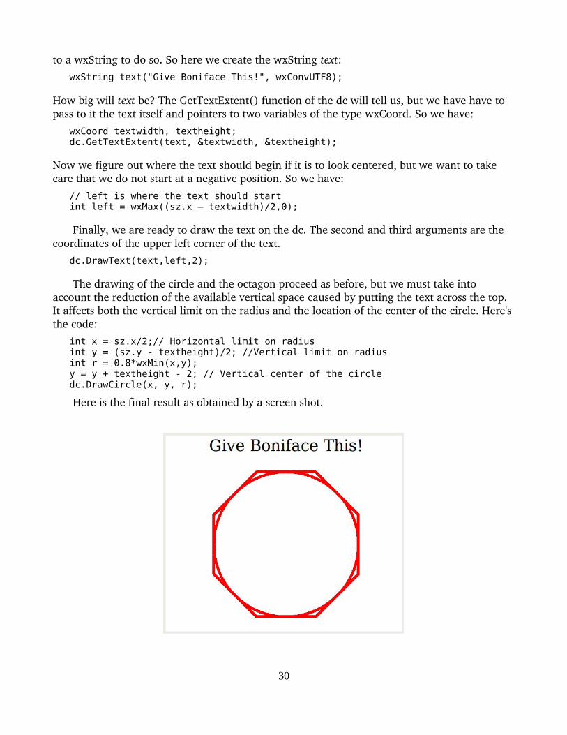
to a wxString to do so. So here we create the wxString text:wxString text("Give Boniface This!", wxConvUTF8);
How big will text be? The GetTextExtent() function of the dc will tell us, but we have have to pass to it the text itself and pointers to two variables of the type wxCoord. So we have:
wxCoord textwidth, textheight;dc.GetTextExtent(text, &textwidth, &textheight);
Now we figure out where the text should begin if it is to look centered, but we want to take care that we do not start at a negative position. So we have:
// left is where the text should startint left = wxMax((sz.x – textwidth)/2,0);
Finally, we are ready to draw the text on the dc. The second and third arguments are the coordinates of the upper left corner of the text.
dc.DrawText(text,left,2);
The drawing of the circle and the octagon proceed as before, but we must take into account the reduction of the available vertical space caused by putting the text across the top. It affects both the vertical limit on the radius and the location of the center of the circle. Here'sthe code:
int x = sz.x/2;// Horizontal limit on radiusint y = (sz.y - textheight)/2; //Vertical limit on radiusint r = 0.8*wxMin(x,y);y = y + textheight - 2; // Vertical center of the circledc.DrawCircle(x, y, r);
Here is the final result as obtained by a screen shot.
30

The final version of Giotto() follows.
void Giotto(wxDC &dc,wxSize &sz){// clear the dc to whitedc.SetBrush(*wxWHITE_BRUSH);dc.Clear();
// Put some text on the screendc.SetTextForeground( *wxBLACK);// Adjust the point size of the font to the height of the windowint PointSize = 0.06*sz.y;//Create a PointSize serif font, that is not bold, not italic, not underlinedwxFont GiottoFont(PointSize,wxFONTFAMILY_ROMAN,wxNORMAL,wxNORMAL,false);// Tell dc to use this fontdc.SetFont(GiottoFont);wxCoord textwidth, textheight;wxString text("Give Boniface This!", wxConvUTF8);dc.GetTextExtent(text, &textwidth, &textheight);// left is where the text should startint left = wxMax((sz.x - textwidth)/2,0);
dc.DrawText(text,left,2);
// Create the color RedwxColor Red(255,0,0);// Create a pen using it, 6 pixels wide and drawing a solid linewxPen myRedPen(Red,6,wxSOLID);// Tell dc to use itdc.SetPen(myRedPen);
int x = sz.x/2;// Horizontal limit on radiusint y = (sz.y - textheight)/2; //Vertical limit on radiusint r = 0.8*wxMin(x,y);y = y + textheight - 2; // Vertical center of the circledc.DrawCircle(x, y, r);//// Draw an octagon around the circle// tangent of 22.5 degrees = .414214;int h = 0.414214*r;
dc.DrawLine(x+r,y+h,x+r,y-h); // right verticaldc.DrawLine(x-r,y+h,x-r,y-h); // left verticaldc.DrawLine(x-h,y-r,x+h,y-r); // top horizontaldc.DrawLine(x-h,y+r,x+h,y+r); // bottom horizontaldc.DrawLine(x-r,y-h,x-h,y-r); // top left slantdc.DrawLine(x+h,y-r,x+r,y-h); // top right slantdc.DrawLine(x-r,y+h,x-h,y+r); // bottom left slantdc.DrawLine(x+h,y+r,x+r,y+h); // bottom right slant}
Saving Graphs as .PNG and .JPG FilesWhen the user closes the GiottoDialog, we will save the drawing to a PNG and to a JPG
file. More correctly said, we will create a memory Device Context (called “memDC”) and a bitmap (called “paper”), assign “paper” to “memDC” to write on, have Giotto draw on memDC,then free “paper” from memDC and save it to a .png (or to a .jpg file). Saving to both types of files was an experiment to look at the size of the file and the quality of the result. The .png file was expected to win, that is, to be smaller and to reproduce better, because, in the words of Wikipedia, “when storing images that contain text, line art, or graphics – images with sharp transitions and large areas of solid color – the PNG format can compress image data more thanJPEG can, and without the noticeable visual artifacts which JPEG produces around highcontrast areas.” Let's see what happens. (PNG stands for Portable Network Graphics and JPEG
31

stands for Joint Photographic Experts Group.)
Because the Giotto program is over in a different .cpp file, we will need a prototype, like this: void Giotto(wxDC &dc,wxSize &sz);
Then the expanded response to the Giotto button click is the following.void GwxFrame::OnGiottoBtnClick(wxCommandEvent& event){
GiottoDialog *dlg = new GiottoDialog(this);dlg->ShowModal();
/* To save our drawing to a file, we first create a bitmap, thena memory DC, then hand the bitmap to the memory DC to use aspaper to draw on, then have Giotto draw on it, then free the
bitmap from the DC and make it write itself as a .png file.*/
// Create a bitmap 400 pixels wide and 430 pixels high.// Call it "paper" because Giotto will draw on it.wxBitmap *paper = new wxBitmap( 400,430);
// Create a memory Device ContextwxMemoryDC memDC;
// Tell memDC to write on “paper”.memDC.SelectObject( *paper );
// Create a wxSize object with the size of “paper”.wxSize sz(400,430);
// Call Giotto to draw on memDCGiotto(memDC,sz);
// Tell memDC to write on a fake bitmap;// this frees up "paper" so that it can write itself to a file.memDC.SelectObject( wxNullBitmap );
// Put the contents of "paper” into a png and into a jpeg file.
paper->SaveFile( _T("Giotto.png"), wxBITMAP_TYPE_PNG,(wxPalette*)NULL );
paper->SaveFile( _T("Giotto.jpg"), wxBITMAP_TYPE_JPEG, (wxPalette*)NULL );
delete paper;}
Click the buildandrun icon, click the Save button. Then start your word processor and insert Giotto.jpg and Giotto.png, as shown below, with the .jpg on the left. I see little difference in the quality of the result. At high resolution in color, there are some black pixels along the edge of the red lines in the Giotto.jpg file which are not there in the Giotto.png file. The Giotto.jpg file, however, is 16.1 kilobytes, while the Giotto.png is only 9.3 kilobytes. So the experiment came out as expected, and we will save Gwx graphs as .png files.
32

At this point, my major questions about the usability of wxWidgets for writing a crossplatform version of G7 have been largely resolved. It can be done. Of course, lots of work remains. Every form displayed by G7 must be rewritten, and there are about twenty of them. The use of grids may prove to be quite different. Various operating system calls will have to be changed. I need to get a better understanding of the debugger under Code::Blocks. And my project to record progress as a sequence of tutorials is going to be time consuming. But I think all this is doable and will give us a firm basis for G in the future.
33

Gwx Tutorial 4: The Debugger, an Improved Chop(), and TextSubstitution
As long as you make no mistakes, you don't need the debugger; but in working on this tutorial, I made a simple mistake which might have held me up for days had it not been for thedebugger. So it's time to have a look at it. We will then refine the chop() routine so that it distinguishes:
numbers (including those in scientific notation) words beginning with a letter but including the digits and $ and _arithmetic operators ( = + * and / ) # and " and other punctuation.
Finally, we will program text substitution, so the %0, %1, %2, … %9 in input lines will be replaced by specified text.
The Code::Blocks Debugger with GNU GCCFor the debugger to work effectively, the program must be compiled with a flag (g) set so
that the compiler generates a symbol table. In Code::Blocks, to set the flag, click Project | Build options … on the main menu. The first option is “Produce debugging symbols [g]”. Be sure that its box is checked, along with that of “Enable all compiler warnings.” Be sure that thebox for “Strip all symbols from binary [s] is NOT checked. Click Build | Rebuild to ensure thatthe entire project has been compiled with these options. After doing this once, it should be sufficient to use just the “build and run” icon as usual.
If you want to have the convenient feature of the the debugger showing the value of an expression when you hover the the cursor over it, you will need to change the default debugger settings. On the Code::Blocks main menu across the top, click Settings. Then click “Debugger settings.” In the white pane on the the left there should be an item “GDB/CDB debugger” with a rightpointing triangle to the left of it. If the word “Default” is not already on the line below, click on the triangle, and the word “Default” should appear below. Click on thisword. Then put a check mark in the box of the option “Evaluate expression under the cursor”. Click OK. Why so important a feature should be so well hidden eludes me.
Another device for showing the values of variables is to set “watches.” To be able to do so, click “Debug” on the Code::Blocks main window; then click “Debugging windows” and check the box for Watches.
Decide where you want a breakpoint and click just a tiny bit to the right of the line number. A red circle should appear.
Start the debugger. Click Debug | Start. The program should run to the breakpoint and put a white triangle inside the red circle. Now click Debug | Edit watches and in the window which comes up, click the “Add” button, and enter the name of the variable you want to watch.You should see its name and current value in the watch window. Or, if you have set up “cursorhovering” you can use it.
Supposedly F8 will start the debugger and F7 will go to the next line of the program, whileF4 will run to the cursor and Shift F7 will step into a function call. In my experience, however,
34
I found it worked best to use Debug | Start to get started and to use Debug | Next line the firsttime I needed the Next line. After that, the F7 worked.
That should get you started. It is a good idea to try this out before you actually need it. The maintainers of Code::Blocks say that the “nightly builds” since 10.05 are a big improvement in the debugging area. I have not tried them.
Refining chop() In the second tutorial, we introduced a simple version of chop(0) to illustrate the
interaction of (1) the user's entering a line in the Command Box and tapping the Enter key (2) the gselect() routine, and (3) the chop() routine. That version of chop() recognized only spaces and tabs as separators of components in the line. G requires a more sensitive division. The prototype for chop() is
char chop(char *s);
where s is a pointer to space where chop can put nullterminated cstring. Thus, two things are returned by chop: (1) the value of the function and (2) the contents of string pointed to by s.
Here is an example of how it should chop up a line.
Line: f abc=2.5*(ghi+jkl)
Successive calls to chop() should return:
value of function: a a = n * ( a + a ) e
string in s[] : f abc = 2.5 * ( ghi + jkl )
The string in s[] is always a proper, nullterminated C string.
Any string beginning with a letter returns the character 'a' as value of the function and the characters in s[] should extend until something other than a letter, a digit, a '.', '$' or a '_' is encountered. These strings are typically G commands or variable names, which must begin with a letter but may include digits and '$', '_', and '.' characters. Any other character breaks the buildup of the string and causes chop() to return.
Any string of characters beginning with a digit returns as value of the function the character 'n' (for number) with the number as an ASCII string in s[]. This string may include, besides digits, a '.' and the expressions E+ and E to allow for scientific notation of numbers – e.g. 2.72E+05. The string extends until a character other than a digit, a '.', or E+ or E is encountered, whereupon chop() returns.
Spaces and tabs break the build up of the type 'a' and type 'n' strings, but are then just “eaten up” by chop() which passes on looking for some other kind of character.
A string of characters beginning with a quotation mark, " , returns the " as the value of the function and everything inside the quotes – but not the quotes themselves – in s[]. These may be titles for graphs or regressions.
A string of characters beginning with a # returns the # as the value of the function and the # and everything following it on the line in s[]. Essentially, the # and everything following
35
on the line will be considered a comment. These characters will be shown on the Results screen, but not considered a command.
A null – the '\0' at the end of a line – breaks off and returns any string that was being built and then, on the next call, returns 'e' for End of Line.
Any other character – and these include = + * / ( ) [ ] – returns the character itself as the value of the function and as the content of the string in s[]. More precisely, s[] will have the character in position 0 and '\0' in position 1.
Here is a chop() which does all this. Note that the value of the function, chopreturn, is set as soon as the type of string is known. Then, when we hit the end of the string, we just do
return chopreturn;
Among the #include statements near the top of GwxMain.cpp we need to have:
#include <ctype.h>
for the use of the isalnum() and isdigit() functions.
char chop(char *s){ short i; unsigned short cu; i = 0; char chopreturn = 'a';
while(i < MAXLINE){ cu = *pinbuf++;
// Is it a space or tab? if(cu == ' ' || cu == '\t'){ // found a space or tab if(i== 0) continue; // eat up white space s[i] = '\0'; // end the word being returned return chopreturn; }
// Is it an End of line if(cu == 0){ // found an end of line s[i] = '\0'; // end the word being built if(i > 0) { // if a word has been started pinbuf--; // back up one character
// so the EOL will be read next time return chopreturn; // return the word that had been started } else return 'e'; }
// Is it a number? if(i == 0 && (isdigit(cu) || cu == '.')){
// found a digit or decimal point chopreturn = 'n'; s[i++] = cu; while(isdigit(*pinbuf) || *pinbuf == '.' || *pinbuf == 'E' // allow for scientific notation
36
|| (*pinbuf == '+' && s[i-1] == 'E') || (*pinbuf == '-' && s[i-1] == 'E')){ s[i++] = *pinbuf++; } s[i] = '\0'; return chopreturn; }
// Is it a string in quotes? if (i == 0 && cu == '"'){ // Found something in quotes chopreturn = '"'; while(*pinbuf != '"' && *pinbuf != '\0'){ s[i++] = *pinbuf++; } s[i] = '\0'; return chopreturn; }
// Is it a # ? If so, the rest of the line is a comment if (i == 0 && cu == '#'){ chopreturn = '#'; s[i++] = '#'; while(*pinbuf != '\0'){ s[i++] = *pinbuf++; } s[i] = '\0'; return chopreturn; }
// Is it a letter? if(i == 0 && (isalnum(cu))){ chopreturn = 'a'; s[i++] = cu; while(isalnum(*pinbuf) || isdigit(*pinbuf) || *pinbuf == '.' || *pinbuf == '_' || *pinbuf == '$' ){ s[i++] = *pinbuf++; } s[i] = '\0'; return chopreturn; } // Operators and other punctuation s[i++] = cu; s[i] = '\0'; chopreturn = cu; return chopreturn; } // Should not get here, but if we do s[MAXLINE-1] = '\0'; return ERR; }
Replace the previous chop() with this one and test it out. It may have to undergo modification later, but right now it seems to work well and is reasonably simple.
37

Making Text SubstitutionsOne of G's most useful abilities is text substitution. When it is executing an “add” or “fadd” file,it may come upon the symbol %0 or %1, or %2 and so on up to %9. These symbols indicate that previously established text strings should be substituted for these symbols in the input line. For example, if %0 has been defined as Aaa and the command
f %0 = x + y
is given, chop() will see the command as
f Aaa = x + y
The current coding in G7 is rather complex, and I want to try something much simpler as shown here.
First of all, we have to reserve some space for storing the ten possible strings to be substituted. We will do it right along with the reservation of space for inbuf and inbufAsRead.#define MAXPRINTOUT 500#define MAXLINE 500#define MAXSUBSTITUTES 100 //Maximum length of any one susbstitute string#define OK 1#define ERR -1
char printout[MAXPRINTOUT], inbufAsRead[MAXLINE], inbuf[MAXLINE], *pinbuf;char substitutes[10][MAXSUBSTITUTES];
We also need to get some text into at least the first two rows of the substitutes array so we can test our program for making the substitutions. In the current G7, this step is usually done by arguments on an add command or from the argument file of a fadd command. We don't have that machinery set up yet for Gwx, so – just for testing the substitution code – we will initialize the first two rows of substitutes when the GwxFrame is created, like this:void GwxFrame::OnCreate(wxWindowCreateEvent& event){ printout[0] = '\0'; // Just for testing substitutes strcpy(substitutes[0],"Aaa"); strcpy(substitutes[1],"Bbb"); }
Now we turn to what is done in OnCmdBoxTextEnter right after the user types something and taps the Enter key. This is where the substitution is actually done. Here is the code, with the new part in bold.
void GwxFrame::OnCmdBoxTextEnter(wxCommandEvent& event){ wxString textFCB = CmdBox->GetValue(); CmdBox->Insert(textFCB, 0); CmdBox->SetValue(wxT("")); if(CmdBox->GetCount() == 10) CmdBox->Delete(9); Results->AppendText(textFCB); Results->AppendText(_("\n")); // Put what was read from the CmdBox into inbufAsRead as a standard C string strncpy(inbufAsRead,(const char*) textFCB.mb_str(wxConvUTF8),MAXLINE-1); // Copy inbufAsRead into inbuf with text substitution. short i,j, srow, scol; i = 0; j= 0; srow = 0; scol = 0; // i keeps track of where we are in inbufAsRead.
38

// j keeps track of where we are in inbuf. while(inbufAsRead[i] != '\0'&& j < MAXLINE && i < MAXLINE){ // check for text substitution signals: %0, %1, %2 etc. if(inbufAsRead[i]== '%' && isdigit(inbufAsRead[i+1])){ // make text substitution srow = inbufAsRead[i+1]-48; //'0' is ASCII 48 i += 2; scol = 0; while(substitutes[srow][scol] != '\0' && j < MAXLINE &&
scol < MAXSUBSTITUTES){ inbuf[j++] = substitutes[srow][scol++]; } } else inbuf[j++] = inbufAsRead[i++]; } if(j >= MAXLINE) { printg("%s\n","That line was too tong!"); j--; } inbuf[j] = '\0'; pinbuf = inbuf; gselect(); }
With the comments, the program is pretty selfexplanatory. The string inbufAsRead is what was read from the command box. The string inbuf is inbufAsRead expanded by replacing %0, %1, etc. by the appropriate text strings.
The line srow = inbufAsRead[i+1]-48; //'0' is ASCII 48
perhaps needs a word of explanation. The ASCII character in inbufAsRead[i+1] will be a 0, or a 1, or a 2, … or a 9. The numeric values of these ASCII characters are 48, 49, 50, etc., so by subtracting 48 we get the numeric value of the row in substitutes. Perhaps it would be better practice to use the atoi() function to do the conversion, but the result would be the same.
In my testing of it, this code works fine and is much simpler than what I and others wrote for G7. It is perhaps more extravagant with space than I would have dared to be back in the days of DOS and the 640 kilobyte limit on programs.
39
Tutorial 5: Making printg() Global.Back in Tutorial 1, when we introduced the printg() function, we made it a member of the
GwxFrame class, the class I think of as the interface, the class which puts on the screen the form with the command box and the Results area for displaying output text. By doing so, we saved ourselves some complexity at the time and could concentrate on printg(), which had enough complexity. But as we now go further, the decision to make it a member function would soon come back to haunt us. Every time we wanted to print “Hello!” from a function that was not a member of the interface class, we would have to write something like
MainFrame>printg(“Hello!\n”);
instead of just
printg(“Hello!\n”);
Worse still, the value of MainFrame was created as a local variable and would not be available,so essentially our printg() is usable only from members of the interface class. That is too limiting. We need for printg() to be available everywhere.
The first step in the solution to this problem is to make printg() a “friend” rather than a member of the interface class. So edit GwxMain.h and changeclass GwxFrame: public wxFrame{ public:
GwxFrame(wxWindow* parent,wxWindowID id = -1); virtual ~GwxFrame(); void printg(char *fmt, ...); short gselect();
to
class GwxFrame: public wxFrame{ public:
GwxFrame(wxWindow* parent,wxWindowID id = -1); virtual ~GwxFrame(); friend void printg(char *fmt, ...);
Notice both the “friend” keyword and the fact that all reference to gselect() has been removed.It needed to be in the class only because it used printg(), but printg() is going global.
Now let's look at printg() itself. It needs the following code#define MAXPRINTOUT 500#define MAXLINE 500#define MAXSUBSTITUTES 100 //Maximum length of any one susbstitute string#define OK 1#define ERR -1
char printout[MAXPRINTOUT], inbufAsRead[MAXLINE], inbuf[MAXLINE], *pinbuf;char substitutes[10][MAXSUBSTITUTES];
void printg(char *fmt, ...){ char buf[MAXLINE]; va_list args;
40
va_start(args, fmt); vsprintf(buf, fmt, args); va_end(args);
short lenb, lenp; lenb = strlen(buf); lenp = strlen(printout); if(lenb+lenp >= MAXLINE-2){ wxString wxPO(printout, wxConvUTF8); MainFrame->Results->AppendText(wxPO); printout[0] = '\0'; } strcat(printout, buf); lenp = strlen(printout); // If the last character in printout is \n, then it is time to // print if(printout[lenp-1] == '\n'){ // convert printout to a wxString, which we will call wxPO wxString wxPO(printout, wxConvUTF8); MainFrame->Results->AppendText(wxPO); printout[0] = '\0'; } }
The only changes in the whole routine are, first, to changevoid GwxFrame::printg(char *fmt, ...){
to void printg(char *fmt, ...){
and to insert MainFrame> in front of Results in two places. But what is this MainFrame business? MainFrame is the pointer to our interface class.
Open the file GwxApp.cpp; use File | Open to do so. You will seebool GwxApp::OnInit(){ //(*AppInitialize bool wxsOK = true; wxInitAllImageHandlers(); if ( wxsOK ) { GwxFrame* Frame = new GwxFrame(0); Frame->Show(); SetTopWindow(Frame); } //*) return wxsOK;}
See that variable Frame? That is the precious pointer to our interface class. But it is a local variable and we need to use it elsewhere. So we need to make it a global variable. And in the process, let's give it a more distinctive name, like MainFrame. The code we want is:IMPLEMENT_APP(GwxApp);
GwxFrame* MainFrame;
bool GwxApp::OnInit() { //(*AppInitialize bool wxsOK = true; wxInitAllImageHandlers(); if ( wxsOK ){ MainFrame = new GwxFrame(0);
41
MainFrame->Show(); SetTopWindow(MainFrame); } //*) return wxsOK; }
Note that MainFrame is now a global variable. Note further that we do NOT have GwxFrame* MainFrame = new GwxFrame(0);
That would have created a second MainFrame variable, this one local, and it would have hidden the global MainFrame variable. (I made this mistake.)
Now that we have made MainFrame a global variable in GwxApp.cpp, we need to let printg() over in GwxMain.cpp know about it. So just above the code for printg(), we insert the line
extern GwxFrame* MainFrame;
Finally, since gselect is no longer a member of the interface class, we need to change its the top line of its code fromshort GwxFrame::gselect(){
to justshort gselect(){
Make all of those changes and, if I have not forgotten to tell you something I did, you should be able to compile and run and get a Gwx that seems to work just like the version at the end of the previous tutorial. The difference, however, is enormous. We can now go forward with introducing the various functions of Gwx without having to make them all members of the interface class just to use the printg() function.
Picking the Starting DirectoryWord processor and spread sheet programs can start and do a lot of work without any
reference to a particular directory (also called folder) on the hard disk. Only when it comes time to save the document or spreadsheet do you have to pick a directory on the hard disk in which to save it. Of course, if the document already exists on the hard disk and you want to open it to work further on it, then you have to search the hard disk for it from the start of yoursession.
G, however, always needs a foothold on the hard disk before it can do anything useful. That is because it must establish a workspace data bank on the hard disk before it can introduce data, and it has to have data before it can do any real work. G for Windows creates the workspace from information in a file, always called g.cfg, in the directory where it starts. We want Gwx to work in the same way, but there is a problem: How do we tell Gwx in which directory to look for the g.cfg file? We need for Gwx to open a directorypicking dialog. Since the “Miranda” button has served its purpose of testing printg(), we can relabel and reprogram it to open the directory picker. You can easily change its label property from “Miranda” to “Pick Dir”. Then reprogram what the button does as follows.#include <wx/dirdlg.h>
42
void GwxFrame::OnMirandaBtnClick(wxCommandEvent& event){ printg("%s", "O brave new Gwx!\n"); wxString defaultPath = wxT("/home"); wxSize DirPickerSize(400,400); wxPoint DirPickerPosition(100,100); wxDirDialog dialog(NULL,wxT("Pick the Directory in Which to Start Gwx"), defaultPath,wxDD_DEFAULT_STYLE | wxDD_CHANGE_DIR, DirPickerPosition,
DirPickerSize); if(dialog.ShowModal() == wxID_OK){ wxString path = dialog.GetPath(); printg("Gwx will start in: %s \n",(const char *)path.mb_str(wxConvUTF8)); } else printg("Starting directory not established.\n"); CmdBox->SetFocus(); }
The central statement here is:
wxDirDialog dialog(NULL,wxT("Pick the Directory in Which to Start Gwx"), defaultPath,wxDD_DEFAULT_STYLE | wxDD_CHANGE_DIR, DirPickerPosition,
DirPickerSize);
which is the wxWidgets special function for displaying a directorypicking window. The first argument in the call is the parent. I saw examples with both “this” and “NULL” as this first argument. It seemed to work the same both ways, so I left the NULL. The second argument is what will appear as the title in the top bar of the frame around the window. It must be a wxString variable; hence the wxT(“...”).
The third argument is the path to the directory in which the window opens. It is here called “defaultPath”, but notice that just above this variable has been define by
wxString defaultPath = wxT("/home");
so the directory picker will open in the /home directory. A fellow named Peter may say, “It is certain that the directory I want will be NOT be in /home; the only directory there is peter. Thehighest directory with any chance of being the one I want is in /home/peter. Why can't the program start by looking in /home/peter?” I think the answer to petulant Peter is fairly clear. There may be more than one directory directly under /home, and even if there is only one, I know of no way to detect this fact and to open in it rather than in /home. That is not to say it cannot be done, but I don't how. And certainly, not everyone has a /home/peter directory.3
This line seems to me to be inevitably dependent on the operating system. On a Windows system, we would probably want to start with “c:” and the directory we are looking for would be one of those directly under c:, say c:\quest.
The next argument in the wxDirDialog dialog() construction statement is the style argument. As is common in wxWidgets, a number possible style features are combined with the or operator. Each feature is indicated by a 1 bit at a particular place in the byte which specifies the style. So our style,
wxDD_DEFAULT_STYLE | wxDD_CHANGE_DIR
3 There is a good reason why Linux has these “user name” directories directly under /home. Linux, is designed to look like Unix, which is a time-sharing operating system with a number of users, each of whom has a directory under the /home directory. As a single-user system, Linux generally has only one directory under the /home directory, and it is given the name of the user.
43

is the standard (or default) style, plus a change of directory into the one selected.
The next two arguments are the position and size of the directorypicker window. I have tried to follow the directions in the official wxWidgets documentation, but seemingly without effect. The window opens occupying the full screen. The documentation notes that these arguments are ignored in Windows. Apparently they are also ignored in Ubuntu Linux.
Next, we show the dialog modally, that is, so that nothing else can be done until the user closes the dialog. So let us suppose that our user searches about, finds the directory he wants, puts the selection bar on it and clicks the “Open” button in the lower right corner. The windowwill then close and return the value wxID_OK. So we test to see if that is the value returned. If so, we use the GetPath() function of the dialog to ask it what directory the selection bar was on when the dialog closed. That gives us the path to the directory where Gwx is to put its workspace bank and possibly, in due course, to open one or more assigned banks. That path will be a wxString in UTF8 Unicode, not a standard nullterminated C string such as printg() can display. So we have to convert it. Here is the code for all of this.
if(dialog.ShowModal() == wxID_OK){ wxString path = dialog.GetPath(); printg("Gwx will start in: %s \n", (const char *)path.mb_str(wxConvUTF8)); }
Getting the string conversion to work took me longer than all the rest.
There is, of course, the possibility that the user did not click the OK button but the Cancel button instead. We simply report that fact on the screen with the line else printg("Starting directory not established.\n");
When the program was run with just this much of the code in place, that is, without the last line
CmdBox->SetFocus();
it ran all right; but when it finished, the Command Box had lost the insertion point cursor, blinking vertical bar. The index of the Smart and Hock book (cited on page 8) makes no mention of “focus” or “SetFocus”. There were some mentions on the Internet, mainly complaining that it didn't work. But I decided to try it, and it did work!
The next thing we need to do is to look in the directory which has been selected for a g.cfgfile to tell us how to define the workspace bank and then to create the bank accordingly. Alternatively, if there is no g.cfg file in the chosen directory, we need to create one. But first, we need to learn about G workspace banks. And that subject takes us into the next tutorial.
Saving and Moving the Gwx Program and Project to Other ComputersAt this point, it occurred to me that I should backup the Gwx directory to a USB flash drive
and try to install it on another Ubuntu Linux computer. I put in a USB drive and “dragged” the Gwx directory onto it. To test it out, I then opened a terminal window, did
cd /medials
and saw that I had in /media a directory called 00477E64. That had to be the USB drive, so I
44

didcd 0*
That was enough to move me to the USB drive. There, with a sequence of ls and cd commands I arrived at the directory /Gwx/bin/Debug, where I saw a file Gwx. I did “ls l” and saw that it had x permissions, that is to say, it was executable. So I did
./Gwx
and it executed just fine. So then I took the USB drive over to another computer, found the Gwx file, but it had lost its x permissions and would not execute. I tried “chmod a+x Gwx” to no avail. At the suggestion of someone else, I copied on this machne Gwx from the USB drive to the hard disk and there did the chmod, and it worked. I then put the whole project on the second machine's hard disk and used Code::Blocks to rebuild it. That worked. I copied the executable Gwx so created from the hard disk to the USB drive, but on the USB drive it had lost its x permissions. I then took the USB drive over to the first machine and, lo, the Gwx file had x permissions and executed fine! Thus, one machine allows x permissions on the USB drive and the other does not. Strange. The only software difference that I can think of betweenthe two is that the first machine has a dual boot with Windows, while the second has only Linux. But with a little patience, the program will build and run on both machines.
Later, I took the USB drive to yet a third computer with a dual boot of Ubuntu Linux and Windows. I booted Linux, put in the USB drive, opened a terminal window, navigated to the USB drive and found that Gwx indeed had x permissions and ./Gwx worked immediately.
Looking back at this paragraph a year or two after it was written, I am surprised that the program worked at all on the USB file. In general, these drives and external hard drives come with some file system comprehensible to Windows. These file systems generally do not accommodate the Linux permissions, so chmod is ineffective on them. However, the file can becopied to the Linux partition of the hard disk of a machine that has Linux installed, chmod applied, and the file will execute.
When I copy the whole of Gwx from an external drive, I then click the “Build” icon and recompile the whole thing. It then usually works smoothly.
The Road AheadAt this point, we could probably successfully dump large amounts of G7 code into Gwx.
When we get to the algorithms, like regression, we will probably do just that, but at this point Iwant to explain carefully from the ground up how G works. So we will go slowly and add a little at a time.
Before G can do anything useful, it must have a workspace bank. The next tutorial explainsin detail the structure of such a bank. Gwx will use exactly the same structure for these banks as does G7. When G7 starts, it reads a configuration file and, using information from that file creates a workspace bank. Gwx will work similarly. But whereas G7 looks for a file named g.cfg, Gwx will look for Gwx.cfg. The click of a button will allow the user to navigate to the directory (= folder) where the Gwx.cfg file is, along with data banks, command files, and result files for a particular modelbuilding project.
45

This file will be simpler than the g.cfg file. It will have only the beginning year of the workspace bank, the maximum number of observations in any series, the default frequency of the bank, and an optional name of a file of G commands to be executed before any commands are taken from the user. The Gwx.cfg file will be read from the starting directory immediately after picking this directory.
The workspace will then be created and some series put into it. The reason for having the program put these series into the bank is that we can then develop the “type” command and have something to test it on. Once that is working, we will need to deal with handling dates. Then we can develop the “data” command to get data into the workspace. Next, comes the “add” command to take commands, including the “data” command, from a file.
At that point, a lot lies open. Probably coding the “f” command to form a new variable from existing ones by a formula is most important. Then we can add the “bank” command to connect to an existing data bank. Drawing and saving graphs may come next, then regression, then VAM files and the “show” command. At that point, we can return to other forms of data entry and other types of banks and other algorithms and matrix algebra. Finally, will come building and running models from inside Gwx.
46

Tutorial 6: A Data Bank for GwxIn this tutorial, we will add code to create a workspace bank, to add a series to it, to
extract a series from it, and to display that series numerically via the printg() function. These functions will then be tested by putting into the bank at the time it is created three series and then having the user use the type command to display them.
Structure of the Standard G Data BankG7 for Windows has four types of data banks: the standard G bank, the compressed bank,
the hashed bank, and the VAM file. The first three may all be called the scalar banks; they all handle time series of a single number, a scalar, such as GDP, the unemployment rate, or the LIBOR interest rate. The VAM file handles time series of vectors and matrices. In this tutorial, we will be concerned only with the first, the standard G bank. Among the scalar banks, only it can be used as the workspace of G. The other two scalar types contain the same sort of information as does the standard bank but in a more compressed form. The hashed bank, moreover, can have far more series than can either the standard or the compressed bank. But neither the compressed nor the hashed bank can grow dynamically as G runs. They cannot addseries or extend existing series. They are great for holding a fixed body of data, say the National Accounts of the United States from 1945 to 2012, but cannot be used as the G workspace, which must be capable of adding and extending series. So we shall be concerned inthis tutorial only with the standard bank. At the end of the tutorial, I will add a few words about the ideas used in the compressed and hashed banks.
A standard G bank consists of two files, the index file and the bank file. The root name of the two is identical, but the name of the index file has the extension .ind while the extension ofthe bank file is .bnk. For example, the names of the two files for the Quarterly Income and Product accounts are quip.ind and quip.bnk. Every series has exactly the same amount of spacereserved for it in the bank file. The bank file begins with the content of this header:#define MAXBANKTITLE 80struct bnkHeader {
short jahra; // base year of all series in bankshort stper; // starting period within base year, usually 1short nobs; // number of observations for which space is reserved.char bnktitle[MAXBANKTITLE]; };
Since each of the three shorts occupies 2 bytes and the bnktitle takes 80 bytes, the total space occupied by the header is 86 bytes. (The names of the variables are no longer what I would regard as optimal but are retained to facilitate comparison with G7. The name jahra, forexample, is left over from G's predecessor, LS, which was written in Fortran, where variables beginning with i, j, k, l, m, and n were automatically integers. So we wanted a name meaning year but beginning with one of these letters. The German word Jahr came immediately to mind, and the first year could be jahra.)
After the header come the data time series, each preceded by its frequency as a 1byte char variable with a value of 1 for annual series, 4 for quarterly series, and 12 for monthly series. Observations before or after the available data are filled with MISSING, which has a
47

numerical value of 1/1048576 or approximately 0.0000009537, which seems a highly unlikely value for a true observation. It is not, however, a number chosen on a whim. The 10485676 is a power of 2, namely the 20th. Thus this value of MISSING can be represented exactly in the computer's internal binary representation of numbers. We will return to this point in the 10th tutorial.
For example, suppose that jahra is 1990 and we have data for unemployment beginning in 1991. The annual value for 1991 is 5.5, the quarterly values are 5.5, 5.0, 5.5, and 6.0, and the monthly values are 5.6, 5.5, 5.4, 5.3, 5.0, 4.7, etc. Then data the three series for the two years, 1990 and 1991, would appear as shown in the table on the left.
This system can be wasteful of space, especiallywhen handling series of different frequencies. Eliminating that waste is part of what the compressed bank is about. On the other hand, if the data is all or nearly all of the same frequency and covering the same period, as is often the case, the waste is minimal.
If we get additional data points at the beginning or end of the series, we have places to put them so long as they do not fall outside the space reserved for the series. To continue our example, if nobs in the header is 120, the bank can accommodate an annual series stretching from 1990 to 2109 (120 annual observations) or quarterly data from 1990 through 2019 (120 quarterly observations) or monthly data from 1990 through 1999 (120 monthly observations).
The other piece of a standard G bank is the index file. It begins with a twobyte short, nseries, the number of series in the bank, followed by (a) an array, called indx, of nseries+1 unsigned shorts (whose values I will explain in a moment) followedby (b) the names of the series (such as gdp, unemp,rtb) separated by nulls, the '\0' character. These
names are all considered as one, possibly very big, onedimensional array called names. If our bank has precisely the three variables just named, then the names array would be:
gdp0unemp0rtb0
where a 0 represents the '\0' or NULL character. The nseries+1 unsigned shorts in the indx array are the position of the first letter of the name of each series in the names array. For this
48
1 4 12
MISSING MISSING MISSING
5.5 MISSING MISSING
MISSING MISSING
MISSING MISSING
5.5 MISSING
5.0 MISSING
5.5 MISSING
6.0 MISSING
MISSING
MISSING
MISSING
MISSING
5.6
5.5
5.4
5.3
5.0
4.7
etc.
example, the indx array would be 0, 4, 10, 14. The final value – 14 in the example – is where the name of series number nseries+1 would begin.
The usefulness of the indx array becomes apparent from the findname function, which returns the position of a given name, gname, in the names array and thus tells us where to find the data for the series in the bank file./* findname -- finds position of given name, gname, in the names array. */ long findname(char *gname){
long i; for(i=0;i<nseries;i++)
if(strcmp(gname,&names[indx[i]])==0) return(i); return(-1); }
(The standard C string compare function, strcmp(), returns 0 if the two argument strings are the same.)
It may seem pointless to store the indx array on the hard disk, since it could be easily reconstructed from the names array (and the total number of characters in it) every time the bank is assigned. However, storing the indx array consumes little disk space and has the advantage of compatibility with other versions of G.)
How Many Names Are Possible?
The names array is limited to a total of NCMAX characters, counting the nulls. In G7 for Windows, NCMAX is currently set to 65535, the largest number that can be represented by an unsigned short. NSMAX is set to the same value, but clearly the NCMAX constraint is binding. With variable names averaging 9 characters plus the nul, there would be room for 6,553 series.That is enough for much work. For larger data collections, the hashed bank offers the possibility of handling millions of series.
In working with a standard bank, G reads the entire names and indx arrays into memory from the .ind file on the hard disk. When asked to find the values for a certain variable, say gnp, it uses the findname() function shown above to find it; the series's number returned by that function then tells the program where to look for the series in the array of data in the bank file. The program then plucks out that series from the bank file, which remains on the hard disk. Neither file is larger than necessary to accommodate the number of series actually inthe bank.
The great advantage of this file structure is that series can easily be added and data for an existing series can be revised or extended, within the limits of the bank. The compressed bankstake less space, and the hashed banks take less space and can handle many more series. But they are static. There is no provision for adding, correcting, or extending a series. If that needs to be done with one of these banks, the bank has to be constructed again from scratch.
Normally, the entire index file is written to the hard disk every time a series is added to the bank. If many series are being added at once, all that writing can be timeconsuming, so G provides the ability to turn off the writing, add all the series, and then turn the writing on again.
49

How many series can one of these banks hold? Since indx is an array of unsigned shorts, the biggest number that one of its cells can hold to is 65535. That then provides an upper bound for the total number of characters in the names array. What is the upper limit on how many series can be given distinct names with 65535 characters? With 2 bytes per name, we can get 52 distinct, onebyte names: A, B, C, … Z, a, b, c, …, z. (Remember that each name must end in a null.) and these names consume 104 bytes. With three bytes per name, we can form 64 names from each of the original by inserting an A, B, …, z, 0, 1, …, 9, $, _ as the second character. That is a total of 52*64 = 3328 names consuming 9984 bytes. That leaves 55447 bytes for names with three letters (four bytes). That is enough for only 13861 of these names, of which there are many more. Thus, the most names we can possibly accommodate is 52+3328+13861 = 17241. That is an absolute maximum on the number of series a standard bank can accommodate. In fact, it is highly improbable that any user would pick names in suchan efficient way, so in practice we should not expect these banks to hold more than 5 or 6 thousand series. The 17241 number, however, is important for our program. If we use it for the maximum number of series, we need not be continually checking in the program to be surethat we are not getting too many series. The constraint on the total number of characters in the names will stop the growth of the bank (probably long) before the limit on the number of names is reached.
Dividing Gwx into Modules and Common.hUp until now, we have put all of our new code into the files created by wxSmith. Gwx,
however, is going to grow quite large, so we need to add separate .cpp files with closely related parts of the program. This division into “modules” speeds compiling of the program because only modules which have been changed since the last compilation need to be recompiled. Also, some testing of GCC indicates that compilation time seems to grow approximately with the square of the size of the module. We will put most of our new code introduced in this tutorial into a file we will call bank.cpp. But we need to let routines in other modules know about those routines by putting their prototypes in a header file which will be “included” in other modules. We will put into that file also the global variables and remove them from GwxMain.cpp. We will call that file common.h. Here is our initial version of it:
/* COMMON.HThis file declares many global variables. It can be "included" into any module of G.In the GwxMain.cpp program, a global variable, say feedchar, should be declared thus:
int feedchar;In all other modules, it should be declared
extern int feedchar;How do we get the "extern" when we need it and avoid having it when itmust not be there? We declare "feedchar" in this file (common.h) as
GLOBAL int feedchar;In GwxMain.cpp program, the inclusion of this file will be preceded by definingGLOBAL as nothing, thus
#define GLOBAL#include "common.h"
In all other programs, we omit the first statement. The lines in common.h#ifndef GLOBAL#define GLOBAL extern#endif
will then define GLOBAL as "extern" so thatGLOBAL int feedchar;
will look to the compiler like
50
extern int feedchar
This problem does not afflict prototypes and defined constants.
It should be noted that this problem was not part of the original C language as presentedin K&R and did not arise when using the DeSmet compiler, which was smart enough toput in one and only one version of a global variable. The "extern" was unnecessary.*/
#ifndef common_h#define common_h#endif
#ifndef GLOBAL#define GLOBAL extern#endif
// Constants#define MAXPRINTOUT 500#define MAXLINE 500#define MAXUNSIGNEDSHORT 65535#define MAXNAMES 17100#define MAXSUBSTITUTES 100 //Maximum length of any one susbstitute string#define NOMAX 600
#define OK 10#define GO 0#define ONCE 1#define STOP 2#define YES 1#define NO 0#define ESC 27#define ERR (-1)#define TRUE 1#define FALSE 0#define SMALL (1.0e-7)#define MISSING -.000001
// Global variablesGLOBAL char printout[MAXPRINTOUT], inbufAsRead[MAXLINE], inbuf[MAXLINE], *pinbuf;GLOBAL char substitutes[10][MAXSUBSTITUTES];GLOBAL char names[MAXUNSIGNEDSHORT];GLOBAL unsigned short indx[MAXNAMES];GLOBAL short jahrba, nobs, nopy, nobs_ws, freqdefault;GLOBAL unsigned short nseries;GLOBAL FILE *pbank, *ipbank; //for the workspace ws.bnk and ws.ind files
#if !defined(BNKHEADER)#define BNKHEADER 1struct bnkHeader {
short jahra, stper, nobs;char bnktitle[80];};
#endif
// prototypes// In GwxMainvoid printg(char *fmt, ...);short typecmd();
// In bank.cppshort addseries(char *nam, float *series, short nopy, char wrindex_flag, short SeriesLength);short windex(void);short rindex(void);long findname(char *gname);short getseries(char *nam, float *ss, short SeriesLength);
51
//******************************************************************************************
The long comment at the beginning of common.h is extremely important and should be fully understood. Near the top of GwxMain.cpp we now put#define GLOBAL#ifndef COMMON#include "common.h"#endif
Creating a Workspace BankIn this tutorial, we will add code to create a workspace bank, to add a series to it, to
extract a series from it, and to display that series numerically via the printg() function. These functions will then be tested by putting into the bank at the time it is created three series and then having the user use the type command to display them.
The first series we put into the bank, called timea, is a time variable for annual observations. Thus, if 1970 is the beginning of the bank, timea will be:
1970 1971 1972 etc.
The second variable, timeq, will be a time variable for quarterly data. Its values will be:1970.00 1970.25 1970.50 1970.751971.00 1971.25 1971.50 1971.75 etc.
The third variable, timem, will be a time variable for monthly data; its values will be:1970.00 1970.083 1970.167 1970.25 1970.333 1970.4171970.50 1970.583 1970.667 1970.75 1970.833 1970.917 etc.
Here is the code we now add to OnMirandaBtn Click:void GwxFrame::OnMirandaBtnClick(wxCommandEvent& event){ FILE *config = NULL; char s[100]; // for getopt short i;
// . . . . Previously explained code for picking the opening directory remains here.
// Read the Gwx.cfg file
if((config = fopen("Gwx.cfg","r")) == 0){ wxMessageBox(wxT("There must be a Gwx.cfg file in the starting directory."),wxT("Fatal Error"), wxOK,this); return;
} /* The Gwx.cfg File looks like this: Base year of workspace bank; 1970 Maximum number of observations per series; 400 Name of assigned bank; quip.bnk Default frequency: 4 */ // Get base year of the workspace
//The getopt function will be explained below. if(getopt(s,config) == OK) jahrba = atoi(s); // Base year or workspace else { wxMessageBox(wxT("Could not read base year."),wxT("Fatal Error"),wxOK,this); return; }
52

if(getopt(s,config) == OK) { nobs_ws = atoi(s); nobs = nobs_ws; } //Max number of observations else { wxMessageBox(wxT("Could not read Max observations."),wxT("Fatal Error"),wxOK,this); return; } if(getopt(s,config) == OK) freqdefault = atoi(s); //Default frequency else { wxMessageBox(wxT("Could not read default frequency."),wxT("Fatal Error"),wxOK,this); return; } fclose(config);
// Create and load a bnkHeader struct. bnkHeader Hdr; Hdr.jahra = jahrba; Hdr.nobs = nobs_ws; Hdr.stper = 1; strcpy(Hdr.bnktitle, "Untitled");
// Create the workspace bank with no series in it. pbank = fopen("ws.bnk","w+b"); ipbank = fopen("ws.ind","w+b"); if (pbank == 0 || ipbank == 0){ wxMessageBox(wxT("Could not create workspace bank"),wxT("Fatal Error"),wxOK,this); return; } // Write the header to the .bnk file if(fwrite( (void*)&Hdr,sizeof(Hdr),1,pbank)==0){ wxMessageBox(wxT("Could not write header to ws.bnk."),wxT("Fatal Error"),wxOK,this); return; } // write the number of series to the .ind file nseries = 0; if(fwrite(&nseries,sizeof(unsigned short),1,ipbank)==0){ wxMessageBox(wxT("Could not write nseries to ws.ind."),wxT("Fatal Error"),wxOK,this); return; }
// Make up three "time" variables, and put them into the bank.
float *series = new float[nobs_ws]; //First, the annual variable, timea. series[0] = jahrba; float increment = 1.0; for (i = 1;i < nobs_ws; i++){ series[i] = series[i-1] + increment; } // Put it into the workspace; here is the first line of addseries: // short addseries(char *nam, float *series, short nopy, char wrindex_flag, short SeriesLength) // addseries() is in bank.cpp short seriesnum = addseries("timea", series, 1,'y',nobs_ws);
// Now make up and add to the bank the quarterly, timeq series[0] = jahrba; increment = .25; for (i = 1;i < nobs_ws; i++){ series[i] = series[i-1] + increment; } seriesnum = addseries("timeq", series, 4,'y', nobs_ws);
// Now the monthly series; this is trickier because 1/12 = .083333...
53

// cannot be expressed exactly in a finite number of binary places. series[0] = jahrba; increment = .25;
for (i = 3;i < nobs_ws; i= i+3){ series[i] = series[i-3] + increment; series[i-2] = series[i-3]+.08333; series[i-1] = series[i]-.0833; } seriesnum = addseries("timem", series, 12,'y',nobs_ws);
// make up a "one" variable for (i = 0; i < nobs_ws; i++) series[i] = 1.0; seriesnum = addseries("one", series, freqdefault,'y',nobs_ws);
// Release the memory we claimed for “series”. delete[] series; } // End of OnMirandaBtnClick
The getopt() function used for reading the options from the configuration file is placed above OnMirandaBtnClick in GwxMain(). It goes as follows:
/******************getopt reads a line from the config file, skips over everything before a semicolon, then putsthe rest of the line into s, a null-terminated C string.*/int getopt(char *s, FILE *config){ char buf[MAXLINE]; short i,j; if (fgets (buf, MAXLINE , config) == NULL ){ wxMessageBox(wxT("Problem reading an option."),wxT("Fatal Error"), wxOK,NULL); return (ERR); } i = 0; while(buf[i] != ';' && i < MAXLINE-2) i++; if (i == MAXLINE -2){ wxMessageBox(wxT("No semicolon in line in config file."),wxT("Fatal Error"), wxOK,NULL); return (ERR); } j= 0; i++ ; // to get past the semicolon while (buf[i] != '\0' && i < MAXLINE) s[j++] = buf[i++]; s[j] = '\0'; return(OK); }
The Bank.cpp ModuleAll of this code is pretty standard C++ and with the help of the comments should be
understandable enough. However, we snuck in the call to addseries() with the comment that itcan be found in bank.cpp. Here is the whole of that file as it stands at present. We include the rindex() – the read index routine – because, although not used in this tutorial, it is closely related to windex() and the structure of the index files discussed here. Everything here has been borrowed from G7 with minor alterations. To get each function on a single page, there is some white space thrown in. We begin with findname(), which we have seen before.
54

// Bank.cpp contains various routines related to data banks.#include "common.h"// findname finds a name in a standard bank. ******************************************************long findname(char *gname){
long i;for(i=0;i<nseries;i++)
if(strcmp(gname,&names[indx[i]])==0) return(i);return(-1);}
// Write the index file ****************************************************short windex(void) {
long position;unsigned short ncin;
// Position to the begining of the file *position = 0;if(( fseek(ipbank,position,0)) != 0){
printg("Could not position to the beginning of the index file.\n");return(ERR);}
// Write nseries, the number of series in the bank.if((fwrite(&nseries,2,1,ipbank)) == 0){
printg("Could not write the number of series.\n");return(ERR);}
// Write the pointer array.if((fwrite(indx,2,nseries+1,ipbank)) == 0){
printg("Could not write the index file pointer array.\n");return(ERR);}
// Find ncin, the number of characters in the names.ncin = indx[nseries]+1;// Write the names.if((fwrite(names,1,ncin,ipbank)) == 0){
printg("Could not the names in the index file.\n");return(ERR);}
return(0);}
55

/* addseries*****************************************************************************************addseries() puts a series into the workspace bank and returns the series number.nam is the name of the series to be added to or inserted into the bank.series contains the data of the series.nopy is the Number of Observations Per Year.wrindex_flag (' y' or 'n') answers the question "Write the indx file after the series is added?"SeriesLength is the number of values in the series which will be written.**********************************************************************************************/short addseries(char *nam, float *series, short nopy, char wrindex_flag, short SeriesLength){ unsigned short i,err, length; short series_number; int j; long position, temp; char cnpy; // number of observations per year as a char. cnpy = nopy;
// Does the name exist? if((series_number = findname(nam)) == -1){
// No, so put the new one at the end of the bank.series_number = nseries;i=0;j = *(indx + nseries++); // j is the position in "names" of the first letter of the // new name.length = strlen(nam);
if(j + length > MAXUNSIGNEDSHORT){ printg(" No room for %s in workspace bank!\r\n",nam); return(ERR); }
// Copy the name of the new series into "names".while(nam[i] != '\0'){
*(names+j++) = nam[i++];}
*(names+j++) = '\0';// Add the new series to "indx"*(indx+nseries) = j;// Record where the new series will go in the bank file.temp = nseries -1;}
else{// A series by this name is already in the bank, so record which one it is.temp = series_number;}
// Calculate the position (in bytes) of the beginning of the series in the bank file. position = temp * (long)(nobs_ws*sizeof(float)+1)+sizeof(bnkHeader);
// Position the file to start writing at that byte.if((fseek(pbank,position,0)) != 0 ){
printg("Could not position to write %s.\n", nam);nseries--;return (-1);}
// (each series is written with its own frequency) if(SeriesLength==-1) SeriesLength=nobs_ws; if((fwrite(&cnpy,1,1,pbank))==0 ||
(fwrite(series,sizeof(float),SeriesLength,pbank))==0){printg("Writing %s failed.\n",nam);nseries--;return(ERR);}// Write the index file unless index writing has been turned off.
if(wrindex_flag == 'y'){if((windex()) == ERR){
nseries--; return(ERR); }
} // We reach this line when nothing has gone wrong; // triumphantly return the series number. return(series_number); }
56

/*****************************************************************************************/// rindex() ************************************************************************/// Read index from index file.short rindex(void) {
long posit; unsigned short ncin; // Position to the beginning of the file.
posit = 0;if((fseek(ipbank,posit,0)) != 0){
printg("Could not position to read the index file.\n");return(ERR);}
// Read the number of series.if((fread(&nseries,2,1,ipbank)) == 0){
printg("Could not read the number of series in the bank.\n");return(ERR);}
// Read the pointer arrayif((fread(indx,2,nseries+1,ipbank)) == 0){
printg("Could not read the pointer array.\n");return(ERR);}
// Get the number of characters in the names.ncin = indx[nseries] + 1;// Read the names.if((fread(names,1,ncin,ipbank)) == 0){
printg("Could not read the names.\n");return(ERR);}
printg("Index file read.\n");return(0);}
57

// getseries() *************************************************************************short getseries(char *nam, float *ss, short SeriesLength){
int err,i,gap;// ,max_obs; unsigned long temp,position; int shift; float val; char cnpy; //char *pnam=0; //GDate StartDate;
// A series name will often not be found. The user may have forgotten the name, // or mistyped it, or the series may be in the assigned bank, not the workspace.
if((temp = findname(nam)) == -1) goto notfound;
/* In the following formula: sizeof(bnkHeader) is the number of bytes in the header with the title; temp is the number of bytes consumed in giving each preceding series its frequency; temp * (long)nobs * sizeof(float) is the number of bytes in the preceding series. */
position = temp * (long)nobs * sizeof(float) + temp + sizeof(bnkHeader);
if((err = fseek(pbank,position,0)) == ERR){ printf("Cannot position to read location of %s in GBank.\n",nam); return(ERR); }
if((err=fread(&cnpy,1,1,pbank))==0 ) { printf("Cannot read frequncy of %s.\n",nam); return(ERR); }
nopy=cnpy;
if(SeriesLength==-1) SeriesLength=nobs; // check if this argument was given. for( i=0;i<SeriesLength;i++)
ss[i] = 0;
if((err=fread((void*)ss,sizeof(float),SeriesLength,pbank))==0) { printf("Cannot read %s.\n",nam); return(ERR); }
// Success: return nopy;
notfound: return(ERR);}
/*==========================================================================*/
That is a lot of code all at once, but it is all well commented and fairly routine programming once the structure of the data bank is understood.
Adding a Module to a Code::Blocks Project But how do we get Code::Blocks to add the bank.cpp file to the project? On the
Code::Blocks main menu, click Project, and then “Add files ...” and select bank.cpp from the list of files in the Gwx directory. It could hardly be simpler.
Now we have to expand the gselect() program in GwxMain.cpp to recognize the type command. And while we are at it, we will make it recognize the quit command. At the top of the GwxMain.cpp file, we now need to have the following:
58

#include "wx_pch.h"#include "GwxMain.h"#include <wx/msgdlg.h>#include <ctype.h>#include <stdio.h>#include <stdlib.h>#include <math.h>
#include <algorithm>#include "GiottoDialog.h"#include <wx/dirdlg.h>#include <wx/msgdlg.h>
using namespace std;
extern GwxFrame* MainFrame;
#define GLOBAL#ifndef COMMON#include "common.h"#endif
I have set in larger type the items we need to discuss. Let's start with the last four lines. The first defines GLOBAL as nothing at all. The second says, “If the word COMMON has not been defined, then do everything until an #endif is encountered.” Since COMMON certainly has not been defined, the #include “common.h” will be executed with GLOBAL defined as nothing. All the global variables and constants and the prototypes in common.h will declared and there will be no “extern” in front of the global variables. The word COMMON will also be defined; like COMMON, it will be defined as nothing, but it still is considered defined. One may well ask Why is all this #ifndef and #endif necessary? Wouldn't just
#define GLOBAL#include "common.h"
work just as well? In this case, I am sure it would. It seems, however, that some programmers get carried away with these preprocessor directives and end up defining things twice and that causes weird behavior. The #ifndef and #endif are alleged to reduce the probability of such errors.
Using namespace and Standard max() and min()Next, we need to explain the two related lines:#include <algorithm>. . .using namespace std;
They are necessary because we want to use the max macro in the lines len = strlen(s);
if(strncmp(s,"type",std::max(len,2)) == 0) err = typecmd();else if(strncmp(s,"quit",std::max(len,1)) == 0) exit(0);
The max() macro returns the larger of its two arguments. C originally had no max() function, though it was not hard to write one. C++, however, has a standard max() function, so it is a good idea to use it. It is found in the <algorithm> section of the library in the std namespace. The “namespace” idea is a relatively recent addition to C++; it was not in the early Borland compilers. Basically, namespaces are ways to divide up the global space. If we had two
59

namespaces, one called Boston and one called Manhattan, then each could have a function called ClamChowder() and the two functions could be totally different. Both would be global but would have to be referenced as Boston::ClamChowder() or Manhattan::ClamChowder(). And we would need statements like
using namespace Boston;using namespace Manhattan;
Just why it was thought desirable to put max() in a namespace eludes me, but it was, so if we want to use this function, we have to deal with the std namespace.
The whole of gselect() currently looks like this:short gselect(){ int len; short err; char s[100]; while (chop(s) != 'e'){ len = strlen(s); if(strncmp(s,"type",std::max(len,2)) == 0) err = typecmd(); else if(strncmp(s,"quit",std::max(len,1)) == 0) exit(0); else { printg("Unrecognized command %s.\n",s); geteol(); //throw away rest of line. } } return OK; }
void geteol(){ unsigned short cu; while (*pinbuf++ != '\0'); pinbuf--;
}
Suppose the user of the program wants to display the values of the timea series in the Results window. He can give any one of the following commands:
ty timeatyp timeatype timea
In the first case, len will be 2 and max(len,2) will be 2, and the first 2 characters in s will be compared with the first two characters in “type”. strncmp() will find them the same, will return 0, and typecmd() will be called. In the second case, len will be 3, and the first 3 characters in s will be compared with the first 3 in “type” and so on. If, however, the user types
t timea
ortypo timea
he will get only the “Unrecognized command” message.
This last example illustrates why we need the “Get end of line” function, geteol(). Without it, we would get twice, once for “typo” and once for “timea”. The geteol() function finds the end of line and then backs up one character so that the next call to chop() will hit it immediately and react properly.
60

The type CommandFinally, we need to look at typecmd() itself. It is a fairly tedious function with different
formats for displaying quarterly, annual and monthly data, with four, five, and six observationsper line, respectively. Eventually, we may want to look at the size of the numbers being typed and adjust the format accordingly, but for the moment we can skip that complication.
short typecmd(){ char s[100]; short npy,i,j; float series[NOMAX]; chop(s); printg("Here is %s:\n", s); npy = getseries(s,series,-1); if(npy == -1){ printg("%s was not found.\n",s); return -1; } if(npy == 4){//quarterly data for(i = 0; i < nobs; i = i+4){ printg("%d ",jahrba+(i/4)); // print the year for(j=0;j<4;j++) // print the four quarterly values printg(" %12.3f", series[i+j]); printg("\n"); // print the new line } } else if(npy == 12){//monthly data for(i = 0; i < nobs; i = i+12){ printg("%d ",jahrba+(i/12)); // print the year printg(" 1 "); // print 1 for January for(j=0;j<6;j++) // print the values for January - June printg(" %12.4f", series[i+j]); printg("\n 7 "); // start the second line and print 7 for July for(j=6;j<12;j++) //print the values for July - December printg(" %12.4f", series[i+j]); printg("\n"); // print the new line } }
else {// annual data or unspecified data for(i = 0; i < nobs; i = i+5){ printg("%d ",jahrba+(i/5)); // print the year for(j=0;j<5;j++) // print the four quarterly values printg(" %12.4f", series[i+j]); printg("\n"); // print the new line } } return OK; }
Time to TestNow it is time to test our work. Start up Gwx. Click “Pick Dir” and choose Gwx where you
should have put Gwx.cfg. Then dotype timeatype timeqtype timem
and you should see the three series displayed in the Results area with the format we have designed for each frequency.
61

Well, this has been a big, 14page tutorial with a lot of code, but we had to get all of it to work in order to test any of it. As you will see, we have several more fairly substantial matters to attend to before we can easily put real, economic data into the workspace bank. But by putting in the three time variables, we could already test a number of functions. I will admit that I breathed a huge sigh of relief when it all worked.
None of what we did was specific to wxWidgets. Only one small part of it was specific to Code::Blocks, namely how to get additional .cpp modules into a project. We had to explain in detail the structure of standard G banks. Then there was a bit of a digression necessary to explain namespaces and how to get the standard max() and min() to work. Then came common.h and the mumbojumbo about GLOBAL and #ifndef and #define. Otherwise, it was all pretty elementary C++, indeed, most of it C.
62
Tutorial 7: Taking Commands from a File: the add CommandOne of G's most useful features is that it can take commands not only from the Command
Box as typed in live by the user but also from a file prepared by with a text editor. In G lingo, these prepared files are called “add” files and the G command to execute one of them, say myaddfile is
add myaddfile
In today's lingo, such files of commands to a program are often called scripts, but G's origins goback to 1966, when I came to the University of Maryland. My decision to come to Maryland was strongly influenced by the fact that it had an IBM 7090 which could run my programs. (Neither Duke nor Vanderbilt had so powerful a computer.) Soon thereafter, the University bought a Univac 1108 with an Exec 8 operating system. In this system, users could store data in files and then put in the deck of punch cards to run their program the command
@add <filename>
at the point in the deck where the data in the file was needed. This was an advanced feature far beyond anything we had had on the IBM 7090. It reduced the sizes of the decks of cards wehad to deal with from several feet thick to a few inches. We loved it, and as G began to be developed, it of course incorporated a similar feature, and it was natural to call the command “add”.
To make G do anything interesting, it will be necessary to get some real data into its data bank. To do that by typing the data into the command box would be extremely tedious and errorprone, so we need to develop the add command immediately.
We have already introduced the idea of text substitution, but we have provided no way to get text into the substitutes fields. One way to do so is on the add command. For example, we have have a command file, myregression.add, to do regression that looks like this
ti %2f dif = output%1 - output%1[1]r invest%0 = output%1, difgr *
If we call it with the command add myregression.add 5 7 “Iron and Steel”
then the text substitution routine converts the lines of the add file so that what gselect() sees is this:
ti Iron and Steelf dif = output7 - output7[1]r invest5 = output7, difgr *
We are going to need to do this sort of text substitution both when we are handling input from the command box and when handling input from an add file. So let's pull it out of OnCmdBoxTextEnter and put it into a routine of its own, so the two routines in GwxMain.cpp now look like this:
63

void GwxFrame::OnCmdBoxTextEnter(wxCommandEvent& event){ wxString textFCB = CmdBox->GetValue(); CmdBox->Insert(textFCB, 0); CmdBox->SetValue(wxT("")); if(CmdBox->GetCount() == 10) CmdBox->Delete(9); Results->AppendText(textFCB); Results->AppendText(_("\n"));
//strncpy(inbuf, (const char*) textFCB.mb_str(wxConvUTF8),MAXLINE - 1); // Put what was read into inbufAsRead as a standard C string strncpy(inbufAsRead,(const char*) textFCB.mb_str(wxConvUTF8),MAXLINE-1); // Copy inbufAsRead into inbuf.
textsubstitute(); pinbuf = inbuf; gselect(); }
void textsubstitute(){ short i,j, srow, scol; i = 0; j= 0; srow = 0; scol = 0; // i keeps track of where we are in inbufAsRead. // j keeps track of where we are in inbuf. while(inbufAsRead[i] != '\0'&& j < MAXLINE && i < MAXLINE){ // check for text substitution signals: %0, %1, %2 etc. if(inbufAsRead[i]== '%' && isdigit(inbufAsRead[i+1])){ // make text substitution srow = inbufAsRead[i+1]-48; //'0' is ASCII 48 i += 2; scol = 0; while(substitutes[srow][scol] != '\0' && j < MAXLINE && scol < MAXSUBSTITUTES){ inbuf[j++] = substitutes[srow][scol++]; } } else inbuf[j++] = inbufAsRead[i++]; } if(j >= MAXLINE) { printg("%s\n","That line was too tong!"); j--; } inbuf[j] = '\0'; }
where the change in the first routine has been emphasized.
In common.h, we need prototypes for the new addcmd() and textsubstitute() as shown here:
// prototypes// In GwxMainvoid printg(char *fmt, ...);short typecmd();void geteol();
short addcmd();void textsubstitute();
We also need to add to common.h the file pointer for the file which is being “added”. In conformity with G7, I have called it iin. However, in G7 it was always a local variable and had to be passed as an argument to any function, such as chop(), which used it. By making it global, we avoid the necessity of constantly passing it as an argument; but we add the responsibility of making every function which – like addcmd() – changes the value first preserve the existing value as a local variable and then restoring that value before exiting the
64

function. Our addcmd() will provide a good example. Here are all of the global variables from common.h at present.
GLOBAL char printout[MAXPRINTOUT], inbufAsRead[MAXLINE], inbuf[MAXLINE], *pinbuf;GLOBAL char substitutes[10][MAXSUBSTITUTES];GLOBAL char names[MAXUNSIGNEDSHORT];GLOBAL unsigned short indx[MAXNAMES];GLOBAL short jahrba, nobs, nopy, nobs_ws, freqdefault;GLOBAL char FirstMonthCovered;GLOBAL unsigned short nseries;GLOBAL FILE *pbank, *ipbank; //for the workspace ws.bnk and ws.ind files
GLOBAL FILE *iin;GLOBAL char keyboard; // 'y' when input is from keyboard; 'n' when input is from a file.
In gselect(),we need to add the call to addcmd(), as shown here:short gselect(){ int len; short err; char s[100]; while (chop(s) != 'e'){ len = strlen(s); if(strncmp(s,"type",std::max(len,2)) == 0) err = typecmd(); else if(strncmp(s,"quit",std::max(len,1)) == 0) exit(0);
else if(strncmp(s,"add", std::max(len,2)) == 0) err == addcmd(); else { printg("Unrecognized command %s.\n",s); geteol(); //throw away rest of line. } } return OK; }
Here, finally, is addcmd() itself:// Execute the commands in a specified fileshort addcmd(){ char filename[FILENAME_MAX],chopreturn; short i; char s[MAXLINE];
FILE *iinsave;
// Find the name of the file with the commands. chop(filename);
iinsave = iin; iin = fopen(filename,"r"); if(iin == 0){ printg("The file %s does not exist.\n",filename);
iin = iinsave; return ERR; } // Look for text substitution arguments; load them into substitutes i = 0; while(i<10){ chopreturn = chop(s); if(chopreturn == 'a' || chopreturn == 'n' || chopreturn == '"' ){ strcpy(substitutes[i],s); i++; } else if(chopreturn == 'e') break; } // Read and execute the commands in the add file while (fgets(inbufAsRead,MAXLINE,iin) != NULL){ printg(inbufAsRead);
65

i = 0; // Remove the '\n' at the end of s for comparability with what comes from CmdBox. while(inbufAsRead[i] != '\n') i++; inbufAsRead[i] = '\0'; // Perform text substitution textsubstitute(); pinbuf = inbuf; gselect(); } fclose(iin);
iin = iinsave; geteol(); }
The top half of the program tries to open the specified file and, if successful, goes on to read and store away up to ten possible strings to be substituted for %0, %1, %2, etc. They can be either a single number or a single string beginning with a letter an with no spaces in it, or a string in quotes which can contain spaces. The bottom half of the program reads the lines of the file, performs any text substitution which is called for, and passes the lines, one by one to gselect() to be acted on. Note carefully the saving of iin before changing its value and the restoring of iin to its original value before leaving the function.
One technicality briefly caused me some puzzlement. The standard C routine for reading from a file, fgets(), includes the newline character '\n' in the nullterminated C string which it returns. When typing live into the command box, it is the tap of the Return key which sets of the call to gselect(). This tap of the Return key, however, does NOT result in the inclusion of a newline in the string that gselect() has to analyze. Since gselect() was written so that it does not expect that newline, it is necessary to remove it from the string that fgets() returns.
Another technical point worth noting is that gselect() calls addcmd() and then addcmd() calls gselect(). That would have not worked in Fortran. The fact that it works fine in C and C++ is expressed by saying that they are reentrant.
For testing the new features, we can use the following file, which I have called testarg.add.type time%0type time%1type time%2
After creating it with gedit or the Code::Blocks editor, start up the new Gwx, remember to click the “Pick Dir” button and start in Gwx (or anywhere you have a Gwx.cfg file) and then do
add testarg.add a q "m"
That should produce a display of the three time series in the Results window.
66
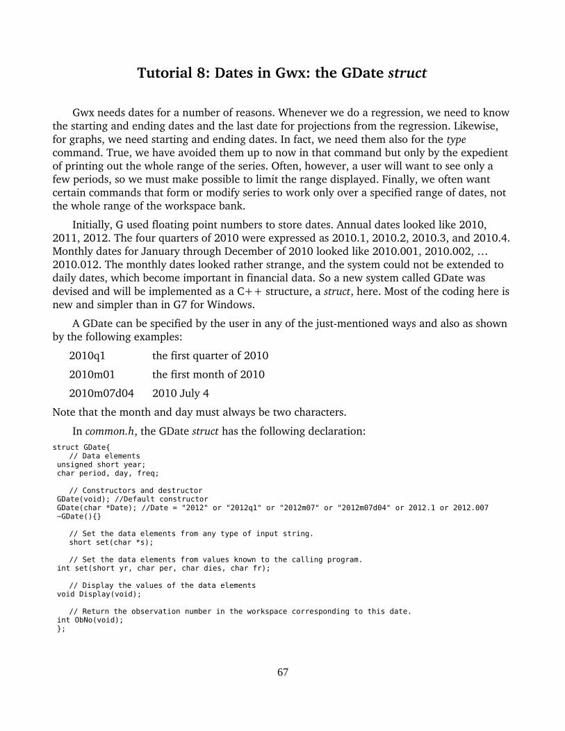
Tutorial 8: Dates in Gwx: the GDate struct
Gwx needs dates for a number of reasons. Whenever we do a regression, we need to know the starting and ending dates and the last date for projections from the regression. Likewise, for graphs, we need starting and ending dates. In fact, we need them also for the type command. True, we have avoided them up to now in that command but only by the expedient of printing out the whole range of the series. Often, however, a user will want to see only a few periods, so we must make possible to limit the range displayed. Finally, we often want certain commands that form or modify series to work only over a specified range of dates, not the whole range of the workspace bank.
Initially, G used floating point numbers to store dates. Annual dates looked like 2010, 2011, 2012. The four quarters of 2010 were expressed as 2010.1, 2010.2, 2010.3, and 2010.4.Monthly dates for January through December of 2010 looked like 2010.001, 2010.002, … 2010.012. The monthly dates looked rather strange, and the system could not be extended to daily dates, which become important in financial data. So a new system called GDate was devised and will be implemented as a C++ structure, a struct, here. Most of the coding here is new and simpler than in G7 for Windows.
A GDate can be specified by the user in any of the justmentioned ways and also as shown by the following examples:
2010q1 the first quarter of 2010
2010m01 the first month of 2010
2010m07d04 2010 July 4
Note that the month and day must always be two characters.
In common.h, the GDate struct has the following declaration:struct GDate{
// Data elements unsigned short year; char period, day, freq;
// Constructors and destructor GDate(void); //Default constructor GDate(char *Date); //Date = "2012" or "2012q1" or "2012m07" or "2012m07d04" or 2012.1 or 2012.007 ~GDate(){}
// Set the data elements from any type of input string.short set(char *s);
// Set the data elements from values known to the calling program. int set(short yr, char per, char dies, char fr);
// Display the values of the data elements void Display(void);
// Return the observation number in the workspace corresponding to this date. int ObNo(void); };
67
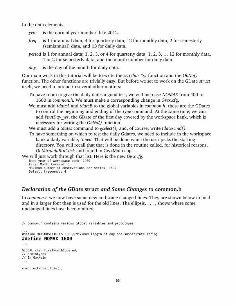
In the data elements,
year is the normal year number, like 2012.
freq is 1 for annual data, 4 for quarterly data, 12 for monthly data, 2 for semesterly (semiannual) data, and 13 for daily data.
period is 1 for annual data; 1, 2, 3, or 4 for quarterly data; 1, 2, 3, … 12 for monthly data,1 or 2 for semesterly data, and the month number for daily data.
day is the day of the month for daily data.
Our main work in this tutorial will be to write the set(char *s) function and the ObNo() function. The other functions are trivially easy. But before we set to work on the GDate struct itself, we need to attend to several other matters:
To have room to give the daily dates a good test, we will increase NOMAX from 400 to 1600 in common.h. We must make a corresponding change in Gwx.cfg.
We must add tdateA and tdateB to the global variables in common.h; these are the GDates to control the beginning and ending of the type command. At the same time, we can add FirstDay_ws, the GDate of the first day covered by the workspace bank, which is necessary for writing the ObNo() function.
We must add a tdates command to gselect(); and, of course, write tdatescmd(). To have something on which to test the daily Gdates, we need to include in the workspace
bank a daily variable, timed. That will be done when the user picks the starting directory. You will recall that that is done in the routine called, for historical reasons, OnMirandaBtnClick and found in GwxMain.cpp.
We will just work through that list. Here is the new Gwx.cfg:Base year of workspace bank; 1970First Month Covered; 1Maximum number of observations per series; 1600Default frequency; 4
Declaration of the GDate struct and Some Changes to common.h
In common.h we now have some new and some changed lines. They are shown below in bold and in a larger font than is used for the old lines. The ellipsis, . . . , shows where some unchanged lines have been omitted.
// common.h contains various global variables and prototypes
...#define MAXSUBSTITUTES 100 //Maximum length of any one susbstitute string
#define NOMAX 1600...
GLOBAL char FirstMonthCovered;// prototypes// In GwxMain...
void textsubstitute();
68
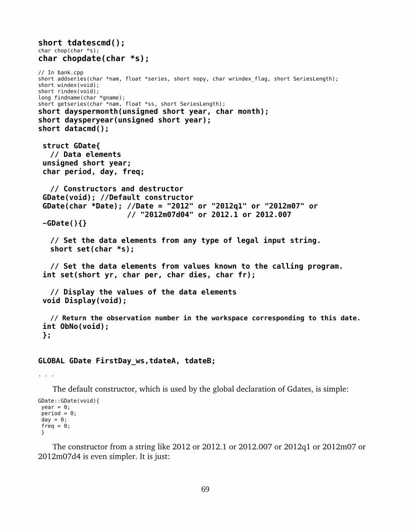
short tdatescmd();char chop(char *s);
char chopdate(char *s);
// In bank.cppshort addseries(char *nam, float *series, short nopy, char wrindex_flag, short SeriesLength);short windex(void);short rindex(void);long findname(char *gname);short getseries(char *nam, float *ss, short SeriesLength);
short dayspermonth(unsigned short year, char month);short daysperyear(unsigned short year);short datacmd(); struct GDate{
// Data elements unsigned short year; char period, day, freq;
// Constructors and destructor GDate(void); //Default constructor GDate(char *Date); //Date = "2012" or "2012q1" or "2012m07" or
// "2012m07d04" or 2012.1 or 2012.007 ~GDate(){}
// Set the data elements from any type of legal input string.short set(char *s);
// Set the data elements from values known to the calling program. int set(short yr, char per, char dies, char fr);
// Display the values of the data elements void Display(void);
// Return the observation number in the workspace corresponding to this date. int ObNo(void); }; GLOBAL GDate FirstDay_ws,tdateA, tdateB;
. . .
The default constructor, which is used by the global declaration of Gdates, is simple:GDate::GDate(void){ year = 0; period = 0; day = 0; freq = 0; }
The constructor from a string like 2012 or 2012.1 or 2012.007 or 2012q1 or 2012m07 or 2012m07d4 is even simpler. It is just:
69
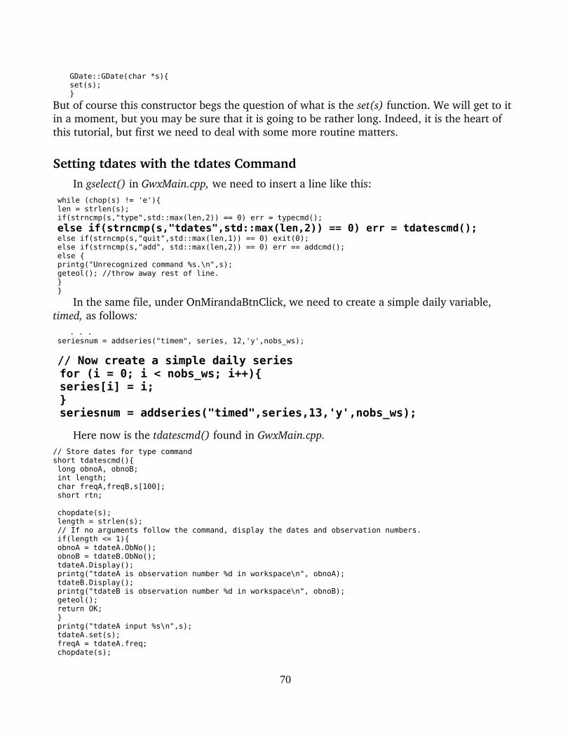
GDate::GDate(char *s){ set(s); }
But of course this constructor begs the question of what is the set(s) function. We will get to it in a moment, but you may be sure that it is going to be rather long. Indeed, it is the heart of this tutorial, but first we need to deal with some more routine matters.
Setting tdates with the tdates CommandIn gselect() in GwxMain.cpp, we need to insert a line like this:
while (chop(s) != 'e'){ len = strlen(s); if(strncmp(s,"type",std::max(len,2)) == 0) err = typecmd();
else if(strncmp(s,"tdates",std::max(len,2)) == 0) err = tdatescmd(); else if(strncmp(s,"quit",std::max(len,1)) == 0) exit(0); else if(strncmp(s,"add", std::max(len,2)) == 0) err == addcmd(); else { printg("Unrecognized command %s.\n",s); geteol(); //throw away rest of line. } }
In the same file, under OnMirandaBtnClick, we need to create a simple daily variable, timed, as follows:
. . . seriesnum = addseries("timem", series, 12,'y',nobs_ws);
// Now create a simple daily series for (i = 0; i < nobs_ws; i++){ series[i] = i; } seriesnum = addseries("timed",series,13,'y',nobs_ws);
Here now is the tdatescmd() found in GwxMain.cpp.// Store dates for type commandshort tdatescmd(){ long obnoA, obnoB; int length; char freqA,freqB,s[100]; short rtn;
chopdate(s); length = strlen(s); // If no arguments follow the command, display the dates and observation numbers. if(length <= 1){ obnoA = tdateA.ObNo(); obnoB = tdateB.ObNo(); tdateA.Display(); printg("tdateA is observation number %d in workspace\n", obnoA); tdateB.Display(); printg("tdateB is observation number %d in workspace\n", obnoB); geteol(); return OK; } printg("tdateA input %s\n",s); tdateA.set(s); freqA = tdateA.freq; chopdate(s);
70

printg("tdateB input %s\n",s); tdateB.set(s); freqB = tdateB.freq; tdateA.Display(); tdateB.Display(); if(tdateA.freq != tdateB.freq){ printg("Both tdates must have the same frequency. These two do not.\n"); return ERR; } //Check the observation numbers implied by these dates. obnoA = tdateA.ObNo(); obnoB = tdateB.ObNo();
if( obnoA < 0 || obnoA > nobs_ws) printg("Your tdateA is outside the range you set for the workspace. If you use it, Gwx will crash.\n"); if( obnoA > NOMAX) printg("Your tdateA is outside the range (0 to %d) Gwx is set to handle. If you use it, Gwx will crash.\n"), NOMAX; if( obnoB < 0 || obnoB > nobs_ws) printg("Your tdateB is outside the range you set for the workspace. If you use it, Gwx will crash.\n"); if( obnoB > NOMAX) printg("Your tdateB is outside the range (0 to %d) Gwx is set to handle. If you use it, Gwx will crash.\n", NOMAX);
return OK; }
The chopdate() FunctionThis routine uses several things we have not yet covered, first of all the chopdate()
function. If we try to read a date like 1970m01 with chop() , the date will be broken into two parts by the m. It will be easier to work with as all one string. One option was to add further complication to chop() to recognize a date string, as was done in G7. Another option was to require the user to always write something like y1970m01, so that the y would cause the stringto be read as all one alphabetical string. That seemed certain to irritate users. Another was to require the user to put all dates in quotes – with even more irritated users. It seemed simpler and clearer to have a version of chop() just for reading dates. Here it is, from GwxMain.cpp.
char chopdate(char *s){ short i; unsigned short cu; i = 0; char chopreturn = 'a';
while(i < MAXLINE){ cu = *pinbuf++; // Spaces or Tabs if(cu == ' ' || cu == '\t'){ // found a space or tab if(i== 0) continue; // eat up white space s[i] = '\0'; // end the word being returned return chopreturn; } // End of line if(cu == 0){ // found an end of line s[i] = '\0'; // end the word being built if(i > 0) { // if a word has been started pinbuf--; // back up one character so the EOL will be read next time return chopreturn; // return the word that had been started } else return 'e'; }
if(i==0 && cu == ';'){ chopreturn = ';';
71

return chopreturn; } if(i == 0 && (isalnum(cu))){ // found a letter or number chopreturn = 'a'; s[i++] = cu;
while(isalnum(*pinbuf) || *pinbuf == '.') { s[i++] = *pinbuf++; } s[i] = '\0'; return chopreturn; } } // Should not get here, but if we do s[MAXLINE-1] = '\0'; return ERR; }
There is little new here. The key line which keeps building the string as long as the characters are letters, digits, or the period chasracter, '.', has been put in bold and enlarged type. We havealso provided for the return of a semicolon, ';' , if it is found at the beginning of a chop. This ability will be used in writing the matdata command in the next tutorial.
Giving Values to a GDate, the set() FunctionsThe tdates command also used the set() function of the GDate. There are two versions of
set(). One is as simple as can be but is of limited usefulness:int GDate::set(short yr, char per, char dies, char fr){ year = yr; period = per; day = dies; freq = fr; return OK; }
The other version of set() takes as its argument a string of any of the types mentioned above. It is a long function but not complicated. It just trudges through the string figuring out what needs to be done and doing it. I have tried to comment it sufficiently to make it easy reading. //This constructor and set() function handle both dates like 2012 or 2012.1 or 2012.007 and// dates like "2012" or "2012q1" or "2012m07" or "2012m07d4".// The first, older form cannot handle daily dates.
GDate::GDate(char *s){ set(s); }short GDate::set(char *s){ short i,j; char room[5]; day = 0; // Get the year, which should be the first 4 digits in all formats i = 0; while (i < 4){ if(!isdigit(s[i])) goto error; room[i] = s[i++]; } room[4] = '\0'; year = atoi(room); // If s[4] = '\0', it is an annual date if(s[4]=='\0'){
72

freq = 1; period = 1; day = 0; return OK; }
// If s[4] is a '.', we have a date of the form 2000.1 or 2000.001. if(s[4] == '.'){ if(s[5] == '0'){ // a monthly date if(isdigit(s[6]) && isdigit(s[7])){ freq = 12; room[0] = s[6]; room[1] = s[7]; room[2] = '\0'; period = atoi(room); return OK; } else goto error; } // A quarterly or semiannual date if(isdigit(s[5])){ room[0] = s[5]; room[1] = '\0'; period = atoi(room); } else goto error;
if(period <= 4){ freq = 4; return OK; } else if(period <= 6){ freq = 2; period = period - 4; return OK; } else goto error; }
// It must be a date like "2012q1" or "2012m07" or "2012m07d4". // Is it a quarterly date? if(s[4] == 'q'){ freq = 4; if(isdigit(s[5])){ room[0] = s[5]; room[1] = '\0'; period = atoi(room); if(period < 1 || period > 4) goto error; return OK; } else goto error; } // Is it a semesterly date? if(s[4] == 's'){ freq = 2; if(isdigit(s[5])){ room[0] = s[5]; room[1] = '\0'; period = atoi(room); if(period < 1 || period > 2) goto error; return OK; } else goto error; } if(s[4]== 'm'){//monthly or daily date. freq = 12; if(isdigit(s[5]) && isdigit(s[6])){ room[0] = s[5];
73
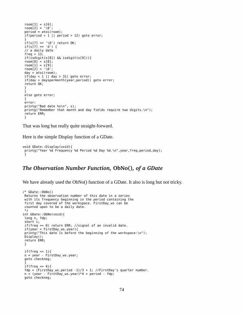
room[1] = s[6]; room[2] = '\0'; period = atoi(room); if(period < 1 || period > 12) goto error; } if(s[7] == '\0') return OK; if(s[7] == 'd') { // a daily date freq = 13; if(isdigit(s[8]) && isdigit(s[9])){ room[0] = s[8]; room[1] = s[9]; room[2] = '\0'; day = atoi(room); if(day < 1 || day > 31) goto error; if(day > dayspermonth(year,period)) goto error; return OK; } } else goto error; } error: printg("Bad date %s\n", s); printg("Remember that month and day fields require two digits.\n"); return ERR; }
That was long but really quite straight-forward.
Here is the simple Display function of a GDate. void GDate::Display(void){ printg("Year %d Frequency %d Period %d Day %d.\n",year,freq,period,day); }
The Observation Number Function, ObNo(), of a GDate
We have already used the ObNo() function of a GDate. It also is long but not tricky.
/* GDate::ObNo() Returns the observation number of this date in a series with its frequency beginning in the period containing the first day covered of the workspace. FirstDay_ws can be counted upon to be a daily date. */int GDate::ObNo(void){ long n, fdp; short i; if(freq == 0) return ERR; //signal of an invalid date. if(year < FirstDay_ws.year){ printg("This date is before the beginning of the workspace:\n"); Display(); return ERR; }
if(freq == 1){ n = year - FirstDay_ws.year; goto checkneg; } if(freq == 4){ fdp = (FirstDay_ws.period -1)/3 + 1; //FirstDay's quarter number. n = (year - FirstDay_ws.year)*4 + period - fdp; goto checkneg;
74
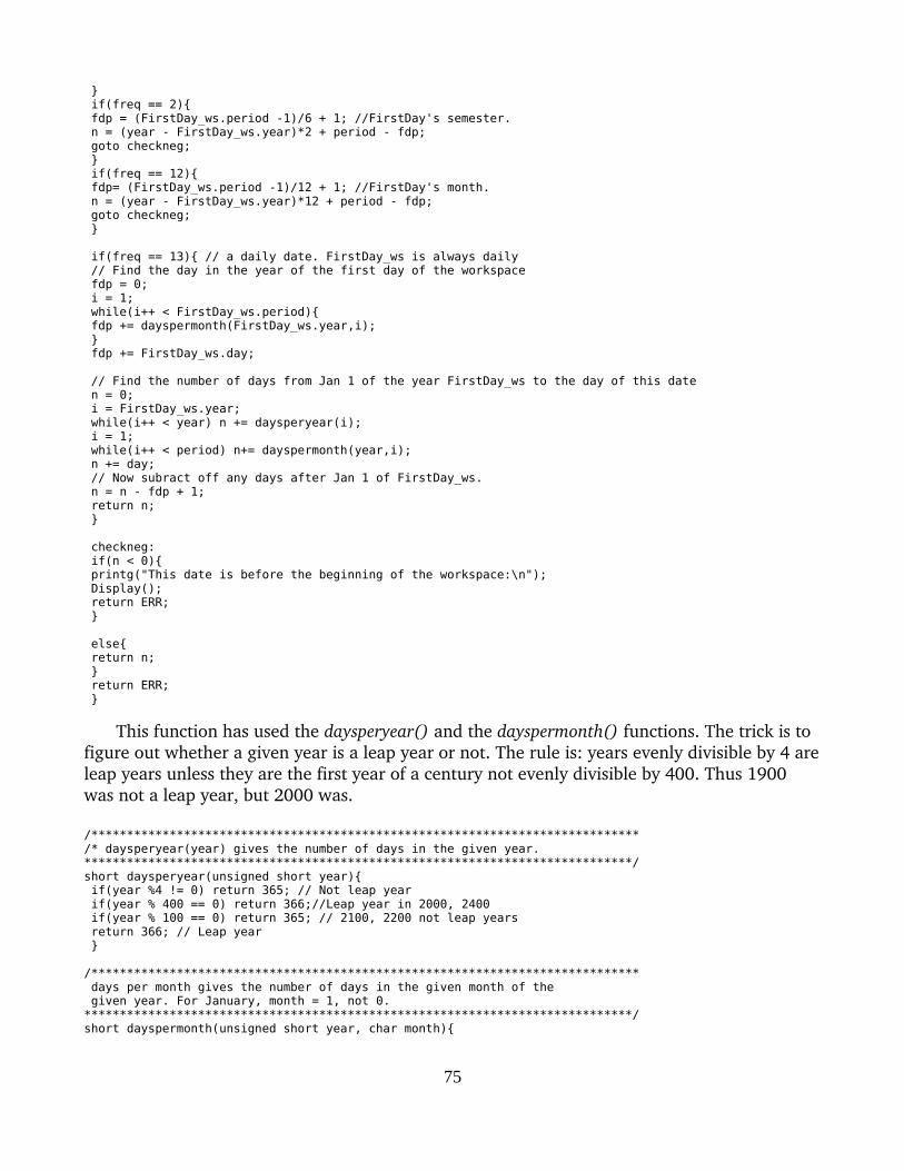
} if(freq == 2){ fdp = (FirstDay_ws.period -1)/6 + 1; //FirstDay's semester. n = (year - FirstDay_ws.year)*2 + period - fdp; goto checkneg; } if(freq == 12){ fdp= (FirstDay_ws.period -1)/12 + 1; //FirstDay's month. n = (year - FirstDay_ws.year)*12 + period - fdp; goto checkneg; }
if(freq == 13){ // a daily date. FirstDay_ws is always daily // Find the day in the year of the first day of the workspace fdp = 0; i = 1; while(i++ < FirstDay_ws.period){ fdp += dayspermonth(FirstDay_ws.year,i); } fdp += FirstDay_ws.day;
// Find the number of days from Jan 1 of the year FirstDay_ws to the day of this date n = 0; i = FirstDay_ws.year; while(i++ < year) n += daysperyear(i); i = 1; while(i++ < period) n+= dayspermonth(year,i); n += day; // Now subract off any days after Jan 1 of FirstDay_ws. n = n - fdp + 1; return n; }
checkneg: if(n < 0){ printg("This date is before the beginning of the workspace:\n"); Display(); return ERR; }
else{ return n; } return ERR; }
This function has used the daysperyear() and the dayspermonth() functions. The trick is to figure out whether a given year is a leap year or not. The rule is: years evenly divisible by 4 areleap years unless they are the first year of a century not evenly divisible by 400. Thus 1900 was not a leap year, but 2000 was.
/*****************************************************************************/* daysperyear(year) gives the number of days in the given year.*****************************************************************************/short daysperyear(unsigned short year){ if(year %4 != 0) return 365; // Not leap year if(year % 400 == 0) return 366;//Leap year in 2000, 2400 if(year % 100 == 0) return 365; // 2100, 2200 not leap years return 366; // Leap year }
/***************************************************************************** days per month gives the number of days in the given month of the given year. For January, month = 1, not 0.*****************************************************************************/short dayspermonth(unsigned short year, char month){
75

char DaysInMonth[] = {31,28,31,30,31,30,31,31,30,31,30,31}; if(month < 1 || month >12){ printf("Invalid month %d.\n", month); return -1; } if(month != 2) return DaysInMonth[month-1]; if (daysperyear(year)== 365) return 28; //not leap year return 29; //leap year }
The type Command with tdates.That finishes up the GDate struct. Now we turn to the final matter of this tutorial,
rewriting the type command to use tdateA and tdateB, which were set by user's giving a tdate command. Here is the typecmd() command, which is in GwxMain.cpp.short typecmd(){ char s[100]; short npy,i,j,secondline; unsigned short obnoA,obnoB; float series[NOMAX]; short year, month, limit;
chop(s); npy = getseries(s,series,-1); if(npy == -1){ printg("%s was not found.\n",s); return -1; } if(tdateA.freq != tdateB.freq){ printg("Frequencies of the two tdates are not the same.\n"); return ERR; } if(npy != tdateA.freq){ printg("Frequency of %s, %d, does not match that of tdates, %d\n.",s,npy,tdateA.freq); return ERR; } printg("Here is %s:\n", s); obnoA = tdateA.ObNo(); obnoB = tdateB.ObNo(); if(npy == 4){//quarterly data for(i = obnoA; i <= obnoB; i = i+4){ printg("%dq%d ", jahrba+(i/4), tdateA.period); // print the year and first quarter shown for(j=0;j<4;j++) // print the four quarterly values if(i+j <= obnoB)printg(" %12.3f", series[i+j]); printg("\n"); // print the new line } } else if(npy == 12){//monthly data secondline = (tdateA.period+6) % 12;
for(i = obnoA; i <= obnoB; i = i+12){ printg("%dm%d ",jahrba+(i/12), tdateA.period); // print the year and first month shown for(j=0;j<6;j++) // print the values for January - June if(i+j <= obnoB) printg(" %12.4f", series[i+j]); printg("\n"); // print the new line
printg("%dm%d ",jahrba+(i/12), secondline); // print the year and first month shown for(j=6;j<12;j++) // print the values for January - June if(i+j <= obnoB) printg(" %12.4f", series[i+j]); printg("\n"); // print the new line } } else if (npy == 13){ // daily data // Adjust obnoA to be first day of the month of tdateA. // This will leave obnoA positive because FirstDay_ws is always the first day of a month.
76
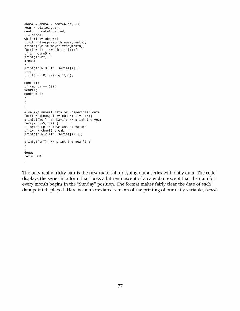
obnoA = obnoA - tdateA.day +1; year = tdateA.year; month = tdateA.period; i = obnoA; while(i <= obnoB){ limit = dayspermonth(year,month); printg("\n %d %d\n",year,month); for(j = 1; j <= limit; j++){ if(i > obnoB){ printg("\n"); break; } printg(" %10.3f", series[i]); i++; if(j%7 == 0) printg("\n"); } month++; if (month == 13){ year++; month = 1; } } }
else {// annual data or unspecified data for(i = obnoA; i <= obnoB; i = i+5){ printg("%d ",jahrba+i); // print the year for(j=0;j<5;j++) { // print up to five annual values if(i+j > obnoB) break; printg(" %12.4f", series[i+j]); } printg("\n"); // print the new line } } done: return OK; }
The only really tricky part is the new material for typing out a series with daily data. The code displays the series in a form that looks a bit reminiscent of a calendar, except that the data for every month begins in the “Sunday” position. The format makes fairly clear the date of each data point displayed. Here is an abbreviated version of the printing of our daily variable, timed.
77

1971 1 366.000 367.000 368.000 369.000 370.000 371.000 372.000 373.000 374.000 375.000 376.000 377.000 378.000 379.000 380.000 381.000 382.000 383.000 384.000 385.000 386.000 387.000 388.000 389.000 390.000 391.000 392.000 393.000 394.000 395.000 396.000 1971 2 397.000 398.000 399.000 400.000 401.000 402.000 403.000 404.000 405.000 406.000 407.000 408.000 409.000 410.000 411.000 412.000 413.000 414.000 415.000 416.000 417.000 418.000 419.000 420.000 421.000 422.000 423.000 424.000
1971 3 425.000 426.000 427.000 428.000 429.000 430.000 431.000 432.000 433.000 434.000 435.000 436.000 437.000 438.000 439.000 440.000 441.000 442.000 443.000 444.000 445.000 446.000 447.000 448.000 449.000 450.000 451.000 452.000 453.000 454.000 455.000 . . . 1972 1 731.000 732.000 733.000 734.000 735.000 736.000 737.000 738.000 739.000 740.000 741.000 742.000 743.000 744.000 745.000 746.000 747.000 748.000 749.000 750.000 751.000 752.000 753.000 754.000 755.000 756.000 757.000 758.000 759.000 760.000 761.000 1972 2 762.000 763.000 764.000 765.000 766.000 767.000 768.000 769.000 770.000 771.000 772.000 773.000 774.000 775.000 776.000 777.000 778.000 779.000 780.000 781.000 782.000 783.000 784.000 785.000 786.000 787.000 788.000 789.000 790.000 1972 3 791.000 792.000 793.000 794.000 795.000 796.000 797.000 798.000 799.000 800.000 801.000 802.000 803.000 804.000 805.000 806.000 807.000 808.000 809.000 810.000 811.000 812.000 813.000 814.000 815.000 816.000 817.000 818.000 819.000 820.000 821.000
Note that the program figured out correctly that 1972 was a leap year but that 1971 was not.
Test It Out!It is easy to test the new code. Use the tdate command to set up dates and type out the
variables we have created with them. You can also try making some mistakes, and see if you get caught! You might try:
tdates 1971 2000type timeatdates 1971m01d01 1974m012 tdatestype timedtype timea
The last command is a mistake on the part of the user.
78

Tutorial 9: The data and matdata CommandsOur device of putting some series into the workspace when it is created has served us well
to allow us to test all of our programming up to this point. But now we need to write a command to introduce data from an ASCII file into the workspace. We will start off with some rather artificial data that makes it easy to check the functioning of the program. But once that works, we can use the same command to introduce real data like U.S. Gross domestic product. We will call the command just data. We can illustrate it with a file, which we can call mydata.dat, which looks like this:
data integers 19700 1 2 3 4 5 6 7 8 910 11 12 13 14 15 16 17 18 1920 21 22;
We want to be able to give Gwx a command like this:
add mydata.datand have it read the file and introduce a series called integers into the workspace, so that thesethree commands
add integers.dattdates 1970 2000type integers
will result in the following display in the Results window:
Here is integers: 1970 0.0000 1.0000 2.0000 3.0000 4.0000 1975 5.0000 6.0000 7.0000 8.0000 9.0000 1980 10.0000 11.0000 12.0000 13.0000 14.0000 1985 15.0000 16.0000 17.0000 18.0000 19.0000 1990 20.0000 21.0000 22.0000 -0.0000 -0.0000 1995 -0.0000 -0.0000 -0.0000 -0.0000 -0.0000 2000 -0.0000
Once we we can introduce this rather silly data, we can introduce any data. The following tutorials will then create many commands for working with data.
We are going to assume that the data command and the data following it are in a file which will be “added” to the runstream. In other words, we will assume that the user does not give the data command directly in the command box; it will always be in a file that is introduced by an add command. This assumption is not very restrictive. It would be a foolish user who typed in data directly to the command box with no external record of what was typed.
First Version; Date on Command LineLet me say at the outset that in this first version we will concentrate on the logic of the
79
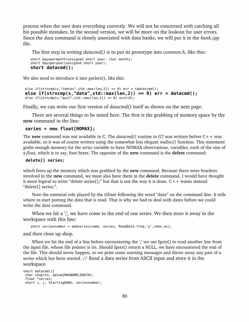
process when the user does everything correctly. We will not be concerned with catching all his possible mistakes. In the second version, we will be more on the lookout for user errors. Since the data command is closely associated with data banks, we will put it in the bank.cpp file.
The first step in writing datacmd() is to put its prototype into common.h, like this: short dayspermonth(unsigned short year, char month);short daysperyear(unsigned short year);
short datacmd();
We also need to introduce it into gselect(), like this:
else if(strncmp(s,"tdates",std::max(len,2)) == 0) err = tdatescmd();
else if(strncmp(s,"data",std::max(len,2)) == 0) err = datacmd(); else if(strncmp(s,"quit",std::max(len,1)) == 0) exit(0);
Finally, we can write our first version of datacmd() itself as shown on the next page.
There are several things to be noted here. The first is the grabbing of memory space by thenew command in the line:
series = new float[NOMAX];
The new command was not available in C. The datacmd() routine in G7 was written before C++ was available, so it was of course written using the somewhat less elegant malloc() function. This statement grabs enough memory for the series variable to have NOMAX observations, variables, each of the size ofa float, which is to say, four bytes. The opposite of the new command is the delete command:
delete[] series;
which frees up the memory which was grabbed by the new command. Because there were brackets involved in the new command, we must also have them in the delete command. I would have thought it more logical to write “delete series[];” but that is not the way it is done. C++ wants instead “delete[] series;”.
Note the essential role played by the GDate following the word “data” on the command line. It tellswhere to start putting the data that is read. That is why we had to deal with dates before we could write the data command.
When we hit a ';', we have come to the end of one series. We then store it away in the workspace with this line:
short seriesnumber = addseries(name, series, ReadDate.freq,'y',nobs_ws);
and then close up shop.
When we hit the end of a line before encountering the ';' we use fgets() to read another line from the input file, whose file pointer is iin. Should fgets() return a NULL, we have encountered the end of the file. This should never happen, so we print some warning messages and throw away any part of a series which has been started. // Read a data series from ASCII input and store it in the workspaceshort datacmd(){ char choprtn, datum[MAXNAMELENGTH]; float *series; short i, j, StartingObNo, seriesnumber;
80

char name[MAXNAMELENGTH], rdate[12]; GDate ReadDate;
series = new float[NOMAX];
// Get the name of the variable to be put into the workspace if((chop(name)) != 'a'){ printg("Error: the variable's name in a data command must begin with a letter.\n"); return ERR; } // Initialize series to MISSING; for(i =0; i < NOMAX; i++) series[i] = MISSING;
// Read the date of the first observation to be read. chopdate(rdate); ReadDate.set(rdate); StartingObNo = ReadDate.ObNo(); i = StartingObNo;
// Read the data numbers until we hit a ';'. Store the data in the series array. while(i < NOMAX){
choprtn = chop(datum); if(choprtn == 'n'){ series[i++] = atof(datum); // Convert an ASCII string to a floating point number. } else if(choprtn == ';'){ // End of data for this series short seriesnumber = addseries(name, series, ReadDate.freq,'y',nobs_ws); goto closeup; } else if(choprtn == 'e'){ // End of line; get next line from the input file.
if(fgets(inbufAsRead,MAXLINE,iin) != NULL){printg(inbufAsRead);
j = 0; // Remove the '\n' at the end of inbufAsRead for comparability
// with what comes from CmdBox. while(inbufAsRead[j] != '\n') j++; inbufAsRead[j] = '\0'; // Perform text substitution textsubstitute(); pinbuf = inbuf; }
else { // We have hit the end of the input file. printg("You encountered an End of File while reading data. \n"); printg("Did you forget a semicolon at the end of a series?\n"); seriesnumber = ERR; goto closeup; } } }
closeup: delete[] series; return seriesnumber; }
81
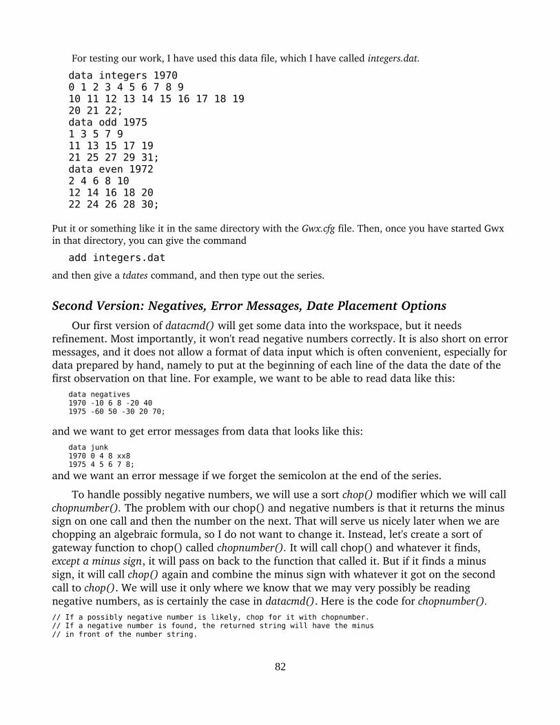
For testing our work, I have used this data file, which I have called integers.dat.
data integers 19700 1 2 3 4 5 6 7 8 910 11 12 13 14 15 16 17 18 1920 21 22;data odd 19751 3 5 7 911 13 15 17 1921 25 27 29 31;data even 19722 4 6 8 1012 14 16 18 2022 24 26 28 30;
Put it or something like it in the same directory with the Gwx.cfg file. Then, once you have started Gwx in that directory, you can give the command
add integers.dat
and then give a tdates command, and then type out the series.
Second Version: Negatives, Error Messages, Date Placement OptionsOur first version of datacmd() will get some data into the workspace, but it needs
refinement. Most importantly, it won't read negative numbers correctly. It is also short on errormessages, and it does not allow a format of data input which is often convenient, especially fordata prepared by hand, namely to put at the beginning of each line of the data the date of the first observation on that line. For example, we want to be able to read data like this:
data negatives1970 -10 6 8 -20 40 1975 -60 50 -30 20 70;
and we want to get error messages from data that looks like this:data junk1970 0 4 8 xx81975 4 5 6 7 8;
and we want an error message if we forget the semicolon at the end of the series.
To handle possibly negative numbers, we will use a sort chop() modifier which we will callchopnumber(). The problem with our chop() and negative numbers is that it returns the minus sign on one call and then the number on the next. That will serve us nicely later when we are chopping an algebraic formula, so I do not want to change it. Instead, let's create a sort of gateway function to chop() called chopnumber(). It will call chop() and whatever it finds, except a minus sign, it will pass on back to the function that called it. But if it finds a minus sign, it will call chop() again and combine the minus sign with whatever it got on the second call to chop(). We will use it only where we know that we may very possibly be reading negative numbers, as is certainly the case in datacmd(). Here is the code for chopnumber(). // If a possibly negative number is likely, chop for it with chopnumber.// If a negative number is found, the returned string will have the minus// in front of the number string.
82
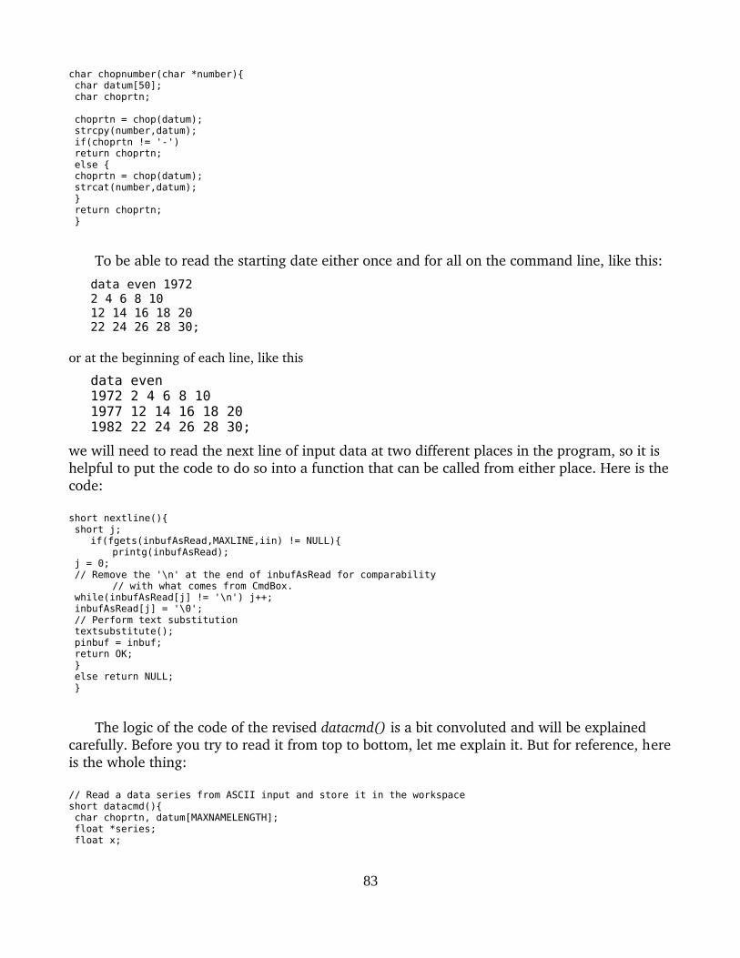
char chopnumber(char *number){ char datum[50]; char choprtn;
choprtn = chop(datum); strcpy(number,datum); if(choprtn != '-') return choprtn; else { choprtn = chop(datum); strcat(number,datum); } return choprtn; }
To be able to read the starting date either once and for all on the command line, like this:
data even 19722 4 6 8 1012 14 16 18 2022 24 26 28 30;
or at the beginning of each line, like this
data even1972 2 4 6 8 101977 12 14 16 18 201982 22 24 26 28 30;
we will need to read the next line of input data at two different places in the program, so it is helpful to put the code to do so into a function that can be called from either place. Here is thecode:
short nextline(){ short j;
if(fgets(inbufAsRead,MAXLINE,iin) != NULL){printg(inbufAsRead);
j = 0; // Remove the '\n' at the end of inbufAsRead for comparability
// with what comes from CmdBox. while(inbufAsRead[j] != '\n') j++; inbufAsRead[j] = '\0'; // Perform text substitution textsubstitute(); pinbuf = inbuf; return OK; } else return NULL; }
The logic of the code of the revised datacmd() is a bit convoluted and will be explained carefully. Before you try to read it from top to bottom, let me explain it. But for reference, hereis the whole thing:
// Read a data series from ASCII input and store it in the workspaceshort datacmd(){ char choprtn, datum[MAXNAMELENGTH]; float *series; float x;
83

short i, j, StartingObNo, seriesnumber, datereturn; char name[MAXNAMELENGTH], rdate[12]; bool DateOnCommandLine; GDate ReadDate; series = new float[NOMAX];
// Get the name of the variable to be put into the workspace if((chop(name)) != 'a'){ printg("Error: the variable's name in a data command must begin with a letter.\n"); return ERR; } // Initialize series to MISSING; for(i =0; i < NOMAX; i++) series[i] = MISSING;
// Read the date of the first observation to be read. DateOnCommandLine = false; choprtn = chopdate(rdate); if (choprtn == 'a'){ DateOnCommandLine = true; ReadDate.set(rdate); } if(DateOnCommandLine == false){ nextline(); choprtn = chopdate(rdate); ReadDate.set(rdate); } StartingObNo = ReadDate.ObNo(); i = StartingObNo;
while(i < NOMAX){ // Start the big while loop. choprtn = chopnumber(datum); if(choprtn == 'n'){ series[i++] = atof(datum); // Convert ASCII string to floating point number } else if(choprtn == ';'){ // End of data for this series short seriesnumber = addseries(name, series, ReadDate.freq,'y',nobs_ws); goto closeup; } else if(choprtn == 'e'){ // End of line; get next line from the input file. if(nextline() == NULL){ // We have hit the end of the input file. printg("You encountered an End of File while reading data. \n"); printg("Did you forget a semicolon at the end of a series?\n"); seriesnumber = ERR; goto closeup; } // If the date is on each line, read it for the line just read // and reset i. else if (DateOnCommandLine == false){ choprtn = chopdate(rdate); datereturn = ReadDate.set(rdate); if (datereturn == ERR){ printg("There is a problem in your data input.\n"); printg("I am guessing you forgot a semicolon at the end.\n"); pinbuf = inbuf; seriesnumber = addseries(name, series, ReadDate.freq,'y',nobs_ws); goto closeup; } StartingObNo = ReadDate.ObNo(); i = StartingObNo; } } else goto junkonline;
} // End of big while loop
closeup: delete[] series; return seriesnumber;
84

junkonline: printg("Junk on this line:\n"); printg("%s\n",inbufAsRead); seriesnumber = ERR; goto closeup; }
After getting the name of the variable and clearing the series array to MISSING, we figure out whether or not the beginning date is on the command line or whether each line will have its own beginning date. We use a boolian (true or false) variable, DateOnCommandLine, to record what we find. We first set it to false, then do a chopdate() call. If we find a date, we change DateOnCommandLine to true and set the GDate ReadDate to value that was found. If we did not find a date on the command line, we call nextline() and then read the starting date from the first line of data. Either way, we end up with the starting date in ReadDate, and we get its observation number. Here is that opening code:
// Read the date of the first observation to be read. DateOnCommandLine = false; choprtn = chopdate(rdate); if (choprtn == 'a'){ DateOnCommandLine = true; ReadDate.set(rdate); }
// If the date is at the beginning of the line, read it:if(DateOnCommandLine == false){
nextline(); choprtn = chopdate(rdate); ReadDate.set(rdate); }
StartingObNo = ReadDate.ObNo(); i = StartingObNo;
We then set up a big while loop on i, the observation number. This is a somewhat unusual while loop in that the index i is changed not only by simple incrementing but also possibly by reading dates from the beginning of each line.
As we start to work inside the while loop, we know that the starting date on the line, if any, has already been read. So we can go right to work as follows: choprtn = chopnumber(datum); if(choprtn == 'n'){ series[i++] = atof(datum); // Convert ASCII string to floating point number } else if(choprtn == ';'){ // End of data for this series short seriesnumber = addseries(name, series, ReadDate.freq,'y',nobs_ws); goto closeup; }
If a semicolon is encountered, the reading of the series is stopped, and the series is put into theworkspace bank.
If an endofline is encountered, the next line is brought into inbuf. If we are in the dateoneveryline mode, we read the date and reset i to the observation number of the date it specifies. If, on that read, a bad data is encountered, the program guesses that the user forgot
85

the semicolon at the end of the series and has gone on to the next command in the add file. It prints an error message but also stores the series it has read into the bank, just as if there had been a semicolon. Then it backs up the pointer to the input buffer to the beginning and returnsto let gselect() deal with the problem, if one remains. Here is that code: if (datereturn == ERR){ printg("There is a problem in your data input.\n"); printg("I am guessing you forgot a semicolon at the end.\n"); pinbuf = inbuf; seriesnumber = addseries(name, series, ReadDate.freq,'y',nobs_ws); goto closeup; }
If bad data is encountered anywhere, we go to the junkonline label and display the faulty line. If other data lines follow the one with the junk, they will be displayed with the “unrecognized command” message.
Now it should be possible to make sense of the program with a toptobottom reading of it.
Here is a file, integers.dat, that I used in testing:data integers 19700 1 2 3 4 5 6 7 8 910 11 12 13 14 15 16 17 18 1920 21 22;data odd 19751 3 5 7 911 13 15 17 1921 25 27 29 31;data even 19722 4 6 8 1012 14 16 18 2022 24 26 28 30;
data threes1970 3 6 9 12 151975 18 21 24 27 301980 33 36 39 42 45;data fours1970 0 4 8 xx81975 4 5 6 7 8data negatives1970 -10 6 8 -20;
data nosemicolon1970 0 4 8 81975 4 5 6 7 8
data right1970 0 4 8 121975 4 5 6 7 8;
tdates 1970 1990
86
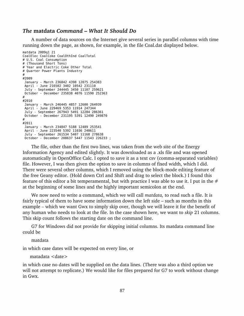
The matdata Command – What It Should Do A number of data sources on the Internet give several series in parallel columns with time
running down the page, as shown, for example, in the file Coal.dat displayed below. matdata 2009q1 21 CoalElec CoalCoke CoalOthInd CoalTotal # U.S. Coal Consumption # (Thousand Short Tons) # Year and Electric Coke Other Total # Quarter Power Plants Industry# #2009 January - March 236842 4398 12075 254383 April - June 216502 3402 10542 231110 July - September 244445 3450 11107 259621 October - December 235838 4076 11590 252363# #2010 January - March 246445 4857 12600 264939 April - June 229469 5353 11914 247344 July - September 267943 5491 12284 286361 October - December 231195 5391 12490 249870# #2011 January - March 234847 5188 12489 253541 April - June 223540 5392 11036 240611 July - September 261534 5407 11168 278638 October - December 208637 5447 11543 226233 ;
The file, other than the first two lines, was taken from the web site of the Energy Information Agency and edited slightly. It was downloaded as a .xls file and was opened automatically in OpenOffice Calc. I opted to save it as a text csv (commaseparated variables) file. However, I was then given the option to save in columns of fixed width, which I did. There were several other columns, which I removed using the blockmode editing feature of the free Geany editor. (Hold down Ctrl and Shift and drag to select the block.) I found this feature of this editor a bit temperamental, but with practice I was able to use it. I put in the # at the beginning of some lines and the highly important semicolon at the end.
We now need to write a command, which we will call matdata, to read such a file. It is fairly typical of them to have some information down the left side – such as months in this example – which we want Gwx to simply skip over, though we will leave it for the benefit of any human who needs to look at the file. In the case shown here, we want to skip 21 columns. This skip count follows the starting date on the command line.
G7 for Windows did not provide for skipping initial columns. Its matdata command line could be
matdata
in which case dates will be expected on every line, or
matadata <date>
in which case no dates will be supplied on the data lines. (There was also a third option we will not attempt to replicate.) We would like for files prepared for G7 to work without change in Gwx.
87
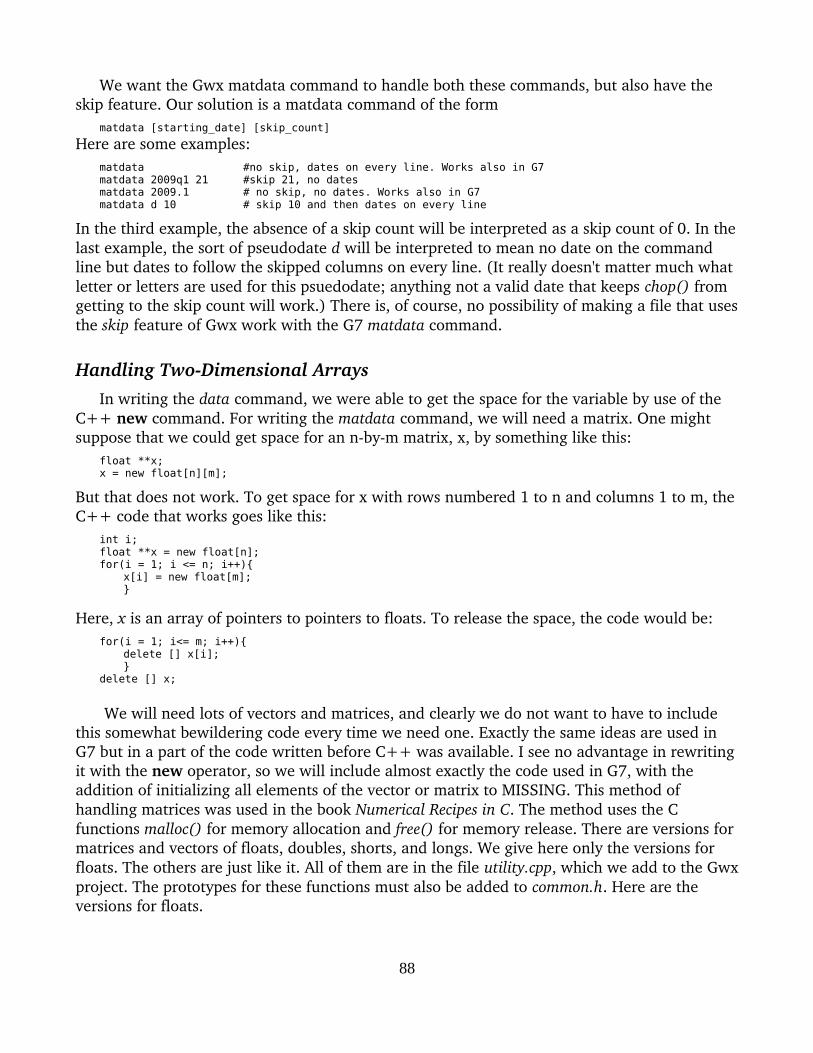
We want the Gwx matdata command to handle both these commands, but also have the skip feature. Our solution is a matdata command of the form
matdata [starting_date] [skip_count]
Here are some examples:matdata #no skip, dates on every line. Works also in G7matdata 2009q1 21 #skip 21, no datesmatdata 2009.1 # no skip, no dates. Works also in G7matdata d 10 # skip 10 and then dates on every line
In the third example, the absence of a skip count will be interpreted as a skip count of 0. In thelast example, the sort of pseudodate d will be interpreted to mean no date on the command line but dates to follow the skipped columns on every line. (It really doesn't matter much what letter or letters are used for this psuedodate; anything not a valid date that keeps chop() from getting to the skip count will work.) There is, of course, no possibility of making a file that usesthe skip feature of Gwx work with the G7 matdata command.
Handling TwoDimensional ArraysIn writing the data command, we were able to get the space for the variable by use of the
C++ new command. For writing the matdata command, we will need a matrix. One might suppose that we could get space for an nbym matrix, x, by something like this:
float **x; x = new float[n][m];
But that does not work. To get space for x with rows numbered 1 to n and columns 1 to m, theC++ code that works goes like this:
int i;float **x = new float[n];for(i = 1; i <= n; i++){
x[i] = new float[m];}
Here, x is an array of pointers to pointers to floats. To release the space, the code would be:for(i = 1; i<= m; i++){
delete [] x[i];}
delete [] x;
We will need lots of vectors and matrices, and clearly we do not want to have to include this somewhat bewildering code every time we need one. Exactly the same ideas are used in G7 but in a part of the code written before C++ was available. I see no advantage in rewritingit with the new operator, so we will include almost exactly the code used in G7, with the addition of initializing all elements of the vector or matrix to MISSING. This method of handling matrices was used in the book Numerical Recipes in C. The method uses the C functions malloc() for memory allocation and free() for memory release. There are versions for matrices and vectors of floats, doubles, shorts, and longs. We give here only the versions for floats. The others are just like it. All of them are in the file utility.cpp, which we add to the Gwxproject. The prototypes for these functions must also be added to common.h. Here are the versions for floats.
88

float *vector(int nl, int nh){float *v;
int i, top; top = nh - nl + 1;
v=(float *)malloc((unsigned) top*sizeof(float));if (!v){
printg(msguti1);return 0;}
for (i = 0; i < top; i++) v[i] = MISSING;
return v-nl;}
float **matrix(int nrl, int nrh, int ncl, int nch){ int i,j,k; float **m; int toprow = nrh-nrl+1; int topcol = nch-ncl+1;
m=(float **) malloc((unsigned) toprow*sizeof(float*)); if (!m){ printg(msguti1); return 0; } m -= nrl; for(i = nrl; i <= nrh; i++) m[i] = 0;
for(i=nrl;i<=nrh;i++){ m[i]=(float *) malloc((unsigned) topcol*sizeof(float)); if (!m[i]){ printg(msguti1); for(k = nrl; k < i; k++){ free((void *)(m[i]+ncl)); } free((void *)(m+nrl)); return(0); } m[i] -= ncl; } for (i = nrl; i <= nrh; i++){ for(j = ncl; j <= nch; j++){ m[i][j] = MISSING; } } return m; }
void free_vector(float *v, int nl){ if(v != 0) free((char*) (v+nl)); }
void free_matrix(float **m, int nrl, int nrh, int ncl){ int i;
if(m == 0) return; for(i=nrh;i>=nrl;i--){ if(m[i]+ncl) free( (m[i]+ncl) ); } free((void*) (m+nrl)); }
89
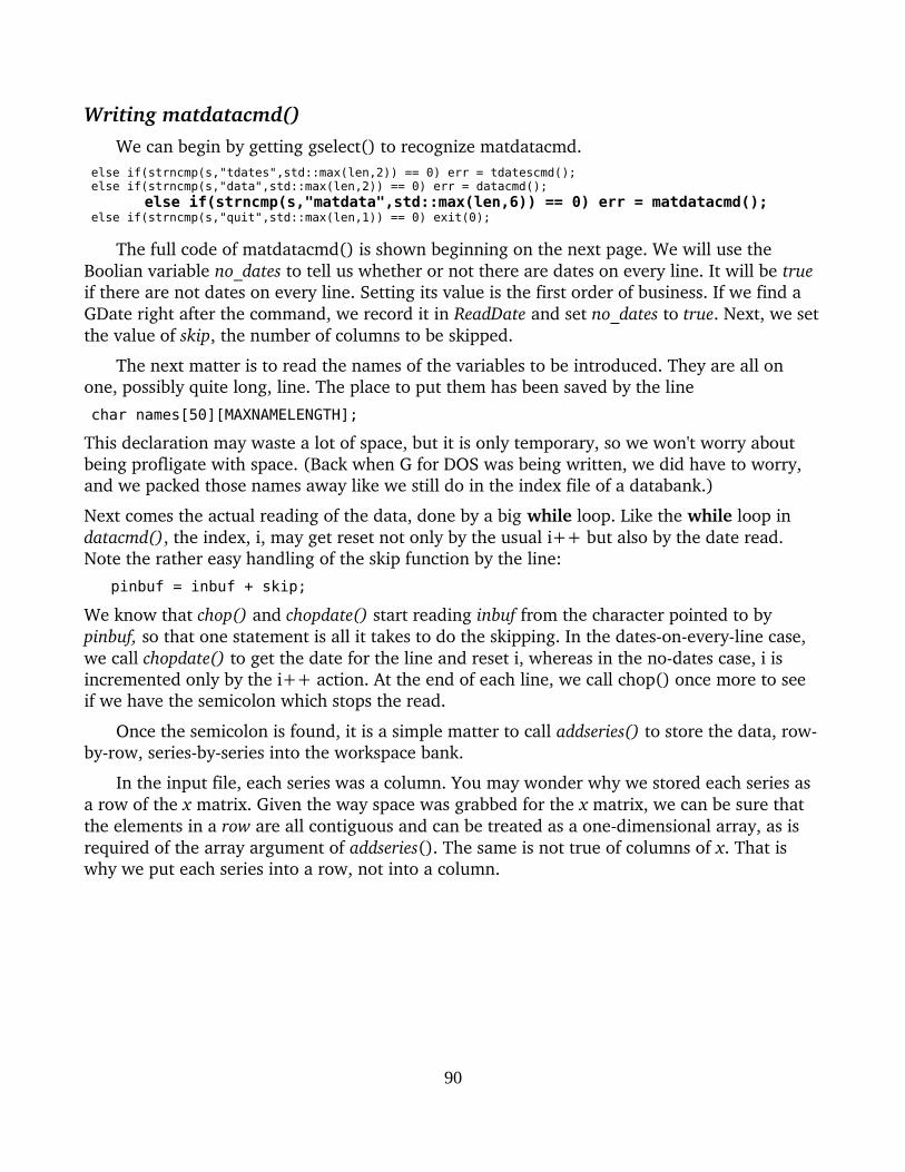
Writing matdatacmd()We can begin by getting gselect() to recognize matdatacmd.
else if(strncmp(s,"tdates",std::max(len,2)) == 0) err = tdatescmd(); else if(strncmp(s,"data",std::max(len,2)) == 0) err = datacmd();
else if(strncmp(s,"matdata",std::max(len,6)) == 0) err = matdatacmd(); else if(strncmp(s,"quit",std::max(len,1)) == 0) exit(0);
The full code of matdatacmd() is shown beginning on the next page. We will use the Boolian variable no_dates to tell us whether or not there are dates on every line. It will be true if there are not dates on every line. Setting its value is the first order of business. If we find a GDate right after the command, we record it in ReadDate and set no_dates to true. Next, we setthe value of skip, the number of columns to be skipped.
The next matter is to read the names of the variables to be introduced. They are all on one, possibly quite long, line. The place to put them has been saved by the line
char names[50][MAXNAMELENGTH];
This declaration may waste a lot of space, but it is only temporary, so we won't worry about being profligate with space. (Back when G for DOS was being written, we did have to worry, and we packed those names away like we still do in the index file of a databank.)
Next comes the actual reading of the data, done by a big while loop. Like the while loop in datacmd(), the index, i, may get reset not only by the usual i++ but also by the date read. Note the rather easy handling of the skip function by the line:
pinbuf = inbuf + skip;
We know that chop() and chopdate() start reading inbuf from the character pointed to by pinbuf, so that one statement is all it takes to do the skipping. In the datesoneveryline case, we call chopdate() to get the date for the line and reset i, whereas in the nodates case, i is incremented only by the i++ action. At the end of each line, we call chop() once more to see if we have the semicolon which stops the read.
Once the semicolon is found, it is a simple matter to call addseries() to store the data, rowbyrow, seriesbyseries into the workspace bank.
In the input file, each series was a column. You may wonder why we stored each series as a row of the x matrix. Given the way space was grabbed for the x matrix, we can be sure that the elements in a row are all contiguous and can be treated as a onedimensional array, as is required of the array argument of addseries(). The same is not true of columns of x. That is why we put each series into a row, not into a column.
90

short matdatacmd(){ char s[12]; // for reading dates char datum[MAXNAMELENGTH]; // for reading data points short ns;// number of series short skip; // number of places to be skipped at beginning of each line short choprtn,i,j,seriesnumber; short matdatartn; //Return value of this function float **x; // matrix of data GDate ReadDate; bool no_dates; // true if there are no dates on the data lines char names[50][MAXNAMELENGTH];
skip = 0; no_dates = false; // chop for a date choprtn = chopdate(s); if(choprtn == 'e') goto readnames; if (choprtn == 'a'){ if(s[0] == 'd'){ //Got the pseudo-date d no_dates = false; } //probably got a GDate else if (ReadDate.set(s) == OK){ // Got a starting date no_dates = true; } // Chop for skip count choprtn = chop(s); if(choprtn == 'n') skip = atoi(s); else { printg("Check that matdata command!\n"); return ERR; } }
readnames: nextline();
// ns becomes the Number of Series. Set it by counting the names. ns = 0; while ((chop(names[ns]) == 'a' && ns < 50)) ns++;
// Grab space for the data x = matrix(0,ns,0,nobs_ws);
// Read the data i = 0; if(no_dates){ i = ReadDate.ObNo(); } while(i < nobs_ws){ nextline(); pinbuf = inbuf + skip; // Deal with case of a date on every line if(!no_dates){ // Read the date for this line. choprtn = chopdate(s); if(ReadDate.set(s) != OK){ printg("Bad date: %s\n",s); matdatartn = ERR; goto closeup; } i = ReadDate.ObNo(); }
91

// Now read and store the row of data j = 0; while(j < ns){ choprtn = chopnumber(datum); if(choprtn == 'n'){ x[j][i] = atof(datum); j++; } else{ if(choprtn == 'e') printg("Unexpected end of line\n"); else printg("Bad datum %s\n",datum); matdatartn = ERR; goto closeup; } } // Increment i in case we are in the no-dates case. i++;
// Check for the ; that marks the end of the data. choprtn = chop(datum); if(choprtn == ';') break; }
// The data have been read. Now put them into the workspace bank. for(i = 0;i < ns; i++){ seriesnumber = addseries(names[i], x[i], ReadDate.freq,'y',nobs_ws); } matdatartn = OK;
closeup: free_matrix(x,0,ns,0); return matdatartn; }
To test this command, we augmented the matrix shown above to that shown below. It inputs the same data twice, once with dates on every line and once without. In the dates case, a D is appended to each variable name. After all the data has been read both ways, the two versions of each series are typed out. They should be the same. Just to test the reading of negative numbers, one of the entries has been made negative. The full test matrix is shown below.
This test is, of course, incomplete because all of the input is correct. One should test how the program behaves when the user makes various stupid mistakes. I have tried some, but I doubt that I have made all possible mistakes.
92

matdata 2009q1 21CoalElec CoalCoke CoalOthInd CoalTotal# U.S. Coal Consumption# (Thousand Short Tons)# Year and Electric Coke Other Total# Quarter Power Plants Industry###2009 January - March 236842 4398 12075 254383 April - June 216502 3402 10542 231110 July - September 244445 3450 11107 259621 October - December 235838 4076 11590 252363##2010 January - March 246445 4857 12600 264939 April - June 229469 5353 11914 247344 July - September 267943 5491 12284 286361 October - December 231195 5391 12490 249870##2011 January - March 234847 5188 12489 253541 April - June 223540 5392 11036 240611 July - September 261534 5407 11168 278638 October - December 208637 5447 -11543 226233 ;tdates 2009q1 2011q4type CoalElectype CoalCoketype CoalOthIndtype CoalTotal
matdata d 21CoalElecD CoalCokeD CoalOthIndD CoalTotalD# U.S. Coal Consumption# (Thousand Short Tons)# Year and Electric Coke Other Total# Quarter Power Plants Industry###2009 January - March 2009q1 236842 4398 12075 254383 April - June 2009q2 216502 3402 10542 231110 July - September 2009q3 244445 3450 11107 259621 October - December 2009q4 235838 4076 11590 252363##2010 January - March 2010q1 246445 4857 12600 264939 April - June 2010q2 229469 5353 11914 247344 July - September 2010q3 267943 5491 12284 286361 October - December 2010q4 231195 5391 12490 249870##2011 January - March 2011q1 234847 5188 12489 253541 April - June 2011q2 223540 5392 11036 240611 July - September 2011q3 261534 5407 11168 278638 October - December 2011q4 208637 5447 -11543 226233 ;type CoalElectype CoalElecDtype CoalCoketype CoalCokeDtype CoalOthIndtype CoalOthIndDtype CoalTotaltype CoalTotalD
93

Tutorial 10: The f CommandThe f command, as you will recall if you have ever used G for Windows, creates a new variableby arithmetic operations on existing variables. Some examples are:
f gdpd = gdp/gdp$f x = a*b*c + d*e/ff lgdp = @log(gdp)f x = (u*v + w*y)/z
All of the variables on the left are to be thought of as vectors. I had somewhat expected to be able to just throw the whole G7 code into Gwx, and that might have worked as far as the compiler is concerned. However, on reading the code, I found it tough going and much in needof explanation. So, as in previous tutorials, we will build it up stepbystep and hope to make the whole easily intelligible.
First Version – Arithmetic Only and No ParenthesesFor the first version, let's deal just with the four arithmetic operations – no logarithms,
exponentials or other functions – and righthand sides that do not involve parentheses, constants or lagw. In the above examples, only the first two would covered.
Clearly, most of the work is going to be in evaluating the expression on the righthand sideof the = sign. The ability to evaluate such expressions will prove useful in other contexts, so we will code it in a separate function, rhs() – standing for righthand side – and have the fcmd() function call rhs().
Let's think about what is involved in evaluating the function on the right of the second example. The pieces of the expression separated by + or – signs we will call terms. In the second example, the first term is a*b*c and the second term is d*e/f. We also need to remember the arithmetic operations which still need to be done. We will call the place for storing them the operator stack (or just the stack) and an integer indicating where the top of the stack is at any time the stack pointer (or just the pointer). The steps in evaluating the whole expression might then go something like this:
0. Put a + on the stack and set the pointer to point to it.1. Initialize a workspace vector, z, to zero.2. Read the first variable, here a, into a workspace vector called y.3. Check the top of the operator stack; since it is a + or , just copy y to a workspace vector
x.3. Read and record at the top of the stack the next operator (here a *) and increment the
stack pointer to point to it.4. Read the b variable into the workspace y.5. Check the top of the stack. Finding a *, multiply x by y elementbyelement and store the
results in x and decrement the stack pointer.
6. Read and record at the top of the stack the next operator (here a *) and increment the stack pointer to point to it
94

7. Read the c variable into the workspace y.8. Check the top of the stack. Finding a *, multiply x by y elementbyelement and store the
results in x and decrement the stack pointer.Note that steps 6 8 are exactly the same as steps 3 – 5. Repeat steps 6 8 until a + or – is encountered. The term is then finished. The pointer will then be pointing to the lowest element in the stack, which will be a + or .
9. The workspace x now contains a complete term. Add x to z or subtract x from z according to the operator pointed to by the pointer.
10. Put the + or – just found onto the stack at the position pointed to by the pointer. (It will always be the lowest position.)
11. Go back to step 2 to build up the next term. Continue this process until all terms have been added or subtracted.
9. Record the + or operator and add x into z.Repeat steps 18 to evaluate the d*e/f term in x.Recall the stored + operator and add x to z.
Note that no matter how many terms the expression may involve, we need only three workspace vectors. And we need to remember only two operators, namely whether the term we are working on will be added or subtracted from z and whether a series just read is to be multiplied by or divided into what is in workspace x.4
At the risk of repetition, let us be more explicit about remembering the operators. We will need a twoelement array of characters, which we will call op_stack (for operator stack) and a pointer to the element on top, which we will call osp. So that we can easily print out the op_stack as a string for debugging, we will give it three elements and initialize if like this:
char op_stack[3];op_stack[0] = '+';op_stack[1] = ' ';op_stack[2] = '\0';short osp = 0;
Note carefully that we start off with op_stack[0] = '+' and osp = 0.
Now we read a series into y. Forget for a moment that you know that this is the first series.Can we figure out what to do with it from just the operator on the top of the op_stack? Yes. If that operator is a * (or /), we multiply (or divide) elementbyelement what is already in x by the corresponding element of y and store the result in x. Otherwise, we simply copy y to x. So when we set out to evaluate the right side of f g = a*b*c + d*e/f, we first read the series a and, on not finding a * or / on top of the op_stack, we just copy a into a into x.
Then we look at the next element of the expression being evaluated and find a *. So we put the * into op_stack[1] and increment osp by 1 to be 1. Then we find that the next element
4 An expression like a*b/c*d is ambiguous; our procedure will give it the same value as a*b*d/c, which may not be what a user intended. We need not worry about this problem because, when we introduce parentheses, the user can say a*b/(c*d), if that is what is desired.
95
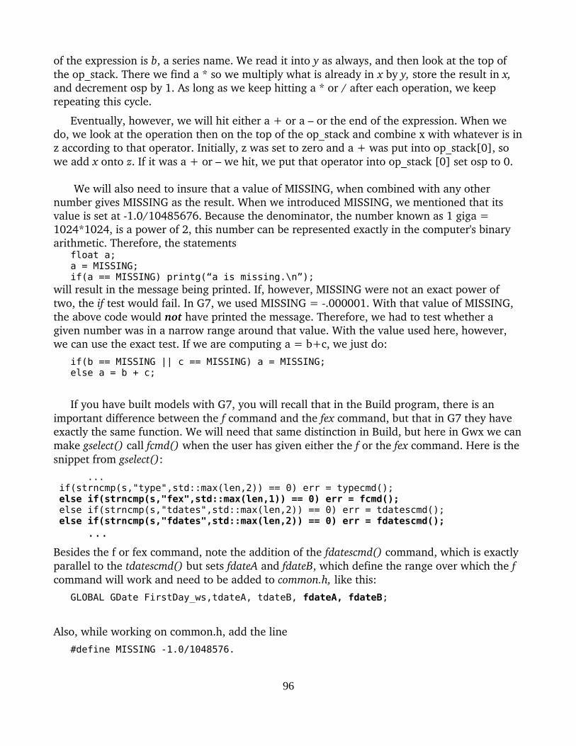
of the expression is b, a series name. We read it into y as always, and then look at the top of the op_stack. There we find a * so we multiply what is already in x by y, store the result in x, and decrement osp by 1. As long as we keep hitting a * or / after each operation, we keep repeating this cycle.
Eventually, however, we will hit either a + or a – or the end of the expression. When we do, we look at the operation then on the top of the op_stack and combine x with whatever is inz according to that operator. Initially, z was set to zero and a + was put into op_stack[0], so we add x onto z. If it was a + or – we hit, we put that operator into op_stack [0] set osp to 0.
We will also need to insure that a value of MISSING, when combined with any other
number gives MISSING as the result. When we introduced MISSING, we mentioned that its value is set at 1.0/10485676. Because the denominator, the number known as 1 giga = 1024*1024, is a power of 2, this number can be represented exactly in the computer's binary arithmetic. Therefore, the statements
float a;a = MISSING;if(a == MISSING) printg(“a is missing.\n”);
will result in the message being printed. If, however, MISSING were not an exact power of two, the if test would fail. In G7, we used MISSING = .000001. With that value of MISSING, the above code would not have printed the message. Therefore, we had to test whether a given number was in a narrow range around that value. With the value used here, however, we can use the exact test. If we are computing a = b+c, we just do:
if(b == MISSING || c == MISSING) a = MISSING;else a = b + c;
If you have built models with G7, you will recall that in the Build program, there is an important difference between the f command and the fex command, but that in G7 they have exactly the same function. We will need that same distinction in Build, but here in Gwx we canmake gselect() call fcmd() when the user has given either the f or the fex command. Here is the snippet from gselect():
... if(strncmp(s,"type",std::max(len,2)) == 0) err = typecmd(); else if(strncmp(s,"fex",std::max(len,1)) == 0) err = fcmd(); else if(strncmp(s,"tdates",std::max(len,2)) == 0) err = tdatescmd(); else if(strncmp(s,"fdates",std::max(len,2)) == 0) err = fdatescmd();
...
Besides the f or fex command, note the addition of the fdatescmd() command, which is exactly parallel to the tdatescmd() but sets fdateA and fdateB, which define the range over which the f command will work and need to be added to common.h, like this:
GLOBAL GDate FirstDay_ws,tdateA, tdateB, fdateA, fdateB;
Also, while working on common.h, add the line
#define MISSING -1.0/1048576.
96

I put it just below the #define SMALL, but the exact location is not important. Note that the numerator is 1.0, not just 1. The .0 causes the compiler to treat the numerator as a float or maybe a double. Without the .0, the division is done in integer arithmetic and the answer is a true zero, not at all what we want. The line
short fdatescmd();
needs to be added to common.h under in the GwxMain.cpp group.
The f command and funtions it calls will take up considerable space, so we'll put them in a new module we will call functions.cpp. (Remember, in Code::Blocks use File | New to put in a new module.) Also we add their prototypes to common.h, like this:
// in functions.cppshort fcmd();short rhs();
Here are fcmd() and our first version of rhs().#include "common.h"
short fcmd(){ char name[MAXNAMELENGTH]; char dump[MAXNAMELENGTH]; float *series; char choprtn; int rhsrtn; short obnoA, obnoB; int i,type,lasttype,go;
// Get the name of the variable being created choprtn = chop(name); if (choprtn != 'a'){
printg("I got a bad variable name in fcmd: %s\n",name); return ERR; }
series = vector(0,nobs_ws);
// Chop, really just to get past the = sign, but fuss if it is not there. choprtn = chop(dump); if (choprtn != '='){ printg("There was no = sign in the f or fex command.\n"); return ERR; } rhsrtn = rhs(series); if(rhsrtn == OK) short seriesnumber = addseries(name, series, fdateA.freq,'y',nobs_ws);
closeup: if(series) free_vector(series,0); geteol(); return rhsrtn; }
97
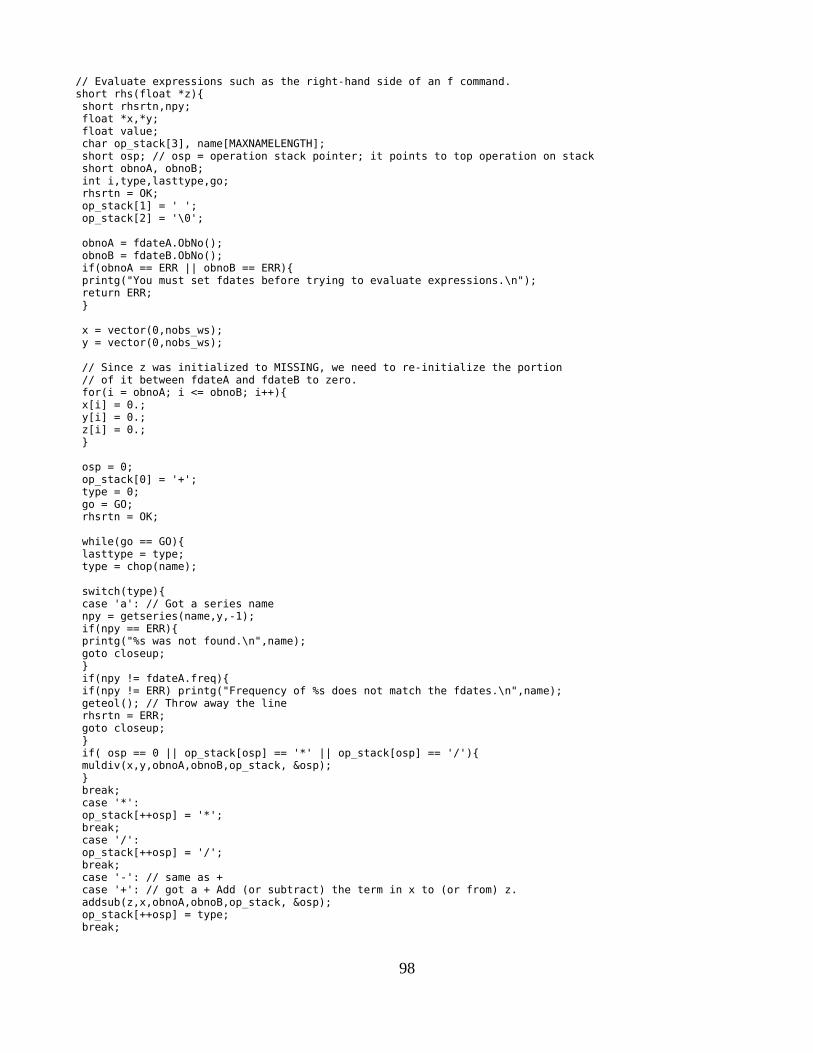
// Evaluate expressions such as the right-hand side of an f command.short rhs(float *z){ short rhsrtn,npy; float *x,*y; float value; char op_stack[3], name[MAXNAMELENGTH]; short osp; // osp = operation stack pointer; it points to top operation on stack short obnoA, obnoB; int i,type,lasttype,go; rhsrtn = OK; op_stack[1] = ' '; op_stack[2] = '\0';
obnoA = fdateA.ObNo(); obnoB = fdateB.ObNo(); if(obnoA == ERR || obnoB == ERR){ printg("You must set fdates before trying to evaluate expressions.\n"); return ERR; }
x = vector(0,nobs_ws); y = vector(0,nobs_ws);
// Since z was initialized to MISSING, we need to re-initialize the portion // of it between fdateA and fdateB to zero. for(i = obnoA; i <= obnoB; i++){ x[i] = 0.; y[i] = 0.; z[i] = 0.; }
osp = 0; op_stack[0] = '+'; type = 0; go = GO; rhsrtn = OK;
while(go == GO){ lasttype = type; type = chop(name);
switch(type){ case 'a': // Got a series name npy = getseries(name,y,-1); if(npy == ERR){ printg("%s was not found.\n",name); goto closeup; } if(npy != fdateA.freq){ if(npy != ERR) printg("Frequency of %s does not match the fdates.\n",name); geteol(); // Throw away the line rhsrtn = ERR; goto closeup; } if( osp == 0 || op_stack[osp] == '*' || op_stack[osp] == '/'){ muldiv(x,y,obnoA,obnoB,op_stack, &osp); } break; case '*': op_stack[++osp] = '*'; break; case '/': op_stack[++osp] = '/'; break; case '-': // same as + case '+': // got a + Add (or subtract) the term in x to (or from) z. addsub(z,x,obnoA,obnoB,op_stack, &osp); op_stack[++osp] = type; break;
98

case 'e': //end of line go = STOP; rhsrtn = OK; break; default: printg("Could not evaluate that expression.\n"); rhsrtn = ERR; goto closeup; } // end of big switch } // end of while // The call to addsub() after everything has been read addsub(z,x,obnoA,obnoB,op_stack,&osp); closeup: if(x) free_vector(x,0); if(y) free_vector(y,0);
return rhsrtn; }
short muldiv(float *x, float *y,short obnoA, short obnoB, char *op_stack, short *posp){ short i;
if(op_stack[*posp]== '*'){ // The previous operator was a * for(i = obnoA; i <= obnoB; i++){ if(x[i] == MISSING || y[i] == MISSING) x[i] = MISSING; else x[i] *= y[i]; } (*posp)--; } else if(op_stack[*posp]== '/'){ // The previous operator was a / for(i = obnoA; i <= obnoB; i++){ if(x[i] == MISSING || y[i] == MISSING) x[i] = MISSING; if(fabs(y[i]) < .0000001) x[i] = MISSING; else x[i] /= y[i]; } (*posp)--; } else{// We have the first component of a term. for(i = obnoA; i <= obnoB; i++) x[i] = y[i]; } return OK; }
short addsub(float *z, float *x,short obnoA, short obnoB, char *op_stack, short *posp){ short i;
if(op_stack[*posp] == '+'){ for(i = obnoA; i <= obnoB; i++){ if (z[i] == MISSING || x[i] == MISSING) z[i] = MISSING; else z[i] += x[i]; } (*posp)--; } else if(op_stack[*posp] == '-'){ for(i = obnoA; i <= obnoB; i++){ if (z[i] == MISSING || x[i] == MISSING) z[i] = MISSING; else z[i] -= x[i]; } (*posp)--; } return OK; }
99

That is a lot of somewhat complicated code all at once, but I believe that the preceding explanations make it all comprehensible. You should test it out. A number of tests can be built from the variable one which has been put in the workspace bank on startup, has a quarterly frequency, and the value 1.0 in all periods. You can do, for example:
fdates 1970.1 1970.3tdates 1970.1 1970.3f two = one + onetype twof five = two*two + 1type fivef x = five*five/two + onetype x
and so on. You can also use the real data in CoalUse.dat with, of course, different tdates and fdates. If you are curious to watch the sequence of calls, you can use the debugger. I spent a lot of time in it getting this to work correctly.
ConstantsIt is simple to provide for handling constants in the expression on the righthand side, as in
f x = 2.5*y – 3.0. We just add another case under the switch, like this:
case 'n': // got a number value = atof(name); for(i = obnoA; i <= obnoB; i++) y[i] = value; if( osp == 0 || op_stack[osp] == '*' || op_stack[osp] == '/') muldiv(x,y,obnoA,obnoB,op_stack, &osp); break;
ParenthesesAs was mentioned before, one of the beauties of C and C++ is that it is reentrant: a
function can all itself. That is NOT true in Fortran, where all arguments are passed by reference to where their values are stored. In my days as a Fortran programmer, it never occurred to me that it would be useful for a function to be able to call itself. But I was also never able write a program that would easily deal with parentheses. Indeed, a parenthesis just says to the computer, “You know how to evaluate expressions like this. Do so, and give me back a single number.” So to make rhs() handle parentheses, we just make it call itself, passingto the called version the y vector, which is the one we use for input of data. When control returns to the calling functions, the program treats the vector which has been calculated just asit would a vector that had been read. Here is the code:
100

case '(': // got an open parenthesis // Call rhs (recursively) to evaluate expression and put it in y // and treat as a series that has been read. rhsrtn = rhs(y); // The normal, healthy return is ')' if(rhsrtn != ')'){ printg("There was an error after that (\n"); geteol(); rhsrtn = ERR; go = STOP; goto closeup; } if(muldiv(x,y,obnoA,obnoB,op_stack, &osp) == ERR){ rhsrtn = ERR; goto closeup; } break;
Of course, when we enable the handling of an open parenthesis, we need also to handle the close parenthesis. That code is even easier. We want to stop the while loop that moves the computer through the expression. We do so by setting go equal to STOP, like this:
case ')': rhsrtn = ')'; go = STOP; break;
That's all there is to handling parentheses. Pretty simple.
The @log() and @exp functionsOne of the most useful transformations in economic statistics is taking the logarithm of all
values of a variable; the exponential, the inverse of the logarithm, is almost equally useful. We will now give Gwx the ability to use both to these functions. G7 currently has more than 60 such functions. Some change the frequency of a variable, one generates random normal deviates, another takes the sine of a variable, and so on with various functions which have been found useful at sometime. Here we will just do the natural logarithm, log(), and the exponential, exp(), to show such functions are done. When Gwx has become actually useful, we can come back and easily add more functions.
All of the functions are accessed by the user by putting an @ in front of a function name inan f command. For example, we could commands to Gwx like these;
f lgdp = @log(gdp)f xgdp = @exp(lgdp)
To deal with such command, we introduce the @ case in rhs() as shown in the bold type below: case ')': rhsrtn = ')'; go = STOP; break;
101
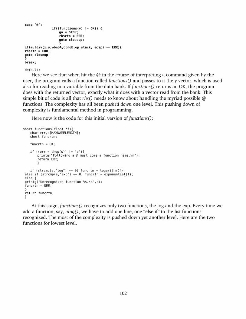
case '@':if((functions(y) != OK)) {
go = STOP;rhsrtn = ERR;goto closeup;}
if(muldiv(x,y,obnoA,obnoB,op_stack, &osp) == ERR){ rhsrtn = ERR; goto closeup; } break;
default:
Here we see that when hit the @ in the course of interpreting a command given by the user, the program calls a function called functions() and passes to it the y vector, which is usedalso for reading in a variable from the data bank. If functions() returns an OK, the program does with the returned vector, exactly what it does with a vector read from the bank. This simple bit of code is all that rhs() needs to know about handling the myriad possible @ functions. The complexity has all been pushed down one level. This pushing down of complexity is fundamental method in programming.
Here now is the code for this initial version of functions():
short functions(float *f){char err,s[MAXNAMELENGTH];short funcrtn;
funcrtn = OK;
if ((err = chop(s)) != 'a'){printg("Following a @ must come a function name.\n");return ERR;}
if (strcmp(s,"log") == 0) funcrtn = logarithm(f); else if (strcmp(s,"exp") == 0) funcrtn = exponential(f); else { printg("Unrecognized function %s.\n",s); funcrtn = ERR; } return funcrtn; }
At this stage, functions() recognizes only two functions, the log and the exp. Every time weadd a function, say, atoq(), we have to add one line, one “else if” to the list functions recognized. The most of the complexity is pushed down yet another level. Here are the two functions for lowest level.
102

short logarithm(float *f){ char s[MAXNAMELENGTH]; short obnoA,obnoB,i,err;
if ((err = chop(s)) != '(') goto error; // Get the argument for the logarithm by a call to rhs()
if ((err = rhs(f)) != ')') goto error;
obnoA = fdateA.ObNo(); obnoB = fdateB.ObNo(); for( i = obnoA; i <= obnoB; i++){ if(f[i] == MISSING) continue; else if (f[i] < 0) { printg("Cannot take the logarithm of %12.4f\n",f[i]); f[i] = MISSING; } else f[i] = log(f[i]); } return OK; error: return err; }
short exponential(float *f){ char s[MAXNAMELENGTH]; short obnoA,obnoB,i,err;
if ((err = chop(s)) != '(') goto error; // Get the argument for the exponential by a call to rhs()
if ((err = rhs(f)) != ')') goto error;
obnoA = fdateA.ObNo(); obnoB = fdateB.ObNo(); for( i = obnoA; i <= obnoB; i++){ if(f[i] == MISSING) continue; else f[i] = exp(f[i]); } return OK; error: return err; }
Note that in both cases, we (recursively) call rhs() to evaluate the expression whose logarithm or exponential is to be evaluate. Thus, the program can handle commands from the user like “f xxx = @log(aaa – bbb)”. Both functions look for MISSING and make the log and the exp of MISSING equal to MISSING, without any complaint. The logarithm function is also careful not to try to take the logarithm of negative numbers. If asked to do so, it complains andsets the value equal to MISSING.
With earlier C compilers, one had to be careful not to demand that the compiler's log or exp functions evaluate their functions for arguments outside the range of their capacities. Study of such documentation as I could find suggests that such care is no longer necessary. If the argument is outside the range in which the function gives valid answers, it does not crash the program but just returns some value called HUGE_VAL, which may be positive or negative.I suspect that outofrange calculations will usually show up as nonsense in the results. One can always check the validity of the logarithm of x by taking its exponential and checking that the value is x. Accordingly, I have not built in further safeguards on the values of the arguments to these functions.
With these functions working, you should be able to devise various programs to use and check the @log() and @exp() functions.
103
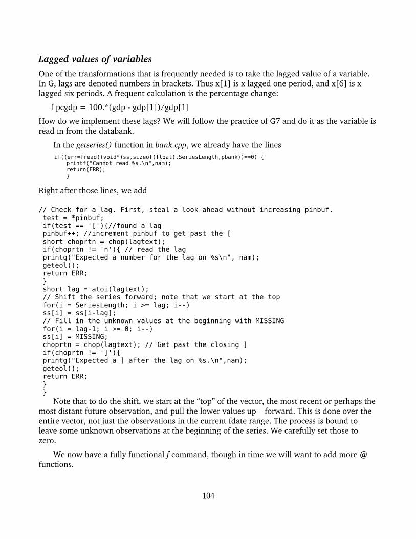
Lagged values of variablesOne of the transformations that is frequently needed is to take the lagged value of a variable. In G, lags are denoted numbers in brackets. Thus x[1] is x lagged one period, and x[6] is x lagged six periods. A frequent calculation is the percentage change:
f pcgdp = 100.*(gdp gdp[1])/gdp[1]
How do we implement these lags? We will follow the practice of G7 and do it as the variable isread in from the databank.
In the getseries() function in bank.cpp, we already have the lines if((err=fread((void*)ss,sizeof(float),SeriesLength,pbank))==0) {
printf("Cannot read %s.\n",nam); return(ERR); }
Right after those lines, we add
// Check for a lag. First, steal a look ahead without increasing pinbuf. test = *pinbuf; if(test == '['){//found a lag pinbuf++; //increment pinbuf to get past the [ short choprtn = chop(lagtext); if(choprtn != 'n'){ // read the lag printg("Expected a number for the lag on %s\n", nam); geteol(); return ERR; } short lag = atoi(lagtext); // Shift the series forward; note that we start at the top for(i = SeriesLength; i >= lag; i--) ss[i] = ss[i-lag]; // Fill in the unknown values at the beginning with MISSING for(i = lag-1; i >= 0; i--) ss[i] = MISSING; choprtn = chop(lagtext); // Get past the closing ] if(choprtn != ']'){ printg("Expected a ] after the lag on %s.\n",nam); geteol(); return ERR; } }
Note that to do the shift, we start at the “top” of the vector, the most recent or perhaps themost distant future observation, and pull the lower values up – forward. This is done over the entire vector, not just the observations in the current fdate range. The process is bound to leave some unknown observations at the beginning of the series. We carefully set those to zero.
We now have a fully functional f command, though in time we will want to add more @ functions.
104

Tutorial 11: Linear Regression: the r CommandGwx is, first and foremost, a program for doing linear regression. The first ten tutorials
were about infrastructure: setting up the windowing framework, making printg() work, writing chop() so that we can parse input to the program, providing for handling dates, gettingdata input into the program and displaying it in text form, and transforming the data via the f command. Finally, we are able to turn to basic linear regression by means of the r command.
The basic form of the command will be:
r y = x1, x2, …, xn
or
r y = ! x1, x2, …, xn
where y is a variable already in the data bank and x1, x2, …, xn are expressions involving variables in the data bank. In the first form, an intercept is automatically supplied. In the second form, with the !, no intercept is supplied. Thus, we could have:
r gdp = ex+im, @log(rtb)
but we cannot have
r ex+im = gdp, @log(rtb).
The reason for this limitation lies not in nature of regression itself but in the use to which the equation may be put when we come to model building. There, the left side must be a place into which the value calculated from the right side can be stored – an lvalue in C lingo. The name of a single variable is an lvalue. An expression involving, say a sum of two variables, is not an lvalue.
The rdates CommandThe range of dates over which a regression is to be calculated is specified by two Gdates:
rdateA and rdateB. If a third rdate, rdateC > rdateB, is given, then the predicted value is calculated over the entire range rdateA rdateC. This feature is quite important for examining the performance of the regression outside the period over which it was fit. If no rdateC is specified, it is set equat to rdateB. The rdates command therefore has the form:
rdates <rdateA> <rdateB> [rdateC]
where the < > indicate required arguments and [ ] indicate optional arguments. Here are some examples:
rdates 1980q1 2005q4 2012q3rdates 1980q1 2012q3rdates 2000.1 2011.1 2012.4
For coding the rdates command, we can begin in common.h and add among the prototypesthe lines shown here in bold:
105
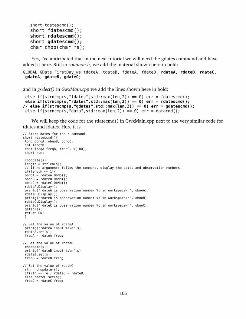
short tdatescmd();short fdatescmd();short rdatescmd();short gdatescmd();char chop(char *s);
Yes, I've anticipated that in the next tutorial we will need the gdates command and have added it here. Still in common.h, we add the material shown here in bold:
GLOBAL GDate FirstDay_ws,tdateA, tdateB, fdateA, fdateB, rdateA, rdateB, rdateC, gdateA, gdateB, gdateC;
and in gselect() in GwxMain.cpp we add the lines shown here in bold:
else if(strncmp(s,"fdates",std::max(len,2)) == 0) err = fdatescmd(); else if(strncmp(s,"rdates",std::max(len,2)) == 0) err = rdatescmd();// else if(strncmp(s,"gdates",std::max(len,2)) == 0) err = gdatescmd(); else if(strncmp(s,"data",std::max(len,2)) == 0) err = datacmd();
We will keep the code for the rdatecmd() in GwxMain.cpp next to the very similar code fortdates and fdates. Here it is.// Store dates for the r commandshort rdatescmd(){ long obnoA, obnoB, obnoC; int length; char freqA,freqB, freqC, s[100]; short rtn;
chopdate(s); length = strlen(s); // If no arguments follow the command, display the dates and observation numbers. if(length <= 1){ obnoA = rdateA.ObNo(); obnoB = rdateB.ObNo(); obnoC = rdateC.ObNo(); rdateA.Display(); printg("rdateA is observation number %d in workspace\n", obnoA); rdateB.Display(); printg("rdateB is observation number %d in workspace\n", obnoB); rdateC.Display(); printg("rdateC is observation number %d in workspace\n", obnoC); geteol(); return OK; }
// Set the value of rdateA printg("rdateA input %s\n",s); rdateA.set(s); freqA = rdateA.freq;
// Set the value of rdateB chopdate(s); printg("rdateB input %s\n",s); rdateB.set(s); freqB = rdateB.freq;
// Set the value of rdateC rtn = chopdate(s); if(rtn == 'e') rdateC = rdateB; else rdateC.set(s); freqC = rdateC.freq;
106
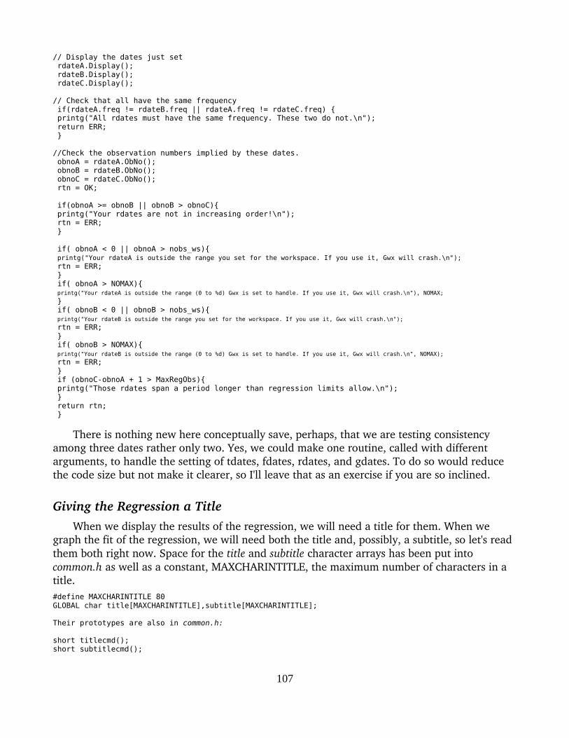
// Display the dates just set rdateA.Display(); rdateB.Display(); rdateC.Display();
// Check that all have the same frequency if(rdateA.freq != rdateB.freq || rdateA.freq != rdateC.freq) { printg("All rdates must have the same frequency. These two do not.\n"); return ERR; }
//Check the observation numbers implied by these dates. obnoA = rdateA.ObNo(); obnoB = rdateB.ObNo(); obnoC = rdateC.ObNo(); rtn = OK;
if(obnoA >= obnoB || obnoB > obnoC){ printg("Your rdates are not in increasing order!\n"); rtn = ERR; }
if( obnoA < 0 || obnoA > nobs_ws){ printg("Your rdateA is outside the range you set for the workspace. If you use it, Gwx will crash.\n"); rtn = ERR; } if( obnoA > NOMAX){ printg("Your rdateA is outside the range (0 to %d) Gwx is set to handle. If you use it, Gwx will crash.\n"), NOMAX; } if( obnoB < 0 || obnoB > nobs_ws){ printg("Your rdateB is outside the range you set for the workspace. If you use it, Gwx will crash.\n"); rtn = ERR; } if( obnoB > NOMAX){ printg("Your rdateB is outside the range (0 to %d) Gwx is set to handle. If you use it, Gwx will crash.\n", NOMAX); rtn = ERR; } if (obnoC-obnoA + 1 > MaxRegObs){ printg("Those rdates span a period longer than regression limits allow.\n"); } return rtn; }
There is nothing new here conceptually save, perhaps, that we are testing consistency among three dates rather only two. Yes, we could make one routine, called with different arguments, to handle the setting of tdates, fdates, rdates, and gdates. To do so would reduce the code size but not make it clearer, so I'll leave that as an exercise if you are so inclined.
Giving the Regression a TitleWhen we display the results of the regression, we will need a title for them. When we
graph the fit of the regression, we will need both the title and, possibly, a subtitle, so let's read them both right now. Space for the title and subtitle character arrays has been put into common.h as well as a constant, MAXCHARINTITLE, the maximum number of characters in a title.#define MAXCHARINTITLE 80GLOBAL char title[MAXCHARINTITLE],subtitle[MAXCHARINTITLE];
Their prototypes are also in common.h:
short titlecmd();short subtitlecmd();
107
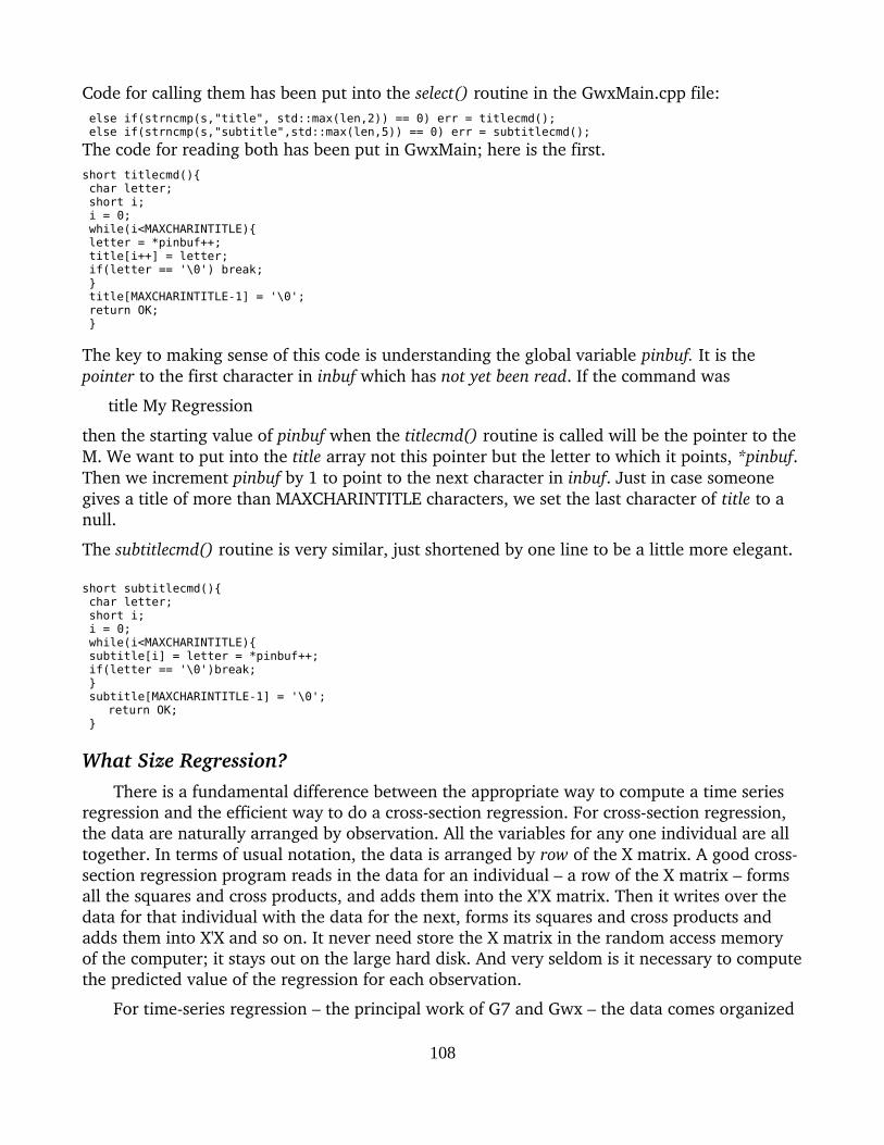
Code for calling them has been put into the select() routine in the GwxMain.cpp file: else if(strncmp(s,"title", std::max(len,2)) == 0) err = titlecmd(); else if(strncmp(s,"subtitle",std::max(len,5)) == 0) err = subtitlecmd();
The code for reading both has been put in GwxMain; here is the first.short titlecmd(){ char letter; short i; i = 0; while(i<MAXCHARINTITLE){ letter = *pinbuf++; title[i++] = letter; if(letter == '\0') break; } title[MAXCHARINTITLE-1] = '\0'; return OK; }
The key to making sense of this code is understanding the global variable pinbuf. It is the pointer to the first character in inbuf which has not yet been read. If the command was
title My Regression
then the starting value of pinbuf when the titlecmd() routine is called will be the pointer to the M. We want to put into the title array not this pointer but the letter to which it points, *pinbuf. Then we increment pinbuf by 1 to point to the next character in inbuf. Just in case someone gives a title of more than MAXCHARINTITLE characters, we set the last character of title to a null.
The subtitlecmd() routine is very similar, just shortened by one line to be a little more elegant.
short subtitlecmd(){ char letter; short i; i = 0; while(i<MAXCHARINTITLE){ subtitle[i] = letter = *pinbuf++; if(letter == '\0')break; } subtitle[MAXCHARINTITLE-1] = '\0';
return OK; }
What Size Regression?There is a fundamental difference between the appropriate way to compute a time series
regression and the efficient way to do a crosssection regression. For crosssection regression, the data are naturally arranged by observation. All the variables for any one individual are all together. In terms of usual notation, the data is arranged by row of the X matrix. A good crosssection regression program reads in the data for an individual – a row of the X matrix – forms all the squares and cross products, and adds them into the X'X matrix. Then it writes over the data for that individual with the data for the next, forms its squares and cross products and adds them into X'X and so on. It never need store the X matrix in the random access memory of the computer; it stays out on the large hard disk. And very seldom is it necessary to computethe predicted value of the regression for each observation.
For timeseries regression – the principal work of G7 and Gwx – the data comes organized
108
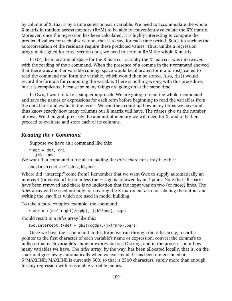
by column of X, that is by a time series on each variable. We need to accommodate the whole X matrix in random access memory (RAM) to be able to conveniently calculate the X'X matrix. Moreover, once the regression has been calculated, it is highly interesting to compute the predicted values for each observation, that is to say, for each time period. Statistics such as theautocorrelation of the residuals require these predicted values. Thus, unlike a regression program designed for crosssection data, we need to store in RAM the whole X matrix.
In G7, the allocation of space for the X matrix – actually the X' matrix – was interwoven with the reading of the r command. When the presence of a comma in the r command showed that there was another variable coming, space would be allocated for it and rhs() called to read the command and form the variable, which would then be stored. Also, rhs() would record the formula for computing the variable. There is nothing wrong with this procedure, but it is complicated because so many things are going on at the same time.
In Gwx, I want to take a simpler approach. We are going to read the whole r command and save the names or expressions for each term before beginning to read the variables from the data bank and evaluate the terms. We can then count up how many terms we have and thus know exactly how many columns our X matrix will have. The rdates give us the number of rows. We then grab precisely the amount of memory we will need for X, and only then proceed to evaluate and store each of its columns.
Reading the r CommandSuppose we have an r command like this:
r abc = def, ghi, jkl, mnoWe want that command to result in loading the titles character array like this:
abc,intercept,def,ghi,jkl,mno
Where did “intercept” come from? Remember that we want Gwx to supply automatically an intercept (or constant) term unless the = sign is followed by an ! point. Note that all spaces have been removed and there is no indication that the input was on two (or more) lines. The titles array will be used not only for creating the X matrix but also for labeling the output and writing the .sav files which are used in model building.
To take a more complex example, the command
r abc = ((def + ghi)/dgdp), (jkl*mno), pqrs
should result in a titles array like this:
abc,intercept,((def + ghi)/dgdp),(jkl*mno),pqrs
Once we have the r command in this form, we run through the titles array, record a pointer to the first character of each variable's name or expression, convert the comma's to nulls so that each variable's name or expression is a Cstring, and in the process count how many variables we have. The titles array, by the way, has been allocated locally, that is, on the stack and goes away automatically when we exit rcmd. It has been dimensioned at 5*MAXLINE; MAXLINE is currently 500, so that is 2500 characters, surely more than enough for any regression with reasonable variable names.
109
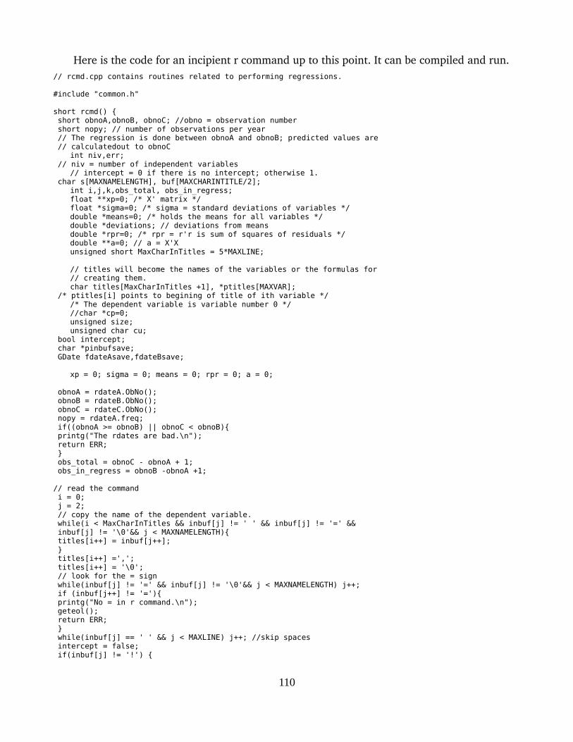
Here is the code for an incipient r command up to this point. It can be compiled and run.// rcmd.cpp contains routines related to performing regressions.
#include "common.h"
short rcmd() { short obnoA,obnoB, obnoC; //obno = observation number short nopy; // number of observations per year // The regression is done between obnoA and obnoB; predicted values are // calculatedout to obnoC
int niv,err; // niv = number of independent variables
// intercept = 0 if there is no intercept; otherwise 1. char s[MAXNAMELENGTH], buf[MAXCHARINTITLE/2];
int i,j,k,obs_total, obs_in_regress;float **xp=0; /* X' matrix */float *sigma=0; /* sigma = standard deviations of variables */double *means=0; /* holds the means for all variables */double *deviations; // deviations from meansdouble *rpr=0; /* rpr = r'r is sum of squares of residuals */double **a=0; // a = X'Xunsigned short MaxCharInTitles = 5*MAXLINE;
// titles will become the names of the variables or the formulas for// creating them.char titles[MaxCharInTitles +1], *ptitles[MAXVAR];
/* ptitles[i] points to begining of title of ith variable *//* The dependent variable is variable number 0 *///char *cp=0;unsigned size;unsigned char cu;
bool intercept; char *pinbufsave; GDate fdateAsave,fdateBsave;
xp = 0; sigma = 0; means = 0; rpr = 0; a = 0;
obnoA = rdateA.ObNo(); obnoB = rdateB.ObNo(); obnoC = rdateC.ObNo(); nopy = rdateA.freq; if((obnoA >= obnoB) || obnoC < obnoB){ printg("The rdates are bad.\n"); return ERR; } obs_total = obnoC - obnoA + 1; obs_in_regress = obnoB -obnoA +1;
// read the command i = 0; j = 2; // copy the name of the dependent variable. while(i < MaxCharInTitles && inbuf[j] != ' ' && inbuf[j] != '=' && inbuf[j] != '\0'&& j < MAXNAMELENGTH){ titles[i++] = inbuf[j++]; } titles[i++] =','; titles[i++] = '\0'; // look for the = sign while(inbuf[j] != '=' && inbuf[j] != '\0'&& j < MAXNAMELENGTH) j++; if (inbuf[j++] != '='){ printg("No = in r command.\n"); geteol(); return ERR; } while(inbuf[j] == ' ' && j < MAXLINE) j++; //skip spaces intercept = false; if(inbuf[j] != '!') {
110
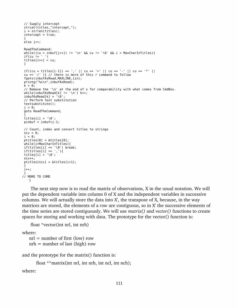
// Supply intercept strcat(titles,"intercept,"); i = strlen(titles); intercept = true; } else j++;
ReadTheCommand: while((cu = inbuf[j++]) != '\n' && cu != '\0' && i < MaxCharInTitles){ if(cu != ' ') titles[i++] = cu; }
if((cu = titles[i-1]) == ',' || cu == '+' || cu == '-' || cu == '*' || cu == '/' ){ // there is more of this r command to follow fgets(inbufAsRead,MAXLINE,iin); printg("%s\n",inbufAsRead); k = 0; // Remove the '\n' at the end of s for comparability with what comes from CmdBox. while(inbufAsRead[k] != '\n') k++; inbufAsRead[k] = '\0'; // Perform text substitution textsubstitute(); j = 0; goto ReadTheCommand; } titles[i] = '\0'; pinbuf = inbuf+j-1;
// Count, index and convert titles to strings niv = 0; i = 0; ptitles[0] = &titles[0]; while(i<MaxCharInTitles){ if(titles[i] == '\0') break; if(titles[i] == ','){ titles[i] = '\0'; niv++; ptitles[niv] = &titles[i+1]; } i++; }// MORE TO COME
}
The next step now is to read the matrix of observations, X in the usual notation. We will put the dependent variable into column 0 of X and the independent variables in successive columns. We will actually store the data into X', the transpose of X, because, in the way matrices are stored, the elements of a row are contiguous, so in X' the successive elements of the time series are stored contiguously. We will use matrix() and vector() functions to create spaces for storing and working with data. The prototype for the vector() function is:
float *vector(int nrl, int nrh)
where: nrl = number of first (low) row
nrh = number of last (high) row
and the prototype for the matrix() function is:
float **matrix(int nrl, int nrh, int ncl, int nch);
where:
111
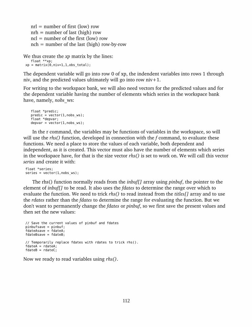
nrl = number of first (low) rownrh = number of last (high) rowncl = number of the first (low) rownch = number of the last (high) rowbyrow
We thus create the xp matrix by the lines:float **xp;
xp = matrix(0,niv+1,1,obs_total);
The dependent variable will go into row 0 of xp, the indendent variables into rows 1 through niv, and the predicted values ultimately will go into row niv+1.
For writing to the workspace bank, we will also need vectors for the predicted values and for the dependent variable having the number of elements which series in the workspace bank have, namely, nobs_ws:
float *predic;predic = vector(1,nobs_ws);float *depvar;depvar = vector(1,nobs_ws);
In the r command, the variables may be functions of variables in the workspace, so will will use the rhs() function, developed in connection with the f command, to evaluate these functions. We need a place to store the values of each variable, both dependent and independent, as it is created. This vector must also have the number of elements which series in the workspace have, for that is the size vector rhs() is set to work on. We will call this vectorseries and create it with: float *series; series = vector(1,nobs_ws);
The rhs() function normally reads from the inbuf[] array using pinbuf, the pointer to the element of inbuf[] to be read. It also uses the fdates to determine the range over which to evaluate the function. We need to trick rhs() to read instead from the titles[] array and to use the rdates rather than the fdates to determine the range for evaluating the function. But we don't want to permanently change the fdates or pinbuf, so we first save the present values and then set the new values:
// Save the current values of pinbuf and fdates pinbufsave = pinbuf; fdateAsave = fdateA; fdateBsave = fdateB;
// Temporarily replace fdates with rdates to trick rhs(). fdateA = rdateA; fdateB = rdateC;
Now we ready to read variables using rhs().
112

// Read in the variables for(i = 0; i <= niv; i++){ if(i == 1 && intercept) { for(j = 1;j <= obs_total;j++) xp[1][j] = 1.0; } else { pinbuf = ptitles[i]; rhs(series); for(j = 1;j <= obs_total;j++) xp[i][j] = series[obnoA+j-1]; } if(i == 0){ // Store the dependent variable in depvar for(j=1; j<= nobs_ws; j++) depvar[j] = series[j]; } }
pinbuf = pinbufsave; fdateA = fdateAsave; fdateB = fdateBsave;
We have now read the X matrix. To check our coding, it is a good idea to display it with code we will later want to eliminate.
// Debug printg("The X matrix:\n");
for(j = 1;j <= obs_total;j++){ for(i = 0; i <= niv; i++) printg(" %12.4f",xp[i][j]); printg("\n"); } //End Debug
It may be useful to review for a moment the process of solving the normal equations, (X'X)b = X'y. It will simplify the programming a bit to put the dependent variable, y, into the 0th column of the X matrix. We can illustrate the method by using the numerical example of Chapter 1 of The Craft of Economic Modeling. In that example, the matrix of observations, (y,X), is
17 1 10 510 1 5 1 12 1 0 616 1 10 3 20 1 0 10
The (y X)'(y X) matrix is then
1189.00 75 380 41575.00 5 25 25
380.00 25 225 85415.00 25 85 171
The process of solving the normal equations (X'X)b = X'y is illustrated in the following table. In each panel, the pivot element for moving to the next panel is marked by heavy
113
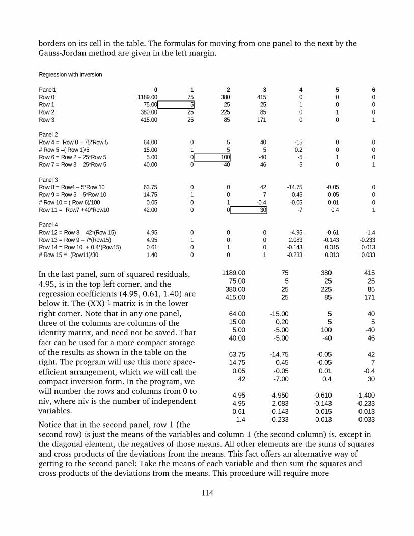
borders on its cell in the table. The formulas for moving from one panel to the next by the GaussJordan method are given in the left margin.
In the last panel, sum of squared residuals,4.95, is in the top left corner, and theregression coefficients (4.95, 0.61, 1.40) arebelow it. The (X'X)1 matrix is in the lowerright corner. Note that in any one panel,three of the columns are columns of theidentity matrix, and need not be saved. Thatfact can be used for a more compact storageof the results as shown in the table on theright. The program will use this more spaceefficient arrangement, which we will call thecompact inversion form. In the program, wewill number the rows and columns from 0 toniv, where niv is the number of independentvariables.
Notice that in the second panel, row 1 (thesecond row) is just the means of the variables and column 1 (the second column) is, except in the diagonal element, the negatives of those means. All other elements are the sums of squaresand cross products of the deviations from the means. This fact offers an alternative way of getting to the second panel: Take the means of each variable and then sum the squares and cross products of the deviations from the means. This procedure will require more
114
Regression with inversion
Panel1 0 1 2 3 4 5 6Row 0 1189.00 75 380 415 0 0 0Row 1 75.00 5 25 25 1 0 0Row 2 380.00 25 225 85 0 1 0Row 3 415.00 25 85 171 0 0 1
Panel 2Row 4 = Row 0 – 75*Row 5 64.00 0 5 40 -15 0 0# Row 5 =( Row 1)/5 15.00 1 5 5 0.2 0 0Row 6 = Row 2 – 25*Row 5 5.00 0 100 -40 -5 1 0Row 7 = Row 3 – 25*Row 5 40.00 0 -40 46 -5 0 1
Panel 3Row 8 = Row4 – 5*Row 10 63.75 0 0 42 -14.75 -0.05 0Row 9 = Row 5 – 5*Row 10 14.75 1 0 7 0.45 -0.05 0# Row 10 = ( Row 6)/100 0.05 0 1 -0.4 -0.05 0.01 0Row 11 = Row7 +40*Row10 42.00 0 0 30 -7 0.4 1
Panel 4Row 12 = Row 8 – 42*(Row 15) 4.95 0 0 0 -4.95 -0.61 -1.4Row 13 = Row 9 – 7*(Row15) 4.95 1 0 0 2.083 -0.143 -0.233Row 14 = Row 10 + 0.4*(Row15) 0.61 0 1 0 -0.143 0.015 0.013# Row 15 = (Row11)/30 1.40 0 0 1 -0.233 0.013 0.033
1189.00 75 380 41575.00 5 25 25
380.00 25 225 85415.00 25 85 171
64.00 -15.00 5 4015.00 0.20 5 55.00 -5.00 100 -40
40.00 -5.00 -40 46
63.75 -14.75 -0.05 4214.75 0.45 -0.05 70.05 -0.05 0.01 -0.4
42 -7.00 0.4 30
4.95 -4.950 -0.610 -1.4004.95 2.083 -0.143 -0.2330.61 -0.143 0.015 0.0131.4 -0.233 0.013 0.033

computation but will generally give better control of rounding error. The reason is that when numbers of similar size are subtracted, the can be a striking loss of accuracy. For example, suppose that we know two numbers accurate to eight significant figures: 1723549.9 and 1723549.2. If we take their difference, we get 0.7, but we know it accurate to only one significant figure! This subtraction of numbers very close together is exactly what often happens in the first pivot operation of inverting X'X. In those cases, that second step of the inversion is much more accurately reached by first taking the means of the variables and then the deviations from means, and the sums of squares and cross products of the deviations. That is what we will do if the regression has an intercept – as it usually does.
We will in any case need the means, so we begin by computing them. This is also a good time to check for missing observations. // Find the means and check for missing observations means = dvector(0,niv); deviations = dvector(0,niv); for (i = 0;i <= niv; i++){ means[i] = 0; for(j = 1; j <= obs_in_regress;j++){ if(xp[i][j] == MISSING) printg("Missing value in variable %d, observation %d",i,j); means[i] += xp[i][j]; } means[i] = means[i]/obs_in_regress; }
// Debug for (i = 0; i <= niv; i++) printg(" %2d %-20s %10.1f\n",i, ptitles[i],means[i]);
Now we form the X'X matrix, using the deviations from means if there is an intercept. Because X'X is symmetric, we will first compute only the elements on and above the diagonal. Then we will come back and copy each abovediagonal element to the symmetrically placed belowdiagonal element. // Form the X'X matrix, calling it a. a = dmatrix(0,niv,0,niv); sigma = vector(0,niv);
rpr = dvector(0,niv);
for (i = 0; i <= niv; i++) {for (j = i; j <= niv; j++)
a[i][j] = 0.0;}
if(intercept){for(k=0;k<obs_in_regress;k++){
for (j = 0;j <= niv; j++)deviations[j] = xp[j][k] - means[j];
for(i = 0;i <=niv; i++){if(i==1) continue;for(j = i; j <= niv; j++)
a[i][j] += deviations[i]*deviations[j];}
}for (i = 0; i <= niv; i++) {
for (j = i; j <= niv; j++)a[j][i] = a[i][j];
}
for (i = 0; i <= niv; i++)
115

sigma[i] = safesqrt(a[i][i]/obs_in_regress);
/* fix the 1'th row and column of 'a' as they would be afterthe pivot on the intercept. */
for (i = 0;i<=niv;i++){a[1][i] = means[i];a[i][1] = -means[i];}
a[1][1] = 1./obs_in_regress;}
else{ /* no intercept */for(i = 0;i <=niv; i++) {
for(j = i; j <= niv; j++) {for(k=0;k<obs_in_regress;k++)
a[i][j] += xp[i][k]*xp[j][k];a[j][i] = a[i][j];}
sigma[i] = safesqrt((a[i][i]-obs_in_regress*means[i]*means[i])/obs_in_regress);
}}
We have several times used safesqrt(). It has been written as an inline function in common.h:inline double safesqrt(const double f){
if(f < 0) return MISSING;return sqrt( f );}
Now we call the inversion() routine to get the regression coefficients. We will come back tohave a look at the details of inversion.
err = inversion(xp,a,means,niv,ptitles,obs_in_regress,obs_total,intercept,sigma,xp[niv+1],1,rpr);
We can now compute some of supplementary statistics describing the regression such as the predicted values, the R2, the Mean Absolute Percentage Error (MAPE), the autocorrelation coefficient of the residuals (rho), the Marginal Explanatory Value (mexval) of each variable, the elasticity of the dependent variable with respect to each independent variable (evaluated at the means of the variables) and the Normalized Residuals (NorRes) – which is the sum of squared residuals after the introduction of each variable divided by the sum of squared residuals after the introduction of all variables. G7 computes a number of other results, such asRbarSq, the muchabused and generally invalid tstatistics, F statistics after the introduction of each variable, the JarqueBera statistic and the leverage variable. It will be easy enough to come back and add these calculations, but we have the basics of what we need for practical model building. The coding is straightforward and requires no more explanation than is provided by the comments in the code.
// Compute predicted values, residuals, Durbin-Watson, rho for(i=1; i<=nobs_ws; i++){ predic[i] = MISSING; }
// Calculate predicted values, Mean Absolute Percentage Error (mape),// Autocorrelation of errors (rho), and Durbin-Watson statistic (dw) float dw,resid,lresid,pred,ssr,rho,mape,rsq,rbarsq;
116

mape = 0.; ssr = 0; dw = 0;
for (i = 1;i <= obs_in_regress; i++){pred = 0;for (j = 1; j <= niv; j++)
pred += a[j][0]*xp[j][i];// Align with workspace bankpredic[i+obnoA-1] = pred;resid = pred - xp[0][i];ssr += resid*resid;if(fabs(xp[0][i]) > 0)
mape += fabs(resid/xp[0][i]);if(i > 1){
lresid = resid - lresid;dw += lresid*lresid;}
lresid = resid;}
// Durbin-Watson statistic if(ssr > 0.) dw /= ssr;
else dw = 2;rho = 1.- 0.5*dw;// Mean absolute percentage errormape /= obs_in_regress;
// Print regression results float mexval,student, norresid, sigma_sq, see, elas; // ssr = Sum of Squared Residuals sigma_sq = ssr/(obs_in_regress - niv); see = safesqrt(ssr/obs_in_regress); rsq = 1. - ssr/rpr[1];
// Print the results. // Center the title j = (MAXCHARINTITLE - strlen(title))/2;
for(i=1;i<j;i++) buf[i] = ' '; buf[0] =':'; buf[j] = '\0'; printg("%s",buf); printg(" %s \n",title);
printg("SEE = %10.1f RSQ = %8.3f RHO = %8.3f DW = %8.3f\n",see,rsq,rho,dw);
printg(" Variable name RegCoef Mexval Elas NorRes Means\n");
for (i = 1;i <= niv;i++){ mexval =100.*(safesqrt(1.+ (a[i][0]*a[i][0]/
(a[i][i]*a[0][0])))-1.);
student = a[i][0]/safesqrt(a[i][i]*sigma_sq);elas = norresid = 0;if(means[0]!=0) elas = a[i][0]*means[i]/means[0];if(rpr[niv] > 0) norresid = rpr[i]/rpr[niv];if(norresid > 9999.99) norresid = 9999.99;printg(" %2d %-20s ",i,ptitles[i]);printg(" %10.5f %7.1f",a[i][0],mexval);printg(" %6.2f %7.2f %9.2f\n",elas,norresid,means[i]);
//if(i == 0 && showt) printg(" %7.3f",student);}
// Put the predicted values, residuals, and dependent variable into the workspace. // Prototype:
// short addseries(char *nam, float *series, short nopy, char wrindex_flag, short SeriesLength); err = addseries("depvar",depvar,nopy,'y' ,nobs_ws); err = addseries("predic",predic,nopy,'y',nobs_ws);
// Release the memory we grabbed for matrices and vectors.
117

// prototype:void free_matrix(float **m, int nrl, int nrh, int ncl) free_matrix(xp,0,niv,1); free_dmatrix(a,0,niv,0); free_vector(series,1); free_vector(depvar,1); free_vector(predic,1);
free_dvector(means,0); free_vector(sigma,0);
free_dvector(rpr,0,);
return OK; }
Now let's have a look at the inversion() routine. It is taken with almost no change from G7,int inversion(float **xp,double **a,double *means,int niv,
char *ptitles[],int obs_in_regress, int obs_total,int intercept,float *sigma, float *vresid,int nStackedReg, double *rpr){int i,j,k,err;double pivot;if(intercept >= 0) rpr[intercept] = a[0][0]; /* rpr = r'r is sum of squared resids */for (i = intercept+1;i<=niv;i++){
/* divide pivot row by pivot element */if(a[i][i] <= 0){
printg("Variable %d is a linear combination of preceeding variables.\n",i);return(ERR);}
pivot = 1.;pivot = pivot/a[i][i];a[i][i] = 1.;for (j = 0;j<=niv;j++)
a[i][j] = a[i][j]*pivot;/* row reduce non-pivot rows */for (j = 0; j <= niv; j++){
if(j==i)continue;pivot = a[j][i];a[j][i] = 0.;for (k = 0; k <= niv; k++)
a[j][k] -= a[i][k]*pivot;}
rpr[i] = a[0][0];}
err = OK;
return(err); }
We need to add a few lines to common.h:
short titlecmd();short subtitlecmd();
. . . .
// in rcmd.cppshort rcmd();int inversion(float **xp,double **a,double *means,int niv,
char *ptitles[],int obs_in_regress, int obs_total,bool intercept,float *sigma, float *vresid,int nStackedReg, double *rpr);
In the select() routine in the GwxMain.cpp file, we need to insert
else if(strncmp(s,"title", std::max(len,2)) == 0) err = titlecmd(); else if(strncmp(s,"subtitle",std::max(len,5)) == 0) err = subtitlecmd(); else if(strcmp(s,"r") == 0) err = rcmd();
118
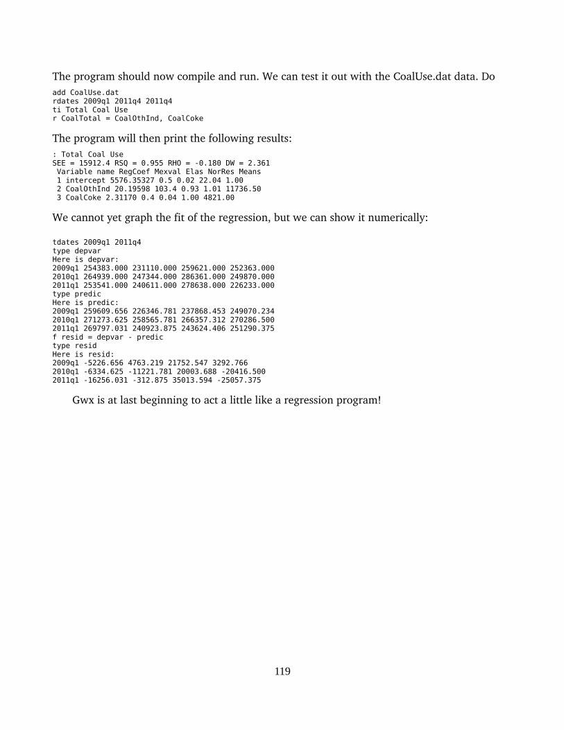
The program should now compile and run. We can test it out with the CoalUse.dat data. Doadd CoalUse.datrdates 2009q1 2011q4 2011q4ti Total Coal User CoalTotal = CoalOthInd, CoalCoke
The program will then print the following results:: Total Coal Use SEE = 15912.4 RSQ = 0.955 RHO = -0.180 DW = 2.361 Variable name RegCoef Mexval Elas NorRes Means 1 intercept 5576.35327 0.5 0.02 22.04 1.00 2 CoalOthInd 20.19598 103.4 0.93 1.01 11736.50 3 CoalCoke 2.31170 0.4 0.04 1.00 4821.00
We cannot yet graph the fit of the regression, but we can show it numerically:
tdates 2009q1 2011q4 type depvar Here is depvar: 2009q1 254383.000 231110.000 259621.000 252363.000 2010q1 264939.000 247344.000 286361.000 249870.000 2011q1 253541.000 240611.000 278638.000 226233.000 type predic Here is predic: 2009q1 259609.656 226346.781 237868.453 249070.234 2010q1 271273.625 258565.781 266357.312 270286.500 2011q1 269797.031 240923.875 243624.406 251290.375 f resid = depvar - predic type resid Here is resid: 2009q1 -5226.656 4763.219 21752.547 3292.766 2010q1 -6334.625 -11221.781 20003.688 -20416.500 2011q1 -16256.031 -312.875 35013.594 -25057.375
Gwx is at last beginning to act a little like a regression program!
119
Tutorial 12. GraphsThe origins of G's graphics go back long before the availability of computer screens and
laser printers for their display. Around 1962, I saw a line printer that could print only capital letters and numerals drawing helpful graphs by plunking down an X in the appropriate columnof the sprocketfed paper. The program had been written by a Harvard physics professor, and Iquickly wrote a program using the same idea for use with economic data. I spent many an hour connecting the dots. It was not until the PC revolution twenty years later that we were able to draw continuous lines on the screen and on paper. The DeSmet C compiler first made this step possible, and then the Borland C compiler 1.5 gave us for the first time the possibility of beautiful, multicolored graphs drawn on a beautiful deepblue background. These graphs were drawn, I should emphasize, under the DOS operating system, not under Windows. Drawing them with Borland Builder under Windows was yet another step. These graphs were perhaps more versatile than the DOS graphs, but not more beautiful.
Possibly we should use some opensource C++ graphics package, such as PLplot. But our graphs are basically simple, just sequences of straight lines. Most of the programming goes intoproviding the interface between the user and the the graphicdrawing functions and between the rest of the program and those functions. Thus, little would be gained by more evolved graphics routines than offered by wxWidgets. Indeed, we use only a small fraction of what wxWidgets provides. Moreover, we keep the greatest flexibility for future development by building from the basics, as we shall do.
Our first objective in this tutorial is simply to put a title on the screen and, below it, a graph of several series. We will not at first worry about controlling or marking the vertical scale, nor about providing a legend for the graph, nor about saving the graph. All that will come later.
Auxiliary Graphing Commands I: gdates Before we can draw graphs, we need to introduce the gdates. As with rdates, there are
three gdates: gdateA where the graph begins, gdateB where a vertical line is drawn, and gdateC, where the graph ends. In graphing regression results, the vertical line divides the period of the fit from the test period. We use the gdate command to introduce the gdates. The user will enter something like this:
gdates 2008q1 2011q4 2012q4
The coding for the gdates command is so similar to the rdates command that it needs no further comment. Here it is.
In the common.h file, add the line in bold:short fdatescmd();short rdatescmd();short gdatescmd();
And while we are at it, we may as well add two more lines which we will soon need:
120

// in Graph.cppshort graphcmd();
After making these changes to common.h, be sure to save it. It is not auomatically saved when the buildandrun button is clicked.
In the GwxMain.cpp file, add the code in bold: else if(strncmp(s,"fdates",std::max(len,2)) == 0) err = fdatescmd(); else if(strncmp(s,"rdates",std::max(len,2)) == 0) err = rdatescmd(); else if(strncmp(s,"gdates",std::max(len,2)) == 0) err = gdatescmd();
else if(strncmp(s,"data",std::max(len,2)) == 0) err = datacmd();
In this file, also add this code:
// Store dates for the graph commandshort gdatescmd(){ long obnoA, obnoB, obnoC; int length; char freqA,freqB, freqC, s[100]; short rtn;
chopdate(s); // Use the special version of chop() for reading dates. length = strlen(s); // If no arguments follow the command, display the dates and observation numbers. if(length <= 1){ obnoA = gdateA.ObNo(); obnoB = gdateB.ObNo(); obnoC = gdateC.ObNo(); gdateA.Display(); printg("gdateA is observation number %d in workspace\n", obnoA); gdateB.Display(); printg("gdateB is observation number %d in workspace\n", obnoB); rdateC.Display(); printg("gdateC is observation number %d in workspace\n", obnoC); geteol(); return OK; }// Set the value of gdateA printg("gdateA input %s\n",s); gdateA.set(s); freqA = gdateA.freq;
// Set the value of gdateB chopdate(s); printg("gdateB input %s\n",s); gdateB.set(s); freqB = gdateB.freq;
// Set the value of gdateC rtn = chopdate(s); if(rtn == 'e') gdateC = gdateB; else gdateC.set(s); freqC = gdateC.freq;
gdateA.Display(); gdateB.Display(); gdateC.Display();
if(gdateA.freq != gdateB.freq || gdateA.freq != gdateC.freq) { printg("All rdates must have the same frequency. These three do not.\n"); return ERR; }
121

//Check the observation numbers implied by these dates. obnoA = gdateA.ObNo(); obnoB = gdateB.ObNo(); obnoC = gdateC.ObNo(); rtn = OK;
if(obnoA >= obnoB || obnoB > obnoC){ printg("Your gdates are not in increasing order!\n"); rtn = ERR; }
if( obnoA < 0 || obnoA > nobs_ws){ printg("Your gdateA is outside the range you set for the workspace. If you use it, Gwx will crash.\n"); rtn = ERR; } if( obnoA > NOMAX){ printg("Your gdateA is outside the range (0 to %d) Gwx is set to handle. If you use it, Gwx will crash.\n"), NOMAX; } if( obnoB < 0 || obnoB > nobs_ws){ printg("Your gdateB is outside the range you set for the workspace. If you use it, Gwx will crash.\n"); rtn = ERR; } if( obnoB > NOMAX){ printg("Your gdateB is outside the range (0 to %d) Gwx is set to handle. If you use it, Gwx will crash.\n", NOMAX); rtn = ERR; } if (obnoC-obnoA + 1 > MaxRegObs){ printg("Those gdates span a period longer than graph limits allow.\n"); } return rtn; }
You should now be able to compile, run, and test this code.
Auxiliary Graphing Commands II: vrange and legendWe will put the code for several functions connected with graphing into a new module,
graph.cpp. Click File in the Code::Blocks main menu. Click New in the submenu, then File …, then C/C++ source and accept the suggestion that you want to put the new file into the present Code::Blocks project. A blank screen comes up; put in it a comment, like// Graph.cpp contains some graph-related commands.
The vrange command will control the vertical range of the graph. The format is
vrange m1 m2 m3 … [m10]
where the m's are integers specifying where marks are to be placed on the vertical axis of the graph. For example,
vrange 0 10 20 30 40 50
There may be up to 10 of these marks. The command
vrange 0
specifies that the bottom of the graph is to be at 0, but the top is to be at the highest data point. Likewise
vrange 300
122

would put the bottom of the graph at 300, with the top determined by the highest point. Finally,
vrange off
removes any specification of the vertical range. The graph will then be drawn between the lowest point and the highest point in the data; the bottom, top, and midpoint of the vertical axis will be labeled with their numerical values. This option is very useful in making quick graphs to explore data.
For the addition of the code described in this tutorial, we need to add to the file common.h the lines shown in bold below.
#define MAXCHARINLEGEND 60 //Maximum characters in the graph legend for any one line.
GLOBAL char printout[MAXPRINTOUT], inbufAsRead[MAXLINE], inbuf[MAXLINE], *pinbuf;GLOBAL char substitutes[10][MAXSUBSTITUTES];GLOBAL char names[MAXUNSIGNEDSHORT];GLOBAL char title[MAXCHARINTITLE],subtitle[MAXCHARINTITLE];GLOBAL unsigned short indx[MAXNAMES];GLOBAL short jahrba, nobs, nopy, nobs_ws, freqdefault;GLOBAL char FirstMonthCovered;// nseries is numer of series in the workspace bank// ngrseries is the number of series to be graphaedGLOBAL unsigned short nseries, ngrseries;GLOBAL FILE *pbank, *ipbank; //for the workspace ws.bnk and ws.ind filesGLOBAL FILE *iin;GLOBAL char keyboard; // 'y' when input is from keyboard; 'n' when input is from a file.GLOBAL float **xp; //xp is where the matrix of observations for regression or graphing is storedGLOBAL float **zp; //zp is where the data for graphs is storedGLOBAL float GraphRange[2],vrange[11];GLOBAL short vrflag;GLOBAL short legendcount;GLOBAL char Legend[4][MAXCHARINLEGEND];
In the select() routine in GwxMain.cpp, we need to add the lines shown in bold here: else if(strncmp(s,"fdates",std::max(len,2)) == 0) err = fdatescmd(); else if(strncmp(s,"rdates",std::max(len,2)) == 0) err = rdatescmd(); else if(strncmp(s,"gdates",std::max(len,2)) == 0) err = gdatescmd(); else if(strcmp(s,"gr") == 0) err = graphcmd(); else if(strncmp(s,"vrange",std::max(len,2)) == 0) err = vrangecmd(); else if(strncmp(s,"legend",std::max(len,2)) == 0) err = legendcmd(); else if(strncmp(s,"data",std::max(len,2)) == 0) err = datacmd();
Here is the code for reading in the vertical range controls.
// vrangecmd reads a specification of the vertical range for a graph.// vrflag = 0 means no vertical range has been set.// vrflag = 1 means only the bottom of the graph has been set.// vrflag >= 2 gives number of points setshort vrangecmd(){ char datum[30]; short i,j; char choprtn; float last;
123
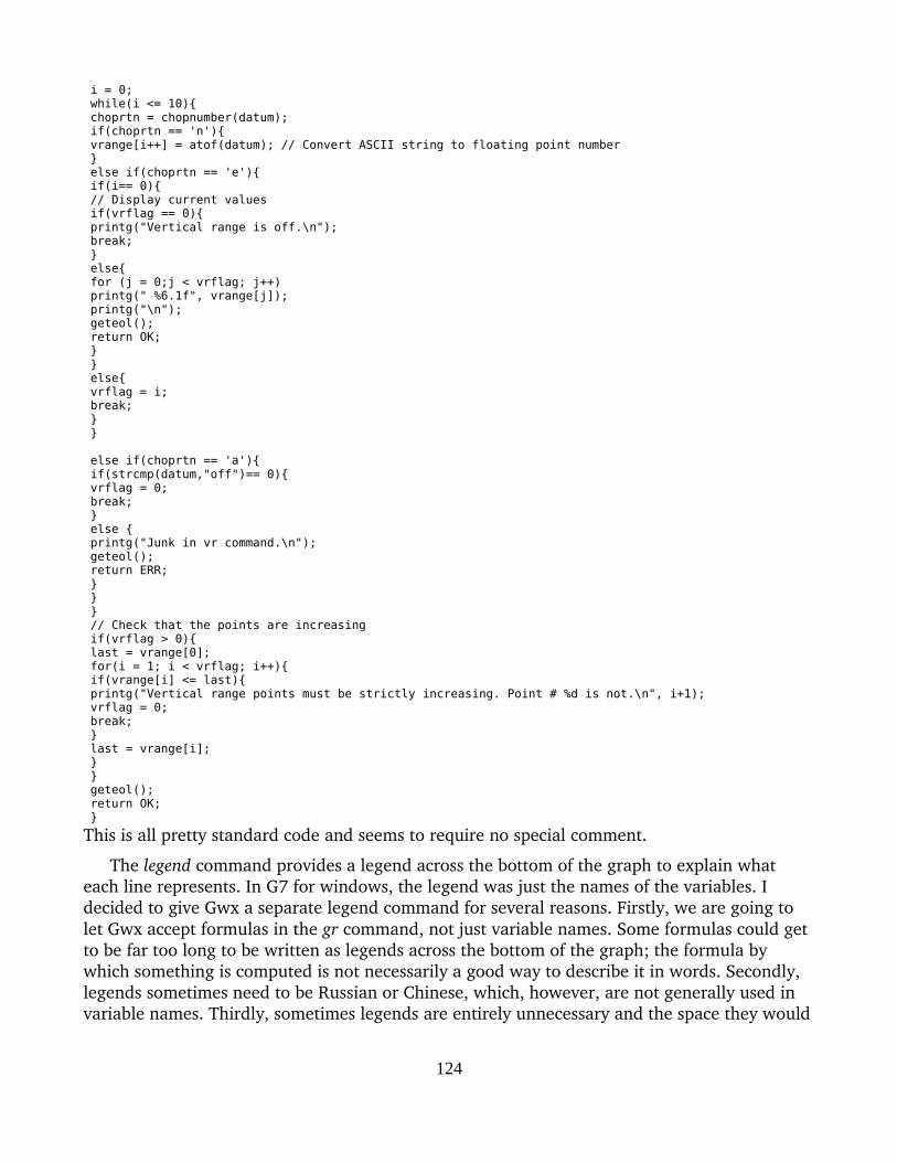
i = 0; while(i <= 10){ choprtn = chopnumber(datum); if(choprtn == 'n'){ vrange[i++] = atof(datum); // Convert ASCII string to floating point number } else if(choprtn == 'e'){ if(i== 0){ // Display current values if(vrflag == 0){ printg("Vertical range is off.\n"); break; } else{ for (j = 0;j < vrflag; j++) printg(" %6.1f", vrange[j]); printg("\n"); geteol(); return OK; } } else{ vrflag = i; break; } }
else if(choprtn == 'a'){ if(strcmp(datum,"off")== 0){ vrflag = 0; break; } else { printg("Junk in vr command.\n"); geteol(); return ERR; } } } // Check that the points are increasing if(vrflag > 0){ last = vrange[0]; for(i = 1; i < vrflag; i++){ if(vrange[i] <= last){ printg("Vertical range points must be strictly increasing. Point # %d is not.\n", i+1); vrflag = 0; break; } last = vrange[i]; } } geteol(); return OK; }
This is all pretty standard code and seems to require no special comment.
The legend command provides a legend across the bottom of the graph to explain what each line represents. In G7 for windows, the legend was just the names of the variables. I decided to give Gwx a separate legend command for several reasons. Firstly, we are going to let Gwx accept formulas in the gr command, not just variable names. Some formulas could get to be far too long to be written as legends across the bottom of the graph; the formula by which something is computed is not necessarily a good way to describe it in words. Secondly, legends sometimes need to be Russian or Chinese, which, however, are not generally used in variable names. Thirdly, sometimes legends are entirely unnecessary and the space they would
124
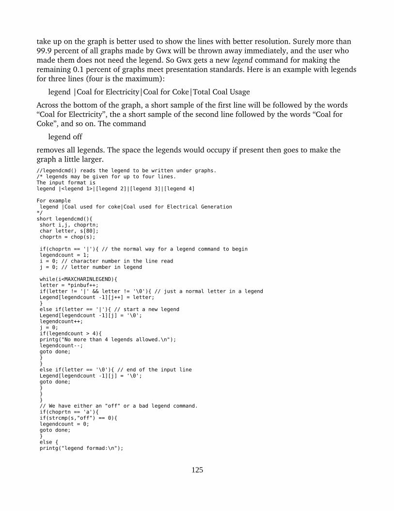
take up on the graph is better used to show the lines with better resolution. Surely more than 99.9 percent of all graphs made by Gwx will be thrown away immediately, and the user who made them does not need the legend. So Gwx gets a new legend command for making the remaining 0.1 percent of graphs meet presentation standards. Here is an example with legendsfor three lines (four is the maximum):
legend |Coal for Electricity|Coal for Coke|Total Coal Usage
Across the bottom of the graph, a short sample of the first line will be followed by the words “Coal for Electricity”, the a short sample of the second line followed by the words “Coal for Coke”, and so on. The command
legend off
removes all legends. The space the legends would occupy if present then goes to make the graph a little larger. //legendcmd() reads the legend to be written under graphs./* legends may be given for up to four lines.The input format islegend |<legend 1>|[legend 2]|[legend 3]|[legend 4]
For example legend |Coal used for coke|Coal used for Electrical Generation*/short legendcmd(){ short i,j, choprtn; char letter, s[80]; choprtn = chop(s);
if(choprtn == '|'){ // the normal way for a legend command to begin legendcount = 1; i = 0; // character number in the line read j = 0; // letter number in legend
while(i<MAXCHARINLEGEND){ letter = *pinbuf++; if(letter != '|' && letter != '\0'){ // just a normal letter in a legend Legend[legendcount -1][j++] = letter; } else if(letter == '|'){ // start a new legend Legend[legendcount -1][j] = '\0'; legendcount++; j = 0; if(legendcount > 4){ printg("No more than 4 legends allowed.\n"); legendcount--; goto done; } } else if(letter == '\0'){ // end of the input line Legend[legendcount -1][j] = '\0'; goto done; } } } // We have either an "off" or a bad legend command. if(choprtn == 'a'){ if(strcmp(s,"off") == 0){ legendcount = 0; goto done; } else { printg("legend formad:\n");
125

printg("legend | <first legend> | <second legend> \n"); printg("up to four legends\n"); printg("or <legend off> to remove all legend."); goto done; } } if(choprtn == 'e'){ for(i = 0;i < legendcount; i++) printg("%s\n",Legend[i]); } done: geteol(); return OK; }
The Plan for the Rest of This Tutorial We will follow the same order of exposition here as we did in Tutorial 3, where we first
wrote Giotto() to draw on any Device Context (dc) and then dealt with with how to get it to write on the screen or to a .PNG file on a disk. Here, however, there is a preliminary step, reading the data – Giotto() needed no data. After writing the program to read and prepare the data, we will write DesCartes() – corresponding to Giotto() – to draw the graph on any Device Context. Only then will we deal with getting the graph on the screen or saved to a file. Our first graph will be very rudimentary with only the title, a box, and in the box the lines of the graph – no scales marked on either axis and no legend. They will come later.
Reading the Data for a GraphAs already hinted, we are going to introduce one generalization of the graph command in
Windows G7. Namely, we will allow in our gr command not only the names of variables already in the data bank but also expressions derived from them by formulas given in the gr command. Thus, in addition to a command like
gr CoalElec, CoalTotal
we will allow
gr CoalTotal, CoalElec + CoalCoke + CoalOthInd
The price of this added versatility is a small inconsistency with G7. Namely, the user of Gwx must separate the variables to be graphed by commas, just as in the r command. In G7, the variable names are separated by spaces.
The graph command will begin very like the r command by creating a matrix, zp, of the series to be graphed. Each series is put into a row of this matrix. We can borrow code from rcmd and simplify it to get the code shown on the Read Data box. The main simplification is that we do not have to deal with the distinction between the first variable and any other, nor do we have to allow for an intercept. Instead of counting the series by the variable niv (Number of Independent Variable's), we will count them with the variable ngrseries. We will put the first series in row 1 of the zp matrix and the first observation of each series will be in column 1 of zp. (That may seem obvious, but it is worth mentioning because C programmers often start in row or column 0. Indeed, in the r command, the dependent variable was in row 0
126

of xp.)
Otherwise, down to the point where we display the matrix for debugging purposes, the two routines are very similar.
In the common.h file, we have already added the following lines which will now be needed:// ngrseries is the number of series to be graphaedGLOBAL unsigned ngrseries;GLOBAL float **zp; //zp is where the data for graphs is storedGLOBAL float GraphRange[2];
We now begin the graph.cpp file as follows:
// graph.cpp contains some graph-related commands
#include "common.h"#include "GraphDialog.h"#include "GiottoDialog.h"
short graphcmd() { short obnoA,obnoB, obnoC; //obno = observation number short nopy; // number of observations per year short grrtn = ERR; // Return value of this routine. // The regression is done between obnoA and obnoB; predicted values are // calculatedout to obnoC
int err; // niv = number of independent variables
// intercept = 0 if there is no intercept; otherwise 1. char s[MAXNAMELENGTH], buf[MAXCHARINTITLE/2];
int i,j,k,obs_total, obs_in_regress;unsigned short MaxCharInTitles = 5*MAXLINE;// titles will become the names of the variables or the formulas for// creating them.char titles[MaxCharInTitles +1], *ptitles[MAXVAR];
/* ptitles[i] points to begining of the title of ith variable *//* The first variable is variable number 0 *///char *cp=0;unsigned size;unsigned char cu;
char *pinbufsave;
GDate fdateAsave,fdateBsave;
grrtn = OK;
obnoA = gdateA.ObNo(); obnoB = gdateB.ObNo(); obnoC = gdateC.ObNo(); nopy = gdateA.freq; obs_total = obnoC - obnoA + 1; obs_in_regress = obnoB -obnoA +1;
// Read the command i = 0; // index of where the character will be put in titles j = 2; // index of where the character is read from in inbuf
while(inbuf[j] == ' ' && j < MAXLINE) j++; //skip spaces
ReadTheCommand: while((cu = inbuf[j++]) != '\n' && cu != '\0' && i < MaxCharInTitles){ if(cu != ' ') titles[i++] = cu; } // Check to see if there is more of the gr command to read on the next line if((cu = titles[i-1]) == ',' || cu == '+' || cu == '-' || cu == '*' || cu == '/' ){ // there is more of this gr command to follow
127

fgets(inbufAsRead,MAXLINE,iin); printg("%s\n",inbufAsRead); k = 0; // Remove the '\n' at the end of s for comparability with what comes from CmdBox. while(inbufAsRead[k] != '\n') k++; inbufAsRead[k] = '\0'; // Perform text substitution textsubstitute(); j = 0; goto ReadTheCommand; } titles[i] = '\0'; pinbuf = inbuf+j-1;
// Count, index and convert titles to strings ngrseries = 0; i = 0; ptitles[0] = &titles[0]; while(i<MaxCharInTitles){ if(titles[i] == '\0') break; if(titles[i] == ','){ titles[i] = '\0'; ngrseries++; ptitles[ngrseries] = &titles[i+1]; } i++; } ngrseries++;
// Create the zp matrix // Prototype:float **matrix(int nrl, int nrh, int ncl, int nch); // nrl = number of first (low) row; nrh = number of last (high) row
zp = matrix(1,ngrseries,1,obs_total); float *series; series = vector(1,nobs_ws);
// Save the current values of pinbuf and fdates pinbufsave = pinbuf; fdateAsave = fdateA; fdateBsave = fdateB;
// Temporarily replace fdates with gdates to trick rhs(). fdateA = gdateA; fdateB = gdateC;
// Read in the variables
for(i = 1; i <= ngrseries; i++){ pinbuf = ptitles[i-1]; // ptitles began at 0. rhs(series); for(j = 1;j <= obs_total;j++) zp[i][j] = series[obnoA+j-1]; }
// Restore pinbuf and fdates pinbuf = pinbufsave; fdateA = fdateAsave; fdateB = fdateBsave; // Debug printg("The matrix of series to be graphed:\n");
for(j = 1;j <= obs_total;j++){ for(i = 1; i <= ngrseries; i++) printg(" %12.4f",zp[i][j]); printg("\n"); } //End Debug
128

At this point, the borrowing from rcmd ceases and we are in new territory. We now have to look over the data doing one of three things depending on the value of vrflag, the vertical range flag, which may have been set using the vrange command. If vrflag is 0, no vertical rangeis specified, and we need to find the highest and lowest values of any variable being graphed. If vrflag is 1, only the lower limit has been set. Usually, that limit will have been set to 0 just tobe sure that 0 is on the graph, so we are going to interpret the “limit” to mean, “Go down at least as far as the limit, but lower if necessary to get all the points.” So in this case, we just start the lower bound off at the specified limit and search for the highest and lowest values in the data, including this lower limit. Finally if vrflag > 1, we don't search at all; rather we trim off any points lying outside the vertical range which has been specified to make the lie on the top or bottom axis. Here is the code: // Find the highest and lowest points or trim to fit the specified vrange. float high, low; if (vrflag == 0 || vrflag == 1){ low = zp[1][1]; if(vrflag == 1) low = vrange[0]; high = low; for(j = 1;j <= obs_total;j++){ for(i = 1; i <= ngrseries; i++){ if (zp[i][j] > high) high = zp[i][j]; else if (zp[i][j] < low) low = zp[i][j]; } } // Fill in values of vrange in the vrflag = 0 or 1 case. // Note that we do NOT change vrflag itself. vrange[0] = low; vrange[1] = low +0.5*(high - low); vrange[2] = high;
} else { // A vertical range with two or more points has been given; clip the data accordingly. low = vrange[0]; high = vrange[vrflag-1]; for(i = 1; i <= ngrseries; i++){ if (zp[i][j] > high) zp[i][j] = high; else if (zp[i][j] < low) zp[i][j] = low; } }
We will put the lowest and highest points in the Global variables GraphRange[0] and GraphRange[1] respectively.
GraphRange[0] = low; GraphRange[1] = high;
The graphcmd() function now concludes with a few statements:
GraphDialog *dlg = new GraphDialog(NULL); dlg->ShowModal();
free_vector(series,1); free_matrix(zp, 1,ngrseries,1);
return grrtn; }
129
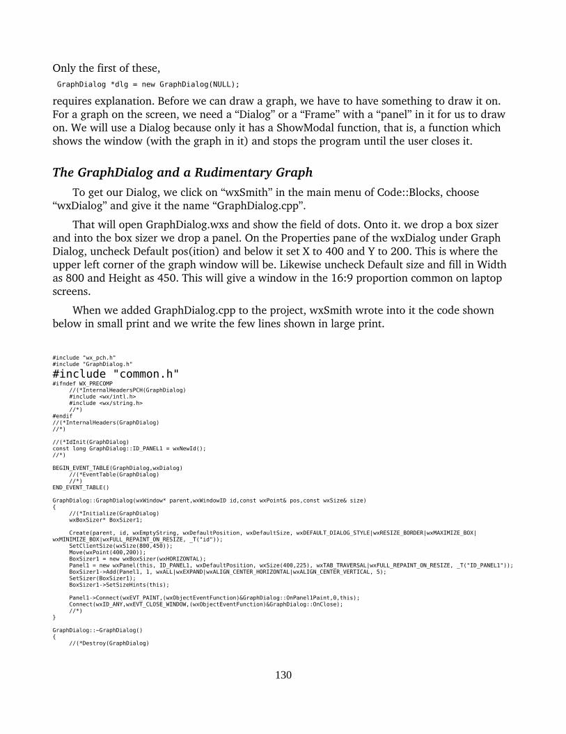
Only the first of these, GraphDialog *dlg = new GraphDialog(NULL);
requires explanation. Before we can draw a graph, we have to have something to draw it on. For a graph on the screen, we need a “Dialog” or a “Frame” with a “panel” in it for us to draw on. We will use a Dialog because only it has a ShowModal function, that is, a function which shows the window (with the graph in it) and stops the program until the user closes it.
The GraphDialog and a Rudimentary Graph To get our Dialog, we click on “wxSmith” in the main menu of Code::Blocks, choose
“wxDialog” and give it the name “GraphDialog.cpp”.
That will open GraphDialog.wxs and show the field of dots. Onto it. we drop a box sizer and into the box sizer we drop a panel. On the Properties pane of the wxDialog under Graph Dialog, uncheck Default pos(ition) and below it set X to 400 and Y to 200. This is where the upper left corner of the graph window will be. Likewise uncheck Default size and fill in Width as 800 and Height as 450. This will give a window in the 16:9 proportion common on laptop screens.
When we added GraphDialog.cpp to the project, wxSmith wrote into it the code shown below in small print and we write the few lines shown in large print.
#include "wx_pch.h"#include "GraphDialog.h"
#include "common.h"#ifndef WX_PRECOMP
//(*InternalHeadersPCH(GraphDialog)#include <wx/intl.h>#include <wx/string.h>//*)
#endif//(*InternalHeaders(GraphDialog)//*)
//(*IdInit(GraphDialog)const long GraphDialog::ID_PANEL1 = wxNewId();//*)
BEGIN_EVENT_TABLE(GraphDialog,wxDialog)//(*EventTable(GraphDialog)//*)
END_EVENT_TABLE()
GraphDialog::GraphDialog(wxWindow* parent,wxWindowID id,const wxPoint& pos,const wxSize& size){
//(*Initialize(GraphDialog)wxBoxSizer* BoxSizer1;
Create(parent, id, wxEmptyString, wxDefaultPosition, wxDefaultSize, wxDEFAULT_DIALOG_STYLE|wxRESIZE_BORDER|wxMAXIMIZE_BOX|wxMINIMIZE_BOX|wxFULL_REPAINT_ON_RESIZE, _T("id"));
SetClientSize(wxSize(800,450));Move(wxPoint(400,200));BoxSizer1 = new wxBoxSizer(wxHORIZONTAL);Panel1 = new wxPanel(this, ID_PANEL1, wxDefaultPosition, wxSize(400,225), wxTAB_TRAVERSAL|wxFULL_REPAINT_ON_RESIZE, _T("ID_PANEL1"));BoxSizer1->Add(Panel1, 1, wxALL|wxEXPAND|wxALIGN_CENTER_HORIZONTAL|wxALIGN_CENTER_VERTICAL, 5);SetSizer(BoxSizer1);BoxSizer1->SetSizeHints(this);
Panel1->Connect(wxEVT_PAINT,(wxObjectEventFunction)&GraphDialog::OnPanel1Paint,0,this);Connect(wxID_ANY,wxEVT_CLOSE_WINDOW,(wxObjectEventFunction)&GraphDialog::OnClose);//*)
}
GraphDialog::~GraphDialog(){
//(*Destroy(GraphDialog)
130

//*)}
void GraphDialog::OnClose(wxCloseEvent& event){
Destroy();}
Click on GraphDialog in the Resources pane and then on the {} symbol in the bar below the Resources pane to bring up event list, then click on the Paint event and provide this code:
void GraphDialog::OnPanel1Paint(wxPaintEvent& event){ wxPaintDC dc( Panel1 ); wxSize sz = GetClientSize();
DesCartes(dc,sz); }
This code first creates a wxPaintDC – the kind of device context used for writing on the screen – called simply dc and sets it to draw on Panel1. Then it finds the current size of dc's client – namely Panel1. Then it calls DesCartes to draw on dc and passes to DesCartes() for his use the present size of Panel1, sz.
We now return to the lines
GraphDialog *dlg = new GraphDialog(NULL);
dlg->ShowModal();
near the end of the graphcmd() function. Their function is clear enough: create an instance of the GraphDialog class and show it modally. But there is a mystery. With Giotto, the same thingwas done by the lines (page 27)
void GwxFrame::OnGiottoBtnClick(wxCommandEvent& event){
GiottoDialog* dlg = new GiottoDialog(this); dlg->ShowModal();
}
so I thought we needed something likeGraphDialog *dlg = new GraphDialog(this);
But the compiler insisted that this was an illegal use of this. On close study, I concluded that the compiler message was correct, but how then was GraphDialog() to be called? After about two days of searching and trying various things without success, I saw an example of creating a Dialog with NULL as the argument. I tried it and it worked! What is called for is a pointer to the parent. When NULL is used, the parent is taken to be the main program. While that is not correct in this case, I have been unable to find a better solution – nor have I had any problems from using NULL.
It is time now to have a look at DesCartes(). But perhaps there is a prior question: Why didwe do the reading of the data and the finding of the low and high values before calling DesCartes()? Why not put all the calculations together in DesCartes()? The answer is rather important: DesCartes() will be called every time the window in which the graph is displayed is resized by the user. Thus, we want to minimize the calculations it must do and limit them to those that depend on the size of the window. With that understanding, the code for a very rudimentary DesCartes() should be clear. It is shown in the box below.
131
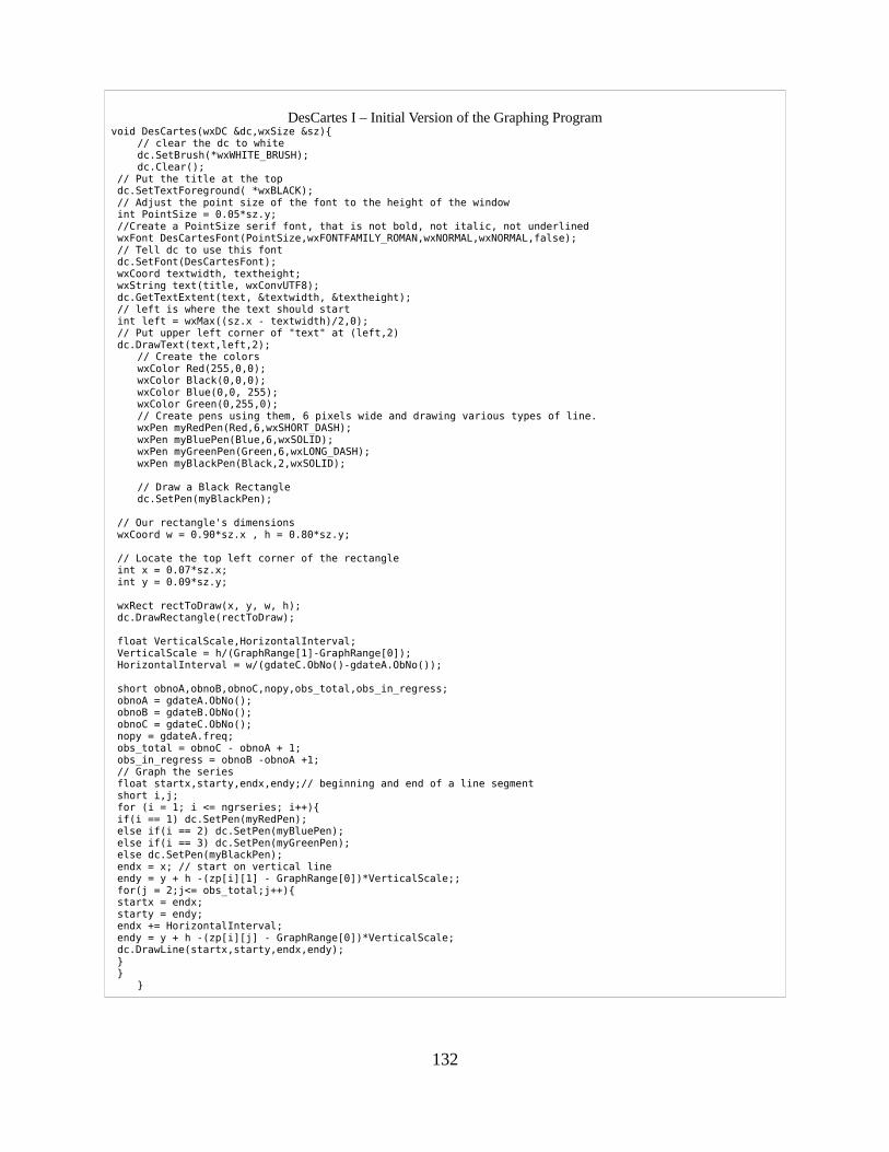
132
DesCartes I – Initial Version of the Graphing Programvoid DesCartes(wxDC &dc,wxSize &sz){
// clear the dc to whitedc.SetBrush(*wxWHITE_BRUSH);dc.Clear();
// Put the title at the top dc.SetTextForeground( *wxBLACK); // Adjust the point size of the font to the height of the window int PointSize = 0.05*sz.y; //Create a PointSize serif font, that is not bold, not italic, not underlined wxFont DesCartesFont(PointSize,wxFONTFAMILY_ROMAN,wxNORMAL,wxNORMAL,false); // Tell dc to use this font dc.SetFont(DesCartesFont); wxCoord textwidth, textheight; wxString text(title, wxConvUTF8); dc.GetTextExtent(text, &textwidth, &textheight); // left is where the text should start int left = wxMax((sz.x - textwidth)/2,0); // Put upper left corner of "text" at (left,2) dc.DrawText(text,left,2);
// Create the colorswxColor Red(255,0,0);wxColor Black(0,0,0);wxColor Blue(0,0, 255);wxColor Green(0,255,0);// Create pens using them, 6 pixels wide and drawing various types of line.wxPen myRedPen(Red,6,wxSHORT_DASH);wxPen myBluePen(Blue,6,wxSOLID);wxPen myGreenPen(Green,6,wxLONG_DASH);wxPen myBlackPen(Black,2,wxSOLID);
// Draw a Black Rectangledc.SetPen(myBlackPen);
// Our rectangle's dimensions wxCoord w = 0.90*sz.x , h = 0.80*sz.y;
// Locate the top left corner of the rectangle int x = 0.07*sz.x; int y = 0.09*sz.y;
wxRect rectToDraw(x, y, w, h); dc.DrawRectangle(rectToDraw);
float VerticalScale,HorizontalInterval; VerticalScale = h/(GraphRange[1]-GraphRange[0]); HorizontalInterval = w/(gdateC.ObNo()-gdateA.ObNo());
short obnoA,obnoB,obnoC,nopy,obs_total,obs_in_regress; obnoA = gdateA.ObNo(); obnoB = gdateB.ObNo(); obnoC = gdateC.ObNo(); nopy = gdateA.freq; obs_total = obnoC - obnoA + 1; obs_in_regress = obnoB -obnoA +1; // Graph the series float startx,starty,endx,endy;// beginning and end of a line segment short i,j; for (i = 1; i <= ngrseries; i++){ if(i == 1) dc.SetPen(myRedPen); else if(i == 2) dc.SetPen(myBluePen); else if(i == 3) dc.SetPen(myGreenPen); else dc.SetPen(myBlackPen); endx = x; // start on vertical line endy = y + h -(zp[i][1] - GraphRange[0])*VerticalScale;; for(j = 2;j<= obs_total;j++){ startx = endx; starty = endy; endx += HorizontalInterval; endy = y + h -(zp[i][j] - GraphRange[0])*VerticalScale; dc.DrawLine(startx,starty,endx,endy); } }
}

Here is what the graph of the fit of our regression looks like. As I said before, it is pretty rudimentary, it lacks scales and a legend, but it is a beginning.
Incidentally, however, I have tried it with both Chinese and Russian titles, and it works fine.
A DesCartes with Labeling of the Vertical and Horizontal AxesRené would not approve, I am sure, of any graphing routine bearing his name that did not
label both the vertical and horizontal axes, so here is a more evolved version which provides that labeling. Exactly 17 of its 350+ lines are concerned with drawing the lines of the graph. Everything else is about putting the titles, scales, and legend on the graph. So be prepared for some minutiae.
Drawing the black rectangle into which the graph will be drawn is the first order of business and requires knowing the heights of the title, subtitle, legend, and horizontal axis labels and the widths of the vertical axis labels. Its size and position will then be fundamental for the rest of the graph. In what follows, the code itself is in a sansserif monospaced font, andI may break in here and there with further comment is this serif proportional font.
void DesCartes(wxDC &dc,wxSize &sz){ int i;
// clear the dc to whitedc.SetBrush(*wxWHITE_BRUSH);dc.Clear();
// Put the title at the top dc.SetTextForeground( *wxBLACK);
Precisely what the relation is between point size of the font and how much space the text takesup on the screen I do not know. It is clearly important to relate the point size to the size of the client window, but the relation, the .05 in the formula below, was just determined by what looked nice.
// Adjust the point size of the font for the title to the height of the window
133
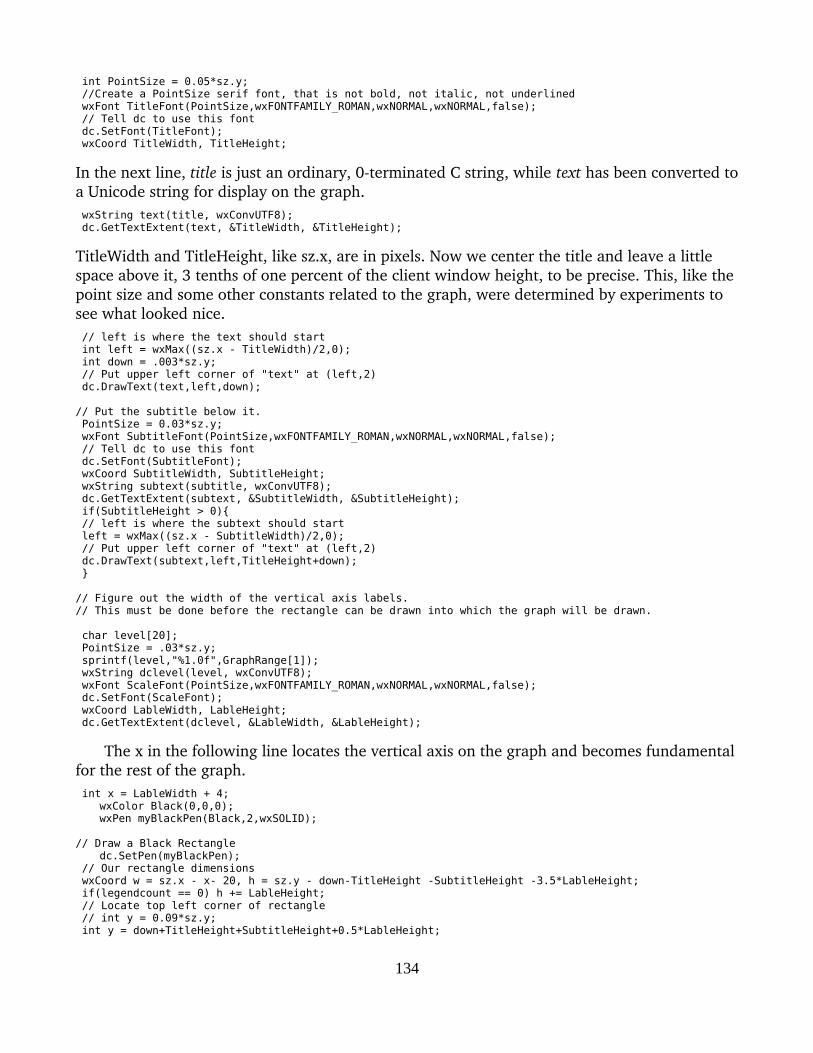
int PointSize = 0.05*sz.y; //Create a PointSize serif font, that is not bold, not italic, not underlined wxFont TitleFont(PointSize,wxFONTFAMILY_ROMAN,wxNORMAL,wxNORMAL,false); // Tell dc to use this font dc.SetFont(TitleFont); wxCoord TitleWidth, TitleHeight;
In the next line, title is just an ordinary, 0terminated C string, while text has been converted toa Unicode string for display on the graph. wxString text(title, wxConvUTF8); dc.GetTextExtent(text, &TitleWidth, &TitleHeight);
TitleWidth and TitleHeight, like sz.x, are in pixels. Now we center the title and leave a little space above it, 3 tenths of one percent of the client window height, to be precise. This, like thepoint size and some other constants related to the graph, were determined by experiments to see what looked nice. // left is where the text should start int left = wxMax((sz.x - TitleWidth)/2,0); int down = .003*sz.y; // Put upper left corner of "text" at (left,2) dc.DrawText(text,left,down);
// Put the subtitle below it. PointSize = 0.03*sz.y; wxFont SubtitleFont(PointSize,wxFONTFAMILY_ROMAN,wxNORMAL,wxNORMAL,false); // Tell dc to use this font dc.SetFont(SubtitleFont); wxCoord SubtitleWidth, SubtitleHeight; wxString subtext(subtitle, wxConvUTF8); dc.GetTextExtent(subtext, &SubtitleWidth, &SubtitleHeight); if(SubtitleHeight > 0){ // left is where the subtext should start left = wxMax((sz.x - SubtitleWidth)/2,0); // Put upper left corner of "text" at (left,2) dc.DrawText(subtext,left,TitleHeight+down); }
// Figure out the width of the vertical axis labels.// This must be done before the rectangle can be drawn into which the graph will be drawn.
char level[20]; PointSize = .03*sz.y; sprintf(level,"%1.0f",GraphRange[1]); wxString dclevel(level, wxConvUTF8); wxFont ScaleFont(PointSize,wxFONTFAMILY_ROMAN,wxNORMAL,wxNORMAL,false); dc.SetFont(ScaleFont); wxCoord LableWidth, LableHeight; dc.GetTextExtent(dclevel, &LableWidth, &LableHeight);
The x in the following line locates the vertical axis on the graph and becomes fundamentalfor the rest of the graph. int x = LableWidth + 4;
wxColor Black(0,0,0);wxPen myBlackPen(Black,2,wxSOLID);
// Draw a Black Rectangledc.SetPen(myBlackPen);
// Our rectangle dimensions wxCoord w = sz.x - x- 20, h = sz.y - down-TitleHeight -SubtitleHeight -3.5*LableHeight; if(legendcount == 0) h += LableHeight; // Locate top left corner of rectangle // int y = 0.09*sz.y; int y = down+TitleHeight+SubtitleHeight+0.5*LableHeight;
134

wxRect rectToDraw(x, y, w, h); dc.DrawRectangle(rectToDraw);
// Label and mark the vertical axis int NumberOfVerticalIntervals; NumberOfVerticalIntervals = vrflag -1; //Label at least the top, bottom, and midpoint if(vrflag <= 1) NumberOfVerticalIntervals = 2;
float VerticalScale = h/(GraphRange[1] - GraphRange[0]);
float startx,starty,endx,endy,rightStartx, rightEndx;// beginning and end of a line segment
for(i = 0;i <= NumberOfVerticalIntervals; i++){ sprintf(level,"%1.0f",vrange[i]); wxString dclevel(level, wxConvUTF8); dc.DrawText(dclevel,2,y - 0.5*LableHeight + h - VerticalScale*(vrange[i] - GraphRange[0])); // Mark the scale startx = x; endx = x+.02*sz.x + 1; rightStartx = x+w - .02*sz.x -1; rightEndx = x + w;
starty = y+h -VerticalScale*(vrange[i] - GraphRange[0]); endy = starty; if(i > 0 && i < NumberOfVerticalIntervals){ dc.DrawLine(startx,starty,endx,endy); dc.DrawLine(rightStartx,starty,rightEndx,endy); } }
// Create the colorswxColor Red(255,0,0);wxColor Blue(0,0, 255);wxColor Green(0,255,0);// Create pens using them, 3 pixels wide and drawing various styles of line.wxPen myRedPen(Red,3,wxSHORT_DASH);wxPen myBluePen(Blue,3,wxSOLID);wxPen myGreenPen(Green,3,wxLONG_DASH);
double HorizontalInterval;
In the next line, note the cast of w to a double. This w was declared as a wxCoordinate, which seem to mean integer. Without the cast, the righthand side would be an integer dividedby an interger, and the remainder would be thrown away before the quotient was saved as a double.The result would be that the intervals do not fill the whole of the horizontal axis. With the cast, it works fine. (The need for the cast was learned the hard way.) HorizontalInterval = double(w)/(gdateC.ObNo()-gdateA.ObNo()+1);
short obnoA,obnoB,obnoC,nopy,obs_total,obs_in_regress; obnoA = gdateA.ObNo(); obnoB = gdateB.ObNo(); obnoC = gdateC.ObNo(); nopy = gdateA.freq; obs_total = obnoC - obnoA + 1; obs_in_regress = obnoB -obnoA +1;
// In order to write the legend, we need to know the height of the dates, // which will be above the legend. PointSize = 0.03*sz.y; //Create a PointSize serif font, that is not bold, not italic, not underlined wxFont DatesFont(PointSize,wxFONTFAMILY_ROMAN,wxNORMAL,wxNORMAL,false); // Tell dc to use this font dc.SetFont(DatesFont); wxCoord DateWidth, DateHeight;
135

char date[20]; sprintf(date,"%4d",gdateA.year); wxString year(date, wxConvUTF8); dc.GetTextExtent(year, &DateWidth, &DateHeight);
// Establish Variables for writing the legends wxCoord LegendWidth, LegendHeight; LegendWidth = 0; PointSize = 0.03*sz.y; wxFont LegendFont(PointSize,wxFONTFAMILY_ROMAN,wxNORMAL,wxNORMAL,false); wxString LegendText; char thislegend[MAXCHARINLEGEND];
// Graph the series short j,legendstart; legendstart = 2; for (i = 1; i <= ngrseries; i++){ if(i == 1) dc.SetPen(myRedPen); else if(i == 2) dc.SetPen(myBluePen); else if(i == 3) dc.SetPen(myGreenPen); else dc.SetPen(myBlackPen); endx = x + 0.5*HorizontalInterval; // start in middle of first interval endy = y + h -(zp[i][1] - GraphRange[0])*VerticalScale;; for(j = 2;j<= obs_total;j++){ startx = endx; starty = endy; endx += HorizontalInterval; endy = y + h -(zp[i][j] - GraphRange[0])*VerticalScale; dc.DrawLine(startx,starty,endx,endy); }
// Add Legend at bottom if(legendcount > 0){ // Tell dc to use the Legend font dc.SetFont(LegendFont); for(j = 0; j < MAXCHARINLEGEND; j++){ thislegend[j] = Legend[i-1][j]; if(thislegend[j] == '\0') break; } wxString LegendText(thislegend, wxConvUTF8); dc.GetTextExtent(LegendText, &LegendWidth, &LegendHeight); if(LegendHeight > 0){ startx = legendstart; endx = startx + .10*sz.x; starty = y+h + 0.01*sz.y + 1.1*DateHeight + .7*LegendHeight -3; endy = starty; dc.DrawLine(startx,starty,endx,endy); legendstart = endx+0.02*sz.x; dc.DrawText(LegendText,endx +0.02*sz.x,starty-.7*LegendHeight+3); legendstart += LegendWidth + .04*sz.x; } } }
This first marking just makes a short mark at the end of every interval. It is general and easy. // Mark horizontal scale dc.SetPen(myBlackPen); starty = y+h -1; // the horizontal axis endy = starty - .015*sz.y; startx = x; for (j = 2; j <= obs_total;j++){ startx = x + (j-1)*HorizontalInterval; endx = startx; dc.DrawLine(startx,starty,endx,endy); }
dc.SetFont(DatesFont);
136

wxCoord textwidth, textheight;
Marking more heavily the annual divisions of quarterly and monthly data, and fiveyear divisions of annual data is more tricky and must be done with separate code for the three periodicities.
// With quarterly data, mark year divisions // and label horizontal axis. short first_year, last_year; first_year = gdateA.year; last_year = gdateC.year;
if(gdateA.freq == 4){ starty -= 1; // improves the look of the graph wxPen myWidePen(Black,3,wxSOLID); dc.SetPen(myWidePen); endy = starty - 0.03*sz.y; i = 0; while (i+4 < obs_total){ startx = (i+5 - gdateA.period)*HorizontalInterval +x; endx = startx; dc.DrawLine(startx,starty,endx,endy); i += 4; }
// *** Write the years on the scale *** // Tell dc to use the DatesFont defined above.
int range = last_year - first_year; for (i = first_year; i <= last_year; i++){ sprintf(date,"%4d",i); wxString year(date, wxConvUTF8); dc.GetTextExtent(year, &textwidth, &textheight); // left is where the text should start left = x + 4.*(i - first_year)*HorizontalInterval +
2.*HorizontalInterval - 0.5*textwidth; // Put upper left corner of "text" at (left,) if(range <= 10) dc.DrawText(year,left,y+h + 0.01*sz.y); else if (i%5 == 0) dc.DrawText(year,left,y+h + 0.01*sz.y); } } // End of marking the horizontal axis with quarterly data
// With monthly data, mark year divisions // and label horizontal axis. if(gdateA.freq == 12){ starty -= 1; // improves the look of the graph wxPen myWidePen(Black,3,wxSOLID); dc.SetPen(myWidePen); endy = starty - 0.03*sz.y; i = 0;
i = gdateA.period; i = 13 - i; // How far to first December while (i <= obs_total){ startx = i*HorizontalInterval +x; endx = startx; dc.DrawLine(startx,starty,endx,endy); i += 12; } // Write years if(gdateA.period != 1) first_year++; if(gdateC.period != 12) last_year--; i = 13 - gdateA.period; int skip = i*HorizontalInterval;
for (i = first_year; i <= last_year; i++){ sprintf(date,"%4d",i);
137
wxString year(date, wxConvUTF8); dc.GetTextExtent(year, &textwidth, &textheight); // left is where the text should start left = x + skip + 12.*(i - first_year)*HorizontalInterval +
6.*HorizontalInterval - 0.5*textwidth; // Put upper left corner of "text" at (left,) dc.DrawText(year,left,y+h + 0.01*sz.y); } }
// With annual data, mark 5 year divisions and write year labels every five years if(gdateA.freq == 1){ starty -= 1; // improves the look of the graph wxPen myWidePen(Black,3,wxSOLID); dc.SetPen(myWidePen); endy = starty - 0.03*sz.y;
i = gdateA.year % 5; i = 5 -i; // i is how many intervals we must move to the right to get to the // beginning of a five-year period. while (i < obs_total){ startx = i*HorizontalInterval +x; endx = startx; dc.DrawLine(startx,starty,endx,endy); i += 5; }
// *** Write the years on the scale *** // Tell dc to use the DatesFont defined above. dc.SetFont(DatesFont); wxCoord textwidth, textheight;
short first_year, last_year; first_year = gdateA.year; last_year = gdateC.year;
int range = last_year - first_year; for (i = first_year; i <= last_year; i++){ sprintf(date,"%4d",i); wxString year(date, wxConvUTF8); dc.GetTextExtent(year, &textwidth, &textheight); // left is where the text should start left = x + (i - first_year +.5)*HorizontalInterval - 0.5*textwidth; // Put upper left corner of "text" at (left,) if(range <= 10) dc.DrawText(year,left,y+h + 0.01*sz.y); else if (i%5 == 0) dc.DrawText(year,left,y+h + 0.01*sz.y); } } // end of marking and labeling the horizontal axis with annual data
return;}
Well, that was a lot of work and we still haven't marked the points with +, * and the like. wxWidgets is better than Borland Builder at distinguishing between solid, dashed, and dotted lines, so the point markers are not so essential. Eventually, of course, we want to add selectionby the user of colors, marks and line types – including bars. But that can wait. Right now we still need to be able to save our graph.
The gname Command.If we are going to save a graph, we need a file to save it in. Originally, I just wrote all
graphs to the same file, each erasing any previous one. But of course that soon had to be
138
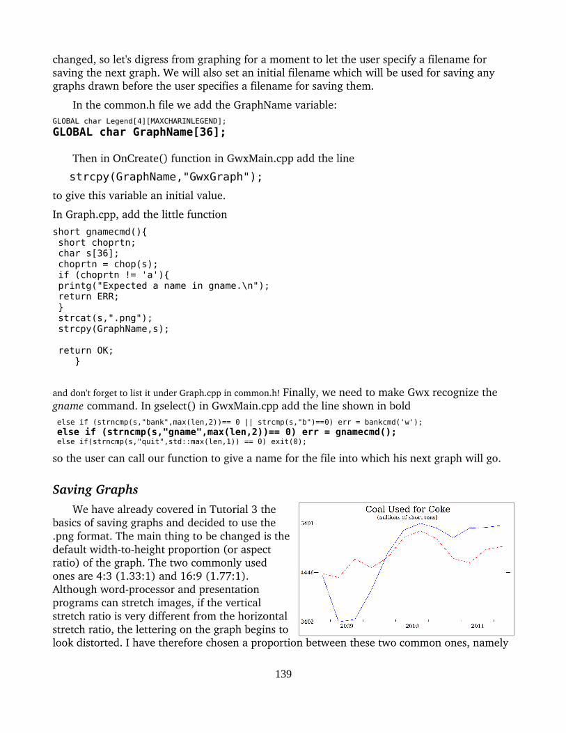
changed, so let's digress from graphing for a moment to let the user specify a filename for saving the next graph. We will also set an initial filename which will be used for saving any graphs drawn before the user specifies a filename for saving them.
In the common.h file we add the GraphName variable:GLOBAL char Legend[4][MAXCHARINLEGEND];
GLOBAL char GraphName[36];
Then in OnCreate() function in GwxMain.cpp add the line
strcpy(GraphName,"GwxGraph");
to give this variable an initial value.
In Graph.cpp, add the little function
short gnamecmd(){ short choprtn; char s[36]; choprtn = chop(s); if (choprtn != 'a'){ printg("Expected a name in gname.\n"); return ERR; } strcat(s,".png"); strcpy(GraphName,s);
return OK; }
and don't forget to list it under Graph.cpp in common.h! Finally, we need to make Gwx recognize the gname command. In gselect() in GwxMain.cpp add the line shown in bold else if (strncmp(s,"bank",max(len,2))== 0 || strcmp(s,"b")==0) err = bankcmd('w'); else if (strncmp(s,"gname",max(len,2))== 0) err = gnamecmd(); else if(strncmp(s,"quit",std::max(len,1)) == 0) exit(0);
so the user can call our function to give a name for the file into which his next graph will go.
Saving GraphsWe have already covered in Tutorial 3 the
basics of saving graphs and decided to use the.png format. The main thing to be changed is thedefault widthtoheight proportion (or aspectratio) of the graph. The two commonly usedones are 4:3 (1.33:1) and 16:9 (1.77:1).Although wordprocessor and presentationprograms can stretch images, if the verticalstretch ratio is very different from the horizontalstretch ratio, the lettering on the graph begins tolook distorted. I have therefore chosen a proportion between these two common ones, namely
139
1.618, which happens to give the golden rectangle. It is the outer border which has the golden proportion. This border, however, is not drawn by Gwx since it is easily supplied by the word processor if desired, while getting rid of it if undesired is troublesome.
here is the preliminary version of graph saving. ... GraphDialog *dlg = new GraphDialog(NULL); dlg->ShowModal();
// Save the graph /* To save our drawing to a file, we first create a bitmap, then
a memory DC, then hand the bitmap to the memory DC to use aspaper to draw on, then have DesCartes draw on it, then free thebitmap from the DC, then make it write itself as a .png file.
*/// Create a bitmap 2000 pixels wide and 1236 pixels high, approximate golden rectangle.// Call it "paper" because we will write on it. wxBitmap *paper = new wxBitmap( 2000,1236);
// Create a memory Device Context wxMemoryDC memDC;
// Tell memDC to write on “paper”. memDC.SelectObject( *paper );// Set up sz to give DesCartes the size of paper. wxSize sz; sz.x = 2000; sz.y = 1236;
// Call Descartes to draw our picture on memDC DesCartes(memDC,sz);
// Tell memDC to write on a fake bitmap;// this frees up "paper" so that it can write itself to a file. memDC.SelectObject( wxNullBitmap );
// Put the contents of "paper” into a png file.
wxString wxGraphName = wxString::FromAscii(GraphName); paper->SaveFile(wxGraphName,wxBITMAP_TYPE_PNG,(wxPalette*)NULL); //paper->SaveFile(wxGraphName, wxBITMAP_TYPE_JPEG, (wxPalette*)NULL );
free_vector(series,1);g free_matrix(zp, 1,ngrseries,1); delete paper; return grrtn; }
I have emphasized the line
wxString wxGraphName = wxString::FromAscii(GraphName);because it cost me hours of agony. In the next line, wxGraphName must be in Unicode. The _T() macro that had worked when given a quoted string back in Tutorial 3 utterly failed when given the name of a variable containing a C string. It would not compile and stopped with the error marker in a system routine I had not written. I knew I had to get the GraphName variable into Unicode, but how? After hours of search on the Internet and reading many documents that were no doubt clear to their authors but not to me, I stumbled on the FromAscii() function in wxWidgets. It seemed worth trying, and – lo – it worked! I suppose I should go back and change Giotto in Tutorial 3, but have not done so.
At this point, we have a fairly adequate graph command.
140

Tutorial 13. Assigned Data Banks IOne of G's most useful features is its ability to draw data series from previously prepared
data banks, such as the quarterly or annual national accounts of various countries. Another useof this feature is to assign as different banks the results of running a forecasting model under alternative assumptions and to use G's graphing ability to show the differences in the forecasts.
In this tutorial, we will add the ability to assign and draw data from a number of banks all having the standard form of the workspace bank we have already introduced. G7 has two more types of data banks called compressed banks and hashed banks. The first of these, the compressed bank, may require as little as half as much storage space for series drawn from printed sources as does the standard bank. The hashed bank can hold millions of series insteadof the few thousand of the standard bank. These bank types were worth developing back in thedays when RAM was tight and diskspace scarce. Today, their development is far less pressing and may never be undertaken.
Gwx will, however, be able to handle VAM files, data banks holding time series of vectors and matrices – from whence comes the VAM name.
Since the code for handling data banks is pure C++ with no reference to wxWidgets, we could just dump it in here exactly as it stands in G7. In reading over that code, however, I find that it has become hard to follow. I believe that a newcomer to the innards of G will welcome a gradual, tutorial introduction to this rather complicated subject.
I cannot, however, pass up this opportunity to relate what is now an amusing incident in the evolution of the G program and The Craft of Economic Modeling. Some years ago, a representative of a textbook publishing company visited my office, saw a photocopy version of The Craft that I was then using, and asked to consider it for publication. I gave him a copy, anda week or so later heard back that the firm's outside reviewer liked the content and the writingbut needed to work with the software to make a final recommendation. A week or so later, I received a letter informing me that the reviewer found the software unacceptable because it used a data bank. The data bank required some 250 kilobytes of space on the hard disk, and the reviewer was sure that few public universities would be able to afford computers with that much storage. At the time, one could not buy a computer with a hard disk of less than 20 megabytes, and bigger ones were commonplace. I laughed and threw the letter in the trash. A few minutes later, a graduate assistant, Amy Carr, came in, and I fished the letter out and showed it to her. “That's so stupid!” she exclaimed, “You have to write back to him.” I did, pointing out a few facts about computers. But the editor replied that he was sure the reviewer was right and that, were he free to reveal the man's name, I would surely agree, so authoritative was he. It was a good lesson in how ignorant “authorities” can be. Actually, I am grateful to the reviewer for saving me from entanglement with a commercial publisher who could have impeded the further development of The Craft.
Assigning and Referencing BanksGwx, like G7, is to have the possibility of assigning and drawing data from up to 22
141
different data banks in addition to the workspace bank. These banks are to be designated by the letter a, b, c, …, v. (We stop before w because 22 has always been more than enough banks and we wish to avoid any confusion which w might cause since it is used in some contexts to designate the workspace bank.) To specify that a variable in a Gwx command is to come from a particular bank, we precede the variable name by the bank's letter followed by a period, for example d.savings. A variable name not preceded by a single letter and period will be searched for in the workspace bank and bank a if one has been assigned. (G7 has an option to go on searching through all the assigned banks. The option is very easy to write and use, butI regard it as foolhardy; those who wrote and use it think they are smart enough to never get tricked by it. I am sure that I am not.)
The handling of data banks can be – and originally was – programmed without using C++devices such as classes and virtual functions. However, it also lends itself to programming using these constructs and was reprogrammed in the current version of G7 using them. We will follow this structure but try, of course, to explain the ideas as we progress.
The DataBank ClassWe begin with a class called DataBank from which we will derive classes called Gbank and,
later, VamFile. The DataBank class will provide space to hold some variables which any bank will require, such as the number of series in the bank, nseries. These variables will be declared as “protected”, that is to say, as accessible to functions in this class and in classes derived from it but not in other parts of the program. It also provides “public” functions for reporting the values of these variables to any part of the Gwx program that needs to know them. Thus, any part of Gwx can learn the number of series in a particular bank, but only code in the DataBankclass or classes derived from it can change the value of nseries.
Some of these functions in the DataBank class are declared as virtual, for example:
virtual unsigned short GetBaseYr(void){return jahra;}
A virtual function may be redefined in some – but not necessarily all – derived classes. However, the function that gets a series from a bank, getser(), is so different for each type of bank that there is no reasonable default definition for it. Therefore, no definition of it is given in the DataBank class and it becomes a pure virtual function that must be defined in derived classes. It is declared like this:
virtual short getser(char *nam,float *f,short SeriesLength=-1)=0;
The =0; at the end of the line is a C++ convention to mark it as a pure virtual function.
Because the DataBank class has a pure virtual function, it is called an abstract class, and noinstance of it can be declared. That is, we cannot write
DataBank mybank;
What good then is an abstract class? In the first place, we can save some coding by
142
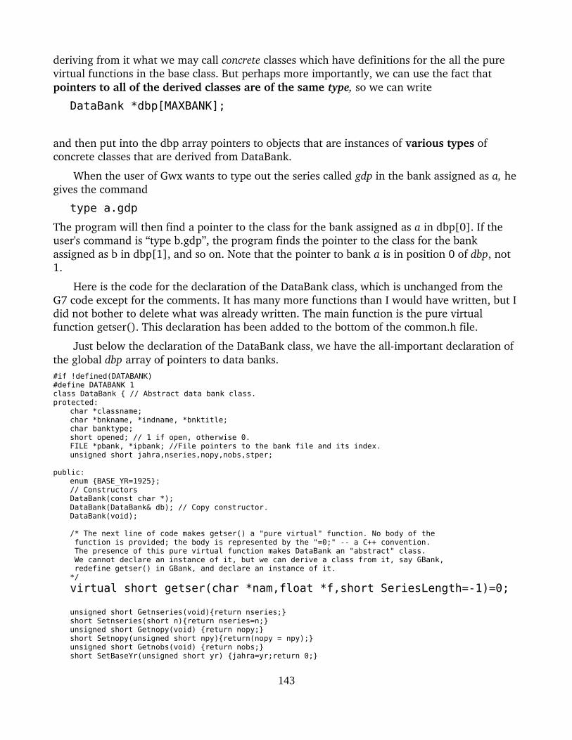
deriving from it what we may call concrete classes which have definitions for the all the pure virtual functions in the base class. But perhaps more importantly, we can use the fact that pointers to all of the derived classes are of the same type, so we can write
DataBank *dbp[MAXBANK];
and then put into the dbp array pointers to objects that are instances of various types of concrete classes that are derived from DataBank.
When the user of Gwx wants to type out the series called gdp in the bank assigned as a, he gives the command
type a.gdp
The program will then find a pointer to the class for the bank assigned as a in dbp[0]. If the user's command is “type b.gdp”, the program finds the pointer to the class for the bank assigned as b in dbp[1], and so on. Note that the pointer to bank a is in position 0 of dbp, not 1.
Here is the code for the declaration of the DataBank class, which is unchanged from the G7 code except for the comments. It has many more functions than I would have written, but Idid not bother to delete what was already written. The main function is the pure virtual function getser(). This declaration has been added to the bottom of the common.h file.
Just below the declaration of the DataBank class, we have the allimportant declaration of the global dbp array of pointers to data banks. #if !defined(DATABANK)#define DATABANK 1class DataBank { // Abstract data bank class.protected:
char *classname;char *bnkname, *indname, *bnktitle;char banktype;short opened; // 1 if open, otherwise 0.FILE *pbank, *ipbank; //File pointers to the bank file and its index.unsigned short jahra,nseries,nopy,nobs,stper;
public:enum {BASE_YR=1925};// ConstructorsDataBank(const char *);DataBank(DataBank& db); // Copy constructor.DataBank(void);
/* The next line of code makes getser() a "pure virtual" function. No body of the function is provided; the body is represented by the "=0;" -- a C++ convention. The presence of this pure virtual function makes DataBank an "abstract" class. We cannot declare an instance of it, but we can derive a class from it, say GBank, redefine getser() in GBank, and declare an instance of it. */
virtual short getser(char *nam,float *f,short SeriesLength=-1)=0;
unsigned short Getnseries(void){return nseries;} short Setnseries(short n){return nseries=n;}unsigned short Getnopy(void) {return nopy;}short Setnopy(unsigned short npy){return(nopy = npy);}unsigned short Getnobs(void) {return nobs;}short SetBaseYr(unsigned short yr) {jahra=yr;return 0;}
143

short Setstper(short n){stper=n;return 0;}short Getstper(void) {return stper;}
// some cheap inline definitions of virtual functions that may or may not get improved.virtual unsigned short GetBaseYr(void){return jahra;}virtual short showcmd(char *s, FILE* iin){return(1);}
virtual float **Getnmvec(void){return(0);} virtual short loadcmd(char *s,char view, float line){return(0);}
virtual short storecmd(){return(0);} virtual long findname(char *name){return(0);} virtual long Getnrows(int i){return(0);}// for finding rows of Vam element i virtual long Getncols(int i){return(0);} virtual char GetElementType(int i){return(0);} // for Vam Files
virtual short ListNames()=0; // Display the names of series in this bank.virtual short Announce(short bankno=0);
short IsOpen(void){return (opened==1); }short IsErr(void) {return (opened==-1); }char *Getclassname(void){return classname;}char *Getbnkname(void) {return bnkname;}char *Getindname(void){return indname;}char *Getbnktitle(void){return bnktitle;}virtual char *Setbnktitle(const char *s);char Getbanktype(void){return banktype;}// This is an abstract base class, and therefore *must* have a virtual destructor:virtual ~DataBank(){}
};
GLOBAL DataBank *dbp[MAXBANK]; // array of DataBank pointers.#endif
Derivation of the GBank Class from the Abstract DataBank ClassThe class for each type of databank will be derived from this abstract class. Here is the declaration of the class for the workspacetype bank, which – in conformity with the practice inG7 – we will call the GBank class, while the other three classes will be CBank, HBank, and Vbank. This declaration is in the file GBank.h, which starts off with the declaration of the bankHeader struct.// GBANK.H -- Class declarations for a standard G data bank.#if !defined(GBANK_H)#define GBANK_H 1
// If we don't use this check on BNKHEADER, fixbank and gbank cause multiple declarations.#if !defined(BNKHEADER)#define BNKHEADER 1#include "common.h"
struct bnkHeader {short jahra; //base year of all series in the bankshort stper; //starting period within the base year, usually 1short nobs; // number of observations for which space is reserved.char bnktitle[MAXBANKTITLE];};
#endif
Now we need to derive the GBank class from the more general abstract DataBank class. Butfirst, a confession. All of this code is borrowed with little or no alteration from G7 for Windows. In that program, the workspace is a bank of the GBank class. We already have our workspace for Gwx and do not need – for the moment – to replace it. We will use banks of the
144

the GBank type only as an assigned bank, a, b, c, etc. Now one of the fundamental rules of both G7 and Gwx is that the program cannot modify an assigned bank. Were it possible to do so, in a class with many students using the same assigned bank havoc would soon result. Even if only one or two people are using a bank, we want to make sure that changing data in it is a very conscious process, not something likely to happen by accident. Therefore, the assigned banks are assigned as read only. Only the workspace is assigned for both reading and writing. But since G7 for Windows uses the same class for both the workspace and assigned banks, its DataBank class has some routines for modifying the series in the data bank. We may later wantto make it possible to assign an existing GBank as the workspace, so I have left the code for these bankmodifying functions even though it is not at this point possible to access them. To tell you which functions are used in Gwx at this point, I have marked them with // ** Gwx // in the following declaration of the GBank class. It is found in GBank.h, and here is what it looks like:
class GBank : public DataBank {// GBank: Object to handle transactions with simple GBank file.
protected:// ncin is number of characters in names.unsigned int ncin;char *names;unsigned short *indx;
char status;
public://using namespace std;enum {NCMAX=65535, NSMAX=17241};
char cnpy; // number of observations per year; 13 for daily data; changed by each getser call.// constructorsGBank(void); // default constructor// copy constructor:GBank(GBank&);
// The following constructor defaults to "Read", but can also be "ReadWrite"GBank(const char *rootname, const char *status="Read",
short BaseYr=1965, short nobserv=200, short stper=1, short silent=0); // ** Gwx //virtual char *Setbnktitle(const char *s);// destructor ~GBank(); // ** Gwx //
short AssignBank(const char *rootname); // Assign an already constructed bank.// Reading and writing of the index file.short windex(void);short rindex(void); // ** Gwx //
// Put and get series int addser(char *nam, float *f, char wrindex_flag='y', short SeriesLength=-1);
virtual short getser(char *nam, float *f, short SeriesLength=-1); // ** Gwx //// Display the names of the series in the bank.virtual short ListNames(); // ** Gwx //short findname(char *gname); // ** Gwx //
char* GetName(int loc,char *gname); short flush(void);
int delser(char *gname); short rename(char *oldname, char *newname); short DelRen(char Status, char*oldname, char *newname=NULL); // inline functions
short Getnobs(void) {return nobs;}; unsigned short Getnseries(void){return nseries;}; };
145

Functions for the GBank ClassNow we need the code to define the functions of the class. It is in GBank.cpp; the portions
presently relevant to Gwx are shown below. #include <algorithm>#include "common.h"#include "GBank.h"using namespace std; // for max and min/*==========================================================================*//* The GBank constructor.
This multifunction constructor has been borrowed unchanged from G7, and is more general than is initially needed for Gwx because we will keep our workspace constructor. The first argument gives the root (excluding the .bnk) of the filename of the bank to be opened. The second argument, FileStatus, tells how the bank is to be opened. If FileStatus == "Read", the program will open an existing bank for reading only. This is the default, as specified in the function's declaration in GBank.h:
GBank(const char *rootname, const char *status="Read", short BaseYr=1965, short nobserv=200, short stper=1, short silent=0);
So if called with just the first argument, the constructor will open an existing bank for reading only. That is the only use we will initially make of it in Gwx. = = = = A few comments not immediately relevant for Gwx:
For a new file, use FileStatus="New".For a file being assigned as a G workspace bank, use FileStatus = "ReadWrite".nobserv = maximum number of observationsst = period of first observation in base year, normally 1silent = 1 shuts off some debugging print
*/GBank::GBank(const char *rootname, const char *FileStatus, short BaseYr, short nobserv, short st, short silent) {
short err,j; int i; long posit; char fname[120],FileOptions[10]; char tmps[120]; bnkHeader Hdr; char status;
if(strcmp(FileStatus,"Read")==0){ // For normal opening of an assigned bank. strcpy(FileOptions,"rb"); // rb = open an existing binary file for reading only. status='r'; }
else if(strcmp(FileStatus,"New")==0){ // For creating an empty workspace bank. strcpy(FileOptions,"w+b"); // w+b = Create a binary file for both reading and writing. jahra = Hdr.jahra = BaseYr; nobs = Hdr.nobs = nobserv; stper = Hdr.stper = st; status='n'; strcpy(Hdr.bnktitle,"Untitled"); }
else if(strcmp(FileStatus,"ReadWrite")==0){ // Open an existing bank as the workspace bank. strcpy(FileOptions,"r+b"); // r+b = open an existing binary file for reading and writing. status='+'; }
bnktitle=0; classname=0; bnkname=0; indname=0; nseries=0; pbank=0;
146
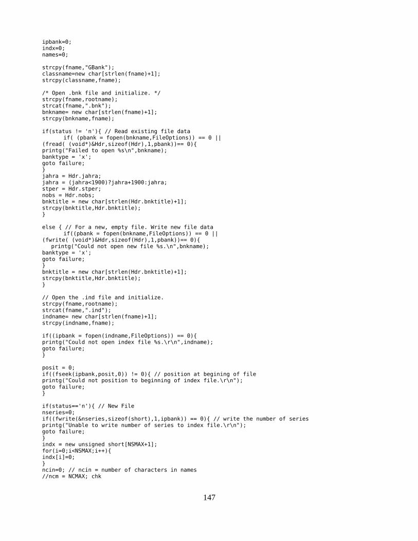
ipbank=0; indx=0; names=0;
strcpy(fname,"GBank"); classname=new char[strlen(fname)+1]; strcpy(classname,fname);
/* Open .bnk file and initialize. */ strcpy(fname,rootname); strcat(fname,".bnk"); bnkname= new char[strlen(fname)+1]; strcpy(bnkname,fname);
if(status != 'n'){ // Read existing file dataif( (pbank = fopen(bnkname,FileOptions)) == 0 ||
(fread( (void*)&Hdr,sizeof(Hdr),1,pbank))== 0){ printg("Failed to open %s\n",bnkname); banktype = 'x'; goto failure; } jahra = Hdr.jahra; jahra = (jahra<1900)?jahra+1900:jahra; stper = Hdr.stper; nobs = Hdr.nobs; bnktitle = new char[strlen(Hdr.bnktitle)+1]; strcpy(bnktitle,Hdr.bnktitle); }
else { // For a new, empty file. Write new file dataif((pbank = fopen(bnkname,FileOptions)) == 0 ||
(fwrite( (void*)&Hdr,sizeof(Hdr),1,pbank))== 0){ printg("Could not open new file %s.\n",bnkname); banktype = 'x'; goto failure; } bnktitle = new char[strlen(Hdr.bnktitle)+1]; strcpy(bnktitle,Hdr.bnktitle); }
// Open the .ind file and initialize. strcpy(fname,rootname); strcat(fname,".ind"); indname= new char[strlen(fname)+1]; strcpy(indname,fname);
if((ipbank = fopen(indname,FileOptions)) == 0){ printg("Could not open index file %s.\r\n",indname); goto failure; }
posit = 0; if((fseek(ipbank,posit,0)) != 0){ // position at begining of file printg("Could not position to beginning of index file.\r\n"); goto failure; }
if(status=='n'){ // New File nseries=0; if((fwrite(&nseries,sizeof(short),1,ipbank)) == 0){ // write the number of series printg("Unable to write number of series to index file.\r\n"); goto failure; } indx = new unsigned short[NSMAX+1]; for(i=0;i<NSMAX;i++){ indx[i]=0; } ncin=0; // ncin = number of characters in names //ncm = NCMAX; chk
147

names = new char[NCMAX]; strcpy(names,""); } else{ // Existing file if((fread(&nseries,sizeof(short),1,ipbank)) == 0){ // read the number of series printg("Could not read number of series in existing bank.\n\r"); goto failure; } if(status=='+'){ // indx = new unsigned short[NSMAX]; } else{ indx = new unsigned short[nseries+1]; }
// Read the pointer but allow and empty bank to be opened with error. if(nseries!=0 && (fread(indx,sizeof(short),nseries+1,ipbank)) == 0){ printg("Could not read the pointer (indx) to names.\r\n"); goto failure; }
if(indx[nseries] > 65534 ){ printg("Overflow in Gbank constructor.\r\n"); goto failure; }
ncin = indx[nseries]+1; if(status=='+') names = new char[NCMAX]; else names = new char[ncin];
if(nseries != 0 && (fread(names,1,ncin,ipbank)) == 0){ // read the names printg("Could not read the names.\n\r"); goto failure; } }
banktype = 'w'; goto success; failure: opened = -1; if(classname){ delete[] classname; classname=0; } if(bnkname){ delete[] bnkname; bnkname=0; } if(indname){ delete[] indname; indname=0; } if(indx){ delete[] indx; indx=0; } if(names){ delete[] names; names=0; } return;
success: opened = 1; return; }
148

/*==========================================================================*/// The GBank destructor.// free up memory allocated in constructor and close data files.GBank::~GBank(){if(status=='w')
windex(); // make sure to write index.if(classname){
delete[] classname;classname=0;}
if(bnkname){delete[] bnkname;bnkname=0;}
if(bnktitle){delete[] bnktitle;bnktitle=0;}
if(indname){delete[] indname;indname=0;}
if(indx){delete[] indx;indx=0;}
if(names){delete[] names;names=0;}
if(pbank){ fclose(pbank); pbank = NULL; }if(ipbank){ fclose(ipbank); ipbank = NULL; }}
/*==========================================================================*/// Read the index file.short GBank::rindex(void) { // Read index from index file.long posit,err;
posit = 0;if((fseek(ipbank,posit,0)) != 0){ /* posit at begin of file */
printg("Could not position to read index file.\n");return(ERR);}
if((fread(&nseries,2,1,ipbank)) == 0){ /* read the number of series */printg("Could not read nseries from index file.\n");return(ERR);}
if((fread(indx,2,nseries+1,ipbank)) == 0){ /* read the pointer */printg("Could not read the pointers in the index file.\n");return(ERR);}
ncin = indx[nseries] + 1;if((fread(names,1,ncin,ipbank)) == 0){ /* read the names */
printg("Could not read the names in the index file.\n");return(ERR);}
printg("G bank index read.\n");return(0);}
149

/* findname -- finds position of given name in GBank names array. */short GBank::findname(char *gname){ unsigned long j; short i;
for(i=0;i<nseries;i++){ j = indx[i];
if(strcmp(gname,&names[j])==0){ return(i); } }printg("%s not found.\n",gname);return(-1);}
/*==========================================================================*/// getser – get a series from a Gbank. // Lines up the series with the workspace, // It is a member of the GBank class, and so knows protected information in that class.
short GBank::getser(char *nam, float *ss, short SeriesLength){
int err,i,gap;// ,max_obs; unsigned long position; short NameNumber; int shift; float val; char cnpy, test; char lagtext[MAXNAMELENGTH];
GDate StartDate;
// A series name will often not be found. The user may have forgotten the name, // or mistyped it, or the series may be in some other bank.
// The following call to findname() goes to the findname() that is part of the GBank class. // The value returned is the sequence number of the name in the bank.
if((NameNumber = findname(nam)) == -1) goto notfound;
/* In the following formula: position is the number of bytes preceding the series we are looking for. sizeof(bnkHeader) is the number of bytes in the header with the title; NameNumber is the number of bytes consumed in giving each preceding series its frequency; temp * (long)nobs * sizeof(float) is the number of bytes in the preceeding series. */
position = (long)NameNumber * (long)nobs * sizeof(float) + NameNumber + sizeof(bnkHeader);
if((err = fseek(pbank,position,0)) == ERR){ printg("Cannot position to read location of %s in GBank.\n",nam); return(ERR); }
if((err=fread(&cnpy,1,1,pbank))==0 ) { printg("Cannot read frequncy of %s.\n",nam); return(ERR); }
nopy=cnpy;
if(SeriesLength==-1) SeriesLength=nobs; // check if this argument was given. for( i=0;i<SeriesLength;i++)
ss[i] = 0;
if((err=fread((void*)ss,sizeof(float),SeriesLength,pbank))==0) { printg("Cannot read %s.\n",nam); return(ERR);
150

}
// Check for a lag, indicated by a number in brackets, like this: gdp{3].// First, steal a look ahead without increasing pinbuf. test = *pinbuf; if(test == '['){//found a lag pinbuf++; //increment pinbuf to get past the [ short choprtn = chop(lagtext); if(choprtn != 'n'){ // read the lag printg("Expected a number for the lag on %s\n", nam); geteol(); return ERR; } short lag = atoi(lagtext); // Shift the series forward; note that we start at the top for(i = SeriesLength; i >= lag; i--) ss[i] = ss[i-lag];
// Fill in the unknown values at the beginning with MISSING for(i = lag-1; i >= 0; i--) ss[i] = MISSING; choprtn = chop(lagtext); // Get past the closing ] if(choprtn != ']'){ printg("Expected a ] after the lag on %s.\n",nam); geteol(); return ERR; } }
//Does this series need to be shifted to line up properly with the workspace?if(nopy == 0)return 0; //Don't shift variables with 0 freq.
StartDate.set((short)jahra, (char)stper, 1, (char)nopy);shift = StartDate.ObNo();if(shift < 0){ // Series begins before workspace //Prevent buffer overrun when shift<0 && SeriesLength==NOMAX
int maximum = min(SeriesLength - shift, NOMAX + shift);for(i = 0; i < maximum; i++)
ss[i] = ss[i-shift];}
if(shift > 0){ // Series begins after workspacefor(i = SeriesLength+shift-1; i >= shift; i--)
ss[i] = ss[i-shift];for(i = 0; i < shift; i++)
ss[i] = MISSING;}
return nopy;
notfound: return(ERR); }
short GBank::ListNames(){ // Display the names of series in this bank. printg("ListNames is not yet written\n"); }
Most of this code is familiar from the getseries() function for dealing with the workspace bank. There is, however, one important addition to deal with, namely the fact the starting dateof the assigned bank may be different from that of the workspace bank. Since the data series read from the assigned bank may be combined with series in the workspace, it must be shifted forward of backward to line up with the workspace. The code that does that alignment follows the comment:
151

//Does this series need to be shifted to line up properly with the workspace?This code makes good use of the GDate class. It simply converts the starting date of the
assigned bank to a GDate and then finds the observation number (relative to the workspace) ofthat date. If that observation number – called shift in the code – is negative, then a series read from the assigned bank begins before the workspace and observations must be moved nearer the beginning of the ss array. Conversely, if shift is positive, observations must be moved farther from the beginning of the vector. Notice in the code that in this case the i subscript starts at its highest value and moves down, as indicated by the i in the for loop.
With the GBank class ready for use, we now need to add a command to Gwx to open a bank file, assign it to one of positions a through v, and create an instance of the of the GBank class to handle it. We also need to modify the getseries() function called by the type, graph, f, rand other commands so that if the series is not in the workspace, the program will look in the assigned bank. As we assign databanks, each bank will be represented in the computer's memory by an instance of its class, whether it be of the workspace type (w) or the compressed type (c), the hashed type (h), or the vam type (v). If the user of Gwx assigns a workspace type bank as bank a, an instance of the GBank class is created.
If the user works a while and than decides to assign a different bank as a, we should deletethe first instance of the GBank class before creating an instance of the class of the new bank. Otherwise, we may suffer serious memory leaks. We will in due course write a routine which we can call to delete whatever kind of bank is in a given position, a, b, c, etc. But to write that routine, we must first have written the destuctors for all the bank types, just as we have done for the GBank class. To allow ourselves to proceed linearly, step by step, writing and testing the constructors and accessing routines for each type of bank, we are going to sidestep the deletion issue by simply not allowing a bank position – a, b, c, etc. – to be reassigned. We will come back and fix that problem later.
To see whether a position already has a bank assigned to it, we check the corresponding value in dbp. If that value is NULL, no bank has been assigned to the position; otherwise, one has been assigned. To be sure that this check will work, we must assign a value of NULL to all elements of dbp when the program starts. So we open GwxMain.cpp(), and modify the OnCreate() routine as shown by the three lines in large type below: void GwxFrame::OnCreate(wxWindowCreateEvent& event){
short i; printout[0] = '\0';
for (i =0;i < MAXBANK; i++)
dbp[i] = NULL; // Just for testing substitutes strcpy(substitutes[0],"Aaa"); strcpy(substitutes[1],"Bbb"); keyboard = 'y'; MaxRegVar = MAXVAR; MaxRegObs = NOMAX; vrflag = 0; }
152
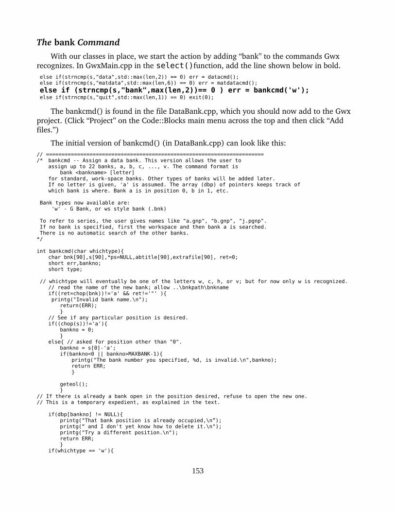
The bank CommandWith our classes in place, we start the action by adding “bank” to the commands Gwx
recognizes. In GwxMain.cpp in the select()function, add the line shown below in bold. else if(strncmp(s,"data",std::max(len,2)) == 0) err = datacmd(); else if(strncmp(s,"matdata",std::max(len,6)) == 0) err = matdatacmd();
else if (strncmp(s,"bank",max(len,2))== 0 ) err = bankcmd('w'); else if(strncmp(s,"quit",std::max(len,1)) == 0) exit(0);
The bankcmd() is found in the file DataBank.cpp, which you should now add to the Gwx project. (Click “Project” on the Code::Blocks main menu across the top and then click “Add files.”)
The initial version of bankcmd() (in DataBank.cpp) can look like this:// ======================================================================/* bankcmd -- Assign a data bank. This version allows the user to assign up to 22 banks, a, b, c, ..., v. The command format is bank <bankname> [letter] for standard, work-space banks. Other types of banks will be added later.
If no letter is given, 'a' is assumed. The array (dbp) of pointers keeps track ofwhich bank is where. Bank a is in position 0, b in 1, etc.
Bank types now available are: 'w' - G Bank, or ws style bank (.bnk) To refer to series, the user gives names like "a.gnp", "b.gnp", "j.pgnp". If no bank is specified, first the workspace and then bank a is searched. There is no automatic search of the other banks.*/
int bankcmd(char whichtype){char bnk[90],s[90],*ps=NULL,abtitle[90],extrafile[90], ret=0;short err,bankno;short type;
// whichtype will eventually be one of the letters w, c, h, or v; but for now only w is recognized.// read the name of the new bank; allow ..\bnkpath\bnknameif((ret=chop(bnk))!='a' && ret!='"' ){ printg("Invalid bank name.\n");
return(ERR);}
// See if any particular position is desired.if((chop(s))!='a'){
bankno = 0;}
else{ // asked for position other than "0".bankno = s[0]-'a';if(bankno<0 || bankno>MAXBANK-1){
printg("The bank number you specified, %d, is invalid.\n",bankno);return ERR;}
geteol();}
// If there is already a bank open in the position desired, refuse to open the new one.// This is a temporary expedient, as explained in the text.
if(dbp[bankno] != NULL){ printg("That bank position is already occupied,\n”);
printg(“ and I don't yet know how to delete it.\n"); printg("Try a different position.\n");
return ERR; }
if(whichtype == 'w'){
153

dbp[bankno] = new GBank(bnk);// If the user gave a bank that does not exist, the attempt to open will have failed.// We check for that possibility with a call to IsOpen(),// an inline function defined in common.h. if(dbp[bankno]->IsOpen() ){ //Was the attempt to open successful?
NumAssigned++;BankType[bankno] = whichtype;dbp[bankno]->Announce(bankno); //Announce to the user that that the bank has been assigned.return(OK);}
else{printg("Unable to open %s as assigned bank %c. Continuing.\n",
bnk,'a'+bankno);printg(“There may have been memory leakage in the failed attempt.\n”;BankType[bankno] = ' ';dbp[bankno] = NULL;
return(ERR);}
/* Activate this code in Tutorial 19else if(whichtype == 'v') {
vf = new VamFile(bnk); dbp[bankno] = vf; }*/
}
Also in bankcmd.cpp is the Announce() function which was used when opening the file and creation of the instance of the class was successful.short DataBank::Announce(short bankno){ // Inform the user what bank has been assigned and its properties. printg("You have just assigned a bank with these properties:\n"); printg("Bank title: %s \n",bnktitle); printg("Base year %d \n",jahra); printg("Number of observations %d \n",nobs); printg("Number of series %d \n",nseries);
return 0; }
The IsOpen() function was used above in bankcmd() to see whether the bank was successfully opened. It is an example of a device which frequently has to be used in C++. It would seem natural to have the constructor for DataBank return OK if the construction was successful and otherwise ERR. But somewhat strangely and unfortunately, in C++ a constructor cannot have a return value. So instead the constructor sets the value of some variable to record whether or not it was successful and provides a function to query the value of that variable. Our constructor of an instance of the DataBank class uses such a device. If the constructor is successful, the value of the variable opened is set to 1; otherwise it is set to zero. The little inline function IsOpen defined in the declaration of DataBank in the common.h
bool IsOpen(void){return (opened==1); }
returns the truth value (true or false) of the statement “the value of opened is 1.” In other words, it returns true if the constructor was successful. Notice that if the constructor is ultimately unsuccessful, it carefully releases any memory it may have claimed.
Extending getseries() to Use the Assigned Banks.When a type, graph, f, or r command needs a series, it calls the getseries() function which is
154
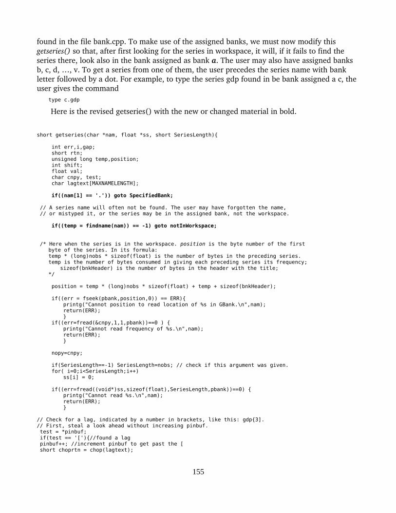
found in the file bank.cpp. To make use of the assigned banks, we must now modify this getseries() so that, after first looking for the series in workspace, it will, if it fails to find the series there, look also in the bank assigned as bank a. The user may also have assigned banks b, c, d, …, v. To get a series from one of them, the user precedes the series name with bank letter followed by a dot. For example, to type the series gdp found in be bank assigned a c, the user gives the command
type c.gdp
Here is the revised getseries() with the new or changed material in bold.
short getseries(char *nam, float *ss, short SeriesLength){
int err,i,gap; short rtn; unsigned long temp,position; int shift; float val; char cnpy, test; char lagtext[MAXNAMELENGTH];
if((nam[1] == '.')) goto SpecifiedBank;
// A series name will often not be found. The user may have forgotten the name, // or mistyped it, or the series may be in the assigned bank, not the workspace.
if((temp = findname(nam)) == -1) goto notInWorkspace;
/* Here when the series is in the workspace. position is the byte number of the firstbyte of the series. In its formula:
temp * (long)nobs * sizeof(float) is the number of bytes in the preceding series. temp is the number of bytes consumed in giving each preceding series its frequency;
sizeof(bnkHeader) is the number of bytes in the header with the title; */
position = temp * (long)nobs * sizeof(float) + temp + sizeof(bnkHeader);
if((err = fseek(pbank,position,0)) == ERR){ printg("Cannot position to read location of %s in GBank.\n",nam); return(ERR); }
if((err=fread(&cnpy,1,1,pbank))==0 ) { printg("Cannot read frequency of %s.\n",nam); return(ERR); }
nopy=cnpy;
if(SeriesLength==-1) SeriesLength=nobs; // check if this argument was given. for( i=0;i<SeriesLength;i++)
ss[i] = 0;
if((err=fread((void*)ss,sizeof(float),SeriesLength,pbank))==0) { printg("Cannot read %s.\n",nam); return(ERR); }
// Check for a lag, indicated by a number in brackets, like this: gdp{3].// First, steal a look ahead without increasing pinbuf. test = *pinbuf; if(test == '['){//found a lag pinbuf++; //increment pinbuf to get past the [ short choprtn = chop(lagtext);
155

if(choprtn != 'n'){ // read the lag printg("Expected a number for the lag on %s\n", nam); geteol(); return ERR; } short lag = atoi(lagtext); // Shift the series forward; note that we start at the top for(i = SeriesLength; i >= lag; i--) ss[i] = ss[i-lag]; // Fill in the unknown values at the beginning with MISSING for(i = lag-1; i >= 0; i--) ss[i] = MISSING; choprtn = chop(lagtext); // Get past the closing ] if(choprtn != ']'){ printg("Expected a ] after the lag on %s.\n",nam); geteol(); return ERR; } }
return nopy;
notInWorkspace: if (dbp[0] != NULL){
rtn = dbp[0]->getser(nam,ss); return(rtn); }
return(ERR);
SpecifiedBank: short BankNumber; BankNumber = nam[0] - 'a'; if (BankNumber < 0 || BankNumber > 22){
printg("Bank letter must be between a and v.\n"); return (ERR); }
if(dbp[BankNumber]== NULL){ printg("No bank has been assigned to that letter.\n"); return (ERR); } printg("BankNumber %d series name %s \n",BankNumber,&nam[2]); rtn = dbp[BankNumber]->getser(&nam[2],ss); return(rtn); }
Modification of rhs()The rhs(float *z) function, it will be recalled, computes the values of expressions on the
right side of an f command, or in a graph command, or on the right side of an r command. It makes use of two vectors, x, and y, in the course of computing the final value of z, the returned value. In the original version of rhs(), x and y were dimensioned 0 to nobws (number of observations in the workspace). Each series used in the expression to be evaluated was read directly into the y vector. That will no longer work once it becomes possible to read data from an assigned bank which may have series longer than the workspace. Consequently, we must introduce a new array, which we will call series, of size NOMAX – the maximum number of observations which Gwx can handle in any one series. We then pass series, not y, to getseries(), which will read the data from either the workspace or an assigned bank into series and, in the case of data from an assigned bank, shift the data forward or backward to line up with the workspace. Then we copy from series to y the portion of the data required by the current values of the fdates. The x and y vectors can be given smaller dimensions, since they
156
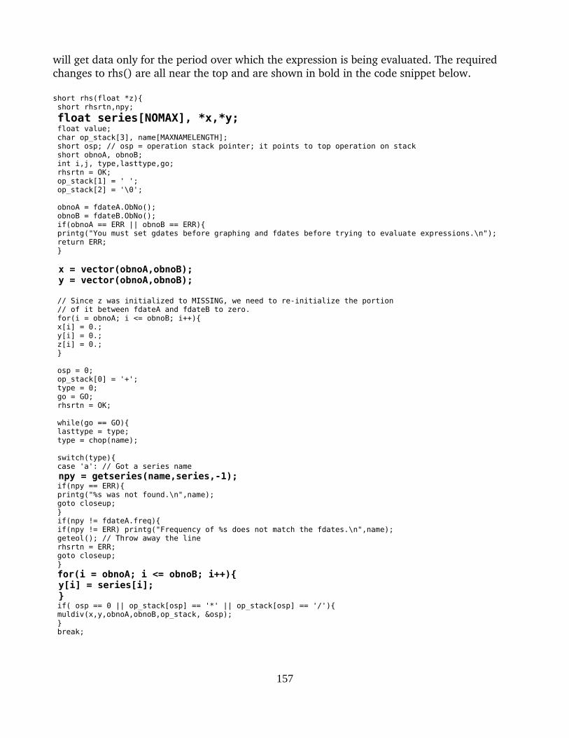
will get data only for the period over which the expression is being evaluated. The required changes to rhs() are all near the top and are shown in bold in the code snippet below.
short rhs(float *z){ short rhsrtn,npy;
float series[NOMAX], *x,*y; float value; char op_stack[3], name[MAXNAMELENGTH]; short osp; // osp = operation stack pointer; it points to top operation on stack short obnoA, obnoB; int i,j, type,lasttype,go; rhsrtn = OK; op_stack[1] = ' '; op_stack[2] = '\0';
obnoA = fdateA.ObNo(); obnoB = fdateB.ObNo(); if(obnoA == ERR || obnoB == ERR){ printg("You must set gdates before graphing and fdates before trying to evaluate expressions.\n"); return ERR; }
x = vector(obnoA,obnoB); y = vector(obnoA,obnoB);
// Since z was initialized to MISSING, we need to re-initialize the portion // of it between fdateA and fdateB to zero. for(i = obnoA; i <= obnoB; i++){ x[i] = 0.; y[i] = 0.; z[i] = 0.; }
osp = 0; op_stack[0] = '+'; type = 0; go = GO; rhsrtn = OK;
while(go == GO){ lasttype = type; type = chop(name);
switch(type){ case 'a': // Got a series name npy = getseries(name,series,-1); if(npy == ERR){ printg("%s was not found.\n",name); goto closeup; } if(npy != fdateA.freq){ if(npy != ERR) printg("Frequency of %s does not match the fdates.\n",name); geteol(); // Throw away the line rhsrtn = ERR; goto closeup; } for(i = obnoA; i <= obnoB; i++){ y[i] = series[i]; } if( osp == 0 || op_stack[osp] == '*' || op_stack[osp] == '/'){ muldiv(x,y,obnoA,obnoB,op_stack, &osp); } break;
157

TestWe will test our code by assigning the U.S. quarterly income and product account bank,
quip, which was made by G7 under Windows, typing and graphing series and running regressions with it. To be sure that the code for lining up series from the assigned bank with the workspace is working correctly, we will set our workspace to begin in 1975, while quip begins in 1955. Here are the results of a somewhat silly regression of residential construction, vfrR, on real GDP, gdpR.
: Residential Construction
SEE = 65.2 RSQ = 0.766 RHO = 0.975 DW = 0.050
Variable name RegCoef Mexval Elas NorRes Means
1 intercept -191.23344 14.1 -0.45 4.28 1.00
2 gdpR 0.06636 106.9 1.45 1.00 9340.24
Not only was the data successfully drawn from quip, but it was correctly lined up with the workspace as is easily seen by anyone familiar with the volatile vfrR series.
SummaryThis has been a long and somewhat complicated chapter. Let us try to summarize it. First,
beginning on page 142, we wrote the abstract DataBank class from which classes for each typeof bank will be derived. Immediately following its definition, on page 143, we declared dbp[], the 22element array of pointers to assigned banks a through v. Then, starting on page 144, wederived the GBank class from the DataBank class and wrote (or borrowed) its member functions, especially the rindex() – read index – function on page 149. We could then, on page153, introduce the bank command into the list of those recognized by Gwx. We then wrote thecode for the command. On page 154, we extended getseries() so that if a series is not in the
158

workspace but bank a is assigned, it will look there also. At the same time, we made getseries() recognize a form such as d.gdp, as meaning that it should get the gdp series from the bank assigned as d. We made some small changes in rhs() so that graph, f, and r commands (which call rhs() ) can work with series drawn from banks not having the same starting and ending dates as does the workspace. Then, to test our code, we assigned a data bank made on G7 under Windows and successfully drew and worked with data from it. In retrospect, it all seems clear and logical, but I can assure you that it was not so – at least not tome – at the outset.
159

Tutorial 14. Saving Results from Regression: The save and catchCommands; gr * and #
The results of a regression often need to be incoorporated into an econonometric model orincluded in a book or paper. The
save <filename>
command saves the results the following regression (or regressions) in the named file until thecommand
save off
is encountered. The results are saved in a format that is easily used by G's sister program build to construct a model that can be run to simulate the behavior of the economy. The form in which the results are saved, however, is not well adapted for reading by humans. So there is another command
catch <filename>
which “catches” what goes on the screen in the named file. It can then be brought into a wordprocessor such as LibreOffice Writer and used to show the results of a regression.
The basic mechanics of the two commands is similar. Into common.h we put two new variables, saving and catching, and file pointers, fpsave and fpcatch, for the files into which the regression results will be written the two lineslike this:GLOBAL short NumAssigned; // Number of assigned banks.
GLOBAL char saving, catching; GLOBAL FILE *fpsave,*fpcatch;
// prototypes // In GwxMain void printg(char *fmt, ...);
We will set saving equal to y when saving is on and to n when it is off, and likewise for catching. They need to be initialized to n when the program starts, so in GwxMain.cpp in GwxFrame::OnCreate() we add the two lines shown in larger type below:void GwxFrame::OnCreate(wxWindowCreateEvent& event){ short i; printout[0] = '\0'; for (i =0;i < MAXBANK; i++) dbp[i] = NULL; // Just for testing substitutes strcpy(substitutes[0],"Aaa"); strcpy(substitutes[1],"Bbb"); keyboard = 'y'; MaxRegVar = MAXVAR; MaxRegObs = NOMAX; vrflag = 0;
saving = 'n';
160

catching = 'n'; }
Next we need to make the program recognize the save and catch commands, so in GwxMain.cpp in the gselect() function we add the second and third lines shown below (in the larger, bold font):
else if(strcmp(s,"r") == 0) err = rcmd();
else if (strncmp(s,"save",std::max(len,3)) == 0) err = savecmd();
else if (strncmp(s,"catch",std::max(len,3)) == 0) err = catchcmd();
And finally we put the save and closely parallel catch commands themselves at the end of rcmd.cpp, like this:int savecmd(){
char s[80], ret;
if((ret=chop(s)) != 'a' ){printg("The save command must be followed by a file name or the word \"off\".\n");return(ERR);}
// See whether all we need do is to turn off savingif(strcmp(s,"off") == 0){
if(saving == 'n'){printg("Saving is not on.\n");}
if(saving == 'y'){fclose(fpsave);
fpsave = 0; saving = 'n';
}return(OK);}
else{ // Open the save file (if not already open).if(saving == 'y'){
printg("Saving is already on.\n");printg("Use \"save off\" before starting a new save file.\n");return(OK);}
if((fpsave = fopen(s,"w+"))==0){printg("Could not open %s.\n",s);return(ERR);}
saving = 'y';}
return(OK);}
int catchcmd(){char s[80], ret;
if((ret=chop(s)) != 'a' ){printg("The catch command must be followed by a file name or the word \"off\".\n");return(ERR);}
// See whether all we need do is to turn off catchingif(strcmp(s,"off") == 0){
if(catching == 'n'){
161
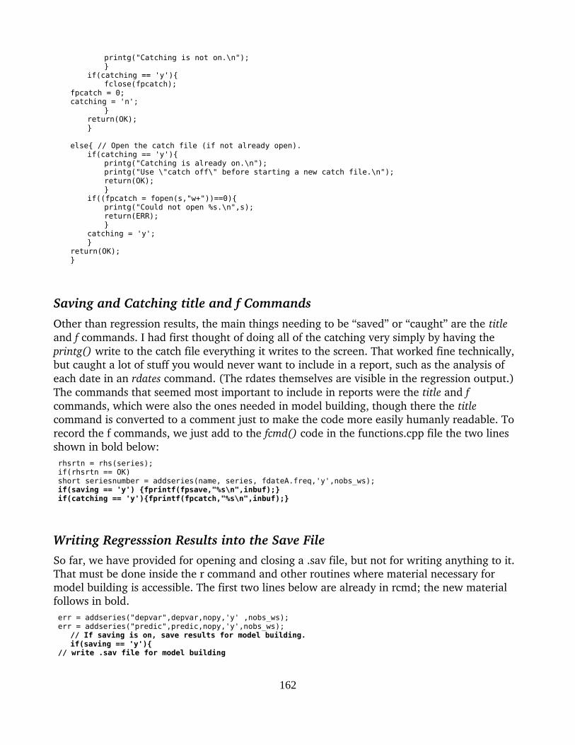
printg("Catching is not on.\n");}
if(catching == 'y'){fclose(fpcatch);
fpcatch = 0; catching = 'n';
}return(OK);}
else{ // Open the catch file (if not already open).if(catching == 'y'){
printg("Catching is already on.\n");printg("Use \"catch off\" before starting a new catch file.\n");return(OK);}
if((fpcatch = fopen(s,"w+"))==0){printg("Could not open %s.\n",s);return(ERR);}
catching = 'y';}
return(OK);}
Saving and Catching title and f CommandsOther than regression results, the main things needing to be “saved” or “caught” are the title and f commands. I had first thought of doing all of the catching very simply by having the printg() write to the catch file everything it writes to the screen. That worked fine technically, but caught a lot of stuff you would never want to include in a report, such as the analysis of each date in an rdates command. (The rdates themselves are visible in the regression output.) The commands that seemed most important to include in reports were the title and f commands, which were also the ones needed in model building, though there the title command is converted to a comment just to make the code more easily humanly readable. To record the f commands, we just add to the fcmd() code in the functions.cpp file the two lines shown in bold below: rhsrtn = rhs(series); if(rhsrtn == OK) short seriesnumber = addseries(name, series, fdateA.freq,'y',nobs_ws); if(saving == 'y') {fprintf(fpsave,"%s\n",inbuf);} if(catching == 'y'){fprintf(fpcatch,"%s\n",inbuf);}
Writing Regresssion Results into the Save FileSo far, we have provided for opening and closing a .sav file, but not for writing anything to it. That must be done inside the r command and other routines where material necessary for model building is accessible. The first two lines below are already in rcmd; the new material follows in bold. err = addseries("depvar",depvar,nopy,'y' ,nobs_ws); err = addseries("predic",predic,nopy,'y',nobs_ws);
// If saving is on, save results for model building. if(saving == 'y'){ // write .sav file for model building
162

fprintf(fpsave,"r %s = %12.6f",ptitles[0],a[1][0] ); if(niv >1){ for(i = 2;i< niv;i++){ fprintf(fpsave," +\n %12.6f * %s",a[i][0],ptitles[i]); } } fprintf(fpsave,"\n"); fprintf(fpsave,"d\n\n"); }
This looks quite simple at first glance, but it is a little tricky. We always write the first regression coefficient; then if there are more, we write a + and then a newline and then the next coefficient. After the last coefficient, however, no + is written, only the newline. On the line below the last coefficient, a d is written, followed by two newlines. No one seems to remember what the d stands for, maybe “done” or maybe “demarcation.” But the Build program expects it, so we keep the tradition.
Writing Regression Results into the Catch FileWriting the regression results into the Catch file is just a matter of repeating the printg()
commands which wrote results to the screen as fprintf() commands if catching is on.The new code in rcmd.cpp is shown in bold. // Print the results. // Center the title j = (MAXCHARINTITLE - strlen(title))/2;
for(i=1;i<j;i++) buf[i] = ' '; buf[0] =':'; buf[j] = '\0'; printg("%s",buf); printg(" %s \n",title); printg("SEE = %10.1f RSQ = %8.3f RHO = %8.3f DW = %8.3f\n",see,rsq,rho,dw); printg(" Variable name RegCoef Mexval Elas NorRes Means\n"); if (catching == 'y'){ fprintf(fpcatch,"%s",buf); fprintf(fpcatch," %s \n",title); fprintf(fpcatch,"SEE = %10.1f RSQ = %8.3f RHO = %8.3f DW = %8.3f\n",see,rsq,rho,dw); fprintf(fpcatch," Variable name RegCoef Mexval Elas NorRes Means\n"); }
for (i = 1;i <= niv;i++){ mexval =100.*(safesqrt(1.+ (a[i][0]*a[i][0]/
(a[i][i]*a[0][0])))-1.);
student = a[i][0]/safesqrt(a[i][i]*sigma_sq);elas = norresid = 0;if(means[0]!=0) elas = a[i][0]*means[i]/means[0];if(rpr[niv] > 0) norresid = rpr[i]/rpr[niv];if(norresid > 9999.99) norresid = 9999.99;printg(" %2d %-20s ",i,ptitles[i]);printg(" %10.5f %7.1f",a[i][0],mexval);printg(" %6.2f %7.2f %9.2f\n",elas,norresid,means[i]);
//if(i == 0 && showt) printg(" %7.3f",student); if(catching == 'y'){ fprintf(fpcatch, " %2d %-20s ",i,ptitles[i]); fprintf(fpcatch," %10.5f %7.1f",a[i][0],mexval); fprintf(fpcatch," %6.2f %7.2f %9.2f\n",elas,norresid,means[i]); } }
163
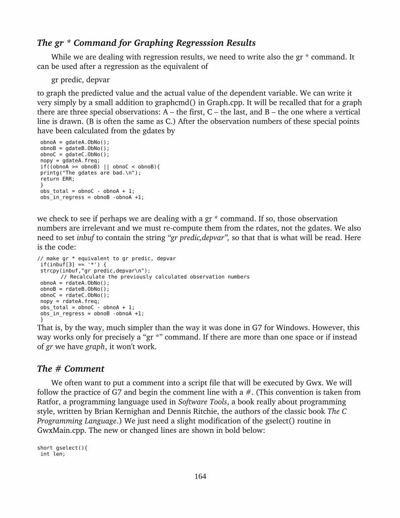
The gr * Command for Graphing Regresssion ResultsWhile we are dealing with regression results, we need to write also the gr * command. It
can be used after a regression as the equivalent of
gr predic, depvar
to graph the predicted value and the actual value of the dependent variable. We can write it very simply by a small addition to graphcmd() in Graph.cpp. It will be recalled that for a graphthere are three special observations: A – the first, C – the last, and B – the one where a vertical line is drawn. (B is often the same as C.) After the observation numbers of these special points have been calculated from the gdates by obnoA = gdateA.ObNo(); obnoB = gdateB.ObNo(); obnoC = gdateC.ObNo(); nopy = gdateA.freq; if((obnoA >= obnoB) || obnoC < obnoB){ printg("The gdates are bad.\n"); return ERR; } obs_total = obnoC - obnoA + 1; obs_in_regress = obnoB -obnoA +1;
we check to see if perhaps we are dealing with a gr * command. If so, those observation numbers are irrelevant and we must recompute them from the rdates, not the gdates. We alsoneed to set inbuf to contain the string “gr predic,depvar”, so that that is what will be read. Here is the code:// make gr * equivalent to gr predic, depvar if(inbuf[3] == '*') { strcpy(inbuf,"gr predic,depvar\n");
// Recalculate the previously calculated observation numbers obnoA = rdateA.ObNo(); obnoB = rdateB.ObNo(); obnoC = rdateC.ObNo(); nopy = rdateA.freq; obs_total = obnoC - obnoA + 1; obs_in_regress = obnoB -obnoA +1; }
That is, by the way, much simpler than the way it was done in G7 for Windows. However, this way works only for precisely a “gr *” command. If there are more than one space or if instead of gr we have graph, it won't work.
The # CommentWe often want to put a comment into a script file that will be executed by Gwx. We will
follow the practice of G7 and begin the comment line with a #. (This convention is taken from Ratfor, a programming language used in Software Tools, a book really about programming style, written by Brian Kernighan and Dennis Ritchie, the authors of the classic book The C Programming Language.) We just need a slight modification of the gselect() routine in GwxMain.cpp. The new or changed lines are shown in bold below:
short gselect(){ int len;
164

short err; char s[100],choprtn; while ((choprtn = chop(s)) != 'e'){ len = strlen(s); if(strncmp(s,"type",std::max(len,2)) == 0) err = typecmd(); else if(choprtn == '#') continue; else if(strncmp(s,"fex",std::max(len,1)) == 0) err = fcmd();
The comment will show up on the screen as the file is executed but will not be included in the catch file if one is being created, something we may want to change.
165

Tutorial 15: Softly Constrained Regression: The con and smaCommands
Soft ConstraintsEconometric textbooks generally proceed under the assumption that there is a true
equation of the form we are fitting though we may be unsure about whether or not some variable belongs in the equation. They assume further that, though we know the form precisely, we know nothing of the values of the parameters. Of course, nothing could be farther from the truth. Generally we are fitting a very simple equation to a vastly complicated reality. There is no true equation of the form we are fitting. We are just trying to get a workable description of that complex reality. Probably all of the variables belong in the equation, and we have some ideas about the values of the parameters being estimated. Economists are in a very different position in this respect from a natural scientist. No physiscistwould ask himself “What would you do if you were an electron?” No microbiologist asks “Whatwould you do if you were a bacterium?” But the economist may well ask, “What would you do if you were a consumer?” Indeed, it is the answers to this sort of question which constitute economic theory.
In using regression analysis for model building, this a priori knowledge may take the form of reasonable values of regression coefficients or reasonable values for sums or other linear combinations of regression coefficients. Our job in this tutorial is to convey such information tothe regression program. We will do so, not as hard and fast constraints which must be satisfied, but in a way that has the program find a compromise between closeness of fit to the data and conformity to our a priori expectations. We say that constraints applied in this way are soft constraints.
We will apply a linear constraint softly by adding artificial observations to the natural observations of the data. For example, if we want
5 = 1b1+2b2+1 b3
we just add the observation
5 1 2 1
where 5 is the dependent variable and 1, 2 and 1 are the values of the first three independent variables. Note that if the b's satisfy the above equation, this “observation” will have a zero error. So as we add more and more such observations, we will gently, softly “pull” the b's to satisfy the equation. The con command allows the user to impose softly any desired linear constraint on the regression coefficients. The constraint is made “harder” and harder the more artificial observations are added, so we will include in the command to add an observation the number of times that observations is added.
Often the constraint that we want to impose is that a number of coefficients lie on a loworder polynomial such as a straight line or a quadratic or cubic curve. Often these coefficients are weights in a distributed lag. The sma command, developed in the second part of this tutorial,
166

makes it easy to softly impose a polynomial pattern on distributed lag weights. The sma name comes from the initials of Shirley Montag Almon, who was the first to use polynomials for distributed lag weights.
The con CommandThe general form of the constraint or con command is
con <count> <left> = <right>where
count is the number of artificial observations per natural observation.left is a number, the left side of the equation which expresses the constraint.right is any linear expression in the coefficients of the equation.
Some examples of con commands illustrating the right” element are‟
con 3 .9 = a2con 200 0 = a2 - 2a3 + a4con 1000 1 = a3 + a4 + a5 + a6 .
The letter a is used here to denote the regression coefficients instead of the b which we have usually used because we may wish to extend Gwx to be able (as G7 is) to estimate severalregression equations at once with constraints across the equations. In such tasks, a is used for the coefficients of the first equation, b for coefficients of the second, and so on. For the time being, however, it does not matter what letter is used.
The natural question at this point is: “How do I know how many of the artificial observations to use?” Is it really conceivable that, as the third example seems to imply, I wouldever want to use 1000 artificial observations per natural observation? The only general rule about how many to use is As many as it takes to accomplish what you want done.” And yes, it‟is quite common to take large numbers of artificial observations, because their impact dependson the dimensions of the variables. Suppose, as in the third example above, that we are trying to constraint the sum of four coefficients, all of them between 0 and 1, to be 1.0. The discrepancy is likely to be .2 or .4 at worst. Now if the dimension of the dependent variable is such that the SEE for the equation is 1200, then it is going to take a lot of observations with anerror of .2 to make the leastsquares algorithm listen” to the constraint. Indeed, it is going to ‟take a thousand, or maybe ten thousand. Experiment to find out what it takes for your particular equation.
Now to get down to business and writing the code for con. To keep the code simple, we will follow the example of G7 and specify a maximum number of constraints, MAXCON, and a matrix, conprm, to hold the “count” and “left” values for each constraint, and a matrix, constraints, to hold the right-hand side of the constraints. We will also use a GLOBAL short integer, concount, to count the number of constraints in use. These are specified in the common.h file by adding the lines shown in bold below.
#define MAXVAR 30 // Maximum number of variables in a regression
#define MAXCON 30 // Maximum number of constraints in a regression#define MAXCHARINTITLE 80. . . .
167

GLOBAL char keyboard; // 'y' when input is from keyboard; 'n' when input is from a file.GLOBAL float **xp; //xp is where the matrix of observations for regression is storedGLOBAL float **zp; //zp is where the data for graphs is stored
GLOBAL float constraints[MAXCON][MAXVAR],conprm[MAXCON][2];GLOBAL float GraphRange[2],vrange[11];GLOBAL short vrflag;GLOBAL short legendcount;GLOBAL char Legend[4][MAXCHARINLEGEND];GLOBAL char BankType[MAXBANK]; // 'w','c','g','v'GLOBAL short NumAssigned; // Number of assigned banks.GLOBAL char DefaultVam;GLOBAL char saving, catching;
GLOBAL short concount;GLOBAL FILE *fpsave,*fpcatch;
Our first business is to be sure that concount is initialized to zero when the program starts. We won't bother to initialize the two matrices, constraints and conprm, in advance, but will clear each row to zero just before putting data into it. Initializing of concount is done, of course, in OnCreate() in GwxMain.cpp, like this:
void GwxFrame::OnCreate(wxWindowCreateEvent& event){ short i; printout[0] = '\0';
. . . . . MaxRegVar = MAXVAR; MaxRegObs = NOMAX; vrflag = 0; saving = 'n'; catching = 'n';
concount = 0;. . . .
}
Then, to make Gwx detect and act on the con command, we need to add in the gselect() routine found in the GwxMain.cpp module, the first line shown in bold below. Since we will soon be coming back in this tutorial to add the sma command, we may as well add the call to it now, so its call appears in the second line set in bold below.
else if (strncmp(s,"save",std::max(len,3)) == 0) err = savecmd(); else if (strncmp(s,"catch",std::max(len,3)) == 0) err = catchcmd();
else if (strncmp(s,"constraint",std::max(len,3)) == 0) err = concmd();else if (strncmp(s,"sma",3)== 0) err = smacmd();else if (strncmp(s,"tdates",std::max(len,2)) == 0) err = tdatescmd();
Just to test these two lines we can put at the end of the rcmd.cpp module these dummy routines. int smacmd(){ printg("Hello from SMA!\n"); return OK; }int concmd(){ printg("Hello from ConCmd!\n"); return OK; }
(When I first tried this, I got the parentheses wrong in the call to ConCmd, and it took a long time to make it work.)
168

The whole of the concmd() is shown in the box below. Here we comment on some of the lines that call for explanation.
// Clear the comcount row of the constraints and conprm matrices. for(i = 0;i< MAXCON;i++) constraints[concount][i] = 0.; for(i =0; i <=1;i++) conprm[concount][i] = 0;
Remember that we did not clear these matrices initially because we clear them here.// Get count choprtn = chop(datum); if(choprtn == 'n') count = atof(datum); else { printg("Bad count in con command. Need a number.\n"); geteol(); return ERR; }
The count, the number of artificial observations per natural observation must be a positive number, but not necessarily an integer.// Get left side of constraint choprtn = chopnumber(datum); if(choprtn == 'n') left = atof(datum); else { printg("Bad left side in con command. Need a nimber.\n"); geteol(); return ERR; }
The left side of the constraint must be a number, but not necessarily positive, so we use the chopnumber() function we introduced back on page 58.
Now comes a bit of rather subtle code. Remember that we may be reading a line which looks like this:
5 7 = a5 – 2a5 +1.3a7 – a8
We have got to interpret the lack of a number in front of the a as a 1. The variable coef is going to become the number in front of the a or other letter and neg is going to end up as +1 or 1 according to whether the term has a + or sign. Since it has been a while since we used chop(), I remind you that when it hits a number it returns n and the the ASCII string representing the number (including a possible decimal point) is in the argument, here called datum. When chop() hits a letter, it returns a and the string it found, including numbers, is in the argument. When it hits an end of line, it returns e. We start off assuming that the coefficient is +1. printg("Hello from ConCmd!\n"); // Now go for the right side. choprtn = chop(datum); // skip the = sign neg = 1.; coef =1;
In a properly written con command, when we again call chop(), we hit either a
in which case we make neg = 1
or an
169

+ in which case we make neg = +1
or a number, which we convert into the absolute value of coefficient
or a letter followed by a number. We ignore the letter, and convert the number to an integer to tell us into which column of the constraints matrix the (properly signed) coef goes.
Here is the code.
while((choprtn = chop(datum)) != 'e'){ if(choprtn == '-'){ neg = -1.; } else if (choprtn == '+') { neg = 1.; } else if (choprtn == 'n'){ coef = atof(datum); } else if (choprtn == 'a') { col = atoi(&datum[1]);// this skips the letter and gets the number coef = neg*coef; constraints[concount][col] = coef; // printg("column %d coef %10.3f\n",col,coef); neg = 1.; coef = 1.; } }
The rest of the code is routine. Here is the whole of the concmd.int concmd(){ char datum[32]; char choprtn; float count,left,neg,coef; short col,i; if(concount >= MAXCON){ printg("Maximum number of constraints,%d, exceeded.\n",concount); } // Clear the comcount row of the constraints and conprm matrices. for(i = 0;i< MAXCON;i++) constraints[concount][i] = 0.; for(i =0; i <=1;i++) conprm[concount][i] = 0;
// Get count choprtn = chopnumber(datum); if(choprtn == 'n') count = atof(datum); else { printg("Bad count in con command. Need a number.\n"); geteol(); return ERR; }// Get left side of constraint choprtn = chopnumber(datum); if(choprtn == 'n') left = atof(datum); else { printg("Bad left side in con command. Need a nimber.\n"); geteol(); return ERR; } printg("Hello from ConCmd!\n"); printg("Count = %10.1f Left = %10.1f\n",count,left); // Now go for the right side. choprtn = chop(datum); // skip the = sign
170
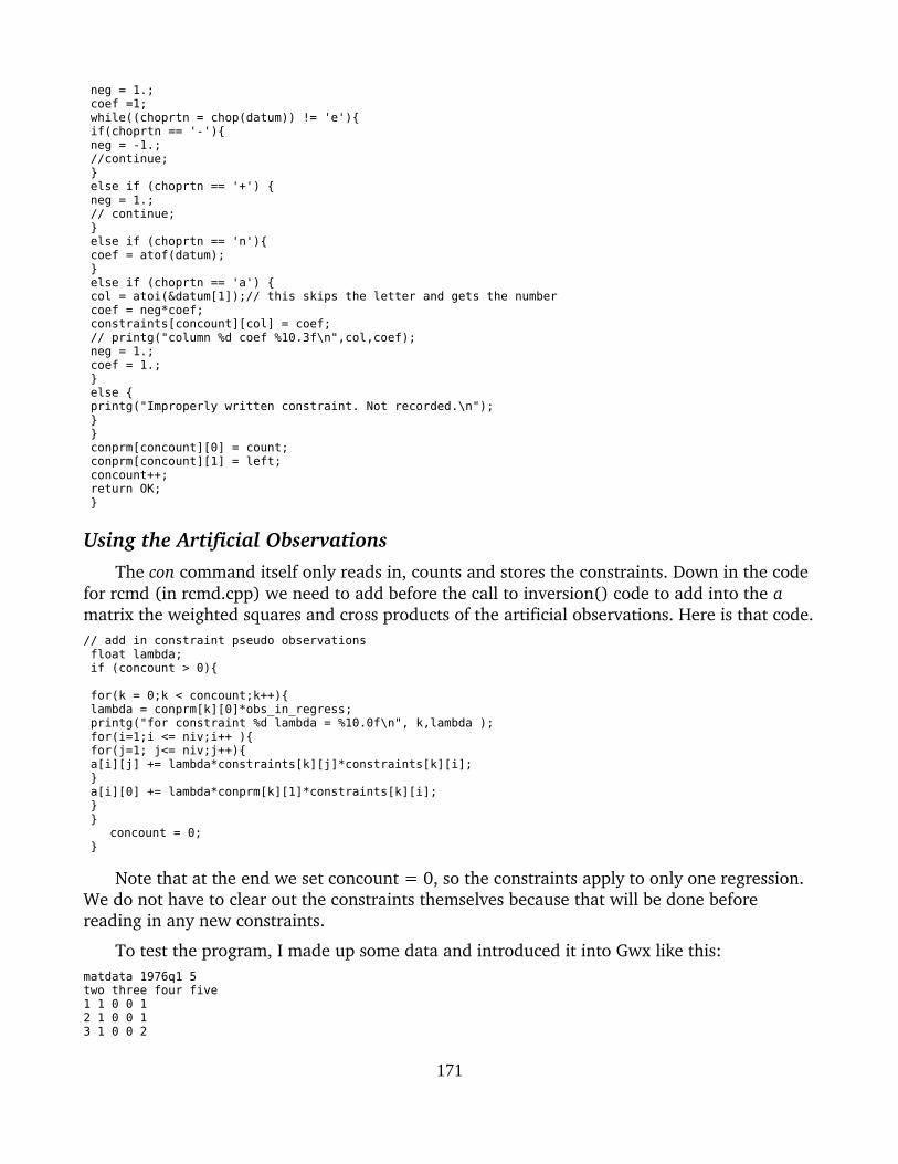
neg = 1.; coef =1; while((choprtn = chop(datum)) != 'e'){ if(choprtn == '-'){ neg = -1.; //continue; } else if (choprtn == '+') { neg = 1.; // continue; } else if (choprtn == 'n'){ coef = atof(datum); } else if (choprtn == 'a') { col = atoi(&datum[1]);// this skips the letter and gets the number coef = neg*coef; constraints[concount][col] = coef; // printg("column %d coef %10.3f\n",col,coef); neg = 1.; coef = 1.; } else { printg("Improperly written constraint. Not recorded.\n"); } } conprm[concount][0] = count; conprm[concount][1] = left; concount++; return OK; }
Using the Artificial ObservationsThe con command itself only reads in, counts and stores the constraints. Down in the code
for rcmd (in rcmd.cpp) we need to add before the call to inversion() code to add into the a matrix the weighted squares and cross products of the artificial observations. Here is that code.// add in constraint pseudo observations float lambda; if (concount > 0){
for(k = 0;k < concount;k++){ lambda = conprm[k][0]*obs_in_regress; printg("for constraint %d lambda = %10.0f\n", k,lambda ); for(i=1;i <= niv;i++ ){ for(j=1; j<= niv;j++){ a[i][j] += lambda*constraints[k][j]*constraints[k][i]; } a[i][0] += lambda*conprm[k][1]*constraints[k][i]; } }
concount = 0; }
Note that at the end we set concount = 0, so the constraints apply to only one regression. We do not have to clear out the constraints themselves because that will be done before reading in any new constraints.
To test the program, I made up some data and introduced it into Gwx like this:matdata 1976q1 5 two three four five 1 1 0 0 1 2 1 0 0 1 3 1 0 0 2
171

4 0 1 0 2 5 0 1 0 2 6 0 1 0 3 7 0 0 1 3 8 0 0 1 3 9 0 0 1 4 ;
Then I regressed variable “five” on the other three like so:
rdates 1976q1 1978q1 1978q1 tdates 1976q1 1978q1 ti no constaint r five = two,three,four
with these results:: no constaint SEE = 0.5 RSQ = 0.797 RHO = -0.042 DW = 2.085 Variable name RegCoef Mexval Elas NorRes Means 1 intercept 0.00000 0.0 0.00 7.47 1.00 2 two 1.42857 46.8 0.20 6.49 0.33 3 three 2.42857 108.2 0.35 6.38 0.33 4 four 3.14286 152.5 0.45 1.00 0.33
Then I added in the soft constraint that I wanted the coefficient on “two” to be about 3 and repeated the regression,ti constaint on a2 con 10 3 = 1a2 r five = two,three,four
with these results:: constaint on a2 SEE = 0.6 RSQ = 0.730 RHO = 0.346 DW = 1.307 Variable name RegCoef Mexval Elas NorRes Means 1 intercept -1.25794 -100.0 -0.54 0.00 1.00 2 two 2.98602 -100.0 0.43 0.00 0.33 3 three 3.56671 -100.0 0.51 0.00 0.33 4 four 4.22109 -100.0 0.60 0.00 0.33
The coefficient on “two” came up very close to the softconstraint value of 3.0 with an increase in the SSR and reduction in RSQ, and some changes in the other regression coefficients. Since that is the expected result, I presume we have gotten the coding right.
In the process of testing this example, however, I learned of a slightly disturbing problem. At first, I had the madeup data and the regression begin in 1975q1, the period in which the workspace begins, as determined by Gwx.cfg. Then when the program got to the point where it deletes the predic vector at the end of rcmd(), it crashed. Why it should do so, I do not understand. Moving the data forward so that the first observation in the workspace is not usedavoided the problem. I have not been able to see any problem in the code that would produce the behavior. For the moment, it is easy enough to avoid the problem.
The sma command for estimating distributed lagsCauses do not always have their effects immediately. When companies appropriate funds
for capital investment, the expenditures that follow are spread over eight or more quarters, that is, with a distributed lag after the appropriation. An increase in output stimulates investment which follows with a distributed lag. An increase in personal income leads to
172

increased consumption with a distributed lag. A change in the exchange rate leads to changes in exports and imports with a distributed lag. Clearly, estimating these lags is an important component of econometric technique. Sometimes it is done by including a lagged value of the dependent variable in the equation. If all one wants is to forecast one period ahead, such an equation is hard to beat. But if one wants to understand causes and effects, this is a dangerous device. The lagged value sums up perfectly all the influences on the dependent variable as of one period earlier. If the period is short, that summary is still very good for the current period, and the lagged value does most of the explanation, robbing the other variables of their proper importance. The fit of the equation will be splendid, but it will perform poorly in forecasts going many periods ahead and will give misleading results in policy simulations. It is generallymuch better to introduce the lagged values of the independent variables explicitly and to estimate the distributed lag directly. These lagged values, however, will often be very collinearand the regression coefficients on the successive lagged values will jump about in a highly implausible fashion. This problem has led to the development of various ways to impose “plausibility” on the regression coefficients. An early proposal was to make the weights lie on inverted V. Much more successful was the method introduced and applied by Shirley M. Almonthat made the weights follow precisely a polynomial of low degree, typically third or fourth. This method found wide application, but had the problem that weights near the end of the lag often came out negative. Robert J. Shiller then suggested softly constraining the weights to lie on a polynomial. This method largely eliminated the problem with small negative weights at the end of the lag, and is the method we will implement here. I have retained the name sma for the command because it was Shirley Almon's pioneering work that popularized polynomial lags.
How can one softly impose the requirement that weights lie on a polynomial? If the equally spaced weights lie in a straight line, their first differences will be constant, and their second differences – the differences of the first differences – will be zero. Conversely, if the second differences are zero, the first differences must be constant, and the weights must lie in a straight line. Thus, overlapping linear constraints softly requiring that all the second differences be zero softly requires that all the weights lie on a straight line.
What about higher degree polynomials? The first differences of equally spaced points on a polynomial of degree n lie on a polynomial of degree n1 as is easily seen:
an t n+P (n−1)−(an( t − 1)
n+ P(n−1)) = P (n−1)
where P(n1) represents any polynomial of degree n1 in t. So the third differences of weights lying on a parabola are zero; the fourth differences of the weights lying on a cubic polynomial are zero, and so on. So we just need to be able to express these differences in terms of the original weights – which will be regression coefficients. Here is a table showing successive differences in terms of the original weights.
173

We immediately recognize the familiar pattern of Pascal's triangle and binomial coefficients. We just need a way for the user to generate easily the required linear constraints and add them to any that may have been created by the con command. That is what the sma command does. The format of the command is:
sma <top> <aStart> <aStop> <n> [f]
where: top is the tradeoff parameter specifying our tradeoff between closeness of fit to the data and and closeness of adherence to the polynomial form of the weights. Start is the number of the regression coefficient where the lag begins.Stop is the number of the regression coefficient where the lag stops.n is the order of the polynomial.f is an optional parameter to indicate that the end of the lag should be free or floating.
Without the f, the program assumes that the weight next after the last one estimated is zero, and thus ties down the end of the distribution.
The Start and Stop numbers are preceded by a letter to keep the command consistent withthe G7 command which allows constraints across equations, a seldom if ever used feature I do not intend to implement in Gwx. The code is largely borrowed from G7 where it has been littleif at all changed from what I originally wrote.
int smacmd(){
int i,j,order,first,last,new_con,first_con,a,ieq;char s[80],tflag;float top;
/* Get trade-off parameter */if ((chop(s)) == 'n')
top = atof(s);else{
printg("Expected a number for the trade-off parameter.\n");return(ERR);}
/* Get first coefficient constrained */if ((chop(s)) == 'a'){
a = s[0];ieq = a - 97; /* 97 is ascii constant for 'a' */first = atoi(&s[1]);}
else{
174
Weight First difference Second difference Third difference Fourth differencew1
w1 – w2w2 1w1 -2w2 + 1w3
w2 – w3 1w1 – 3w2 + 3w3 – 1w4w3 1w2 -2w3 + 1w4 1w1 – 4w2 + 6w3 – 4w4 + w5
w3 – w4 1w2 – 3w3 + 3w4 – 1w5w4 1w3 -2w4 + 1w5
w4 - w5w5
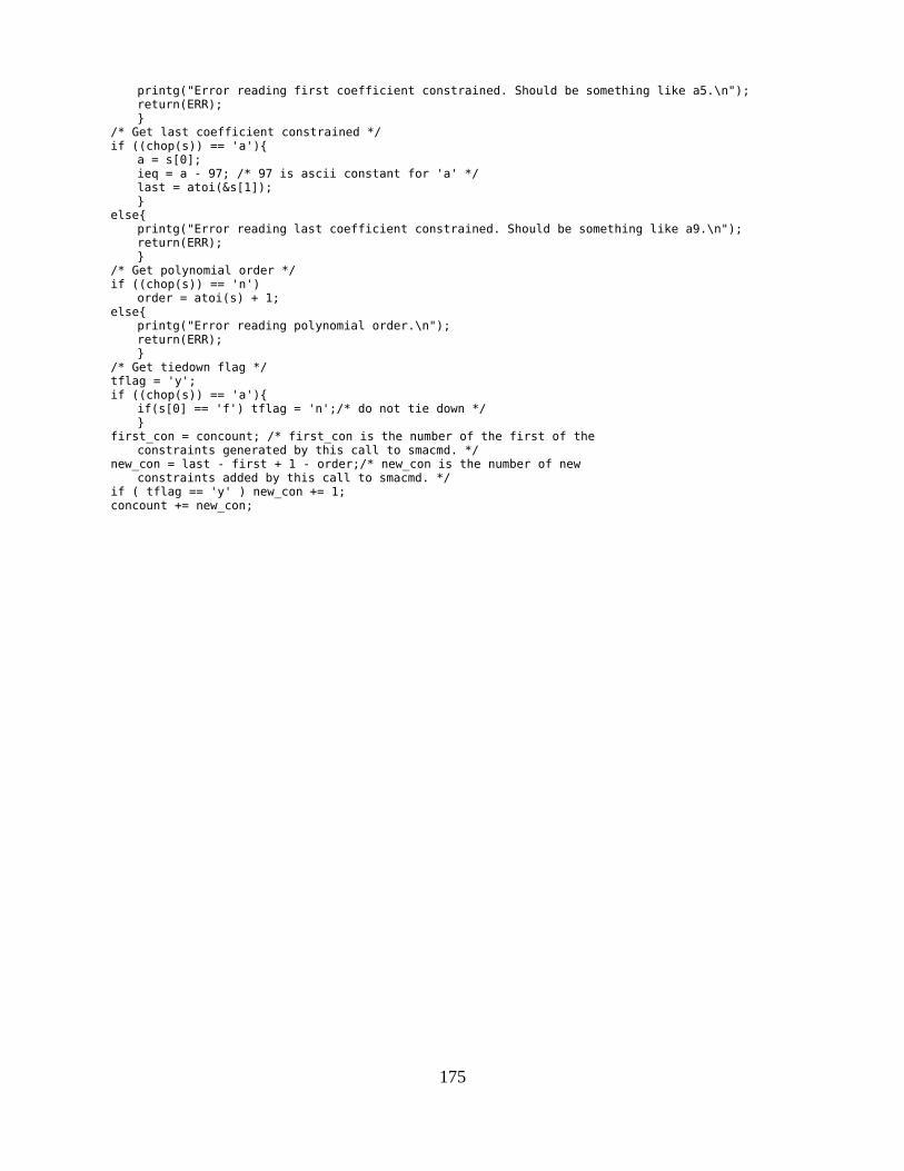
printg("Error reading first coefficient constrained. Should be something like a5.\n");return(ERR);}
/* Get last coefficient constrained */if ((chop(s)) == 'a'){
a = s[0];ieq = a - 97; /* 97 is ascii constant for 'a' */last = atoi(&s[1]);}
else{printg("Error reading last coefficient constrained. Should be something like a9.\n");return(ERR);}
/* Get polynomial order */if ((chop(s)) == 'n')
order = atoi(s) + 1;else{
printg("Error reading polynomial order.\n");return(ERR);}
/* Get tiedown flag */tflag = 'y';if ((chop(s)) == 'a'){
if(s[0] == 'f') tflag = 'n';/* do not tie down */}
first_con = concount; /* first_con is the number of the first of theconstraints generated by this call to smacmd. */
new_con = last - first + 1 - order;/* new_con is the number of newconstraints added by this call to smacmd. */
if ( tflag == 'y' ) new_con += 1;concount += new_con;
175
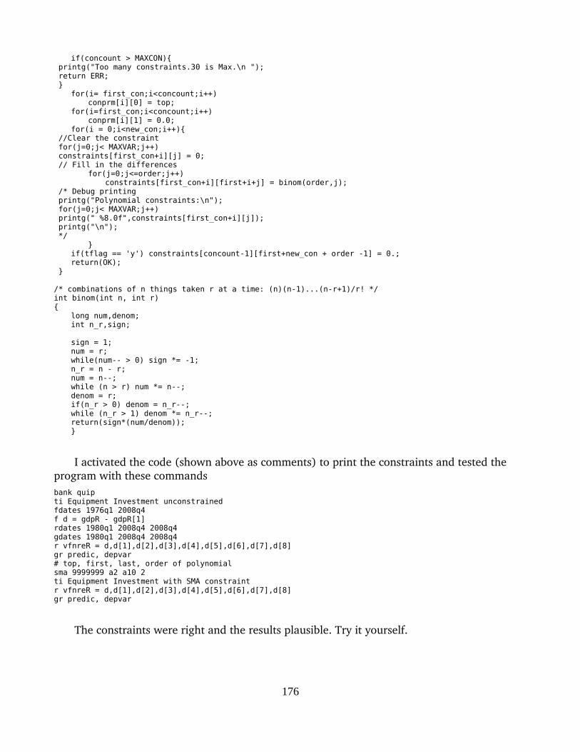
if(concount > MAXCON){ printg("Too many constraints.30 is Max.\n "); return ERR; }
for(i= first_con;i<concount;i++)conprm[i][0] = top;
for(i=first_con;i<concount;i++)conprm[i][1] = 0.0;
for(i = 0;i<new_con;i++){ //Clear the constraint for(j=0;j< MAXVAR;j++) constraints[first_con+i][j] = 0; // Fill in the differences
for(j=0;j<=order;j++)constraints[first_con+i][first+i+j] = binom(order,j);
/* Debug printing printg("Polynomial constraints:\n"); for(j=0;j< MAXVAR;j++) printg(" %8.0f",constraints[first_con+i][j]); printg("\n"); */
}if(tflag == 'y') constraints[concount-1][first+new_con + order -1] = 0.;return(OK);
}
/* combinations of n things taken r at a time: (n)(n-1)...(n-r+1)/r! */int binom(int n, int r){
long num,denom;int n_r,sign;
sign = 1;num = r;while(num-- > 0) sign *= -1;n_r = n - r;num = n--;while (n > r) num *= n--;denom = r;if(n_r > 0) denom = n_r--;while (n_r > 1) denom *= n_r--;return(sign*(num/denom));}
I activated the code (shown above as comments) to print the constraints and tested the program with these commandsbank quip ti Equipment Investment unconstrained fdates 1976q1 2008q4 f d = gdpR - gdpR[1] rdates 1980q1 2008q4 2008q4 gdates 1980q1 2008q4 2008q4 r vfnreR = d,d[1],d[2],d[3],d[4],d[5],d[6],d[7],d[8] gr predic, depvar # top, first, last, order of polynomial sma 9999999 a2 a10 2 ti Equipment Investment with SMA constraint r vfnreR = d,d[1],d[2],d[3],d[4],d[5],d[6],d[7],d[8] gr predic, depvar
The constraints were right and the results plausible. Try it yourself.
176

Tutorial 16. Useful FunctionsAt this point, Gwx is approaching actually being useful for estimating the equations of a
macro model. It needs, however, several more frequently used functions such as:
@cum() to create stocks from flows
@atoq() to make a quarterly series from an annual one
@atoqi() to make a quarterly series from an annual one with an indicator
@mtoq() to make a quarterly series from an monthly one
Back in Tutorial 10 on page 101 we have already introduced @log() and @exp(), and we will follow their pattern in writing the above functions. We need to recall that in the rhs() function (in the functions.cpp module) we have the code case '@':
if((functions(y) != OK)) {go = STOP;rhsrtn = ERR;goto closeup;}
if(muldiv(x,y,obnoA,obnoB,op_stack, &osp) == ERR){ rhsrtn = ERR; goto closeup; } break;
where y is a vector which will be filled by the values of the function. So to remind ourselves of how to write an “@ function” we need to have a look at the functions() routine in the functions.cpp module. There we find the following code to which the line in bold has been added for the @cum() function:short functions(float *f){
char err,s[MAXNAMELENGTH];short funcrtn;
funcrtn = OK;
if ((err = chop(s)) != 'a'){printg("Following a @ must come a function name.\n");return ERR;}
if (strcmp(s,"log") == 0) funcrtn = logarithm(f); else if (strcmp(s,"exp") == 0) funcrtn = exponential(f);
else if (strcmp(s,"cum") == 0) funcrtn = cumulate(f); else { printg("Unrecognized function %s.\n",s); funcrtn = ERR; } return funcrtn; }
All of our additions to Gwx's library of functions will begin by adding here an else if line similar to the one shown here for the @cum() function.
Create Stocks from Flows – @cum() This function creates a stock variable from a flow variable from this formula:
177
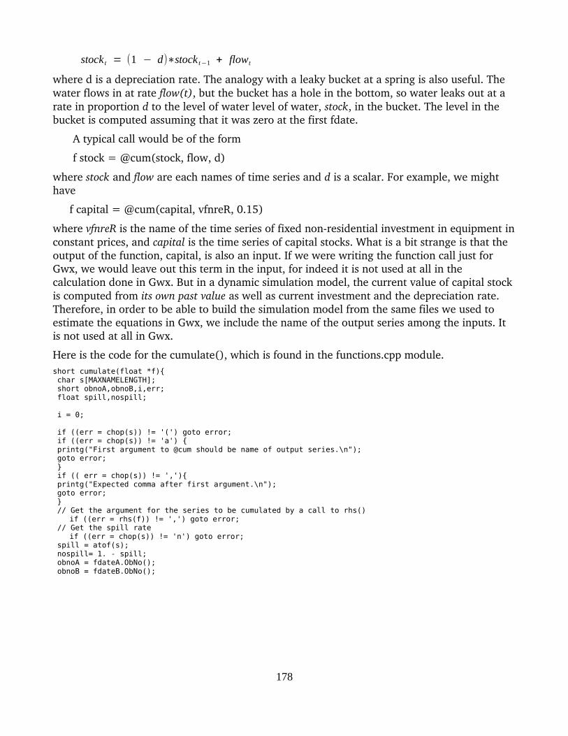
stock t = (1 − d)∗stock t−1 + flowt
where d is a depreciation rate. The analogy with a leaky bucket at a spring is also useful. The water flows in at rate flow(t), but the bucket has a hole in the bottom, so water leaks out at a rate in proportion d to the level of water level of water, stock, in the bucket. The level in the bucket is computed assuming that it was zero at the first fdate.
A typical call would be of the form
f stock = @cum(stock, flow, d)
where stock and flow are each names of time series and d is a scalar. For example, we might have
f capital = @cum(capital, vfnreR, 0.15)
where vfnreR is the name of the time series of fixed nonresidential investment in equipment inconstant prices, and capital is the time series of capital stocks. What is a bit strange is that the output of the function, capital, is also an input. If we were writing the function call just for Gwx, we would leave out this term in the input, for indeed it is not used at all in the calculation done in Gwx. But in a dynamic simulation model, the current value of capital stock is computed from its own past value as well as current investment and the depreciation rate. Therefore, in order to be able to build the simulation model from the same files we used to estimate the equations in Gwx, we include the name of the output series among the inputs. It is not used at all in Gwx.
Here is the code for the cumulate(), which is found in the functions.cpp module.short cumulate(float *f){ char s[MAXNAMELENGTH]; short obnoA,obnoB,i,err; float spill,nospill;
i = 0;
if ((err = chop(s)) != '(') goto error; if ((err = chop(s)) != 'a') { printg("First argument to @cum should be name of output series.\n"); goto error; } if (( err = chop(s)) != ','){ printg("Expected comma after first argument.\n"); goto error; } // Get the argument for the series to be cumulated by a call to rhs()
if ((err = rhs(f)) != ',') goto error; // Get the spill rate
if ((err = chop(s)) != 'n') goto error; spill = atof(s); nospill= 1. - spill; obnoA = fdateA.ObNo(); obnoB = fdateB.ObNo();
178

// Do the cumulation:
for( i = obnoA+1; i <= obnoB; i++){ f[i] = f[i] + nospill*f[i-1]; } return OK;
error: return ERR; }
I thought that was all that was necessary. But I was wrong. When reading the arguments of a command like @cum(capital, vfnreR, 0.15) the comma after the end of the second argument must stop the reading of the expression. This is the first time we have had to stop reading an expression when we hit a comma, and we were not ready. So in the rhs() function in functions.cpp, where we formerly had just case ')': rhsrtn = OK; go = STOP; break;
we now have case ')': rhsrtn = ')'; go = STOP; break;
case ',': rhsrtn = ','; go = STOP; break;
where I preserved the distinction between the ')' and the ',' termination which may possibly be useful in the future. At present, however, it only made trouble elsewhere, namely in fcmd() (inthe functions.cpp module) where we previously had just
rhsrtn = rhs(series);if(rhsrtn == OK ) seriesnumber = addseries(name, series, fdateA.freq,'y',nobs_ws);
we now need for the second line
if(rhsrtn == OK || rhsrtn == ')') seriesnumber = addseries(name,series,fdateA.freq,'y',nobs_ws);
That is not so bad if you remember that you need to make the change. But I did not remember and spent an hour or more trying to understand why the new, cumulated series was not appearing in the data bank. We do not need to add the series which precedes the comma in the @cum() command to the data bank, so all now seems well.
Frequency conversion by polynomial interpolationMaking making a series of one frequency from one of a lower frequency obviously involves data creation, and there is no perfect way to do it. All we can hope for is plausibility. We will assume that the series are flows – such as GDP or investment – not values of a specific date, such as stock exchange closing prices. We therefore want the sum of the four quarterly values
179
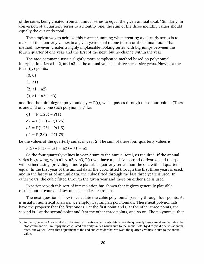
of the series being created from an annual series to equal the given annual total.5 Similarly, in conversion of a quarterly series to a monthly one, the sum of the three monthly values should equally the quarterly total.
The simplest way to achieve this correct summing when creating a quarterly series is to make all the quarterly values in a given year equal to one fourth of the annual total. That method, however, creates a highly implausiblelooking series with big jumps between the fourth quarter of one year and the first of the next, but no change within the year.
The atoq command uses a slightly more complicated method based on polynomial interpolation. Let a1, a2, and a3 be the annual values in three successive years. Now plot the four (t,y) points:
(0, 0)
(1, a1)
(2, a1+ a2)
(3, a1+ a2 + a3),
and find the third degree polynomial, y = P(t), which passes through these four points. (Thereis one and only one such polynomial.) Let
q1 = P(1.25) – P(1)
q2 = P(1.5) – P(1.25)
q3 = P(1.75) – P(1.5)
q4 = P(2.0) – P(1.75)
be the values of the quarterly series in year 2. The sum of these four quarterly values is
P(2) – P(1) = (a1 + a2) – a1 = a2
So the four quarterly values in year 2 sum to the annual total, as required. If the annual series is growing, with a1 < a2 < a3, P(t) will have a positive second derivative and the q's will be increasing, providing a more plausible quarterly series than the one with all quarters equal. In the first year of the annual data, the cubic fitted through the first three years is used; and in the last year of annual data, the cubic fitted through the last three years is used. In other years, the cubic fitted through the given year and those on either side is used.
Experience with this sort of interpolation has shown that it gives generally plausible results, but of course misses unusual spikes or troughs.
The next question is how to calculate the cubic polynomial passing through four points. Asis usual in numerical analysis, we employ Lagrangian polynomials. These neat polynomials have the property that the first one is 1 at the first point and 0 at the other three points, the second is 1 at the second point and 0 at the other three points, and so on. The polynomial that
5 Actually, because Gwx is likely to be used with national accounts data where the quarterly series are at annual rates, the atoq command will multiply the calculated quarterly values which sum to the annual total by 4 to yield a series at annualrates, but we will leave that adjustment to the end and consider that we want the quarterly values to sum to the annual value.
180

passes through the four points is simply the sum of the four Larangian polynomials each weighted by the desired value at the point where it is 1.
Let t 0, t 1, t2 , and t 3 be the points where the polynomial has the values v0, v1, v2 and v3 . Then define the Lagrangian polynomials
L0(t) =(t − t 1)( t − t 2)(t − t3)
( t0 − t 1)(t 0 − t 2)(t0 − t 3)
L1(t) =( t − t 0)(t − t2)(t − t 3)
(t 1 − t 0)(t1 − t 2)(t 1 − t 3)
L2(t) =( t − t 0)(t − t1)(t − t 3)
(t 2 − t0)(t 2 − t 1)(t 2 − t3)
Then
P(t) = v0 L0(t) + v1 L1( t) v2 L2(t) + v3 L3(t)
is the desired polynomial, as is easily seen.
In G7, the Lagrangian polynomials are evaluated in the code every time @atoq() is called. For Gwx, it seemed to me more instructive to calculate them once and for all with a spreadsheet program, show the results here, and use the resulting numerical values in the code– which is then far simpler than the G7 code. The table below shows the results of these calculations. The first panel shows the coefficients to be used in an internal year, that is one that is neither the first nor the last for which we have data. We will call it the target year. a1 isthe annual total for the preceding year, a2 is the annual total for the target year, and a3 is the annual total for the following year. We read the formula for the value of the series in the first quarter of the target year, Q1, from the first column of the table:
Q1 = .05469a1 + .23438a2 .03906a3
and similarly for the other three quarters. Notice that the sum of the three coefficients in each quarter is (except for rounding) 0.25. Thus, if we increase a1, a2, and a3 each by 1.0, each quarterly amount will be increased by .25 and the sum the four quarterly amounts will be increased by 1.0, just as it should be. An increase of 1 in a2 will increase the sum of the four quarterly values by 1.0, just as it should, but an increase of 1 in a1 or a3 will have no effect on the sum of quarterly values in the middle year. All that is just as it should be and is more important than the precise values in the individual quarters.
181
L3(t) =(t − t 0)(t − t 1)(t − t2)
(t 3 − t0)(t 3 − t 1)( t3 − t 4)

Within the individual quarters, we can detect an almost anthropomorphic behavior on the part of the formulas. In the first quarter of an internal year, the formula is still quite attached to the previous year, doesn't quite believe the current year and totally mistrusts the next year. By the second quarter, it has almost forgotten the previous year, is fully in the swing of the present year, but maintains a reduced mistrust of the promised next year. The second half of the year mirrors the first half but with the previous year and the next year changing roles.
For the first year and the last year, we have to use different coefficients, as shown in the lower panels of the table. These panels also have the appropriate row and column sums.
Since these sums and the general pattern of the coefficients are more important than the precise values in the tables, I have – to avoid cluttering the program with long numbers – rounded the numbers to three decimal places in the code but carefully preserved the sums.
Annual to Quarterly Conversion – @atoq()The usage of the function is similar to that of @log() and @exp(). The user can write, for
example, f qann = @atoq(ann)
where ann is an annual series and qann is the quarterly series created from it. The fdates must be quarterly for the command to function correctly. The argument of the function – ann in the example – must be the name of an annual series already in the workspace bank or the assignedbank. It cannot be a function; evaluating a function of annual data requires annual fdates, and – as just noted – the fdates must be quarterly for @atoq() to work properly.
We need to add atoq to the list of functions recognized by an f command. In the functions() routine in functions.cpp we add the line shown in bold here:
if (strcmp(s,"log") == 0) funcrtn = logarithm(f);
182
For the quarters of an internal yearQ1 Q2 Q3 Q4 Sum
a1 0.05469 0.00781 -0.02344 -0.03906 0.00000a2 0.23438 0.26563 0.26563 0.23438 1.00000a3 -0.03906 -0.02344 0.00781 0.05469 0.00000Sum 0.25000 0.25000 0.25000 0.25000 1.00000
For the quarters of the last yeara1 -0.03906 -0.02344 0.00781 0.05469 0.00000a2 0.17188 0.07813 -0.04688 -0.20313 0.00000a3 0.11719 0.19531 0.28906 0.39844 1.00000
0.25000 0.25000 0.25000 0.25000 1.00000
For the quarters of the first yeara1 0.39844 0.28906 0.19531 0.11719 1.00000a2 -0.20313 -0.04688 0.07813 0.17188 0.00000a3 0.05469 0.00781 -0.02344 -0.03906 0.00000
0.25000 0.25000 0.25000 0.25000 1.00000

else if (strcmp(s,"exp") == 0) funcrtn = exponential(f); else if (strcmp(s,"cum") == 0) funcrtn = cumulate(f); else if (strcmp(s,"atoq") == 0) funcrtn = atoq(f);
The main addition to the the code is the atoq() function which is found in functions.cpp right after the cumulate() routine. The fundamental difference of atoq() from log() and exp() is that we cannot call rhs() to get the argument to the function because the fdates are quarterly – and must be quarterly to store the result correctly – while the argument to the function is of course an annual series. So instead of calling rhs() to get the annual series from which we start, we pull it directly from the workspace or the first assigned bank with a call to getseries(), shown in bold in the code. Then – since the fdates don't tell us where to begin and end working on the annual series – we simply search it to find where it starts and stops and create a quarterly series covering those same years. The command which will eventually store the series we create will use the frequency from the fdates – namely quarterly – but will store the whole series we create, which may start or stop before or after the fdates. Here is the rather simple code.short atoq(float *f){ char name[MAXNAMELENGTH]; short i,j,n,err,astart,astop,qstart,qstop,q1; float aseries[NOMAX]; // The annual series.
if (((err = chop(name)) != '(')) { printg("Expected ( after @atoq.\n"); goto error; } if ((err = chop(name) ) != 'a'){ printg("Expected variable name in @atoq()\n"); goto error; } //Get the series to be converted. // The -1 for series length causes nobs to be used.
nopy = getseries(name,aseries,-1);
// Find where aseries begins i = 0; while (aseries[i]== MISSING) i++; astart = i;
// Find where aseries ends while(aseries[i] != MISSING && i <= NOMAX) i++; astop = i-1; // printg("astart = %d astop = %d \n", astart,astop); qstart = astart*4; qstop = astop*4 +3; if(qstop >= NOMAX - 1){ printg("Series too long for me.\n"); return ERR; }
// interpolate the first year f[qstart] = .399*aseries[astart] - .203*aseries[astart+1] + .054*aseries[astart+2]; f[qstart+1] = .289*aseries[astart] - .047*aseries[astart+1] + .008*aseries[astart+2]; f[qstart+2] = .195*aseries[astart] + .078*aseries[astart+1] - .023*aseries[astart+2]; f[qstart+3] = .117*aseries[astart] + .172*aseries[astart+1] - .039*aseries[astart+2];
183
// interpolate the last year f[qstop] = .399*aseries[astop] - .203*aseries[astop-1] + .054*aseries[astop-2]; f[qstop-1] = .289*aseries[astop] - .047*aseries[astop-1] + .008*aseries[astop-2]; f[qstop-2] = .195*aseries[astop] + .078*aseries[astop-1] - .023*aseries[astop-2]; f[qstop-3] = .117*aseries[astop] + .172*aseries[astop-1] - .039*aseries[astop-2];
// Interpolate internal years for (i = astart+1;i<= astop-1;i++){ q1 = i*4; f[q1] = .055*aseries[i-1] + .234*aseries[i] - .039*aseries[i+1]; f[q1+1] = .008*aseries[i-1] + .266*aseries[i] - .024*aseries[i+1]; f[q1+2] = -.024*aseries[i-1] + .266*aseries[i] + .008*aseries[i+1]; f[q1+3]= -.039*aseries[i-1] + .234*aseries[i] + .055*aseries[i+1]; }
// Convert the quarterly data to annual rates for(i = qstart;i<= qstop; i++){ f[i] = 4.0*f[i]; }
return OK;
error: return err; }
I took advantage of the symmetry between the first and last year to just copy the first year code and then change the subscripts on the variables to get the last year code.
I tested the code with this example:data ann 1980 2 4 6 8 11 14 18 25 30 36 1990 42 47 51 55 58 57 53 48 45 48 ; fdates 1980q1 2000q4 f aqtest = @atoq(ann) tdates 1980q1 1999q4 type aqtest
with this rather satisfactory result where one can see the effect of the value on either side of a year on interpolation within the year: 1980q1 1.240 1.752 2.256 2.752 1981q1 3.248 3.744 4.256 4.752 1982q1 5.248 5.744 6.256 6.752 1983q1 7.092 7.648 8.288 8.972 1984q1 9.872 10.616 11.384 12.128 1985q1 12.716 13.520 14.416 15.348 1986q1 16.028 17.200 18.608 20.164 1987q1 22.680 24.296 25.832 27.192 1988q1 27.964 29.264 30.672 32.100 1989q1 33.744 35.232 36.768 38.256 1990q1 39.900 41.328 42.736 44.036 1991q1 45.276 46.456 47.608 48.660 1992q1 49.496 50.488 51.512 52.504 1993q1 53.652 54.584 55.480 56.284 1994q1 57.496 58.000 58.256 58.248 1995q1 57.844 57.416 56.776 55.964 1996q1 54.660 53.608 52.456 51.276 1997q1 49.568 48.448 47.424 46.560 1998q1 45.192 44.808 44.808 45.192 1999q1 45.936 47.064 48.564 50.436
Note particularly the behavior in turning point years such as 1994 and 1998.
184

Annual to Quarterly Conversion with an Indicator Series – atoqi().In the @atoq() function, we worked without any information about how the annual flow
might have been distributed among the quarters of the year. We just produced a smooth curve with the right annual sum. Sometimes, however, we have a different series that can be used as a guide or indicator of the movement of the series we need to convert to a quarterly frequency.If we had annual data on fuel oil consumption and quarterly data on heating degree days, we might use the latter to guide us in making a quarterly series of the former. If the annual series is in constant proportion to the quarterly series, the problem is easily solved, but if the proportion is smoothly changing a more flexible tool is needed.
We again turn to polynomial interpolation, but with a new wrinkle. Instead of using equally spaced points on the x axis, we use points spaced in proportion to the values of the indicator series. The method is illustrated in the diagram below. If α is the annual series we wish to interpolate and α1, α2, and α3 three successive values, then we define four points on the vertical axis by
y0 = 0
y1 = y0 + α1
y2 = y1 + α2
y3 = y2 + α3.
Likewise, if the annual sums of the indicator series are β1, β2, and β3, we define
x0 = 0
x1 = β1
185
Annual to Quarterly Interpolation with Indicator, atoqi()

x2 = x1 + β2
x3 = x2 + β3.
The interpolating polynomial, L(x), is the cubic passing through the four points (x0,y0) = (0,0), (x1,y1), (x2,y2), (x3,y3), as shown in the graph below. (The curve is, in fact, a cubic drawn with LibreOffice Calc, not my freehand creation.)
Now let γ1, γ2, γ3 and γ4 be the quarterly values of the indicator series, so that
β2 = γ1 + γ2 + γ3 + γ4
and define points on the x axis
u1 = x1 + γ1
u2 = x1 + γ1 + γ2
u3 = x1 + γ1 + γ2 + γ3.
x2, already defined, is x1 + γ1 + γ2 + γ3 + γ4.
The corresponding points on the y axis are v1 = L(u1), v2 = L(u2), and v3 = L(u3), and the quarterly series we seek is
q1 = v1 – y1, q2 = v2 – v1, q3 = v3 – v2, and q4 = y2 – v3.
These quarterly numbers sum to the yearly total. Since quarterly national accounts usually presented as quarterly flows at annual rates, we multiply these quarterly numbers by 4 before reporting the result.
As in the case of @atoq() without the indicator series, the first and last years require special handling. Because the programming is tedious and I am somewhat pressed for time at the moment, I have taken the shortcut of simply throwing in the @atoq() code for these two years.
Here is the code, which is in functions.cpp. There are numerous comments, and the notation matches the text and the graph, so I hope it is clear without further explanation.
// Annual to quarterly interpolation with an indicator series.short atoqi(float *f){ char namea[MAXNAMELENGTH],namei[MAXNAMELENGTH]; short i,j,j0,n,err,astart,astop,istart,istop; float aseries[NOMAX],iseries[NOMAX]; float x1,x2,x3,y1,y2,y3,u1,u2,u3,v1,v2,v3; float d1,d2,d3;
if (((err = chop(namea)) != '(')) { printg("Expected ( after @atoq.\n"); goto error; } if ((err = chop(namea) ) != 'a'){ printg("Expected variable name in @atoq()\n"); goto error; } if (((err = chop(namei))) != ',') { printg("Expected , between arguments.\n"); goto error; }
186

if ((err = chop(namei) ) != 'a'){ printg("Expected name of indicator series.\n"); goto error; }
//Get the series to be converted. // The -1 for series length causes nobs to be used. nopy = getseries(namea,aseries,-1); if(nopy != 1) { printg("%s is not annual.\n",namea); goto error; } // Get the indicator series nopy = getseries(namei,iseries,-1); if (nopy != 4){ printg("%s is not quarterly.\n",namei); goto error; }
// Find where aseries begins. i = 0; while (aseries[i]== MISSING && i <= NOMAX) i++; if(i >= NOMAX){ printg("The annual series is empty.\n"); goto error; } astart = i;
// Find where aseries ends. while(aseries[i] != MISSING && i <= NOMAX) i++; astop = i-1; printg("astart = %d astop = %d \n", astart,astop);
// Find where iseries starts
istart = astart*4; while ((iseries[istart] == MISSING) && (istart < NOMAX)) istart += 4; astart = istart/4; istop = astop*4 +3;
if(istart >= istop){ printg("No overlap of series.\n"); goto error; }
if(istop >= NOMAX - 1){ printg("Series too long for me.\n"); goto error; }
// Do the internal years; i is the year index. for(i = astart+1; i < astop; i++){
// Compute the known cumulative points of the annual series on the vertical axis. y1 = aseries[i-1]; y2 = y1 + aseries[i]; y3 = y2 + aseries[i+1];
// Compute the corresponding annual cumulative points of the indicator series // on the horizontal axis.
j0 = 4*(i-1); x1 = iseries[j0]+iseries[j0+1]+iseries[j0+2]+iseries[j0+3]; x2 = x1+iseries[j0+4]+iseries[j0+5]+iseries[j0+6]+iseries[j0+7]; x3 = x2+iseries[j0+8]+iseries[j0+9]+iseries[j0+10]+iseries[j0+11];
// Compute the quarterly cumulative points of the indicator series-by-series// on the horizontal axis.
u1 = x1+iseries[j0+4]; u2 = u1+iseries[j0+5]; u3 = u2+iseries[j0+6];
187
// Compute the denominators of the Lagrangian polynomials, // which are constant within a year. d1 = x1*(x1-x2)*(x1-x3); d2 = x2*(x2-x1)*(x2-x3); d3 = x3*(x3-x1)*(x3-x2);
// Use the polynomial to compute the quarterly cumulative points on the vertical axis. v1 = y1*((u1)*(u1-x2)*(u1-x3)/d1) + y2*((u1)*(u1-x1)*(u1-x3)/d2) + y3*((u1)*(u1-x1)*(u1-x2)/d3);
v2 = y1*((u2)*(u2-x2)*(u2-x3)/d1) + y2*((u2)*(u2-x1)*(u2-x3)/d2) + y3*((u2)*(u2-x1)*(u2-x2)/d3);
v3 = y1*((u3)*(u3-x2)*(u3-x3)/d1) + y2*((u3)*(u3-x1)*(u3-x3)/d2) + y3*((u3)*(u3-x1)*(u3-x2)/d3);
// Take differences of the cumulative points to get the quarterly flows. f[i*4] = v1 - y1; f[i*4 + 1] = v2 - v1; f[i*4 + 2] = v3 - v2; f[i*4 + 3] = y2 - v3; }
// Interpolate the first year (without benefit of the indicator). f[istart] = .399*aseries[astart] - .203*aseries[astart+1] + .054*aseries[astart+2]; f[istart+1] = .289*aseries[astart] - .047*aseries[astart+1] + .008*aseries[astart+2]; f[istart+2] = .195*aseries[astart] + .078*aseries[astart+1] - .023*aseries[astart+2]; f[istart+3] = .117*aseries[astart] + .172*aseries[astart+1] - .039*aseries[astart+2];
// Interpolate the last year (also without benefit of the indicator). f[istop] = .399*aseries[astop] - .203*aseries[astop-1] + .054*aseries[astop-2]; f[istop-1] = .289*aseries[astop] - .047*aseries[astop-1] + .008*aseries[astop-2]; f[istop-2] = .195*aseries[astop] + .078*aseries[astop-1] - .023*aseries[astop-2]; f[istop-3] = .117*aseries[astop] + .172*aseries[astop-1] - .039*aseries[astop-2];
// Convert the quarterly data to annual rates for(i = istart;i<= istop; i++){ f[i] = 4.0*f[i]; }
return OK;
error: return ERR; }
How much difference does the use of the indicator make? It depends on the indicator. If is smooth, like GDP, – not much. When the ann series of the test was interpolated using GDP, no point differed by more than half a percent from the interpolation without the indicator. But when it was interpolated using residential construction, vfrR in the Quip bank, there were differences of up to five percent, as shown in the figure below.
188
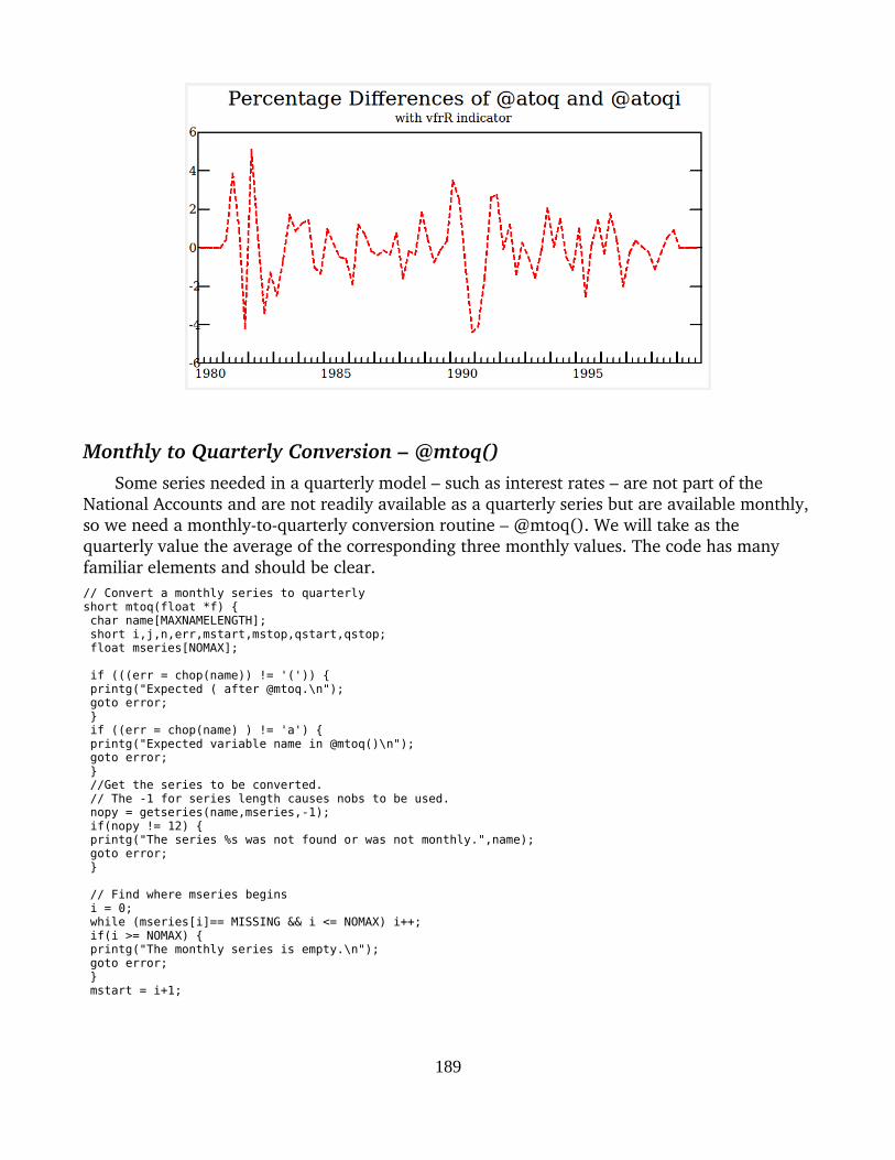
Monthly to Quarterly Conversion – @mtoq()Some series needed in a quarterly model – such as interest rates – are not part of the
National Accounts and are not readily available as a quarterly series but are available monthly,so we need a monthlytoquarterly conversion routine – @mtoq(). We will take as the quarterly value the average of the corresponding three monthly values. The code has many familiar elements and should be clear.// Convert a monthly series to quarterlyshort mtoq(float *f) { char name[MAXNAMELENGTH]; short i,j,n,err,mstart,mstop,qstart,qstop; float mseries[NOMAX];
if (((err = chop(name)) != '(')) { printg("Expected ( after @mtoq.\n"); goto error; } if ((err = chop(name) ) != 'a') { printg("Expected variable name in @mtoq()\n"); goto error; } //Get the series to be converted. // The -1 for series length causes nobs to be used. nopy = getseries(name,mseries,-1); if(nopy != 12) { printg("The series %s was not found or was not monthly.",name); goto error; }
// Find where mseries begins i = 0; while (mseries[i]== MISSING && i <= NOMAX) i++; if(i >= NOMAX) { printg("The monthly series is empty.\n"); goto error; } mstart = i+1;
189
// Find where mseries ends while(mseries[i] != MISSING && i <= NOMAX) i++; mstop = i-1; // and get the corresponding quarterly dates. qstart = mstart/3; qstop = mstop/3; // Average each three monthly values to get the quarterly value, which is returned. for(i = qstart; i <= qstop;i++){ j= i*3; f[i] = (mseries[j]+mseries[j+1]+mseries[j+2])/3.0; }
return OK;
error: return ERR; }
The routine was tested with the following command file with data designed to make checking the results easy:#mtoq test
data mseries 1980m01 3 3 3 4 4 4 5 5 5 6 6 6 7 7 7 8 8 8 9 9 9 10 10 10 9 9 9 8 8 8 7 7 7 6 6 6 7 7 7 6 6 6 5 5 5 4 4 4; tdates 1980m01 1983m12 type mseries
fdates 1980q1 1985q4 f qseries = @mtoq(mseries)
tdates 1980q1 1983q4 type qseries
with these satisfying results:Here is qseries: 1980q1 3.000 4.000 5.000 6.000 1981q1 7.000 8.000 9.000 10.000 1982q1 9.000 8.000 7.000 6.000 1983q1 7.000 6.000 5.000 4.000
G7 has myriad functions, more than anyone can remember, but the ones now written for Gwx should make most quarterly econometric modeling possible. If you need one not here, write it or get in touch.
190
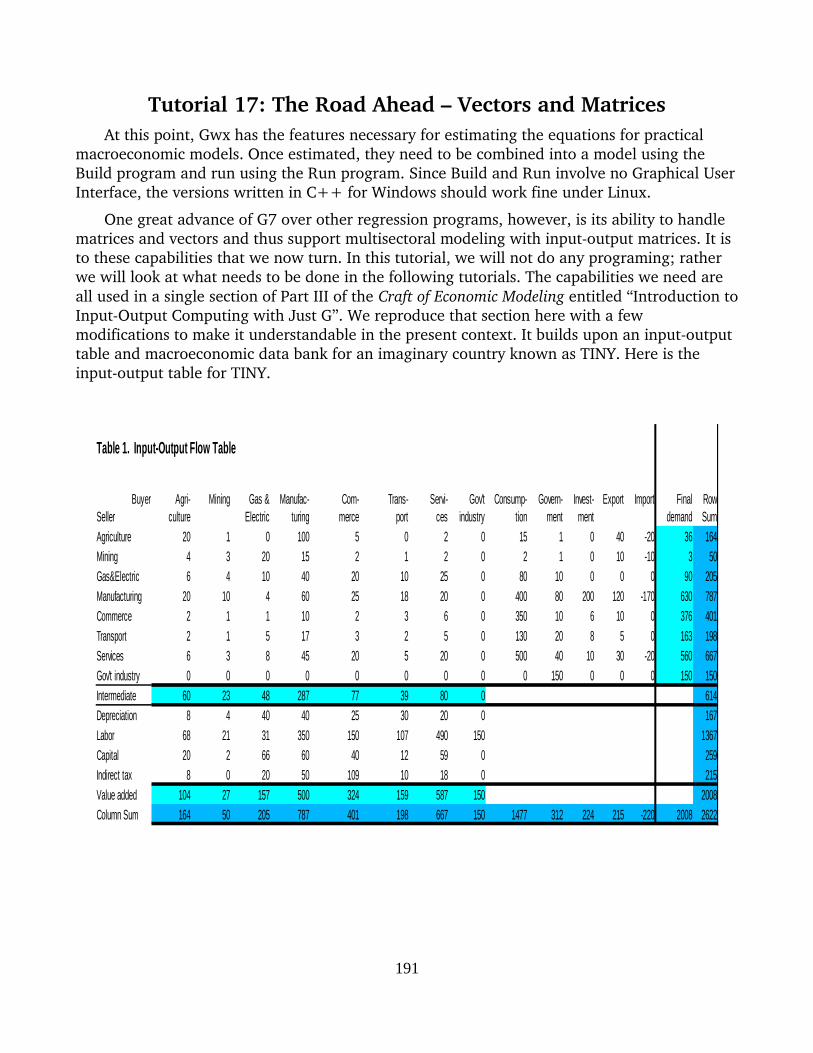
Tutorial 17: The Road Ahead – Vectors and MatricesAt this point, Gwx has the features necessary for estimating the equations for practical
macroeconomic models. Once estimated, they need to be combined into a model using the Build program and run using the Run program. Since Build and Run involve no Graphical UserInterface, the versions written in C++ for Windows should work fine under Linux.
One great advance of G7 over other regression programs, however, is its ability to handle matrices and vectors and thus support multisectoral modeling with inputoutput matrices. It is to these capabilities that we now turn. In this tutorial, we will not do any programing; rather we will look at what needs to be done in the following tutorials. The capabilities we need are all used in a single section of Part III of the Craft of Economic Modeling entitled “Introduction toInputOutput Computing with Just G”. We reproduce that section here with a few modifications to make it understandable in the present context. It builds upon an inputoutput table and macroeconomic data bank for an imaginary country known as TINY. Here is the inputoutput table for TINY.
191
Table 1. Input-Output Flow Table
Buyer Agri- Mining Gas & Manufac- Com- Trans- Servi- Gov't Consump- Govern- Invest- Export Import Final RowSeller culture Electric turing merce port ces industry tion ment ment demand Sum
Agriculture 20 1 0 100 5 0 2 0 15 1 0 40 -20 36 164
Mining 4 3 20 15 2 1 2 0 2 1 0 10 -10 3 50
Gas&Electric 6 4 10 40 20 10 25 0 80 10 0 0 0 90 205
Manufacturing 20 10 4 60 25 18 20 0 400 80 200 120 -170 630 787
Commerce 2 1 1 10 2 3 6 0 350 10 6 10 0 376 401
Transport 2 1 5 17 3 2 5 0 130 20 8 5 0 163 198
Services 6 3 8 45 20 5 20 0 500 40 10 30 -20 560 667
Gov't industry 0 0 0 0 0 0 0 0 0 150 0 0 0 150 150
Intermediate 60 23 48 287 77 39 80 0 614
Depreciation 8 4 40 40 25 30 20 0 167
Labor 68 21 31 350 150 107 490 150 1367
Capital 20 2 66 60 40 12 59 0 259
Indirect tax 8 0 20 50 109 10 18 0 215
Value added 104 27 157 500 324 159 587 150 2008
Column Sum 164 50 205 787 401 198 667 150 1477 312 224 215 -220 2008 2622

What the GOnly Model Will DoWe will see how to turn the TINY inputoutput table and data bank into a simple input
output model using only commands which we will proceed to make available in Gwx. In this model, we will move each final demand column forward and backward over the period 1995 2003 by the index of the corresponding GDP component in the TINY data bank. Then we moveall the final demand vectors except investment up by 3.0 percent per year from 2003 to 2010. Investment is moved forward by a wavy series composed of a base series growing at 3.0 percent per year plus a sinusoidal function. Inputoutput coefficients and the composition of the five final demand components are kept constant. Outputs by each industrial sector are thencalculated for every year from 1995 to 2010. With the additional assumption that the shares ofeach type of income in value added by each industry remain constant, we calculate income of each type in each industry. Linear trends in the inputoutput coefficients, valueadded coefficients, and composition of the final demand vectors could easily be introduced, but that has been left as an exercise.
This model is incomplete and somewhat inconsistent with itself for many reasons, including the following: (a) it does not assure consistency of Personal consumption expenditure with the Personal income it implies (b) it does not relate the imports of a product to the domestic use of the product, and (c) investment is not detailed by industry and related to the growth of the industry as found by the model. Introducing such features to exploit the full potential of inputout modeling requires the nonGUI Interdyme software described in the Craft of Economic Modeling, which works in conjunction with Gwx. Despite these limitations, such simple trailer models, though with greater industry detail and more finely divided final demands, have been widely and shamelessly used by groups which have a macroeconomic model and want industry outputs consistent with its forecasts of aggregate final demand categories.
How To Do Multisectoral Modeling with Just G7Working with inputoutput in G7 requires the use of a new sort of data bank known as a
VAM (Vectors And Matrices) file. As the name suggests, this type of data bank holds time series of vectors and matrices. G has commands which can add, subtract, multiply, and invert matrices and add and subtract vectors and multiply them by matrices. Thus, the operations discussed so far, and several others, can easily be performed in G. A VAM file differs in two important respects from the G data banks we have worked with so far:
(1) In the standard G bank, all elements are the same size, namely a time series of a singlevariable beginning at the beginning of the data bank and extending over the number of observations in the bank, as specified by the G.cfg file. In VAM files, elements are time series ofvectors or matrices of various dimensions. As in the standard G bank, all time series are the same length.
(2) In standard G banks, we can create new series as we work, for example, with f, fex, or data commands. In VAM files, we buy the flexibility of having elements of various sizes by specifying at the outset (in a file usually called VAM.CFG) the contents of the file, that is, the names and dimensions of each vector or matrix in the bank along with the names of the files
192

giving the titles of the row or columns of the vector or matrix. One might suppose that it is a bit of nuisance to have to specify this structure of the VAM file at the outset. In practice, however, this need to prespecify structure proves a useful discipline in building complex models. If, as a model evolves, it becomes necessary to revise the specification of the VAM file, it is easy to copy the contents of the old file into the new, enlarged file, or simply to remake the VAM file.
We can illustrate the use of the VAM file and some new G commands for making some simple calculations with the inputoutput table presented above, which we will assume is for the year 2000. The box below shows the VAM.CFG file for this model, which we will call TINYI.
The first line in VAM.CFG gives the beginning and ending years for the VAM file. The next line, the one beginning with a #, is a comment to clarify the structure of the file. Comments beginning with a # can be placed anywhere in the file. Then come freeform lines giving
1. The name of the element2. Its number of rows 3. Its number of columns4. The maximum number of lags with which a vector occurs in the model5. The name of a file containing the names of the rows of a vector or matrix6. The name of a file containing the names of the columns of a matrix7. A # followed by a brief description of the element.
As far as the computer is concerned, these lines are free format; all that is needed is one ormore spaces between each item on a line. But this is a file also read by humans, so putting in spaces to make the items line up in neat columns is also a good idea. The accompanying box shows the vam.cfg file for the TINY model based on example of section 1 of this chapter.
193

VAM.CFG File for the TINY Model
1995 2010FM 8 8 0 sectors.ttl sectors.ttl #Input-output flow matrixAM 8 8 0 sectors.ttl sectors.ttl #Input-output coefficient matrixLINV 8 8 0 sectors.ttl sectors.ttl # Leontief inverseout 8 1 3 sectors.ttl # Outputpce 8 1 0 sectors.ttl # Personal consumption expendituregov 8 1 0 sectors.ttl # Government spendinginv 8 1 0 sectors.ttl # Investmentex 8 1 0 sectors.ttl # Exportsim 8 1 0 sectors.ttl # Importsfd 8 1 0 sectors.ttl # Total final demanddep 8 1 0 sectors.ttl # Depreciationlab 8 1 0 sectors.ttl # Labor incomecap 8 1 0 sectors.ttl # Capital incomeind 8 1 0 sectors.ttl # Indirect taxesdepc 8 1 0 sectors.ttl # Depreciation coefficientslabc 8 1 0 sectors.ttl # Labor income coefficientscapc 8 1 0 sectors.ttl # Capital income coefficientsindc 8 1 0 sectors.ttl # Indirect taxes coefficientspcec 8 1 0 sectors.ttl # Personal consumption sharesinvc 8 1 0 sectors.ttl # Investment sharesgovc 8 1 0 sectors.ttl # Gov sharesexc 8 1 0 sectors.ttl # Export sharesimc 8 1 0 sectors.ttl # Import sharesx 8 1 0 sectors.ttl # Working spacey 8 1 0 sectors.ttl # Working space
To create a vam file from a vam configuration file the command in G7 is – and in Gwx willbe –
vamcreate <vam configuration file> <vam file>
For example, to create the vam file HIST.VAM from the configuration file VAM.CFG, the command is
vamcreate vam.cfg hist
The vamcreate command may be abbreviated to vamcr, thus:vamcr vam.cfg hist
At this point, the newly created vam file has zeros for all its data. We will now see how to put data into it and work with that data. The first step is to assign it as a bank. The command is
vam <filename> <letter name of bank>
For example,vam hist b
will assign HIST.VAM as bank b. Letters a through v may be used to designate banks. However, it is generally a good practice to leave a as the G bank which was initially assigned.
194
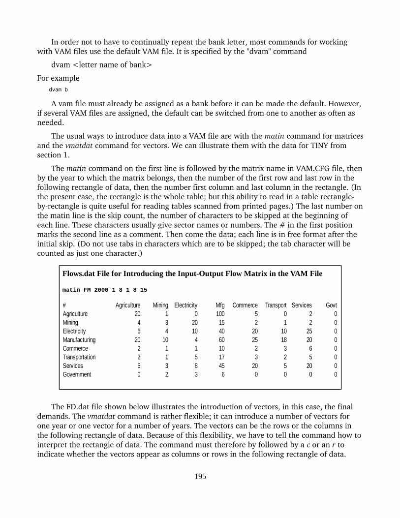
In order not to have to continually repeat the bank letter, most commands for working with VAM files use the default VAM file. It is specified by the "dvam" command
dvam <letter name of bank>
For exampledvam b
A vam file must already be assigned as a bank before it can be made the default. However,if several VAM files are assigned, the default can be switched from one to another as often as needed.
The usual ways to introduce data into a VAM file are with the matin command for matricesand the vmatdat command for vectors. We can illustrate them with the data for TINY from section 1.
The matin command on the first line is followed by the matrix name in VAM.CFG file, thenby the year to which the matrix belongs, then the number of the first row and last row in the following rectangle of data, then the number first column and last column in the rectangle. (Inthe present case, the rectangle is the whole table; but this ability to read in a table rectanglebyrectangle is quite useful for reading tables scanned from printed pages.) The last number onthe matin line is the skip count, the number of characters to be skipped at the beginning of each line. These characters usually give sector names or numbers. The # in the first position marks the second line as a comment. Then come the data; each line is in free format after the initial skip. (Do not use tabs in characters which are to be skipped; the tab character will be counted as just one character.)
Flows.dat File for Introducing the Input-Output Flow Matrix in the VAM File
matin FM 2000 1 8 1 8 15
The FD.dat file shown below illustrates the introduction of vectors, in this case, the final demands. The vmatdat command is rather flexible; it can introduce a number of vectors for one year or one vector for a number of years. The vectors can be the rows or the columns in the following rectangle of data. Because of this flexibility, we have to tell the command how tointerpret the rectangle of data. The command must therefore by followed by a c or an r to indicate whether the vectors appear as columns or rows in the following rectangle of data.
195
# Agriculture Mining Electricity Mfg Commerce Transport Services GovtAgriculture 20 1 0 100 5 0 2 0Mining 4 3 20 15 2 1 2 0Electricity 6 4 10 40 20 10 25 0Manufacturing 20 10 4 60 25 18 20 0Commerce 2 1 1 10 2 3 6 0Transportation 2 1 5 17 3 2 5 0Services 6 3 8 45 20 5 20 0Government 0 2 3 6 0 0 0 0

Here, the vectors are clearly columns. The next number is the number of vectors in the rectangle; here 5. Next is the number of years represented in the rectangle. Here it is 1, for thecolumns are different vectors for the same year. (Either the number of vectors or the number of years must be 1.) The next two numbers are the first and last element numbers of the data in the rectangle, and the last is the skip count as before. Since this command is introducing several vectors for one year, that year is specified at the beginning of the next line, and the names of the vectors follow it. (If we were introducing data for one vector for several years, the vector name would be in the first position on this line, followed by the year numbers.)
The FD.dat File for Introducing the Final Demands into the VAM File
vmatdata c 5 1 1 8 152000 pce gov inv ex im# PersCon Gov Invest Exports ImportsAgriculture 15 1 0 40 -20Mining 2 1 0 10 -10Electricity 80 10 0 0 0Manufacturing 400 80 200 120 -170Commerce 350 10 6 10 0Transportation 130 20 8 5 0Services 500 40 10 30 -20Government 0 150 0 0 0
The valueadded rows are introduced by the vmatdat command and data shown in the boxbelow.
The VA.dat File for Introducing the Value-Added Vectors
vmatdata r 4 1 1 8 152000 dep lab cap ind# 1 2 3 4 5 6 7 8Depreciation 8 4 40 40 25 30 20 0Labor 68 21 31 350 150 107 490 150Capital 20 2 66 60 40 12 59 0Indirect tax 8 0 20 50 109 10 18 0
Here, finally, are the G commands to create the VAM file and load the data into it:
# Create and load the VAM file for TINYvamcreate vam.cfg histvam hist bdvam b# Bring in the intermediate flow matrixadd flows.dat# Bring in the final demand vectorsadd fd.dat# Bring in the value added vectorsadd va.dat
196
These and the following commands to G for making the calculations described in this section are in the file GMODEL.PRE shown on page 198. To fit this large file on a single page, some commands have been doubled up on a single line but separated by a semicolon – a trick which works in G as in C++.
Now let us look at some of the data we have introduced by displaying them in a grid on the screen. The command
show FM y 2000
will show in a spreadsheetlike grid the FM matrix, the flow matrix for the year 2000. To adjust the default column width and the number of decimal places in the display, click the Options menu item. Not only does this display look like a spreadsheet display, it also works like one in that you can copy and paste between data from one to the other.
To look at a row, say row 2, of the FM matrix for all years of the VAM file, the command isshow FM r 2
while to show column 5 for all years, the command isshow FM c 5
Thus, in showing a matrix, we have to choose among showing the whole matrix for one year and showing one row or column for all years. The choice is indicated by the letter – a y, r or c – following the matrix name.
Showing vectors is simpler because we do not have to make this choice; we just name the vector and get all values for all years. Here are two examples
show ind # Display the indirect tax vectorshow b.pce # Display the personal consumption expenditure vector
The second of these examples shows that the show command allows us to specify by the bank letter followed by a dot the bank from which the item is to be shown.
Now that we have read in the data and displayed it to check that it was accurately read, we can begin to compute. To calculate the inputoutput coefficient matrix, we need out, the vector of outputs by industry. It was not read in, but it can be computed by summing the rows of the FM matrix and then adding to this row sum the final demand columns. Here are the twocommands and the show command to see the result:
# Add up the intermediate rows getsum FM r out# Add on the final demand vectors to get total outputvc out = out+pce+gov+inv+ex+imshow b.out
We are now ready to copy the flow matrix, stored in FM, to AM and then convert it to inputoutput coefficients by dividing each element of each column by the corresponding element of the out vector. We do the copy with the with the mcopy command, for “matrix copy.” The general form of the mcopy command to copy matrix or vector A from bank x to element B in bank y is
mcopy y.B [=] x.A
197
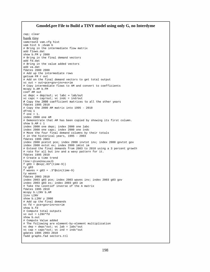
Gmodel.pre File to Build a TINY model using only G, no Interdyme
zap; clear
bank tinyvamcreate vam.cfg histvam hist b ;dvam b# Bring in the intermediate flow matrixadd flows.datshow b.FM y 2000# Bring in the final demand vectorsadd fd.dat# Bring in the value added vectorsadd va.datfdates 2000 2000# Add up the intermediate rows getsum FM r out# Add on the final demand vectors to get total outputvc out = out+pce+gov+inv+ex+im# Copy intermediate flows to AM and convert to coefficientsmcopy b.AM b.FMcoef AM outvc depc = dep/out; vc labc = lab/outvc capc = cap/out; vc indc = ind/out# Copy the 2000 coefficient matrices to all the other yearsfdates 1995 2010# Copy the 2000 AM matrix into 1995 - 2010dfreq 1f one = 1.index 2000 one AM# Demonstrate that AM has been copied by showing its first column.show b.AM c 1index 2000 one depc; index 2000 one labcindex 2000 one capc; index 2000 one indc# Move the four final demand columns by their totals# in the historical years, 1995 - 2003fdates 1995 2003index 2000 pcetot pce; index 2000 invtot inv; index 2000 govtot govindex 2000 extot ex; index 2000 imtot im# Extend the final demands from 2003 to 2010 using a 3 percent growth# rate for all but inv and a wavy pattern for it.fdates 1995 2010# Create a time trendf time = @cum(time,one,0)f g03 = @exp(.03*(time-9))ty g03f waves = g03 + .3*@sin(time-9)ty wavesfdates 2003 2010index 2003 g03 pce; index 2003 waves inv; index 2003 g03 govindex 2003 g03 ex; index 2003 g03 im# Take the Leontief inverse of the A matrixfdates 1995 2010mcopy b.LINV b.AMlinv LINVshow b.LINV y 2000# Add up the final demandsvc fd = pce+gov+inv+ex+imshow b.fd# Compute total outputsvc out = LINV*fdshow b.out# Compute Value added# The following are element-by-element multiplicationvc dep = depc*out; vc lab = labc*outvc cap = capc*out; vc ind = indc*outgdates 1995 2003 2010fadd graphs.fad sectors.ttl
198

The = sign is optional but is a useful reminder of which way the copy is going. The y. is optional if y is the default VAM file, and the same is true for the x.. Since this copy and these calculations need be done only for one year, the first, 2000, we first set the fdates so that the mcopy and coef commands work only on the years from 2000 to 2000 (which is to say, only for2000). Here are the commands
# Copy intermediate flows to AM and convert to coefficientsfdates 2000 2000mcopy b.AM = b.FMcoef AM outshow AM y 2000# Create value-added coefficient vectors.vc depc = dep/outvc labc = lab/outvc capc = cap/outvc indc = ind/out# Set fdates back to the entire range of the VAM file.fdates 1995 2010
With the inputoutput coefficients calculated, we can now go on to illustrate finding the Leontief inverse, calculating outputs from exogenous forecasts of final demands, calculating valueadded components, and displaying, graphing, and making tables of the results. We will first copy the inputoutput coefficient matrix and the valueadded coefficient vectors from 1995 to the other years out to 2010. We can conveniently do this with G’s index command. This command is used to move all elements of a vector or matrix in the default VAM file forward or backward in proportion to a guide series. Its general form is:
index <base year> <guide series> <matrix or vector>
It operates over the range specified by the current value of the fdates. Since we just want to copy the coefficients to all the years, our guide series will be simply a series of 1's, which we shall call one. Here are the commands
# Copy the 2000 AM matrix into 1995 - 2010dfreq 1f one = 1.index 2000 one AMindex 2000 one depcindex 2000 one labcindex 2000 one capcindex 2000 one indcshow AM c 1
The last command displays in a grid the first column of the AM matrix for all the years; all columns of this display should, of course, be identical. For purposes of our illustration, we will let AM remain constant in all years.
The final demands, however, we will move in a slightly more interesting way. Between 1995 and 2003, each the elements of each final demand column will follow the index of the total of that column as given in the national accounts. Here are the G commands to make that happen.
# Move the four final demand columns by their totals# in the historical years, 1995 - 2003fdates 1995 2003index 2000 pcetot pceindex 2000 invtot invindex 2000 govtot govindex 2000 extot ex
199
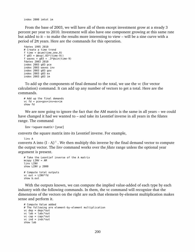
index 2000 imtot im
From the base of 2003, we will have all of them except investment grow at a steady 3 percent per year to 2010. Investment will also have one component growing at this same rate but added to it – to make the results more interesting to view – will be a sine curve with a period of 2 years. Here are the commands for this operation. π
fdates 1995 2010# Create a time trendf time = @cum(time,one,0)f g03 = @exp(.03*(time-9))f waves = g03 + .3*@sin(time-9)fdates 2003 2010index 2003 g03 pce index 2003 waves invindex 2003 g03 govindex 2003 g03 exindex 2003 g03 im
To add up the components of final demand to the total, we use the vc (for vector calculation) command. It can add up any number of vectors to get a total. Here are the commands.
# Add up the final demandsvc fd = pce+gov+inv+ex+imshow fd
We are now going to ignore the fact that the AM matrix is the same in all years – we could have changed it had we wanted to – and take its Leontief inverse in all years in the fdates range. The command
linv <square matrix> [year]
converts the square matrix into its Leontief inverse. For example,linv A
converts A into (I A)1 . We then multiply this inverse by the final demand vector to compute the output vector. The linv command works over the fdate range unless the optional year argument is present.
# Take the Leontief inverse of the A matrixmcopy LINV = AMlinv LINVshow LINV y 2000
# Compute total outputsvc out = LINV*fdshow b.out
With the outputs known, we can compute the implied valueadded of each type by each industry with the following commands. In them, the vc command will recognize that the dimensions of the vectors on the right are such that elementbyelement multiplication makes sense and perform it.
# Compute Value added# The following are element-by-element multiplicationvc dep = depc*outvc lab = labc*outvc cap = capc*outvc ind = indc*outshow lab
200

As we went along, we showed results in spreadsheetlike grids to check that our answers were generally reasonable. Now we need to graph the results. In doing so, we use the fact that elements of vectors in a VAM file can be referred to in G simply by the name of the vector followed by a numeral. We can graph the second element of the out and pce vectors from the VAM file assigned as bank b with the graph command like this:
gr b.out2 b.pce2
If the VAM file is the default VAM file, we can omit the bank letter and period. Thus, in theinstance just given, we could do just
gr out2 pce2
This way of working with a time series of elements of a vector works also for type and r commands and for the righthand side of f or fex commands. Similarly, we can refer to an element of a matrix in a type, graph, or r command or the right side of an f command by the matrix name followed by the row number, followed by a dot, followed by the column number. For example,
type AM3.5
will print to the screen the values of the element in the third row and fifth column of the AM matrix.
We can get a lot more graphs very quickly by use of G’s fadd command. The name fadd is acontraction of “filedirected add command.” It works with text substitution in a way that is very convenient in working with multisectoral models. The general form is
fadd <command file> <argument file>
In our case, the “command file” will be the following file, named GRAPHS.FAD:vr 0ti %3 %5subti Output and Final demandgname out%3gr b.out%3 b.fd%3subti Depreciation,Labor income, Capital income, Indirect taxesgname va%3gr b.dep%3 b.lab%3 b.cap%3 b.ind%3tisubti
and the argument file will be the same SECTORS.TTL file which we used for supplying row and column names for the matrices and vectors in the VAM file, namely:
Agricul ;1 e "Agriculture"Mining ;2 e "Mining and quarrying"Elect ;3 e "Electricity and gas"Mfg ;4 e "Manufacturing"Commerce ;5 e "Commerce"Transport ;6 e "Transportation"Services ;7 e "Services"Government ;8 e "Government"
Note that some of the lines in the command file – for example, the second – have a %
201

followed by a number. These numbers refer to “arguments” from the “argument” file. For example, on the first line of the argument file, argument 1 is Agricul, argument 2 is ;, argument 3 is 1, argument 4 is e , and argument 5 is Agriculture . Normally an argument is ended by a space or punctuation. Enclose arguments which contain spaces – such as the namesof some sectors – in quotation marks. When the second line of the command file,
ti %3 %5
is executed with the arguments 3 and 5 from the first line of the argument file replacing the %3 and %5, the effect is that G executes the command
ti 1 Agriculture
The effect of the fadd command is that the entire command file is executed first with arguments from the first line of the argument file, then with the arguments from the second line of the argument file, and so on. Thus, with the single command
fadd graphs.fad sectors.ttl
G will draw for all sectors graphs like the two shown below for Manufacturing.
We have used some but not all of the G commands for matrix arithmetic in a VAM file. Forreference, here are some others.
minv A converts A into its inverse
madd A = B + C adds B and C and stores the result in A
madd A = B C subtracts C from B and stores the result in A
mmult A = B*C multiplies B and C and stores the result in A
mmult A = B’C multiplies B transpose by C and stores the result in A
mmult A = B&C does elementbyelement multiplication of B and C and stores the result in A
mmult A = B/C elementbyelement division of B by C stored in A
mtrans A B the transpose of B is stored in A
In all of them, the command may be followed by an optional year in which to do the calculation; absent the year, the calculation is done for all years in the fdates range.
Here ends the quotation from The Craft of Economic Modelling.
So What Needs to be Written?By looking back over the preceding section, we see that we need to write the following
commands:
vamcreate – to create a VAM file from a vam.cfg file.
202

vam – to assign a vam file to a bank letter, a through v.
dvam – to make one vam file the default for the commands to follow.
matin – to read a matrix from a text file into a VAM file.
show – to display in a grid a matrix for one year or a vector or row or column of a matrix for several years.
vmatdat – to read vectors from a text file into a VAM file.
getsum – to sum the rows or columns of a matrix.
vc – vector calculations, to add or subtract vectors, and perform other vector computations.
mcopy – copy one matrix to another.
linv – form the Leontief inverse of a matrix.
coef – form an inputoutput coefficient matrix from a flow matrix and a vector of outputs.
index – multiply a matrix for one year by a scalar and copy the product to other years.
fadd – the filedirected “add” command.
minv – take the inverse of a matrix.
madd – add two matrices.
mmult – multiply two matrices in various ways (as in matrix algebra, or elementbyelement, or after first transposing the first, or by dividing elementbyelement).
mtrans – transpose a matrix.
extensions to gr and type commands for elements of vectors.
All but one of these commands is just algebraic programming, and it should be possible to borrow code from G7. Such borrowing, however, is not always easy because the original coding in G7 has been overlaid by many changes, some useful but many without evident purpose.
The one command that is not algebraic programing but requires working with the graphical user interface is the show command which displays on the screen in a rectangular grid either a matrix for single year or a time series of values for a vector or for one row or one column of a matrix. For the grid display we must use the last and most complicated wxWidget we shall need, the wxGrid. Learning to use wxGrid from the Smart and Hock book is impossible; far too little is explained and some of what is explained is highly misleading if not plain wrong. Fortunately, wxSmith knows how to use wxGrid and can teach us most of what we need to know. One whole tutorial will be devoted just to a demonstration of the use wxGrid and then another to the show() command. First, however, we need to create a VAM file.
203
Tutorial 18. Creating a VAM File
VAM Files from the User's ViewpointWe will deal next with the databanks known as VAM files which contain not time series on
single variables but time series of vectors and matrices, from which the name VAM comes. The basics of the use of VAM files is explained in the first chapter of Part 3 of The Craft of EconomicModeling. In this tutorial, we will deal only with the creation of an empty VAM file from the information in a vam.cfg file. In other words, we will build the framework for holding the data;but we will not put any data into that structure nor assign it as a data bank into which data can be put or from which data can be drawn. Assigning it as a data bank is the subject of Tutorial 18; putting in data comes in Tutorial 19; and displaying it comes in Tutorial 20. Further tutorials will then deal with working with the data.
First, a word of review on the two fundamental differences between a VAM file and the G data banks we have worked with so far:
(1) In the standard G bank, all elements are the same size, namely a time series of a singlevariable beginning at the beginning of the data bank and extending over the number of observations in the bank, as specified by the G.cfg file. In VAM files, elements are time series ofvectors or matrices of various dimensions. As in the standard G bank, all time series are the same length, although data may be missing for some periods for some vectors or matrices.
(2) In standard G banks, we can create new series as we work, for example, with f, fex, or data commands. In VAM files, we buy the flexibility of having elements of various sizes by specifying at the outset (in a file usually called VAM.CFG) the contents of the file, that is, the names and dimensions of each vector or matrix in the bank along with the names of the files giving the titles of the row or columns of the vector or matrix. One might suppose that it is a bit of nuisance to have to specify this structure of the VAM file at the outset. In practice, however, this need to prespecify structure proves a useful discipline in building complex models. If, as a model evolves, it becomes necessary to revise the specification of the VAM file, it is easy use the command prompt program vam2vam to copy the contents of the old file into the new, enlarged file, or simply to remake the VAM file.*
To make a new, empty (but structured) VAM file, the user gives Gwx the command
vamcreate <InputFile> <OutputFile>
where <InputFile> is the name of a VAM configuration file, often simply VAM.CFG, and <OutputFile> is the name of the VAM file to be created. For example,
vamcreate vam.cfg tiny.vam
* In G7 for Windows, a lot of intricate coding is connected with packed matrices. In input-output work, there often occur large matrices with only a few non-zero elements. To handle models with such matrices in the computers of the 1990's, itwas worthwhile to write algorithms to store only the non-zero elements of such matrices and to work with them in that form. By 2015, even the largest input-output matrices were small in comparison with the capacities of even the most basic computers. Consequently, packed matrices have largely fallen out of use, and I have no intention of including themin Gwx.
204
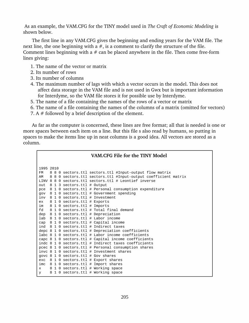
As an example, the VAM.CFG for the TINY model used in The Craft of Economic Modeling is shown below.
The first line in any VAM.CFG gives the beginning and ending years for the VAM file. The next line, the one beginning with a #, is a comment to clarify the structure of the file. Comment lines beginning with a # can be placed anywhere in the file. Then come freeform lines giving:
1. The name of the vector or matrix2. Its number of rows 3. Its number of columns4. The maximum number of lags with which a vector occurs in the model. This does not
affect data storage in the VAM file and is not used in Gwx but is important information for Interdyme, so the VAM file stores it for possible use by Interdyme.
5. The name of a file containing the names of the rows of a vector or matrix6. The name of a file containing the names of the columns of a matrix (omitted for vectors)7. A # followed by a brief description of the element.
As far as the computer is concerned, these lines are free format; all that is needed is one ormore spaces between each item on a line. But this file s also read by humans, so putting in spaces to make the items line up in neat columns is a good idea. All vectors are stored as a column.
VAM.CFG File for the TINY Model
1995 2010FM 8 8 0 sectors.ttl sectors.ttl #Input-output flow matrixAM 8 8 0 sectors.ttl sectors.ttl #Input-output coefficient matrixLINV 8 8 0 sectors.ttl sectors.ttl # Leontief inverseout 8 1 3 sectors.ttl # Outputpce 8 1 0 sectors.ttl # Personal consumption expendituregov 8 1 0 sectors.ttl # Government spendinginv 8 1 0 sectors.ttl # Investmentex 8 1 0 sectors.ttl # Exportsim 8 1 0 sectors.ttl # Importsfd 8 1 0 sectors.ttl # Total final demanddep 8 1 0 sectors.ttl # Depreciationlab 8 1 0 sectors.ttl # Labor incomecap 8 1 0 sectors.ttl # Capital incomeind 8 1 0 sectors.ttl # Indirect taxesdepc 8 1 0 sectors.ttl # Depreciation coefficientslabc 8 1 0 sectors.ttl # Labor income coefficientscapc 8 1 0 sectors.ttl # Capital income coefficientsindc 8 1 0 sectors.ttl # Indirect taxes coefficientspcec 8 1 0 sectors.ttl # Personal consumption sharesinvc 8 1 0 sectors.ttl # Investment sharesgovc 8 1 0 sectors.ttl # Gov sharesexc 8 1 0 sectors.ttl # Export sharesimc 8 1 0 sectors.ttl # Import sharesx 8 1 0 sectors.ttl # Working spacey 8 1 0 sectors.ttl # Working space
205

If we think of the data in the vam.cfg as a matrix with each line of the vam.cfg file as a row, then the VAM file contains, after an introductory summary description, the transpose of that matrix. There is one long vector with all the array names, then a vector with the number of rows of each array, then vector with the number columns, and so on. After this “transpose” of the vam.cfg file comes the data for the first array in the first year, then the data for the second array in the first year, on through the last array in the first year. After that comes the data for the second year in the same order. Then follows the data for the third year and so on up to the last year.
It is the job of the vamcreate command to read the vam.cfg file, make up and write the summary description, then write this transposed form of the vam.cfg file, and then write data for all the arrays, year by year. The data written, however, is all zeros.
In designing the VAM file there was a choice between (a) having all the data for year 1 followed by all the data for year 2, followed by all the data for year 3, etc. or (b) having all thedata for array 1, followed by all the data for array 2, followed by all the data for year 3, etc. My choice of option (a) was perhaps unduly influenced by experience with the Univac 1108, where the Fortran compiler had a function called NTRAN which could read in rapidly a large amount of contiguous data. It was my idea to read in all of the data for one year in one big gulp. I never found a way to do that in C++. The vectors and matrices are each read one by one. Whether or not the fact that each year's data was originally written as one long vector of zeros by vamcreate makes for fast reading I do not know. Some experimenting might be interesting. The downside of my choice is that whenever – in the course of model development– an array has to be added to the VAM file, a whole new file must be created and data from the old VAM file copied to it by use of the command line program vam2vam.
The vamcreate command may be abbreviated to vamcr, thus:vamcr vam.cfg hist.vam
At this point, the newly created vam file has, as already mentioned, zeros (or more correctly, MISSINGs) for all its data.
Writing the vamcreate command is the sole subject of this tutorial.
Two Preliminaries: gstrcpy() and stringer()The vamcreate function will clearly have to read the VAM configuration file just described.
Since this file is a text file, it seemed natural to read it a line at a time using the standard C library function fscanf() to get the various items from the line. I was aware that in the past fscanf() sometimes gave trouble, but I thought that perhaps it had been fixed and was now usable. Indeed, it seemed to read the fields correctly, but then the program would soon crash. Close study with the debugger revealed that fscanf() was changing the values of other variables not even involved in the call to fscanf(). An alternative to fscanf() had to be found. In G7, our old friend chop() was directed to take input from the VAM configuration file. This is a somewhat delicate operation, and I decided on a more transparent alternative. The following simple program, stringer(), starts reading a given string (source) at a specified byte (start), skips any white space, then copies characters into a second string (found) until a blank or end
206

ofline is encountered. It then puts a null at the end of found, and returns the number of the blank or endofline character that stopped the reading from source. /* Pull space-separated segments from a longer string. source is the longer string; start is the byte number in source where we start looking for a segment; found is the substring we want. found should have space for 40 or more bytes. The byte number of the byte that stopped the segment is returned.*/short stringer(char *source, short start, char *found){
short i,j; i = start; j = 0; while(source[i] == ' ') i++; while(source[i] != ' ' && source[i] != '\n' && j < 40){ found[j++] = source[i++];
} found[j] = '\0'; return i; }
The found string can then be put through the atoi() function to get an integer from the ascii string returned by stringer(). We will soon see examples of its use.
For copying the vector and matrix names into one long array with just a NULL between them, we will use the simple but useful gstrcpy() function which is found in utility.cpp. Here isthe code./***********************************************************************//* gstrcpy(target,source) - the value returned is the pointer to the next free space in the target *//***********************************************************************/char *gstrcpy(char *target, char *source){
while((*target++ = *source++)!= 0); return(target); }
The VamFileDesc structEvery VAM file begins with 102 bytes of information about the file, called the File
Description. They are organized into a C++ struct as follows:struct VamFileDesc { float startdate; // e.g. 1990.
float enddate; // e.g. 2030.int nnpy; // number of numbers per year int startpsn; // position in output file of first element of first vector in first year. short nvecs; // number of vectors and matricesunsigned short ncivnames; //total number of characters in all vector and matrix names short pmcount; // packed matrix count; always 0 in Gwxchar runname[80]; // A description of the contents};
The file description begins with the starting and ending dates of the data in the VAM file. These are, more precisely, the year number of the earliest possible and latest possible data in the VAM file. Were we starting from scratch today and had no need for backward compatibility, the startdate and enddate would be Gdates, but a float is perfectly adequate for annual dates. I know of no use of G with matrices of greater than annual frequency, so there seems to be no reason to loose compatibility with G7 by switching to Gdates.
The number of numbers per year, nnpy, is the total number of floating point numbers in each year's data. For example, if we had two 10x10 matrices and five 10x1 vectors each year,
207

nnpy would be 250 = 2*100 + 5*10.
The next item in the file description, startpsn, requires a word of explanation. Before the actual numerical values for the elements of the vectors and matrices in the VAM file there comes a lot of other information including the file description struct, the names of all these vectors and matrices, the number of rows and columns in each, and the names of the files holding the names of the rows and columns of each matrix. Finally, in byte number startpsn the numerical values of the elements of the matrices and vectors begins.
The next item in the file description is nvecs, the number of vectors and matrices in the VAM file. In the example above, it is 26. The next item, ncivnames, is the number of characters in names of all the matrices and vectors. This count includes the NULL at the end of each name. The packed matrix count, pmcount, will always be 0 in Gwx, but we will retain it in the file description to maintain compatibility with G7 for Windows.
The final item in the file description, runname, is a descriptive title assigned by the user. It may have up to 79 characters plus a NULL (\0) termination. Examples might be “U.S. 65sector tables, historical data” or “Optimistic forecast 2015 2025” or “Stock Market Crash”.
Next in the VAM file, following the file description, comes the array vindx. What is this vindx? The names of the vectors and matrices are going to be written as one long array of characters, vnames, separated by the \0 (or NULL) character, just as in writing the names of the variables in a standard Gbank. The number of the first byte of the name of vector (or matrix) number n is recorded in position n of the vector vindx of unsigned shorts. The count starts from 0.
Next in the VAM file comes the array rows of shorts which holds the number of rows of each vector or matrix, (in the order in which they appear in the vam.cfg file.) Then follows thearray columns which holds the number of columns of each vector or matrix. (Vectors are always considered to be columns and to have 1 as the number of columns.) Next comes the array lags which holds the lags field from the vam.cfg file. Then comes the array of characters types, one character for each vector or matrix, which has v for a vector, m for a matrix, and l for a vector used with one or more lags. At last we get to vnames, the long array of the nullterminated names of the vectors and matrices.
Finally, rowstub and colstub are arrays holding the filenames of the files holding the titles of the rows and columns, respectively, of each array in the VamFile. Space for up to 30 characters in each filename is provided.*
All of this information can be found in (or computed from) the vam.cfg file. All we have todo in the vamcreate command is to read the vam.cfg file, store the information properly, compute vindx and nnpy, write it all out again in the required order into a binary file, and thenappend to this file enough zeros to represent all the vectors and matrices in all the years.
* The word stub seems to require explanation for non-native English speakers. I have been told that some dictionaries give it definitions which can be translated as “a broken tooth, the remaining part of an amputated arm or leg, the end of asmoked cigarette” – all of which is perfectly correct. But there is also another use. In some check books, the check is on right side of the page and a record is on the left. When the check is torn off, the remaining record is the stub. In a table ofdata, the names of the lines, generally on the left of the table, is also called the stub. That is the sense in which it is used here.
208
Notice that vamcreate does not assign as a databank the VamFile it has created; that is the work of a different command, vam, to be covered in the next tutorial. There is therefore no need to make vamcreate a member of the VAMBank class, to be derived from the DataBank class.
The vamcreate CodeWe will write a lot of code related to Vamfiles, so we shall add a new module,
VAMfile.cpp, to Gwx. See page 58 for a review of how to add a module. The module begins// VAMFile.cpp#include <string>#include <iostream>using namespace std;#pragma pack(2)#include "common.h"#include "VamFile.h"
There are two new elements here, the #pragma pack(2) and VamFile.h. The line
#pragma pack(2)
is a compiler directive, an order to the g++ compiler which – on 64bit systems – will make it use 2 bytes for a short, 4 bytes for an int or float and 8 bytes for a long when writing or calculating the size of a struct – such as VamFileDesc. Without the pragma, they would all be written and counted as 8 bytes each. This is a change from 32bit systems, where a long was 4 bytes. The two variables here declared as int were declared as long in G7 for 32bit Windows systems. To maintain compatibility of VAM files created on the two systems, the longs had to be changed to ints. (That wee bit of information cost me about two days of frustration.) There is now said to be available or soon to be available a header file, stdint.h, which has a new set of types for integers with names that include the number of bytes in each type. Its use should make code more portable between systems, but I have not been able to learn how to use it. The pragma, by the way, may be different for different C++ compilers.
In common.h, we have added the lines:#define NVECMAX 300 //Maximum number of vectors and matrices in a VAM file#define MAXCHARINVECNAMES 60000 // Maximum number of characters in vector and matrix names
and// In VAMFile.cppshort vamcreate();short dvam();
The VamFile.h file begins with the struct VamFileDesc shown above and then continues with the definition of the VamFile class which will not concern us until the next tutorial, but here it is for the record:
class VamFile : public DataBank {public: // Constructor that opens an existing .vam file VamFile(const char *rootname);protected:
VamFileDesc fd;unsigned short *vindx;
209

short nobs; // Number of observationsunsigned short *columns,*rows;/*Space for "nvecs" elements of these arrays will be
allocated and they will hold the number of rows and columns of each array (vectoror matrix) in the VAM file. */
unsigned int *sizes, *csizes; /*Space for "nvecs" elements of these arrays will beallocated and they will hold the sizes of each array and the cumulated sizes,respectively.*/
short *lags; /* Space for "nvecs" elements will be allocated, and the numbers in the "lags" columnof the vam.cfg file will be stored there. */
char *vnames; /* up to NCMAX ? */char **rowstub; // filenames for titles of the rows of each vector or matrix.char **colstub; // filenames for titles of the columns of each matrix.char *types; // m for matrices, v for vectors with no lag, l for vectors with lag.
// This is enough to start with; it will grow.};
The vamcreate() program then begins by opening the input and output files:short vamcreate(){
short i, nvecs; char name[40],vamcfgfile[80], vamfilename[80], rownames[40], colnames[40], card[101], sub[40]; char *pvnames; //pointer to vector names unsigned short *columns, *rows,*vindx; short row, col, lag, np; short *lags; char *types,*vnames, **rowstub, **colstub; unsigned int nnpy,*sizes; // int is 4 bytes on 64 bit systems float *x; //to hold the zeroes to be written. FILE *fpc = NULL,*fpout = NULL;
VamFileDesc fd;
// vamcfgfile is the name of the vam.cfg file, input to this commandif(chop(vamcfgfile) != 'a'){
printg("Usage: vamcr <NameOfInput>.cfg> <NameOfOutputk>.vam\n"); printg("Be sure to use the .cfg and .vam.\n");
return(ERR);}
// vamfilename is the name of the .vam file to be createdif(chop(vamfilename) != 'a'){
printg("Usage2: vamcr <name of .cfg file> <name of bank>\n");return(ERR);}
printg("Read both filenames.\n");
// Open the input file for reading text (rt)if((fpc = fopen(vamcfgfile,"rt")) == 0){
printg("Could not open %s.\n",vamcfgfile);return(ERR);}
printg("Opened %s.\n", vamcfgfile);
// Open the output file for writing binary (wb) information.if((fpout = fopen(vamfilename,"wb")) == 0){
printg("Could not open %s.\n",vamfilename); fclose(fpc); return(ERR);
}
printg("Opened both input and output files.\n");
Next, we claim memory sufficient to hold the information we will read from the vam.cfg input file. Since it is hard to imagine that a modern computer would not have space enough for this allocation, we are going to live slightly dangerously and not check that each allocation
210

has been successful.// Allocate space for what will be read from the vam.cfg file
vnames = new char [MAXCHARINVECNAMES]; vindx = new unsigned short [NVECMAX]; sizes = new unsigned int [NVECMAX]; rows = new unsigned short [NVECMAX];
columns = new unsigned short [NVECMAX];lags = new short [NVECMAX];types = new char [NVECMAX];rowstub = new char *[NVECMAX];colstub = new char *[NVECMAX];
Now we need to read the starting and ending dates of the VAM file. Before these dates, however, there may be some comment lines beginning with a # or just a spacer line beginning with the \r character. We need to read past them. I allowed for up to 5 such lines before complaining. Here and throughout this function, we will use the array card to hold a line of input – a choice of words which reflects the programmer's age.
// Read the startdate and enddate of the VAM file, but skip over comments or blank lines.int readtries;
readtries = 0;
readdates: readtries++; if(readtries > 5){ printg("No dates in first five lines of %s\n", vamcfgfile); goto closeshop; } fgets(card,100,fpc); printg("%s \n",card);
if(card[0] == '#' || card[0] == '\n' || card[0] == '\0' || card[0] == '\r') goto readdates; else if( strlen(card) == 0 ) goto readdates;
// The start and end date should now be in s. Use stringer() to get them into floats. float startdate, enddate; i = 0; i = stringer(card,i,sub); startdate = atof(sub); i = stringer(card,i,sub); enddate = atof(sub); printg("dates %6.0f %6.0f\n",startdate, enddate);
With these preliminaries out of the way, we can proceed to the main job of reading the information in the vam.cfg file on the matrices and vectors which will be in the VAM file. I have left in the code as comments some redundant writing to the screen that was used in the debugging process. Namely, each line of input was written to the screen three times: once as one long string just as read, once as individual names or numbers, and once after proper storage into the appropriate arrays. Only the last write is left active.
// Read the information on vectors and matrices nvecs = 0; // counter of arrays read pvnames = vnames; vindx[0] = 0;
211
// Loop until the vam.cfg file has all been read. while(1){ if(nvecs >= NVECMAX){ printg("Too many vectors and matrices. The maximum is %d \n", nvecs); goto closeshop; }
if((fgets(card,100,fpc)) == NULL) break; printg("%s\n",card);
if (card[0] == '#') continue; //skip comment linesi = stringer(card,0,name);i = stringer(card,i,sub); row = atoi(sub);i = stringer(card,i,sub); col = atoi(sub);i = stringer(card,i,sub); lag = atoi(sub);i = stringer(card,i,rownames);if (col > 1)i = stringer(card,i,colnames);else strcpy(colnames,"");// Display the data as read// printg("%d %s %d %d %d %s %s\n",nvecs,name,row,col,lag,rownames,colnames);pvnames = gstrcpy(pvnames,name);vindx[nvecs+1] = vindx[nvecs]+strlen(name)+1;rows[nvecs] = row;columns[nvecs] = col;sizes[nvecs] = row*col;lags[nvecs] = lag;rowstub[nvecs] = new char[30];colstub[nvecs] = new char[30];strcpy(rowstub[nvecs],rownames);strcpy(colstub[nvecs],colnames);// Display the data as stored, should be the sameprintg("%2d %10s %3d %3d %3d %s %s \n",nvecs,name,rows[nvecs],columns[nvecs],
lags[nvecs],rowstub[nvecs],colstub[nvecs]);nvecs = nvecs+1;}
At this point we have read in all the information from the vam.cfg file. We need first to compute nnpy, the number of floating point numbers per year. To do so, we add up the sizes.
// Compute nnpy = number of numbers per yearnnpy = 0;for(i = 0;i < nvecs; i++)
nnpy += sizes[i];
// Store the summary data into the VamFileDesc to be written at the beginning of the VAM file. fd.startdate = startdate; fd.enddate = enddate;
fd.numnumpy = nnpy;fd.startpsn = sizeof(fd) +2 + 73*nvecs + vindx[nvecs];// The above 2 comes from the second fwrite belowfd.ncivnames = vindx[nvecs];fd.nvectors = nvecs;
strcpy(fd.runname,"none");
We are now ready to write the VAM file. We begin with the file description, and we show the user the values of the variables in it. Since the writing and reading of this struct is dependent on the correct functioning of the #pragma pack(2) statement, the contents of the file description are displayed both when writing and when assigning the VAM file.
// Write the VAM Filefseek(fpout, 0, SEEK_SET);fwrite(&fd,sizeof(fd),1,fpout); // Should be 102 bytesprintg("fd.startdate %5.0f fd.enddate %5.0f\n", fd.startdate, fd.enddate);printg("fd.nvectors %d fd.numnumpy %d\n",fd.nvectors, fd.numnumpy);
212

printg("fd.startpsn %d fd.ncivnames %d \n",fd.startpsn,fd.ncivnames);fwrite(vindx,2,nvecs+1,fpout); // The 2 in the formula for fd.startpsn comes from the +1 herefwrite(sizes,4,nvecs,fpout);fwrite(rows,2,nvecs,fpout);fwrite(columns,2,nvecs,fpout);fwrite(lags, 2,nvecs,fpout);fwrite(types, 1,nvecs,fpout);fwrite(vnames,1,vindx[nvecs],fpout);for(i = 0; i < nvecs; i++)
fwrite(rowstub[i],30,1,fpout);for(i = 0; i < nvecs; i++)
fwrite(colstub[i],30,1,fpout);
// Write out a sufficient number of zeros, or more correctly, MISSINGs.
if((x = (float *)malloc(nnpy*4)) == 0){printg("Malloc failed in vamcreate.\n"); goto closeshop;}
for(i = 0; i < nnpy; i++)x[i] = MISSING;
// np = number of periods (usually years) in the VAM file. np = (enddate - startdate) + 1;
for(i = 0; i < np; i++){fwrite(x,4,nnpy,fpout);}
free(x); fclose (fpout);
That's it. The VAM file is written. If that were our only interest we could stop here. The VAM file is, however, likely to be used in a model built in Interdyme. In that case, we will needdeclarations of all the arrays and commands for resizing them. They could be made by hand, but while we have all the necessary data in the computer we may as well make the machine dothe job. Since these commands have no further relevance to Gwx, we will not explain them in detail. The results for the Tiny example are:
vam.glb:GLOBAL Vector out, pce, gov, inv, ex, im, fd, dep, lab, cap, ind, depc, labc, capc, indc, pcec, invc, govc, exc, imc, x, y, fix; GLOBAL Matrix FM, AM, LINV; GLOBAL Matrix outlag;
and vam.rsz:
out.r("out"); pce.r("pce"); gov.r("gov"); inv.r("inv"); ex.r("ex"); im.r("im"); fd.r("fd"); dep.r("dep"); lab.r("lab"); cap.r("cap"); ind.r("ind"); depc.r("depc"); labc.r("labc"); capc.r("capc"); indc.r("indc"); pcec.r("pcec"); invc.r("invc"); govc.r("govc"); exc.r("exc"); imc.r("imc"); x.r("x"); y.r("y"); fix.r("fix"); FM.r("FM"); AM.r("AM"); LINV.r("LINV"); outlag.r("out");
Here is the code that produced these files:
213
/*************************************************************************Write files for Global Declaration and Resizing for use in Interdyme.They will have same rootname as the VAM configuration file, but withextensions .glb and .rsz, respectively. The first goes into User.h;the second, into Model.cpp**************************************************************************/
char GlobalFileName[90], ResizeFileName[90], LagMatrixName[32]; i = 0; while(i < 90 && vamcfgfile[i] != '.' && vamcfgfile[i] != '\0'){ GlobalFileName[i] = ResizeFileName[i] = vamcfgfile[i]; i++; } GlobalFileName[i] = '\0';
ResizeFileName[i] = '\0'; strcat(GlobalFileName, ".glb"); strcat(ResizeFileName, ".rsz");
// Write the vector and matrix global declaration and resize files for Interdyme if( (fpout = fopen(GlobalFileName,"wt")) == NULL){
printg("\nError: cannot open file %s for writing.\n", GlobalFileName); goto closeshop; }
// First, do the Global declarations for vectors short j, begun; j = 0; begun = 0; for (i = 0; i < nvecs; i++){
if(columns[i] > 1) continue; if(begun == 0) fprintf(fpout, "GLOBAL Vector "); if(i > 0 && begun > 0) fprintf(fpout,", "); j++; if(j == 8){ fprintf(fpout,"\n "); j = 1; } fprintf(fpout,"%s",&vnames[vindx[i]]); begun = 1; } if(begun > 0) fprintf(fpout,";\n"); // Now write the GLOBAL declarations for matrices begun = 0; j = 0; for (i = 0; i < nvecs; i++){ if(columns[i] == 1) continue; if(begun == 0) fprintf(fpout, "GLOBAL Matrix "); if(i > 0 && begun > 0) fprintf(fpout,", "); j++; if(j == 8){ fprintf(fpout,"\n "); j = 1; }
fprintf(fpout,"%s",&vnames[vindx[i]]); begun = 1; }
if(begun > 0) fprintf(fpout,";\n"); // Now write the GLOBAL declaration for matrices containing lagged values // of vectors begun = 0; j = 0;
214
for (i = 0; i < nvecs; i++){ if(columns[i] > 1) continue; if(lags[i] == 0) continue; if(begun == 0) fprintf(fpout, "GLOBAL Matrix "); if(i > 0 && begun > 0) fprintf(fpout,", "); j++; if(j == 8){
fprintf(fpout,"\n ");j = 1;
}
strcpy(LagMatrixName,&vnames[vindx[i]]); strcat(LagMatrixName,"lag"); fprintf(fpout,"%s",LagMatrixName); begun = 1; } if(begun > 0) fprintf(fpout,";\n"); if(fpout) fclose(fpout);
// Now write the resize commands, vectors first if((fpout = fopen(ResizeFileName,"wt")) == NULL){
printg("\nError: cannot open file %s for writing.\n", ResizeFileName); goto closeshop; }
j = 0; begun = 0; for (i = 0; i < nvecs; i++){ if(columns[i] > 1) continue; if(begun > 0 ) fprintf(fpout,"; "); j++; if(j == 4){ fprintg(fpout,"\n "); j = 0; } fprintg(fpout,"%s.r(\"%s\")",&vnames[vindx[i]],&vnames[vindx[i]]); begun = 1; } fprintf(fpout,";\n");// Now for matrices j = 0; begun = 0; for (i = 0; i < nvecs; i++){ if(columns[i] == 1) continue; if(begun > 0 ) fprintf(fpout,"; "); j++; if(j == 4){ fprintf(fpout,"\n "); j = 0; } fprintf(fpout,"%s.r(\"%s\")",&vnames[vindx[i]],&vnames[vindx[i]]); begun = 1; } fprintg(fpout,";\n");
215
// Now write the resize commands for matrices containing lagged values // of vectors begun = 0; j = 0; for(i = 0; i < nvecs; i++){
if(columns[i] > 1) continue; if(lags[i] == 0) continue; if(i > 0 && begun > 0) fprintf(fpout,", "); j++; if(j == 8){ fprintg(fpout,"\n "); j = 1; } strcpy(LagMatrixName,&vnames[vindx[i]]); strcat(LagMatrixName,"lag"); fprintf(fpout,"%s.r(\"%s\")",LagMatrixName,&vnames[vindx[i]]); begun = 1; } if(begun > 0) fprintf(fpout,";\n");
if(fpout) fclose(fpout);
That finishes the writing of the declaration and resizing commands for Interdyme, and it just remains to release the memory we have claimed. In the deletion of the rowstub and columnstub arrays, it is helpful to remember that as many calls to delete are necessary as there were calls to new when claiming the space. closeshop: delete [] vnames; delete [] vindx; delete [] sizes; delete [] columns; delete [] rows; delete [] lags; delete [] types; if (nvecs > 0){ for (i = 0; i < nvecs; i++){
delete [] rowstub[i]; delete [] colstub[i];
} } delete [] rowstub; delete [] colstub;
printg("Success in vamcreate.\n");
return OK; }
Our program compiles and runs, but we cannot yet really test it.. We must first write the code for assigning the VAM file as a data bank and then reading in and displaying data, so we push on to the next tutorials. As a historical note, I may mention that vamcreate() was written in August 2015 in China; it was not until May 2017 that I finally had matin() and show() working so that I could verify that vamcreate() did in fact work correctly.
216
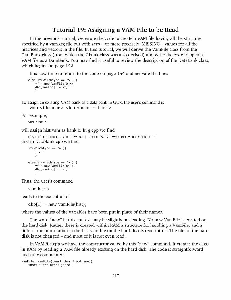
Tutorial 19: Assigning a VAM File to be ReadIn the previous tutorial, we wrote the code to create a VAM file having all the structure
specified by a vam.cfg file but with zero – or more precisely, MISSING – values for all the matrices and vectors in the file. In this tutorial, we will derive the VamFile class from the DataBank class (from which the Gbank class was also derived) and write the code to open a VAM file as a DataBank. You may find it useful to review the description of the DataBank class,which begins on page 142.
It is now time to return to the code on page 154 and activate the lines else if(whichtype == 'v') {
vf = new VamFile(bnk); dbp[bankno] = vf; }
To assign an existing VAM bank as a data bank in Gwx, the user's command isvam <filename> <letter name of bank>
For example,vam hist b
will assign hist.vam as bank b. In g.cpp we findelse if (strcmp(s,"vam") == 0 || strcmp(s,"v")==0) err = bankcmd('v');
and in DataBank.cpp we find if(whichtype == 'w'){
. . .}
else if(whichtype == 'v') { vf = new VamFile(bnk); dbp[bankno] = vf; }
Thus, the user's command
vam hist b
leads to the execution of
dbp[1] = new VamFile(hist);
where the values of the variables have been put in place of their names.
The word “new” in this context may be slightly misleading. No new VamFile is created on the hard disk. Rather there is created within RAM a structure for handling a VamFile, and a little of the information in the hist.vam file on the hard disk is read into it. The file on the harddisk is not changed – and most of it is not even read.
In VAMFile.cpp we have the constructor called by this “new” command. It creates the classin RAM by reading a VAM file already existing on the hard disk. The code is straightforward and fully commented.VamFile::VamFile(const char *rootname){
short i,err,nvecs,jahra;
217

string rn = rootname; rn += ".vam";
// rn is now rootname.vam// pbank is declared in the DataBank class from which VamFile is derived.
if((pbank=fopen(rn.c_str(),"r+b"))==NULL ){printg("Could not open %s\n",rn.c_str());return;
}// The DataBank class has a bnktitle variable but with no
// space allocated. The next two lines grab space for the // title and give the file a default blank title. bnktitle = new char[81]; strcpy(bnktitle," ");
//Read and display the VAmRile description = sizeof(struct VamFileDesc); seek(pbank, 0, SEEK_SET);
read(&fd,i,1,pbank); // should be 102 bytes
// Because of problems with reading and writing the struct,// its contents are displayed in detail.printg("File description of %s.\n",rn.c_str());
printg("Startdate %10.1f Enddate %10.1f\n",fd.startdate,fd.enddate); printg("Number of numbers per year %d, Start position %d\n", fd.numnumpy,fd.startpsn); printg("Number of vectors %d, Number of characters in vector names %d\n", fd.nvectors,fd.ncivnames);
nvecs=fd.nvectors;
// Allocate space for and read vindxvindx=new unsigned short[nvecs+1];fread(vindx,sizeof(unsigned short),nvecs+1,pbank);
// Allocate space for sizes and csizessizes=new unsigned int[nvecs];fread(sizes,sizeof(int),nvecs,pbank);
// Same for rowsrows=new unsigned short[nvecs];fread(rows,sizeof(unsigned short),nvecs,pbank);
// and for columnscolumns=new unsigned short[nvecs];fread(columns,sizeof(unsigned short),nvecs,pbank);
// and lagslags=new short[nvecs];fread(lags, sizeof(short),nvecs,pbank);
// and typestypes=new char[nvecs];fread(types,sizeof(char),nvecs,pbank);
// and finally vnamesvnames=new char[vindx[nvecs]];fread(vnames,1,vindx[nvecs],pbank);
// the stubs require a double allocation.rowstub = new char*[nvecs];colstub = new char*[nvecs];for(i=0;i<nvecs;i++){
rowstub[i]=new char[30]; fread(rowstub[i],1,30,pbank); }for(i=0;i<nvecs;i++){ colstub[i]=new char[30]; fread(colstub[i],1,30,pbank); }
218
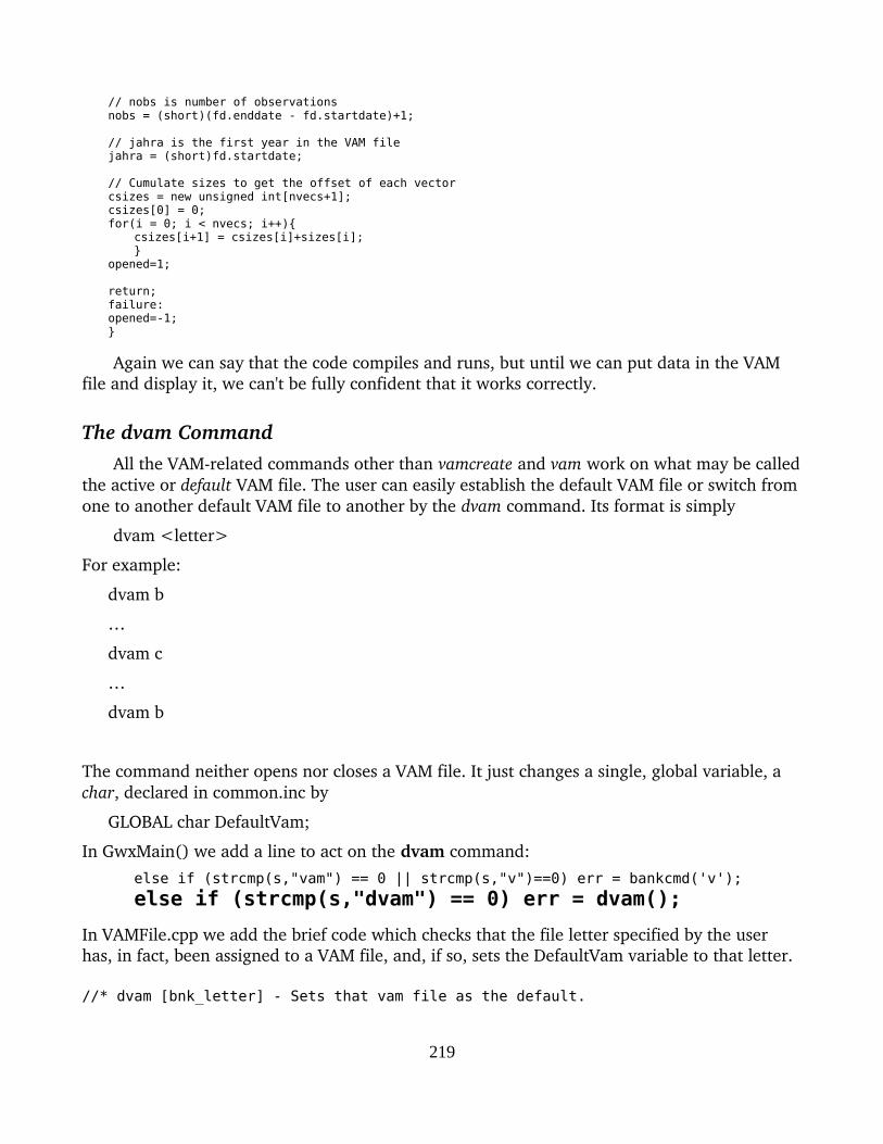
// nobs is number of observationsnobs = (short)(fd.enddate - fd.startdate)+1;
// jahra is the first year in the VAM filejahra = (short)fd.startdate;
// Cumulate sizes to get the offset of each vector csizes = new unsigned int[nvecs+1];
csizes[0] = 0;for(i = 0; i < nvecs; i++){
csizes[i+1] = csizes[i]+sizes[i];}
opened=1;
return; failure: opened=-1; }
Again we can say that the code compiles and runs, but until we can put data in the VAM file and display it, we can't be fully confident that it works correctly.
The dvam CommandAll the VAMrelated commands other than vamcreate and vam work on what may be called
the active or default VAM file. The user can easily establish the default VAM file or switch fromone to another default VAM file to another by the dvam command. Its format is simply
dvam <letter>
For example:
dvam b
…
dvam c
…
dvam b
The command neither opens nor closes a VAM file. It just changes a single, global variable, a char, declared in common.inc by
GLOBAL char DefaultVam;
In GwxMain() we add a line to act on the dvam command:
else if (strcmp(s,"vam") == 0 || strcmp(s,"v")==0) err = bankcmd('v');
else if (strcmp(s,"dvam") == 0) err = dvam();
In VAMFile.cpp we add the brief code which checks that the file letter specified by the user has, in fact, been assigned to a VAM file, and, if so, sets the DefaultVam variable to that letter.
//* dvam [bnk_letter] - Sets that vam file as the default.
219
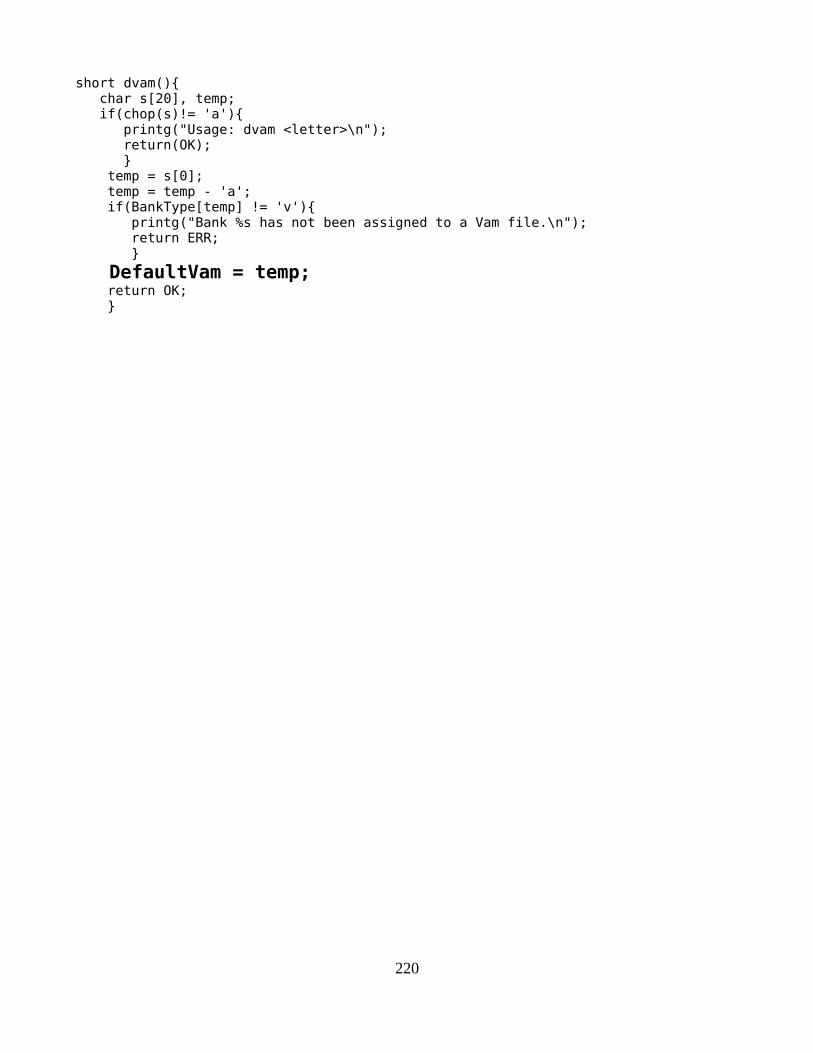
short dvam(){char s[20], temp;if(chop(s)!= 'a'){
printg("Usage: dvam <letter>\n");return(OK);}
temp = s[0]; temp = temp - 'a'; if(BankType[temp] != 'v'){
printg("Bank %s has not been assigned to a Vam file.\n"); return ERR; }
DefaultVam = temp; return OK; }
220
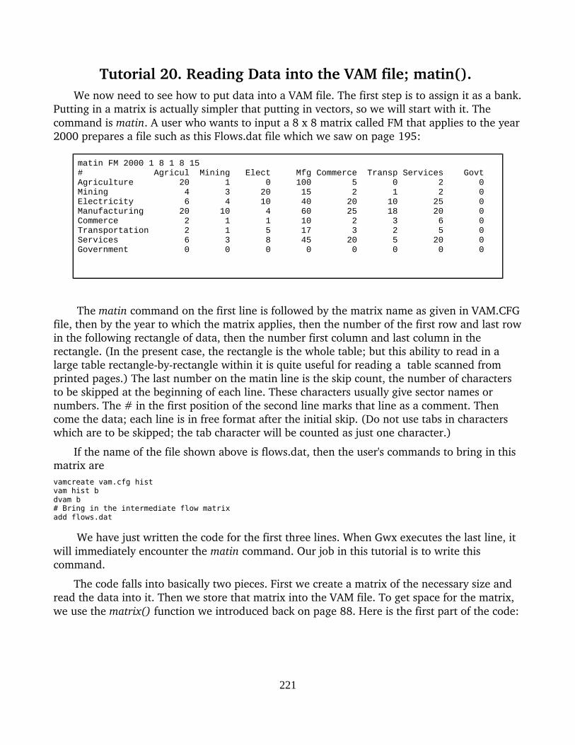
Tutorial 20. Reading Data into the VAM file; matin(). We now need to see how to put data into a VAM file. The first step is to assign it as a bank.
Putting in a matrix is actually simpler that putting in vectors, so we will start with it. The command is matin. A user who wants to input a 8 x 8 matrix called FM that applies to the year2000 prepares a file such as this Flows.dat file which we saw on page 195:
matin FM 2000 1 8 1 8 15 # Agricul Mining Elect Mfg Commerce Transp Services GovtAgriculture 20 1 0 100 5 0 2 0Mining 4 3 20 15 2 1 2 0Electricity 6 4 10 40 20 10 25 0Manufacturing 20 10 4 60 25 18 20 0Commerce 2 1 1 10 2 3 6 0Transportation 2 1 5 17 3 2 5 0Services 6 3 8 45 20 5 20 0Government 0 0 0 0 0 0 0 0
The matin command on the first line is followed by the matrix name as given in VAM.CFGfile, then by the year to which the matrix applies, then the number of the first row and last rowin the following rectangle of data, then the number first column and last column in the rectangle. (In the present case, the rectangle is the whole table; but this ability to read in a large table rectanglebyrectangle within it is quite useful for reading a table scanned from printed pages.) The last number on the matin line is the skip count, the number of characters to be skipped at the beginning of each line. These characters usually give sector names or numbers. The # in the first position of the second line marks that line as a comment. Then come the data; each line is in free format after the initial skip. (Do not use tabs in characters which are to be skipped; the tab character will be counted as just one character.)
If the name of the file shown above is flows.dat, then the user's commands to bring in this matrix arevamcreate vam.cfg histvam hist bdvam b# Bring in the intermediate flow matrixadd flows.dat
We have just written the code for the first three lines. When Gwx executes the last line, it will immediately encounter the matin command. Our job in this tutorial is to write this command.
The code falls into basically two pieces. First we create a matrix of the necessary size and read the data into it. Then we store that matrix into the VAM file. To get space for the matrix, we use the matrix() function we introduced back on page 88. Here is the first part of the code:
221
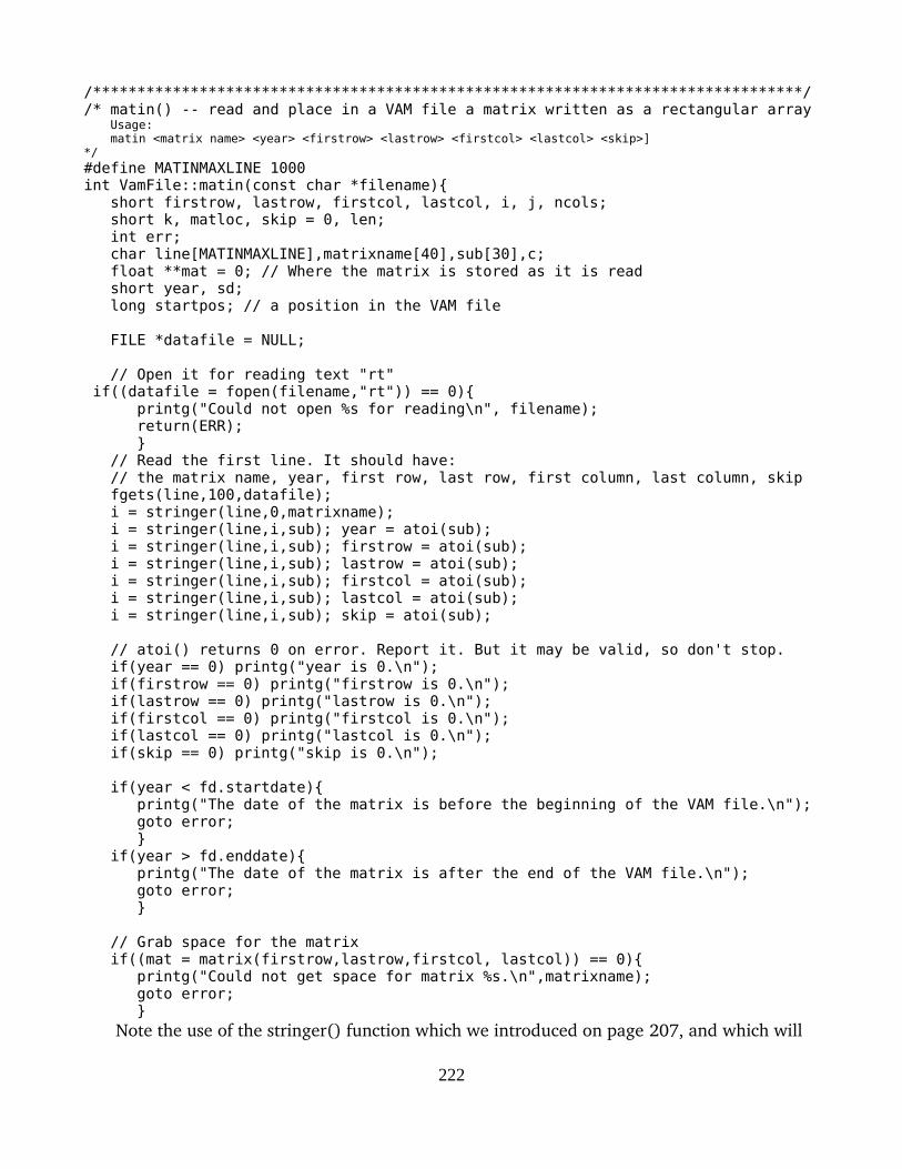
/********************************************************************************//* matin() -- read and place in a VAM file a matrix written as a rectangular array
Usage:matin <matrix name> <year> <firstrow> <lastrow> <firstcol> <lastcol> <skip>]
*/#define MATINMAXLINE 1000int VamFile::matin(const char *filename){
short firstrow, lastrow, firstcol, lastcol, i, j, ncols;short k, matloc, skip = 0, len;int err;char line[MATINMAXLINE],matrixname[40],sub[30],c;float **mat = 0; // Where the matrix is stored as it is readshort year, sd;
long startpos; // a position in the VAM file
FILE *datafile = NULL;
// Open it for reading text "rt" if((datafile = fopen(filename,"rt")) == 0){
printg("Could not open %s for reading\n", filename);return(ERR);}
// Read the first line. It should have:// the matrix name, year, first row, last row, first column, last column, skipfgets(line,100,datafile);i = stringer(line,0,matrixname);i = stringer(line,i,sub); year = atoi(sub);i = stringer(line,i,sub); firstrow = atoi(sub);i = stringer(line,i,sub); lastrow = atoi(sub);i = stringer(line,i,sub); firstcol = atoi(sub);i = stringer(line,i,sub); lastcol = atoi(sub);i = stringer(line,i,sub); skip = atoi(sub);
// atoi() returns 0 on error. Report it. But it may be valid, so don't stop.if(year == 0) printg("year is 0.\n");if(firstrow == 0) printg("firstrow is 0.\n");if(lastrow == 0) printg("lastrow is 0.\n");if(firstcol == 0) printg("firstcol is 0.\n");if(lastcol == 0) printg("lastcol is 0.\n");if(skip == 0) printg("skip is 0.\n");
if(year < fd.startdate){ printg("The date of the matrix is before the beginning of the VAM file.\n"); goto error;
}if(year > fd.enddate){
printg("The date of the matrix is after the end of the VAM file.\n"); goto error;
}
// Grab space for the matrixif((mat = matrix(firstrow,lastrow,firstcol, lastcol)) == 0){
printg("Could not get space for matrix %s.\n",matrixname); goto error;
}Note the use of the stringer() function which we introduced on page 207, and which will
222

now prove very useful in reading numbers.
// Now read and store one line at a time.
// ncols refers to the array that is read,// not to matrix in the VAM file.
ncols = lastcol - firstcol + 1;
for(i = firstrow; i <= lastrow; i++){// Read a row of the matrix into "line".readline:if(fgets(line,MATINMAXLINE-1,iin) == NULL){
printg("Unable to read row %d of matrix %s.\n",i,matrixname); goto error;
}if(line[0] == '#') goto readline; // a comment linelen = strlen(line);if(len <= skip) goto readline; //short line,nothing past the skipped area.k = skip;
// Bite off the numbers one by one, convert to floats, and store away.for(j = firstcol; j <= lastcol; j++){
k = stringer(line,k,sub);mat[i][j] = atof(sub);}
}
Note how easily the skip was accomplished with stringer().
// The matrix is now in mat. It's time to store it in the VAM file.
if((matloc = findname(matrixname)) == ERR){printg("Could not find %s in the VAM file.\n",matrixname);
goto error;}
sd = fd.startdate;for(i = firstrow; i <= lastrow; i++){
// Compute the starting position of these numbers in the VAM file.startpos = fd.startpsn + // bytes in header of VAM file
fd.numnumpy*(year -sd)*4 + // bytes is prior years' datacsizes[matloc]*4 + // bytes in prior matrices this year(i-1)*(long)columns[matloc]*4 + // bytes in prior rows this year(firstcol -1)*4; // bytes in prior columns of this row.
// Position the VAM file to that point.err = fseek(pbank, startpos, 0);// Write the row of the matrix into the VAM file.if((err = fwrite(&mat[i][firstcol],4,ncols,pbank)) != ncols){
printg("Failure trying to write row %d of matrix %s in year %d\n",i, matrixname, year);
goto error;}
}
// Success. Close up normally.if(mat) free_matrix(mat,firstrow,lastrow,firstcol);printg("Matrix %s successfully read.\n",matrixname);
223

return(OK);
error:if(mat) free_matrix(mat,firstrow,lastrow,firstcol);
return(ERR);}
/*******************************************************************/
Now we must provide a way for the user to call matin(). Since it is a member function of the VamFile class, it cannot be called in quite the same way as other functions have been called. Rather it must be called thus:
vf>matin();
so in the gselect() routine in GwxMain.cpp we find else if (strncmp(s,"vamcreate",max(len,5))== 0) err = vamcreate(); else if (strcmp(s,"dvam") == 0) err = dvam();
else if (strcmp(s,"matin") == 0) err = vf->matin();
We will write more functions which are members of the VamFile class, and they will be called in this way.
We also need to deal with getting vectors into the VamFile, but first let's see if we can display the matrix with a grid.
224
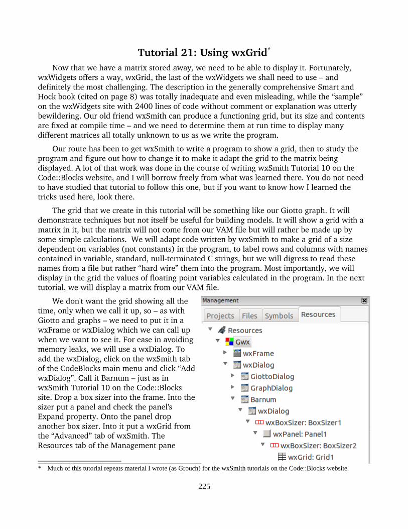
Tutorial 21: Using wxGrid*
Now that we have a matrix stored away, we need to be able to display it. Fortunately, wxWidgets offers a way, wxGrid, the last of the wxWidgets we shall need to use – and definitely the most challenging. The description in the generally comprehensive Smart and Hock book (cited on page 8) was totally inadequate and even misleading, while the “sample” on the wxWidgets site with 2400 lines of code without comment or explanation was utterly bewildering. Our old friend wxSmith can produce a functioning grid, but its size and contents are fixed at compile time – and we need to determine them at run time to display many different matrices all totally unknown to us as we write the program.
Our route has been to get wxSmith to write a program to show a grid, then to study the program and figure out how to change it to make it adapt the grid to the matrix being displayed. A lot of that work was done in the course of writing wxSmith Tutorial 10 on the Code::Blocks website, and I will borrow freely from what was learned there. You do not need to have studied that tutorial to follow this one, but if you want to know how I learned the tricks used here, look there.
The grid that we create in this tutorial will be something like our Giotto graph. It will demonstrate techniques but not itself be useful for building models. It will show a grid with a matrix in it, but the matrix will not come from our VAM file but will rather be made up by some simple calculations. We will adapt code written by wxSmith to make a grid of a size dependent on variables (not constants) in the program, to label rows and columns with names contained in variable, standard, nullterminated C strings, but we will digress to read these names from a file but rather “hard wire” them into the program. Most importantly, we will display in the grid the values of floating point variables calculated in the program. In the next tutorial, we will display a matrix from our VAM file.
We don't want the grid showing all thetime, only when we call it up, so – as withGiotto and graphs – we need to put it in awxFrame or wxDialog which we can call upwhen we want to see it. For ease in avoidingmemory leaks, we will use a wxDialog. Toadd the wxDialog, click on the wxSmith tabof the CodeBlocks main menu and click “AddwxDialog”. Call it Barnum – just as inwxSmith Tutorial 10 on the Code::Blockssite. Drop a box sizer into the frame. Into thesizer put a panel and check the panel'sExpand property. Onto the panel dropanother box sizer. Into it put a wxGrid fromthe “Advanced” tab of wxSmith. TheResources tab of the Management pane
* Much of this tutorial repeats material I wrote (as Grouch) for the wxSmith tutorials on the Code::Blocks website.
225

should now look as shown on the right.
Click on the wxGrid and in its properties window (in the lower left corner of the screen) set its number of columns to 40 and number of rows to 40; uncheck the Default size box and set the width to 400 and height to 300. (These numbers are in pixels. It is very important to unckeck that Default size box.) Click on the + inside a □ next to the word Style to drop down a listof Style features; check the box for wxFullRepaintOnResize. Finally, check the Expand box. At this point you should see encouraging signs on the right; a grid has appeared.
If you click the “Show preview” button over on the right (just under the big red X) a grid appears and you can scroll around in it. It is pretty small, but if you try to stretch it with the mouse, you will find that it won't stretch. We have forgotten something. Click on that wxDialog just under Barnum in the Resources pane. Click on the + in the square next to “Style” in its properties window. Scroll down until you get to wxRESIZE-BORDER and check it. Now when you click on “Show preview” the grid should stretch.
Do not be tempted to call for scrollbars on any of these elements. wxGrid automatically provides scrollbars and calling for others seems just to confuse matters.
The Barnum codeWe find the code that wxSmith has written for us in Barnum.cpp. There we see that this
code falls into three parts: (1) an introduction which we do not need to change, (2) a substantive middle portion which we must change, and (3) a generic conclusion we do not need to change. Below is what we find in the present case, where I have marked the parts and have already written a middle part to display in the grid a numerical matrix with some of the rows and columns labeled.
The crucial thing to note here is that only a wxString can go into a cell of the grid or into a row or column label. We will use one and only one wxString variable, carpet. Everything we want to show in the grid we first put on carpet, and on carpet it then flies into the grid. The tricky part is how to convert floats and standard, nullterminated C strings into wxStrings. I found the answers on the Internet and use those methods here. The lines that do this conversion are in bold; everything else in Part 2 is pretty simple.
226
Sometimes you may want to get rid of a wxDialog or other “resource” you added to the project by means of the wxSmith tab. The big red X on the right which removes other things will not remove the wxDialog. Rather you must right click on the name of the wxDialog in the management pane and select “Delete this resource.” There is no undoing this action. I had a misbehaving wxDialog that had to be totally removed and learned about the right click by trying everything.
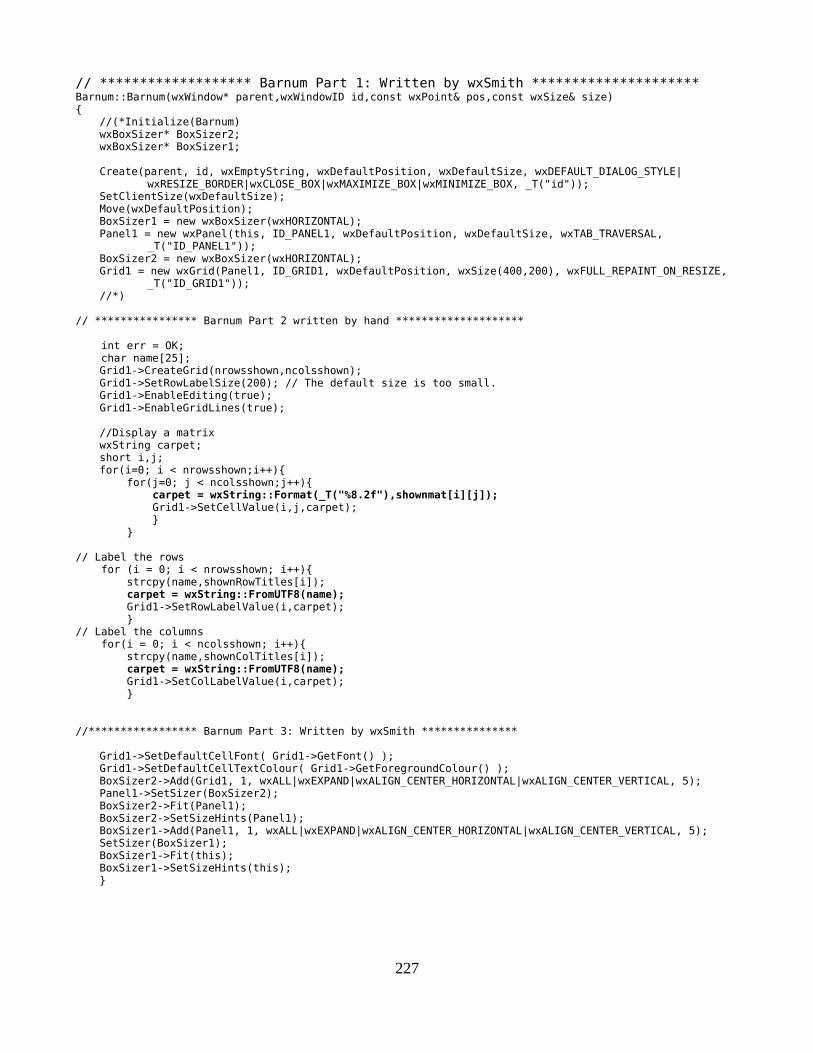
// ******************* Barnum Part 1: Written by wxSmith *********************Barnum::Barnum(wxWindow* parent,wxWindowID id,const wxPoint& pos,const wxSize& size) {
//(*Initialize(Barnum) wxBoxSizer* BoxSizer2; wxBoxSizer* BoxSizer1;
Create(parent, id, wxEmptyString, wxDefaultPosition, wxDefaultSize, wxDEFAULT_DIALOG_STYLE|wxRESIZE_BORDER|wxCLOSE_BOX|wxMAXIMIZE_BOX|wxMINIMIZE_BOX, _T("id"));
SetClientSize(wxDefaultSize); Move(wxDefaultPosition); BoxSizer1 = new wxBoxSizer(wxHORIZONTAL); Panel1 = new wxPanel(this, ID_PANEL1, wxDefaultPosition, wxDefaultSize, wxTAB_TRAVERSAL,
_T("ID_PANEL1")); BoxSizer2 = new wxBoxSizer(wxHORIZONTAL); Grid1 = new wxGrid(Panel1, ID_GRID1, wxDefaultPosition, wxSize(400,200), wxFULL_REPAINT_ON_RESIZE,
_T("ID_GRID1")); //*)
// **************** Barnum Part 2 written by hand ********************
int err = OK; char name[25];
Grid1->CreateGrid(nrowsshown,ncolsshown); Grid1->SetRowLabelSize(200); // The default size is too small.Grid1->EnableEditing(true); Grid1->EnableGridLines(true);
//Display a matrix wxString carpet; short i,j; for(i=0; i < nrowsshown;i++){
for(j=0; j < ncolsshown;j++){ carpet = wxString::Format(_T("%8.2f"),shownmat[i][j]); Grid1->SetCellValue(i,j,carpet); } }
// Label the rows for (i = 0; i < nrowsshown; i++){ strcpy(name,shownRowTitles[i]); carpet = wxString::FromUTF8(name); Grid1->SetRowLabelValue(i,carpet); } // Label the columns for(i = 0; i < ncolsshown; i++){ strcpy(name,shownColTitles[i]); carpet = wxString::FromUTF8(name); Grid1->SetColLabelValue(i,carpet); }
//***************** Barnum Part 3: Written by wxSmith ***************
Grid1->SetDefaultCellFont( Grid1->GetFont() ); Grid1->SetDefaultCellTextColour( Grid1->GetForegroundColour() ); BoxSizer2->Add(Grid1, 1, wxALL|wxEXPAND|wxALIGN_CENTER_HORIZONTAL|wxALIGN_CENTER_VERTICAL, 5); Panel1->SetSizer(BoxSizer2); BoxSizer2->Fit(Panel1); BoxSizer2->SetSizeHints(Panel1); BoxSizer1->Add(Panel1, 1, wxALL|wxEXPAND|wxALIGN_CENTER_HORIZONTAL|wxALIGN_CENTER_VERTICAL, 5); SetSizer(BoxSizer1); BoxSizer1->Fit(this); BoxSizer1->SetSizeHints(this); }
227

Barnum::~Barnum() {
//(*Destroy(Barnum) //*)
}
Preparing the matrix to be shown: showmat():We now need to prepare shownmat, the matrix to be displayed, and a way for the user to call for its
preparation and display. Down near the bottom of the long list of “else if” commands in GwxMain.cpp,stick in the show() command:
else if (strncmp(s,"bank",max(len,2))== 0 || strcmp(s,"b")==0) err = bankcmd('w'); else if (strcmp(s,"show") == 0) err = showmat(); else if(strncmp(s,"quit",std::max(len,1)) == 0) exit(0);
In writing showmat(), I have made a gesture toward the next tutorial. The behavior that I want in the end is that if the user types just “show”, he will get our demo; but if he types something like “show FM y 2000” he will get a matrix read from the default VAM file. In this tutorial, we will just have the program detect whether there is anything after the word “show”.If not, our demo will appear somewhat reminiscent of old Giotto; but if so, we just get a reminder that presently only the demo works. This switching is accomplished by a Boolean variable – demo – which is true if the demo is to be shown. But really reading a matrix is left tothe next tutorial.
First we add some new global variables to the common.h file:GLOBAL char DefaultVam;GLOBAL float **shownmat; // pointer for matrix to be shown.GLOBAL short nrowsshown, ncolsshown;// number of rows and cols of shown matrix.GLOBAL char shownRowTitles[10][25];GLOBAL char shownColTitles[10][12];
When we add the reading of titles from a file, we will have to return to the question of making space for them, but for the moment the fixed amount of space will do. We will initiallyjust tack the showmat() function onto the end of the functions.cpp file, so in common.h we need to add showmat() like this:
short atoq(float *f);short atoqi(float *f);
short showmat();
and at the end of functions.cpp we put:
short showmat(){ bool demo; demo = false; short i,j,year; float xij; char name[40]; // Name of the matrix to be shown. char *pnam,vnam[32],type[8];
// Simulate reading a file of titles with these fixed titles. strcpy(shownRowTitles[0],"1 Agriculture"); strcpy(shownRowTitles[1],"2 Mining"); strcpy(shownRowTitles[2],"3 Utilities"); strcpy(shownRowTitles[3],"4 Manufacturing"); strcpy(shownRowTitles[4],"5 Commerce");
228

strcpy(shownRowTitles[5],"6 Transportation"); strcpy(shownRowTitles[6],"7 Services"); strcpy(shownRowTitles[7],"8 Government");
strcpy(shownColTitles[0],"1 Agric"); strcpy(shownColTitles[1],"2 Mining"); strcpy(shownColTitles[2],"3 Util"); strcpy(shownColTitles[3],"4 Mfg"); strcpy(shownColTitles[4],"5 Comm"); strcpy(shownColTitles[5],"6 Trans"); strcpy(shownColTitles[6],"7 Serv"); strcpy(shownColTitles[7],"8 Govt");
// If no name is given, show the demo. if((chop(name)) != 'a') demo = true; if(demo){ nrowsshown = 20; ncolsshown = 30; shownmat = matrix(0,nrowsshown,0,ncolsshown); for (i = 0; i < nrowsshown;i++){ for(j=0; j < ncolsshown; j++){ xij = i+j; shownmat[i][j] = xij/2.0; } }
Barnum *pt = new Barnum(NULL); pt->ShowModal(); delete pt; free_matrix(shownmat,0,nrowsshown,0); } else {
printg(“Not yet ready for more than the demo.\n”); } return OK; }
The choice of pt as the name of the created instance of Barnum is arbitrary; the letters are just old Barnum's initials. Everything else has to be just as it is. Because we have used “ShowModal”, the program does not get to the “delete” line until the user has closed the dialogwith the grid. But because we then promptly “delete” the instance of Barnum – that is to say, we release the space in memory which the “new” command grabbed for it – we should not experience any memory leak.
There is one more thing that must be done before the program will compile. wxSmith created a header file to go with Barnum but it did not “include” it in the program. We must do so. Run the scrollbar up to the top of functions.cpp. You should see:
#include "common.h"
Below it add:
#include "Barnum.h"
Compile, run, and give the command show. With a little bit of luck, you will see this:
229

The scrollbars, the orange lines at bottom left and top right, should work. Or you can click in the grid and run around with the arrow keys.
The close student of the wxSmith tutorial on the Code::Blocks website may have noticed that there the code executed when the button was clicked to bring up the grid was:
Barnum *pt = new Barnum(this); pt->ShowModal(); delete pt;
whereas here we have Barnum *pt = new Barnum(NULL); pt->ShowModal(); delete pt;
The difference is in the argument to Barnum; there this, here NULL. With this in place of NULL in the call from showmat(), the program simply won't compile. This is exactly the same problem we encountered with graphs back on page 131. What works with a button does not work with an ordinary call. Just why this is so eludes me, but the substitution of NULL in placeof this seems to work fine.
It is possible to widen the row labels and to heighten the column labels in wxSmith, but I have found no way to get two lines into the column labels nor to have one or more fixed rows (other than the labels) that do not disappear as one scrolls down.
230
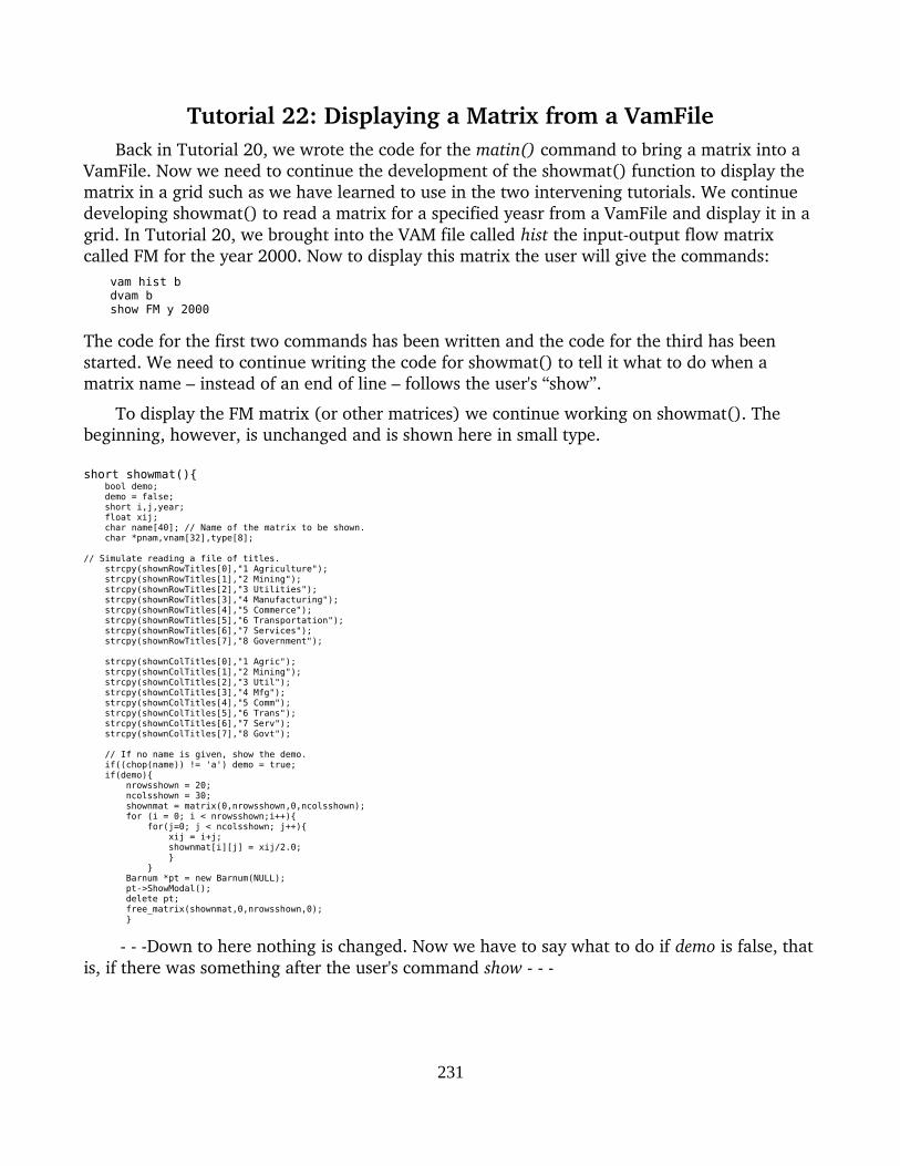
Tutorial 22: Displaying a Matrix from a VamFileBack in Tutorial 20, we wrote the code for the matin() command to bring a matrix into a
VamFile. Now we need to continue the development of the showmat() function to display the matrix in a grid such as we have learned to use in the two intervening tutorials. We continue developing showmat() to read a matrix for a specified yeasr from a VamFile and display it in a grid. In Tutorial 20, we brought into the VAM file called hist the inputoutput flow matrix called FM for the year 2000. Now to display this matrix the user will give the commands:
vam hist bdvam bshow FM y 2000
The code for the first two commands has been written and the code for the third has been started. We need to continue writing the code for showmat() to tell it what to do when a matrix name – instead of an end of line – follows the user's “show”.
To display the FM matrix (or other matrices) we continue working on showmat(). The beginning, however, is unchanged and is shown here in small type.
short showmat(){ bool demo; demo = false; short i,j,year; float xij; char name[40]; // Name of the matrix to be shown. char *pnam,vnam[32],type[8];
// Simulate reading a file of titles. strcpy(shownRowTitles[0],"1 Agriculture"); strcpy(shownRowTitles[1],"2 Mining"); strcpy(shownRowTitles[2],"3 Utilities"); strcpy(shownRowTitles[3],"4 Manufacturing"); strcpy(shownRowTitles[4],"5 Commerce"); strcpy(shownRowTitles[5],"6 Transportation"); strcpy(shownRowTitles[6],"7 Services"); strcpy(shownRowTitles[7],"8 Government");
strcpy(shownColTitles[0],"1 Agric"); strcpy(shownColTitles[1],"2 Mining"); strcpy(shownColTitles[2],"3 Util"); strcpy(shownColTitles[3],"4 Mfg"); strcpy(shownColTitles[4],"5 Comm"); strcpy(shownColTitles[5],"6 Trans"); strcpy(shownColTitles[6],"7 Serv"); strcpy(shownColTitles[7],"8 Govt");
// If no name is given, show the demo. if((chop(name)) != 'a') demo = true; if(demo){ nrowsshown = 20; ncolsshown = 30; shownmat = matrix(0,nrowsshown,0,ncolsshown); for (i = 0; i < nrowsshown;i++){ for(j=0; j < ncolsshown; j++){ xij = i+j; shownmat[i][j] = xij/2.0; } } Barnum *pt = new Barnum(NULL); pt->ShowModal(); delete pt; free_matrix(shownmat,0,nrowsshown,0); }
Down to here nothing is changed. Now we have to say what to do if demo is false, thatis, if there was something after the user's command show
231
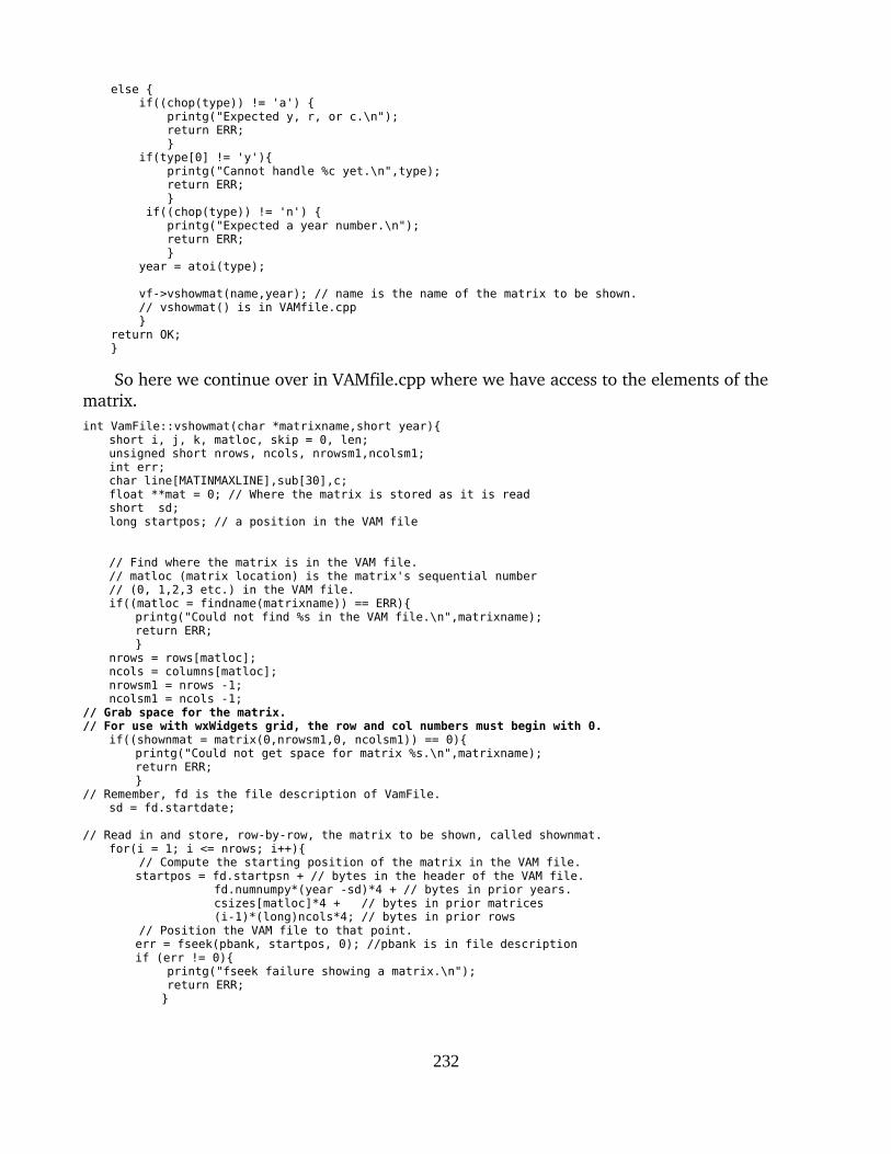
else { if((chop(type)) != 'a') { printg("Expected y, r, or c.\n"); return ERR; } if(type[0] != 'y'){ printg("Cannot handle %c yet.\n",type); return ERR; } if((chop(type)) != 'n') { printg("Expected a year number.\n"); return ERR; } year = atoi(type);
vf->vshowmat(name,year); // name is the name of the matrix to be shown. // vshowmat() is in VAMfile.cpp } return OK; }
So here we continue over in VAMfile.cpp where we have access to the elements of the matrix.int VamFile::vshowmat(char *matrixname,short year){
short i, j, k, matloc, skip = 0, len;unsigned short nrows, ncols, nrowsm1,ncolsm1;int err;char line[MATINMAXLINE],sub[30],c;float **mat = 0; // Where the matrix is stored as it is readshort sd;
long startpos; // a position in the VAM file
// Find where the matrix is in the VAM file.// matloc (matrix location) is the matrix's sequential number// (0, 1,2,3 etc.) in the VAM file.if((matloc = findname(matrixname)) == ERR){
printg("Could not find %s in the VAM file.\n",matrixname); return ERR;
}nrows = rows[matloc];ncols = columns[matloc];nrowsm1 = nrows -1;ncolsm1 = ncols -1;
// Grab space for the matrix. // For use with wxWidgets grid, the row and col numbers must begin with 0.
if((shownmat = matrix(0,nrowsm1,0, ncolsm1)) == 0){printg("Could not get space for matrix %s.\n",matrixname);
return ERR;}
// Remember, fd is the file description of VamFile.sd = fd.startdate;
// Read in and store, row-by-row, the matrix to be shown, called shownmat.for(i = 1; i <= nrows; i++){
// Compute the starting position of the matrix in the VAM file.startpos = fd.startpsn + // bytes in the header of the VAM file.
fd.numnumpy*(year -sd)*4 + // bytes in prior years.csizes[matloc]*4 + // bytes in prior matrices(i-1)*(long)ncols*4; // bytes in prior rows
// Position the VAM file to that point.err = fseek(pbank, startpos, 0); //pbank is in file descriptionif (err != 0){
printg("fseek failure showing a matrix.\n"); return ERR;
}
232

// Read the row of the matrix from the VAM file into mat.if((err = fread(&shownmat[i-1][0],4,ncols,pbank)) != ncols){
printg("Failure trying to read row %d of matrix %s in year %d\n",i, matrixname, year); return ERR;
} } nrowsshown = nrows; ncolsshown = ncols;
// Show the matrix without a grid for checking.// Remove when confident that the grid is working right. for (i = 0; i < nrows; i++){ for(j =0; j < ncols;j++){ printg("%8.0f ", shownmat[i][j]); } printg("\n"); }// shownmat is now ready for Barnum
Barnum *pt = new Barnum(NULL); pt->ShowModal(); delete pt;
free_matrix(shownmat,0,nrowsm1,0);
return OK;}
Compile, run, and give Gwx the commands
vam hist b
dvam b
show FM y 2000
and you can hope to see, as I did, the following display of the inputoutput flow matrix we introduced with the matin command back in Tutorial 20.
233

This is the end for the May 2017 edition of The Gwx Story. I hope to continue somewhat farther. In particular, reading of row and column titles for a matrix must be added to make thematrix display capability truly useful.
At the end of Tutorial 17, we listed 17 capabilities we needed to add to Gwx. We have now added the first 7, including the most challenging one, the show() command with its use ofwxGrid. It would be premature to say that the end is in sight, but with wxGrid working we cansafely say that what we set out to do – rewrite G7 with opensource, crossplatform tools, and explain each step – is doable.
234