the government budget: some facts and figures chapter...

1

© 2008 Pearson Addison-Wesley. All rights reserved

Chapter 15

Government Spending and its Financing

© 2008 Pearson Addison-Wesley. All rights reserved 15-2

Chapter Outline

• The Government Budget: Some Facts and Figures• Government Spending, Taxes, and the Macroeconomy• Government Deficits and Debt• Deficits and Inflation


The Government Budget: Some Facts and Figures

• Government outlays; three categories of government expenditures– Government purchases (G)– Transfer payments (TR)– Net interest payments (INT)

– Also: Subsidies less surpluses of government enterprises; relatively small, so we ignore it


• Government outlays; three categories of government expenditures– Government purchases (G)

• Government investment, which is about 1/6 of total government purchases, consists of purchases of capital goods

• Government consumption expenditures are about 5/6 of total government purchases


2


• Government outlays; three categories of government expenditures– Transfer payments (TR)

• Transfers are expenditures for which the government receives no current goods or services in return

• Examples: social security benefits, pensions for government retirees, welfare payments



• Government outlays; three categories of government expenditures– Net interest payments (INT)

• Interest paid to holders of government bonds less interest received by the government

• Government makes loans to students, farmers, small businesses



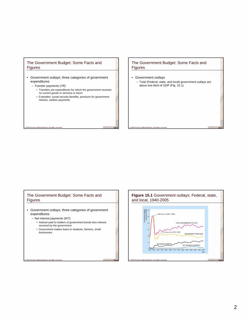
• Government outlays– Total (Federal, state, and local) government outlays are

about one-third of GDP (Fig. 15.1)



Figure 15.1 Government outlays: Federal, state, and local, 1940-2005

3


• Government outlays– Government purchases increased enormously in

World War II• Government purchases rose in other wars as well• Since the late 1960s, government purchases have drifted

downward from about 23% of GDP to about 19% of GDP



• Government outlays– Transfer payments have been rising steadily

• They’re now about 12% of GDP• Many social programs, including Social Security, Medicare, and

Medicaid, have expanded over time



• Government outlays– Net interest payments have also changed over time

• They doubled between 1941 and 1946 because of the higher debt to finance World War II

• They nearly doubled in the 1980s, as both the government debt and interest rates increased sharply

• They declined in the 1990s because of lower interest rates and government budget surpluses



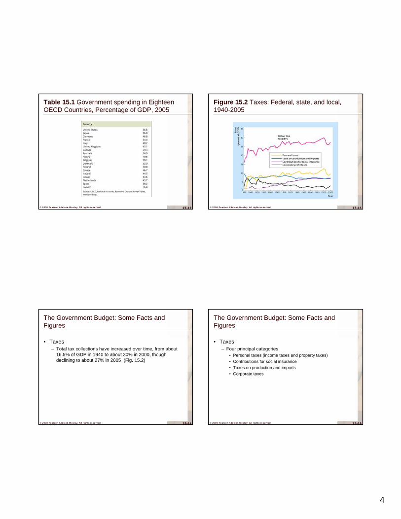
• Government outlays– Comparing U.S. government spending to that of other

countries shows that the United States spends less as a percentage of GDP than almost any other OECD country (Table 15.1)


4


Table 15.1 Government spending in Eighteen OECD Countries, Percentage of GDP, 2005


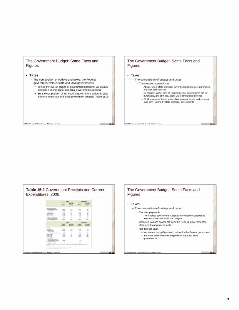
• Taxes– Total tax collections have increased over time, from about

16.5% of GDP in 1940 to about 30% in 2000, though declining to about 27% in 2005 (Fig. 15.2)



Figure 15.2 Taxes: Federal, state, and local, 1940-2005


• Taxes– Four principal categories

• Personal taxes (income taxes and property taxes)• Contributions for social insurance• Taxes on production and imports • Corporate taxes


5


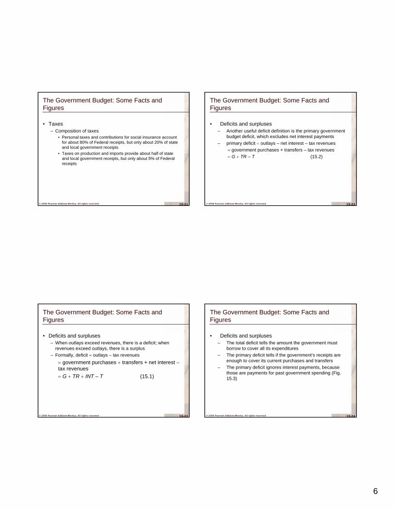
• Taxes– The composition of outlays and taxes: the Federal

government versus state and local governments• To see the overall picture of government spending, we usually

combine Federal, state, and local government spending• But the composition of the Federal government budget is quite

different from state and local government budgets (Table 15.2)



Table 15.2 Government Receipts and Current Expenditures, 2005


• Taxes– The composition of outlays and taxes

• Consumption expenditures– About 75% of state and local current expenditures are purchases

of goods and services– By contrast, about 30% of Federal current expenditures are for

purchases, and of those, about 2/3 is for national defense– Of all government purchases of nondefense goods and services,

over 80% is done by state and local governments



• Taxes– The composition of outlays and taxes:

• Transfer payments– The Federal government budget is more heavily weighted to

transfers than state and local budgets• Grants-in-aid are payments from the Federal government to

state and local governments• Net interest paid

– Net interest is significant and positive for the Federal government– It is small and sometimes negative for state and local

governments


6


• Taxes– Composition of taxes

• Personal taxes and contributions for social insurance account for about 80% of Federal receipts, but only about 20% of state and local government receipts

• Taxes on production and imports provide about half of state and local government receipts, but only about 5% of Federal receipts



• Deficits and surpluses– When outlays exceed revenues, there is a deficit; when

revenues exceed outlays, there is a surplus– Formally, deficit = outlays – tax revenues

= government purchases + transfers + net interest –tax revenues= G + TR + INT – T (15.1)



• Deficits and surpluses– Another useful deficit definition is the primary government

budget deficit, which excludes net interest payments– primary deficit = outlays – net interest – tax revenues

= government purchases + transfers – tax revenues= G + TR – T (15.2)



• Deficits and surpluses– The total deficit tells the amount the government must

borrow to cover all its expenditures– The primary deficit tells if the government’s receipts are

enough to cover its current purchases and transfers– The primary deficit ignores interest payments, because

those are payments for past government spending (Fig. 15.3)


7


Figure 15.3 The relationship between the total budget deficit and the primary deficit


• Deficits and surpluses– The separation of government purchases into government

investment and government consumption expenditures introduces another set of deficit concepts

• The current deficit equals the deficit minus government investment

• The primary current deficit equals the primary deficit minus government investment, which equals the current deficit minus interest payments



• Deficits and surpluses– The current deficit and primary current deficit usually move

together over time (Fig. 15.4)• Large current deficits occurred in World War II, the mid-

1970s, and the early 1980s• The primary current deficit became a primary surplus in some

years in the 1980s and 1990s, but large interest payments kept the overall deficit large until the late 1990s



Figure 15.4 Deficits and primary deficits: Federal, state, and local, 1940-2005

8


Government Spending, Taxes, and the Macroeconomy

• Fiscal policy and aggregate demand– An increase in government purchases increases aggregate

demand by shifting the IS curve up– The effect of tax changes depends on the economic model

• Classical economists accept the Ricardian equivalence proposition that lump-sum tax changes have no effect on national saving or on aggregate demand

• Keynesians think a tax cut is likely to increase consumption and decrease saving, thus increasing aggregate demand



• Fiscal policy and aggregate demand– Classicals and Keynesians disagree about using fiscal policy

to stabilize the economy• Classicals oppose activist policy while Keynesians favor it• But even Keynesians admit that fiscal policy is difficult to use

– There is a lack of flexibility, because much of government spending is committed years in advance

– There are long time lags, because the political process takes time to make changes



• Fiscal policy and aggregate demand– Automatic stabilizers and the full-employment deficit

• Automatic stabilizers cause fiscal policy to be countercyclical by changing government spending or taxes automatically

• One example is unemployment insurance, which causes transfers to rise in recessions

• The most important automatic stabilizer is the income tax system, since people pay less tax when their incomes are low in recessions, and they pay more tax when their incomes are high in booms



• Fiscal policy and aggregate demand– Because of automatic stabilizers, the government budget

deficit rises in recessions and falls in booms• The full-employment deficit is a measure of what the

government budget deficit would be if the economy were at full employment

• So the full-employment deficit doesn’t change with the business cycle, only with changes in government policy regarding spending and taxation

• The actual budget deficit is much larger than the full-employment budget deficit in recessions (Fig. 15.5)

9


Figure 15.5 Full-employment and actual budget deficits, 1960-2005



• Government capital formation– Fiscal policy affects the economy through the formation of

government capital—long-lived physical assets owned by the government, like roads, schools, and sewer systems

– Also, fiscal policy affects human capital formation through expenditures on health, nutrition, and education

– Data on government investment include only physical capital, nothuman capital

• In 2005, 2/3 of federal government investment was on national defense and 1/3 on nondefense capital

• Most federal government investment is in equipment, but most state and local government investment is for structures



• Incentive effects of fiscal policy– Average versus marginal tax rates

• Average tax rate = total taxes / pretax income• Marginal tax rate = taxes due from an additional dollar of

income




• Example: Suppose taxes are imposed at a rate of 25% on income over $10,000 (Table 15.3)

– For someone earning less than $10,000, the marginal tax rate and average tax rate are both zero

– Anyone earning over $10,000 would have a marginal tax rate of .25

10


Table 15.3 Marginal and average tax rates: an example (Total Tax = 25% of Income over $10,000)




• The distinction between average and marginal tax rates affects people’s decisions about how much labor to supply

– If the average tax rate increases, with the marginal tax rate held constant, a person will increase labor supply

– The higher average tax rate causes an income effect– With lower income, a person consumes less and wants less

leisure, so he or she works more– The labor supply curve shifts right




• If the marginal tax rate increases, with the average tax rate held constant, a person will decrease labor supply

– The higher marginal tax rate causes a substitution effect– With a lower after-tax reward for working, a person wants to work

less– The labor supply curve shifts left



• Tax reform proposals in 2005– The tax code distorts economic behavior– President Bush appointed a panel in 2005 to find ways to

make the tax code simpler and fairer

11



• Tax reform proposals in 2005– The panel found that

• the tax system should be streamlined and made easier• marginal tax rates should be reduced for everyone• tax benefits for homeownership and charitable donations

should go to everyone, not just those who itemize deductions• health insurance should not be taxed• the tax system should encourage saving and investment• the Alternative Minimum Tax should be repealed

– Passage of the plan faces large political hurdles



• Application: Labor supply and tax reform in the 1980s– Congress reduced tax rates twice in the 1980s

• At the beginning of the decade the highest marginal tax rate on labor income was 50%

• The 1981 tax act (ERTA) reduced tax rates in three stages, phased in until 1984

• The tax reform of 1986 further reduced personal tax rates, dropping the top marginal tax rate to 28%

– Supply-side economists promoted the tax rate reductions, arguing that labor supply, saving, and investment would all increase substantially



• Application: Labor supply and tax reform in the 1980s– Both marginal and average tax rates declined from the 1981

tax cut• The decline in the marginal tax rate should lead to increased

labor supply• The decline in the average tax rate should lead to decreased

labor supply• The overall effect is ambiguous and may be small• The data suggest little effect, as the labor force participation

rate didn’t change much after 1981



• Application: Labor supply and tax reform in the 1980s– The 1986 tax reform lowered marginal tax rates on labor

income and raised average tax rates • Both should lead to increased labor supply• The data confirm this result, as men’s labor force participation,

which had been falling over time, leveled off in 1988 and rose in 1989

– The changes in labor supply are consistent with theory, but not nearly as dramatic as projected by the supply-siders

12



• Tax-induced distortions and tax rate smoothing– In the absence of taxes, the free market works efficiently

• Taxes change economic behavior, reducing welfare• Thus tax-induced deviations from free-market outcomes are

called distortions– The difference between the number of hours a worker would

work without taxes and the number of hours he or she actually works when there is a tax reflects the tax distortion



• Tax-induced distortions and tax rate smoothing– The higher the tax rate, the greater the distortion– Fiscal policymakers would like to raise the needed amount

of government revenue while minimizing distortions



• Tax-induced distortions and tax rate smoothing– It’s better to keep the tax rate constant over time than to

raise it and lower it, because the higher tax rate has a higher distortion

• For example, keeping the tax rate at a steady 15% is better than having it at 10% one year and 20% the next, since the distortions in the second year are much higher

• Keeping a constant tax rate over time is called tax rate smoothing



• Tax-induced distortions and tax rate smoothing– Empirical studies suggest that the Federal government

hasn’t always smoothed tax rates as much as it could to minimize distortions

– But borrowing to finance wars, thus avoiding the need to raise taxes a lot in war years, is consistent with the idea of tax rate smoothing

13


Government Deficits and Debt

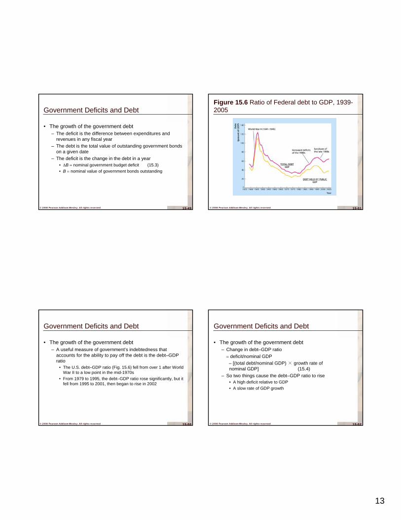
• The growth of the government debt– The deficit is the difference between expenditures and

revenues in any fiscal year– The debt is the total value of outstanding government bonds

on a given date– The deficit is the change in the debt in a year

• ΔB = nominal government budget deficit (15.3)• B = nominal value of government bonds outstanding



• The growth of the government debt– A useful measure of government’s indebtedness that

accounts for the ability to pay off the debt is the debt–GDP ratio

• The U.S. debt–GDP ratio (Fig. 15.6) fell from over 1 after World War II to a low point in the mid-1970s

• From 1979 to 1995, the debt–GDP ratio rose significantly, but it fell from 1995 to 2001, then began to rise in 2002


Figure 15.6 Ratio of Federal debt to GDP, 1939-2005



• The growth of the government debt– Change in debt–GDP ratio = deficit/nominal GDP – [(total debt/nominal GDP) × growth rate of nominal GDP] (15.4)

– So two things cause the debt–GDP ratio to rise• A high deficit relative to GDP• A slow rate of GDP growth

14



• The growth of the government debt– During World War II, large deficits raised the debt–GDP ratio– For the next 35 years, deficits were small or negative, and

GDP growth was rapid, so the debt–GDP ratio fell– During the 1980s and early 1990s, the debt–GDP ratio rose

because of high deficits– Large surpluses reduced the debt-GDP ratio in the late

1990s, but large deficits raised it beginning in 2002



• Application: Social Security: How can it be fixed?– The Social Security system may not be able to pay future

promised benefits– The system is mostly pay as you go, so that most taxes

collected today go to paying benefits to current retirees—there is only a small trust fund



• Application: Social Security: How can it be fixed?– The pay-as-you-go system worked as long as the number of

workers greatly exceeded the number of retirees, but demographic changes will soon decrease the ratio of workers to retirees

– The result will be payouts in excess of tax revenue (Fig. 15.7)


Figure 15.7 Social security cost and tax revenue as a percent of GDP, 1990-2080

15



• Application: Social Security: How can it be fixed?– Fixing the social security system

• Increase tax revenue by raising taxes, but this distorts labor supply decisions

• Increase the rate of return by investing in the stock market, but this is risky

• Reduce benefits by increasing retirement age• Allow people to invest their own funds in individual accounts

– But then there would not be enough funds to pay current retirees



• The burden of the government debt on future generations– People worry that their children will have to pay back the

debt that past generations have accumulated– But U.S. citizens own most government bonds, so future

generations will just be paying themselves



• The burden of the government debt on future generations– However, there could be a burden, because if tax rates have

to be raised in the future to pay off the debt, the higher tax rates could be distortionary

– Also, since bondholders are richer on average than nonbondholders, when the debt was repaid there would be a large transfer from the poor to the rich



• The burden of the government debt on future generations– Finally, government deficits reduce national saving

according to many economists• If so, with lower saving there will be lower investment• Lower investment means a smaller capital stock• A smaller capital stock means less output in the future• So the future standard of living will be lower• However, this assumes that government deficits reduce

national saving; that is a key and unsettled question

16



• Budget deficits and national saving: Ricardianequivalence revisited– When will a government deficit reduce national saving?

• It almost certainly does when government spending rises• But it may not for a cut in taxes or increase in transfers



• Budget deficits and national saving: Ricardianequivalence revisited– Ricardian equivalence: an example

• Suppose the government cuts taxes by $100 per person• Since S = Y – C – G, (15.5)

national saving declines only if consumption rises (assuming Y is fixed at its full-employment level)



• Budget deficits and national saving: Ricardianequivalence revisited– Consumption might not rise if people realize that a tax cut

today must be financed by higher taxes in the future• A tax cut of $100 per person could be financed by a tax

increase of (1 + r)$100 next year• Then taxpayers’ ability to consume is the same with or without

the tax cut• People will simply save the tax cut so they can pay off the

future taxes– As a result, national saving should be unaffected



• Ricardian equivalence across generations– What if the higher future taxes are to be paid by future

generations?– Then people might consume more today, because they

wouldn’t have to pay the higher future taxes

17



• Ricardian equivalence across generations– But as Barro pointed out, if people care about their children,

they’ll increase their bequests to their children so their children can pay the higher future taxes

• After all, if people wanted to consume at their children’s expense, they could have lowered their planned bequests

• So why should the fact that the government gives people a tax cut cause them to consume at their children’s expense?



• Departures from Ricardian equivalence– The data show that Ricardian equivalence holds sometimes,

but not always• It certainly didn’t hold in the United States in the 1980s, when

high government deficits were accompanied by low savings• It did seem to hold in Canada and Israel sometimes• But overall, there seems to be little relationship between

government budget deficits and national saving



• Departures from Ricardian equivalence– What are the main reasons Ricardian equivalence may fail?

• Borrowing constraints– If people can’t borrow as much as they would like, a tax cut

financed by higher future taxes essentially lets them borrow from the government

• Shortsightedness– If people don’t foresee the higher future taxes, or spend based on

rules of thumb about their current after-tax income, they may increase consumption in response to a tax cut



• Departures from Ricardian equivalence– What are the main reasons Ricardian equivalence may fail?

• Failure to leave bequests– People may not leave bequests because they don’t care about

their children, or because they think their children will be richer than they are, so they will increase consumption spending in response to a tax cut

• Non–lump-sum taxes– When taxes aren’t lump sum, changes in tax rates affect

economic decisions– However, a tax cut won’t necessarily lead to an increase in

consumption in this case

18


Deficits and Inflation

• The deficit and the money supply– Inflation results when aggregate demand rises more quickly

than aggregate supply– Budget deficits could be related to inflation, but we usually

think of expansionary fiscal policy as leading to a one-time jump in the price level, not a sustained inflation

– The only way for a sustained inflation to occur is for there to be sustained growth in the money supply



• The deficit and the money supply– Can government deficits lead to ongoing increases in the

money supply?• Yes, if spending is financed by printing money• The revenue that a government raises by printing money is

called seignorage• Usually, governments don’t just buy things directly with newly

printed money, they do so indirectly– The Treasury borrows by issuing government bonds– The central bank buys the bonds with newly printed money



• The deficit and the money supply– The relationship between the deficit and the increase in the monetary

base isdeficit = ΔB = ΔBp + ΔBcb = ΔBp + ΔBASE (15.6)

– ΔB is the increase in government debt, which is divided into government debt held by the public Bp and government debt held by the central bank Bcb

– Changes in Bcb equal changes in the monetary base, BASE– In an all-currency economy, the change in the monetary base is equal to

the change in the money supply:deficit = ΔB = ΔBp + ΔBcb = ΔBp + ΔM (15.7)



• The deficit and the money supply– Why would governments use money creation to finance

deficits, knowing that it causes inflation?• Developed countries rarely use seignorage, because it doesn’t

raise much revenue• But war-torn or developed countries are unable to raise

sufficient tax revenue to cover government spending and may not be able to borrow from the public

19



• Real seignorage collection and inflation– The real revenue the government gets from seignorage is

closely related to the inflation rate– Consider an all-currency economy with a fixed level of real

output and a fixed real interest rate, plus constant rates of money growth and inflation

• The real quantity of money demanded is constant, so real money supply must be constant

• Thus

π = ΔM/M (15.8)



• Real seignorage collection and inflation– Real seignorage revenue R is ΔM/P, but since π = ΔM/M,

thenΔM = π M, (15.9)

soR = ΔM/P = π M/P (15.10)



• Real seignorage collection and inflation– Seignorage is called the inflation tax, because the

government’s seignorage revenue equals the inflation rate times real money balances

• So seignorage is like a tax (at the rate of inflation) on real money balances

• The government collects its revenue from the inflation tax when it buys goods with newly printed money

• The inflation tax is paid by everyone who holds money



• Real seignorage collection and inflation– Will a rise in money growth increase seignorage revenue?

• As the money growth rate rises, inflation rises, but people may hold less real balances

• Whether seignorage rises or falls depends on whether inflation rises more or less than the decline in real money holdings (Fig.15.8)

20


Figure 15.8 The determination of real seignorage revenue



• Real seignorage collection and inflation– Real seignorage revenue is shown by the shaded rectangles

in the figures, which represent πM/P– At low inflation rates, seignorage is low– As the inflation rate rises, seignorage rises



• Real seignorage collection and inflation– But at some inflation rate, seignorage begins to decline

because of the decline in real money demand– Plotting inflation against real seignorage revenue illustrates

this result (Fig. 15.9)


Figure 15.9 The relation of real seignoragerevenue to the rate of inflation

21



• Real seignorage collection and inflation– If governments raise money supply too rapidly, they may

cause hyperinflation, but get less seignorage revenue than they would get with less money growth

• In Germany after World War I, inflation reached 322% per month

• Cagan estimated the inflation rate that maximizes seignorageat only 20% per month

the government budget: some facts and figures chapter...

Documents