B1 Optimization

4 Lectures Michaelmas Term 2018

1 Examples Sheet Prof. A. Zisserman

• Lecture 1: Local and global optima, unconstrained univariate and

multivariate optimization, stationary points, steepest descent

• Lecture 2: Newton and Newton like methods – Quasi-Newton,

Gauss-Newton; the Nelder-Mead (amoeba) simplex algorithm

• Lecture 3: Linear programming constrained optimization; the simplex

algorithm, interior point methods; integer programming

• Lecture 4: Convexity, robust cost functions, methods for non-convex

functions – grid search, multiple coverings, branch and bound,

simulated annealing, evolutionary optimization

Textbooks

• Practical Optimization

Philip E. Gill, Walter Murray, and

Margaret H. Wright, Academic Press,

1981

Covers unconstrained and constrained

optimization. Very clear and comprehensive.

Background reading and web resources

• Numerical Recipes in C (or C++) : The Art of Scientific Computing

William H. Press, Brian P. Flannery, Saul A. Teukolsky, William T. Vetterling

CUP 1992/2002

• Good chapter on optimization

• Available on line as pdf

Background reading and web resources

• Convex Optimization

• Stephen Boyd and Lieven Vandenberghe

CUP 2004

• Available on line at

http://www.stanford.edu/~boyd/cvxbook/

• Further reading, web resources, and the lecture notes are on http://www.robots.ox.ac.uk/~az/lectures/b1

Lecture 1

Topics covered in this lecture

• Problem formulation

• Local and global optima

• Unconstrained univariate optimization

• Unconstrained multivariate optimization for quadratic functions:

• Stationary points

• Steepest descent

Introduction

Optimization is used to find the best or optimal solution to a

problem

Steps involved in formulating an optimization problem:

• Conversion of the problem into a mathematical model that

abstracts all the essential elements

• Choosing a suitable optimization method for the problem

• Obtaining the optimum solution.

Introduction: Problem specification

Suppose we have a cost function (or objective function)

Our aim is find the value of the parameters that minimize this function

subject to the following constraints:

• equality

• inequality

We will start by focussing on unconstrained problems

Recall: One dimensional functions

Unconstrained optimization

• down-hill search (gradient descent) algorithms can find local minima

• which of the minima is found depends on the starting point

• such minima often occur in real applications

local

minimum

global

minimum

function of one variable

Example: template matching in 2D images

Cost function

M j

Cost function

M i

?

?

for each

data pointfind closest model point

Cost function

for each

data pointfind closest model point

correct

correspondencesclosest point

correspondences

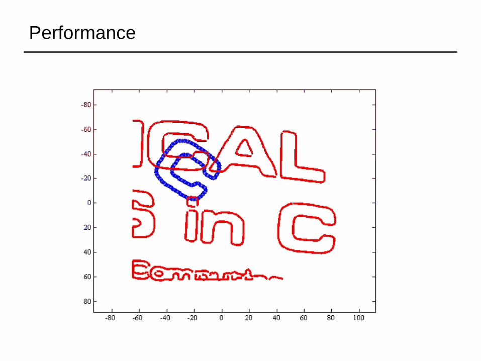
Performance

Unconstrained univariate optimization

We will look at three basic methods to determine the minimum:

1. gradient descent

2. polynomial interpolation

3. Newton’s method

These introduce the ideas that will be applied in the multivariate case

minx

f ( x)

f ( x)

For the moment, assume we can start close to the global minimum

A typical 1D function

As an example, consider the function

(assume we do not know the actual function expression from now on)

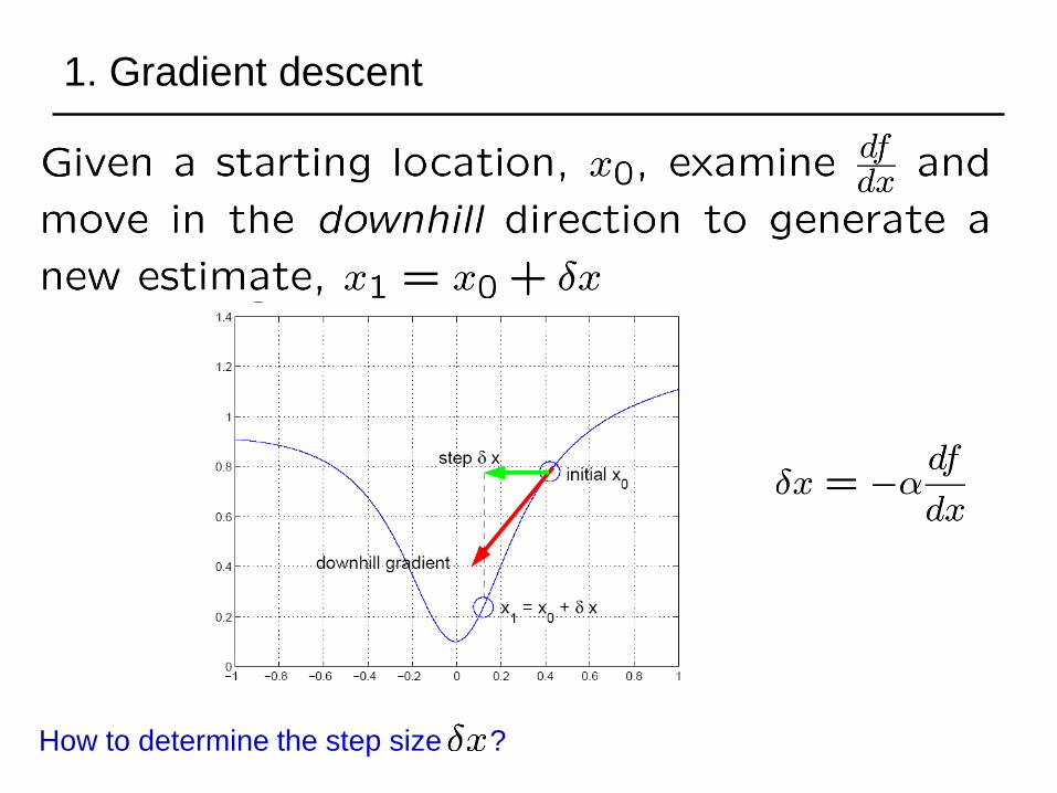
1. Gradient descent

How to determine the step size ?

2. Polynomial interpolation (trust region method)

-1 -0.8 -0.6 -0.4 -0.2 0 0.2 0.4 0.6 0.8 10

0.2

0.4

0.6

0.8

1

1.2

1.4

Approximate f(x) with a simpler function which reasonably

approximates the function in a neighbourhood around the

current estimate x. This neighbourhood is the trust region.

Quadratic interpolation using 3 points, 2 iterations

Other methods to interpolate a quadratic ?

• e.g. 2 points and one gradient

-1 -0.8 -0.6 -0.4 -0.2 0 0.2 0.4 0.6 0.8 10

0.2

0.4

0.6

0.8

1

1.2

1.4

3. Newton’s method

-0.2 -0.15 -0.1 -0.05 0 0.05 0.1 0.15 0.20

0.05

0.1

0.15

0.2

0.25

0.3

0.35

0.4

0.45

-1 -0.8 -0.6 -0.4 -0.2 0 0.2 0.4 0.6 0.8 10

0.2

0.4

0.6

0.8

1

1.2

1.4

Newton iterations detail with quadratic

approximations

• avoids the need to bracket the root

• quadratic convergence (decimal accuracy doubles at every iteration)

-1 -0.8 -0.6 -0.4 -0.2 0 0.2 0.4 0.6 0.8 1-1

-0.5

0

0.5

1

-1 -0.8 -0.6 -0.4 -0.2 0 0.2 0.4 0.6 0.8 10

0.2

0.4

0.6

0.8

1

1.2

1.4

• global convergence of Newton’s method is poor

• often fails if the starting point is too far from the minimum

• in practice, must be used with a globalization strategy which

reduces the step length until function decrease is assured

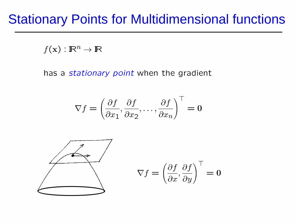
Stationary Points for Multidimensional functions

Extension to N dimensions

• How big can N be?

• problem sizes can vary from a handful of parameters to many

thousands

• In the following we will first examine the properties of

stationary points in N dimensions

• and then move onto optimization algorithms to find the

stationary point (minimum)

• We will consider examples for N=2, so that cost function

surfaces can be visualized

Taylor expansion in 2D

Taylor expansion in ND

Properties of Quadratic functions

At a stationary point the behaviour is determined by H

Examples of Quadratic functions

Case 1: both eigenvalues positive

-5 0 5 10 15-5

0

5

10

15

minimum

Case 2: eigenvalues have different signs

-5 0 5 10 15-5

0

5

10

15

saddle surface: extremum but not a minimum

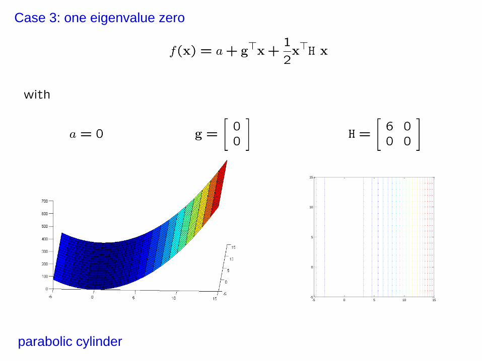
Case 3: one eigenvalue zero

-5 0 5 10 15-5

0

5

10

15

parabolic cylinder

Optimization in N dimensions – line search

• Reduce optimization in N dimensions to a series of (1D) line

minimizations

• Use methods developed in 1D (e.g. polynomial interpolation)

-5 0 5 10 15-5

0

5

10

15

An Optimization Algorithm

Reduces optimization in N dimensions to a series of (1D) line minimizations

Steepest descent

[exercise]

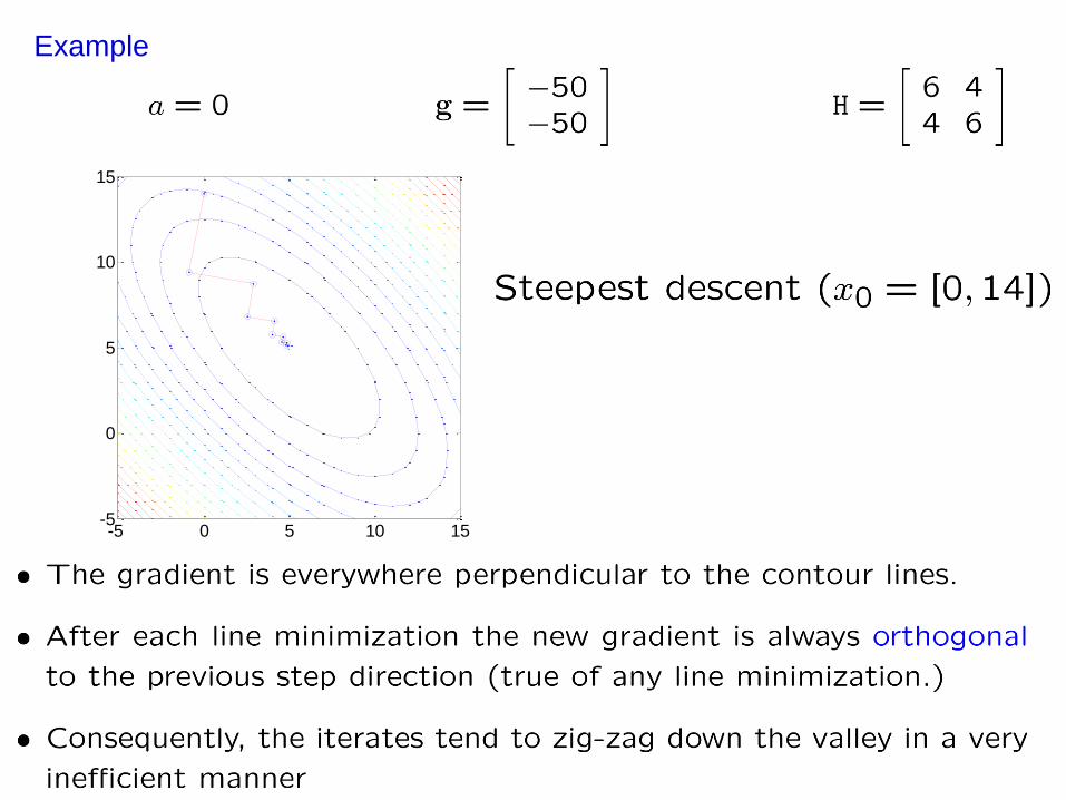
Example

-5 0 5 10 15-5

0

5

10

15

What is next?

• Move from functions that are exactly quadratic to general

functions that are represented locally by a quadratic

• Newton’s method (that uses 2nd derivatives) and Newton-

like methods for general functions