the geography of development - princeton universityerossi/gd.pdf · to the data for the whole world...

The Geography of Development

Klaus Desmet

Southern Methodist University

David Krisztian Nagy

Centre de Recerca en Economia Internacional

Esteban Rossi-Hansberg

Princeton University

We develop a dynamic spatial growth theory with realistic geography.We characterize the model and its balanced-growth path and proposea methodology to analyze equilibria with different levels of migrationfrictions. Different migration scenarios change local market size, inno-vation incentives, and the evolution of technology. We bring themodelto the data for the whole world economy at a 17 � 17 geographic reso-lution. We then use the model to quantify the gains from relaxing mi-gration restrictions. Our results indicate that fully liberalizing migra-tion would increase welfare about threefold and would significantlyaffect the evolution of particular regions of the world.

I. Introduction

An individual’s place of residence is essential in determining her produc-tivity, income, and well-being. A person’s location, however, is neither a

We thank Treb Allen, Costas Arkolakis, Maya Buchanan, Angus Deaton, GordonHanson,TomHolmes, Chang-TaiHsieh, ErikHurst, Steve Redding, Frédéric Robert-Nicoud, AndrésRodríguez-Clare, Jesse Shapiro, Joe Shapiro, Áron Tóbiás, Rob Townsend, and five refereesfor comments and discussions. We also wish to thank Adrien Bilal, Mathilde Le Moigne,

Electronically published May 7, 2018[ Journal of Political Economy, 2018, vol. 126, no. 3]© 2018 by The University of Chicago. All rights reserved. 0022-3808/2018/12603-0005$10.00

903

permanent characteristic nor a fully free choice. People tend to flee un-desirable and low-productivity areas to go to places that offer better op-portunities, but these choices are often hindered by an assortment ofrestrictions. An obvious example is the effort to stop undocumented mi-gration to Europe, theUnited States, andmost developed countries. Howdo these restrictions affect the evolution of the world economy? How dothey interact with today’s production centers, as well as today’s most de-sirable places to live, to shape the economy of the future? Any attempt toanswer these questions requires a theory of development that explicitlytakes into account the spatial distribution of economic activity, themobil-ity restrictions and transport costs associated with it, and the incentivesfor innovation implied by the world’s economic geography.Once wehavea basic understanding of the role of geography in development, we canstart evaluating the impact of events that change this geography.Constructing a theory to study the effect of geography on development

requires incorporating some well-known forces as well as others that havereceived, so far, less attention. First, a particular location is unique be-cause of where it is relative to other locations, which determines its costsof trading goods. Furthermore, each location has particular amenitiesthat determine its desirability as a place to live and a particular productiv-ity level that determines its effectiveness as a place to produce and work.This singularity of individual places underscores the importance of bring-ing the actual geography of the world, asmeasured by the location of landand water, as well as the distribution of other local spatial and economiccharacteristics, into the analysis. Second, migration across and withincountries is possible but limited, partly because of institutional restrictionsand partly because of social norms and other mobility costs. National bor-ders restrain mobility well beyond the existing frictions within countries,but frictions within countries are also potentially large. Third, the distinctlevels of labor productivity of locations, which reflect their institutions,infrastructure, education systems, and capital stocks, as well as location-specific technological know-how, evolve over time. Firms can invest in im-proving this local technology and infrastructure. Their incentives to do sodependon the size of themarket towhich they can sell their products. Thismarket size is determined by the magnitude of transport costs and the lo-cation’s geography relative to the potential customers of the product. Notall improvements in technology are local in nature or are the result of pur-poseful investments, though. Firms also benefit from the diffusion of theinnovations and creativity of others. Fourth, a location’s population den-sity affects its productivity, its incentives to innovate, and, perhapsmost im-portant, its amenities. Large concentrations of people in, for example, ur-

Charly Porcher, andMaximilian Vogler for excellent research assistance. Data are providedas supplementary material online.

904 journal of political economy

ban areas benefit from agglomeration effects but also suffer the undesir-able costs from congestion.Our aim is to study the evolution of the world economy at a rich level of

geographic detail (17 � 17 resolution) over many years. So our analysisnaturally involves many choices and compromises. The basic structureof themodel is as follows. Each 17� 17 cell of the world contains firms thatproduce a variety of goods using location-specific technologies that em-ploy labor and a local factor we refer to as land. Firms can trade subjectto iceberg transport costs. Each location is endowed with amenities thatenhance the quality of life in that cell. Agents have stochastic idiosyncraticlocational preferences drawn independently every period from a Fréchetdistribution. The static spatial equilibrium resembles the one proposedin Allen and Arkolakis (2014), but with migration, local factors, a tradestructure à la Eaton and Kortum (2002), and heterogeneous preferencesas in Kline and Moretti (2014).1 The dynamic model uses this structureand allows firms to invest in improving local technology as in Desmetand Rossi-Hansberg (2014). Technological innovations depend on a loca-tion’s market size, which is a function of transport costs and the entirespatial distribution of expenditure. Local innovations determine next pe-riod’s productivity after taking into account that part of these technologiesdisseminate over space.We not only characterize the distribution of economic activity in the

balanced-growth path but are also able to compute transitions since, asin Desmet and Rossi-Hansberg (2014), the innovation decision can be re-duced to a simple static problem due to land competition and technolog-ical diffusion. Our ability to prove the uniqueness of the equilibrium, tocharacterize the steady state, to identify the initial distribution of ameni-ties, productivity levels, and migration costs in all locations, and to simu-late themodel, though novel, is importantly enhanced by the set of resultsin Zabreyko et al. (1975), first used in spatial models in the related staticand single-country model of Allen and Arkolakis (2014). So we owe a sub-stantial debt to that work.Identifying the reasons why agents locate in a particular place necessar-

ily requires taking a stand on the opportunities they have to move acrosslocations in search of better living and work opportunities. Under the as-sumption of free mobility, a long tradition in urban and regional eco-nomics has identified productivity and amenities across locations usingland prices and population counts (see, e.g., Roback [1982] followingthe hedonic approach of Rosen [1979]). More recently, another strand

1 Since the Allen and Arkolakis (2014) framework is isomorphic to a setup with local fac-tors and a production and trade structure as in Eaton and Kortum (2002), the key differ-ence in the static part of the model is our introduction of migration costs.

the geography of development 905

of the literature has used income per capita and population counts, to-gether with a spatial equilibriummodel, to identify these same local char-acteristics (see, amongmany others, Desmet and Rossi-Hansberg [2013],Allen and Arkolakis [2014], Fajgelbaum and Redding [2014], and Beh-rens et al. [2017]).We follow this second strand of the literature but note that the static

nature of these papers yields a decomposition that depends crucially onparameters that are likely to evolve with the level of development of theeconomy. That is, the parameters used to identify amenities and pro-ductivities depend on the particular time period when the exercise wasdone. As a result, they do not represent stable parameters that one canuse to obtain meaningful conclusions in a dynamic context. In fact, inour theoretical framework, the relationship between income, populationdensity, and amenities evolves over time as the economy becomes richerand slowly converges to a balanced-growth path. We provide empirical ev-idence consistent with these theoretical patterns, using data from differ-ent regions of the world, as well as from US counties and zip codes.Another problematic assumption in this literature is free mobility, par-

ticularly becausewe are analyzingnot onlymigration across regions withina country but also migration across all countries in the world. While theassumption of freemobility within countries is clearly imperfect, althoughperhaps acceptable in some contexts, it is hard to argue that people any-where can freely move to the nicest and most productive places on earth.To see this, it suffices to have a casual look at the United States–Mexico bor-der or the restrictions on African immigration in Europe. More important,ignoring mobility restrictions leads to unreasonable conclusions. Take theexample of the Democratic Republic of the Congo, a country with the samepopulationdensity as theUnited States but with real wages that are orders ofmagnitude lower. The only way in which standard economic geographymodels with free mobility can reconcile this fact is to assume that Congohas some of the best amenities on earth. Even though it is hard to take a de-finitive stand on what characteristics a country’s individuals enjoy the most,and the heterogeneity in their preferences, basic evidence on health, edu-cation, governance, and institutions suggests that such a conclusion masksthe fact that many people in Congo do not choose to live there, but insteadare trapped in an undesirable location. Thus, we incorporate migrationfrictions within and across countries in our analysis.Once we explicitly account for migration restrictions, and therefore

utility differences across space, we get amore nuanced picture. To under-stand why, note that our theory identifies amenities only relative to utilityat each location. Hence, in the absence of mobility restrictions, the largevalues of amenities relative to utility in Congo would show up as those re-gions having high amenity levels. But if the Congolese face high mobilitycosts, then the same large values of amenities relative to utility would


show up as Congo having a low utility level. Identifying the actual amenitylevels therefore involves incorporatingmore data. To do so, we use surveydata on Cantril ladder measures of subjective well-being from the GallupWorld Poll.The subjective well-being data are an evaluative measure that asks indi-

viduals to assess their lives on a ladder scale, from theworst possible to thebest possible life they can envision for themselves. Deaton (2008) andKahneman and Deaton (2010) argue that this measure correlates wellwith log income and does not exhibit a variety of well-known pathologiesthat afflict hedonic measures of subjective well-being or happiness. Wetherefore interpret this evaluative measure as giving us information onthe welfare of individuals. Still, we need to convert this ladder with 11 stepsinto a cardinal measure of the level of utility. To do so, we match the rela-tionship between the ladder measure and log income in the model and inthe data. Using the cardinal measures of utility together with the amenityto utility ratios, we can recover the actual level of amenities for each cell ofthe world. As an overidentification check, we find that these estimatedamenities correlate well with commonly used exogenousmeasures of qual-ity of life.2

We can then use the evolution of population in themodel together withdata on population counts in each location for two subsequent periodsto compute the cost of moving in and out of each location in the world.This identifiesmobility costs between all locations, both within and acrosscountries, as the product of an origin- and a destination-specific cost.These migration costs will be key to quantitatively assessing different mi-gration policies, such as keeping costs constant in the future or fully lib-eralizing mobility.We calibrate the rest of the model using data on the evolution of out-

put across countries and other information from a variety of sources. Wethen perform a number of experiments in which we simulate the transi-tion of the world economy to its balanced-growth path. The parameterswe estimate guarantee that the equilibrium is unique and that the econ-omy eventually converges to a balanced-growth path in which the geo-graphic distribution of economic activity is constant. The transition tothis balanced-growth path can, however, take very long. If current migra-tion frictions do not change, it takes about 400 years for the economy toreach its balanced-growth path. The protracted length of this transition isthe result of the sequential development of clusters due to the complexityof the world’s geography. During these 400 years the world experiences

2 This suggests that subjective well-being differences capture an essential part of utilitydifferences across countries, although both concepts are unlikely to exactly coincide (seealso Glaeser, Gottlieb, and Ziv 2016).


large changes. The world’s real output growth rate increases progressivelyto around 2.9 percent by 2100 and then decreases back to 2.8 percent, whilethe growth rate of welfare increases from around 2.4 percent to 2.8 percent.The correlation between GDP per capita and population density alsochanges dramatically. The world goes from the current negative correla-tion of around 2.41 to a high correlation of .65 in the balanced-growthpath.3 That is, in contrast to theworld today, wheremany densely populatedareas are poor, in the future the dense regions will be the wealthy regions.4

Before using our quantified framework as a tool to evaluate the role ofmigratory restrictions and potentially other spatial frictions, it is impor-tant to gauge its performance using data that were not directly used inthe quantification. For this purpose we develop a method to solve ourmodel backward, allowing us to compute the model-implied distributionof population in the past. We run the model backward for 130 years andcompare the country population levels and growth rates predicted by themodel to those in the Penn World Tables and Maddison (2001). The re-sults are encouraging. The model does very well in matching populationlevels, and it also performs quite well in matching population growthrates. For example, we find that the correlation of the population growthrates between 1950 and 2000 implied by themodel and those observed inthe data is more than .7. This number declines somewhat for other timeperiods, but themodel preserves predictive power, even going as far backas 1870, in spite of many historical shocks, such as World Wars I and II,not being included in the analysis.Relaxing migration restrictions leads to large increases in output and

welfare at impact. The growth rates of real GDP and welfare also unam-biguously increase in the balanced-growth path, with the magnitude ofthe effect depending on the degree of liberalization. With the current fric-tions, about 0.3 percent of people migrate across countries and about0.45 percent move across cells in a year today (which is matched exactlyby the model), with this percentage converging to zero in the balanced-growth path. If, instead, we drop all restrictions, so there is freemobility, atimpact 70.3 percent of the populationmoves across countries and 71.6per-cent across cells. In present discounted value terms, complete liberaliza-tion yields output gains of 126 percent and welfare gains of 306 percent.Although this experiment is somewhat extreme and we also compute theeffects of partial liberalizations, it illustrates the large magnitude of thegains at stake and it highlights the role of migration policies when thinkingabout the future of the world economy.

3 The correlation is computed using 17 � 17 land cells as units.4 Consistent with wealthy regions having a stronger correlation between population

density and income per capita, in 2000 the correlation was only 2.11 in Africa and as highas .50 in North America.


Different levels of migration restrictions put the world on alternativedevelopment paths in which the set of regions that benefit varies dramat-ically. With the current restrictions, we get a productivity reversal, withmany of today’s high-density, low-productivity regions in sub-Saharan Af-rica, South Asia, and East Asia becoming high-density, high-productivityregions, and North America and Europe falling behind in terms of bothpopulation and productivity. In contrast, when we relaxmigration restric-tions, Europe and the eastern areas of the United States remain strong,with certain regions in Brazil and Mexico becoming important clustersof economic activity too.The driving forces behind these results are complex since the world is

so heterogeneous. One of the key determinants of these patterns is thecorrelation between GDP per capita and population density. As we men-tioned above, the correlation is negative and weak today, and our theorypredicts that, consistent with the evidence across regions in the world to-day, this correlation will become positive and grow substantially over thenext six centuries, as the world becomes richer. Two forces drive this re-sult. First, people move to more productive areas, and second, moredense locations become more productive over time since investing in lo-cal technologies in dense areas is, in general, more profitable. Migrationrestrictions shift the balance between these twomechanisms. Ifmigrationrestrictions are strict, people tend to stay where they are, and today’sdense areas, which often coincide with developing countries, becomethemost developed parts of the world in the future. If, in contrast, migra-tion is free, then peoplemove to themost productive, high-amenity areas.This tends to favor today’s developed economies. Liberalizing migrationimproves welfare so much because it makes the high-productivity regionsin the future coincide with the high-amenity locations. So relaxing migra-tion restrictions eliminates the productivity reversal that we observe whenmigration restrictions are kept constant.These results highlight the importance of geography, and the interac-

tion of geography with factor mobility, for the future development pathof the world economy. Any policy or shock that affects this geography canhavepotentially large effects through similar channels.One relative strengthof our framework compared to the current literature is that, by explicitlymodeling the evolution of local technology over time, it incorporates intothe analysis the effect of spatial frictions on productivity. By doing so, itaccounts for the future impact ofmigrants on local productivity and ame-nities, rather than for just their immediate impact on congestion and theuse of local factors. The resulting growth effects can be large, suggestingthat this interaction between spatial frictions and productivity should bean essential element in any analysis of the impact of migration restric-tions.


The rest of thepaper is organized as follows. Section II presents themodeland proves the existence and uniqueness of the equilibrium. Section IIIprovides a sufficient condition on the parameters for a unique balanced-growth path to exist. Section IV discusses the calibration of the model, in-cluding the inversion to obtain initial productivity and amenity values, themethodology to estimate migration costs, and the algorithm to simulatethe model. Section V presents our numerical findings, which include theresults for the benchmark calibration and the results for different levelsof migration frictions. Section VI presents conclusions. Appendix A pre-sents empirical evidence of the correlation of density and productivity, andit shows how our estimates of amenities correlate with exogenous measuresof quality of life. It also discusses the robustness of our results to changes indifferent parameter values. Appendix B presents the proofs not includedin the main text. Appendix C provides a summary of the data sources.Videos with simulations of the world economy for different migration sce-narios are available online.

II. The Model

Consider an economy that occupies a closed and bounded subset S ofa two-dimensional surface that has positive Lebesgue measure. A loca-tion is a point r ∈ S . Location r has land density H ðr Þ > 0, where H(⋅)is an exogenously given continuous function that we normalize so thatÐSH ðr Þdr 5 1. There are C countries. Each location belongs to one coun-try; hence countries constitute a partition of S: (S1, . . . , SC). The worldeconomy is populated by �L agents who are endowed with one unit of la-bor, which they supply inelastically. The initial population distribution isgiven by a continuous function �L0ðr Þ.

A. Preferences and Agents’ Choices

Every period agents derive utility from local amenities and from consum-ing a set of differentiated products according to constant elasticity of sub-stitution preferences. The period utility of an agent i who resides in rthis period t and lived in a series of locations �r2 5 ðr0, : : : , rt21Þ in all pre-vious periods is given by

uit �r2, rð Þ 5 at rð Þ

ð1

0

cqt rð Þrdq� �1=r

εit rð ÞYt

s51

m rs21, rsð Þ21, (1)

where 1=½1 2 r� is the elasticity of substitution with 0 < r < 1, at(r) de-notes amenities at location r and time t, cqt ðr Þ denotes consumption ofgood q at location r and time t, mðrs21, rsÞ represents the permanent


flow-utility cost of moving from rs21 in period s 2 1 to rs in period s, andεitðr Þ is a taste shock distributed according to a Fréchet distribution. Weassume that the log of the idiosyncratic preferences has constant meanproportional to Q and variance p2Q2=6 with Q < 1. Thus,

Pr εit rð Þ ≤ z½ � 5 e2z21=Q

:

A higher value of Q indicates greater taste heterogeneity. We assume thatεitðr Þ is independent and identically distributed (i.i.d.) across locations,individuals, and time.Agents discount the future at rate b, and so the welfare of an individual

i in the first period is given byotbtui

t ðr it2, r it Þ, where r it denotes her locationchoice at t, r it2 denotes the history of locations before t, and r i0 is given.Amenities take the form

at rð Þ 5 �a rð Þ�Lt rð Þ2l, (2)

where �aðr Þ > 0 is an exogenously given continuous function, �LtðrÞ is pop-ulation per unit of land at r in period t, and l is a fixed parameter, wherel ≥ 0.5 Thus, we allow for congestion externalities in local amenities as aresult of high population density, with an elasticity of amenities to popu-lation given by 2l.An agent earns income from work, wt(r), and from the local ownership

of land.6 Local rents are distributed uniformly across a location’s resi-dents.7 So if Rt(r) denotes rents per unit of land, then each agent receivesland rent income RtðrÞ=�LtðrÞ. Total income of an agent in location r attime t is therefore wtðr Þ 1 Rtðr Þ=�Ltðr Þ. Agents cannot write debt contractswith each other. Thus, every period agents simply consume their income,and so

uit �r2, rð Þ 5

at rð ÞQts51m rs21, rsð Þ

wt rð Þ 1 Rt rð Þ=�Lt rð ÞPt rð Þ εit rð Þ

5at rð ÞQt

s51m rs21, rsð Þ yt rð Þεit rð Þ,

where yt(r) denotes the real income of an agent in location r, and Pt(r)denotes the ideal price index at location r in period t, where

5 This is consistent with the positive value of l we find in our estimation, although thetheory could in principle allow for a negative number, in which case amenities would ben-efit from positive agglomeration economies.

6 We drop the i superscript here because all agents in location r earn the same income.7 See Caliendo et al. (2018) for alternative assumptions on land ownership and their im-

plications.


Pt rð Þ 5ð1

0

pqt rð Þ2r=ð12rÞdq

� �2ð12rÞ=r:

Every period, after observing their idiosyncratic taste shock, agents de-cide where to live subject to permanent flow-utility bilateral mobility costsm(s, r). These costs are paid in terms of a permanent percentage declinein utility. In what follows we letmðs, r Þ 5 m1ðsÞm 2ðr Þ, withmðr , r Þ 5 1 forall r ∈ S . These assumptions guarantee that there is no cost to staying inthe same place and that the utility discount frommoving from one placeto another is the product of an origin-specific and a destination-specificdiscount. Furthermore, these assumptions also imply thatm 1ðr Þ 5 1=m 2ðr Þ.Hence, amigrant who leaves a location rwill receive a benefit (or pay a cost)m1(r), which is the inverse of the cost (or benefit) m 2ðr Þ 5 1=m 1ðr Þ of en-tering that same location r. As a result, a migrant who enters a countryand leaves that same country after a few periods will end up paying theentry migration costs only while being in that country. This happens be-cause, although the flow-utility mobility costs are permanent, the cost ofentering is compensated by the benefit from leaving.Our theory focuses on net, rather than gross, migration flows, since lo-

cal population levels are what determines innovation and hence the evo-lution of the global economy. Important, these assumptions on migra-tion costs do not impose a restriction on our ability to match data onchanges in population. As we will later show, because the migration costbetween any pair of locations in the world consists of an origin- and adestination-specific cost, we can use observations on population levelsin each location for two subsequent periods to exactly identify all migra-tion costs. We summarize these assumptions in assumption 1.Assumption 1. Bilateral moving costs can be decomposed into an

origin- and a destination-specific component, so mðs, r Þ 5 m1ðsÞm 2ðr Þ.Furthermore, there are no moving costs within a location, so mðr , r Þ 51 for all r ∈ S .Independently of the magnitude of migration costs, preference het-

erogeneity implies that the elasticity of population with respect to real in-come adjusted by amenities is not infinite. This elasticity is governed bythe parameter Q, which determines the variance of the idiosyncratic pref-erence distribution. Conditional on a location’s characteristics, summa-rized by at(r)yt(r), a location with higher population has lower averageflow utility, since the marginal agent has a lower preference to live in thatlocation. In that sense, preference heterogeneity acts like a congestionforce, an issue we will return to later on.Assumption 1 implies that the location choice of agents depends only

on current variables and not on their history or the future characteristicsof the economy. The value function of an agent living at r0 in period 0,


after observing a distribution of taste shocks in all locations, �εi1 ; εi1ð⋅Þ,is given by

V r0,�εi1ð Þ 5 max

r1

a1 r1ð Þm r0, r1ð Þ y1 r1ð Þεi1 r1ð Þ 1 bE

V r1,�εi2ð Þm r0, r1ð Þ

� �� 5

1

m1 r0ð Þmaxr1

a1 r1ð Þm2 r1ð Þ y1 r1ð Þεi1 r1ð Þ 1 bE

V r1,�εi2ð Þm2 r1ð Þ

� �� 5

1

m1 r0ð Þ maxr1

a1 r1ð Þm2 r1ð Þ y1 r1ð Þεi1 r1ð Þ

� ��1 bE max

r2

a2 r2ð Þm2 r2ð Þ y2 r2ð Þεi2 r2ð Þ 1 V r2,�εi3ð Þ

m 2 r2ð Þ� ��

,

where the second and third lines use assumption 1. Hence, since½a1ðr1Þ=m 2ðr1Þ�y1ðr1Þεi1ðr1Þ depends only on current variables and tasteshocks, the decision of where to locate in period 1 is independent ofthe past history and future characteristics of the economy. That is, thevalue function adjusted for the value of leaving the current locationV ðr , εiÞ=m2ðrÞ (which is equal to V(r, εi)m1(r) by assumption 1) is indepen-dent of the current location r. This setup implies that the location deci-sion is a static one and that we do not need to keep track of people’s pastlocation histories, a feature that enhances the tractability of our frame-work substantially.Consistent with this, we can show that an individual’s flow utility de-

pends only on her current location and on where she was in period 0(which is not a choice). Using (1) and taking logs, the period t log utilityof an agent who resided in r0 in period 0 and lives in rt in period t is

~uit r0, rtð Þ 5 ~ut rtð Þ 2 ~m1 r0ð Þ 2 ~m 2 rtð Þ 1 ~εit rtð Þ,

where ~x 5 lnx and ut(r) denotes the utility level associated with local ame-nities and real consumption, so

ut rð Þ 5 at rð Þð1

0

cqt rð Þrdq� �1=r

5 at rð Þyt rð Þ: (3)

Note that ut(r) summarizes fully how individuals value the productionand amenity characteristics of a location. Hence, it is a good measureof the desirability of a location, and it will be one of the measures weuse to evaluate social welfare. However, it does not include the mobilitycosts incurred to get there or the idiosyncratic preferences of individualswho live there.As an alternative measure to evaluate social welfare, we include taste

shocks into our measure, while still ignoring the direct utility effects ofmigration costs. As we will argue, it is more meaningful to leave out mo-


bility costs because very often the lack ofmigration between two locationsreflects a legal impossibility of moving (as well as lack of information orex ante psychological impediments) rather than an actual utility cost oncethe agent has moved. Hence, including migration costs when evaluatingthe social welfare effects of liberalizing migration restrictions would tendto grossly overestimate the gains. To compute this alternativemeasure, sup-pose therefore that individuals move across locations assuming they haveto pay the cost m(⋅, ⋅) but that the ones that move get reimbursed for thewhole stream of moving costs ex post. Then the expected period t utilityof an agent i who resides in r is

E ut rð Þεit rð Þji lives in rð Þ

5 G 1 2 Qð Þm 2 rð ÞðS

ut sð Þ1=Qm 2 sð Þ21=Qds

� �Q

,(4)

where G denotes the gamma function. Section A in appendix B providesdetails on how to obtain this expression.We now derive expressions of the shares of people moving between lo-

cations. The density of individuals residing in location s in period t 2 1who prefer location r in period t over all other locations is given by

Pr ~ut s, rð Þ ≥ ~ut s, vð Þ 8 v ∈ Sð Þ 5 exp ~ut rð Þ 2 ~m2 rð Þ½ �=Qð ÞðS

exp ~ut vð Þ 2 ~m 2 vð Þ½ �=Qð Þdv

5ut rð Þ1=Qm 2 rð Þ21=Qð

S

ut vð Þ1=Qm 2 vð Þ21=Qdv:

(5)

This corresponds to the fraction of the population in location s thatmoves to location r,

‘t s, rð ÞH sð Þ�Lt21 sð Þ 5

ut rð Þ1=Qm 2 rð Þ21=QðS

ut vð Þ1=Qm 2 vð Þ21=Qdv, (6)

where ℓt(s, r) denotes the number of peoplemoving from s to r in period t(or that stayed in r for ℓt(r, r)) and �Lt21ðsÞ denotes the total populationper unit of land in s at t 2 1. The number of people living at r at time tmust coincidewith thenumber of peoplewhomoved there or stayed there,so

H rð Þ�Lt rð Þ 5ðS

‘t s, rð Þds:


Using (6), this equation can be written as

H rð Þ�Lt rð Þ 5

ðS


ut vð Þ1=Qm 2 vð Þ21=QdvH sð Þ�Lt21 sð Þds

5ut rð Þ1=Qm 2 rð Þ21=Qð

S

ut vð Þ1=Qm 2 vð Þ21=Qdv

�L:

(7)

B. Technology

Firms produce a good q ∈ ½0, 1� using land and labor. A firm using Lqt ðr Þ

production workers per unit of land at location r at time t produces

qqt rð Þ 5 fq

t rð Þg1zqt rð ÞLqt rð Þm

units of good q per unit of land, where g1, m ∈ ð0, 1�. A firm’s productivityis determined by its decision on the quality of its technology—what wecall an innovation fq

t ðr Þ—and an exogenous local and good-specific pro-ductivity shifter zqt ðr Þ. To use an innovation fq

t ðr Þ, the firm has to employnfq

t ðr Þy additional units of labor per unit of land, where y > g1=½1 2 m�.The exogenous productivity shifter zqt ðr Þ is the realization of a randomvariable that is i.i.d. across goods and time periods. It is drawn from aFréchet distribution with cumulative distribution function

F z, rð Þ 5 e2Tt rð Þz2v

,

where Ttðr Þ 5 ttðr Þ�Ltðr Þa, and a ≥ 0 and v > 0 are exogenously given.The value of tt(r) is determined by an endogenous dynamic process thatdepends on past innovation decisions in this location and potentially inothers, fq

⋅ ð⋅Þ.We assume that the initial productivity t0(⋅) is an exogenously given

positive continuous function. Conditional on the spatial distribution ofproductivity in period t2 1, tt21ð⋅Þ, the productivity at location r in periodt is given by

tt rð Þ 5 ft21 rð Þvg1

ðS

htt21 sð Þds� �12g2

tt21 rð Þg2 , (8)

where h is a constant such thatÐShdr 5 1 and g1, g2 ∈ ½0, 1�. If g2 5 1 and

population density is constant over time, this implies that the mean of


zqt ðr Þ is ft21ðr Þg1 times themean of zqt21ðr Þ.8 That is, the distribution of pro-ductivity draws is shifted up by past innovations, but with decreasing re-turns if g1 < 1. If g2 < 1, the dynamic evolution of a location’s technologyalso depends on the aggregate level of technology,

ÐShttðsÞds.9

Later we will see that assuming g1, g2 ∈ ð0, 1Þ helps with the conver-gence properties of the model since we can have local decreasing returnsbut economywide linear technological progress. If g2 5 1, the evolutionof local technology is independent of aggregate technology, and as wewill show below, in a balanced-growth path in which the economy is grow-ing, economic activity could end up concentrating in a unique point. Incontrast, if g1 5 g2 5 0, only the aggregate evolution of technology mat-ters, there are no incentives to innovate, and the economy stagnates.Across locations zqt ðr Þ is assumed to be spatially correlated. In particu-

lar, we assume that the productivity draws for a particular variety in a givenperiod are perfectly correlated for neighboring locations as the distancebetween them goes to zero. We also assume that at large enough distancesthe draws are independent. This implies that the law of large numbers stillapplies in the sense that a particular productivity draw has no aggregate ef-fects. Formally, let z q

t ðr , sÞ denote the correlation in the draws zqt ðrÞ andzqt ðsÞ and let d(r, s) denote the distance between r and s. We assume thatthere exists a continuous function s(d), where dðr , sðdÞÞ 5 d such thatlimd → 0z

qt ðr , sðdÞÞ→ 1. Furthermore, z q

t ðr , sÞ 5 0 for d(r, s) large enough.One easy example is having land divided into regions of positive area,where z q

t ðr , sÞ 5 1 within a region and z qt ðr , sÞ 5 0 otherwise.

8 To obtain the mean of the standard Fréchet distribution F ðzÞ 5 e2Tt z2v

, first write downthe density function f ðzÞ 5 vTtz2v21e2Tt z2v

. The mean is thenÐ ∞0 zf ðzÞdz 5

Ð ∞0 vTtz2ve2Tt z2v

dz.Remember that GðaÞ 5 Ð ∞

0 ya21e2ydy. Redefine Ttz2v 5 y, so that dy 5 2vTtz2v21dz. Substi-

tute this into the previous expression, so thatð0

∞

Ttvz2v

2vTtz2v21 e

2ydy 5

ð0

∞2 ze2ydy 5 T

1v

t

ð∞

0

y21ve2ydy 5 T

1v

tGv 2 1

v

� �,

where Tt 5 ttLat . If g2 5 1, we have tt 5 f

vg1

t21tt21. Assuming the labor force does notchange over time, we can write

Tt

Tt21

5tt

tt21

5 fvg1

t21,

so that Tt 5 fvg1

t21Tt21. Hence, the expectation is given by

E ztð Þ 5 T1vt G

v 2 1

v

� �5 f

g1

t21T1v

t21Gv 2 1

v

� �5 f

g1

t21E zt21ð Þ:9 The assumption that h does not depend on r or s implies that any location benefits

from any other location’s technology, irrespectively of their distance. We need this assump-tion to characterize the balanced-growth path of the economy in Sec. III. However, we notethat all the results in Sec. II, such as the existence and the uniqueness of the equilibrium,carry over to the case in which technology diffusion has a spatial scope. We examine therobustness of our numerical results to this case in Sec. D of app. A.


Since firm profits are linear in land, for any small interval with positivemeasure there is a continuum of firms that compete in prices (à la Ber-trand). Note that the spatial correlation of the productivity draws, as wellas the continuity of amenities and transport costs in space, implies thatthe factor prices and transport costs faced by these firms will be similarin a small interval. Hence, Bertrand competition implies that their pric-ing will be similar as well. As the size of the interval goes to zero, theseprice differences converge to zero, leading to an economy in which firmsface perfect local competition.Local competition implies that firms will bid for land up to the point at

which they obtain zero profits after covering their investment in technol-ogy, wtðr Þnfq

t ðr Þy.10 So even though this investment in technology affectsproductivity in the future through equation (8), the investment decisionat any given point can safely disregard this dependence given the absenceof future profits regardless of the level of investment. This implies thatthe solution to the dynamic innovation decision problem is identical toa sequence of static innovation decisions that maximize static profits.Firms innovate in order to maximize their bid for land, win the land auc-tion, and produce. This decision affects the economy in the future, butnot the future profits of the firm, which are always zero. The implication,as discussed in detail in Desmet and Rossi-Hansberg (2014), is that weneed to solve only the static optimization problemof the firm and can dis-regard equation (8) in the firm’s problem.Therefore, after learning their common local productivity draw, zqt ðr Þ,

a potential firm at r maximizes its current profits per unit of land bychoosing how much labor to employ and how much to innovate,

maxLq

t rð Þ,fqt rð Þ pq

t r , rð Þfqt rð Þg1zqt rð ÞLq

t rð Þm 2 wt rð ÞLqt rð Þ

2 wt rð Þnfqt rð Þy 2 Rt rð Þ,

where pqt ðr , r Þ is the price charged by the firm of a good sold at r, which is

equivalent to the price the firm charges in another location net of trans-port costs. The two first-order conditions are

mpqt r , rð Þfq

t rð Þg1zqt rð ÞLqt rð Þm21 5 wt rð Þ (9)

and

g1pqt r , rð Þfq

t rð Þg121zqt rð ÞLqt rð Þm 5 ywt rð Þnfq

t rð Þy21: (10)

So a firm’s bid rent per unit of land is given by

10 Because in any location there are many potential entrants with access to the sametechnology, the bidding is competitive. There is no need to be more specific about the auc-tion.


Rt rð Þ 5 pqt r , rð Þfq

t rð Þg1zqt rð ÞLqt rð Þm 2 wt rð ÞLq

t rð Þ2 wt rð Þnfq

t rð Þy,(11)

which ensures all firms make zero profits. Using (9) and (10) gives

Lqt rð Þm

5ynfq

t rð Þyg1

: (12)

Then total employment at r for variety q, �Lqt ðr Þ, is the the sum of produc-

tion workers, Lqt ðrÞ, and innovation workers, nfq

t ðr Þy, so

�Lqt rð Þ 5 Lq

t rð Þ 1 nfqt rð Þy 5 Lq

t rð Þm

m 1g1

y

� �: (13)

Note also that

Rt rð Þ 5 y 1 2 mð Þg1

2 1

� �wt rð Þnfq

t rð Þy, (14)

so bid rents are proportional and increasing in a firm’s investment intechnology, wtðrÞnfq

t ðr Þy, as we argued above.In equilibrium firms take the bids for land by others, and therefore

the equilibrium land rent, as given and produce in a location if theirland bid is greater than or equal to the equilibrium land rent. Hence,in equilibrium, in a given location, the number of workers hired per unitof land and the amount of innovation done per unit of land are identicalacross goods. We state this formally in the following result.Lemma 1. The decisions of how much to innovate, fq

t ðr Þ, and howmany workers to hire per unit of land, �Lq

t ðr Þ, are independent of the lo-cal idiosyncratic productivity draws, zqt ðr Þ, and so are identical acrossgoods q.Proof. Since in equilibrium Rt(r) is taken as given by firms producing

at r, the proof is immediate by inspecting (12), (13), and (14). QEDLemma 1 greatly simplifies the analysis, as it will provide us with a re-

lation between pqt ðr , r Þ and zqt ðr Þ similar to the one in Eaton and Kortum

(2002) in spite of firms being able to innovate. Combining the equationsabove yields an expression for the price of a good produced at r and soldat r :

pqt r , rð Þ 5 1

m

� �mny

g1

� �12mg1Rt rð Þ

wt rð Þn y 1 2 mð Þ 2 g1ð Þ� �ð12mÞ2ðg1=yÞ wt rð Þ

zqt rð Þ : (15)

To facilitate subsequent notation, we rewrite the above expression as

pqt r , rð Þ 5 mct rð Þ

zqt rð Þ , (16)


where mct(r) denotes the input cost in location r at time t, namely,

mct rð Þ ; 1

m

� �mny

g1

� �12mg1Rt rð Þ

wt rð Þn y 1 2 mð Þ 2 g1ð Þ� �ð12mÞ2ðg1=yÞ

wt rð Þ: (17)

It is key to understand that from the point of view of the individual firm,this input cost mct(r) is given. As a result, expression (16) describes astraightforward relation between the productivity draw zqt ðr Þ and theprice pq

t ðr , r Þ. As in Eaton and Kortum (2002), this is what allows us inthe next subsection to derive probabilistic expressions of a location’sprice distribution, its probability of exporting to other locations, andits share of exports.

C. Prices, Export Probabilities, and Export Shares

Let ςðs, r Þ ≥ 1 denote the iceberg cost of transporting a good from r to s.Then, the price of a good q, produced in r and sold in s, will be

pqt s, rð Þ 5 pq

t r , rð Þς s, rð Þ 5 mct rð Þς s, rð Þzqt rð Þ : (18)

We impose the following assumption on transport costs.Assumption 2. ςð⋅, ⋅Þ : S � S →R is symmetric.As we derive formally in appendix B, the probability density that a given

good produced in an area r is bought in s is given by

pt s, rð Þ 5 Tt rð Þ mct rð Þς r , sð Þ½ �2vðS

Tt uð Þ mct uð Þς u, sð Þ½ �2vdu all r , s ∈ S : (19)

The price index of a location s, as we also show in appendix B, is thengiven by

Pt sð Þ 5 G2r

1 2 rð Þv 1 1

� �2ð12rÞ=r ðS

Tt uð Þ mct uð Þς s, uð Þ½ �2vdu

� �21=v

: (20)

D. Trade Balance

We impose trade balance location by location since there is no mecha-nism for borrowing from or lending to other agents. Market clearing re-quires total revenue in location r to be equal to total expenditure ongoods from r. Total revenue at r is

wt rð ÞH rð Þ Lt rð Þ 1 nft rð Þy� 1 H rð ÞRt rð Þ 5 1

mwt rð ÞH rð ÞLt rð Þ,


where the last equality comes from (12), (13), and (14). As in Eaton andKortum (2002), the fraction of goods that location s buys from r, pt(s, r),is equal to the fraction of expenditure on goods from r, so that the tradebalance condition can be written as

wt rð ÞH rð Þ�Lt rð Þ 5ðS

pt s, rð Þwt sð ÞH sð Þ�Lt sð Þds all r ∈ S , (21)

where the superscript q can be dropped because the number of workersdoes not depend on the good a firm produces, and L can be replaced by�L because the proportion of total workers to production workers is con-stant across locations.

E. Equilibrium

We define a dynamic competitive equilibrium as follows.Definition 1. Given a set of locations, S, and their initial technology,

amenity, population, and land functions ðt0, �a, �L0,H Þ : S →R11, as wellas their bilateral trade and migration cost functions ς,m : S � S →R11,a competitive equilibrium is a set of functions ðut , �Lt , ft , Rt , wt , Pt , tt ,TtÞ : S →R11 for all t5 1, ... , as well as a pair of functions ðp ⋅

t , c ⋅tÞ : ½0, 1� �S →R11 for all t 5 1, ... , such that for all t 5 1, ... :

1. Firms optimize and markets clear. Namely, (9), (10), and (13)hold at all locations.

2. The share of income of location s spent on goods of location r isgiven by (17) and (19) for all r, s ∈ S .

3. Trade balance implies that (21) holds for all r ∈ S .4. Land markets are in equilibrium, so land is assigned to the highest

bidder. Thus, for all r ∈ S ,

Rt rð Þ 5 y 2 my 2 g1

my 1 g1

� �wt rð Þ�Lt rð Þ:

5. Given migration costs and their idiosyncratic preferences, peoplechoose where to live, so (7) holds for all r ∈ S .

6. The utility associated with real income and amenities in location ris given by

ut rð Þ 5 at rð Þ wt rð Þ 1 Rt rð Þ=�Lt rð ÞPt rð Þ

5 �a rð Þ�Lt rð Þ2l y

my 1 g1

wt rð ÞPt rð Þ for all r ∈ S ,

(22)

where the price index Pt(⋅) is given by (20).


7. Labor markets clear, soðS

H rð Þ�Lt rð Þdr 5 �L:

8. Technology evolves according to (8) for all r ∈ S .

In what follows we prove results under the following assumption.Assumption 3. �að⋅Þ, H(⋅), t0(⋅), �L0ð⋅Þ : S →R11, and m(⋅, ⋅), ςð⋅, ⋅Þ :

S � S →R11 are continuous functions.Assumption 3 implies that there is no discontinuity in the underlying

functions determining the distribution of economic activity in space.Since we canmake these functions as steep as we want at borders or othernatural geographic barriers, this assumption comes at essentially no lossof generality. We prove all the results below under this assumption. Ofcourse, for the quantification and calibration of the model we will usea discrete approximation. Similar results for existence and uniqueness,involving the exact same parameter restrictions we impose below, canbe established directly for the discrete case by adapting some of the argu-ments in Allen and Arkolakis (2014).We canmanipulate the systemof equations that defines an equilibrium

and, ultimately, reduce it to a system of equations that determines wages,employment levels, and utility, ut(⋅), in all locations. In a given period t,the following lemma characterizes the relationship between wages, utility,and labor density, conditional on �að⋅Þ, tt(⋅), �Lt21ð⋅Þ, ς(⋅, ⋅),m(⋅, ⋅),H(⋅), andparameter values. Appendix B presents all proofs not included in themain text.Lemma 2. For any t and for all r ∈ S , given �að⋅Þ, tt(⋅), �Lt21ð⋅Þ, ς(⋅, ⋅),

m(⋅, ⋅), and H(⋅), the equilibrium wage, wt(⋅), population density, �Ltð⋅Þ,and utility, ut(⋅) schedules satisfy equations (7), as well as

wt rð Þ 5 �w�a rð Þut rð Þ

� �2 v112v

tt rð Þ 1112vH rð Þ2 1

112v�Lt rð Þa211 l1

g1y2 12m½ �½ �v

112v (23)

and

�a rð Þut rð Þ

� �2v 11vð Þ112v

tt rð Þ2 v112vH rð Þ v

112v

� �Lt rð Þlv2 v112v a211 l1g1

y2 12m½ �½ �v½ �

5 k1

ðS

�a sð Þut sð Þ

� � v2

112v

tt sð Þ 11v112vH sð Þ v

112vς r , sð Þ2v

� �Lt sð Þ12lv1 11v112v a211 l1g1

y2 12m½ �½ �v½ �ds,

(24)

where k1 is a constant.


We now establish conditions to guarantee that the solution to the sys-tem of equations (7), (23), and (24) exists and is unique. We can provethat there exists a unique solution wt(⋅), �Ltð⋅Þ, and ut(⋅) that satisfies (7),(23), and (24) if

a

v1

g1

y≤ l 1 1 2 m 1 Q:

This condition is very intuitive. It states that the static agglomerationeconomies associated with the local production externalities (a=v) andthe degree of returns to innovation (g1=y) do not dominate the threecongestion forces. These three forces are governed by the value of thenegative elasticity of amenities to density (l), the share of land in produc-tion, and therefore the decreasing returns to local labor (1 2 m), and thevariance of taste shocks (Q). Of course, the condition is stated as a func-tion of exogenous parameters only. We summarize this result in the fol-lowing lemma.Lemma 3. A solution wt(⋅), �Ltð⋅Þ, and ut(⋅) that satisfies (7), (23), and

(24) exists and is unique if a=v 1 g1=y < l 1 1 2 m 1 Q. Furthermore,the solution can be found with an iterative procedure.The two lemmas above imply that we can uniquely solve for wt(⋅), �Ltð⋅Þ,

and ut(⋅) given the allocation in the previous period. For t5 0, using theinitial conditions t0(⋅) and �L0ð⋅Þ, we can easily calculate all other equilib-rium variables using the formulas described in the definition of the equi-librium. We can then calculate next period’s productivity t1(⋅) at all loca-tions using equation (8). Applying the algorithm in lemma 3 for everytime period then determines a unique equilibrium allocation over time.The following proposition summarizes this result.Proposition 1. An equilibrium of this economy exists and is unique

if a=v 1 g1=y ≤ l 1 1 2 m 1 Q.

III. The Balanced-Growth Path

In a balanced-growth path (BGP) of the economy, if one exists, all regionsgrow at the same rate. A BGPmight not exist; instead, all economic activ-ity might eventually concentrate in one point, or the economy may cyclewithout reaching a BGP. Given the evolution of technology in (8), thegrowth rate of tt(r) is given by

tt11 rð Þtt rð Þ 5 ft rð Þvg1

ðS

htt sð Þtt rð Þ ds

� �12g2

:

Hence, in a BGP in which technology growth rates are constant, sott11ðr Þ=ttðr Þ is constant over time and space and ttðsÞ=ttðr Þ is constantover time, the investment decision will be constant but different across


locations. Divide both sides of the equation by the corresponding equa-tion for location s, and rearrange to get

tt sð Þtt rð Þ 5

f sð Þf rð Þ

� � vg112g2

5�L sð Þ�L rð Þ

� � vg1½12g2 �y

,

where the second equality follows from (12) and where we drop the timesubscript to indicate that we refer to a variable that remains constant inthe BGP. We can then use (7), (24), and the labor market clearing condi-tion to derive an equation that determines the spatial distribution of ut(r)on the BGP. According to theorem 2.19 in Zabreyko et al. (1975), aunique positive solution to that equation exists if

a

v1

g1

y1

g1

1 2 g2½ �y ≤ l 1 1 2 m 1 Q: (25)

This condition is strictly more restrictive than the condition that guar-antees the existence and uniqueness of an equilibrium in lemma 1 sinceit includes an extra positive term on the left-hand side. It is also intuitive.On the left-hand side we have the two static agglomeration effects: ag-glomeration externalities (a=v) and improvements in local technologyfor today’s production (g1=y). The third term, which appears in the con-dition for the BGP only, is related to the dynamic agglomeration effectfrom local investments in technology as well as diffusion (g1=([1 2 g2]y)).In fact, without diffusion, when 1 2 g2 5 0, condition (25) is never satis-fied and there is no BGP with a nondegenerate distribution of employ-ment. On the right-hand side of condition (25) we have the parametersgoverning the three dispersion forces, namely, congestion through loweramenities (l), congestion through lower land per worker (1 2 m), anddispersion because of taste shocks (Q). So condition (25) simply says thatin order for the economy to have a unique BGP, the dispersion forceshave to be large enough relative to all agglomeration forces. Similarly, thecondition in lemma 1 says that dispersion forces have to be strong enoughrelative to static agglomeration forces in order for an equilibrium to exist.The difference is that an equilibrium can exist even if condition (25) is vio-lated since the dynamic agglomeration effect might lead economic activityto progressively concentrate in an area of measure zero.We summarize the result in the following lemma.Lemma 4. If a=v 1 g1=y 1 g1=½½1 2 g2�y� ≤ l 1 1 2 m 1 Q, then there

exists a unique balanced-growth path with a constant distribution of em-ployment densities �Lð⋅Þ and innovation f(⋅). In the BGP tt(r) grows at aconstant rate for all r ∈ S .The condition that determines tt(r) in the BGP (which we write explic-

itly in the proof of lemma 4) guarantees that in the BGP welfare growsuniformly everywhere at the rate


ut11 rð Þut rð Þ 5

tt11 rð Þtt rð Þ

� �1=v

:

We can then use the equations above to show that the growth rate ofworld utility (or the growth rate of real output) is a function of the distri-bution of employment in the BGP.Lemma 5. In a balanced-growth path, under the conditions of lemma 4,

aggregate welfare and aggregate real consumption grow according to


ð1

0

cqt11 rð Þrdqð1

0

cqt rð Þrdq

26643775

1r

5 h12g2v

g1=n

g1 1 my

� �g1yðS

�L sð Þ vg1½12g2 �yds

� �12g2v

:

(26)

Hence welfare and aggregate real output growth depend on populationsize and its distribution in space.In a world with aggregate population growth the above result would re-

sult in strong scale effects in the BGP: growth of aggregate consumptionwould be an increasing function of world population in the BGP. There issome debate about whether such strong scale effects are consistent withthe empirical evidence. In particular, Jones (1995) observes that over thecourse of the twentieth century there has been no acceleration in thegrowth of income per capita in the United States in spite of an importantincrease in its population. Given that in our model the world economy isnot in the BGP and that population is constant, this issue is not of directconcern. However, if we were to allow for the world population to growover time, it would be straightforward to eliminate strong scale effectsin the BGP by making the cost of innovation an increasing function ofthe size of world population.11

IV. Calibration and Simulation of the Model

In order to compute the equilibrium of the model we need values for the12 parameters used in the equations above, in addition to values for ini-tial productivity levels and amenities for all locations, as well as bilateral

11 In particular, assume that to introduce an innovation fqt ðr Þ, a firm needs to employ

~nfqt ðrÞy�L units of labor per unit of land, where �L is total world population. This alternative

model is isomorphic to the benchmark model with n 5 ~n�L, and it implies a BGP growthrate of aggregate welfare and aggregate consumption that is no longer a function of theworld’s total population. In the alternative model, expression (26) would become a func-tion of �LðsÞ=�L rather than of �LðsÞ.


migration costs and transport costs between any two locations. Once wehave numbers for all of these variables and parameters, we can computethe model with the simple iterative algorithm described in the proof oflemma 3.Table 1 lists the parameter values and gives a brief explanation of how

they are assigned. When assigning parameter values, we assume a modelperiod to be 1 year, so we set b 5 0:965.12 We base some of the parametervalues on those in the existing literature. We estimate other parametervalues using ourmodel. In what follows we start by briefly discussing someof the parameter values that come from the literature and then provide adetailed discussion of how we estimate the remaining parameters.The elasticity of substitution, 1=ð1 2 rÞ, is set to 4, similar to the 3.8 es-

timated in Bernard et al. (2003). We choose a trade elasticity, v, equal to6.5, somewhere in the middle between the 8.3 value estimated by Eatonand Kortum (2002) and the 4.6 value estimated by Simonovska andWaugh (2014). The labor share in production, m, is set to 0.8.While higherthan the standard labor share, this parameter should be interpreted as thenonland share. Desmet and Rappaport (2017) find a land share of 0.1when accounting for the land used in both production and housing. Tak-ing a broader view of land by including structures, this share increases toaround 0.2, on the basis of a structures share slightly above 0.1, as cali-brated by Greenwood, Hercowitz, and Krusell (1997). We therefore takethe nonland share to be 0.8 but have checked that our main results are ro-bust to alternative values of this parameter.Equation (6) implies that Q is the inverse of the elasticity of migration

flows with respect to real income. In our specification, that elasticity is in-dependent of themigration costs as those are captured by our estimate ofm2. We therefore focus on elasticity measures estimated in contexts inwhich there are no formal migration restrictions. On the basis of thestudy by Ortega and Peri (2013), who look at intra-EU migration, as wellas Diamond (2016), Fajgelbaum et al. (2016), and Monte, Redding, andRossi-Hansberg (2018), who consider intra-US migration, a reasonablevalue for that elasticity is 2, so we set Q 5 0:5. In Section D of appen-dix A, we explore how our results depend on the particular value of Qby recomputing the model for a higher value.

12 We need to make individuals discount future consumption at a rate that is higher thanthe growth rate in the balanced-growth path. In our calibration, as well as in the differentcounterfactual scenarios with different migration costs, the growth rate of real consump-tion is never above 3.5 percent, so setting b 5 0:965 results in well-defined present dis-counted values in all our exercises.


TABLE1

ParameterValues

Param

eter

Targe

t/Commen

t

1.Preferences:o

tbt u

tðrÞ,whereutðr

Þ5�aðrÞ

Ltðr

Þ2lðrÞ

½Ð 1 0cq tðrÞ

rdq�1=r

andu0ðrÞ

5ew

~uðrÞ

b5

.965

Disco

untfactor

r5

.75

Elasticityofsubstitutionof4(B

ernardet

al.20

03)

l5

.32

Relationbetweenam

enitiesan

dpopulation

Q5

.5Elasticityofmigrationflowswithrespectto

inco

me(M

onte

etal.20

18)

w5

1.8

Deatonan

dStone(201

3)

2.Technology:qq tðrÞ

5f

q tðrÞ

g1zq tðrÞ

Lq tðrÞ

m,Fðz,

rÞ5

e2T

q tðrÞ

z2v

,an

dT

q tðrÞ

5t tðrÞ

Ltðr

Þa

a5

.06

Static

elasticity

ofproductivityto

den

sity

(Carlinoet

al.20

07)

v5

6.5

Tradeelasticity

(Eatonan

dKortum

2002

;Simonovska

andWau

gh20

14)

m5

.8Lab

orornonlandsharein

production(G

reen

woodet

al.19

97;Desmet

andRap

pap

ort

2017

)g15

.319

Relationbetweenpopulationdistributionan

dgrowth

3.Evolutionofproductivity:t tðrÞ

5f

t21ðrÞ

vg1½Ð S

ht t

21ðsÞ

ds�12

g2t t

21ðrÞ

g2an

dwðfÞ5

nfy

g25

.993

Relationbetweenpopulationdistributionan

dgrowth

y5

125

Desmet

andRossi-H

ansberg(201

5)n5

.15

Initialworldgrowth

rate

ofreal

GDPof2%

4.TradeCosts

ς rail5

.143

4ς n

o_rail5

.430

2ς m

ajor_road5

.563

6ς o

ther_road5

1.12

72Allen

andArkolakis(201

4)ς n

o_road5

1.97

26ς w

ater5

.077

9ς n

o_water5

.077

9U5

.393

Elasticityoftrad

eflowswithrespectto

distance

of2.93(H

eadan

dMayer

2014

)

A. Amenity Parameter

The theory assumes that a location’s amenities decrease with its popula-tion. As given by aðr Þ 5 �aðr Þ�Lðr Þ2l, the parameter l represents the elas-ticity of amenities to population. Taking logs gives us the following equa-tion:

log a rð Þð Þ 5 E log �a rð Þð Þð Þ 2 l log �L rð Þ 1 εa rð Þ, (27)

where Eðlogð�aðr ÞÞÞ is the mean of logð�aðr ÞÞ across locations, and εa(r) isthe location-specific deviation of logð�aðr ÞÞ from the mean. Assumingthat amenities are lognormally distributed across locations, we use datafrom Desmet and Rossi-Hansberg (2013) on amenities and populationfor 192 metropolitan statistical areas (MSAs) in the United States to esti-mate equation (27). One remaining issue is that not only does popula-tion affect amenities, but amenities also affect population. To deal withthis problemof reverse causality, we use anMSA’s exogenous productivitylevel as an instrument for its population. Desmet and Rossi-Hansbergprovide estimates for the exogenous productivity of MSAs, which they de-fine as the productivity that is not due to agglomeration economies. Whenusing this as an instrument, the identifying assumption is that a location’sexogenous productivity does not affect its amenities directly, but only indi-rectly through the level of its population. This is consistent with the as-sumptions of our model. Estimating (27) by two-stage least squares yieldsa value of l 5 0:32, which is what we report in table 1.

B. Technology Parameters

Our starting point is the economy’s utility growth equation in thebalanced-growthpath (26). To exploit the cross-country variation in growthrates in the data, assume that all countries are in a balanced-growth path,but their growth rates may differ.13 After taking logs and discretizing spaceinto cells, we can rewrite (26) for country c as

logut11 cð Þ 2 logut cð Þ 5 logyt11 cð Þ 2 logyt cð Þ5 a1 1 a2 logo

Sc

Lc sð Þa3 ,(28)

13 Essentially, we are assuming that the relative distribution of population within coun-tries has converged to what would be observed in a balanced-growth path, although inter-national migration flows may still change the relative distribution of population acrosscountries. As a result, growth rates may differ across countries, although each country ischaracterized by (26). As an alternative to this simplifying assumption, we could use thewhole structure of the model calibrated for 1990 and then estimate the parameters thatmake the simulated model match the observed growth rates. This calculation requiresenormous amounts of computational power and so is left for future research. The fact thatadding population growth to the estimating equation does not substantially change the re-sults alleviates this concern somewhat.


where a1 is a constant and

a2 51 2 g2½ �

v,

a3 5vg1

1 2 g2½ �y ,

and country-level per capita growth is such that, in a steady state,

logyt11 cð Þ 2 logyt cð Þ 5 logyt11 rð Þ 2 logyt rð Þfor all r ∈ c.14 The theory therefore predicts that steady-state growth is afunction of the following measure of the spatial distribution of popula-tion:

oS

L sð Þa3 : (29)

Assuming a2 > 0, then if 0 < a3 < 1, steady-state growth is maximizedwhen labor is equally spread across space; and if a3 > 1, steady-stategrowth is maximized when labor is concentrated in one cell. Before esti-mating (28), we normalize (29) in order to eliminate the effect of thenumber of cells differing across countries:

1

NSoS L sð Þa3 , (30)

where NS is the number of cells in a country. To see what this normaliza-tion does, consider two examples. Country A has four cells: two have pop-ulation levels L1 and two have population levels L2. Country B is identicalto country A but is quadruple its size: it has 16 cells, of which eight havepopulation levels L1 and eight have population levels L2. The above nor-malization (30) makes the population distribution measures of coun-tries A and B identical.To get empirical estimates fora1,a2, anda3, we use cell population data

fromG-Econ 4.0 to construct ameasure of (30) for four years: 1990, 1995,2000, and 2005. We focus on countries with at least 20 cells, and for thedata on real GDP per capita, we aggregate cell GDP and cell populationfrom the G-Econ data set to compute a measure of real GDP per capita.This gives us 106 countries and three time periods.

14 Equation (28) is consistent with there being no differences in population growthacross countries in a balanced-growth path. If we were to allow for such differences, thefirst part of expression (28) should be written as

logut11 cð Þ 2 logut cð Þ 5 logyt11 cð Þ 2 logyt cð Þ 2 l logLt11 cð Þ 2 logLt cð Þ½ �,where LtðcÞ ; oSc LtðsÞ. As we will discuss later, this leads to very similar parameter values.


When estimating (28), we use the between-estimator; that is, we use themean of the different variables. We do so because the dependent variable(growth) is rather volatile, whereas the independent variable of interest(the spatial distribution of population) is rather persistent. This suggeststhat most of the variation should come from differences between coun-tries rather than from differences within countries. Moreover, (28) is asteady-state relation, so focusing on the average 5-year growth rates seemssensible. Our estimation gives values of a2 5 0:00116 and a3 5 2:2. Us-ing the expressions for a2 and a3 following (28), this yields g1 5 0:319and g2 5 0:993, which are the values reported in table 1. Section D of ap-pendix Apresents some sensitivity analysis of our results to the strength oftechnological diffusion, given by 1 2 g2.If we were to allow for population growth, this would not affect the es-

timates as long as in the balanced-growth path population growth is thesame across countries. If, however, population growth rates do differacross countries, equation (28) would become

logyt11 cð Þ 2 logyt cð Þ 5 a1 1 a2 logoSc

Lc sð Þa3

1 l log Lt11 cð Þ 2 log Lt cð Þ½ �:

Reestimating this equation and imposing a value of l 5 0:32, as estimatedbefore, yields very similar results: a2 5 0:00103 and a3 5 2:6. This leavesthe values of g1 and g2 virtually unchanged at, respectively, 0.335 and0.993.Finally, we choose the level of innovation costs n so as tomatch a growth

rate of real GDP of 2 percent in the initial period. This yields a value ofn 5 0:15. We also need to choose a value for the static agglomeration ef-fect governed by a. Our model includes both static and dynamic agglom-eration effects, so we choose a relatively low value of a 5 0:06, which cor-responds to a static agglomeration effect of a=v 5 0:01. This value issimilar to, although a bit smaller than, the one estimated in Carlino,Chatterjee, and Hunt (2007) or Combes et al. (2012), since our modelalso features a dynamic agglomeration effect. In Section D of appen-dix A, we present a robustness test with a 20 percent larger value of a.

C. Trade Costs

We discretize the world into 17� 17 grid cells, which means 180 � 360 564,800 grid cells in total. A location thus corresponds to a grid cell. Toship a good from location r to s, one has to follow a continuous and once-differentiable path g(r, s) over the surface of the earth that connects thetwo locations. Passing through a location is costly. We assume that the costof passing through location r is given (in logs) by


log ς rð Þ 5 log ςrailrail rð Þ 1 log ςno_rail 1 2 rail rð Þ½ �1 log ςmajor_roadmajor_road rð Þ 1 log ςother_roadother_road rð Þ1 log ςno_road 1 2 major_road rð Þ 2 other_road rð Þ½ �1 log ςwaterwater rð Þ 1 log ςno_water 1 2 water rð Þ½ �,

where rail(r) equals one if there is a railroad passing through r and zerootherwise, major_road(r) equals one if there is a major road passingthrough r and zero otherwise, other_road(r) equals one if there is someother road (but no major road) passing through r and zero otherwise,and water(r) equals one if there is a major water route at r and zero oth-erwise. The coefficients ςrail, ςno_rail, ςmajor_road, ςother_road, ςno_road, ςwater, andςno_water are positive constants, and their values are based on values inAllenand Arkolakis (2014).We observe data on water, rail, and road networks at a finer spatial scale

than the 17 � 17 level. In particular, using data from http://www.naturalearthdata.com/, we can see whether there is a railroad, major road, andso forth passing through any cell of size 0.17 � 0.17. We aggregate thesedata up to the 17 � 17 grid cell level such that, for instance, rail(r) nowcorresponds to the fraction of smaller cells within cell r that have accessto the rail network. We do the same aggregation for the road and watervariables.15

Having ς(r), we use the Fast Marching Algorithm16 to compute the low-est cost between any two cells r ≠ s,

ς r , sð Þ 5 infg r ,sð Þ

ðg r ,sð Þ

ς uð Þdu� �U

,

whereÐg ðr ,sÞςðuÞdu denotes the line integral of ς(⋅) along the path g(r, s).17

15 Clearly, building roads and rail is endogenous to local development. We abstract fromthis aspect but note that major roads and rail lines are in general constructed through geo-graphically convenient locations, a feature of space that is, in fact, exogenous. In any case,the most important determinant of how costly it is to pass through a location is the pres-ence of water.

16 We apply Gabriel Peyre’s Fast Marching Toolbox for Matlab to search for the lowestcost, taking into account that the earth is a sphere. In particular, we adjust the values ofς(r) on the basis of the distance required for crossing a cell, which varies with the positionof the cell on the earth’s surface. We perform the Fast Marching Algorithm and calculatethese distances over a very fine triangular approximation of the surface.

17 We choose the trade cost of the cell with itself, ς(r, r), to equal the average cost be-tween points inside the cell,

E

ðg r1 ,r2ð Þ

ς rð Þdu� �

jr1, r2 ∈ r

� �U:

Note that these assumptions do not guarantee that all bilateral trade costs are above one.However, least-cost paths across cells and average least-cost paths within cells are longenough such that this is not a concern in the numerical implementation.


We calibrate U tomatch the elasticity of bilateral trade flows across cellsto distance in the data. In a meta-analysis of the empirical gravity litera-ture, Head and Mayer (2014) find a mean value of this elasticity equalto 20.93. We run a standard gravity regression on trade data simulatedby the model for the initial period and search for the value of U thatmatches this elasticity. This procedure identifies U uniquely since highervalues of Umust correspond to higher absolute values of the elasticity. Ityields U 5 0.393, implying that, conditional on the mode of transporta-tion, trade costs are concave in distance traveled. We also find that the re-sulting distance elasticity of within-country trade flows equals 21.32,which is very close to 21.29, the distance elasticity of trade flows acrosscounties within the United States estimated by Monte et al. (2018).Though we did not match it in the calibration, the simulation of the

world economy we present in the next section yields a ratio of trade toGDP in the world that is identical to the one observed in the data. We per-form robustness tests with respect to trade costs in Section D of appen-dix A.

D. Local Amenities and Initial Productivity

To simulate the model, we also need to know the spatial distribution of�aðr Þ and t0(r). We use data at the grid cell level on landH(r) from the Na-tional Oceanic and Atmospheric Administration, as well as population�L0ðrÞ and wages w0(r) as measured by GDP per capita in 2000 (period0) from G-Econ 4.0, to recover these distributions. Using equation (23)for t 5 0,

w0 rð Þ 5 �w�a rð Þu0 rð Þ

� �2 v112v

t0 rð Þ 1112vH rð Þ2 1

112v�L 0 rð Þa211 l1

g1y2 12m½ �½ �v

112v ,

we obtain

t0 rð Þ 5 �w2 112vð Þ �a rð Þu 0 rð Þ

� �v

H rð Þw0 rð Þ112v�L 0 rð Þ12a2 l1g1y2 12m½ �½ �v (31)

for any r. Plugging this into equation (24), we get

w0 rð Þ2v�L 0 rð Þlv �a rð Þu 0 rð Þ

� �2v

5 k1�w2 112vð Þ

ðS

w 0 sð Þ11v�L 0 sð Þ12lvH sð Þς r , sð Þ2v �a sð Þu0 sð Þ

� �v

ds:

(32)

Given H(r), �L0ðr Þ, and w0(r), we solve equation (32) for �aðr Þ=u 0ðr Þ. Wecan then use equation (31) to obtain t0(r). The following lemma shows


that the values of �aðrÞ=u 0ðr Þ and t0(r) that satisfy these equations areunique.Lemma 6. Given �w, the solution to equations (31) and (32) exists and

is unique.Proof. The existence and uniqueness of a solution to (31) directly fol-

low from the existence and uniqueness of a solution to (32). To prove ex-istence anduniqueness for (32), see theorem2.19 inZabreyko et al. (1975).QEDLemma 6 guarantees the existence and uniqueness of the inversion

of the model used to obtain �aðrÞ=u 0ðr Þ and t0(r). However, it does notguarantee that we can find a solution using an iterative procedure. In Sec-tion G of appendix B, we discuss the numerical algorithm we use to find asolution. Also, to solve for �aðr Þ=u 0ðr Þ and t0(r), we normalize �w to the av-erage wage in the world in 2000.The system above identifies �aðrÞ=u 0ðr Þ but is unable to tell �aðrÞ apart

from u 0(r). To disentangle a location’s amenity from its initial utility,we need to obtain an estimate of u 0(r). To do so we use data on subjectivewell-being from the Gallup World Poll. Subjective well-being is measuredon aCantril ladder from 0 to 10, where 0 represents the worst possible lifeand 10 the best possible life the individual can contemplate for herself.Thismeasure is, of course, ordinal, not cardinal. Furthermore, it requiresthe individual to set her own comparison benchmark when determiningwhat the best possible life, or the worst possible life, might mean. Thisbenchmark might vary across individuals, regions, and countries. How-ever, given that Deaton and Stone (2013) and Stevenson and Wolfers(2013) find a relationship between subjective well-being and the log ofreal income that is similar within the United States and across countries,we abstract from these potential differences in welfare benchmarks acrossthe world. But we still need to transform subjective well-being into a car-dinal measure of the level of well-being.Ignoring migration costs, recall that in the model the flow utility of an

individual i residing in location r is linear in her real income, namely,

ui rð Þ 5 a rð Þy rð Þεi rð Þ, (33)

where real income is yðrÞ 5 ½wðr Þ 1 Rðr Þ=�Lðr Þ�=Pðr Þ. Since we are focus-ing on a given timeperiod, we have dropped the time subscript in the pre-vious expressions. Then, to make the “ladder” data from the GallupWorld Poll comparable to the utility measure in the model, we need totransform subjective well-being into a measure that is linear in income.Deaton and Stone (2013) find that the ladder measure of the subjec-

tive well-being of an individual i residing in location r is linearly relatedto the log of her real income (see also Kahneman and Deaton 2010).In particular, they estimate a relation


�ui rð Þ 5 r lnyi rð Þ 1 v rð Þ 1 εiDS rð Þ, (34)

where the inverted hat refers to subjective well-being, as measured by theCantril ladder, v(r) is a location fixed effect, and εiDSðr Þ is a random vari-able with mean zero. Whereas the ladder measure is linear in the log ofreal income, our utilitymeasure in (33) is linear in the level of real income.To make (34) consistent with our model, we can rewrite (33) as18

r lnui rð Þ 5 r lnyi rð Þ 1 r lna rð Þ 1 r lnεi rð Þ: (35)

Equations (34) and (35) imply the following relation between utility asdefined in our model, ui(r), and utility as defined by subjective well-being, �uiðrÞ,

ui rð Þ 5 ew�ui rð Þ, (36)

where w 5 1=r. Given the structure of our model, one potential issuewith estimating (34) if we were to use only cross-country or cross-regionaldata is endogeneity: a location with a higher utility attracts more peopleand therefore affects the amenity levels through aðrÞ 5 �aðr Þ�Lðr Þ2l. How-ever, if (34) is estimated for a given time period using the cross-sectionalvariation and including location fixed effects, this is less of a concern.Using individual-level data, Deaton and Stone (2013) estimate r to bearound 0.55, which implies a value of w of 1.8. Our data on subjectivewell-being are at the country level, so we set u0ðr Þ 5 e1:8�uðcðrÞÞ, where �uðcðr ÞÞis the subjective well-being measure of the country c to which location rbelongs.Since the inversion has yielded estimates for �aðr Þ=u0ðr Þ, we can then

use the estimates of u0(r) to get a separate estimate for �aðr Þ. Because theestimates of u0(r) vary only at the country level, the data on subjectivewell-being are correcting only for the average utility level in a country,but not for the relative utility levels across regions within a country.19

E. Migration Costs

With initial technology and amenities at each location we can use dataon population levels in period 1 to estimate local migration costs. Equa-tion (7) implies that

18 For (34) and (35) to be completely consistent, we can rewrite lnaðr Þ 1 lnεiðrÞ in (35)as lna 0ðr Þ 1 lnε 0iðrÞ, where ln ε0 i(r) has mean zero. For this not to affect the subsequent es-timates of amenities, r ln a 0(r) must (up to a constant) be equal to r ln a(r). To guaranteethis, we assume that the distribution of taste shocks across individuals surveyed by the Gal-lup World Poll is identical across countries. Although theoretically these distributions mightbedifferent because of the selectionofmigrants, empirically this is unlikely to be an issue, giventhat only 3 percent of the world population lives outside their country of origin.

19 Of course, in subsequent periods ut(r) is allowed to vary freely within and across countries.


u1 rð Þ 5 H rð ÞQ�L1 rð ÞQ�L2Q

ðS

u1 vð Þ1=Qm 2 vð Þ21=Qdv

� �Q

m 2 rð Þ:

Plugging this into equation (24) that relates the period 1 population dis-tribution to amenities, land, and period 1 productivity and utility, we get

�a rð Þm 2 rð Þ

� �2v 11vð Þ112v

t1 rð Þ2 v112vH rð Þv1v 11vð ÞQ

112v

� �L1 rð Þlv2 v112v a211 l1g1

y2 12m½ �½ �v½ �1v 11vð ÞQ

112v

5 k1

ðS

�a sð Þm 2 sð Þ

� � v2

112v

t1 sð Þ 11v112vH sð Þv2v2Q

112v ς r , sð Þ2v

� �L1 sð Þ12lv1 11v112v a211 l1g1

y2 12m½ �½ �v½ �2 v2Q

112vds,

(37)

where

m2 rð Þ 5 m2 rð Þ�LQ

ðS

u1 vð Þ1=Qm2 vð Þ21=Qdv

� �2Q: (38)

The following lemma shows that, for a given continuous distribution of�að⋅Þ, t1(⋅),H(⋅), and �L1ð⋅Þ, there exists a unique solution to equation (37).Lemma 7. The solution to equation (37), m 2ð⋅Þ, exists, is unique, and

can be found by iteration.Proof. It follows from theorem 2.19 in Zabreyko et al. (1975) that the

solution exists and is unique if the ratio of the exponents on the right-hand side andon the left-hand side is not larger thanone in absolute value.It also follows from theorem 2.19 that iterating on the equation, we alwaysconverge to the solution if the ratio of the exponents is strictly smaller thanone in absolute value. Both conditions are automatically satisfied as

v2

1 1 2vv 1 1 vð Þ1 1 2v

5v

1 1 v< 1:

QEDThe solution to equation (37) yields a unique m 2ðr Þ for all r ∈ S . The

implied values of m2(⋅) are identified only up to a scale by equation (38).All equilibrium conditions depend on the distribution of m2(⋅) only, noton its level, so we simply normalize the level of m2(⋅) such that its mini-mum is equal to one. For interpretation purposes, entering any locationis costly relative to staying in one’s original location (and correspondingly,


leaving any location involves a gain due to assumption 1). Note that theseformulation and quantification of migration costs imply that everyone is“endowed” with the value of the location where they are born (or wheretheir family is located in the initial period). Of course, people born in amore desirable location obtain a larger “endowment” relative to peopleborn in less desirable places.To solve for m2(⋅), we need to know period 1 productivity and popula-

tion levels, t1(⋅) and �L1ð⋅Þ. We use the productivity evolution equation (8)to obtain t1(⋅) from t0(⋅) and �L0ð⋅Þ, while we use data on the populationdistribution in 2005 to obtain �L1ð⋅Þ.20

F. Simulations and Counterfactual Migration Scenarios

Once all parameters, as well as the functions �að⋅Þ, t0(⋅), m2(⋅), and ς(⋅, ⋅),are known, we can simulate the model forward by solving the system ofthree equations in lemma 3 to obtain ut(⋅), �Ltð⋅Þ, and wt(⋅) for every t 51, . . . . Every period we have to update the distribution of productivitiestt(⋅) using equation (8).We also want to calculate a set of counterfactual migration scenarios in

which we relax migration frictions in the world. To do so, we follow theprocedure above but use counterfactual migration frictions given by m2(⋅)ϑfor ϑ ∈ ½0, 1�. When ϑ 5 1, migration frictions are identical to the oneswe estimate in the data, so this case corresponds to keeping migrationfrictions unchanged. When ϑ 5 0, the counterfactual migration restric-tions imply that mðs, r ; ϑ 5 0Þ 5 1 for all s, r ∈ S , so that moving to anylocation in the world is free. We also calculate a variety of othermigrationscenarios in which we use values of ϑ strictly between zero and one. Notethat, relative to ϑ 5 1, an intermediate value of ϑ implies a distribution ofmigration costs with smaller differences across locations. Since we nor-malize m 2(⋅) by the minimum entry cost, we know that m2ðr Þ ≥ 1 for allr ∈ S . Hence, ϑ < 1 implies that we are decreasing the cost of enteringany destination. The value of ϑ can then be understood as an index ofthe severity of migration frictions in the world.

G. Backcasting

The procedure to simulate the model described in the previous sectionallows us to compute the distribution of economic activity over time start-ing from our base year, which we set to the year 2000. To gauge the per-formance of our model, we are also interested in simulating the model

20 We adjust for the discrepancy between the 5-year evolution in the data (from 2000 to2005) and the definition of a period as 1 year in our model by dividing population growthat each cell by 5. We also adjust all levels so that total population size remains unchanged.


backward in order to compute the implied distribution of populationin the past. This allows us to compare, as an overidentification test, thecorrelation between the past population data and the past distributionof population predicted by the model.Equation (7) allows us to express utility as a function of population and

moving costs,

ut rð Þ 5 m2 rð ÞH rð ÞQ�Lt rð ÞQðS

ut vð Þ1=Qm2 vð Þ21=Qdv

�L

26643775

Q

:

From equations (8), (12), and (13), productivity can be obtained as afunction of population and next period’s productivity, which yields

tt rð Þ 5 m 1 g1=y

g1=yn

� �vg1yg2

ðS

htt sð Þds� �12 1

g2

tt11 rð Þ 1g2 �Lt rð Þ2vg1

yg2 : (39)

Substituting these two equations in equation (24), we obtain

�a rð Þm2 rð Þ

� �2v 11vð Þ112v

H rð Þv1v 11vð ÞQ112v tt11 rð Þ2 v

g2 112vð Þ

� �Lt rð Þlv2 v112v a211 l1g1

y2 12mð Þ½ �v½ �1v 11vð ÞQ

112v 1 v2

112vg1yg2

5 ~kBt

ðS

�a sð Þm2 sð Þ

� � v2

112v

H sð Þv2v2Q112v tt11 sð Þ 11v

g2 112vð Þ

� �Lt sð Þ12lv1 11v112v a211 l1g1

y2 12mð Þ½ �v½ �2 v2Q

112v2v 11vð Þ112v

g1yg2ς r , sð Þ2vds,

(40)

where ~kBt does not depend on location. Given a set of continuous func-tions �að⋅Þ, H(⋅), m2(⋅), ς(⋅, ⋅), tt11ð⋅Þ, and the values of structural parame-ters, we can solve this equation, together with world labor market clearingÐS�LtðrÞdr 5 �L, to obtain the population distribution �Ltð⋅Þ. We can then

obtain tt(⋅) from equation (39). Using theorem 2.19 in Zabreyko et al.(1975), as before, the solution to equation (40) exists and is unique if

a

v2

g1

y

1

g2

2 1

� �≤ l 1 1 2 m 1 Q:

If the inequality is strict, we can find a solution using the same iterativeprocedure as the one described in the proof of lemma 3. Note that thiscondition is strictly weaker than the condition guaranteeing the exis-tence and uniqueness of an equilibrium in proposition 1, which is givenby a=v 1 g1=y ≤ l 1 1 2 m 1 Q, since g2 < 1. This result simply reflectsthat, since technology increases over time, dynamic agglomeration effects


are not an issue when running time backward. Hence, a backward predic-tion can be uniquely computed. We compare the outcome of this exercisewith historical data below.

V. The Geographic Evolution of the World Economy

This section has three aims. First, we want to enhance our understandingof the relation between space and growth. Ourmodel has predictions forthe future evolution of the spatial distribution of population and produc-tivity, as well as for the economy’s aggregate growth rate. Second, we wantto assess the accuracy of our model’s predictions for the spatial distribu-tion of population. To do so, we perform a backcasting exercise and com-pare its results with historical data. Finally, we want to understand the wel-fare impact of relaxing migration restrictions and how doing so changesthe distribution of economic activity in the balanced-growth path.

A. Benchmark Calibration

As explained in Sections IV.D and IV.E, we use cell-level data on land,population at two dates, wages, and trade costs to recover amenities, pro-ductivity, and mobility frictions. Whenever time-variant, the data aremostly for 2000 (see app. C for more details). All outcomes are plottedin natural logarithms. Figure 1 presents the results from the inversion ex-ercise with actual migration frictions to calculate the fundamental pro-ductivities and amenities. By “fundamental” we refer to the part of pro-ductivity and amenities that does not depend on population density.That is, it does not take into account the positive agglomeration econo-mies that benefit productivity and the negative congestion effects thathurt amenities. We also present the values of utility-adjusted amenitiesthat result directly from the inversion �aðr Þ=u0ðr Þ and the values of the en-try migration costs (m2(r)) that we identify from population movementsbetween years 2000 and 2005 as we described above.Fundamental productivity exhibits the expected patterns (see fig. 1A).

Productivity is generally high in North America, Europe, and Japan.When we look within countries, the main cities tend to display particularlyhigh levels of productivity. Mexico, for example, exhibits relatively lowproductivities, except for Mexico City and Monterrey. In China, Beijingand Shanghai have clearly higher fundamental productivities than the restof the country. This may reflect rules and regulations, as well as local edu-cational institutions that lead to higher-skilled populations. It is also wellknown that cities often tend to attract more productive workers. In thatsense it should not come as a surprise that urban areas stand out as placeswith high fundamental productivities. Clearly, sincewe are abstracting fromlocal capital investments, fundamental productivities also reflect the local


stock of capital, which tends to be larger in cities and, more broadly, in de-veloped economies.As for fundamental amenities (see fig. 1B), the highest values can be

found in South America and, in particular, Brazil. North America also en-joys high fundamental amenities, particularly in urban areas. In Europe,Scandinavia and the Netherlands exhibit high amenities, while Portugaland southern Europe fare worse. Thailand and southeastern Australiaare also desirable places to live, while some of the lowest amenities arefound in Africa and Siberia. In figure 1C we also present fundamentalamenities divided by the initial utility level, �aðr Þ=u 0ðr Þ. As we show inlemma 6, these values are the direct result of inverting the model usingpopulation and GDP per capita. Poor and densely populated areas havehigh values since the model rationalizes this combination of facts througheither high amenities or low utility associated with migration restrictions.Central Africa as well as large regions inAsia exhibit particularly high ratios.Comparing figures 1B and 1C, one can ascertain the role of initial utility-level differences due tomigration costs, which wemeasured using the sub-jective well-being data.

FIG. 1.—Benchmark calibration: results from the inversion and migration costs. A, Fun-damental productivities: t1(r ). B, Fundamental amenities: �aðr Þ. C, Amenities over utility:�aðr Þ=u 0ðr Þ. D, Migration costs: m2(r).


To validate our identification strategy for amenities, it is worthwhile tocorrelate our estimates of fundamental amenities with commonly usedexogenousmeasures of quality of life. We therefore collect data on differ-ent measures of geography (distance to oceans, distance to water, eleva-tion, and vegetation) and climate (precipitation and temperature). Thecorrelations between our estimates of amenities and these measures areconsistent with the literature. For example, we find that people like livingclose to water and prefer higher average temperatures and precipitation(Davis and Ortalo-Magné 2011; Albouy et al. 2016). Qualitatively, the re-sults do not depend on whether we look at all cells of the world, at onlycells in the United States, or at randomly drawn cells across countries.This suggests that ourmethodology of using data on subjective well-beingto identify amenities performs well. To further reinforce this point, pla-cebo correlations based on alternative identification strategies of ameni-ties yield correlations that are no longer the same across countries andwithin countries. Section B of appendix A presents these correlationsand provides further details.In figure 1D we present the measured entry migration costsm2(r). The

actual migration cost between s and r is given bym1(s)m2(r), which is equalto m2ðrÞ=m2ðsÞ as a result of assumption 1. Since we obtain these costs soas to exactly match population changes between two subsequent years inthe data, they should be interpreted as the total flow costs of entering aregion, including information and psychological costs, the cost of actu-ally getting there and settling there, and of course any legal migration re-strictions. The figure shows very large log values ofm 2(r) in many parts ofthe world, suggesting that a very large share of the migration costs likelyreflects legal impediments. It is hard to go to parts of Europe, particularlyScandinavia, parts of Canada and Alaska, Australia, New Zealand, andparts of the United States. One can distinguish the border between Mex-ico and theUnited States, Mexico andCentral America, as well as Finlandand Russia among others. Entering northern regions that are cold andhard to get to and settle is costly. Entering Africa, India, andChina, as wellas parts of Russia, is cheap. Overall these costs appear reasonable, butmore importantly, they make the model match exactly observed popula-tion flows. In the next section we show that they also imply past popula-tion distributions that compare well with historical data.Figure 2 (different panels) maps population, productivity, utility and

real income per capita. Following the theory, average productivity in eachcell is defined as ½ttðr Þ�Ltðr Þa�1=v. This productivity includes the positive lo-cal agglomeration effect and takes into account that each location drawsproductivities from a Fréchet distribution. In contrast to figure 1, theseare equilibriumoutcomes in the first period of themodel. Note that sinceu0(r) is based on our measure of subjective well-being and hence is con-


stant within countries, u1(r) also varies little within countries since the ad-justment takes place over a single year.Throughout this section we use ut(r) as our measure of utility since it is

a sufficient statistic of the characteristics of a location—real consumptionand amenities—that individuals value. Actual experienced utility also in-cludes the idiosyncratic preferences of individuals and possiblymigrationcosts (if not rebated). At the end of this section we compare the behaviorof these alternative measures of welfare.A first observation is that the correlation between population density

and productivity across countries is not that strong: there are some denselypopulated countries with high productivity levels, such as many of the Eu-ropean countries, but there are also some densely populated countrieswith low productivity levels, such as some of those located in sub-SaharanAfrica. Countries that are densely populated in spite of having low produc-tivity must have either low levels of utility (e.g., sub-Saharan Africa) or highlevels of amenities (e.g., Latin America).21 A second observation is that thesame relation between population density and productivity is much stron-ger across locations within countries, where thehigh-productivity areas typ-ically tend to be themetropolitan areas. This is not surprising since mobil-

FIG. 2.—Equilibrium in benchmark calibration (period 1). A, Population density. B,Productivity: ½ttðr Þ�Ltðr Þa�1=v. C, Utility: ut(r). D, Real income per capita: yt(r).

21 See also the map of the subjective welfare measures in Sec. C of app. A.


ity frictions tend to be smaller within countries, and so utility differencesacross locations within countries are relatively small. Thus, the negativecongestion effects from living in densely populated areas have to be com-pensated by either higher productivity or better amenities. In line with thisreasoning, we find that metropolitan areas have substantially higher pro-ductivity than the less dense neighboring locations, as well as somewhathigher, although less marked, real income per capita. The relatively highreal income in cities suggests that cities must enjoy lower amenity levelsdue to the negative effect of density on amenities. Diamond (2016) pro-vides empirical evidence on the importance of this effect.Now consider the evolution of this economy over time, when we keep

migratory barriers, as measured bym2(⋅), unchanged. Figure 3 (differentpanels) maps the predicted distributions of population, productivity,amenities, and real income per capita in period 600, at which point theeconomy has mostly converged to its balanced-growth path. Videos thatshow the evolution of these variables over time and over space are avail-able online. To visualize the changes over time, we should compare fig-ure 3, which represents the year 2600, with figure 2, which represents theyear 2000.Clearly, over time the correlation between population and productivity

across countries becomes much stronger. As predicted by the theory, in

FIG. 3.—Equilibrium keeping migratory restrictions unchanged (period 600). A, Popula-tion density. B, Productivity: ½ttðrÞ�LtðrÞa�1=v. C, Utility: ut(r). D, Real income per capita: yt(r ).


the long run, high-density locations correspond to high-productivity lo-cations. This can easily be seen when comparing the maps for period 1and period 600. While in period 1 the population and the productivitymaps look quite different, by period 600 they look very similar. As shownby the solid curve in panel B of figure 4, which presents the correlation ofpopulation density and productivity over time, the correlation increasesfrom around .38 in period 0 to 1.0 by period 600. Note, however, that thecorrelation between population density and real GDP, which is driven notonly by productivity but also by local prices, and therefore transport costsand geography, also grows but is never higher than .7. The solid curve inpanel A of figure 4 shows this. Since the correlation between productivityand population density grows faster than the correlation between outputand population density, panel C shows that the correlation between pro-ductivity and output exhibits a U-shaped pattern. Population respondsslowly to increases in productivity because of the presence of migrationrestrictions.The model’s prediction that the correlation between population den-

sity and income becomes stronger as the world becomes richer is presentin the data today. Although across all cells of the world the correlation to-day is negative, it is larger in wealthy regions. In 2000 the correlation be-tween population density and real income per capita was2.11 in Africa,.33 in western Europe, and .50 in North America. Similarly, in the UnitedStates the correlation is greater in high-income zip codes. In particular, in2000 the correlation between population density and income per capitawas .36 in zip codes with an income per capita above the median, com-pared to 2.06 in zip codes below the median. Section A of appendix Aprovides further details.Another remark is that the high-productivity, high-density locations

600 years from now correspond to today’s low-productivity, high-densitylocations, mostly countries located in sub-Saharan Africa, South Asia, andEast Asia. In comparison, most of today’s high-productivity, high-densitylocations in North America, Europe, Japan, and Australia fall behind interms of both productivity and population. Clearly, this is not the casein terms of welfare as measured by ut(r) (namely, amenity-adjusted realincomenot including eithermigration costs or idiosyncratic shocks), whereAmerica, Europe, and Australia remain strong throughout.This productivity reversal can be understood in the following way. The

high population density in some of today’s poor countries implies highfuture rates of innovation in those countries. Low inward migration costsand high outward ones imply that population in those countries increases,leading to greater congestion costs and worse amenities. As a result, to-day’s high-density, low-productivity countries end up becoming high-density, high-productivity, high-congestion, and low-amenity countries,whereas today’s high-density, high-productivity countries end up becoming


FIG.4.—

Correlationswithdifferentmigrationrestrictions.A,C

orrelationofln

y(r)

andln

L(r).B,C

orrelationofln(p

roductivity)

andln

L(r).C,C

or-

relationofln(p

roductivity)

andln

y(r).

medium-density, medium-productivity, low-congestion, and high-amenitycountries; theUnited States is among them.Australia’s case is somewhat dif-ferent since its low density and high inflow barriers imply that it becomes alow-productivity, high-amenity country. As canbe seen infigure 4, given thatthe correlation between population density, productivity, and real incomeper capita becomes relatively high, it must be that low-density, high-utilitycountries have high amenities.These dynamics imply a reallocation of population from high-utility to

low-utility countries, asmeasured by ut(r). Since the differences in amenity-adjusted real GDP are now smaller, idiosyncratic preferences compensatemore individuals to stay in areas with low ut(r). In principle this could bedriven by decreased migration from low- to high-utility countries or by in-creased migration from high- to low-utility countries. As increased innova-tion pushes up relative utility in low-income countries, fewer people wanttomigrate out, andmore people want tomigrate in, keeping relative utilitylevels about, although not completely, constant. Over time, this realloca-tion of population peters out. As predicted by lemma4, decreasing returnsto innovation, together with congestion costs, imply that, in the long run,the distribution of population reaches a steady state in which all locationsinnovate at the same constant rate.Most of our discussion so far has focused on the changing differences

across countries, but there are also interesting differences within coun-tries. When focusing on the population distribution within countries,we observe that as the population share of North America and Europe de-clines, the locations that better withstand this decline are the coastal ar-eas, which benefit from lower transport costs and thus higher real in-come. In the countries whose population shares are increasing, such asChina, India, and parts of sub-Saharan Africa, there is less evidence ofcoastal areas gaining. This movement toward the coasts is evident in allcountries when focusing on real GDP per capita, since coastal locationsare high-density, low-amenity locations (due to congestion) that havehigh market access and therefore more innovation.Figure 5 presents the average growth rates and levels of productivity,

real output, and welfare for different scenarios.22 The benchmark calibra-tion, which leaves mobility restrictions unchanged, corresponds to ϑ 5 1(solid curve).23 Consistent with the argument above, figure 5 shows thatthe average growth rates of productivity, real GDP per capita, and utilityconverge to constants after about 400 years. Note that the long-run growth

22 World average productivity at time t is defined asÐS ½H ðr Þ�Ltðr Þ=�L�½ttðrÞ�Ltðr Þa�1=vdr , i.e.,

the population-weighted average of locations’mean productivity levels. World average realGDP at t is defined analogously as

ÐS ½H ðr Þ�Ltðr Þ=�L�ytðr Þdr . World average utility is measured

asÐS ½H ðr Þ�LtðrÞ=�L�utðrÞdr , and it is based on the measure ut, which does not include migra-

tion restrictions or idiosyncratic preference shocks.23 We discuss the other curves in fig. 5. They represent alternative migration scenarios.


FIG.5.—

Growth

ratesan

dlevelsofproductivity,realGDP,an

dutilityunder

differentmigrationscen

arios.A,G

rowth

rate

ofproductivity.B,G

rowth

rate

ofreal

GDP.

C,Growth

rate

ofutility

(u).D,Lnworldaverageproductivity.E,Lnworldaveragereal

GDP.

F,Lnworldaverageutility

(u).

rate in real GDP per capita is higher than the initial growth rate, similar tothe pattern of utility growth. The growth rate of real GDP increases fromthe calibrated 2 percent in 2000 to about 2.9 percent and then slowly de-creases, to end slightly above 2.8 percent. Economic activity is more con-centrated in the balanced-growth path, leading to more investment andfaster growth. Productivity growth, in contrast, declines for the first 200 years,reflecting transitory losses from the initial population reallocation towardlow-productivity regions. From then on the spatial distribution of popula-tion density, �Ltð⋅Þ, changes little in this migration scenario. Finally, recallthat the growth rate in utility is equal to the growth rate in real GDP percapita minus l times the growth rate of population. Initially, the correla-tion between the growth in real GDP per capita and the growth in popula-tion is negative—many of the high-growth places in richer countries arelosing population—so that the growth rate in utility is greater than thegrowth rate in GDP per capita. In the long run, when the steady state isreached, there is no more reallocation of population across space, so thatrealGDPper capita, productivity, andutility grow at the same rates. Thebot-tom panels of figure 5 show the levels of world average productivity, realGDP, and utility as measured by ut.One of the forces that determine market size in themodel is the ability

to trade with other regions subject to transport costs. The level of trans-port costs determines the geographic scope of the area that firms con-sider when deciding how much to invest in innovation. In our frame-work, each cell trades with a group of other cells, within and acrosscountries. Recall that we parameterize trade costs such that we matchthe mean empirical estimate of the elasticity of bilateral cell-level tradeflows to distance (Head and Mayer 2014). We can also aggregate tradeat the country level in order to calculate the overall level of internationaltrade. The world trade share is calculated as

World Trade Sharet 5 1 2

ðS

ðc sð Þpt s, rð Þyt sð ÞH sð Þ�Lt sð Þdrdsð

S

yt sð ÞH sð Þ�Lt sð Þds,

where c(s) denotes the set of cells in the country of cell s. The second termdenotes the share of domestic consumption, where the numerator in-cludes the expenditure on domestic goods in the world and the denom-inator is total world GDP. In the simulation above, this trade share equals14.1 percent in 2000. Though not targeted by our model, this matchesthe actual ratio of trade to GDP in the world economy.24 Over time, the

24 According to the World Trade Organization, the ratio of exports plus imports to GDPin the world was 24 percent in 2000, increasing rapidly to 32 percent by 2008. One needs todivide these numbers by 2 to make them comparable to our statistic. This gives an averageshare of 14 percent over the 2000s, identical to the share in our benchmark calibration.


model predicts the trade share to increase slightly, reaching 15.1 percentby 2600. This upward trend is due to the emergence of high-productivityclusters in Africa, South Asia, and East Asia, all of which belong to differ-ent countries.Ourmodel incorporates both national and international trade barriers

and can be used to evaluate the overall effect of changes in trade costs. Inparticular, it can be used to measure both the static and dynamic gainsfrom trade. This is in contrast with most of the trade literature, which fo-cuses on static trade models without internal geography.25 Consider acounterfactual scenario that increases trade costs by 40 percent in thefirst period. Such a change reduces the trade share to 3.90 percent in pe-riod 1 and to 4.27 percent in the long run. The real GDP loss is 30.1 per-cent and the welfare loss, measured by ut, is 34.2 percent. These losses arean order of magnitude higher than the ones reported for static, one-sector, models in the survey by Costinot and Rodríguez-Clare (2014),who compute a real income loss from a similar change in trade costs of2.28 percent. Incorporating dynamic and within-country effects seemsto change the impact of trade frictions dramatically.

B. Predicting the Past

In this section we use the algorithmdescribed in Section IV.G to computethemodel’s implied population distribution in the past. Starting with thecalibration described in Section V.A for the year 2000, we run the simula-tion backward and compute the distribution of population in all cells ofthe world all the way back to the year 1870. We then compare the model-implied distribution to data from the PennWorld Tables 8.1 for every de-cade until 1950 and to data from Maddison (2001) for 1913 and 1870.These historic data are easily available at the country level, so we aggre-gate the cells in the model to the country level.This exercise is intended as an overidentification check for the model,

given that none of these historic population data were used in the quan-tification. Of course, there is a variety of world events and shocks that themodel does not incorporate, so it would be unreasonable to ask themodelto perfectly match the data. The model’s implications should be under-stood as the distribution of population that would result in the absenceof any forces and shocks not directly modeled. Examples of such un-modeled shocks abound: the two world wars, trade liberalization, decolo-nization, and so forth. With that caveat in mind, it is interesting to seehow much of the population changes the model can account for. Giventhat our framework attempts to model long-run forces driving populationchanges and growth, rather than short-term fluctuations and shocks, we

25 See, e.g., the survey in Costinot and Rodríguez-Clare (2014).


would expect themodel to performbest over themediumrun,when short-term shocks are less important, but the economy has not changed in fun-damental ways not modeled here.Table 2 reports the results. The model does very well: in levels, the cor-

relations back to 1950 are all larger than .96. Clearly, this is in large partdue to the fact that we match population levels in 2000 by construction,and population changes are not that large (about 3 percent per year).Hence, we also present the correlations of population growth rates. Thecorrelations for growth rates are clearly lower, but altogether still relativelyhigh. The correlation between the population growth rate from 1950 to2000 in the model and the data is .74. We view this as quite a success ofthe model. If we go all the way to 1870, the predictive power of the simu-lation is smaller, but the correlation of growth rates is still .34. In spite ofthe disruption of two world wars and many other major world events notaccounted for here, the model preserves substantial predictive power.

C. Evaluating Mobility Restrictions

We now analyze the effect of completely or partially relaxing existing mi-gration restrictions. We start with the free mobility scenario and then pre-sent some calculations for scenarios with partial mobility in which ϑ is be-tween one (current restrictions) and zero (free mobility).

1. Free Migration

In this exercise we evaluate the effects of completely liberalizing migra-tion restrictions. We start off with the benchmark calibration in period0 and then reallocate population such thatm2ðr Þ 5 1 for all r ∈ S , as cor-responds to the case with ϑ 5 0. For now, we take amenity-adjusted realGDP, ut(r), as our measure of a location’s utility. With free migration peo-plemove from locations with low ut to locations with high ut. This reducesutility differences across locations because of greater land congestionand lower amenities in high-utility locations (and the opposite in low-utility locations). This reallocation of population not only has a static ef-

TABLE 2Country-Level Population Correlations, 1870–2000: Model vs. Data

Year t

Penn World Tables 8.1 Maddison

1990 1980 1970 1960 1950 1913 1870

Correlation log population in t .993 .991 .982 .974 .965 .843 .681Correlation population growthfrom t to 2000 .414 .535 .504 .671 .742 .461 .344

Number of countries 152 131 131 102 53 76 76


fect but also has a dynamic effect by putting the economy on a differentdynamic path. As we have emphasized repeatedly, even thoughm2ðrÞ 5 1for all r ∈ S , differences in ut(r) are not eliminated, since idiosyncratictaste shocks imply that the elasticity of population to ut(r) is positivebut finite.Figure 6 and figure 7map the distributions of population, productivity,

utility, and real income per capita for period 1 and period 600, under theassumption that people are freelymobile across locations.26 Compared tothe exercise in which we kept migratory restrictions unchanged, severalobservations stand out. First, migration increases the initial correlationbetween population density and productivity across countries, so thatwe see fewer countries in which high density and low productivity coexist.In panel B of figure 4 we see that in the case of complete liberalization(ϑ 5 0) the initial correlation between density and productivity increasesfrom around .38 to nearly .69. Second, this initial effect has important dy-namic consequences. Because today’s poor countries lose populationthrough migration, they innovate less. As a result, and in contrast to the

26 For videos that show the gradual evolution over time and over space, see the onlineedition.

FIG. 6.—Equilibrium with free migration (period 1). A, Population density for ϑ 5 0. B,Productivity for ϑ 5 0: ½ttðr Þ�Ltðr Þa�1=v. C, Utility for ϑ 5 0: ut(r). D, Real income per capitafor ϑ 5 0: yt(r).


previous exercise, noproductivity reversal occurs between theUnited States,India, China, and sub-Saharan Africa. Third, this absence of a large-scaleproductivity reversal does not mean that relative productivities across coun-tries remain unchanged. Some countries, such as Venezuela, Brazil, andMexico, start off with relatively high utility levels but relatively low productiv-ity levels. This means they must have high amenities. Because of migration,they end up becoming some of the world’s densest and most productivecountries, together with parts of Australia, Europe, and the United States.Fourth, migration changes the determination of the development path ofthe world and thereby increases the growth rate in the balanced-growthpath, as is clear fromfigure 5. In the balanced-growthpath, realGDPgrowthincreases by about 0.5 percentage points. Fifth, within countries, there isstronger evidence of an increasing concentration of the population incoastal areas, compared to the benchmark case. The greater concentrationof population within countries, which was already apparent in the bench-mark case, is now reinforced by greater migration across countries. Sixth,the importance of coastal areas becomes even more apparent when welook at real income per capita. The fact that locations close to coastal areashave lower real income per capita but high population suggests that those

FIG. 7.—Equilibrium with free migration (period 600). A, Population density for ϑ 5 0.B, Productivity for ϑ 5 0: ½ttðr Þ�Ltðr Þa�1=v. C, Utility for ϑ 5 0: ut(r ). D, Real income percapita for ϑ 5 0: yt(r).


locations have higher amenities than the coastal areas themselves becauseof congestion.When analyzing the average growth in real income per capita and util-

ity, two differences become immediately apparent in figure 5 when com-paring the case of free migration (ϑ 5 0) to the case of no liberalization(ϑ 5 1). First, mobility increases the long-run growth rate of the econ-omy as well as the average level of welfare, output, and productivity inthe world. Second, growth in utility drops substantially in the short runas many people move to areas with high real GDP; hence these areas be-comemore congested and becomeworse places to live (lower amenities).This initial loss in growth is, however, compensated in the long run by alarge surge in productivity growth after year 2200.

2. Partial Liberalization

We now present the changes in discounted real income and welfare, aswell as migration flows, that result from a variety of scenarios in whichwe partially relax migration frictions. Figures 4 and 5 in the previous sec-tion already presented correlations as well as growth rates and levels ofthe different variables for an example scenario of partial liberalization,where we set ϑ 5 0:375.27 As can be seen in table 3, although this valueof ϑ is around themiddle between keeping existingmigration restrictionsunchanged and free migration, it leads to reallocations of populationthat are closer to the free migration case. When we liberalize migrationfully, 70.3 percent of the population changes country immediately; thecorresponding number when ϑ 5 0:375 is 52.7 percent. As expected,the share of population that moves decreases monotonically with themag-nitude of migration frictions as measured by ϑ.In terms of welfare, migration frictions are tremendously important,

particularly when we move closer to free migration.28 As shown in table 3,a liberalization that implies that about a quarter of the world populationmoves at impact (ϑ 5 0:75) yields an increase in real output of 30.6 per-cent. In terms of welfare, the increase depends on the measure we use.If, as we have done so far, we measure welfare as the present discountedvalue of the population-weighted average of u(r), the resulting welfare in-crease when we set ϑ 5 0:75 is 60 percent. This measure includes neitherthe mobility costs nor the idiosyncratic preference shocks. As we havenoted before, given that a large share of the migration costs are likely

27 We chose ϑ 5 0:375 to maximize visibility in the figures. Table 3 presents statistics formany other intermediate values of ϑ.

28 These calculations assume that the economy is on its balanced-growth path after pe-riod 600. Note in fig. 5 that in all cases the balanced-growth path growth rate remains strictlybelow 3.5 percent, and so, since b 5 0:965, the discounted present values of income andutility are well defined.


to derive from legal restrictions, accounting for the direct benefits fromlowering migration restrictions would tend to grossly overestimate thegains from liberalization.However, it mightmake sense to incorporate id-iosyncratic locational preferences into our welfare calculation. If we doso and calculate the value of the expected utility of agents as measured byequation (4), we obtain a welfare gain of 19.2 percent (as can be observedin col. 3 table 3 with heading E[uεi]). The second measure is naturallysmaller since agents are less selected when migration costs drop.Full liberalization that sets ϑ 5 0 leads to slightly less than three-quarters

of the world population migrating at impact and gives welfare gains, asmeasured by amenity-adjusted real GDP, of 305.9 percent and an increasein real income of 125.8 percent.29 Furthermore, if we take into accountidiosyncratic preference shocks, the gain is 79 percent. As explained be-fore, the welfare gains when taking into account locational preferencesare smaller because there is less selection under free mobility. These idio-syncratic preferences have sometimes been interpreted as capturing an-other type of mobility frictions. This is reflected in the elasticity of popula-tion tout being finite.When assessing the gains from freemigration, we arenot relaxing those implicit frictions.

29 To the best of our knowledge, this is the first paper to analyze the global gains frommobility in an endogenous growth model with spatial heterogeneity, costly trade, and ame-nities. Previous work that focuses on models with capital accumulation estimates long-rungains in income per capita of around 100 percent (Klein and Ventura 2007; Kennan 2013).Though not directly comparable to the present discounted numbers reported in table 3,we find somewhat larger effects. The main reason is that in our model mobility generatesboth a level and a long-run growth effect, whereas in these other models there is only alevel effect as the economy moves to its new steady state.

TABLE 3The Impact of Mobility Frictions

Mobility ϑ

Real Incomea

% D w.r.t. ϑ 5 1Welfare (u)b

% D w.r.t. ϑ 5 1

Expected WelfareE[uεi]c

% D w.r.t. ϑ 5 1Migration Flowsd

% D from t 5 0 to 1(1) (2) (3) (4)

1e 0 0 0 .30.875 13.8 26.4 9.1 10.0.750 30.6 59.8 19.2 21.2.500 69.2 144.3 40.5 43.2.375 87.1 188.8 50.3 52.7.250 101.6 228.8 58.9 60.2.125 113.2 264.5 67.3 66.00f 125.8 305.9 79.0 70.3

a Change in present discounted value (PDV).b Change in PDV of population-weighted average of cells’ discounted utility levels u(r).c Change of PDV of expected discounted utility levels as measured in eq. (4).d Net population changes in countries that grow divided by �L immediately after the

change in ϑ.e Observed restrictions.f Free mobility.


Two comments are in order when analyzing the numbers in table 3.First, themobility numbers presented in table 3 include agents whomoveacross countries at impact in period 1 only. Of course, as a result ofmigra-tory liberalization, the entire development path of the world economychanges significantly as shown in figures 4–7. Second, in general the gainsin utility as measured by amenity-adjusted real GDP are much larger thanthe gains in real income, especially when migration becomes freer. Relax-ing migration restrictions tends to relocate people to high-amenity re-gions. In the case of free migration, this reallocation accounts for nearly60 percent of the total welfare effect. Although the planner’s problem isintractable and unsolvable, this finding suggests what a planner mightwant to do. Given that our model implies that in the long run the high-productivity places will be the high-density places, ideally one would liketo see these high-density places in high-amenity places. Hence, a plannerinterested in maximizing long-run welfare would probably want to imple-ment policies that facilitate people moving to high-amenity places. Liber-alizing migration restrictions pushes the economy in that direction.Figure 8 presents growth rates of welfare using the two alternative mea-

sures. The figures in the first column simply reproduce the ones we pre-sented in figure 5; the ones in the second column present growth rates

FIG. 8.—Growth rates and levels with different migration restrictions. A, Growth rate ofutility (u). B, Growth rate of E[uεi]. C, Ln world average utility (u). D, Ln E[uεi].


and levels of welfare as measured by E[uεi] as in equation (4). With bothmeasures the growth rate of welfare is in general higher with freer migra-tion. Fluctuations over time in the growth rate of E[uεi] are a bit larger.Whenwe compare the levels of welfare, the twomeasures exhibit a similarbehavior.So far we have ignored the interaction between migration liberaliza-

tion and trade liberalization. Of course, the gains from lowering migra-tory barriers are likely to depend on the level of trade costs. To explorethis question, we compare the gains from free migration under differenttrade costs. In particular, we analyze how those gains change if we increasetrade barriers by 40 percent. Completely liberalizing migration increasesreal income by 125.8 percent if we leave trade restrictions unchanged,but those gains rise to 156.9 percent in a world with trade costs that are40 percent higher. The corresponding figures in terms of welfare, as mea-sured by amenity-adjusted real GDP, are 305.9 percent and 382.9 percent,respectively. The larger gains from free migration when trade costs arehigher suggest that trade and migration are substitutes: when trade is lessfree, the impact of liberalizing migration is larger.

VI. Conclusion

The complex interaction between geography and economic develop-ment is at the core of a wide variety of important economic phenomena.In our analysis we have underscored the fact that the world is intercon-nected through trade, technology diffusion, andmigration.We have con-ducted our analysis at a fine geographic detail, enabling us to incorporatethe significant heterogeneity across regions in amenities, productivity, ge-ography, and transport costs, as well as migration frictions. This frame-work and its quantification have allowed us to forecast the future evolutionof the world economy and to evaluate the impact of migration frictions.Our confidence in this exercise was enhanced by the model’s ability tobackcast population changes and levels, quite accurately, for many de-cades.Our results highlight the complexity of the impact of geographic char-

acteristics as well as the importance of their interaction with factor mobil-ity. We found that relaxing migration restrictions can lead to very largewelfare gains but that the world economy will concentrate in very differentsets of regions andnations depending onmigratory frictions. This inequityin the cross-country economic implications of relaxing migration frictionswill (and does) undoubtedly lead to political disagreements about theirimplementation. For example, developed economies today will guaranteetheir future economic superiority only in scenarios in which the world re-laxes migration restrictions. We have abstracted from these political econ-omy considerations, but they are clearly extremely important.


Even thoughour framework incorporates a large set of forces in a ratherlarge general equilibrium exercise, we had to make the choice of leavingsome important forces aside. Perhaps themost relevant one is the ability ofthe world economy to accumulate a factor of production like capital. Inour framework, only technology can be accumulated over time, not capi-tal. Inour view, theability of regions to invest in technology substitutes par-tially for the lack of capital accumulation, but clearly not fully. We also ab-stracted from local investments in amenities. In our framework, amenitiesvary only through changes in congestion as a result of in- or out-migration.Finally, we also abstracted from individual heterogeneity in education orskills. Given our long-term focus, we view educational heterogeneity as partof the local technology of regions. It is obviously the case that individualscanmigrate with their human capital, and we ignore this. However, the hu-man capital embedded in migrants lasts mostly for only one generation.Ultimately, migrants and, more important, their descendants will obtainan education that is commensurate with the local technology in a region.The framework we have proposed can be enhanced in the future to in-

corporate some of these other forces. However, as it already stands, it is auseful tool to understand the dynamic impact of any spatial friction. Wehave illustrated this using migration frictions, but clearly one could do alarge variety of other exercises. Two important ones that we hope we, orother researchers, will do in the future relate to climate change and tradeliberalizations. Both the international trade and the environmental liter-atures require a quantitative framework to understand the dynamic im-pact of environmental and trade policy that takes into account, and mea-sures, local effects. The quantitative framework in this paper is ready totake on these new challenges.

Appendix A

Density-Income Correlation and Subjective Well-Being

A. Correlation of Density and Income

In our theory, the presence of both static and dynamic agglomeration econo-mies, together with the role played by amenities, implies that the correlation be-tween density and income per capita is relatively low (and possibly negative)when income per capita is low and relatively high when income per capita is high.Two forces drive this result. On the one hand, the standard positive correlationbetween density and per capita income, due to static agglomeration economies,is stronger in high-productivity places that benefit from greater dynamic agglom-eration economies. This explains why the correlation between density and percapita income is increasing in per capita income. On the other hand, mobilitymeans that high-amenity places tend to have both high population density andlow per capita income. This explains why in relatively low per capita income lo-cations, where dynamic agglomeration economies are weak, the correlation be-


tween density and per capita income might be negative. To see whether thesefindings hold in the data, we provide evidence for the United States and theglobe.

Evidence from the United States.—For the United States we do two exercises. First,we compute the correlation between population density and income per workeracross US zip codes. We split zip codes into different groups: those with incomeper capita (worker) below themedian and those with income per capita (worker)above the median. The theory predicts a higher correlation between density andincome per capita for the latter group and possibly a negative correlation for theformer group. We also consider a finer split-up into four different groups by in-come per capita quartile. In that case, we would expect the correlation to increasewhen we go from lower income per capita quartiles to higher income per capitaquartiles.

Table A1 reports the results. Data on population, mean income per worker,and geographic area come from the 2000US census and from theAmericanCom-munity Survey 5-year estimates. The geographic units of observation are ZIP CodeTabulation Areas (ZCTAs).We use two different definitions of income: “earnings”correspond essentially to labor income, whereas “total income” also includes cap-ital income.As predictedby the theory, panelA shows that the correlation betweenpopulation density and earnings per full-time worker, both measured in logs, in-creases from .12 for ZCTAs with below-median earnings per full-time worker to.31 for ZCTAs above the median. When we focus on total income in panel B, theresults are similar, but now the correlation between population density and in-come per full-time worker is negative for ZCTAs below the median. In particu-lar, the correlation increases from 2.06 for those ZCTAs below the median to.36 for those above the median. All these correlations are statistically differentfrom zero at the 1 percent level, and in both cases, the increase in the correlationis statistically significant at the 1 percent level. When we compare different quar-tiles, rather than below and above the median, the results continue to be consis-tent with the theory: the correlations between density and income are greaterfor higher-income quartiles.

Second, we explore whether the relation between density and income is stron-ger in richer areas by analyzing how that relation at the zip code level changeswith the relative income of the Core Based Statistical Area (CBSA) the zip codepertains to. To analyze this, we start by running separate regressions for eachCBSA of the log of payroll per employee on the log of employee density at thezip code level. Using data of 2010 from the ZIP Code Business Patterns, this yields653 coefficients of employee density, one for each CBSA. Figure A1 then plotsthese 653 coefficients against the relative income of the CBSA. As expected, asthe relative income of the CBSA increases, the effect of employee density on pay-roll per employee increases.


TABLE A1Density and Income

Year

Percentiles Based on Mean Earnings

<25th 25th–50th 50th–75th >75th <Median ≥Median

A. Correlation Population Density (Logs) and MeanEarnings per Full-Time Worker (Logs)

2000 .0549*** .0884*** .1291*** .2199*** .1216*** .3128***2007–11 2.0237* .0428*** .1048*** .2727*** .0222*** .3546***

B. Correlation Population Density (Logs) and Per Capita Income (Logs)

2000 2.1001*** .0495*** .1499*** .2248*** 2.0609*** .3589***2007–11 2.0930*** .0175 .0733*** .2420*** 2.0781*** .3234***

* Significant at the 10 percent level.** Significant at the 5 percent level.*** Significant at the 1 percent level.

FIG. A1.—Payroll per employee and employee density

Rather than running separate regressions for each CBSA, we can also run asingle regression with an interaction term of density at the zip code level withpayroll per employee at the CBSA level:

y zipð Þ 5 a 0 1 a1d zipð Þ 1 a 2d zipð Þy cbsað Þ 1 ε zipð Þ, (A1)


where y(zip) is the log of payroll per employee at the zip code level, y(cbsa) is thelog of payroll per employee at the CBSA level, and d(zip) is the log of employeedensity at the zip code level. The theory predicts that a1 may be negative and thata2 is positive.Consistentwith this,whenusingdata from2010,wefinda1 5 20:241and a 2 5 0:079, and both are statistically significant at the 1 percent level. Usingdata from2000 yields similar results: a1 5 20:194 and a 2 5 0:075, andonce againboth are statistically significant at the 1 percent level.

Comparing different countries and regions.—Next we analyze the correlation be-tween real income per capita and population density across cells. Table A2 re-ports the results for different geographic subsets of the data. Across all cells ofthe world, the correlation between population density and real income per capitais2.41. Not surprisingly, within countries in which population mobility is higher,that correlation is positive and equal to .17. Of more interest is the comparisonbetween richer and poorer cells. We start by splitting up the world into the 50 per-cent poorest cells and the 50 percent richest cells. As expected, the correlationbetween population density and income per capita is lower for the poorer cells(2.06) than for the richer cells (.11). A similar ranking emerges when contrastingthe 50 percent poorest cells and the 50 percent richest cells within countries: thecorrelation is .16 for the poorer cells and .48 for the richer cells. Finally, we com-pare different continents and regions across the world. Once again, we would ex-pect the correlation between density and income per capita to be higher in moredeveloped regions. With the exception of Latin America, the results confirm thispicture: we see the lowest correlation in Africa (2.11) and the highest correla-tions in North America (.50) and in Australia and New Zealand (.70).

TABLE A2Correlation Population Density and Real Income

per Capita across Cells

1. Across all cells of the world 2.412. Weighted within-country average .173. Richest vs. poorest cells of the world:50% poorest cells 2.0650% richest cells .11

4. Richest vs. poorest cells within countries(weighted by number of cells per country):

50% poorest cells .1650% richest cells .48

5. Cell average within continents and regions:Africa 2.11Asia .06Latin America and Caribbean .18Europe .15Of which western Europe .33

North America .50Australia and New Zealand .70

B. Correlations of Amenities and Quality of Life

Our goal is to compute correlations between our estimated measures of funda-mental amenities and different exogenous measures of a location’s quality of


life. The different variables on quality of life, related to distance to water, eleva-tion, precipitation, temperature, and vegetation, come from G-Econ 4.0.30 Theresults are reported in table A3.

TABLE A3Correlations between Estimated Amenities and Different

Measures of Quality of Life

Correlations with Estimated Amenities (Logs)

All Cells United StatesOne Cell

per CountryPlacebo of

Col. 1Placebo of

Col. 3(1) (2) (3) (4) (5)

A. Water:Distance to ocean 2.3288*** .0544** 2.1102* 2.1277*** .3181***Distance to water 2.4894*** 2.3045*** 2.2054*** 2.3675*** .1638***Water < 50 km .2653*** .1731*** .1123* .1442*** 2.1428**

B. Elevation (logs):Level 2.4536*** 2.2116*** 2.2491*** 2.3151*** .2694***Standard deviation 2.4912*** 2.3018*** 2.2781*** 2.3597*** .2023**

C. Precipitation:Average .4301*** .1350*** .3860*** .3350*** .1016**Maximum .4462*** .1733*** .2383*** .4443*** .2992***Minimum .2279*** .2653*** .2150*** .0064 2.2613***Standard deviation .4126*** .0833*** .1969*** .4824*** .3954***

D. Temperature:Average .5920*** .7836*** .1123* .6832*** .4652***Maximum .5045*** .8141*** 2.0498 .6449*** .4034***Minimum .5867*** .7029*** .1621*** .6529*** .4131***Standard deviation 2.5455*** 2.3953*** 2.2438*** 2.5576*** 2.2983**

E. Vegetation:Desert, ice, or tundra 2.3553*** 2.4412*** 2.1771*** 2.2775*** 2.0919

* Significant at the 10 percent level.** Significant at the 5 percent level.*** Significant at the 1 percent level.

Column 1 presents correlations based on all 17 � 17 cells of the world. Thesecorrelations suggest that people prefer to live close to water, dislike high eleva-tions and rough terrain, like precipitation but not constantly, prefer warm andstable temperatures, and dislike deserts, tundras, and ice-covered areas. It is re-assuring that these correlations are largely consistent with those found in the lit-erature. For example, Albouy et al. (2016) provide evidence that Americans havea mild preference for precipitation and a strong preference to live close to water,and Davis and Ortalo-Magné (2011) find that there is a positive correlation be-tween quality of life and average temperature and precipitation. One thing thatmay come as a surprise is that people not only prefer higher average tempera-tures but also like higher maximum temperatures. This result is driven by the im-

30 All variables come directly fromG-Econ 4.0, but a couple require some further manip-ulation. In particular, the “distance to water” measure is defined as the minimum distanceto a major navigable lake, a navigable river, or an ice-free ocean; the different vegetationcategories in G-Econ can be found at http://data.giss.nasa.gov/landuse/vegeem.html.


posed linearity: once we allow for a quadratic relation between our measure ofamenities and maximum temperatures, we find an optimal maximum tempera-ture of 25.97 Celsius.

The fact that our correlations are overall in line with what we would expectsuggests that our methodology of identifying amenities by using data on subjec-tive well-being is reasonable. To further confirm this, we compare our results towhat these correlations would look like within the United States. Because utilityis the same across all cells within a country, the correlations within the UnitedStates do not depend on our use of data on subjective well-being. Hence, if theresults for the United States are similar to those of the world, this is further evi-dence in favor of ourmethodology. Column2 confirms that this is largely the case.

Another possible worry is that the correlations across all cells of the world aredriven by a few large countries. If so, what we observe in column 1 may mostly re-flect within-country variation, and this might explain why columns 1 and 2 looksimilar. To address this concern, we choose a random sample of 176 cells, onefor each country, and compute the correlations. We repeat this procedure5,000 times and report the resulting cross-country correlations in column 3. Theylook similar to those in columns 1 and 2.

As a further robustness check, we compute some placebo correlations to becompared with those in columns 1 and 3. To do so, we take a different value ofw when transforming subjective well-being into our measure of utility. In particu-lar, we assume that all countries in the world have the same utility when identify-ing fundamental amenities. The results are reported in columns 4 and 5. Notethat there is no need to run a similar placebo test on column 2 since the correla-tions within countries are independent of our measure of utility. Columns 4 and1 are similar. This is not surprising since most of the variation in those two col-umns is across cells within countries, and that variation is unaffected by the par-ticular value of w. In contrast, when we focus on the variation across countries,using a different value of w should change the results. This is indeed what we find:column 5 yields correlations very different from those in column 3. All the signson proximity to water and elevation have switched signs, and the correlation onminimum precipitation changes from positive to negative.

If the fundamental amenities that we have estimated are reasonable, then col-umns 1, 2, and 3 should yield similar results, columns 4 and 1 should not differmuch, and columns 5 and 3 should be quite different. Our results in table A3 con-firm these priors. Together with the fact that the correlations in column 1 are inline with those in the literature, this allows us to conclude that our particularmethodology of using subjective well-being to identify fundamental amenities per-forms well.


C. Subjective Well-Being

FIG. A2.—Cantril ladder measure of subjective well-being from the Gallup World Poll(max 5 10, min 5 0).

D. Robustness Exercises

We now conduct a number of robustness checks, related to different parameters.We study the effect of 20 percent changes in the parameters driving taste hetero-geneity (Q), static agglomeration economies (a), congestion in amenities (l), thedegree of technological diffusion (1 2 g2), the spatial span of technological dif-fusion (h), and the level of trade costs (U). All exercises keep the values of initialamenities, productivities, and migration costs, as well as other parameters, as inthe benchmark calibration. In addition to providing a quantitative assessment ofthe sensitivity ofourfindings to thesedifferentparameters, these robustness checksalso contribute to our understanding of the workings of themodel.

Preference heterogeneity.—In this exercise we increase Q, the parameter that de-termines preference heterogeneity, from0.5 to 0.6. The elasticity ofmigrant flowsto real income drops from 2 to 1.67. As a result, people are less likely to move tohigh-income or high-amenity places. This lowers the degree of spatial concentra-tion over time, so that growth rates go down in the long run (fig. A3). Relaxingmobility restrictions also has a smaller effect if people are less willing to move be-cause of stronger locational preferences. Consistent with this, table A4 shows a wel-fare gain of 243.0 percent from free mobility, compared to 305.9 percent in thebenchmark.


TABLE A4The Impact of Mobility Frictions

Real Income (%) Welfare (u) (%)a Welfare E[uεi] (%)b

ϑ 5 1 ϑ 5 0 ϑ 5 1 ϑ 5 0 ϑ 5 1 ϑ 5 0

1. Benchmark 0 125.8 0 305.9 0 79.02. Higher Q: .6 .1 109.6 4.6 258.7 499.3 703.7

109.4 243.0 34.13. Higher a: .072 2.8 132.9 2.6 319.9 2.3 84.4

126.6 309.4 80.44. Lower l: .256 1.0 176.6 142.8 1,476 115.6 459.3

174.0 549.1 159.45. Higher 1 2 g2: 1 2 .991 16.9 156.9 18.7 396.7 21.9 128.2

119.7 318.5 87.26. Local spatial diffusion 26.1 117.7 26.5 203.8 27.8 32.5

131.8 224.9 43.77. Trade costs 1 20% 217.3 97.0 220.0 251.0 223.7 47.2

138.3 338.9 93.08. Trade costs 1 40% 230.1 79.5 234.2 217.8 239.3 26.1

156.9 382.9 107.8

Note.—For each robustness exercise, the first line gives changes relative to the bench-mark with ϑ 5 1, while the second line gives gains from fully liberalizing migration.

a Change in PDV of population-weighted average of cells’ discounted utility levels, u(r).b Change of PDV of expected discounted utility levels as measured in eq. (4).

962

FIG.A3.—

Growth

ratesofreal

GDPan

dutility

fordifferentvalues

ofQ.A,Growth

rate

ofreal

GDP.

B,Growth

rate

ofutility

(u).C,Growth

rate

of

E[uεi].

963

Agglomeration economies.—Static agglomeration economies in our model aregiven by a=v. In the benchmark, with a 5 0:06 and v 5 6:5, the static elasticity ofproductivity to density was around 0.01. We now increase a by 20 percent to0.072. As expected, compared to the benchmark case, the present discounted val-ues of real income and welfare increase. We would expect this effect to be largerunder free mobility because it is easier to benefit from increased agglomerationeconomies when people can freely move. This is indeed the case: table A4 showsthat the gains in real income increase from 125.8 percent in the benchmark to126.6 percent, and the welfare gains increase from 305.9 percent in the bench-mark to 309.4 percent. Given that we increased the magnitude of static agglom-eration economies by 20 percent, the effects may seem modest. Note, however,that dynamic agglomeration economies aremore important in the long run thanstatic ones.

Congestion in amenities.—We now reduce the elasticity of amenities to density by20 percent. This drastically reduces congestion and hence makes it less costly toagglomerate. As a result, real income increases compared to the benchmark. Theeffects are larger under free mobility, when the possibility to concentrate in themost attractive places is enhanced. Greater concentration leads to faster growth,explaining why the increase in real GDP from free mobility rises from 125.8 per-cent in the benchmark to 174.0 percent (table A4). Not surprisingly, because thenegative congestion effect on amenities is much lower, the welfare gains are inrelative termsmuch greater. Freemobility now increases welfare by 549.1 percent.

Strength of technology diffusion.—In the model the degree of spatial diffusion oftechnology is given by 1 2 g2. In this exercise, we decrease g2 from 0.993 in thebenchmark to 0.991. This amounts to an increase in the degree of spatial diffu-sion of 20 percent.31 If best-practice technology diffuses faster, we would expectthis to increase growth. As can be seen in figureA4, this is indeed the case, but onlyunder current migration restrictions. In the case in which we eliminate movingcosts, after some decades of faster growth, more diffusion actually lowers growth.The reason is that greater diffusion of technology lowers the incentive to concen-trate in space. In the short run, the positive effect of more diffusion dominates,but in the long run the negative effect of less concentration and therefore less in-novation dominates. This reversal underscores the importance of dynamics whenthinking through the effect ofmore technological diffusion. Inpresent discountedvalue (PDV) terms, the effect of greater diffusion is positive on real income andwelfare gains. Since technological diffusion acts as a dispersion force, there is lesscongestion, so amenities improve. Stronger diffusion also implies that the econ-omy takes less time to reach its BGP, as can be seen from figure A4.

31 In order to eliminate the direct initial effect of the change in the level of technologydiffusion, we adjust the value of the constant h to match the initial growth rate of real GDPof 2 percent that we use in the benchmark calibration. Including this direct effect decreasesthe visibility of the graphs but does not lead to large changes in the gains from mobility,which are 109.9 percent in terms of real GDP, 256.8 percent in terms of utility, and 61.5 per-cent in terms of expected utility.


FIG.A4.—

Growth

ratesofreal

GDPan

dutility

fordifferentvalues

ofg2.A,Growth

rate

ofreal

GDP.

B,Growth

rate

ofutility

(u).C,Growth

rate

of

E[uεi].

Spatial scope of technology diffusion.—Though technology diffusion in the modelis slow, it diffuses to the whole world simultaneously. In this exercise, we explorewhat happens when we let technology diffuse locally rather than globally. In equa-tion (8), we no longer take h to be constant, but instead assume that hðr , sÞ 5�h expð2ϰdðr , sÞÞ, with ϰ > 0 and d(r, s) denoting the distance between locationsr and smeasured in kilometers. That is, location r obtains more technology spill-overs from nearby locations. On the basis of the median of the distance decay pa-rameters across different technologies in Comin, Dmitriev, and Rossi-Hansberg(2012), we use ϰ 5 0:0015. We choose the value of �h such that the initial growthrate of the economy is 2 percent as in the benchmark calibration; in other words,we change the geographic distribution of technology diffusion, but not its overalllevel. We present the results in figure A5. In the short run less spatial diffusionlowers growth rates, but in the long run it increases growth rates. To understandfigure A5 note that there are two effects at work. On the one hand, less spatial dif-fusion hurts some places, lowering growth. On the other hand, less spatial diffu-sion keeps economic activity more spatially concentrated, increasing innovation.In the short run, the first effect dominates, whereas in the long run the secondone does. Overall, going from global to local diffusion decreases real output andwelfare by about 7 percent as shown in table A4.


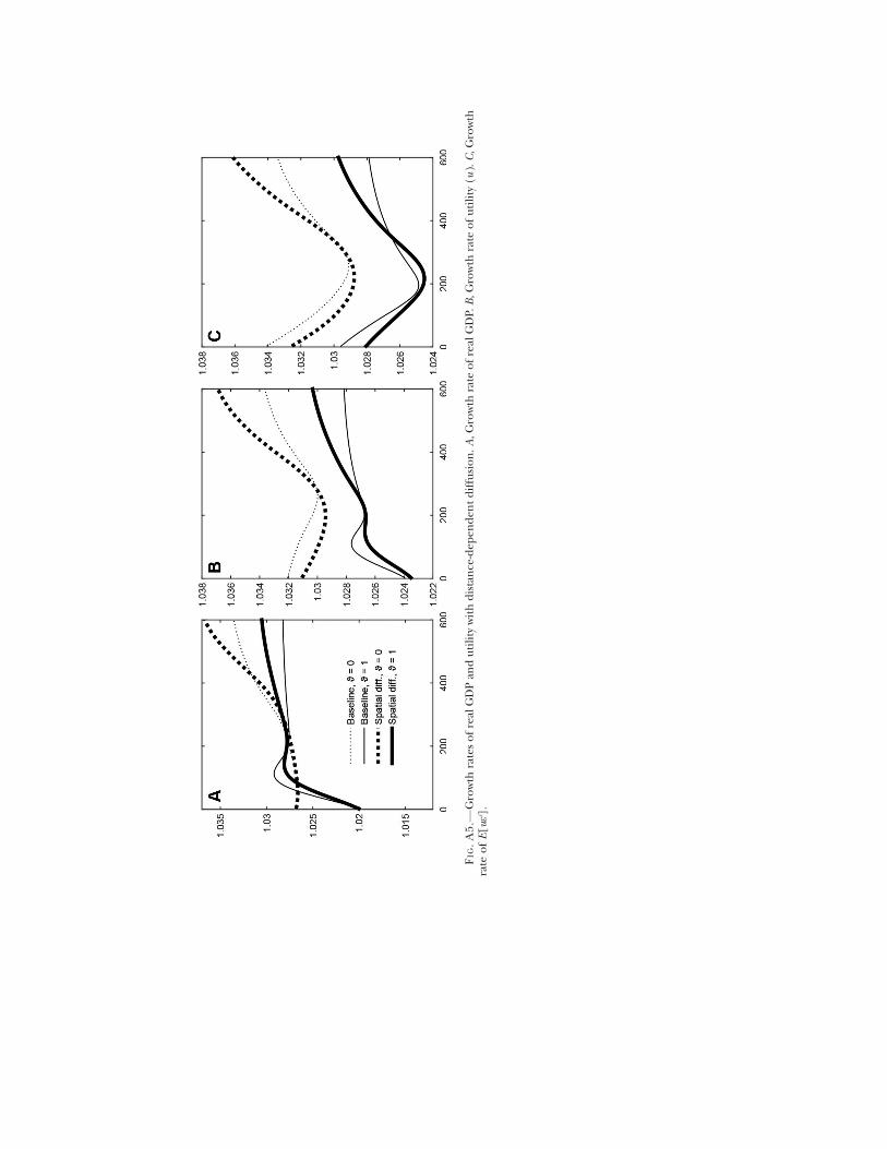
FIG.A5.—

Growth

ratesofreal

GDPan

dutilitywithdistance-dep

enden

tdiffusion.A

,Growth

rate

ofreal

GDP.B,G

rowth

rate

ofutility(u

).C,G

rowth

rate

ofE[uεi].

In terms of the gains from liberalization, the effect on real income increasesfrom 125.8 percent in the benchmark to 131.8 percent in the case with local dif-fusion. Greater movement of people makes it easier for the high-productivityplaces to attract more people, and this is more important when technology ismore concentrated. Focusing on the welfaremeasures yields the opposite results;namely, the gains are smaller than in the benchmark. This result is intuitive: withless diffusion of technology, you get more people living in places they do not par-ticularly like.32

Transportation costs.—As a last robustness check, we increase transportationcosts, first by 20 percent and then by 40 percent. We discuss some of these resultsin the main text. As expected, the rise in transport costs reduces real income andwelfare. Table A4 shows that real output declines by 17.3 percent with an increasein trade costs of 20 percent: a fairly large effect. When transport costs go up by20 percent, the gains from liberalizing migration are higher than in the bench-mark case. The reason is as follows: greater transportation costs increase the in-centives to spatially concentrate. Lower migration costs facilitate this geographicconcentration, hence giving a boost to real income. So trade and migration aresubstitutes. The results are similar, but even larger in magnitude, in the case inwhich transport costs go up by 40 percent.

Appendix B

Proofs, Derivations, and Other Details

A. Derivation of Expected Utility

To determine the expected utility of agents at r, E ½uðr ÞεiðrÞji lives at r �, we firstderive the expected utility of agents who lived at u in period 0 and live at r in pe-riod t.33 The cumulative density function of utility levels ui(u, r) conditional onoriginating from u and choosing to live at r is

32 The PDVs for spatial diffusion are all calculated with a discount factor of b 5 0:9625,since the long-run growth rate exceeds 3.5 percent in the case of no mobility restrictions(and so the PDV would not be well defined with b 5 0:965).

33 Throughout the proof, we omit the time index t for simplicity.


Pr ui u, rð Þ ≤ �ujui u, rð Þ ≥ ui u, sð Þ 8 s ≠ r½ �

5Pr ui u, rð Þ ≤ �u, ui u, rð Þ ≥ ui u, sð Þ 8 s ≠ r½ �

Pr ui u, rð Þ ≥ ui u, sð Þ 8 s ≠ r½ �

5 2

ð�u

0

YSn rf g

e2u sð Þ1=Qm u,sð Þ21=Qz21=Qds 1

Qu rð Þ1=Qm u, rð Þ21=Q

"

� z2 1=Q11ð Þe2u rð Þ1=Qm u,rð Þ21=Qz21=Q

dz

#

� u rð Þ1=Qm u, rð Þ21=Q. ð

S

u sð Þ1=Qm u, sð Þ21=Qds

� �� 5

ð�u

0

21

Q

ðS


� �

� z2 1=Q11ð Þe2

ðS

u sð Þ1=Qm u,sð Þ21=Qds

� �z21=Q

dz

5 e2

ðS

u sð Þ1=Qm u,sð Þ21=Qds

� �z21=Q;

that is, ui(u, r) is distributed Fréchet, and therefore its mean is given by

E ui u, rð Þji originates from u, lives at r½ �

5 G 1 2 Qð ÞðS


� �Q

:

By equation (1), the expected value of u(r)εi(r) equals this expression divided bythe moving costs the agent has to pay,

E u rð Þεi rð Þji originates from u, lives at r½ �

5

G 1 2 Qð ÞðS


� �Q

Qts51m rs21, rsð Þ ,

from which, using assumption 1, we get

E u rð Þεi rð Þji originates from u, lives at r½ �

5 G 1 2 Qð Þm 2 rð ÞðS

u sð Þ1=Qm 2 sð Þ21=Qds

� �Q

;

since this expression does not depend on u, we also have

E u rð Þεi rð Þji lives at r½ � 5 G 1 2 Qð Þm 2 rð ÞðS

u sð Þ1=Qm 2 sð Þ21=Qds

� �Q

,

which is equation (4).

B. Derivation of Trade Shares and the Price Index

We derive here in detail first the probability that a given good produced in anarea r is bought in s. The area B(r, d) (a ball of radius d centered at r) offers dif-


ferent goods in location s. The distribution of prices B(r, d) offered in s is givenby

Gt p, s, B r , dð Þð Þ 5 1 2 e2

ðB r ,dð Þ

Tt rð Þ mct rð Þς s,rð Þp

� 2v

dr

:

The distribution of the prices of the goods s actually buys is then

Gt p, sð Þ 5 1 2 e2

ðS

Tt uð Þ mct uð Þς s,uð Þp

� 2v

du

5 1 2 e2xt sð Þpv

,

where

xt sð Þ 5ðS

Tt uð Þ mct uð Þς s, uð Þ½ �2vdu: (B1)

Now we calculate the probability that a given good produced in an area B(r, d)is bought in s. Start by computing the probability density that the price of thegood produced in B(r, d) and offered in s is equal to p and that this is the lowestprice offered in s. This is

dGt p, s, B r , dð Þð Þdp

e2

ðSnB r ,dð Þ

Tt uð Þ mct uð Þς u,sð Þp

� 2v

du

:

Rewrite

dGt p, s, B r , dð Þð Þ 5 e2

ðB r ,dð Þ

Tt rð Þ mct rð Þς s,rð Þp

� 2v

dr

�ðB r ,dð Þ

Tt rð Þ mct rð Þς r , sð Þ½ �2vdrvpv21dp:

Replace this into the previous expression and integrate over all possible prices,ð∞

0

e2

ðS

Tt uð Þ mct uð Þς s,uð Þp

� 2v

duðB r ,dð Þ

Tt rð Þ mct rð Þς r , sð Þ½ �2vdrvpv21dp:

Solving this integral yields

2e2xt sð Þpv

ðB r ,dð Þ

Tt rð Þ mct rð Þς r , sð Þ½ �2vdr

xt sð Þ

26643775

∞

0

,

which gives

pt s, B r , dð Þð Þ 5

ðB r ,dð Þ

Tt rð Þ mct rð Þς r , sð Þ½ �2vdrðS

Tt uð Þ mct uð Þς u, sð Þ½ �2vdu

5

ðB r ,dð Þ

Tt rð Þ mct rð Þς r , sð Þ½ �2vdr

xt sð Þ


for all r, s ∈ S . Since in any small interval with positive measure there will bemany firms producing many goods, the above expressions can be interpretedas the fraction of goods location s buys from B(r, d). In the limit, as d→ 0, thisexpression can be rewritten as

pt s, rð Þ 5 Tt rð Þ mct rð Þς r , sð Þ½ �2vðS

Tt uð Þ mct uð Þς u, sð Þ½ �2vdu

5Tt rð Þ mct rð Þς r , sð Þ½ �2v

xt sð Þ all r , s ∈ S ,

which is the expression in the text.To finish this subsection, we derive the price index of a location s. We know

that

Pt sð Þ 2r12r 5

ð1

0

pqt sð Þ 2r

12rdq:

This can be interpreted as the average price computed over the different goodsthat are being sold in s. This is the same as the expected value of the price of anygood sold in s, so that

Pt sð Þ 2r12r 5

ð∞

0

p2r12r

dGt sð Þdp

dp:

Since

dGt sð Þdp

5 xt sð Þvpv21e2xt sð Þpv

,

we can write the previous expression as

Pt sð Þ 2r12r 5

ð∞

0

p2r12rxt sð Þvpv21e2xt sð Þpv

dp:

By defining x 5 xtðsÞpv, we can write dx 5 vpv21xtðsÞ. Substituting yieldsð∞

0

x

xt sð Þ� � 2r

12rð Þv

e2xdx,

which is equal to

xt sð Þ r12rð Þv

ð∞

0

x2r12rð Þve2xdx:

The G function is defined as GðaÞ 5 Ð ∞0 y

a21e2ydy, so that we can rewrite the aboveexpression as

xt sð Þ r12rð ÞvG

2r

1 2 rð Þv 1 1

� �:

Therefore,

Pt sð Þ 2r12r 5 xt sð Þ r

12rð ÞvG2r

1 2 rð Þv 1 1

� �,


so that

Pt sð Þ 5 xt sð Þ21v G

2r

1 2 rð Þv 1 1

� �� 212rr

,

which is the expression in the text.

C. Proof of Lemma 2

Substituting (20) and (B1) into (22), we obtain

ut rð Þ 5 �a rð Þ�Lt rð Þ2l y

my 1 g1

wt rð ÞðS

Tt sð Þ mct sð Þς r , sð Þ½ �2vds

� �21v

�p

for any location r, where

�p 5 G2r

1 2 rð Þv 1 1

� �� 212rr

:

We can rewrite this as

�a rð Þ2vwt rð Þ2v�Lt rð Þlv 5 my 1 g1

y

� �2v

ut rð Þ�pð Þ2v

ðS

Tt sð Þ½mct sð Þς r , sð Þ�2vds,

from which


� �2v

wt rð Þ2v�Lt rð Þlv

5 k1

ðS

tt sð Þς r , sð Þ2vwt sð Þ2v�Lt sð Þa2 12m2g1yð Þvds,

(B2)

where

k1 5my 1 g1

y

� �2 m1g1y½ �vmmv yn

g1

� �2g1vy

�p2v:

This yields the first set of equations that ut(⋅), �Ltð⋅Þ, and wt(⋅) have to solve.Inserting (19) and (20) into the balanced trade condition, we get

wt rð ÞH rð Þ�Lt rð Þ 5 �p2v

ðS

Tt rð Þ mct rð Þς r , sð Þ½ �2vPt sð Þvwt sð ÞH sð Þ�Lt sð Þds:

Substituting (22) and Ttðr Þ 5 ttðr Þ�Ltðr Þa into the previous equation yields

tt rð Þ21H rð Þwt rð Þ11v�Lt rð Þ12a1 12m2g1yð Þv

5 k1

ðS


� �v

H sð Þς s, rð Þ2vwt sð Þ11v�Lt sð Þ12lvds:(B3)

This gives the second set of equations that ut(⋅), �Ltð⋅Þ, and wt(⋅) have to solve. Thethird set of equations that ut(⋅), �Ltð⋅Þ, and wt(⋅) have to solve is given by (7). Clearly,tt(⋅) is obtained directly from (8) and �Lt21ð⋅Þ.


We can use (B2) and (B3) to analyze the equilibrium allocation further undersymmetric trade costs. In doing so, we follow the proof of theorem 2 in Allen andArkolakis (2014). Assume trade costs are symmetric so that ςðr , sÞ 5 ςðs, r Þ. Intro-duce the following function, which is the ratio of the left-hand sides of (B1) and(B2):

f1 rð Þ 5 tt rð Þ21H rð Þwt rð Þ11v�Lt rð Þ12a1 12m2g1yð Þv

�a rð Þut rð Þh i2v

wt rð Þ2v�Lt rð Þlv:

Obviously, f1(r) equals the ratio of the right-hand sides, that is,

f1 rð Þ 5

ðS

�a sð Þut sð Þh iv

H sð Þwt sð Þ11v�Lt sð Þ12lvς s, rð Þ2vdsðS

tt sð Þwt sð Þ2v�Lt sð Þa2 12m2g1yð Þvς r , sð Þ2vds

,

from which, using ςðr , sÞ 5 ςðs, r Þ, we obtain

f1 rð Þ 5

ðS

f1 sð Þ2lf2 s, rð ÞdsðS

f1 sð Þ2 11lð Þf2 s, rð Þds, (B4)

where

f2 s, rð Þ 5 tt sð Þ2l

ς s, rð Þv�a sð Þut sð Þ

� � 11lð ÞvH sð Þ11lwt sð Þ11v1 112vð Þl

� �Lt sð Þ12lv2l a211 l1g1y2 12mð Þ½ �v½ �:

Write (B4) as

f3 rð Þ 5 f1 rð Þ2lðS

f1 sð Þ2lf2 s, rð Þds5

f1 rð Þ2 11lð ÞðS

f1 sð Þ2 11lð Þf2 s, rð Þds: (B5)

Then, using the notation

g1 rð Þ 5 f1 rð Þ2l

and

g2 rð Þ 5 f1 rð Þ2 11lð Þ,

one can write this last equation as

g1 rð Þ 5ðS

f3 rð Þf2 s, rð Þg1 sð Þds (B6)

and

g2 rð Þ 5ðS

f3 rð Þf2 s, rð Þg2 sð Þds: (B7)


Define K(s, r) as the value of f3(r)f2(s, r) evaluated at the solution g1. By (B5),the value of f3(r)f2(s, r) evaluated at g2 is the same for any pair of locations (r, s).Therefore, g1 and g2 are both solutions to the integral equation

x rð Þ 5ðS

K s, rð Þx sð Þds: (B8)

Note that K(s, r) is nonnegative, continuous, and square-integrable. Nonnega-tivity of K(⋅, ⋅) immediately follows from the nonnegativity of f2 and f3. To seemea-surability, recall that �aðr Þ,H(r), and t0(r) are assumed to be continuous functions.We also need to assume that u0(r),w0(r), and �L0ðr Þ are continuous; otherwise, theintegrals on the right-hand sides of (B2) and (B3) would not be well defined.Once this is the case, t1(r) is also continuous by (8); hence so are u1(r), w1(r),and �L1ðr Þ. Using this logic, one can show that t1(r), ut(r), wt(r), and �Ltðr Þ are con-tinuous for any t. Thus, f1, f2, and f3 are all continuous, which implies that K(⋅, ⋅) iscontinuous.34 Square-integrability, which meansð

S

ðS

K s, rð Þ2dsdr < ∞,

is due to the fact that S is boundedby assumption, but so isK(⋅, ⋅). To seewhyK(⋅, ⋅)is bounded, note that population at a location cannot shrink to zero unless thelocation offers zero nominal wages that compensate for its infinitely good ameni-ties. Also, population at a location cannot be larger than �L. These upper and lowerbounds on population translate into upper and lower bounds on f2(⋅, ⋅) and f3(⋅)and hence on K(⋅, ⋅).

Given the above properties of K(⋅, ⋅), theorem 2.1 in Zabreyko et al. (1975)guarantees that the solution to (B8) exists and is unique up to a scalar multiple.Hence

g1 rð Þ 5 -g2 rð Þ,where ϖ is a constant. Therefore, we have

f1 rð Þ2l 5 -f1 rð Þ2 11lð Þ,

from which

f1 rð Þ 5 -:

That is,

tt rð Þ21H rð Þwt rð Þ11v�Lt rð Þ12a1 12m2g1yð Þv

�a rð Þut rð Þh i2v

wt rð Þ2v�Lt rð Þlv5 -;

thus

34 A rigorous proof of the measurability of K(⋅, ⋅) requires some further steps that wehave not included in this draft but are available on request. We acknowledge the help ofÁron Tóbiás in formulating this more rigorous proof.


wt rð Þ 5 -1

112v�a rð Þut rð Þ

� �2 v112v

tt rð Þ 1112vH rð Þ2 1

112v�Lt rð Þa211 l1

g1y2 12mð Þ½ �v

112v ,

which is the same as equation (23), with �w defined as �w 5 -1=ð112vÞ.Substituting this into (B2) yields the second equation in lemma 2:


� �2v 11vð Þ112v

tt rð Þ2 v112vH rð Þ v

112v�Lt rð Þlv2 v112v a211 l1g1

y2 12mð Þ½ �v½ �

5 k1

ðS


� � v2

112v

tt sð Þ 11v112vH sð Þ v

112vς r , sð Þ2v

� �Lt sð Þ12lv1 11v112v a211 l1g1

y2 12mð Þ½ �v½ �ds:

(B9)

QED

D. Proof of Lemma 3

Substituting (7) in (24) yields

B1t rð Þut rð Þ1Qlv2 v

112v a211 l1g1y2 12m½ �½ �v½ �½ �1v 11vð Þ

112v

5 k1

ðS

ut sð Þ1Q12lv1 11v

112v a211 l1g1y2 12m½ �½ �v½ �½ �2 v2

112vB2t sð Þς r , sð Þ2vds,(B10)

where

B1t rð Þ 5 �a rð Þ2v 11vð Þ112v tt rð Þ2 v

112vH rð Þ v112v a1 l1g1

y2 12m½ �½ �v½ �2lv

�m2 rð Þ21Qlv2 v

112v a211 l1g1y2 12m½ �½ �v½ �½ �

and

B2t r , sð Þ 5 �a sð Þ v2

112vtt sð Þ 11v112vH sð Þ v

112v211lv2 11v112v a211 l1g1

y2 12m½ �½ �v½ �

�m 2 sð Þ21Q12lv1 11v

112v a211 l1g1y2 12m½ �½ �v½ �½ �ς r , sð Þ2v

are exogenously given functions, and

ut rð Þ 5 ut rð Þ�Lð

S

ut vð Þ1=Qm2 vð Þ21=Qdv

26643775

Q 12 v1Q

l1 12mð Þ2g1y½ �v2a½ �1v

� �: (B11)

First we prove that a solution to (B10) exists and is unique if a=v 1 g1=y ≤ Q 1l 1 1 2 m. Equations (B10) constitute a system of equations that pin down utðr Þ.It follows from theorem 2.19 in Zabreyko et al. (1975) that the solution f(⋅) toequation

B1 rð Þf rð Þ~g1 5 k1

ðS

B2 r , sð Þf sð Þ~g2ds


exists and is unique if (i) the function k1B1ðrÞ21B2ðr , sÞ is strictly positive and con-tinuous, which is a direct consequence of assumption 3, and (ii) j~g2=~g1j ≤ 1; thatis, the ratio of exponents on the right-hand side and on the left-hand side is notlarger than one in absolute value. In the case of equation (B10), this conditionimplies

1Q

1 2 lv 1 11v112v a 2 1 1 l 1 g1

y2 1 2 m½ �

h iv

h ih i2 v2

112v

1Q

lv 2 v112v a 2 1 1 l 1 g1

y2 1 2 m½ �

h iv

h ih i1 v 11vð Þ

112v

≤ 1,

from which, by arranging, we get

a

v1

g1

y≤ l 1 1 2 m 1 Q:

Theorem 2.19 in Zabreyko et al. (1975) also implies that we can solve equation(B10) using the following iterative procedure. Guess an initial distribution, u0

t ð⋅Þ.Plug it into the right-hand side of equation (B10), calculate the left-hand side,and solve for the distribution of utility; call this u1

t ð⋅Þ. Then compute the distancebetween u1

t ð⋅Þ and u0t ð⋅Þ, defined as

dist1t 5

ðS

u1t rð Þ 2 u0

t rð Þ� 2dr :

If dist1t < ε, where ε is an exogenously given tolerance level, stop. Otherwise, plugu1t ð⋅Þ into the right-hand side of (B10), obtain the updated distribution u2

t ðr Þ, andcompute dist2t , defined analogously to dist1t . Continue the procedure until dist

it <

ε for some i.To obtain ut(⋅) from utð⋅Þ, we write equation (B11) as

ut rð Þ 5 ut rð ÞU Ϝ

t

, (B12)

where

Ut 5�Lð

S

m2 vð Þ21=Qut vð Þ1=Qdv(B13)

is independent of r and

ϜQ5 1 2

v

1Q

l 1 1 2 mð Þ 2 g1

y

h iv 2 a

h i1 v

:

Plugging (B12) into (B13) and rearranging yields

U12Ϝ

Qt 5

�LðS

m2 vð Þ21=Qut vð Þ1=Qdv:

Therefore, the value of Ut can be uniquely expressed as


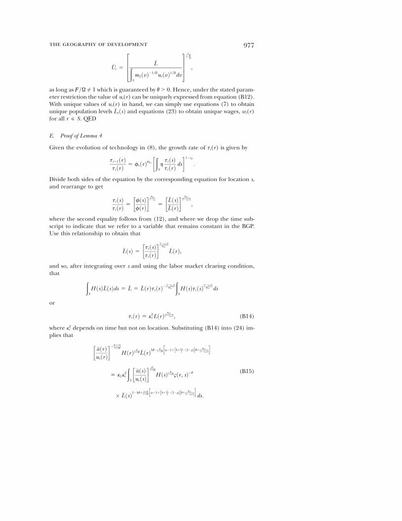
Ut 5�Lð

S

m2 vð Þ21=Qut vð Þ1=Qdv

26643775

112Ϝ

Q

,

as long as Ϝ=Q ≠ 1 which is guaranteed by v > 0. Hence, under the stated param-eter restriction the value of ut(r) can be uniquely expressed from equation (B12).With unique values of ut(r) in hand, we can simply use equations (7) to obtainunique population levels �LtðsÞ and equations (23) to obtain unique wages, wt(r)for all r ∈ S . QED

E. Proof of Lemma 4

Given the evolution of technology in (8), the growth rate of tt(r) is given by

tt11 rð Þtt rð Þ 5 ft rð Þvg1

ðS


� �12g2

:

Divide both sides of the equation by the corresponding equation for location s,and rearrange to get

tt sð Þtt rð Þ 5

f sð Þf rð Þ

� � vg112g2

5�L sð Þ�L rð Þ

� � vg112g2ð Þy

,

where the second equality follows from (12), and where we drop the time sub-script to indicate that we refer to a variable that remains constant in the BGP.Use this relationship to obtain that

�L sð Þ 5 tt sð Þtt rð Þ

� � 12g2ð Þyvg1

�L rð Þ,

and so, after integrating over s and using the labor market clearing condition,that ð

S

H sð Þ�L sð Þds 5 �L 5 �L rð Þtt rð Þ2 12g2ð Þyvg1

ðS

H sð Þtt sð Þ 12g2ð Þyvg1 ds

or

tt rð Þ 5 k2t L rð Þ vg112g2ð Þy, (B14)

where k2t depends on time but not on location. Substituting (B14) into (24) im-plies that


� �2v 11vð Þ112v

H rð Þ v112v�L rð Þlv2 v

112v a211 l1g1y2 12m½ �½ �v1 vg1

12g2ð Þy

h i

5 k1k2t

ðS


� � v2

112v

H sð Þ v112vς r , sð Þ2v

� �L sð Þ12lv1 11v112v a211 l1g1

y2 12m½ �½ �v1 vg1

12g2ð Þy

h ids:

(B15)


Substituting equation (7) in (B15) yields


� �2v 11vð Þ112v

H rð Þ v112v



�L

H rð Þ

26643775

lv2 v112v a211 l1g1

y2 12m½ �½ �v1 vg1

12g2ð Þy

h i

5 k1k2t

ðS


� � v2

112v

H sð Þ v112vς r , sð Þ2v

� ut sð Þ1=Qm 2 sð Þ21=QðS


�L

H sð Þ

26643775

12lv1 11v112v a211 l1g1

y2 12m½ �½ �v1 vg1

12g2ð Þy

h ids,

(B16)

where time subscripts have been dropped for variables that do not change in theBGP. Rearranging (B16) yields

B1 rð Þut rð Þ1Q

lv2 v112v a211 l1g1

y2 12m½ �½ �v1 vg1

12g2ð Þy

h ih i1v 11vð Þ

112v

5 k1k2t

ðS

ut sð Þ1Q

12lv1 11v112v a211 l1g1

y2 12m½ �½ �v1 vg1

12g2ð Þy

h ih i2 v2

112vB2 sð Þς r , sð Þ2vds,

(B17)

where

B1 rð Þ 5 �a rð Þ2v 11vð Þ112v H rð Þ v

112v a1 l1g1y2 12m½ �½ �v1 vg1

12g2ð Þy

h i2lv

�m 2 rð Þ21Q

lv2 v112v a211 l1g1

y2 12m½ �½ �v1 vg1

12g2ð Þy

h ih iand

B2 sð Þ 5 �a sð Þ v2

112vH sð Þ v112v211lv2 11v

112v a211 l1g1y2 12m½ �½ �v1 vg1

12g2ð Þy

h i

�m 2 sð Þ21Q

12lv1 11v112v a211 l1g1

y2 12m½ �½ �v1 vg1

12g2ð Þy

h ih iare exogenously given functions, and

ut rð Þ 5 ut rð Þ ~Ut , (B18)

where

~Ut 5�Lð

S


26643775

Q 12 v

1Q

l1 12mð Þ2g1y½ �v2a2

vg112g2ð Þy

h i1v

24 35:

Equations (B17) constitute a system of equations that pin down utðr Þ. It followsfrom theorem 2.19 in Zabreyko et al. (1975) that the solution f(⋅) to equation


B1 rð Þf rð Þ~g1 5 B3

ðS

B2 sð Þf sð Þ~g2ds

exists and is unique if j~g2=~g1j ≤ 1; that is, the ratio of exponents on the right-hand side and on the left-hand side is not larger than one in absolute value.In the case of equation (B17), this condition implies

1Q

1 2 lv 1 11v112v a 2 1 1 l 1 g1

y2 1 2 m½ �

h iv 1 vg1

12g2ð Þyh ih i

2 v2

112v

1Q

lv 2 v112v a 2 1 1 l 1 g1

y2 1 2 m½ �

h iv 1 vg1

12g2ð Þyh ih i

1 v 11vð Þ112v

≤ 1,

from which, by arranging, we get

a

v1

g1

y1

g1

1 2 g2ð Þy ≤ l 1 1 2 m 1 Q:

Once we have found a solution utðr Þ, the rest of the equilibrium calculation pro-ceeds as in lemma 3. QED

F. Proof of Lemma 5

Lemma 4 guarantees that if the economy is in its BGP in periods t and t1 1, then


k2t11

k2t

� �1v

5tt11 rð Þtt rð Þ

� �1v

for all r; so since

tt11 rð Þtt rð Þ 5 f rð Þvg1

ðS


� �12g2

5 f rð Þvg1

ðS

hf sð Þf rð Þ

� � vg112g2

ds

" #12g2

5 h12g2g1=n

g1 1 my

� �vg1yðS

�L sð Þ vg112g2½ �yds

� �12g2

,

we have that

ut11 rð Þut rð Þ 5 h

12g2v

g1=n

g1 1 my

� �g1yðS

�L sð Þ vg112g2½ �yds

� �12g2v

:

QED

G. Procedure to Find a Solution to Equation (32)

We use the following procedure to solve equation (32). We approximate (32) by

w0 rð Þ2v�L0 rð Þlv �a rð Þu0 rð Þ

� �2v

5 k1�w2 112v½ �

ðS

w0 sð Þ11v�L0 sð Þ12lvH sð Þς r , sð Þ2v �a sð Þu0 sð Þ

� �v2e0

ds,

(B19)


where e0 > 0 is a constant. For any positive e0, theorem 2.19 in Zabreyko et al.(1975) guarantees that (B19) can be solved by the following simple iterative pro-cedure. Guess some initial distribution ½�aðr Þ=u0ðr Þ�0e0 , plug it into the right-handside of equation (B19), calculate the left-hand side, and solve for �aðr Þ=u 0ðrÞ; callthis ½�aðr Þ=u0ðr Þ�1e0 . Compute the distance between ½�aðrÞ=u0ðr Þ�1e0 and ½�aðrÞ=u0ðr Þ�0e0 ,defined as

dist1 5

ðS

�a rð Þu 0 rð Þ

� �1

e02

�a rð Þu 0 rð Þ

� �0

e0

� �2

dr :

If dist1 < ε, where ε is an exogenously given tolerance level, stop. Otherwise, plug½�aðr Þ=u 0ðr Þ�1e0 into the right-hand side of (B19), express �aðr Þ=u 0ðr Þ from the left-hand side, that is, obtain ½�aðr Þ=u0ðrÞ�2e0 , and compute dist2, defined analogouslyto dist1. Continue the procedure until disti < ε for some i.

Having the solution to (B19), ½�aðrÞ=u0ðrÞ�e0 , one needs to check whether it issufficiently close to the solution of (32). Given that the system of (24) and (23)is equivalent to the system of (32) and (31), we can check this in the followingway. First, we solve for t0ðr Þe0 using ½�aðr Þ=u0ðr Þ�e0 and equation (31). Next, we plug½�aðr Þ=u0ðr Þ�e0 and t0ðrÞe0 into (24) and solve for population levels �Lðr Þe0 .35 Finally,we check whether �L 0ðr Þe0 are sufficiently close to �L 0ðrÞ, the population levels seenin the data.36 If they are not close enough, we take e1 5 e0=2 and redo the wholeprocedure with e1 instead of e0. Now, if �L 0ðrÞe1 are sufficiently close to �L 0ðr Þ, westop. Otherwise, we proceed with e2 5 e1=2; and so on. This procedure resultsin a pair of distributions ½�aðr Þ=u 0ðr Þ�ei and t0ðr Þei , which are sufficiently close tothe solution of (32) and (31).

Appendix C

Data Appendix

The data description and sources follow approximately the order in which theyappear in the paper. For the numerical exercise, all data are essentially for thetime period 2000–2010, whereas for the calibration of the parameters we some-times use data from a longer time period.

Population and amenities of US metropolitan statistical areas.—Data on populationof USMSAs come from the Bureau of Economic Analysis, Regional Economic Ac-counts, and are for the years 2005 and 2008. Corresponding data on amenities areestimated by the structural model in Desmet and Rossi-Hansberg (2013).

Population, GDP, and wages at 17 � 17 resolution.—Data on population and GDPfor 17� 17 cells for the entire world come from the G-Econ 4.0 research project atYale University. For the calibration of the technology parameters, we use data of

35 This is done using the procedure explained in Sec. IV.F.36 The criterion used here is

gdist0 5 ðS

�L 0 rð Þe0 2 �L 0 rð Þ½ �2dr < ~ε,

where ~ε is a positive tolerance level.


1990, 1995, 2000, and 2005 and take GDP measured in purchasing power parity(PPP) terms. For the benchmark model, we use data of 2000. Wages are taken tobe GDP in PPP terms divided by population.

Railroads, major roads, other roads, and waterways at 17 � 17 resolution.—Data onrailroads, major roads, and other roads come from http://www.naturalearthdata.com/, a public-domainmap data set built through the collaborative effort of manyvolunteers and supported by the North American Cartographic Information Soci-ety. For each 17� 17 cell, we define railroads as the share of 0.17� 0.17 cells throughwhich a railroad passes. Major roads, other roads, and waterways are defined anal-ogously. Major roads refer to a major highway, a beltway, or a bypass; other roadsrefer to any other type of road; and waterways refer to either a river or an ocean.

Land at 17 � 17 and 30 00 � 30 00 resolution.—Data on land come from the GlobalLand One-km Base Elevation (GLOBE) digital elevation model (DEM), a rasterelevation data set from the National Oceanic and Atmospheric Administrationcovering all 3000 � 3000 (arcsecond) cells that are located on land. Using this infor-mation, we compute for each 17 � 17 cell on the globe the share of the 3000 � 3000

cells that are on land.Subjective well-being at country level.—Subjective well-being is measured on a

Cantril ladder from 0 to 10, where 0 represents the worst possible life and 10 thebest possible life the individual can contemplate for himself. The main datasource is the Gallup World Poll, and we take the mean for the period 2007–11as reported in the Human Development Report 2013. This gives us data on 151countries. To increase the coverage of countries, we proceed in three ways. First,we use the 2013 World Database of Happiness by R. Veenhoven (http://worlddatabaseofhappiness.eur.nl), who reports data for a similar time period on thesame evaluative measure of subjective well-being from Gallup, the Pew ResearchCenter, and Latinobarómetro. This gives an additional seven countries. Second,Abdallah, Thompson, and Marks (2008) propose a model to estimate subjectivemeasures of well-being for countries that are typically not surveyed. To make thedata comparable, we normalize the Abdallah et al. measure so that the countriesthat are common with those surveyed by Gallup have the same means and stan-dard deviations. This increases the coverage to 184 countries. Third, for the restof the world—mostly small islands and territories—we assign subjective well-beingmeasures in an ad hoc manner. For example, for Andorra we take the average ofFrance and Spain. For another example, in the case of Nauru, a small island inthe Pacific, we take the average of the Solomon Islands and Vanuatu.

Population at 30 00 � 30 00 resolution.—Population data at the same resolution of3000 � 3000 come from LandScan 2005 at the Oak Ridge National Laboratory.

US zip code and CBSA data.—Data on area, population, mean earnings perworker, and income per capita come from the US census. Data referred to as2000 are from the 2000 census, and data referred to as 2007–11 come from the2007–11 American Community Survey 5-year estimates. The geographic unit ofobservation is the ZIP Code Tabulation Areas (ZCTAs).

Data on payroll and number of employees for US zip codes in 2010 come fromthe ZIP Code Business Patterns from the US Census Bureau. Note that zip codesand ZCTAs are not exactly the same. In particular, zip codes do not have areas.ZCTAs should be understood as areal representations of US Postal Service zipcodes. When calculating employee density for zip codes, we therefore use the


corresponding ZCTAs. Tomatch ZCTAs to CBSA, we rely on tabulation files fromthe US Census Bureau.

Historical population data.—Country-level historical population data for the pe-riod 1950–2000 come from the Penn World Tables 8.1. Similar data for 1920 and1870 come from Maddison (2001).

References

Abdallah, S., S. Thompson, and N. Marks. 2008. “Estimating Worldwide Life Sat-isfaction.” Ecological Econ. 65 (1): 35–47.

Albouy, D., W. Graf, R. Kellogg, and H. Wolff. 2016. “Climate Amenities, ClimateChange, and American Quality of Life.” J. Assoc. Environmental and ResourceEcon. 3 (1): 205–46.

Allen, T., and C. Arkolakis. 2014. “Trade and the Topography of the Spatial Econ-omy.” Q.J.E. 129 (3): 1085–1140.

Behrens, K., G. Mion, Y. Murata, and J. Suedekum. 2017. “Spatial Frictions.”J. Urban Econ. 97 (C): 40–70.

Bernard, A. B., J. Eaton, J. B. Jensen, and S. Kortum. 2003. “Plants and Produc-tivity in International Trade.” A.E.R. 93 (4): 1268–90.

Caliendo, L., F. Parro, E. Rossi-Hansberg, and P. Sarte. 2018. “The Impact of Re-gional and Sectoral Productivity Changes in the U.S. Economy.” Rev. Econ.Studies, forthcoming.

Carlino, G., S. Chatterjee, and R. Hunt. 2007. “Urban Density and the Rate ofInvention.” J. Urban Econ. 61:389–419.

Combes, P., G. Duranton, L. Gobillon, D. Puga, and S. Roux. 2012. “The Produc-tivity Advantages of Large Cities: Distinguishing Agglomeration from Firm Se-lection.” Econometrica 80:2543–94.

Comin, D. A., M. Dmitriev, and E. Rossi-Hansberg. 2012. “The Spatial Diffusionof Technology.” Working Paper no. 18534, NBER, Cambridge, MA.

Costinot, A., and A. Rodríguez-Clare. 2014. “Trade Theory with Numbers: Quan-tifying the Consequences of Globalization.” In Handbook of International Eco-nomics, vol. 4, edited by Gita Gopinath, Elhanan Helpman, and Kenneth Ro-goff, 197–261. Amsterdam: Elsevier.

Davis, M. A., and F. Ortalo-Magné. 2011. “Household Expenditures, Wages,Rents.” Rev. Econ. Dynamics 14 (2): 248–61.

Deaton, A. 2008. “Income, Health, and Well-Being around the World: Evidencefrom the Gallup World Poll.” J. Econ. Perspectives 22 (2): 53–72.

Deaton, A., and A. Stone. 2013. “TwoHappiness Puzzles.” A.E.R. 103 (3): 591–97.Desmet, K., and J. Rappaport. 2017. “The Settlement of the United States, 1800–

2000: The Long Transition towards Gibrat’s Law.” J. Urban Econ. 98 (March):50–68.

Desmet, K., andE. Rossi-Hansberg. 2013. “UrbanAccounting andWelfare.”A.E.R.103 (6): 2296–2327.

———. 2014. “Spatial Development.” A.E.R. 104 (4): 1211–43.———. 2015. “On the Spatial Economic Impact of Global Warming.” J. Urban

Econ. 88:16–37.Diamond, R. 2016. “The Determinants and Welfare Implications of US Workers’

Diverging Location Choices by Skill: 1980–2000.” A.E.R. 106 (3): 479–524.Eaton, J., and S. Kortum. 2002. “Technology, Geography, and Trade.” Econometrica

70 (5): 1741–79.


Fajgelbaum, P., E. Morales, J. Suarez Serrato, and O. Zidar. 2016. “State Taxesand Spatial Misallocation.” Manuscript, Princeton Univ.

Fajgelbaum, P., and S. Redding. 2014. “External Integration, Structural Transfor-mation and Economic Development: Evidence from Argentina 1870–1914.”Manuscript, Princeton Univ.

Glaeser, E. L., J. D. Gottlieb, and O. Ziv. 2016. “Unhappy Cities.” J. Labor Econ. 34(S2): S129–S182.

Greenwood, J., Z. Hercowitz, and P. Krusell. 1997. “Long-Run Implications ofInvestment-Specific Technological Change.” A.E.R. 87 (3): 342–62.

Head, K., and T. Mayer. 2014. “Gravity Equations: Workhorse, Toolkit, and Cook-book.” In Handbook of International Economics, vol. 4, edited by Gita Gopinath,Elhanan Helpman, and Kenneth Rogoff, 131–95. Amsterdam: Elsevier.

Jones, C. I. 1995. “R&D-Based Models of Economic Growth.” J.P.E. 103 (4): 759–84.

Kahneman, D., and A. Deaton. 2010. “High Income Improves Evaluation of Lifebut Not Emotional Well-Being.” Proc. Nat. Acad. Sci. 107 (38): 16489–93.

Kennan, J. 2013. “Open Borders.” Rev. Econ. Dynamics 16 (2): L1–L13.Klein, P., and G. Ventura. 2007. “TFP Differences and the Aggregate Effects of

Labor Mobility in the Long Run.” B.E. J. Macroeconomics 7 (1): 1–36.Kline, P., and E. Moretti. 2014. “Local Economic Development, Agglomeration

Economies, and the Big Push: 100 Years of Evidence from the Tennessee Val-ley Authority.” Q.J.E. 129 (1): 275–331.

Maddison, A. 2001.TheWorld Economy: AMillennial Perspective. Paris: DevelopmentCentre of the OECD.

Monte, F., S. Redding, and E. Rossi-Hansberg. 2018. “Commuting, Migration andLocal Employment Elasticities.” A.E.R., forthcoming.

Ortega, F., and G. Peri. 2013. “The Effect of Income and Immigration Policies onInternational Migration.” Migration Studies 1 (1): 47–74.

Roback, J. 1982. “Wages, Rents, and the Quality of Life.” J.P.E. 90 (6): 1257–78.Rosen, S. 1979. “Wage-Based Indexes of Urban Quality of Life.” In Current Issues

in Urban Economics, edited by Peter M. Mieszowski and Mahlon R. Straszheim,74–104. Baltimore: Johns Hopkins Univ. Press.

Simonovska, I., and W. E. Waugh. 2014. “Trade Models, Trade Elasticities, andthe Gains from Trade.” Working Paper no. 20495, NBER, Cambridge, MA.

Stevenson, B., and J. Wolfers. 2013. “Subjective Well-Being and Income: Is ThereAny Evidence of Satiation?” A.E.R. 103 (3): 598–604.

Zabreyko, P., A. Koshelev, M. Krasnoselskii, S. Mikhlin, L. Rakovshchik, and V.Stet’senko. 1975. Integral Equations: A Reference Text. Leyden: Noordhoff.


the geography of development - princeton universityerossi/gd.pdf · to the data for the whole world...

Documents