The general inefficiency of batch training for gradient

descent learning

D. Randall Wilsona,*, Tony R. Martinezb,1

aFonix Corporation, 180 West Election Road Suite 200, Draper, UT, USAbComputer Science Department, 3361 TMCB, Brigham Young University, Provo, UT 84602, USA

Received 10 July 2001; revised 8 April 2003; accepted 8 April 2003

Abstract

Gradient descent training of neural networks can be done in either a batch or on-line manner. A widely held myth in the neural network

community is that batch training is as fast or faster and/or more ‘correct’ than on-line training because it supposedly uses a better

approximation of the true gradient for its weight updates. This paper explains why batch training is almost always slower than on-line

training—often orders of magnitude slower—especially on large training sets. The main reason is due to the ability of on-line training to

follow curves in the error surface throughout each epoch, which allows it to safely use a larger learning rate and thus converge with less

iterations through the training data. Empirical results on a large (20,000-instance) speech recognition task and on 26 other learning tasks

demonstrate that convergence can be reached significantly faster using on-line training than batch training, with no apparent difference in

accuracy.

q 2003 Elsevier Ltd. All rights reserved.

Keywords: Batch training; On-line training; Gradient descent; Backpropagation; Learning rate; Optimization; Stochastic approximation; Generalization

1. Introduction

Neural networks are often trained using algorithms that

approximate gradient descent. Gradient descent learning

(also called steepest descent) can be done using either a

batch method or an on-line method. In batch training,

weight changes are accumulated over an entire presentation

of the training data (an epoch) before being applied, while

on-line training updates weights after the presentation of

each training example (instance). Another alternative is

sometimes called mini-batch (Sarle, 2002), in which weight

changes are accumulated over some number u of instances

before actually updating the weights. Using an update

frequency (or batch size) of u ¼ 1 results in on-line training,

while u ¼ N results in batch training, where N is the number

of instances in the training set. In each case a learning rate,

r; is used to adjust the size of weight changes.

Most neural network researchers would agree that the

question of whether batch or on-line training is faster and/or

‘better’ has been settled. However, it is interesting to note

that people have unknowingly ‘settled’ upon two opposing

views. Some believe that since batch uses the ‘true’ gradient

direction for its updates, it is more ‘correct,’ and some

researchers claim or imply that batch training is faster.

Others note that in practice on-line training appears to train

more quickly and produce better results than batch training.

This paper explains why on-line training can be expected

to be at least as accurate as well as faster than batch training,

and demonstrates empirically that on-line training is often

orders of magnitude faster than batch training, especially on

large training sets.

To briefly overview the main points of this paper, batch

training is able to calculate the direction of the true gradient,

but it does not know how far it can safely go in that direction

before the gradient changes direction (or begins to go back

‘uphill’). The true gradient can curve considerably on its

way to a minimum, but batch training can only take one step

for each epoch, and each step is in a straight line.

As the size of the training set grows, the accumulated

weight changes for batch training become large. This leads

batch training to use unreasonably large steps, which in turn

leads to unstable learning and to the overshooting of curves

0893-6080/$ - see front matter q 2003 Elsevier Ltd. All rights reserved.

doi:10.1016/S0893-6080(03)00138-2

Neural Networks 16 (2003) 1429–1451

www.elsevier.com/locate/neunet

1 Tel.: þ1-801-422-6464; fax: þ1-801-422-7775.

* Corresponding author. Tel.: þ1-801-446-1697.

E-mail address: randy@axon.cs.byu.edu (D.R. Wilson).

and local minima in the error landscape. Therefore, a

reduction in the size of the learning rate (or, equivalently,

using the average weight change instead of the sum) is

required for batch training to be stable as the size of the

training set grows. However, this means that the larger the

training set is, the more computation is required for a weight

change of the same magnitude.

On the other hand, on-line training uses the ‘local’

gradient of each training instance to determine what

direction to go. These local gradients can be noisy and

contradict each other, but will on average move in the

direction of the true gradient. Since on-line training updates

weights after each instance, it is able to follow curves in the

gradient during the course of an epoch. It can also handle

any size of training set without having to reduce the learning

rate.

Section 2 surveys the neural network literature to

examine what is currently being taught about on-line and

batch training. Some of the references make false claims or

use misleading examples, while others appear entirely

accurate. None of the literature surveyed, however, men-

tions the ability of on-line training to learn faster as a result

of being able to follow the gradient more closely during an

epoch and thus use a larger learning rate.

Section 3 explains the above arguments in more detail,

describes each training method in terms of optimization

theory, and gives several intuitive interpretations of batch

and on-line training. It discusses how on-line and batch are

similar in order to focus in on what is really different

between the methods and how this difference gives on-line

training such an advantage.

Some readers may find that Section 3 contains a bit of

redundancy, in terms of explaining the same thing in several

different ways. However, it is the experience of the authors

that some neural network researchers have a difficult time

overcoming long-held misunderstandings in this area (while

others understand quickly and wonder what all the

confusion is about). Hopefully by presenting the arguments

in several ways there will remain little room for

misunderstanding.

Section 4 presents empirical results of training multilayer

perceptrons using error backpropagation with a variety of

learning rates on 26 classification tasks from the UCI

Machine Learning Database Repository (Blake & Merz,

1998), with both on-line and batch training. It also compares

on-line, batch and mini-batch training on a speech

recognition task with a large training set of 20,000

instances. The results strongly support the claim that on-

line training is faster and at least as accurate as batch

training, especially for large training sets. The speech

recognition experiments also show that the larger the batch

size is, the more on-line training outperforms batch training.

Section 4 also explains why using clusters of machines

training a single neural network in parallel—which requires

batch or mini-batch training—is likely to be slower (as well

as more expensive) than using on-line training on a single

machine to do the training alone.

Section 5 summarizes the conclusions from these results,

which basically are that there are strong disadvantages and

no apparent real advantages to using batch training, even for

parallel training, and that on-line training should therefore

be used in practical gradient descent training situations.

2. Survey of neural network literature

This section surveys the neural network literature to

examine what is currently being taught about on-line and

batch training. As evidenced from the literature and from

recent discussions with various researchers, many are still of

the opinion that batch training is as fast or faster and/or more

correct than on-line training. Unfortunately, this belief may

lead those who use gradient descent algorithms in practice

to waste vast amounts of computational resources training

neural networks inefficiently.

Comparisons between batch and on-line training in the

literature have often been misleading. They tend to use very

small training sets for which the problems with batch

training are less apparent. They have also almost always

used the same learning rate for batch and on-line training

when comparing the two. While that might seem like the

right thing to do in order to make a fair comparison, it

misses the point that on-line training can safely use a larger

learning rate than batch training, and can thus train more

quickly. For large training sets, batch training is often

completely impractical due to the minuscule learning rate

required (either explicitly, or implicitly due to using the

average weight update for each epoch, which effectively

divides the learning rate by the number of training

instances). This can result in taking hundreds or thousands

of times as long to converge as on-line training.

2.1. Implying that batch is better

Authors often imply that batch training is at least

theoretically superior to on-line training because of its use

of the true gradient. Principe, Euliano, and Lefebvre (2000,

p. 26, 27), for example, say that batch training “will follow

the gradient more closely” than on-line training, which they

say “will zig–zag around the gradient direction.” These

statements are reasonably true when the learning rate is

small enough to keep the true gradient fairly constant during

each epoch. In such cases, on-line training will fluctuate

(‘zig–zag’) around the (fairly straight) gradient during an

epoch, but will end up at essentially the same point at the

end of an epoch as batch training does. (Actually, batch

training fluctuates just as much during an epoch if the

accumulated weight changes are observed, but fluctuates

around the tangent line.)

When the learning rate is larger, however, the weights for

on-line training will fluctuate around the true (current, often

D.R. Wilson, T.R. Martinez / Neural Networks 16 (2003) 1429–14511430

curving) gradient during an epoch, while batch will move in

a straight line (i.e. in the direction of the gradient at the

original location) even if the gradient curves. In this case on-

line training will actually follow the gradient more closely,

as illustrated and explained further in Section 3.

They also say that “both converge to the same

minimum,” which again is true for a sufficiently small

learning rate but can be untrue for larger learning rates,

since each method will experience a different kind of

variation from the true gradient, which can lead them down

different paths.

Fausett (1994) alludes to mini-batch and batch training

and says “this procedure has a smoothing effect on the

correction terms. In some cases, this smoothing may

increase the chances of convergence to a local minimum.”

This reference does not mention the need for reducing the

learning rate when accumulating changes over multiple

instances, however, and the hypothesis of increased chance

of convergence for batch or mini-batch is contradicted by

the results in Section 4. In fact, in terms of generalization

accuracy at the end of each training epoch, our experiments

found that on-line training was much more ‘smooth’ than

mini-batch or batch.

2.2. Claims that batch is as fast or faster

Several authors agreed with our findings that on-line

training learns more quickly than batch (Bengio, 1991,

1996; Bouttou, Fogelman-Soulie, Blanchet, & Lienard,

1990). However, many others made no mention of on-line

training’s faster learning, and there was no mention in the

surveyed literature of the ability of on-line training to safely

use a larger learning rate than batch due to the way it follows

the curving gradient throughout each epoch.

The reason for these oversights is likely that comparisons

between batch and on-line training in the literature have

almost always used the same learning rate for both methods,

i.e. one small enough to allow both to converge. While this

might seem necessary in order to make a fair comparison

between the two methods, it misses the point that on-line

training can safely use a larger learning rate than batch

training, and can thus train more quickly. When using a

learning rate small enough for batch to converge properly,

both methods will behave quite similarly, thus leading

researchers to the natural conclusion that both methods are

equivalent in terms of speed. Another problem is the

common use of very small training sets for which the

difference in training speed is less apparent.

Some researchers have even claimed that batch training

is faster than on-line training. For example, in Hassoun

(1995), it says “In general [the batch] update procedure

converges faster than the perceptron rule, but it requires

more storage” (p. 63). This reference also presents an

example in which “the batch LMS rule converges to the

optimal solution…in less than 100 steps. [On-line] LMS

requires more learning steps, on the order of 2000 steps, to

converge…” (p. 74). Each ‘step,’ however, was defined as

one ‘weight update,’ and since there were 20 instances in the

training set, on-line training took 20 times as many ‘steps’

per epoch (though the same amount of computation), thus

explaining why it took 20 times as many steps overall to

converge. The example continues with ‘a more meaningful

comparison’ in which one step is a full epoch, at which point

both batch and on-line have ‘very similar behavior.’

The reference then concludes “Both cases (i.e. batch and

on-line) show asymptotic convergence toward the optimal

solution, but with a relatively faster convergence of the

batch LMS rule near (the optimal solution). This is

attributed to the more accurate gradient.” This is a classic

example of how the literature has propagated the myth that

batch training is faster than on-line training. The first portion

of the example is misleading, as it implies that batch

training was 20 times faster than on-line training without

clearly pointing out that both methods actually used the

same amount of computation. Furthermore, a 20-instance

training set is hardly representative of real-world problems

where training time becomes an important issue. Finally,

once again the learning rate for both methods was the same,

which again misses the point that on-line training can use a

larger learning rate (though on such a small problem this

point might be less noticeable anyway).

In Demuth and Beale (1994) it says “Commonly a

network which is batch updated will learn more quickly than

a network which is updated based on single input and delta

vectors presented sequentially” (pp. 5–7). The reference

also states that “Such a batching operation often is more

efficient and the results that are produced may be what is

required in any case. For instance, batching all inputs in

backpropagation allows the true error gradient to be

calculated, which is desired” (pp. 2–13).

In Principe et al. (2000, pp. 27–28), it says “The batch

algorithm is also slightly more efficient in terms of

computations.” In a software example, it says

Since there is more noise in on-line learning, we must

decrease the step size to get smoother adaptation. We

recommend using a step size 10 times smaller than

the step size for batch learning. But the price paid is a

longer adaptation time; the system needs more

iterations to get to a predefined final error.

These statements again imply that batch training is faster

than on-line training. What is not pointed out here is that

their version of batch training is using the average weight

change rather than the sum of weight changes (which is of

course quite common), and thus is implicitly using a

learning rate that is N times smaller than that used by on-

line training. In a sense, then, this statement recommends

that on-line learning uses a learning rate that is “10 times

smaller than the learning rate which is N times larger than

the step size for batch learning,” i.e. on-line cannot typically

use a learning rate that is N times larger than the one batch

D.R. Wilson, T.R. Martinez / Neural Networks 16 (2003) 1429–1451 1431

training uses, but may be able to use a learning rate that is

N=10 times as large in certain situations. (The issue of using

the average vs. the sum in batch training is dealt with more

in Section 3).

2.3. Noted advantages of on-line

Several researchers clearly state that on-line training is

faster that batch training, especially in pattern recognition

problems with large training sets (Bengio, 1991, 1996;

Bouttou et al., 1990). In fact, Atiya and Parlos (2000) state

that “It is well known that for the standard backpropagation

algorithm the (on-line) update is generally faster than the

batch update.” Unfortunately, there are also still many who

are unconvinced, though hopefully this paper will help to

some degree.

Some researchers have noticed the superiority of on-line

training for redundant data (Bengio, 1996; Becker & LeCun,

1989; Bishop, 1997; Haykin, 1999). Bishop (1997) gives the

example of making a training set larger by replicating it 10

times. “Every evaluation of (the gradient) then takes ten

times as long, and so a batch algorithm will take ten times as

long to find a given solution. By contrast, the (on-line)

algorithm updates the weights after each pattern presen-

tation, and so will be unaffected by the replication of data.”

Haykin (1999) wrote, “When the training data are

redundant, we find that unlike the batch mode, the (on-

line) mode is able to take advantage of this redundancy. This

is particularly so when the data set is large and highly

redundant.”

Bengio (1996) explained how redundancy commonly

exists in large training sets.

When the training set is large, it may contain redundant

information. If several gradient components—contribu-

ted from different patterns—are all pointing in a similar

direction, then batch update wastes a lot of time only to

obtain a more precise direction. However, the precise

direction of the gradient is not necessarily the fastest

direction for convergence. Furthermore, any direction

within 90 degrees of the gradient also goes down the

error surface (Bengio, 1996).

Some authors noted a minor advantage of on-line

training to be that it requires less storage (Hassoun, 1995;

Haykin, 1999; Reed & Marks, 1999), since it does not need

to store accumulated weight changes, but can apply changes

to the actual weights.

Several authors also pointed out that the stochastic nature

of on-line training makes it possible for it to occasionally

escape from local minima (Bishop, 1997; Haykin, 1999;

Hassoun, 1995; Reed & Marks, 1999; Wasserman, 1993).

For example, Hassoun (1995) says

For small constant learning rates there is a nonnegligible

stochastic element in the training process that gives

(on-line) backprop a quasi-annealing character in which

the cumulative gradient is continuously perturbed,

allowing the search to escape local minima with small

and shallow basins of attraction. Thus solutions gener-

ated by (on-line) backprop are often practical ones.

While Weiss and Kulikowski (1990) did not explicitly

point out the stochastic nature of on-line training, they did

notice superior empirical results. They commented that

“while [batch training] may have the stronger theoretical

foundation, (on-line training) may yield better results and is

more commonly used. In the examples we have tried, (on-

line training) yielded superior results, in terms of smaller

mean squared distances” (p. 99).

The literature offers very little empirical evidence of how

often on-line training actually escapes from local minima in

practice. Rather, the ‘superior empirical results’ of on-line

training are likely due to its ability to follow the curving

gradient during the course of a training epoch, and thus

safely use larger learning rates than batch training and,

conversely, the tendency of batch training to overshoot

curves and minima.

2.4. The open question

Wasserman (1993) concludes a discussion on batch and

on-line training by saying that “there are adherents to each

method; no conclusive evidence has been presented for

either alternative.” We believe that this paper provides a

large portion of the evidence that has been lacking.

2.5. The many names of on-line learning

On-line training has also been called incremental

learning (Hassoun, 1995; Sarle, 2002), sample-by-sample

training (Principe et al., 2000), sequential mode (Atiya &

Parlos, 2000; Bishop, 1997; Haykin, 1999), pattern-based

(Bishop, 1997), pattern-by-pattern updating (Haykin,

1999), pattern-mode learning (Reed & Marks, 1999),

pattern update (Atiya & Parlos, 2000), revision by case

(as opposed to revision by epoch) (Weiss & Kulikowski,

1990), and revision by pattern (Weiss & Kulikowski, 1990).

However, the most common name appears to be on-line

training (Haykin, 1999; Principe et al., 2000; Reed &

Marks, 1999; Wasserman, 1993).

The name ‘on-line’ is not quite accurate, because training

is typically done with the system off-line even when using

so-called on-line training, which may explain why so many

attempts have been made to rename it. As Reed and Marks

(1999) explain, “The label ‘on-line learning’ may be

confusing because it implies that learning may occur in

the field during normal operation and that it is not necessary

to take the system off-line for training. But on-line learning,

like batch-mode learning, is normally done off-line during a

separate training phase with controlled data sets.” However,

since the purpose of this paper is to call attention to

D.R. Wilson, T.R. Martinez / Neural Networks 16 (2003) 1429–14511432

the superiority of an existing algorithm rather than to

introduce a new one, we use the name on-line (with

apologies) in order to avoid confusion resulting from a less

familiar name.

3. Gradient descent learning

There are many different algorithms that use a gradient

descent approach to learning (Hassoun, 1995), such as the

perceptron learning rule (Rosenblatt, 1962), competitive

learning (Rumelhart & McClelland, 1986), reinforcement

learning (Barto, 1992), and self-organizing maps (Kohonen,

1982).

Gradient descent learning attempts to find a point W in

some parameter space (e.g. neural network weight space)

that minimizes an error (or ‘loss’) function LðWÞ: The

weight space and error function define an error surface. If

there were only two weights, an error surface could be

visualized as a hilly landscape, as illustrated in Fig. 1. The

ðx; yÞ coordinates represent values of the two weights, and

the height represents the error of the training set when

evaluated at each weight setting. In practical problems there

can be many thousands of weights, making the error surface

difficult to visualize, but this analogy helps in understanding

what is going on with gradient descent learning.

The gradient descent algorithm starts at some (usually

random) point in the weight space and moves ‘downhill’

until a minimum in the error surface is found, moving in the

direction of steepest descent at each point. A true gradient

descent algorithm would continuously move in the (nega-

tive) direction of the instantaneous gradient, somewhat like

a drop of water trickling downhill.

However, in implementations of gradient descent

algorithms such as error backpropagation, gradient descent

is approximated by taking small but finite steps in the

direction of steepest descent, i.e. 2r·›E=›w; where r is the

learning rate. The gradient is only valid at the point at

which it was measured. As soon as the weights just start to

change in the direction of the gradient at the measured point,

the true underlying gradient itself will often start to change,

as shown in Fig. 2. Therefore, implementations of so-called

gradient descent algorithms are only truly gradient descent

as their learning rates approach zero, at which point training

times approach infinity. Thus, such algorithms must

approximate gradient descent by taking discrete steps in

weight space, moving in a straight line in the direction of the

gradient as measured at a particular point, even though the

gradient may curve during the course of that step.

3.1. The effect of learning rates on training time

and generalization accuracy

The size of the learning rate r is critical to the success and

efficiency of the learning algorithm. A learning rate that is

too large will cause the algorithm to take huge steps in

weight space, stepping over valleys and missing curves in

the error landscape, and thus overshooting good paths and

solutions. This makes generalization accuracy worse and

also takes longer to train, because it is continually

overshooting its objective and ‘unlearning’ what it has

learned. On the other hand, a learning rate that is too small

will waste computation, using many steps to move to

essentially the same point in weight space that could have

been reached in fewer steps.

Fig. 3 shows a summary of phoneme recognition

experiments reported by the authors in (Wilson & Martinez,

2001). The horizontal axis shows a variety of learning rates

that were used. For each learning rate, the maximum

phoneme recognition accuracy is plotted (using the vertical

scale on the right), along with the number of training epochs

required to reach that level of accuracy (using the vertical

scale on the left).

As can be seen from the figure, the generalization accuracy

gets better as the learning rate gets smaller, and the training

time also improves dramatically. At a learning rate of about

0.01, the accuracy and training time are both close to theirFig. 1. Illustration of an error surface. Two weights define the x–y plane,

and the height indicates the error at each point in weight space.

Fig. 2. The gradient is measured at a point, and steps are taken in that

direction, even though the true underlying gradient may curve

continuously.

D.R. Wilson, T.R. Martinez / Neural Networks 16 (2003) 1429–1451 1433

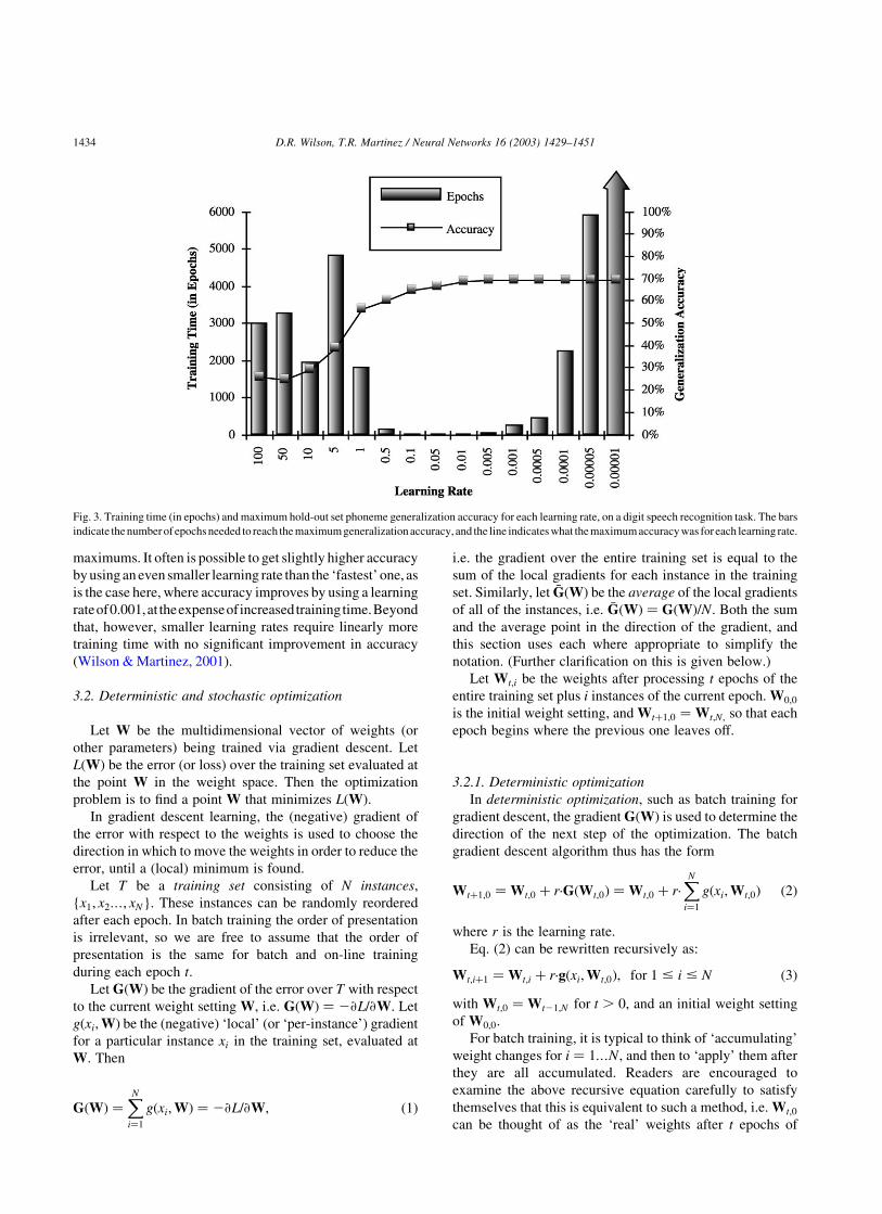
maximums. It often is possible to get slightly higher accuracy

by using an even smaller learning rate than the ‘fastest’ one, as

is the case here, where accuracy improves by using a learning

rateof0.001,at theexpenseofincreasedtrainingtime.Beyond

that, however, smaller learning rates require linearly more

training time with no significant improvement in accuracy

(Wilson & Martinez, 2001).

3.2. Deterministic and stochastic optimization

Let W be the multidimensional vector of weights (or

other parameters) being trained via gradient descent. Let

LðWÞ be the error (or loss) over the training set evaluated at

the point W in the weight space. Then the optimization

problem is to find a point W that minimizes LðWÞ:

In gradient descent learning, the (negative) gradient of

the error with respect to the weights is used to choose the

direction in which to move the weights in order to reduce the

error, until a (local) minimum is found.

Let T be a training set consisting of N instances,

{x1; x2…; xN}: These instances can be randomly reordered

after each epoch. In batch training the order of presentation

is irrelevant, so we are free to assume that the order of

presentation is the same for batch and on-line training

during each epoch t:

Let GðWÞ be the gradient of the error over T with respect

to the current weight setting W; i.e. GðWÞ ¼ 2›L=›W: Let

gðxi;WÞ be the (negative) ‘local’ (or ‘per-instance’) gradient

for a particular instance xi in the training set, evaluated at

W: Then

GðWÞ ¼XN

i¼1

gðxi;WÞ ¼ 2›L=›W; ð1Þ

i.e. the gradient over the entire training set is equal to the

sum of the local gradients for each instance in the training

set. Similarly, let �GðWÞ be the average of the local gradients

of all of the instances, i.e. �GðWÞ ¼ GðWÞ=N: Both the sum

and the average point in the direction of the gradient, and

this section uses each where appropriate to simplify the

notation. (Further clarification on this is given below.)

Let Wt;i be the weights after processing t epochs of the

entire training set plus i instances of the current epoch. W0;0

is the initial weight setting, and Wtþ1;0 ¼ Wt;N; so that each

epoch begins where the previous one leaves off.

3.2.1. Deterministic optimization

In deterministic optimization, such as batch training for

gradient descent, the gradient GðWÞ is used to determine the

direction of the next step of the optimization. The batch

gradient descent algorithm thus has the form

Wtþ1;0 ¼ Wt;0 þ r·GðWt;0Þ ¼ Wt;0 þ r·XN

i¼1

gðxi;Wt;0Þ ð2Þ

where r is the learning rate.

Eq. (2) can be rewritten recursively as:

Wt;iþ1 ¼ Wt;i þ r·gðxi;Wt;0Þ; for 1 # i # N ð3Þ

with Wt;0 ¼ Wt21;N for t . 0; and an initial weight setting

of W0;0:

For batch training, it is typical to think of ‘accumulating’

weight changes for i ¼ 1…N; and then to ‘apply’ them after

they are all accumulated. Readers are encouraged to

examine the above recursive equation carefully to satisfy

themselves that this is equivalent to such a method, i.e. Wt;0

can be thought of as the ‘real’ weights after t epochs of

Fig. 3. Training time (in epochs) and maximum hold-out set phoneme generalization accuracy for each learning rate, on a digit speech recognition task. The bars

indicate the number of epochs needed to reach the maximum generalization accuracy, and the line indicates what the maximum accuracy was for each learning rate.

D.R. Wilson, T.R. Martinez / Neural Networks 16 (2003) 1429–14511434

training, and as can be seen from the equation, Wt;0 is what

is always used to calculate the local gradient for each

instance. Wt;1 through Wt;N are thus not used in the equation

except to accumulate the weight changes.

3.2.2. Stochastic optimization

In stochastic optimization (Kiefer & Wolfowitz, 1952;

Robbins & Monro, 1951; Spall, 1999), on the other hand, an

estimate YðWÞ of the gradient is used at each step. The

Robbins-Monro Stochastic Approximation (RMSA) algor-

ithm (Robbins & Monro, 1951) has the form

Wt;iþ1 ¼ Wt;i þ rk·YðWt;iÞ ð4Þ

where rk is the learning rate after processing k instances, i.e.

k ¼ tN þ i:

Convergence can often be guaranteed if rk decays

according to certain constraints.2 Even when a constant

step size is used, a partial convergence theory is often

possible (Spall, 1999) to within some error of the local

minimum. In our experiments, we have seen slight

improvements in solutions obtained by using a decaying

learning rate, so in practice this is often useful. However, in

order to more directly compare batch and on-line training, a

constant learning rate will be used in the remainder of this

paper.

It would of course be preferable to use the

deterministic gradient �GðWÞ instead of the stochastic

estimate YðWÞ at each step in this optimization, if these

two values took the same amount of time to compute.

However, �GðWÞ takes N times as long to compute as

YðWÞ: As will be shown below, taking N stochastic steps

YðWÞ per epoch actually follows the gradient more

closely and is thus able to make much more progress

than taking a single step in the direction of �GðWÞ:

For on-line training, we use YðWt;iÞ ¼ gðxiþ1;Wt;iÞ; i.e.

the per-instance gradient for each instance is used as an

estimate of the true gradient over the entire training set,

yielding an update equation of:

Wt;iþ1 ¼ Wt;i þ r·gðxiþ1;Wt;iÞ ð5Þ

While it is true that YðWÞ is not equal to �GðWÞ; the

expected value of Y does equal �G (under fairly modest

regularity conditions) (Glasserman, 1991; Spall, 1999). This

is an extremely important point, and so bears repeating:

The expected value of the per-instance gradient used

by on-line training is the true gradient at that point, i.e.

Eðgðxi;WÞÞ ¼ �GðWÞ:

To see that this is so, observe that PðxiÞ ¼ 1=N; since the

instances are presented in random order with equal

probability. Therefore,

Eðgðxi;WÞÞ ¼XN

i¼1

PðxiÞ·gðxi;WÞ ¼XN

i¼1

1

N·gðxi;WÞ

¼1

N

XN

i¼1

gðxi;WÞ ¼GðWÞ

N¼ �GðWÞ ð6Þ

3.3. Why batch training is slower than on-line training

Given the above groundwork, it is now possible to show

why batch training can be expected to be slower than on-line

training, especially as the size of the training set grows large.

3.3.1. Similarity of batch and on-line training

To show more clearly just how similar batch and on-line

training are, the batch and on-line training update equations

(as applied for each instance in the training set) are repeated

below for comparison:

Batch : Wt;iþ1 ¼ Wt;i þ r·gðxi;Wt;0Þ ð3Þ

On-line : Wt;iþ1 ¼ Wt;i þ r·gðxiþ1;Wt;iÞ ð5Þ

From these update equations, it can be seen that the only

difference between the two is that on-line training uses the

weights at the current point in weight space, while batch

uses the weights at the original point in weight space (for

each epoch), when determining how to update the weights

for each instance.

As the learning rate r approaches 0, less change in the

weights is made per epoch, which means that Wt;i ! Wt;0:

Thus batch and on-line training become identical in the limit

as r ! 0: In practice, if the learning rate is small enough for

batch training to follow the gradient closely, on-line

learning will usually follow essentially the same path to

the same minimum.

Some authors define batch training as using the average

of the weight changes over an epoch of N instances

(Principe et al., 2000; Wasserman, 1993) rather than the

sum. These are of course equivalent if one uses a learning

rate of r=N in the former case and r in the latter. However, as

can be seen from the above equations, using the average for

batch training (i.e. r=N) would result in batch training being

N times slower than on-line training in the limit as r ! 0:

We therefore use the sum in batch training in order to make

the comparison fair.

3.3.2. Example of basic difference

Fig. 4(a) shows an example of several individual weight

changes (represented as vectors in 2-space) collected during

2 Convergence under RMSA is guaranteed when (a) rt;i . 0; (b)P1k21 rk ¼ 1; and (c)

P1k21 r2

k , 1; e.g. rk ¼ a=ðk þ 1Þ is a common

choice, though not necessarily optimal for finite training sets (Robbins and

Monro, 1951; Spall, 1999).

D.R. Wilson, T.R. Martinez / Neural Networks 16 (2003) 1429–1451 1435

an epoch of batch training. The long dashed line represents

the sum of these individual vectors and shows the direction

of the true (training set error) gradient.

This sum can also be graphically represented by placing

the same vectors end-to-end, as in Fig. 4(b). When looked at

in this way, batch training can be thought of as ‘updating’ its

weights after each instance, just as in on-line training, but

computing the local gradient at each step with respect to the

original point in weight space, as reflected in the above

equations. In other words, as it travels through weight space

during each epoch, it evaluates each instance at the original

point ðWt;0Þ to decide where it should go from its current

point ðWt;iÞ; even though the gradient may have changed

considerably between those two points.

On-line training, on the other hand, always uses the

current point in weight space Wt;i to compute the local

gradient, and then moves from there. This allows it to follow

curves in the error landscape. Fig. 4(c) illustrates the path of

on-line training for the same instances as in Fig. 4(a) and (b).

It varies from the true gradient at each point by a similar

amount and at a similar angle to the true gradient, but since

it can use the gradient at the current point instead of the

original point, it follows curves and makes much more

progress during the epoch.

In contrast, observe how after the first few steps, batch

training is heading in a general direction that is nearly

perpendicular to the current true gradient. This illustrates

the point that while batch training computes the direction of

the true gradient, this direction is only valid at the starting

point. As the weights actually start to move in that direction,

the direction of the true gradient at the original point is

being used as an estimate of what the gradient is along the

rest of the path. The further along the path the weights get,

the less accurate this estimate becomes.

In on-line training, the path through weight space will

fluctuate around the gradient direction (Principe et al., 2000)

as it curves its way to the minimum, as illustrated earlier in

Fig. 4(c). Batch training, on the other hand, can be thought

of as fluctuating around the fixed gradient calculated at the

original point, as shown by the jagged path taken in

Fig. 4(b). Alternatively, it can be thought of as diverging

from the true gradient in a straight line, as illustrated by the

dashed line in the same figure.

When on-line training makes ‘mistakes’ by overshooting

a minimum, missing a curve, or by moving in a wrong

direction due to its noisy estimate of the gradient, it can start

to make corrections immediately with the very next

instance. This is because each of its stochastic updates is

Fig. 4. Example of changes in weight space. The directed curves indicate the underlying true gradient of the error surface. (a) Batch training. Several weight

change vectors and their sum. (b) Batch training with weight change vectors placed end-to-end. Note that batch training ignores curves and overshoots a ‘valley,’

thus requiring a smaller learning rate. (c) On-line training. The local gradient influences the direction of each weight change vector, allowing it to follow curves.

D.R. Wilson, T.R. Martinez / Neural Networks 16 (2003) 1429–14511436

based on the current gradient at the new point. When batch

training makes mistakes by overshooting a minimum or

failing to follow a curve, it just keeps on going straight until

the beginning of the next epoch.

3.3.3. Neither uses the ‘true’ gradient: both estimate

Thus, both batch and on-line training are using

approximations of the true gradient as they move through

weight space. On-line training uses a rough estimate of the

current gradient at each of N steps during an epoch, while

batch training carefully estimates the gradient at the starting

point, but then ignores any changes in the gradient as it takes

one large step (equivalent to N small average-sized straight

steps) in that direction. Of the two, batch actually tends to

use the less accurate estimate in practice, especially as the

learning rate and/or the size of the training set increases,

since both of these factors increase the distance of the

ending point (where the weights move to) from the initial

point in weight space (where the gradient was calculated).

Even if we knew the optimal size of a step to take in the

direction of the gradient at the current point (which we do

not), we usually would not be at the local minimum, since

the gradient will curve on the way to the minimum. Instead,

we would only be in a position to take a new step in a

somewhat orthogonal direction, as is done in the conjugate

gradient training method (Møller, 1993).

Of course, when using a finite training set, even the true

gradient is in practice the gradient of the training set error

with respect to the weights, not the gradient of the true

underlying function we are trying to approximate, though

this is true for both on-line and batch training.

3.3.4. Brownian motion

Another way to think of on-line training is in terms of

Brownian motion. When a particle exhibits Brownian

motion, it moves in random directions at each point, but is

biased towards moving in the direction of an underlying

current. Similarly, as on-line training progresses, each

weight change can be in any direction, but the probability

distribution is skewed towards the true gradient.

The direction of movement at each point can thus be

looked at as a combination of a noise vector pointing in a

random direction and a gradient vector pointing in the

direction of the true gradient. In the long run, the law of

averages will tend to cancel out much of the noise and push

the weights in the direction of the true gradient. Under this

interpretation, the main difference between batch and on-

line training is that while both will have similar noise

vectors, batch training must use a fixed gradient vector in all

of its weight accumulations for an entire epoch, while on-

line training is allowed to use the current gradient vector for

each of its weight updates.

Put differently, the expected value of the weight change

for each instance is r· �GðWt;iÞ for on-line training and

r· �GðWt;0Þ for batch training. After every N instances (i.e.

one pass through the training set), the expected value of

the weight change for batch training suddenly changes to

point in the direction of the gradient at the end of the

previous epoch, and then remains fixed until the end of the

next epoch. In contrast, the expected value of the weight

change for on-line training is continuously pointing in the

direction of the gradient at the current point in weight space.

This allows it to follow curves in the gradient throughout an

epoch.

3.3.5. Large training sets

As the size of the training set grows, the accumulated

weight changes for batch training become large. For

example, consider a training set with 20,000 instances. If

a learning rate of 0.1 is used, and the average gradient is on

the order of ^0.1 for each weight per instance, then the total

accumulated weight change will be on the order of ^ð0:1 £

0:1 £ 20; 000Þ ¼ ^200: Considering that weights usually

begin with values well within the range of ^1, this

magnitude of weight change is very unreasonable and will

result in wild oscillations across the weight space, and

extreme overshooting of not only the local minima but the

entire area of reasonable solutions.

In networks such as multilayer perceptrons, such large

weight changes will also cause saturation of nonlinear (e.g.

sigmoidal) units, making further progress difficult. In terms

of the hyperplanes or other hypersurfaces constructed by

neural network architectures, such overshooting often

equates to putting all of the data on one side of the

‘decision’ surfaces with nothing on the other side, resulting

in random or nearly random behavior. Thus, a reduction in

the size of the learning rate is required for batch training to

be stable as the size of the training set grows. (This is often

done implicitly by using the average weight change instead

of the sum, effectively dividing the learning rate by N).

On-line learning, on the other hand, applies weight

changes as soon as they are computed, so it can handle any

size of training set without requiring a smaller learning rate.

In the above example, each weight change will be on the

order of ^0:1 £ 0:1 ¼ ^0:01; even with a learning rate of

0.1. If we consider a ‘safe’ step size for this example to be

on the order of ^0.01, then batch might need to use a

learning rate as small as r ¼ 0:1=N ¼ 0:00005 in order to

take steps of that size.

Since some of the individual weight changes cancel each

other out, the learning rate does not usually need to be a full

N times smaller for batch than for on-line, but it does

usually need to be much smaller. In the above example r

would perhaps need to be 200 times smaller, or r ¼

0:1=200 ¼ 0:0005: This in turn means that batch training

will require many more (e.g. 200 times as many) iterations

through the training data when compared to on-line training.

In our experiments it was common to have to reduce the

learning rate by a factor of aroundffiffiffiN

pto get batch training

to train with the same stability as on-line training on a

training set of N instances. This is only a rough estimate,

and the precise relationship between training set size and

D.R. Wilson, T.R. Martinez / Neural Networks 16 (2003) 1429–1451 1437

reduction in learning rate required for batch training is

highly task-dependent. (Of course, once we know that on-

line training is significantly faster than batch and at least as

accurate, it may be less important to know exactly how

much faster it is.)

As the training set gets larger, on-line training can make

more progress within each epoch, while batch training must

make the learning rate smaller (either explicitly or by using

the average weight change) so as not to go too far in a straight

line. With a sufficiently large training set, on-line training

will converge in less than one epoch before batch training

takes its first step. In the limit, with an infinite training set,

batch training would never take a step while on-line training

would converge as usual.

3.4. Choosing a learning rate

One concern that might arise is that even if on-line

training can use a larger learning rate than batch training,

there is in general no way of knowing what size of learning

rate to use for a particular task, and so there is no guarantee

of finding the larger learning rate that would allow on-line

training to learn faster. However, both on-line and batch

training share this problem, so this cannot be seen as a

comparative disadvantage to on-line training. In fact, since

on-line training can use a larger learning rate, the search for

an appropriate learning rate is easier with on-line training,

since the entire range of learning rates safe for use in batch

training are also available for on-line training, as well as an

additional range of larger rates. Furthermore, since these

larger learning rates allow for faster training, the process of

searching for learning rates itself can be sped up, because

larger learning rates can be quickly checked and smaller

ones can then be more quickly ruled out as they fail to

improve upon earlier results.

With on-line training, ‘the weight vector never settles

to a stable value’ (Reed & Marks, 1999), because the

local gradients are often non-zero even when the true

gradient is zero. The learning rate is therefore sometimes

decayed over time (Bishop, 1997). In our experiments we

held the learning rates constant throughout training so that

comparisons of training time would be more meaningful,

but it might be advantageous to reduce the learning rate

after approximate convergence has been reached (Reed &

Marks, 1999).

3.5. Momentum

The experiments in this paper have not used the

momentum term. When the momentum term is used, the

process is no longer gradient descent anyway, though it has

in some cases sped up the learning process. Given a

momentum term of a; with 0 # a # 1; the effective

learning rate is ra ¼ r=ð1 2 aÞ when weight changes are

in approximately the same direction. Momentum can thus

have an amplification effect on the learning rate, which

would tend to hurt batch training more than on-line training.

Momentum can also help to ‘cancel out’ steps taken in

somewhat opposite directions, as when stepping back and

forth across a valley. In such cases the unproductive

elements tend to cancel out, while the common portions

tend to add to each other.

We ran just a few experiments using momentum, and

from these it appeared that on-line retained the same

advantage over batch in terms of speed and smoothness of

learning, and that indeed the learning rate was amplified

slightly. On the Australian task, for example, using a

momentum of a ¼ 0:9 and a learning rate of r ¼ 0:001

resulted in training similar to using a learning rate between

r ¼ 0:001 and r ¼ 0:01 for both batch and on-line training.

3.6. Batch/on-line hybrid

Another approach we tried was to do on-line training for

the first few epochs to get the weights into a reasonable

range and follow this by batch training. Although this helps

to some degree over batch training, empirical results and

analytical examination show that this approach still requires

a smaller learning rate and is thus slower than on-line

training, with no demonstrated gain in accuracy.

Basically, such a hybrid approach is the same as on-line

training until the epoch at which batch training begins, and

then must use the same small learning rate as when batch

training is used alone in order to do stable learning.

4. Empirical results

From the discussions in preceding sections, we hypoth-

esized that on-line training is usually faster than batch

training, especially for large training sets, because it can

safely use a larger learning rate, due to its ability to follow

curves in the error surface. However, how much faster on-

line is depends on both the size of the training set and the

characteristics of the particular application. As discussed

above, as the training set gets larger, we expect the speedup

of on-line over batch to increase.

The smoothness of the underlying error surface also

influences training speed. A smoother surface usually

allows a larger learning rate which typically allows faster

convergence. However, since both on-line and batch

training can use a larger learning rate on a smoother

surface, smoothness may not have as much effect as other

factors on speedup.

The amount of speedup of on-line over batch also

depends on how much cooperation there is among the ‘local

gradients’ of the individual training instances. If the

individual weight changes for all N instances in the training

set happen to be in the direction of the true (current)

gradient, then on-line training would be able to progress N

times as fast as the corresponding batch algorithm, since it

D.R. Wilson, T.R. Martinez / Neural Networks 16 (2003) 1429–14511438

could make the same progress per instances as batch would

per epoch.

On the other hand, the individual on-line training steps

could be so contradictory that the total amount of progress

made in an entire epoch is less than or equal to the size of a

typical single step in on-line training. This case can be

thought of as N 2 1 steps canceling each other out, leaving

one final step (or partial step) of actual progress in the

direction of the true gradient. Alternatively, it can be

thought of as N steps, each of which moves only 1=N of a

full step or less in the right direction (on average). Either

way, the additional steps taken by on-line training in such

situations are ‘wasted’ (though no more so than the similar

accumulations made by batch) so training is reduced to

being no faster than batch training.

In more realistic cases, we expect there to be some

contradiction between the weight changes for individual

training instances because they each favor their own output

values, but also some cooperation among many instances in

the direction of the true gradient. Determining the amount of

such cooperation analytically is very difficult for real-world

tasks, and it varies widely depending on the characteristics

of each task. Therefore, empirical results are needed to

explore the question of how much faster on-line is than

batch training in practice.

Two sets of experiments were run, one using a collection

of classification tasks with various sizes of training sets, and

another using a large training set for a speech recognition

task. In both cases various learning rates were used for on-

line and batch training. In the speech recognition task, mini-

batch training was also used with various update frequencies

(‘batch sizes’) to further explore the relationship between

batch size, learning rate, and training speed.

The experiments in this paper use multilayer perceptrons

(MLP) trained using the error backpropagation (BP)

algorithm (Rumelhart & McClelland, 1986).

4.1. Machine learning database experiments

One problem with earlier comparisons between batch

and on-line training is that they have used a single learning

rate to compare the two, ignoring the fact that on-line

training can often use a larger learning rate than batch

training. Another problem is that they often used artificial

and/or ‘toy’ (very small, simple) problems for comparison,

thus missing differences that occur in larger problems.

In order to test the hypothesis that on-line training trains

faster than batch training, experiments were run on 26

classification tasks from the UCI Repository of Machine

Learning Databases (Blake & Merz, 1998). For each task,

60% of the data was used for training, 20% for a hold-out

set, and the remaining 20% as a final test set. The hold-out

set was used to test the generalization accuracy after each

epoch of training, and the final test set was used to measure

accuracy at the epoch where generalization was the highest

on the hold-out set.

Each task was trained using both on-line and batch

training methods, and in each case learning rates of 0.1,

0.01, 0.001, and 0.0001 were used. Ten trials were run for

each of the four learning rates for both methods on each of

the 26 tasks, for a total of 10 £ 4 £ 2 £ 26 ¼ 2080 runs:

Each run used error backpropagation to train a multilayer

perceptron. For a classification task with X inputs and Z

output classes, the architecture of the multilayer perceptron

was set up to have X input nodes, one layer of X £ 2 hidden

nodes, and Z output nodes. During training the target value

of the output node corresponding to the target output class

was set to 1, and the target value of the other nodes was set

to 0. During testing, an instance was considered to be

classified correctly if the target output class had the highest

activation of any of the output nodes. The generalization

accuracy on the hold-out and test set was defined the

percentage of instances correctly classified in the hold-out

or test set, respectively.

The neural networks in each experiment were initi-

alized with small random weights, and the order of

presentation of instances was randomized such that it was

different for each epoch. The random number generator

was seeded with a number that was determined by which

of the ten trials the experiment was in. Thus, each of the

ten trials started with different random initial weights, but

the batch and on-line methods for each experiment always

used the same random initial weights for each of their

corresponding trials. Similarly, each of the ten trials used

the same random initial weights for all four learning rates,

and used the same order of presentation of instances for

both on-line and batch training as well as for the four

different learning rates.

Each neural network was trained for 1000 epochs for

learning rates 0.1 and 0.01; 5000 epochs for 0.001; and 10,000

epochs for learning rate 0.0001. Each neural network was then

tested on the hold-out set and the results for each epoch over

the ten trials were averaged. A few tasks had generalization

accuracy that was still rising after the number of epochs listed

above. In those cases, additional training epochs were used in

order to determine how long batch and on-line training took to

train to a maximum accuracy in each case.

We first show a representative example of the behavior of

batch and on-line training in detail, and then discuss the

average results over all 26 tasks.

4.1.1. Example: Mushroom

The Mushroom dataset has 3386 instances in its

training set, and generalization accuracy after each

epoch is plotted in Fig. 5 for the four learning rates. As

shown in Fig. 5(a), for a learning rate of 0.1, on-line

training fluctuates on its way to an asymptote at about

98.5% accuracy, which it reaches after about 800 epochs,

while batch training remains completely random. In Fig.

5(b), a learning rate of 0.01 allows on-line training to

D.R. Wilson, T.R. Martinez / Neural Networks 16 (2003) 1429–1451 1439

smoothly approach 100% generalization accuracy after

only 20 epochs, while batch training continues to remain

random. In Fig. 5(c), batch training finally makes some

progress with a learning rate of 0.001, but still achieves

only a 98.5% accuracy after 3800 epochs. Finally, with a

learning rate of 0.0001, batch training follows on-line

training quite closely, as shown in Fig. 5(d), dipping only

slightly a few times, and both reach 100% accuracy after

about 1800 epochs.

In this example, batch training required 1800 epochs to

reach 100% using its best learning rate of 0.0001, while on-

line training was able to do so in 20 epochs using a learning

rate of 0.01.

In this case it is easy to see that if someone used a

learning rate small enough for batch training to converge—

i.e. 0.0001—and compared batch and on-line training using

this same learning rate, they might conclude that there is no

significant difference between the two. But since on-line

learning can use a larger learning rate, it is in fact able to

learn 90 times as fast in this case.

It is common for people to use the average weight

change in batch training instead of the sum. With a learning

rate of r £ N ¼ 0:0001 £ 3386 ¼ 0:3386; taking the average

would yield the exact same results as using the sum with a

learning rate of 0.0001. This agrees with the rule of thumb

of Principe et al. (2000), as mentioned in Section 2.1, that

when using the average weight change, batch training can

use a learning rate that is an order of magnitude larger than

on-line training (0.3386 vs. 0.01, in this case, to achieve

smooth learning). Regardless of whether the sum (with

learning rate 0.0001) or the average (with learning rate of

0.3386) is used, however, the result is the same: batch

training requires 90 times as many iterations as on-line

training when both are allowed to use their ‘best’ learning

rate.

In the remainder of this paper, the sum is used, because

using the sum has the property that as the learning rate

becomes small, batch and on-line training become

equivalent.

4.1.2. Overall results

Fig. 6 shows the average accuracy of all 26 tasks after

each epoch of training for the same learning rates. For

learning rates of 0.1, 0.01, 0.001 and 0.0001, batch training

is on average about 30, 12.5, 4 and 0.8% lower than on-line

training, respectively, at any particular epoch. This shows

again that the smaller the learning rate is, the more closely

batch and on-line training behave. It also demonstrates that

on-line training generally learns more quickly (as well as

more ‘safely’) with larger learning rates. The small

difference observed in Fig. 6(d) is almost entirely due to

the Letter Recognition task which has 12,000 instances in

Fig. 5. Generalization accuracy of on-line and batch training on the Mushroom task, using learning rates of (a) 0.1, (b) 0.01, (c) 0.001, and (d) 0.0001.

D.R. Wilson, T.R. Martinez / Neural Networks 16 (2003) 1429–14511440

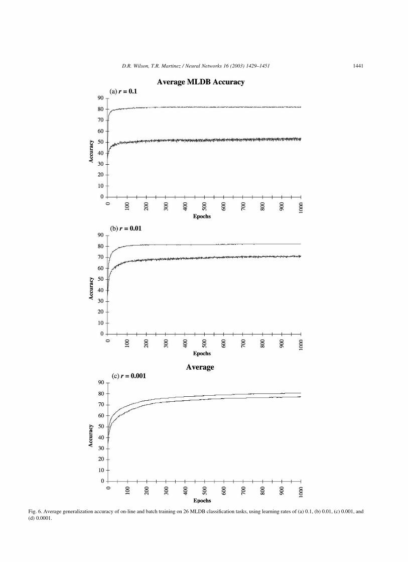
Fig. 6. Average generalization accuracy of on-line and batch training on 26 MLDB classification tasks, using learning rates of (a) 0.1, (b) 0.01, (c) 0.001, and

(d) 0.0001.

D.R. Wilson, T.R. Martinez / Neural Networks 16 (2003) 1429–1451 1441

the training set. For that task, a learning rate of 0.0001 was

still too large for batch training, though on-line training did

fine with a learning rate of 0.001.

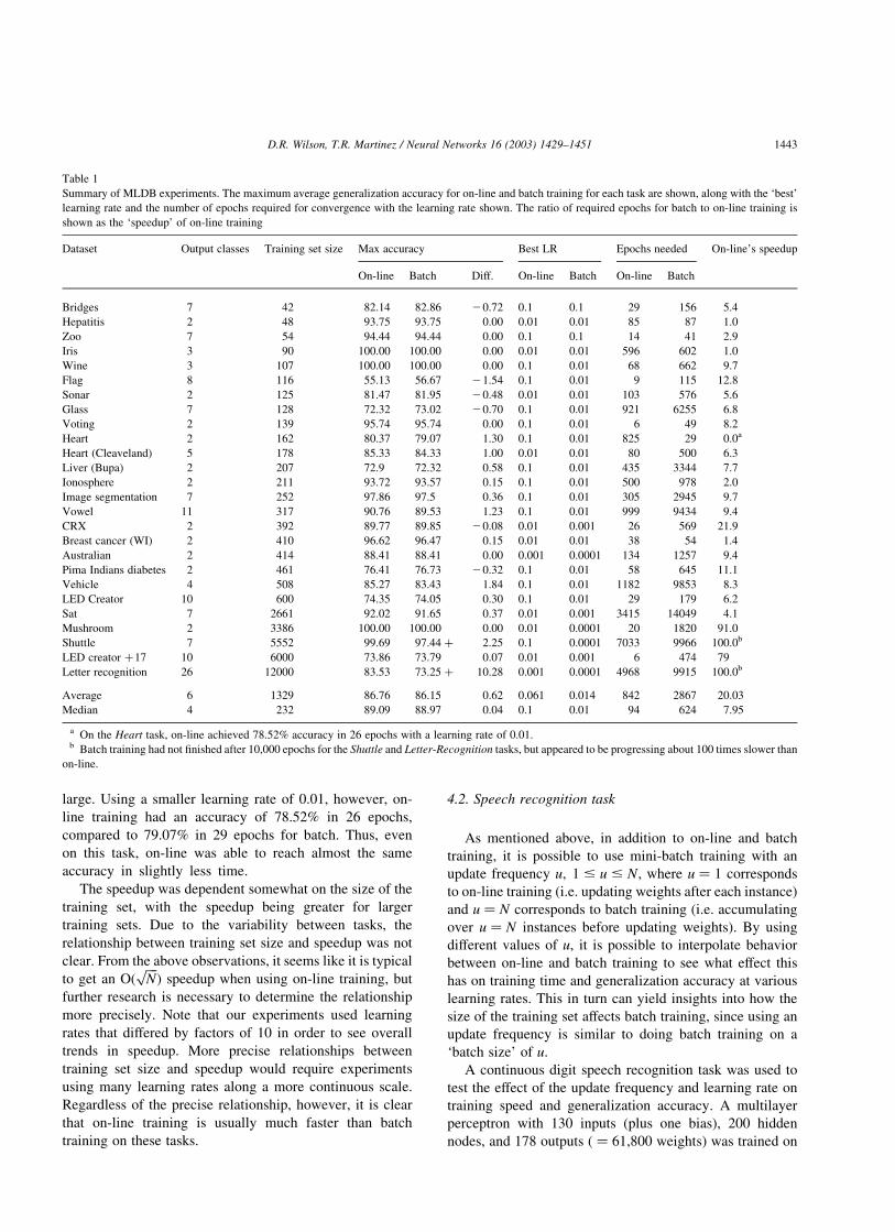
Table 1 summarizes the experiments on all of the

Machine Learning Databases. The first two columns after

the task’s name show how many output classes each

database had and the number of instances in the training set.

The tasks are sorted by the size of the training set.

The main question was how long it took to train each task

using on-line vs. batch training. To determine this for each

task, the following steps were taken. For each learning rate r

in {0.1, 0.01, 0.001, 0.0001} and method m in {on-line,

batch}, the average generalization accuracy on the hold-out

set for all 10 trials after each training epoch was recorded, as

was done for the Mushroom example in Fig. 5. The

maximum accuracy for each such run was recorded, along

with the number of epochs required to achieve that accuracy

and the additional test set accuracy at that epoch.

Space does not allow the presentation of all of these

results, but they are available in the on-line appendix (see

Appendix A of this paper). Instead, the highest accuracy

achieved by each method for any learning rate is shown

under the heading ‘Max Accuracy’ in Table 1. The

difference between the maximum accuracy for the on-line

and batch training methods is shown under the heading

‘Diff.’

The ‘best’ learning rate was chosen to be the one that

used the fewest number of training epochs to get within

0.5% of the maximum accuracy achieved on that task by the

respective method. For example, in the Pima Indians

Diabetes task, on-line training achieved an accuracy of

76.41% after 287 epochs with a learning rate of 0.01, but

required 7,348 epochs to reach a maximum of 76.51% with

a learning rate of 0.0001. The difference in accuracy is not

significant, but the difference in training time is dramatic, so

the idea is to choose whichever learning rate achieves

a reasonably good solution most quickly rather than

depending so heavily on minor accuracy fluctuations.

On the other hand, on many tasks the maximum accuracy

reached with a large learning rate was very poor, so such

learning rates could not be considered best even though they

reached their (poor) maximum very quickly. For example,

on the Mushroom task, batch training achieved a maximum

accuracy of 58.9% in just 2 epochs with a learning rate of

0.1, but was able to get 100% accuracy in 1852 epochs using

a learning rate of 0.0001. In this case we obviously prefer

the learning rate which produces substantially higher

accuracy, even if it is much slower.

The best learning rate for each task is shown under the

column ‘Best LR’ in Table 1. The number of epochs needed

to reach the maximum accuracy by the best learning rate for

each method is shown under the heading ‘Epochs Needed.’

The last column of Table 1 shows what the speedup of

on-line training was over batch training, which is how many

times faster on-line training was than batch training on that

task. The Shuttle and Letter Recognition tasks both required

more than 10,000 epochs for batch training to converge. In

both cases, plotting the results up to 10,000 epochs on a

logarithmic scale showed that the best learning rate for

batch training was progressing approximately 100 times

slower than on-line training. It was not practical to run these

tasks for the estimated 500,000–10,000,000 epochs they

would need to reach their maximum.

On this set of 26 applications, on-line training was an

average of over 20 times as fast as batch training. On

applications with over 1000 training instances, on-line

training was over 70 times as fast as batch training on

average. On-line training was faster on all but one of the

tasks in this set of tasks. In that one case, the Heart task,

on-line training had a generalization accuracy that was

1.3% higher than batch, but required 825 epochs to

achieve this, indicating that a learning rate of 0.1 is too

Fig. 6 (Continued)

D.R. Wilson, T.R. Martinez / Neural Networks 16 (2003) 1429–14511442

large. Using a smaller learning rate of 0.01, however, on-

line training had an accuracy of 78.52% in 26 epochs,

compared to 79.07% in 29 epochs for batch. Thus, even

on this task, on-line was able to reach almost the same

accuracy in slightly less time.

The speedup was dependent somewhat on the size of the

training set, with the speedup being greater for larger

training sets. Due to the variability between tasks, the

relationship between training set size and speedup was not

clear. From the above observations, it seems like it is typical

to get an OðffiffiffiN

pÞ speedup when using on-line training, but

further research is necessary to determine the relationship

more precisely. Note that our experiments used learning

rates that differed by factors of 10 in order to see overall

trends in speedup. More precise relationships between

training set size and speedup would require experiments

using many learning rates along a more continuous scale.

Regardless of the precise relationship, however, it is clear

that on-line training is usually much faster than batch

training on these tasks.

4.2. Speech recognition task

As mentioned above, in addition to on-line and batch

training, it is possible to use mini-batch training with an

update frequency u; 1 # u # N; where u ¼ 1 corresponds

to on-line training (i.e. updating weights after each instance)

and u ¼ N corresponds to batch training (i.e. accumulating

over u ¼ N instances before updating weights). By using

different values of u; it is possible to interpolate behavior

between on-line and batch training to see what effect this

has on training time and generalization accuracy at various

learning rates. This in turn can yield insights into how the

size of the training set affects batch training, since using an

update frequency is similar to doing batch training on a

‘batch size’ of u:

A continuous digit speech recognition task was used to

test the effect of the update frequency and learning rate on

training speed and generalization accuracy. A multilayer

perceptron with 130 inputs (plus one bias), 200 hidden

nodes, and 178 outputs ( ¼ 61,800 weights) was trained on

Table 1

Summary of MLDB experiments. The maximum average generalization accuracy for on-line and batch training for each task are shown, along with the ‘best’

learning rate and the number of epochs required for convergence with the learning rate shown. The ratio of required epochs for batch to on-line training is

shown as the ‘speedup’ of on-line training

Dataset Output classes Training set size Max accuracy Best LR Epochs needed On-line’s speedup

On-line Batch Diff. On-line Batch On-line Batch

Bridges 7 42 82.14 82.86 20.72 0.1 0.1 29 156 5.4

Hepatitis 2 48 93.75 93.75 0.00 0.01 0.01 85 87 1.0

Zoo 7 54 94.44 94.44 0.00 0.1 0.1 14 41 2.9

Iris 3 90 100.00 100.00 0.00 0.01 0.01 596 602 1.0

Wine 3 107 100.00 100.00 0.00 0.1 0.01 68 662 9.7

Flag 8 116 55.13 56.67 21.54 0.1 0.01 9 115 12.8

Sonar 2 125 81.47 81.95 20.48 0.01 0.01 103 576 5.6

Glass 7 128 72.32 73.02 20.70 0.1 0.01 921 6255 6.8

Voting 2 139 95.74 95.74 0.00 0.1 0.01 6 49 8.2

Heart 2 162 80.37 79.07 1.30 0.1 0.01 825 29 0.0a

Heart (Cleaveland) 5 178 85.33 84.33 1.00 0.01 0.01 80 500 6.3

Liver (Bupa) 2 207 72.9 72.32 0.58 0.1 0.01 435 3344 7.7

Ionosphere 2 211 93.72 93.57 0.15 0.1 0.01 500 978 2.0

Image segmentation 7 252 97.86 97.5 0.36 0.1 0.01 305 2945 9.7

Vowel 11 317 90.76 89.53 1.23 0.1 0.01 999 9434 9.4

CRX 2 392 89.77 89.85 20.08 0.01 0.001 26 569 21.9

Breast cancer (WI) 2 410 96.62 96.47 0.15 0.01 0.01 38 54 1.4

Australian 2 414 88.41 88.41 0.00 0.001 0.0001 134 1257 9.4

Pima Indians diabetes 2 461 76.41 76.73 20.32 0.1 0.01 58 645 11.1

Vehicle 4 508 85.27 83.43 1.84 0.1 0.01 1182 9853 8.3

LED Creator 10 600 74.35 74.05 0.30 0.1 0.01 29 179 6.2

Sat 7 2661 92.02 91.65 0.37 0.01 0.001 3415 14049 4.1

Mushroom 2 3386 100.00 100.00 0.00 0.01 0.0001 20 1820 91.0

Shuttle 7 5552 99.69 97.44 þ 2.25 0.1 0.0001 7033 9966 100.0b

LED creator þ17 10 6000 73.86 73.79 0.07 0.01 0.001 6 474 79

Letter recognition 26 12000 83.53 73.25 þ 10.28 0.001 0.0001 4968 9915 100.0b

Average 6 1329 86.76 86.15 0.62 0.061 0.014 842 2867 20.03

Median 4 232 89.09 88.97 0.04 0.1 0.01 94 624 7.95

a On the Heart task, on-line achieved 78.52% accuracy in 26 epochs with a learning rate of 0.01.b Batch training had not finished after 10,000 epochs for the Shuttle and Letter-Recognition tasks, but appeared to be progressing about 100 times slower than

on-line.

D.R. Wilson, T.R. Martinez / Neural Networks 16 (2003) 1429–1451 1443

a training set of N ¼ 20; 000 training instances. The output

class of each instance corresponded to one of 178 context-

dependent phoneme categories from a digit vocabulary. For

each instance, one of the 178 outputs had a target of 1, and

all other outputs had a target of 0. The targets of each

instance were derived from hand-labeled phoneme rep-

resentations of a set of training utterances.

To measure the accuracy of the neural network, a hold-

out set of 135 multi-digit speech utterances was run through

a speech recognition system, for a total of 542 digit ‘words.’

The system extracted 130 input features per 10 ms frame

from the speech signal and fed them into the trained neural

network which in turn output a probability estimate for each

of the 178 context-dependent phoneme categories on each

of the frames. A dynamic programming decoder then

searched the sequence of output vectors to find the most

probable word sequence allowed by the vocabulary and

grammar.

The word (digit) sequence generated by the recognizer

was compared with the true (target) sequence of digits, and

a dynamic programming algorithm was used to determine

the number of correct matches, insertions, deletions, and

substitutions in the utterance. The generalization word

accuracy was computed as the percentage of correctly

recognized words minus the percentage of additional

inserted words, as is typical in speech recognition

experiments (Rabiner & Juang, 1993).

Mini-batch training was done with update frequencies of

u ¼ 1 (i.e. on-line training), 10, 100, 1000, and 20,000 (i.e.

batch training). Learning rates of r ¼ 0:1; 0:01; 0:001; and

0.0001 were used with appropriate values of u in order to see

how small the learning rate needed to be to allow each size

of mini-batch training to learn properly.

For each training run, the generalization word accuracy

was measured after each training epoch so that the progress

of the network could be plotted over time. Each training run

used the same set of random initial weights (i.e. using the

same random number seed), and the same random

presentation orders of the training instances for each

corresponding epoch.

Training on 20,000 instances with 61,800 weights took

much longer per epoch than any of the Machine Learning

Database tasks, so it was not practical to run 10 trials of each

series (i.e. each learning rate and batch size). Therefore,

only one trial was run for each series. Furthermore, each

series was run for up to 5000 epochs, but was stopped early

if it appeared that the maximum accuracy had already been

reached.

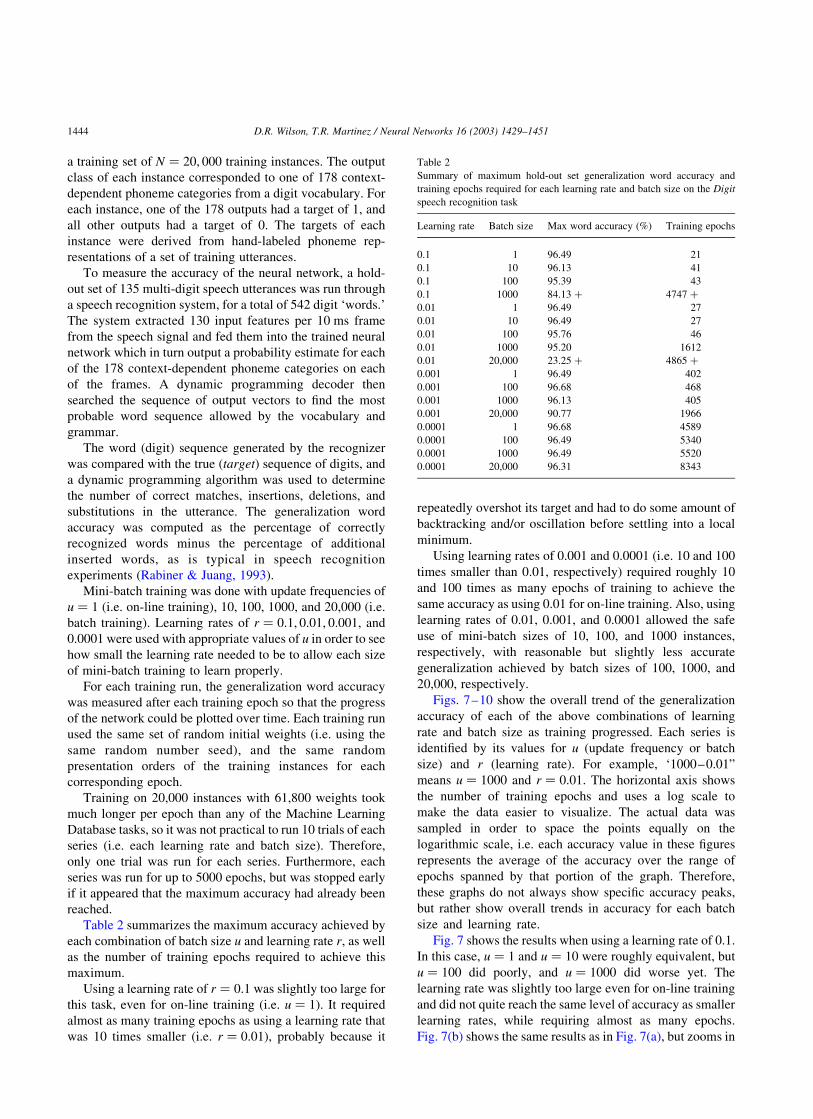
Table 2 summarizes the maximum accuracy achieved by

each combination of batch size u and learning rate r; as well

as the number of training epochs required to achieve this

maximum.

Using a learning rate of r ¼ 0:1 was slightly too large for

this task, even for on-line training (i.e. u ¼ 1). It required

almost as many training epochs as using a learning rate that

was 10 times smaller (i.e. r ¼ 0:01), probably because it

repeatedly overshot its target and had to do some amount of

backtracking and/or oscillation before settling into a local

minimum.

Using learning rates of 0.001 and 0.0001 (i.e. 10 and 100

times smaller than 0.01, respectively) required roughly 10

and 100 times as many epochs of training to achieve the

same accuracy as using 0.01 for on-line training. Also, using

learning rates of 0.01, 0.001, and 0.0001 allowed the safe

use of mini-batch sizes of 10, 100, and 1000 instances,

respectively, with reasonable but slightly less accurate

generalization achieved by batch sizes of 100, 1000, and

20,000, respectively.

Figs. 7–10 show the overall trend of the generalization

accuracy of each of the above combinations of learning

rate and batch size as training progressed. Each series is

identified by its values for u (update frequency or batch

size) and r (learning rate). For example, ‘1000–0.01”

means u ¼ 1000 and r ¼ 0:01: The horizontal axis shows

the number of training epochs and uses a log scale to

make the data easier to visualize. The actual data was

sampled in order to space the points equally on the

logarithmic scale, i.e. each accuracy value in these figures

represents the average of the accuracy over the range of

epochs spanned by that portion of the graph. Therefore,

these graphs do not always show specific accuracy peaks,

but rather show overall trends in accuracy for each batch

size and learning rate.

Fig. 7 shows the results when using a learning rate of 0.1.

In this case, u ¼ 1 and u ¼ 10 were roughly equivalent, but

u ¼ 100 did poorly, and u ¼ 1000 did worse yet. The

learning rate was slightly too large even for on-line training

and did not quite reach the same level of accuracy as smaller

learning rates, while requiring almost as many epochs.

Fig. 7(b) shows the same results as in Fig. 7(a), but zooms in

Table 2

Summary of maximum hold-out set generalization word accuracy and

training epochs required for each learning rate and batch size on the Digit

speech recognition task

Learning rate Batch size Max word accuracy (%) Training epochs

0.1 1 96.49 21

0.1 10 96.13 41

0.1 100 95.39 43

0.1 1000 84.13 þ 4747 þ

0.01 1 96.49 27

0.01 10 96.49 27

0.01 100 95.76 46

0.01 1000 95.20 1612

0.01 20,000 23.25 þ 4865 þ

0.001 1 96.49 402

0.001 100 96.68 468

0.001 1000 96.13 405

0.001 20,000 90.77 1966

0.0001 1 96.68 4589

0.0001 100 96.49 5340

0.0001 1000 96.49 5520

0.0001 20,000 96.31 8343

D.R. Wilson, T.R. Martinez / Neural Networks 16 (2003) 1429–14511444

on the higher accuracy range in order to show where there

are subtle differences in accuracy between u ¼ 1 and u ¼

10: Batch training was so slow for this learning rate that it

was not plotted.

As shown in Fig. 8, when using the learning rate r ¼

0:01; u ¼ 1 and u ¼ 10 performed almost identically,

achieving an accuracy of 96.49% after 27 epochs. Using

u ¼ 100 was close but not quite as good (95.76% after 46

epochs), and u ¼ 1000 did poorly (i.e. it took over 1500

epochs to achieve its maximum accuracy of 95.02%). Batch

training performed no better than random for over 100 epochs

and did not get above 17.2% accuracy after 5000 epochs.

Fig. 9 shows that for r ¼ 0:001; u ¼ 1 and u ¼ 100

performed almost identically, achieving close to the same

Fig. 7. Generalization accuracy on the Digit speech recognition task, using a learning rate of 0.1. Each series represents a different mini-batch update frequency

(1 ¼ on-line, ‘1000–0.1’ accumulates changes over 1000 instances before updating weights).

D.R. Wilson, T.R. Martinez / Neural Networks 16 (2003) 1429–1451 1445

accuracy after about 400 epochs. (Since u ¼ 10 is between

u ¼ 1 and u ¼ 100; which are almost identical for this

learning rate, it is excluded for the sake of simplicity.) Using

u ¼ 1000 caused a slight drop in accuracy, though it was

close to the smaller values of u: As seen in Fig. 9(b),

u ¼1000 followed a different path than the other two. Full

batch training (i.e. u ¼ 20; 000) training did poorly, taking

five times as long (1966 epochs) to reach a maximum

accuracy of only 90.77%.

Finally, using r ¼ 0:0001; u ¼ 1; u ¼ 100; and �

u ¼ 1000 all performed almost identically, as shown in

Fig. 10, achieving an accuracy of 96.31% after about 5000

Fig. 8. Generalization accuracy on the Digit speech recognition task, using a learning rate of 0.01. Each series represents a different mini-batch update

frequency (1 ¼ on-line, 20 k ¼ batch).

D.R. Wilson, T.R. Martinez / Neural Networks 16 (2003) 1429–14511446

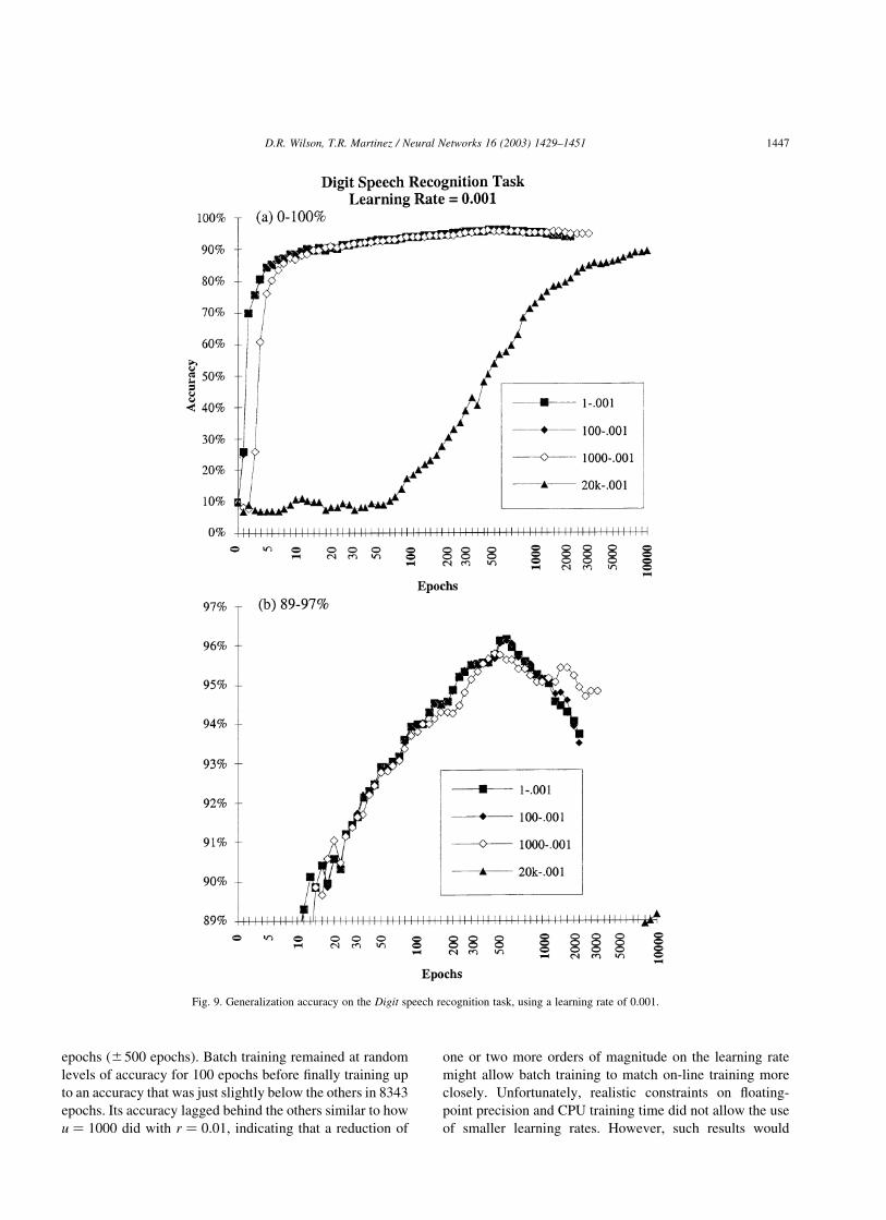
epochs (^500 epochs). Batch training remained at random

levels of accuracy for 100 epochs before finally training up

to an accuracy that was just slightly below the others in 8343

epochs. Its accuracy lagged behind the others similar to how

u ¼ 1000 did with r ¼ 0:01; indicating that a reduction of

one or two more orders of magnitude on the learning rate

might allow batch training to match on-line training more

closely. Unfortunately, realistic constraints on floating-

point precision and CPU training time did not allow the use

of smaller learning rates. However, such results would

Fig. 9. Generalization accuracy on the Digit speech recognition task, using a learning rate of 0.001.

D.R. Wilson, T.R. Martinez / Neural Networks 16 (2003) 1429–1451 1447

contribute little to the overall conclusions of the impracti-

cality of batch training on large training sets.

Table 3 gives an overall summary showing how many

training epochs were required to train the neural network

using the best learning rate for each batch size u. In this

table, the accuracy reported is that achieved on the test set,

which was separate from the hold-out set used in Figs. 7–10

and Table 2. Table 3 shows that eventually, on-line,

mini-batch and batch were able to achieve the same

generalization accuracy, but that batch training required

over 300 times as many epochs to do so.

These results illustrate that as soon as the learning rate is

small enough to avoid drastic overshooting of curves and

local minima, there is a linear relationship between

Fig. 10. Generalization accuracy on the Digit speech recognition task, using a learning rate of 0.0001.

D.R. Wilson, T.R. Martinez / Neural Networks 16 (2003) 1429–14511448

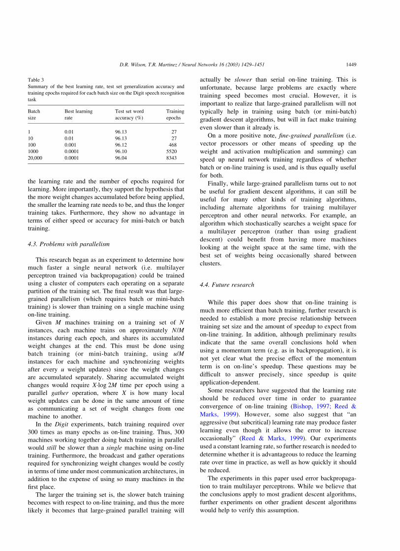
the learning rate and the number of epochs required for

learning. More importantly, they support the hypothesis that

the more weight changes accumulated before being applied,

the smaller the learning rate needs to be, and thus the longer

training takes. Furthermore, they show no advantage in

terms of either speed or accuracy for mini-batch or batch

training.

4.3. Problems with parallelism

This research began as an experiment to determine how

much faster a single neural network (i.e. multilayer

perceptron trained via backpropagation) could be trained

using a cluster of computers each operating on a separate

partition of the training set. The final result was that large-

grained parallelism (which requires batch or mini-batch

training) is slower than training on a single machine using

on-line training.

Given M machines training on a training set of N

instances, each machine trains on approximately N=M

instances during each epoch, and shares its accumulated

weight changes at the end. This must be done using

batch training (or mini-batch training, using u=M

instances for each machine and synchronizing weights

after every u weight updates) since the weight changes

are accumulated separately. Sharing accumulated weight

changes would require X·log 2M time per epoch using a

parallel gather operation, where X is how many local

weight updates can be done in the same amount of time

as communicating a set of weight changes from one

machine to another.

In the Digit experiments, batch training required over

300 times as many epochs as on-line training. Thus, 300

machines working together doing batch training in parallel

would still be slower than a single machine using on-line

training. Furthermore, the broadcast and gather operations

required for synchronizing weight changes would be costly

in terms of time under most communication architectures, in

addition to the expense of using so many machines in the

first place.

The larger the training set is, the slower batch training

becomes with respect to on-line training, and thus the more

likely it becomes that large-grained parallel training will

actually be slower than serial on-line training. This is

unfortunate, because large problems are exactly where

training speed becomes most crucial. However, it is

important to realize that large-grained parallelism will not

typically help in training using batch (or mini-batch)

gradient descent algorithms, but will in fact make training

even slower than it already is.

On a more positive note, fine-grained parallelism (i.e.

vector processors or other means of speeding up the

weight and activation multiplication and summing) can

speed up neural network training regardless of whether

batch or on-line training is used, and is thus equally useful

for both.

Finally, while large-grained parallelism turns out to not

be useful for gradient descent algorithms, it can still be

useful for many other kinds of training algorithms,

including alternate algorithms for training multilayer

perceptron and other neural networks. For example, an

algorithm which stochastically searches a weight space for

a multilayer perceptron (rather than using gradient

descent) could benefit from having more machines

looking at the weight space at the same time, with the

best set of weights being occasionally shared between

clusters.

4.4. Future research

While this paper does show that on-line training is

much more efficient than batch training, further research is

needed to establish a more precise relationship between

training set size and the amount of speedup to expect from

on-line training. In addition, although preliminary results

indicate that the same overall conclusions hold when

using a momentum term (e.g. as in backpropagation), it is

not yet clear what the precise effect of the momentum

term is on on-line’s speedup. These questions may be

difficult to answer precisely, since speedup is quite

application-dependent.

Some researchers have suggested that the learning rate

should be reduced over time in order to guarantee

convergence of on-line training (Bishop, 1997; Reed &

Marks, 1999). However, some also suggest that “an

aggressive (but subcritical) learning rate may produce faster

learning even though it allows the error to increase

occasionally” (Reed & Marks, 1999). Our experiments

used a constant learning rate, so further research is needed to

determine whether it is advantageous to reduce the learning

rate over time in practice, as well as how quickly it should

be reduced.

The experiments in this paper used error backpropaga-

tion to train multilayer perceptrons. While we believe that

the conclusions apply to most gradient descent algorithms,

further experiments on other gradient descent algorithms

would help to verify this assumption.

Table 3

Summary of the best learning rate, test set generalization accuracy and

training epochs required for each batch size on the Digit speech recognition

task

Batch

size

Best learning

rate

Test set word

accuracy (%)

Training

epochs

1 0.01 96.13 27

10 0.01 96.13 27

100 0.001 96.12 468

1000 0.0001 96.10 5520

20,000 0.0001 96.04 8343

D.R. Wilson, T.R. Martinez / Neural Networks 16 (2003) 1429–1451 1449

5. Conclusions

A variety of common learning algorithms use gradient

descent learning, which can be trained via batch or on-line

training. Some neural network practitioners have been

operating under the false assumption that batch training is as

fast or faster than on-line training, and/or that batch training

is more correct. In this paper we have explained that on-line

training learns faster than batch training because it takes

many steps per epoch which can follow curves in the

gradient. On-line training handles large training sets and

redundancy in data well and avoids the need to store an

accumulated weight change.

Batch training, on the other hand, can only take a

single step per epoch, which must be in a straight line. It

estimates the gradient only at the starting point in weight

space, and thus cannot follow curves in the error surface.

As the size of the training set gets larger, batch training

must use a smaller learning rate in order for its learning to

remain stable.

At sufficiently small learning rates, on-line and batch

training are essentially equivalent, but on-line training can

safely use a larger learning rate than batch training, which

allows it to reach the same level of accuracy in less time. No

evidence has been found in this research to suggest that

batch training is any more accurate than on-line training. On

the contrary, at any given learning rate, on-line typically

achieves accuracy that is as good (at small learning rates) or

significantly better (at higher learning rates) than batch

training.

The claim that batch training is more theoretically

correct is misleading. While it is true that batch training

calculates the true error gradient on the training set, the

gradient is only accurate at the point of evaluation. When

the learning rate is small enough for batch training to closely

follow the gradient, on-line training will also follow the

gradient as closely (or more so). When the learning rate is

larger, both methods must use estimates of the gradient as

they actually move through weight space. As each instance

is presented, the expected value of the weight adjustment for

on-line training is in the direction of the gradient at the

current point, whereas for batch training it is in the direction

of the gradient at the beginning of the epoch. Thus on-line

training is usually a better approximation of a true gradient

descent optimization.

In experiments on 26 classification tasks, on-line

training was an average of over 20 times faster than

batch training, and an average of over 70 times faster on

tasks with over 1000 instances in the training set. On a

large speech recognition task with 20,000 training

instances, batch training took over 300 times as long

as on-line training, and the required training time

increased as the batch size grew larger in mini-batch

training.

Current research and theory is demonstrating that for

complex problems, larger training sets are crucial to avoid

overfitting and to attain higher generalization accuracy.

However, the problems with batch training are especially

pronounced on large training sets. There appears to be no

real advantage to batch training and a huge disadvantage

in terms of efficiency. Therefore, we conclude that batch

training is not a practical approach for gradient descent

training on complex problems.

Appendix A. An on-line appendix is available at the

following location:

http://axon.cs.byu.edu/~randy/pubs/nn/batch

This site contains complete experimental results, includ-

ing the hold-out and test set accuracy for all trials on the

Machine Learning Database tasks, as well as the hold-out

and test set accuracy for all of the Digit experiments.

References

Atiya, A. F., & Parlos, A. G. (2000). New results on recurrent network

training: unifying the algorithms and accelerating convergence. IEEE

Transactions on Neural Networks, 11-3, 697–709.

Barto, A. G. (1992). Reinforcement learning and adaptive critic methods. In

D. A. White, & D. A. Sofge (Eds.), Handbook of intelligent control.

New York, NY: Van Nostrand Reinhold.

Becker, S., & LeCun, Y. (1989). Improving the convergence of back-

propagation learning with second order methods. In D. Touretzky, G.

Hinton, & T. Sejnowski (Eds.), (pp. 29–37). Proceedings of the 1988

Connectionist Models Summer School, Los Altos, CA: Morgan

Kaufmann.

Bengio, Y (1991). Artificial neural networks and their application to

sequence recognition, PhD Thesis, McGill University, Montreal,

Quebec, Canada

Bengio, Y. (1996). Neural networks for speech and sequence recognition.

New York: International Thomson Computer Press.

Bishop, C. M. (1997). Neural networks for pattern recognition. New York,

NY: Oxford University Press.

Blake, C.L., Merz, C.J (1998). UCI Repository of Machine Learning

Databases (www.ics.uci.edu/~mlearn/MLRepository.html). Irvine,

CA: University of California, Department of Information and Computer

Science.

Bouttou, L., Fogelman-Soulie, F., Blanchet, P., & Lienard, J. S. (1990).

Speaker independent isolated digit recognition: Multi-layer perceptrons

vs. dynamic time-warping. Neural Networks, 3, 453–465.

Demuth, H., & Beale, M. (1994). Neural network toolbox user’s guide.

Natick, MA: MathWorks, Inc.

Fausett, L. (1994). Fundamentals of neural networks. Englewood Cliffs,

NJ: Prentice Hall.

Glasserman, P. (1991). Gradient estimation via perturbation analysis.

Hassoun, M. (1995). Fundamentals of artificial neural networks. Cam-

bridge, MA: MIT Press.

Haykin, S. (1999). Neural Networks: a comprehensive foundation.

Englewood Cliffs, NJ: Prentice Hall.

Kiefer, J., & Wolfowitz, J. (1952). Stochastic estimation of the maximum

of a regression function. Annals of Mathematical Statistics, 23,

462–466.

Kohonen, T. (1982). Self-organized formation of topologically correct

feature maps. Biological Cybernetics, 43, 59–69.

D.R. Wilson, T.R. Martinez / Neural Networks 16 (2003) 1429–14511450

Møller, M. F. (1993). A scaled conjugate gradient algorithm for fast

supervised learning. Neural Networks, 6, 525–533.

Principe, J. C., Euliano, N. R., & Lefebvre, W. C. (2000). Neural and

adaptive systems. New York: Wiley.

Rabiner, L., & Juang, B. H. (1993). Fundamentals of speech recognition.

Englewood Cliffs, NJ: Prentice Hall.

Reed, R. D., & Marks, R. J. (1999). Neural Smithing: supervised learning in

feedforward artificial neural networks. Cambridge, MA: MIT Press.

Robbins, H., & Monro, S. (1951). A stochastic approximation method.

Annals of Mathematical Statistics, 22, 400–407.

Rosenblatt, F. (1962). Principles of neurodynamics: perceptrons and the

theory of brain mechanisms. Washington: Spartan Press.

Rumelhart, D. E., & McClelland, J. L. (1986). Parallel distributed

processing. Cambridge, MA: MIT Press.

Sarle, Warren, S (2002) (current editor). comp.ai.neural-nets FAQ, part 2,

available on-line at: ftp://ftp.sas.com/pub/neural/FAQ2.html

Spall, J. C. (1999). Stochastic optimization: stochastic approximation

and simulated annealing. In J. G. Webster (Ed.), (Vol. 20) (pp.

529–542). Encyclopedia of electrical and electronics engineering. New

York: Wiley.

Wasserman, P. D. (1993). Advanced methods in neural computing. New

York, NY: Van Nostrand Reinhold.

Weiss, S., & Kulikowski, C. (1990). Computer systems that learn. Los

Altos, CA: Morgan Kaufmann.

Wilson, D. R., & Martinez, T. R. (2001). The need for small

learning rates on large problems. Proceedings of the 2001

International Joint Conference on Neural Networks (IJCNN’01),

115–119.

D.R. Wilson, T.R. Martinez / Neural Networks 16 (2003) 1429–1451 1451