“the gazelle adaptive racing car pilot abstract in this thesis, we developed a car driving system...

“The Gazelle Adaptive Racing Car Pilot”

Kholah Albelihi

Department of Computer and Information Sciences

Indiana University South Bend

E-mail Address: [email protected]

Date: October 2014

Submitted to the faculty of the

Indiana University South Bend

in partial fulfillment of the requirements for the degree of

Master of Science

in

Applied Mathematics and Computer Science

Advisor

Dr. Dana Vrajitoru, Ph.D.

Department of Computer and Information Sciences

Committee

Dr. Yi Cheng, Ph.D.

Department of Mathematical Sciences

Dr. Hossein Hakimzadeh, Ph.D.

Department of Computer and Information Science

[email protected]

I

© 2014

Kholah Albelihi

All Rights Reserved

II

Abstract In this thesis, we developed a car driving system called “Gazelle” for a simulated racing

competition. For this, we used both procedural methods and learning methods consisting of hill

climbing and a neural network. We hoped that using neural networks could lead the controller to

derive more accurate equations for driving the car based on previous data acquired during the

training process. We also expected that the more the networks are trained, the more precisely they

would predict the driving information. We also used a Hill Climbing method to refine the learning

process.

Keywords: Artificial Neural Network, ANN, NN, TORCS, Simulated Car Racing Championship,

Gazelle, Opponent Detection, Overtaking, Opponent.

III

Acknowledgments

“In the name of Allah, the Beneficent, the Merciful.”

I would like to express my special appreciation and thanks to my supervisor Professor Dana

Vrajitoru, who was very kind and supportive during my thesis work. She has been a great help and

support on the way to my results.

I would also like to thank my committee members, Professor Hossein Hakimzadeh and

Professor Yi Cheng for serving as committee members and for their comments and reviews, thanks

to all of them.

A special thanks to my family. Words cannot express how grateful I am to my parents for

their prayers and support during my long stay outside the country. I would also like to thank my

husband, Abdullah Aljarbooa. Thanks for supporting me and for encouraging me throughout this

experience. To my daughter Dania, I would like to express my thanks for being such a good girl

always cheering me up.

I would also like to thank Mr. Dave Miller who simplifies the principles of building and

working with artificial neural networks.

The last acknowledgement goes to the developers of the open racing car simulator

(TORCS) and the organizers of the simulated car racing championship for developing and

supporting this challenging environment.

IV

Table of Contents

1. Introduction ................................................................................................................................. 1

1.1 The Importance of Autonomous Cars ................................................................................... 1

1.2 The TORCS Simulator Environment .................................................................................... 1

2. Literature Review........................................................................................................................ 4

3. Auto Pilot Methods ..................................................................................................................... 7

3.1 Benchmark Pilots .................................................................................................................. 7

3.2 Procedural Methods............................................................................................................. 10

3.3 Learning Methods Overview ............................................................................................... 14

3.3.1 Artificial Neural Networks (ANN) ............................................................................... 15

3.4 The Neural Network Used in Gazelle ................................................................................. 18

3.5 Dynamic Training ............................................................................................................... 22

3.6 Hill Climbing (HC) ............................................................................................................. 22

3.7 Gazelle Contributions .......................................................................................................... 23

4. Experimentation ........................................................................................................................ 24

4.1 Methodology ....................................................................................................................... 24

4.2 Procedural Gazelle Experiments ......................................................................................... 25

4.3 Handling Opponents ............................................................................................................ 27

4.4 Data Collection and Preparation ......................................................................................... 30

4.4.1 Collecting Training Data .............................................................................................. 30

4.4.2 Filtering and Randomizing the Training Data .............................................................. 30

4.5 Retrospective Testing of the ANN ...................................................................................... 37

4.5.1 Testing Tracks .............................................................................................................. 37

4.6 Testing the ANN with the New Tracks ............................................................................... 43

4.7 Testing the ANN with Dynamic Training ........................................................................... 44

4.8 Testing with Hill Climbing (HC) ........................................................................................ 45

5. Conclusions ............................................................................................................................... 48

6. References ................................................................................................................................. 50

1

1. Introduction In this thesis we conduct a study on various methods that can be applied for successfully driving

a car in a simulated environment in the presence of opponents.

1.1 The Importance of Autonomous Cars

Nowadays, the interest in developing autonomous vehicles increases day by day with the purpose

of achieving high levels of safety, performance, sustainability, and enjoyment. Driverless cars are

ideal to use in crowded areas, on highways, and because they ease the flow of the cars. The

autonomous cars can also reduce the opportunity of occurring accidents which are usually caused

by an oncoming car or by people who are crossing the street while the drivers don’t pay attention

to their presence.

There are many research centers founded around the world for developing smart systems

for driverless cars. These automotive research centers are supported by the leading automobile

companies and universities such as the Center for Automotive Research at Stanford University

(CARS) [21]. CARS has a network of more than 80 affiliated industry partners such as Ford Motor

Company, General Motors, BMW of North America, Mercedes-Benz Research & Development

North America, Allstate Roadside Services...etc. [21]. The CARS center brings together industrial

interests and academia by attracting the researchers who have the passion to work on the

automotive research which is supported by the affiliated industry partners.

As an attempt to simulate autonomous cars, the simulated racing car competitions have

arisen recently. This category of computer games involves computational and artificial intelligence

[14]. The importance of such competitions comes from the fact that they are a perfect environment

for testing the application of autonomous driving techniques [14]. Thus, simulated racing car

competitions offer a structure to “test learning, adaptability, evolution and reasoning features of

algorithms under investigation” [13]. The simulation offers a realistic platform for racing cars in

real time.

In this thesis we present an adaptive racing car controller developed within TORCS (The

Open Racing Car Simulator) [10]. The TORCS system visualizes racing cars with complex

graphics based on physics principles. The program offers a server which implements the race

combining multiple cars, and the setup for the user to develop a client for it. A client module that

can be written by the user [5] supplying the actions of an individual car. The client module that we

developed for this thesis is called Gazelle. We submitted an early version of the Gazelle controller

to the TORCS competition that was organized by the Genetic and Evolutionary Computation

Conference in 2013.

1.2 The TORCS Simulator Environment

The TORCS (The Open Racing Car Simulator) is a popular racing car simulator written in C++

[13]. TORCS is commonly used for academic purposes, because it is similar to the commercial

racing car games, and it is considered to be a fully customized environment [13]. It has a powerful

physics engine and a 3D graphics engine; together they enable visualizing the racing cars

continuously in real time [13]. It also provides the capability to develop and build new controllers

for cars. The TORCS attracts a wide community of developers and users, and it is the platform for

2

popular competitions which are organized every year as a part of various international conferences

[5].

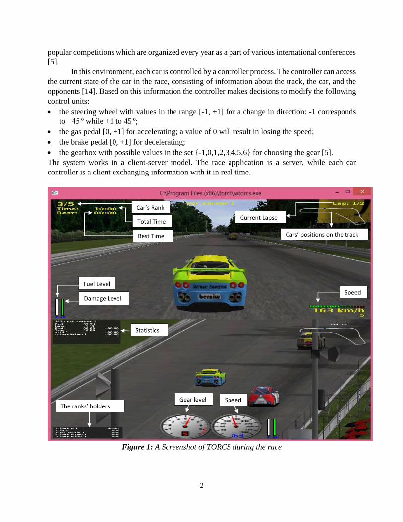
In this environment, each car is controlled by a controller process. The controller can access

the current state of the car in the race, consisting of information about the track, the car, and the

opponents [14]. Based on this information the controller makes decisions to modify the following

control units:

the steering wheel with values in the range [-1, +1] for a change in direction: -1 corresponds

to −45 o while +1 to 45 o;

the gas pedal [0, +1] for accelerating; a value of 0 will result in losing the speed;

the brake pedal [0, +1] for decelerating;

the gearbox with possible values in the set {-1,0,1,2,3,4,5,6} for choosing the gear [5].

The system works in a client-server model. The race application is a server, while each car

controller is a client exchanging information with it in real time.

Figure 1: A Screenshot of TORCS during the race

Car’s Rank

Total Time

Best Time

Fuel Level

Damage Level

Current Lapse

Cars’ positions on the track

Speed

Speed Gear level

Statistics

The ranks’ holders

3

As it is shown in Figure 1, the upper screen of TORCS displays the client and its

information such as the car’s rank, the total time that the car spent from the beginning of the race,

the best time that has been taken to complete a lapse, and other measurements such as the positions

of the cars on the track, the fuel, the damage, and the speed. The lower screen shows the race from

another angle; this screen displays one of the opponent cars if any of them are present. It also

displays the statistics of that car, gear levels, and the speed of the car. It also shows the holders of

the first five ranks.

The remainder of the thesis is organized in the following way. In Chapter 2 we discuss a

few previous papers, works, and other materials that are relevant to our controller. In Chapter 3

we discuss the procedural methods and the learning methods that we have already used and

developed further to improve the driver algorithm that we started from. Chapter 4 discusses the

experimentation methodology that we used to evaluate the controller’s performance.

4

2. Literature Review

The work in this thesis is based on the EPIC controller as presented by Guse and Vrajitoru in [5].

EPIC was submitted to the GECCO 2009 competition [16]. In this competition, cars driven by

code submitted by the competitors run against each other in a race. Beside the car status, the

controllers are provided with information about the angle with the track’s center line, the free

distance ahead within 45 degrees of the car direction, and information about close opponents. The

paper describes a car driver based on two components: determining the target angle for turning in

each frame, and determining the target speed in the next frame. The controller calculates the target

angle based on the target direction in an efficient way. It also provides a sharp turn detecting system

which allows adjusting the target speed for an approaching sharp turn to keep the car inside the

track. The system also adjusts the target angle if it determines that it might lead the car out of the

track [5]. EPIC depends on the principle of calculating the free available distance ahead to

determine the target angle. However, this controller lacks a component to handle opponents, and

the movement along the track requires more fluency. So, we started improving the EPIC code to

achieve these desirable goals.

Many approaches can be found in the literature for track prediction with the purpose of

optimizing the performance. Such predictions help the controller to make early decisions on

adjusting the steering angle and the target speed, in order to keep the car inside the track. Such an

approach allows the controller to minimize the damage to the vehicle and to reduce the time

required to complete the race.

One popular approach of track prediction depends on calculating the distance ahead, such

as the one used in the EPIC controller. It calculates the free available distance ahead of the car to

determine the target angle. Another approach is “the track segmentation”, in which the track is

divided into pieces and these pieces are classified as pre-defined types of polygons. Then the

controller reconstructs a full track model from these polygons, as presented in [15].

Another controller based on the track segmentation principle is presented by Onieva et al.

[13]. Their controller was submitted to TORCS Racing Car Competition 2009 [16]. The

architecture of the controller consists of five simple modules that control gear shifting, steer

movements, and pedals positions [13]. In addition, the target speed is adjusted by the “TSK fuzzy

system”. As the authors pointed out, “Fuzzy rule-based systems are considered one of the most

important applications of the fuzzy set theory suggested by “Zadeh [20]”. When the car is inside

the track, the target speed is calculated based on certain rules [13]. The most important aspect of

this work is the opponent modifier. It controls the driving behavior in situations when an opponent

is nearby by adjusting the steering controller and the braking controller immediately. However,

this approach doesn’t take into consideration the factor of the opponent’s speed. In general, this

paper provides an important contribution for detecting the track mode and handling the opponents

for autonomous cars.

Another paper [14], also written by Onieva et al. in 2012, presents a driving controller

called AUTOPIA for the simulated racing car competition. It provides a full driving architecture

including six separate main tasks: gear control, pedal control, steering control, stuck situation

manager, target speed determination, opponent modifier, and learning module [14]. The

performance of the controller was tested in two efficient ways: it was running over several tracks

with and without opponents. Several measures of performance were reported, such as participating

5

in international competitions and running the car on several tracks once alone and another time

with opponents. The controller was submitted as a participant to the 2010 Simulated Racing car

Competition, in which it won laurels in the end as the authors claimed [14]. The paper provides a

simple and a powerful architecture especially for the opponent modifier. It deals with opponents

in all directions in a simple approach. When an opponent is present within unallowable distances,

heuristic rule sets are applied for pedal control and steering control [14].

Furthermore, many learning approaches are presented to find the optimal path the car

should follow to reduce the time required to complete the race. Finding the optimal path could be

accomplished by shortening the distance covered by the car and avoiding unnecessary turns.

“The evolutionary learning approach” is presented in a paper by Kim, Na et al. [7]. It

presents an optimized algorithm which was used for an autonomous car controller using “self‐adaptive” evolutionary strategies (SAESs) [7]. Kim, Na et al. developed additional rules and

parameters to enhance the performance of their previous model, and they applied new learning

approaches to these rules and parameters [7]. This work is well-experimented and it provides

learning approaches that are able to derive the parameters used to determine the target speed in an

efficient and easy to generalize way. Yet, it lacks an opponent handling system.

Another controller using the evolutionary learning system is presented by Quadflieg et al.

in [15]. The controller is based on the track segmentation principle. It was submitted to TORCS

Racing car Competition 2010 [15]. This controller uses a simple evolutionary learning approach

which enables planning the path ahead for the car [15].

More recently, another learning approach which uses hyper-heuristics in a real-valued

mode in a paper [8] by Kole, M et al. It presents the TORCS-based car system as a real valued

optimization problem and studies the performance of different methodologies including a set of

heuristics and their combination controlled by a selection hyper-heuristic framework. The study

shows that hyper-heuristics perform well in the TORCS environment [8].

Artificial neural networks (ANN) are also used as a learning system. The ANN can be

traced back to 1943 when the neurophysiologist Warren McCulloch and the mathematician Walter

Pitts developed a simple model for an artificial neural network in order to describe how the brain’s

neurons might work. Their artificial neural network was designed using electrical circuits [24].

Five years later, a paper, written by Donald Hebb, pointed out that the neural paths become

stronger every time they are used, which is considered an important principle in the human learning

process [24]. This paper inspired scientists to think that neural networks could learn from examples

in a similar way.

In 1959, the first neural networks applied to a real world problem were called "ADALINE"

and "MADALINE" and were developed by Bernard Widrow and Marcian Hoff from Stanford

[24]. Later, the reputation of neural networks diminished due to the fact that some computer

scientists suggested that there is no productivity for developing such neural networks [24]. This

resulted in a significant elimination of funding and research with artificial neural networks [24].

During the late 1970s and early 1980s, a public interest emerged again in the neural

networks field. In 1982, there was a joint US-Japan conference on Cooperative/Competitive

Neural Networks [24]. Japan unveiled its fifth generation of neural networks, and US academia

were worried that the US could be left behind in the neural networks field. Thus, there was more

funding and more research raised in the field. As a result, within the next four years later, the back-

6

propagation neural networks and the hybrid networks with multiple layers were developed [24].

Currently, their value is recognized by the computer science community and they have a vast

number of applications. They seem especially suited for areas related to control, that our project

belongs to.

In [12], a controller presented by Mun˜oz, et al. was submitted to the 2010 Simulated

Racing car Championship. It is “a human-like controller” using neural networks [12]. It adopts the

principle of track segmentation. The controller builds a model of the tracks using the neural

networks to predict the trajectory the car should follow and the target speed [12]. “The neural

networks are trained with data retrieved from a human player, and are evaluated in a new track”

[12]. The ANNs are trained to reach the optimal path the car should take to behave similarly to the

human player. This work shows a satisfying result of predicting the trajectory in new tracks;

however, the target speed is most likely slower than the human's on the same tracks because of the

absence of an opponent overtaking component, as the authors mentioned [12].

A different controller suggested by Chaudhary and Sharma in [3] generates the optimal

racing line using artificial neural networks. The controller choses the optimal racing line within a

scope angle of 15 degrees that gives the maximum possible speed in every point on the path.

Overall, most of the works succeeded in building either a track prediction system or an

opponent-handling system. It is challenging to deal with opponents while the car is traveling on a

specific target angle and at a specific target speed. Sometimes, the presence of opponent requires

adjusting the steering angle and modifying the speed, either by accelerating or decelerating. Thus,

most of the papers focus on improving track prediction systems regardless of the presence of the

opponents.

On the other hand, there are a few papers discussing the speed prediction, such as [5]. Here,

the Hill Climbing (HC) learning approach was used in EPIC to find the optimal safe speed the car

should take to reduce the damage resulting from miscalculated speed [5]. The HC creates the first

candidate solution and then produces the offspring using “a parameterless search operation”. The

search operation performs a loop in which the optimal solution at the current time is used to

produce one child. If this new child is better than its parent, it replaces it. Then, the cycle starts all

over again [19]. The algorithm does not maintain a search tree: it looks for an appropriate path

only from the current state to immediate future states. Hill Climbing is widely used in networking

and communication, robotics, data mining and data analysis, and developing behaviors for game

players [19].

We will compare our model with both the EPIC controller described earlier in this section,

and with a Simple Driver controller provided by the TORCS engine as part of the client code. The

Simple Driver is a very simple controller providing basic modules for steering control and

accelerating/brake control. It keeps the car in the middle of the track as much as possible, and it

applies a simple recovery policy if the car is stuck.

7

3. Auto Pilot Methods In this chapter, we will discuss in more detail the procedural and learning methods that we used to

improve the EPIC algorithm that this research is based on. In the procedural methods, we will

describe the units that we added to enhance the performance of the Gazelle driver. As part of the

discussion of the learning methods, we will describe some algorithms that we used to improve the

procedural driver automatically.

3.1 Benchmark Pilots

For a valid evaluation of the Gazelle’s performance, we need similar controllers to Gazelle to

compare our various models with them. We chose two pilots that were available to us together

with the source code: the Simple Driver and the EPIC controller.

1. The Simple Driver

This pilot was provided by the TORCS software, and it was developed by Daniele Loiacono in

2007 [10]. It contains very basic functions to control the racing car to give the developers an idea

of what the controller should look like. It contains simple functions to control the gear, steering

angle, and the speed without dealing with opponents. Here are the principles of car driving in this

system.

If the car is found at an angle with the road axis that is greater than 30 degrees for at least

25 consecutive frames, then it is considered to be "stuck". In this case, the simple driver sets the

car in reverse with an angle that is the negative of the current angle with the road. It drives the car

this way at a low speed until the car's front is oriented towards the border of the road. For example,

if the car is on the left side, then it should be facing left. At that point, the car is shifted into first

gear and the steering angle is reversed, so that the car can start moving forward again. Both the

EPIC driver and the Gazelle are using this algorithm to deal with stuck situations.

If the car is not stuck, then the Simple driver proceeds the following way:

First, it computes the target speed. For this, it gets the distance ahead along the car's axis from the

sensors (labeled cSensor), then at 5 degrees to the left (lSensor), and at 5 degrees to the right

(rSensor), as shown in Figure 2. Let's assume that rSensor > cSensor. Then the driver first makes

an estimation of the "turnAngle" which is the angle between the tangent to the road in the point

that the car is oriented towards and the direction of movement plus 5 degrees. If lSensor < cSensor,

the angle is taken based on the direction of movement minus 5 degrees. Then the target speed is

computed as:

targetSpeed = [maxSpeed * cSensor * sin(turnAngle) ] / maxSpeedDist

where:

maxSpeed = 150km/h and maxSpeedDist = 70 m.

8

Figure 2: Determining the speed in the Simple Driver

Second, it computes the target angle for steering the car by simply aiming to keep the car

parallel to the track axis and close to the center of the road. At high speed, this driver reduces the

steering command to avoid loosing control of the car.

In addition to these, the Simple Driver also provides some functions for changing the gear

and for converting a target angle or speed into the correct value for the steering and acceleration.

These were used both EPIC and Gazelle.

2. EPIC

This autonomous driver that was used as a starting point for writing Gazelle, and was developed

by Dana Vrajitoru and Charles Guse [5]. EPIC was submitted to the GECCO 2009 competition

[16]. This pilot has the next properties:

The general algorithm of EPIC consists in the following steps:

calculate the target direction and speed,

determine the correct gear,

calculate the target angle based on the target direction,

calculate the acceleration and the brake based on the target angle and speed [5].

First, for the target direction, EPIC starts by deciding if the car can continue to travel in the

current direction. The conditions for persisting in the same direction are:

if the current direction of the car is close enough to the direction of the road centerline,

if there is enough free distance straight ahead in the car’s direction of movement,

if the car is safely inside the track[5].

If the previous conditions are not met, and the car is too close to the border of the road or

if it is outside the road altogether, then EPIC has to take a new direction by modifying the steering

angle to get closer to the road centerline[5].

Second, the target speed is computed. Thus, the speed at which the car can safely ride

depends on how straight it is going. The safe conditions for the speed are considered to be:

if the car is going almost straight,

9

if the free distance in front of the car in the new direction set by the target angle is large enough,

if no sharp turn is anticipated to follow up on the road soon[5].

If the three conditions above are met, then the speeding up is set to its maximal value. This

situation is called pedal to the metal [5]. In any other case, a large value for the target speed is set

to start with, which is first scaled by the sine of the target angle for steering the angle and with the

available free distance in the target direction [5].

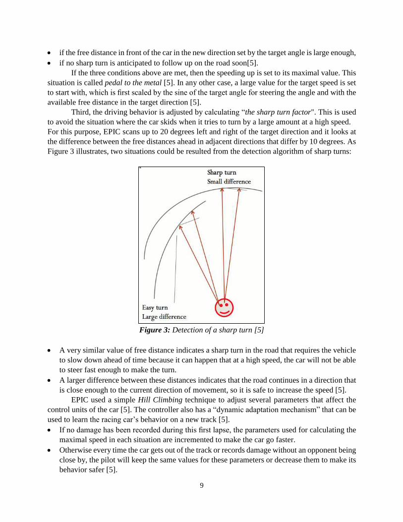
Third, the driving behavior is adjusted by calculating “the sharp turn factor". This is used

to avoid the situation where the car skids when it tries to turn by a large amount at a high speed.

For this purpose, EPIC scans up to 20 degrees left and right of the target direction and it looks at

the difference between the free distances ahead in adjacent directions that differ by 10 degrees. As

Figure 3 illustrates, two situations could be resulted from the detection algorithm of sharp turns:

Figure 3: Detection of a sharp turn [5]

A very similar value of free distance indicates a sharp turn in the road that requires the vehicle

to slow down ahead of time because it can happen that at a high speed, the car will not be able

to steer fast enough to make the turn.

A larger difference between these distances indicates that the road continues in a direction that

is close enough to the current direction of movement, so it is safe to increase the speed [5].

EPIC used a simple Hill Climbing technique to adjust several parameters that affect the

control units of the car [5]. The controller also has a “dynamic adaptation mechanism” that can be

used to learn the racing car’s behavior on a new track [5].

If no damage has been recorded during this first lapse, the parameters used for calculating the

maximal speed in each situation are incremented to make the car go faster.

Otherwise every time the car gets out of the track or records damage without an opponent being

close by, the pilot will keep the same values for these parameters or decrease them to make its

behavior safer [5].

10

EPIC has several well-developed functions, however, it required some improvements such

as:

Making the pilot react to any approaching opponent as EPIC couldn’t handle the opponents.

The racing car sometimes is swinging while it is traveling on the road. Such instable movement

needs to be improved to make the car’s movement more balanced.

3.2 Procedural Methods

The TORCS engine provides the following information to the controllers: a car status containing

the current speed, the angle with the centerline of the road, the distance from the center of the road,

and more; an array of sensors detecting the distance to the road border in a 5 degrees increment in

a range of [-45, 45] degrees around the car's direction of movement; and array of opponent sensors

with information about opponents present within a 200m radius of the car in all directions.

The first goal of this thesis was to implement the Gazelle controller efficiently by

improving the existing modules from the EPIC controller and by adding new components to deal

with aspects not present in the EPIC driver. The EPIC driver is the starting module for the Gazelle

driver. We also added new modules to deal with opponents and reduce the damage caused by

hitting the hard shoulders of the road.

The Gazelle Controller

The Gazelle controller consists of three components: the target direction unit, the target speed unit,

and the opponent adjuster. The target direction unit controls the direction in which the car is

moving. The target speed unit adjusts the speed based on the target direction, while the Opponent

Adjuster adjusts the direction and speed based on the opponents’ presence. Below we will describe

each unit in more detail.

Target Direction Unit

The unit determines the target angle using the following guidelines:

If the current direction of the car is close enough to the road centerline, there is enough distance

straight ahead, and the car is safely inside the track, then the car can continue in the same

direction.

Otherwise, we start with the direction of the road centerline, and scan by 10 degrees in the

direction in which the distance ahead increases, until we find an angle at which it decreases, or

we reach the maximal turn angle of 45o. Figure 4 (source: [5]) shows this scanning process of

searching for a good path of movement.

11

Figure 4: The scanning process [5]

If the car is too close to the border of the road or gets outside, we add a direction change to

move it back inside. Currently, the borders threshold, denoted by safelyInsideTrack, is at 85%

distance from the center of the road, to account for the width of the car. Let trackPosition be

the current position of the car on the road, taking values between -1 and 1. If

abs(trackPosition)>safeInsideTrack, then the new target angle is computed as:

−25 ∗ sign(𝑡𝑟𝑎𝑐𝑘𝑃𝑜𝑠𝑖𝑡𝑖𝑜𝑛)(abs(𝑡𝑟𝑎𝑐𝑘𝑃𝑜𝑠𝑖𝑡𝑖𝑜𝑛) − 𝑠𝑎𝑓𝑒𝑙𝑦𝐼𝑛𝑠𝑖𝑑𝑒𝑇𝑟𝑎𝑐𝑘)

Where the function abs returns the absolute value of a number and the function sign returns -1

for a negative number, 0 for 0, and 1 for a positive number. This formula scales 25 degrees by

how far the car is from the threshold. If the computed target angle already has a value of the

same sign but of a larger absolute value, then this new target angle is not used because the

normal method is performing the adjustment already.

If the current turning angle is good enough, we maintain it for movement continuity. This is

determined by comparing the free distance ahead with the free distance 10 degrees left and

right; if the distance ahead is the largest of the three values, then we can maintain the current

angle. This is an addition to the Gazelle controller to improve the fluency of the car’s

movement.

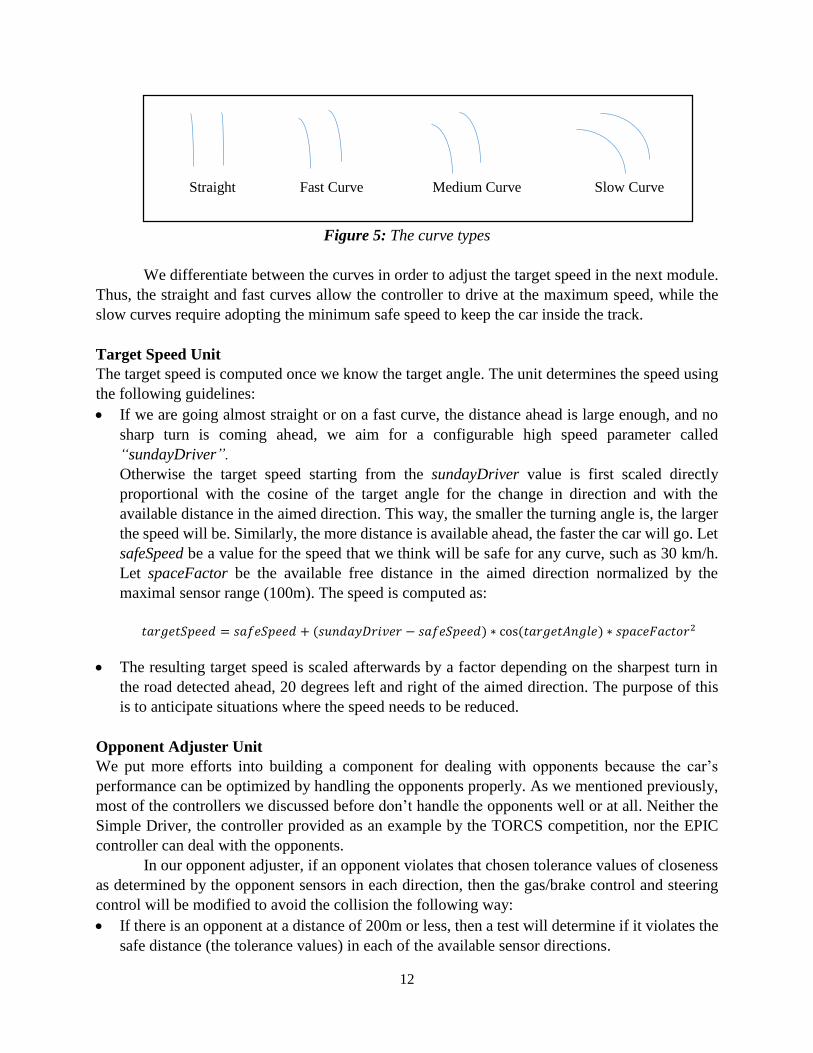
As Figure 5 shows, after the target angle is computed, we identify four types of situations

on the road:

Straight: if the road is straight ahead of the car and the target angle is between 0o and 10o.

Fast Curve: if the upcoming curve is small enough and its angle is between 10o and 15o.

Medium Curve: if the angle of the upcoming curve is between 15o and 30o.

Slow Curve: if the upcoming curve is wide and the target angle is greater than 30o.

12

Figure 5: The curve types

We differentiate between the curves in order to adjust the target speed in the next module.

Thus, the straight and fast curves allow the controller to drive at the maximum speed, while the

slow curves require adopting the minimum safe speed to keep the car inside the track.

Target Speed Unit

The target speed is computed once we know the target angle. The unit determines the speed using

the following guidelines:

If we are going almost straight or on a fast curve, the distance ahead is large enough, and no

sharp turn is coming ahead, we aim for a configurable high speed parameter called

“sundayDriver”.

Otherwise the target speed starting from the sundayDriver value is first scaled directly

proportional with the cosine of the target angle for the change in direction and with the

available distance in the aimed direction. This way, the smaller the turning angle is, the larger

the speed will be. Similarly, the more distance is available ahead, the faster the car will go. Let

safeSpeed be a value for the speed that we think will be safe for any curve, such as 30 km/h.

Let spaceFactor be the available free distance in the aimed direction normalized by the

maximal sensor range (100m). The speed is computed as:

𝑡𝑎𝑟𝑔𝑒𝑡𝑆𝑝𝑒𝑒𝑑 = 𝑠𝑎𝑓𝑒𝑆𝑝𝑒𝑒𝑑 + (𝑠𝑢𝑛𝑑𝑎𝑦𝐷𝑟𝑖𝑣𝑒𝑟 − 𝑠𝑎𝑓𝑒𝑆𝑝𝑒𝑒𝑑) ∗ cos(𝑡𝑎𝑟𝑔𝑒𝑡𝐴𝑛𝑔𝑙𝑒) ∗ 𝑠𝑝𝑎𝑐𝑒𝐹𝑎𝑐𝑡𝑜𝑟2

The resulting target speed is scaled afterwards by a factor depending on the sharpest turn in

the road detected ahead, 20 degrees left and right of the aimed direction. The purpose of this

is to anticipate situations where the speed needs to be reduced.

Opponent Adjuster Unit

We put more efforts into building a component for dealing with opponents because the car’s

performance can be optimized by handling the opponents properly. As we mentioned previously,

most of the controllers we discussed before don’t handle the opponents well or at all. Neither the

Simple Driver, the controller provided as an example by the TORCS competition, nor the EPIC

controller can deal with the opponents.

In our opponent adjuster, if an opponent violates that chosen tolerance values of closeness

as determined by the opponent sensors in each direction, then the gas/brake control and steering

control will be modified to avoid the collision the following way:

If there is an opponent at a distance of 200m or less, then a test will determine if it violates the

safe distance (the tolerance values) in each of the available sensor directions.

Straight Fast Curve Medium Curve Slow Curve

13

If there is an opponent in the front of the car, on the sides, or in the rear of the car within an

unallowable space, the following flags are turned on, causing a reaction of the respective

modules:

• A Brake flag for an opponent in the front. This flag takes care of the sensors in the range

of -40o to 40o [13]. If an opponent is found within an unallowable space and its speed is

close to ours, the car should brake immediately by modifying the brake/accelerate value to

the half of the current speed. The tolerance values are shown in Table 1 and were adopted

from [13].

Table 1: Opponents adjuster over the gas & brake action [13]

Orientation of the Opponent Sensor Tolerance Value

±40o 6 m

±30o 6.5 m

±20o 7 m

±10o 7.5 m

0 o 8 m

• A Steering flag for an opponent in the front or on the side, it takes care of the opponent

sensors in the range of -100o to 100o, also adopted from [13]. An overtaking manoeuver

requires to modify the steering angle if the opponent violates the tolerance values. The

tolerance values are shown in Table 2.

Table 2: Opponent sensors tolerances for overtaking [13]

Orientation of the Opponent Sensor Tolerance Value

0o, ±10o 20 m

±20o 18 m

±30o 16 m

±40o 14 m

±50o 12 m

> ±50o 10 m

• An Accelerating flag for an opponent at the rear of the car driving at an equal or higher

speed than ours. Increments values are summarized in Table 3.

Table 3: Opponent sensors increments for overtaking [13]

Orientation of the Opponent Sensor Increment Value

0o, ±10o ±0.20o

±20o ±0.18o

±30o ±0.16o

±40o ±0.14o

±50o ±0.12o

> ±50o ±0.10o

14

Trouble Spots Register

This component was added in order to avoid the accidents caused by mistakes in predicting the

right steering angle, leading the car out of the track. In TORCS competitions, the race starts with

a warming level which allows drivers to learn the track. After that the actual race takes place in

the second level. Thus, we introduced the “Trouble Spots Register” detecting and storing places

in the track where the car gets out of the road starting from the warming level. In the subsequent

lapses of the circuit, to avoid repeating these mistakes, we use a method decelerating the speed

whenever the car is close to a trouble spot, by an amount inversely proportional to the distance to

the trouble spot.

A list of "trouble spots" on the road will be stored by the Gazelle driver in a persistent

memory space in order to be accessible at later points during the race. To achieve this, the last

position of the car on the road is stored in each frame. Then when the code detects that the car got

out of the road, this position is added to the list.

In each frame, the current position of the car is compared to the trouble spots. If we are

close enough to one of them, the speed will be adjusted as mentioned above. The closer we are to

the trouble spot, the faster the car will decelerate.

The issue arises from the fact that the visibility of the driver is limited to 100m ahead and

that it is difficult to break down the speed fast enough if the situation requires it. For this reason

we adopted the approach of detecting a sharp turn on a road combined with the trouble spots

detector.

3.3 Learning Methods Overview

In this part of the research, we aimed to optimize the performance of the procedural driver

automatically using learning methods. Even though the ANN is initially not expected to

outperform the original function that it learns from, which is the procedural Gazelle in our case, it

has the potential to continue learning afterwards from real-time observations and become better

over time. Also, we can expect some amount of noise in the procedural heuristics that can be

reduced by the use of an ANN, and the pilot’s performance can be improved as a result. As we

mentioned before, our goal was to minimize the damage as much as possible, and to reach the

maximum safe speed. These two goals can be achieved by reaching the ideal target angle and the

ideal target speed. We need to enable the controller to learn before and during the race using

learning algorithms. We will use two main algorithms for this purpose: Artificial Neural Networks

and Hill Climbing.

An Artificial Neural Network (ANN) is a learning method that is inspired by the way the

human’s biological nervous system processes information. Such a system is composed of a large

number of connected neurons, the processing elements, in which components work together to

solve a specific problem [22]. The ANN is a “layered structure” consisting of three main layers:

the inputs layer, the hidden layer, and the outputs layer [9]. The hidden layer uses the learning

processing elements (neurons) to adjust the input values combined with a set of parameters in order

to produce the optimal output solution.

ANNs can learn by examples and they can be used for pattern recognition or data

classification, and they are also appropriate for prediction or forecasting [22]. There are many

applications of ANNs such as modeling and diagnosing the cardiovascular system, sales

15

forecasting, industrial process control, customer research, data validation, risk management, target

marketing, and credit evaluation [22].

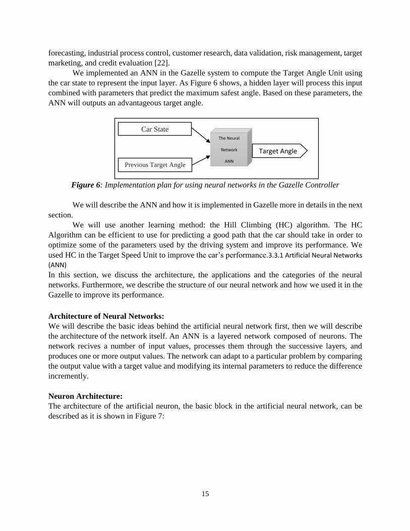
We implemented an ANN in the Gazelle system to compute the Target Angle Unit using

the car state to represent the input layer. As Figure 6 shows, a hidden layer will process this input

combined with parameters that predict the maximum safest angle. Based on these parameters, the

ANN will outputs an advantageous target angle.

Figure 6: Implementation plan for using neural networks in the Gazelle Controller

We will describe the ANN and how it is implemented in Gazelle more in details in the next

section.

We will use another learning method: the Hill Climbing (HC) algorithm. The HC

Algorithm can be efficient to use for predicting a good path that the car should take in order to

optimize some of the parameters used by the driving system and improve its performance. We

used HC in the Target Speed Unit to improve the car’s performance.3.3.1 Artificial Neural Networks

(ANN)

In this section, we discuss the architecture, the applications and the categories of the neural

networks. Furthermore, we describe the structure of our neural network and how we used it in the

Gazelle to improve its performance.

Architecture of Neural Networks:

We will describe the basic ideas behind the artificial neural network first, then we will describe

the architecture of the network itself. An ANN is a layered network composed of neurons. The

network recives a number of input values, processes them through the successive layers, and

produces one or more output values. The network can adapt to a particular problem by comparing

the output value with a target value and modifying its internal parameters to reduce the difference

incremently.

Neuron Architecture:

The architecture of the artificial neuron, the basic block in the artificial neural network, can be

described as it is shown in Figure 7:

Car State

Previous Target Angle

The Neural

Network

ANN

Target Angle

16

Figure 7: The basic of artificial neuron [1]

Figure 7 shows that various inputs to the neuron are represented by 𝑥(𝑖). Each of these

inputs is multiplied by a connection weight 𝑤(𝑖). These products are summed, fed through a

transfer function to generate a result, which is returned as the output [1]. The transfer function or

the activation function is the formula that defines the outputs of a neuron using an input or set of

inputs. The activation function that we used is the hyperbolic tangent of the sum of weighted

inputs, which is a classic function for neural networks taking values in the interval [-1, 1]:

𝑂𝑢𝑡𝑝𝑢𝑡 = tanh (∑( 𝑤(𝑖)𝑥(𝑖))

𝑛

𝑖=0

)

Since the output of the network in our case is an angle in radians limited to the range [-45º,

45º], we do not need to scale the output of the neuron.

Network Architecture:

As it is shown in Figure 8, the network consists of three layers:

Input layer: consists of neurons representing external input data which play a role in

characterizing the output.

Hidden layers: The architecture of these layers is characterized by the number of layers

and the number of hidden neurons. It contains one or more layers and each layer is

composed of a group of hidden neurons sharing the same inputs [9]. Such layers can do

some basic pattern recognition operations [21].

Output layer: yields the outputs from the neural network.

17

Figure 8: A simple artificial network with three layers (input layer, a hidden layer, and output

layer)

Hidden layer:

We need to consider two concerns related to the hidden layer:

How many hidden layers should we use?

How many hidden neurons should we use?

First: the appropriate number of hidden layers

The number of hidden layers depends on the number of output neurons and on the type of

the activation function. Even if this relationship cannot be established precisely, some

recommendations for appropriate values can be found in the literature [17], [24].

If we have only one input, then there is no need to use more than one hidden layer.

However, an ANN with two or more inputs requires adding another hidden layer [25]. We should

not use any hidden layer if the ANN is a liner model [11]. This does not apply to us since our

activation function is not linear.

If the ANN requires continuous nonlinear hidden-layer activation functions, then one

hidden layer is necessary for the “universal approximation” property [6].

In special architectures such as cascade correction, using more than two hidden layers can

be beneficial [4]. Based on the various indications and recommendations we found, we decided to

use two hidden layers.

Second: the appropriate number of hidden neurons

Many approaches offer "rules of thumb" for choosing the number of the hidden neurons. One

approach suggests that the number of hidden neurons should be between the number of the input

neurons and the number of output neurons [2]. Another approach suggested the maximum number

of hidden neurons should never exceed the double number of the input neurons [18].

In fact, the best number of hidden units shouldn’t depend only on the numbers of input and

output units; indeed, it should take into consideration other aspects such as: the number of training

cases, the amount of noise in the targets, the complexity of the function or classification to be

Input Layer Hidden Layer Output Layer

18

learned, the architecture of the network, the type of hidden unit activation function, and the training

algorithm [25].

In most situations, there is no way to determine the number of neurons in the hidden layer

without trial and error. If we have too few hidden neurons then we will experience a high training

error and if we have too many hidden neurons then we could have a high generalization error

caused by over-fitting [25].

Neural networks applications:

Neural networks are applicable to many real world problems. As neural networks are successful

in identifying patterns in given data, they are well appropriate for prediction and forecasting such

as: sales forecasting, industrial process control, customer research, data validation, risk

management, target marketing, credit evaluation, diagnosing diseases, and suggesting treatment

[24].

Neural networks categories:

There are two main categories of the network architectures:

1. Feed-forward networks: allow the input data to travel one way only; from the input layer

to the output layer. In fact, the output of any layer doesn’t affect that same layer since there

are no feedback operations [24]. In this way, in a feed-forward neural network, “the output

of each neuron is a function of the inputs” as following:

Output= f (inputs) [9].

2. Feed-backward networks: allow traveling data in both ways, forward and backward. Such

a network keeps adjusting connections’ weights until it reaches a balanced state where the

error between the desirable output and the actual output is diminished [24]. We used a feed-

backward ANN in the Gazelle system.

3.4 The Neural Network Used in Gazelle

We used a neural network within the Gazelle system to determine the target angle and we designed

the architecture of the neural network as follows:

Output layer: Derives the target angle that can be taken in the next frame.

• The count of the output neurons is 1 or 5, as we shall explain later.

Input layer: We need a set of 5 parameters as input data for the neural network. As shown in

Figure 9, these inputs include the car state and the track properties as following:

19

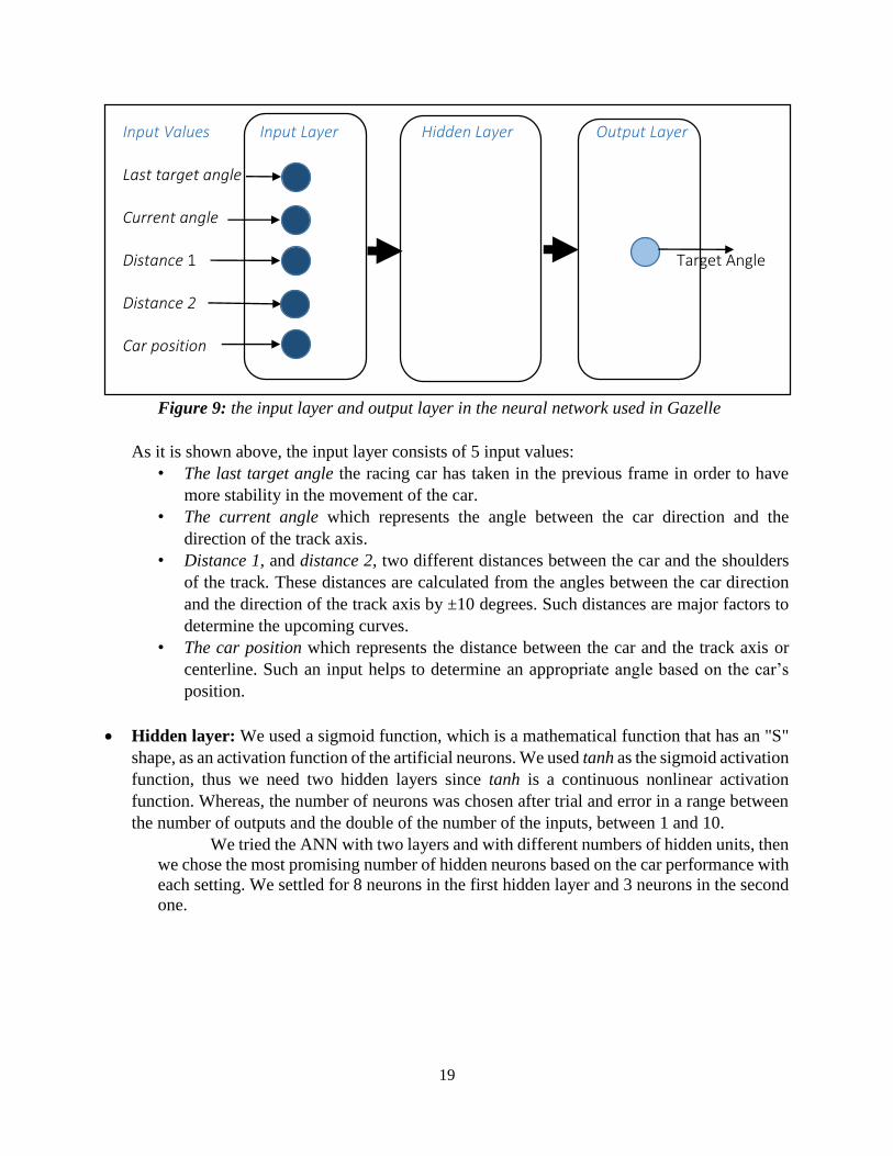
Figure 9: the input layer and output layer in the neural network used in Gazelle

As it is shown above, the input layer consists of 5 input values:

• The last target angle the racing car has taken in the previous frame in order to have

more stability in the movement of the car.

• The current angle which represents the angle between the car direction and the

direction of the track axis.

• Distance 1, and distance 2, two different distances between the car and the shoulders

of the track. These distances are calculated from the angles between the car direction

and the direction of the track axis by ±10 degrees. Such distances are major factors to

determine the upcoming curves.

• The car position which represents the distance between the car and the track axis or

centerline. Such an input helps to determine an appropriate angle based on the car’s

position.

Hidden layer: We used a sigmoid function, which is a mathematical function that has an "S"

shape, as an activation function of the artificial neurons. We used tanh as the sigmoid activation

function, thus we need two hidden layers since tanh is a continuous nonlinear activation

function. Whereas, the number of neurons was chosen after trial and error in a range between

the number of outputs and the double of the number of the inputs, between 1 and 10.

We tried the ANN with two layers and with different numbers of hidden units, then

we chose the most promising number of hidden neurons based on the car performance with

each setting. We settled for 8 neurons in the first hidden layer and 3 neurons in the second

one.

Input Values Input Layer Hidden Layer Output Layer

Last target angle

Current angle

Distance 1 Target Angle

Distance 2

Car position

20

Figure 10: the car’s performance differs based on the count of the hidden neurons

As it is shown in Figure 10,

If the neurons of the first layer are less than 7, then the car curves to the right

If the neurons of the first layer are more than 9, then the car curves to the left.

If the neurons of the first layer are 7 or 9 , then the car swings between the shoulders of the

track.

If the neurons of the first layer are 8, then the car travels in the middle of the trak in a stable

behavior.

Then the best performance of the car happened when the count of the neurons for the first

hidden layer was 8.

We chose 8 neurons for the first hidden layer, then we applied the same procedure

to choose the appropiate number for the second hidden layer. We found out that 3 neurons in the

second hidden layer made the car perform in a balanced way travelling in the middle of the track.

To summarize,

The count of the neurons for the first hidden layer =8

The count of the neurons for the second hidden layer =3

… . 6 7 8 9 10 …

Neurons count in the first hidden layer

21

NN implementation

We intended for the ANN to be trained many times with each data set to get the best weights that

can make the racing car perform well. We used a “classic back-propagation model” within an ANN

system that was developed by Dave Miller [26]. This model comes with a video tutorial that is

presented as a guideline for the programmers to design, analyze, and implement a neural network

[26].

Starting from the existing code for the ANN and Gazelle, we edited it to include advanced

tasks such as:

Output the training data to an external text file during the race when the ANN is disabled for

the purpose of collecting the training data.

Read the training data file when the client is running and the ANN is enabled.

Assign the number of iterations that the ANN needs to be trained with, during the training

process.

Output the error rate, during the training process, to be analyzed later.

Enable to choose between Best-weights model and Last-weights model:

• The Best-weights model keeps the best values of the weights when the ANN presented the

minimum average error during the training process.

• The Last-weights model keeps the latest values of the weights acquired at the end of the

training process.

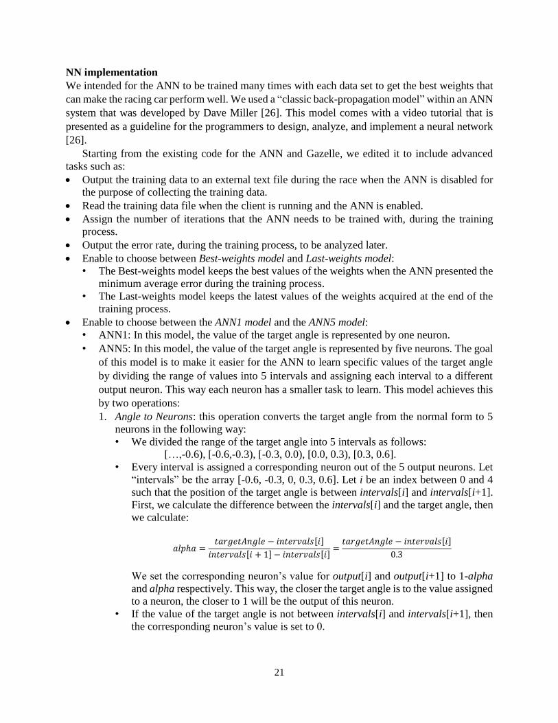
Enable to choose between the ANN1 model and the ANN5 model:

• ANN1: In this model, the value of the target angle is represented by one neuron.

• ANN5: In this model, the value of the target angle is represented by five neurons. The goal

of this model is to make it easier for the ANN to learn specific values of the target angle

by dividing the range of values into 5 intervals and assigning each interval to a different

output neuron. This way each neuron has a smaller task to learn. This model achieves this

by two operations:

1. Angle to Neurons: this operation converts the target angle from the normal form to 5

neurons in the following way:

• We divided the range of the target angle into 5 intervals as follows:

[…,-0.6), [-0.6,-0.3), [-0.3, 0.0), [0.0, 0.3), [0.3, 0.6].

• Every interval is assigned a corresponding neuron out of the 5 output neurons. Let

“intervals” be the array [-0.6, -0.3, 0, 0.3, 0.6]. Let i be an index between 0 and 4

such that the position of the target angle is between intervals[i] and intervals[i+1].

First, we calculate the difference between the intervals[i] and the target angle, then

we calculate:

𝑎𝑙𝑝ℎ𝑎 =𝑡𝑎𝑟𝑔𝑒𝑡𝐴𝑛𝑔𝑙𝑒 − 𝑖𝑛𝑡𝑒𝑟𝑣𝑎𝑙𝑠[𝑖]

𝑖𝑛𝑡𝑒𝑟𝑣𝑎𝑙𝑠[𝑖 + 1] − 𝑖𝑛𝑡𝑒𝑟𝑣𝑎𝑙𝑠[𝑖]=

𝑡𝑎𝑟𝑔𝑒𝑡𝐴𝑛𝑔𝑙𝑒 − 𝑖𝑛𝑡𝑒𝑟𝑣𝑎𝑙𝑠[𝑖]

0.3

We set the corresponding neuron’s value for output[i] and output[i+1] to 1-alpha

and alpha respectively. This way, the closer the target angle is to the value assigned

to a neuron, the closer to 1 will be the output of this neuron.

• If the value of the target angle is not between intervals[i] and intervals[i+1], then

the corresponding neuron’s value is set to 0.

22

2. Neurons to angle: in this operation, we retrieve the target angle in its normal form from

the 5 neurons as follows:

• We multiply each value of intervals[i] by the value of the corresponding neuron.

• The resulted products are summed to acquire the target angle in the normal form.

3.5 Dynamic Training

In this section we present another learning component that we added to the ANN to enable it to be

trained in real time during the race. We enhanced the ANN with the Dynamic Training feature that

we developed with the purpose of training the neural network in real time by adjusting its weights

if the target angle is misestimated.

The dynamic system is based on detecting three types of situations:

when the car gets out of the track,

when the car is about to get out of the track,

when the car is stuck.

For each of them, a flag is being raised in the system that can be detected by the dynamic

learning system.

The flag for the car being out of the track is raised when the position of the center of the

car on the road is at more than 85% of the road's width. This is an empirical value established to

account for the width of the car. The flag for the car being stuck is turned on when the angle

between the car axis and the road is at more than 20º. The flag for the car being about to get out of

the track is turned on when the car's position on the road is at more than 80% and the front of the

car is pointing towards the outside of the track.

If either of these flags is turned on, the input values for the neurons (track position, last car

angle with the road, and so on) are fed into the ANN. Then the new target value for the output (the

angle) is adjusted the following way. If the car is already outside of the road, and it had been

pointing out, then the angle is reduced by 10%. If the car had been pointing towards the inside of

the road, it means that it was already trying to correct the trajectory, but the effort was not enough,

so the angle is increased by 10%.

For the flags indicating that the car is about to get out, or to get stuck, if the car was pointing

towards the outside of the road, then the target angle will be multiplied by a factor of –0.25, to

reverse direction and continue the other way by a smaller amount. Otherwise the angle is reduced

by 25%.

Finally, the new target angle is fed to the ANN as the target output, and back-propagation

is used to train the ANN with this new value. We only use one iteration in this case to avoid over-

specializing the network.

3.6 Hill Climbing (HC)

We also present another learning system that enables the controller to adjust its speed during the

race. We used a simple Hill Climbing technique to adjust several parameters that controlled the

car [5]. The Hill Climbing “is simply a loop that continually moves in the direction of increasing

value” and “It terminates when it reaches a ‘peak’ where no neighbor has a higher value” as Stuart

Russell and Peter Norvig state in [17]. Hill Climbing does not look forward beyond the close

neighbors of the current state [17]. This algorithm, which was used earlier by EPIC, has a “dynamic

adaptation mechanism” to learn the behavior of the racing car on a new track [5]. The method

works as follows:

23

If no damage has been recorded during the first lapse, the parameters designating the maximal

speed in each situation are increased to make the car go faster.

Otherwise every time the car gets out of the track or records damage without an opponent being

close by, the pilot will decrease these parameters to make its behavior safer [5].

3.7 Gazelle Contributions

Here is a summary of the improvements on the EPIC system that were made in the Gazelle system:

1. The Opponent Adjuster Unit: a component that enables the Gazelle pilot to deal with

opponents. It reacts to any approaching opponent based on its location and how close it is

to the pilot.

2. Trouble Spots Register: this component is used to discover the areas in which the car gets

out during the first lapse and then to adjust the car’s speed when it is approaching these

areas.

3. Adding an artificial neural network to compute the appropriate target angle precisely. Such

a learning component improves the fluency of the car’s movement.

4. Adding the “Dynamic Training” feature which enables the driver to continue training the

ANN in real time during the race and can potentially help the car to deal more easily with

new tracks.

5. Using the “Hill Climbing” algorithm to adjust the speed during the race to minimize the

damage.

24

4. Experimentation In this chapter, we present all the experimentations that we performed in order to measure the

performance of the Gazelle controller after developing many functions and adding many features.

We start by describing the methodology that we used to measure the performance of the Gazelle.

Then we present the experimental results of running the Gazelle alone, with opponents, and with

using the learning methods.

4.1 Methodology

We established a set of tests to measure the performance of the Gazelle controller comparing it to

previous work. We compared the newly developed methods with two existing controllers: EPIC

and the Simple Driver. We run each controller by chosing the car called “SRC-server1”, which

represents the running client for the tested controller, to compete itself and measure its

performance.

For the tracks, TORCS provides various tracks to choose from. These tracks are designed

by different developers with the purpose of testing the performance of the controller on circuits of

various difficulty and on various types of roads. During the competitions, drivers can expect to be

exposed to unfamiliar roads to challenge their ability to win the race with minimal damage in a

record time. We started by choosing a number of tracks to test the systems on, and by determining

the experimental conditions to be applied to all of them.

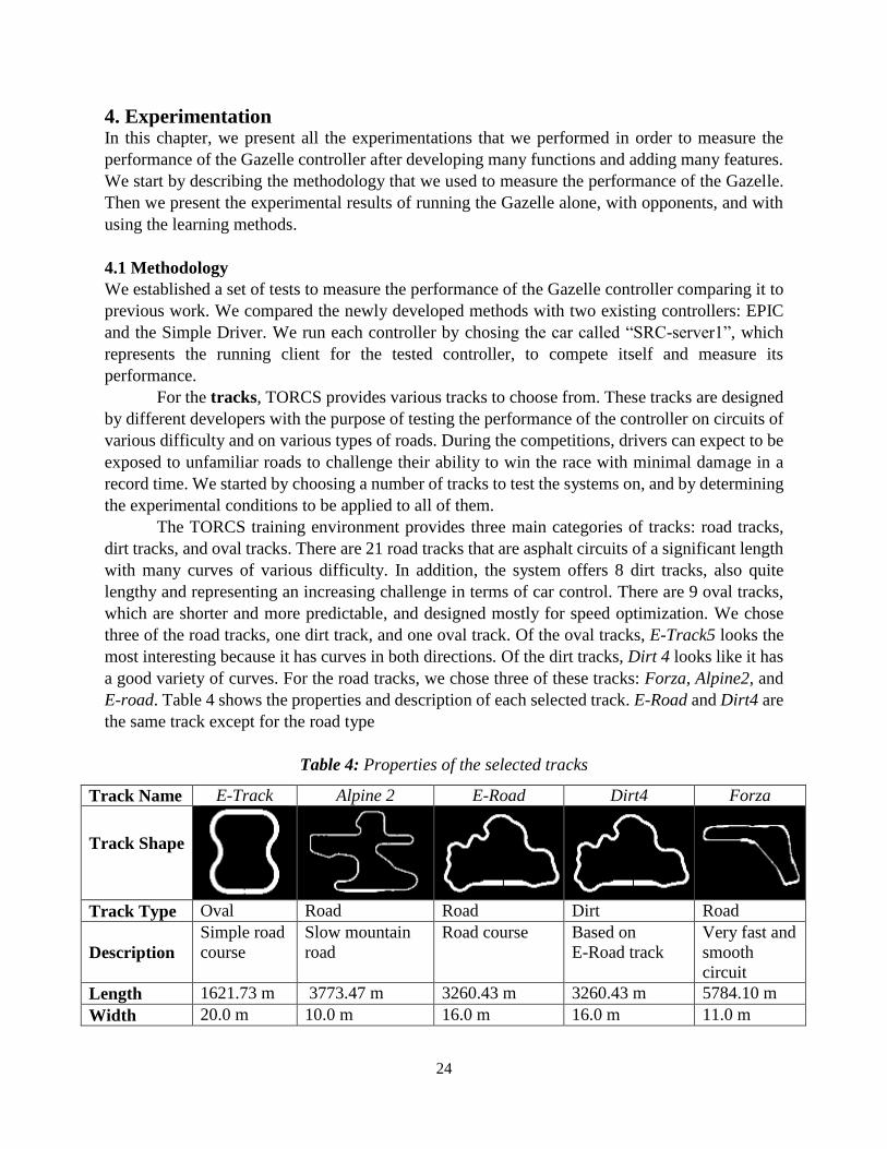
The TORCS training environment provides three main categories of tracks: road tracks,

dirt tracks, and oval tracks. There are 21 road tracks that are asphalt circuits of a significant length

with many curves of various difficulty. In addition, the system offers 8 dirt tracks, also quite

lengthy and representing an increasing challenge in terms of car control. There are 9 oval tracks,

which are shorter and more predictable, and designed mostly for speed optimization. We chose

three of the road tracks, one dirt track, and one oval track. Of the oval tracks, E-Track5 looks the

most interesting because it has curves in both directions. Of the dirt tracks, Dirt 4 looks like it has

a good variety of curves. For the road tracks, we chose three of these tracks: Forza, Alpine2, and

E-road. Table 4 shows the properties and description of each selected track. E-Road and Dirt4 are

the same track except for the road type

Table 4: Properties of the selected tracks

Track Name E-Track Alpine 2 E-Road Dirt4 Forza

Track Shape

Track Type Oval Road Road Dirt Road

Description

Simple road

course

Slow mountain

road

Road course Based on

E-Road track

Very fast and

smooth

circuit

Length 1621.73 m 3773.47 m 3260.43 m 3260.43 m 5784.10 m

Width 20.0 m 10.0 m 16.0 m 16.0 m 11.0 m

25

Figure 11: The Alpine2 track on the left, and the car is travelling on the same track on the right

As Figure 11 shows, the Alpine 2 track is a road track; its shape has many curves of all

kinds: fast, medium and slow curves. Such a road enables us to test the performance more

efficiently. This figure also showcases the material of the road on the right, which looks like

asphalt. Cars in the simulation in TORCS interact with the road’s material and the behavior on the

road depends on it. On Tracks made of asphalt allow the cars to travel more fluently than on a dirt

road.

For each set of experiments, we set the maximum speed and the safe speed for all of the

three drivers with the same value. The maximum speed can vary based on the presence of

opponents and of the neural netork. We shall specify the speed setting for each set of the

experiments. We set the number of lapses on each track to two in all the cases. As the tracks are

generally lengthy, two lapses are enough for an accurate comparison. The second lapse is important

for any driver system that learns some information during the first lapse and it allows us to see if

the learning process is efficient. At the end of the two lapses, the program itself outputs some

information, such as the total time and the damage. We will also add some other measures that

are good indicators of performance: the number of times the car gets out of the road, the total

number of times the car exited the road, and the total distance covered by the end of the race. The

more distance is covered in one lapse, the less efficient the driver is.

Then we will run the three drivers, Simple, EPIC, and Gazelle, on the five tracks and store

these measures for all of them.

4.2 Procedural Gazelle Experiments

We performed a set of experiments to measure the Gazelle performance compared to the

performance of EPIC and the Simple Driver. We set the maximum speed for all the three drivers

to 150 km/h and the safe speed to 100 km/h, and we set the number of lapses to 2 lapses per race.

For this set of experiments, we ran every controller on its own (without opponents) by

running each of them on the five tracks. This means that we needed to run the client 15 times (3

drivers * 5 tracks) to get the results shown in Table 5.

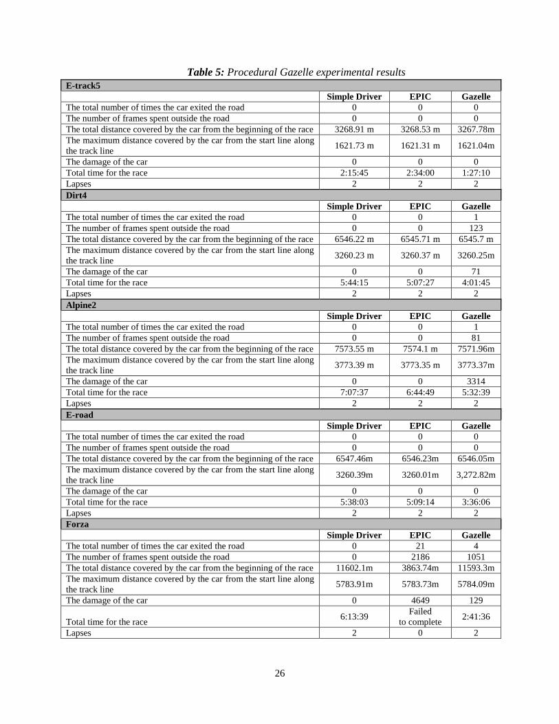
26

Table 5: Procedural Gazelle experimental results

E-track5

Simple Driver EPIC Gazelle

The total number of times the car exited the road 0 0 0

The number of frames spent outside the road 0 0 0

The total distance covered by the car from the beginning of the race 3268.91 m 3268.53 m 3267.78m

The maximum distance covered by the car from the start line along

the track line 1621.73 m 1621.31 m 1621.04m

The damage of the car 0 0 0

Total time for the race 2:15:45 2:34:00 1:27:10

Lapses 2 2 2

Dirt4




The total distance covered by the car from the beginning of the race 6546.22 m 6545.71 m 6545.7 m





Lapses 2 2 2

Alpine2




The total distance covered by the car from the beginning of the race 7573.55 m 7574.1 m 7571.96m





Lapses 2 2 2

E-road




The total distance covered by the car from the beginning of the race 6547.46m 6546.23m 6546.05m


the track line 3260.39m 3260.01m 3,272.82m



Lapses 2 2 2

Forza




The total distance covered by the car from the beginning of the race 11602.1m 3863.74m 11593.3m


the track line 5783.91m 5783.73m 5784.09m


Total time for the race 6:13:39

Failed

to complete 2:41:36

Lapses 2 0 2

27

As Table 5 shows, out of the three drivers, the minimum time was achieved by the Gazelle

controller on each of the five tracks. This was due to the Target Direction Unit. The target direction

allows the car to adjust the required steering angle to the minimum angle to achieve the safest

maximum speed and as a result, the Gazelle succeeded in achieving the best time. However, taking

a smaller target angle required more distance to be covered by the car making it take a less efficient

trajectory. Also, the number of times the car gets out of the road on Alpine2 and on Forza was

higher for Gazelle and, accordingly, the total time the car spent out of the track was potentially

higher than for the two other controllers. Thus, higher damage happened as a result of the collision

with the outer walls of the track when the car got out of the track.

The Simple Driver and EPIC achieved less damage compared to the Gazelle. The Simple

Driver & EPIC both completed the race with no damage, while Gazelle was able to complete all

the tracks without damage except on Dirt4 and Alpine2 where the damage was high.We will see

in the coming subchapters that improvements to the procedural methods and the application of the

learning methods will remedy this aspect.

4.3 Handling Opponents

We performed a set of experiments to measure the Gazelle’s ability to handle the opponents and

we compared it to the performance of EPIC and the Simple Driver to handle the same opponents

on the same tracks.We chose the pilots berniw1, InfHist1, and inferno10 provided by the TORCS

system for this purpose. The system runs races involving several opponents in such a way that they

are terminated when a clear ranking can be established. This means when all but one of the

competing cars have finished the prescribed number of lapses, the race is ended.

We set the maximum speed for all the three drivers to 250 km/h and the safe speed to 100

km/h to be compareable to the speed of the opponents, which wasn’t configurable. Then we set

the lapses to 2 lapses per race.

We run every controller along with the three other built-in opponents: berniw1, lnfHist1,

and inferno10. These opponents have various levels of performance: high, medium, and low

respectively, as specified in the Torcs manual[10]. Then we used as measurement the rank of the

tested controller among the running pilots at the end of the race and measured the time that the

winner car achived and the latency time that the controller spent if it wasn’t the winner. The latency

represents the number of lapses by which the competing cars are behind the winning one. We

performed the same experiment for every controller on each track. Table 6 shows the results of

testing the three controllers individually, which also involved running the clients 15 times (3 driver

*5 tracks):

28

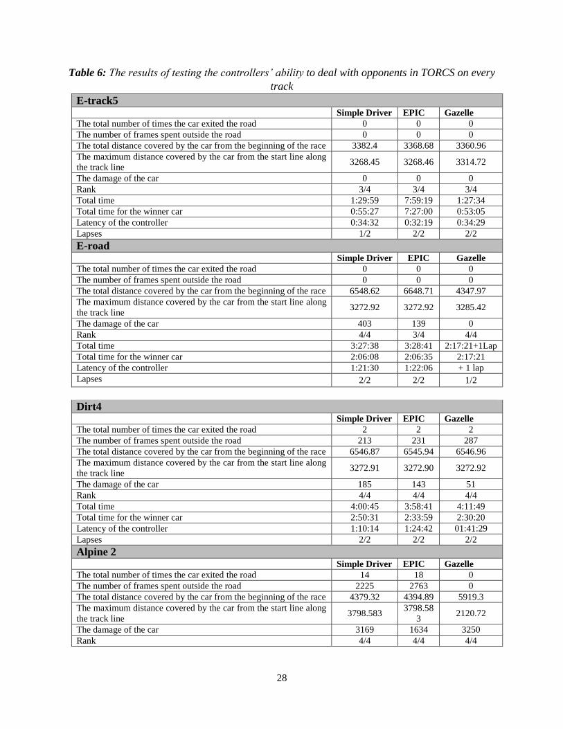
Table 6: The results of testing the controllers’ ability to deal with opponents in TORCS on every

track

E-track5 Simple Driver EPIC Gazelle



The total distance covered by the car from the beginning of the race 3382.4 3368.68 3360.96


the track line 3268.45 3268.46 3314.72


Rank 3/4 3/4 3/4

Total time 1:29:59 7:59:19 1:27:34

Total time for the winner car 0:55:27 7:27:00 0:53:05

Latency of the controller 0:34:32 0:32:19 0:34:29

Lapses 1/2 2/2 2/2

E-road Simple Driver EPIC Gazelle





the track line 3272.92 3272.92 3285.42


Rank 4/4 3/4 4/4

Total time 3:27:38 3:28:41 2:17:21+1Lap


Latency of the controller 1:21:30 1:22:06 + 1 lap

Lapses 2/2 2/2 1/2

Dirt4 Simple Driver EPIC Gazelle





the track line 3272.91 3272.90 3272.92


Rank 4/4 4/4 4/4

Total time 4:00:45 3:58:41 4:11:49


Latency of the controller 1:10:14 1:24:42 01:41:29

Lapses 2/2 2/2 2/2

Alpine 2






the track line 3798.583

3798.58

3 2120.72


Rank 4/4 4/4 4/4

29

Total time 3:06:17

+ 1 lap

3:06:17

+ 1 lap

3:03:11

+1 Lap


Latency of the controller + 1 lap + 1 lap + 1 lap

Lapses 1/2 1/2 1/2

Forza






the track line 2745.69 2745.78 5809.10


Rank 4/4 4/4 4/4

Total time 02:39:32

+2 laps

2:39:32

+ 2 laps

02:46:01

+1 Lap


Latency of the controller + 2 lap + 2 lap + 1 lap

Lapses 0/2 0/2 1/2

On E-track5, which is a fairly easy oval road, the three controllers presented similar results;

they didn’t get out of the track nor took any damage. Furthermore, all of them achieved the third

rank out of four racing cars. The Gazelle completed the race successfully in 1:27:34 average time

per second, and EPIC came in second with 6:31:45, while the Simple Driver couldn’t complete

the second lapse.

On E-Road, which is a wide road with a lot of curves, the Gazelle is the only controller

that failed to complete the race; this failure was due to reducing the speed to the safe speed when

the car was taking the curves. However, it succeeded in remaining inside the track during the race

without any damage while the two other controllers suffered medium damage caused either by

hitting the hard shoulders on the side of the road or by colliding with other opponents.

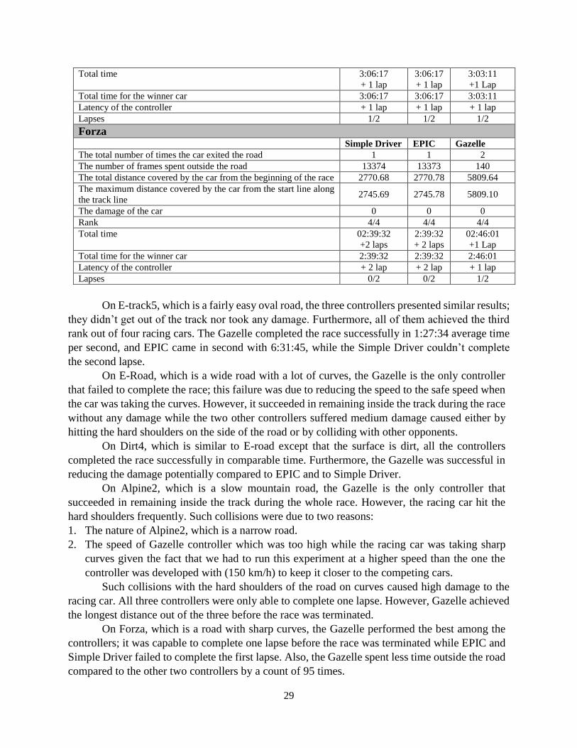
On Dirt4, which is similar to E-road except that the surface is dirt, all the controllers

completed the race successfully in comparable time. Furthermore, the Gazelle was successful in

reducing the damage potentially compared to EPIC and to Simple Driver.

On Alpine2, which is a slow mountain road, the Gazelle is the only controller that

succeeded in remaining inside the track during the whole race. However, the racing car hit the

hard shoulders frequently. Such collisions were due to two reasons:

1. The nature of Alpine2, which is a narrow road.

2. The speed of Gazelle controller which was too high while the racing car was taking sharp

curves given the fact that we had to run this experiment at a higher speed than the one the

controller was developed with (150 km/h) to keep it closer to the competing cars.

Such collisions with the hard shoulders of the road on curves caused high damage to the

racing car. All three controllers were only able to complete one lapse. However, Gazelle achieved

the longest distance out of the three before the race was terminated.

On Forza, which is a road with sharp curves, the Gazelle performed the best among the

controllers; it was capable to complete one lapse before the race was terminated while EPIC and

Simple Driver failed to complete the first lapse. Also, the Gazelle spent less time outside the road

compared to the other two controllers by a count of 95 times.

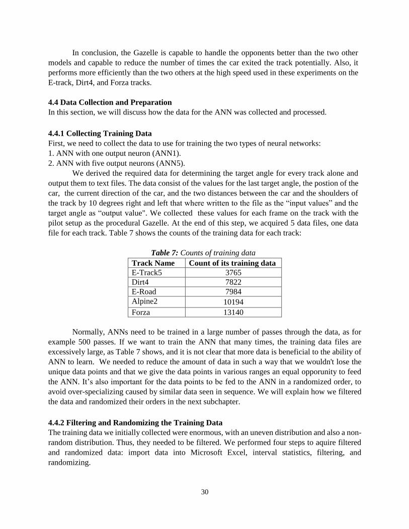
30

In conclusion, the Gazelle is capable to handle the opponents better than the two other

models and capable to reduce the number of times the car exited the track potentially. Also, it

performs more efficiently than the two others at the high speed used in these experiments on the

E-track, Dirt4, and Forza tracks.

4.4 Data Collection and Preparation

In this section, we will discuss how the data for the ANN was collected and processed.

4.4.1 Collecting Training Data

First, we need to collect the data to use for training the two types of neural networks:

1. ANN with one output neuron (ANN1).

2. ANN with five output neurons (ANN5).

We derived the required data for determining the target angle for every track alone and

output them to text files. The data consist of the values for the last target angle, the postion of the

car, the current direction of the car, and the two distances between the car and the shoulders of

the track by 10 degrees right and left that where written to the file as the “input values” and the

target angle as “output value". We collected these values for each frame on the track with the

pilot setup as the procedural Gazelle. At the end of this step, we acquired 5 data files, one data

file for each track. Table 7 shows the counts of the training data for each track:

Table 7: Counts of training data

Track Name Count of its training data

E-Track5 3765

Dirt4 7822

E-Road 7984

Alpine2 10194

Forza 13140

Normally, ANNs need to be trained in a large number of passes through the data, as for

example 500 passes. If we want to train the ANN that many times, the training data files are

excessively large, as Table 7 shows, and it is not clear that more data is beneficial to the ability of

ANN to learn. We needed to reduce the amount of data in such a way that we wouldn't lose the

unique data points and that we give the data points in various ranges an equal opporunity to feed

the ANN. It’s also important for the data points to be fed to the ANN in a randomized order, to

avoid over-specializing caused by similar data seen in sequence. We will explain how we filtered

the data and randomized their orders in the next subchapter.

4.4.2 Filtering and Randomizing the Training Data

The training data we initially collected were enormous, with an uneven distribution and also a non-

random distribution. Thus, they needed to be filtered. We performed four steps to aquire filtered

and randomized data: import data into Microsoft Excel, interval statistics, filtering, and

randomizing.

31

First step: Import into Microsoft Excel:

We imported all the data files into a Microsoft Excel workbook. Every data file was stored in a

separate worksheet containing a table holding the data.

Second step: Interval statistics:

In order to analyze the distribution of the collected data, we divided the Target Angle, which is the

output value, into several small intervals, as shown in Table 8. Each interval was assigned an

identifying number, also shown in Table 8.

Table 8: The numbers assigned to each interval of the target angle range

The interval The interval’s ID number

<= -0.5º 0

[-0.5º, -0.4º) 2

[-0.4º, -0.3º) 3

[-0.3º, -0.2º) 4

[-0.2, -0.1º) 5

[-0.1º, -0.01º) 6

[-0.01º, 0.01º) 7

[0.01º, 0.1º) 8

[0. 1º, 0.2º) 9

[0.2º, 0.3º) 10

[0.3º, 0.4º) 11

[0.4º, 0.5 º) 12

[0.5º, 0.6º) 13

>=0.6º 14

The length of every interval is 0.1º except between -0.01º and 0.01º, where we added a

smaller interval (length=0.02º), because the data are comprehensive around the zero when the

racing car is traveling on a straight line (the target angle is almost zero).

We assigned a number for the data belonging to the same interval by generating a statement

of conditions by a loop in Basic, to acquire the following formula: =IF(I1>-0.5,

IF(I1>-0.4,

IF(I1>-0.3,

...

IF(I1>0.5,

IF(I1>0.6,0,14)

,13)

...

,4)

,3)

,2)

Then we added a new column (let’s call it: Col K) to hold this formula for all the data and

to represent the corresponding number of the intervals from Table 8 based on the output value (the

target angle). We can see the count of data points (or size) in every interval for each track in the

following charts in Figure 12:

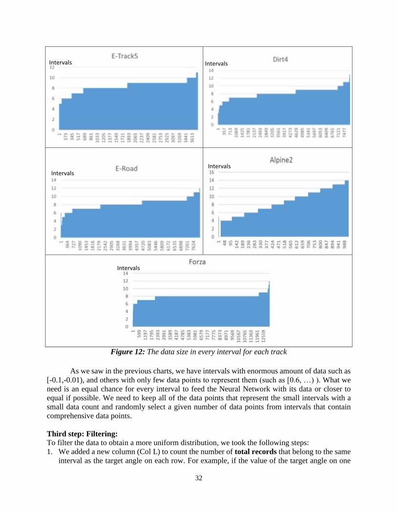
32

Figure 12: The data size in every interval for each track

As we saw in the previous charts, we have intervals with enormous amount of data such as

[-0.1,-0.01), and others with only few data points to represent them (such as [0.6, …) ). What we

need is an equal chance for every interval to feed the Neural Network with its data or closer to

equal if possible. We need to keep all of the data points that represent the small intervals with a

small data count and randomly select a given number of data points from intervals that contain

comprehensive data points.

Third step: Filtering: To filter the data to obtain a more uniform distribution, we took the following steps:

1. We added a new column (Col L) to count the number of total records that belong to the same

interval as the target angle on each row. For example, if the value of the target angle on one

Intervals Intervals

Intervals

Intervals

Intervals

33

row was 0.24 and the data file was for E-Road, then column L would show the count of the

data in the interval [0.2,0.3) for this track. To do this job, we applied the following formula to

(Col L): =COUNTIF(K:K,K1)

Where K1 is the value of the designated interval number, computed with the formula on page

31. This provides the count of the value of the cell K1 in the entire column K.

2. We assigned non-repeating random numbers to every data record belonging to the same

interval by generating random integer numbers between 0 and the total count of data in the

interval that the current target angle belongs to (Col L of the current row). We applied the

following formula to compute a new column (Col M): =RANDBETWEEN(0,L1)

This function generates a random integer number in the given range.

3. To get a reasonable amount of data in each interval, we filtered the data based on the random

numbers in Col M having values less than 50, which is the total count that we chose to keep in

each interval. This procedure will keep all the data that belong to small intervals of small counts

and also choose the right number of data from intervals that have comprehensive data. Table

9 shows some statistics of the count of data before and after filtering for each track.

Table 9: statistics of training data before/after filtering process

Track

Name

Data

before

filtering

Data

after

filtering

Percentage

of kept data

E-Track5 3765 398 11%

Dirt4 7822 745 10%

E-Road 7984 743 9%

Alpine2 10194 1060 10%

Forza 13140 604 5%

As a result, we reduced the size of data to the 11% of the original count in such a way that

we have a rational amount of data for every interval without neglecting the unique data that are

required to feed the ANN. The result of this procedure is shown in Figure 13.

34

Figure 13: the data size in every interval for each track. Before filtering (left), after filtering (right)

Intervals

Intervals

Intervals

Intervals

Intervals Intervals

Intervals

Intervals

Intervals

Intervals

Training Data Count Training Data Count

Training Data Count


Training Data Count



35

Forth step: Randomizing:

In this step we needed to sort the data randomly, such that the ANN is not over-trained by similar

data points being fed in sequence. For this part, we proceeded with the following operations:

1. Adding a new Column (Col J) to generate random fractional numbers between (0, 1) using: RAND()

2. Sorting the filtered table based on Col J.

After this step, the training data were filtered and randomized and they were ready to feed

the ANN. Figure 14 shows how the data distribution was like before and after the entire process

that we described in this section.

The charts before the filtering and randomizing process (on the right side in the charts)

show that the data are dense around the value 0 because the Target Direction Unit only changes

the target angle when there is an upcoming curve or the car is approaching the sides of the road.

Thus, the interval of 0 degrees contains redundant data which needed to be shredded. On the other

side, for large values of the target angle, the intervals contain less data, which means that we

needed all of them in such situations.

After the procedure (on the right side in the charts), the data became less redundant in the

comprehensive areas and the unique data from the sparse intervals were all kept.

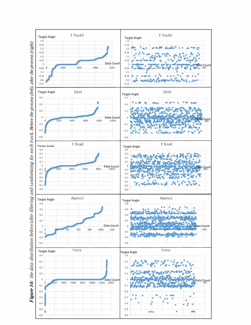
36

Target Angle

Target Angle

Target Angle

Target Angle

Target Angle

Data Count

Data Count

Data Count

Data Count

Data Count Data Count

Data Count

Data Count

Data Count

Data Count

Target Angle

Target Angle

Target Angle

Target Angle

Target Angle

Fig

ure

14:

the

data

dis

trib

uti

on b

efore

/aft

er f

ilte

ring a

nd r

andom

izin

g f

or

each

tra

ck.

Bef

ore

the

pro

cess

(le

ft),

aft

er t

he

pro

cess

(ri

ght)

37

4.5 Retrospective Testing of the ANN

After deriving the data from every track, the first evaluation step is retrospective, where the

training and testing tracks for the ANN are the same. Thus, we need to train the ANN on the data

file collected from a track, then we use it to drive the car on the same track. The procedure is

repeated for each of the five tracks. First, this will tell us if the ANN is capable of learning to

produce an appropriate target angle. Second, based on these results we can decide which data set

is more likely to work best with all the tracks. The reason we need to make such decision is that

during the competition the pilot will be faced with a track it has not seen before and we are trying

to prepare the best for this situation.

4.5.1 Testing Tracks

For the results in this section, we trained the ANN for each track using the data file collected on

the same track.

We set the maximum speed for all the situations we have tested to 150 km/h and the safe

speed to 100 km/h and we set the lapses to 2 lapses per race.

We trained the ANN with one neuron (NN1) and with five neurons (NN5) by repeating

the process of feeding the data and adapting the ANN to it by back-propagation in a large number

of iterations in an attempt to reduce the error value to the minimum. We experimented with

training the ANN over 100 iterations and over 500 iterations using one of two features: the last

weights values present in the ANN at the end of the training process or the best weights values

that were present in the ANN when the average error had the minimal value of the entire training

process. By combining the different alternatives for these settings, we trained the ANN by using

the data file for a track on the same track in 8 different models as shown in Tables 10 to 17.

1- ANN with 1 Neuron- 100 iterations- Last values Model:

Table 10: Results of applying ANN with 1 Neuron- 100 iterations- Last values Model

Etrack

5 Dirt4 E-Road Alpine2 Forza

The total number of times the car exited the road 37 65 65 3 1

The number of frames spent outside the road 5707 12395 12395 32 27791

The total distance covered by the car from the

beginning of the race 329.337 439 439 7572.02 2771.34

The maximum distance covered by the car from

the start line along the track line 304.337 414 414 3773.46 2746.34

The damage of the car 1115 2133 2133 0 0

Total time +1 lap +1 lap +1 lap 8:13:01 +1 lap

lapses 0/2 0/2 0/2 2/2 0/2

Table 10 shows the results obtained with one output neuron in 100 iterations, and using the

last values for the weights. On E-Track5, Dirt4 and E-Road, the racing car covered a short distance

and it got stuck a lot, which caused a high damage to the car. Meanwhile, the Alpine2 was the

best-performance track for this model because there was no damage and the car finished the race

successfully in an acceptable time. The total time was 8:13:01 minutes as compared to 5:32:39

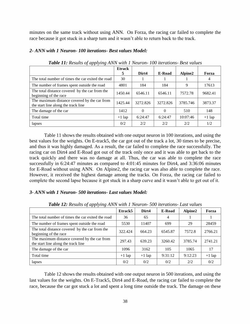
38

minutes on the same track without using ANN. On Forza, the racing car failed to complete the

race because it got stuck in a sharp turn and it wasn’t able to return back to the track.

2- ANN with 1 Neuron- 100 iterations- Best values Model:

Table 11: Results of applying ANN with 1 Neuron- 100 iterations- Best values

Etrack

5 Dirt4 E-Road Alpine2 Forza




beginning of the race 1450.44 6546.11 6546.11 7572.78 9682.41


the start line along the track line 1425.44 3272.826 3272.826 3785.746 3873.37


Total time +1 lap 6:24:47 6:24:47 10:07:46 +1 lap

lapses 0/2 2/2 2/2 2/2 1/2


best values for the weights. On E-track5, the car got out of the track a lot, 30 times to be precise,

and thus it was highly damaged. As a result, the car failed to complete the race successfully. The

racing car on Dirt4 and E-Road got out of the track only once and it was able to get back to the

track quickly and there was no damage at all. Thus, the car was able to complete the race

successfully in 6:24:47 minutes as compared to 4:01:45 minutes for Dirt4, and 3:36:06 minutes

for E-Road without using ANN. On Alpine2, the racing car was also able to complete the race.

However, it received the highest damage among the tracks. On Forza, the racing car failed to

complete the second lapse because it got stuck in a sharp curve and it wasn’t able to get out of it.

3- ANN with 1 Neuron- 500 iterations- Last values Model:

Table 12: Results of applying ANN with 1 Neuron- 500 iterations- Last values

Etrack5 Dirt4 E-Road Alpine2 Forza








Total time +1 lap +1 lap 9:31:12 9:12:23 +1 lap

lapses 0/2 0/2 0/2 2/2 0/2


last values for the weights. On E-Track5, Dirt4 and E-Road, the racing car failed to complete the

race, because the car got stuck a lot and spent a long time outside the track. The damage on these

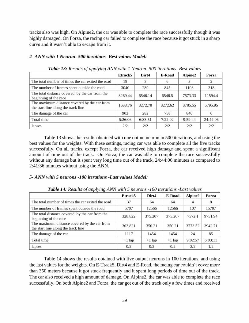
39

tracks also was high. On Alpine2, the car was able to complete the race successfully though it was

highly damaged. On Forza, the racing car failed to complete the race because it got stuck in a sharp

curve and it wasn’t able to escape from it.

4- ANN with 1 Neuron- 500 iterations- Best values Model:

Table 13: Results of applying ANN with 1 Neuron- 500 iterations- Best values









Total time 5:26:06 6:33:51 7:22:02 9:59:44 24:44:06

lapses 2/2 2/2 2/2 2/2 2/2


best values for the weights. With these settings, racing car was able to complete all the five tracks

successfully. On all tracks, except Forza, the car received high damage and spent a significant

amount of time out of the track. On Forza, the car was able to complete the race successfully

without any damage but it spent very long time out of the track, 24:44:06 minutes as compared to

2:41:36 minutes without using the ANN.

5- ANN with 5 neurons -100 iterations -Last values Model:

Table 14: Results of applying ANN with 5 neurons -100 iterations -Last values









Total time +1 lap +1 lap +1 lap 9:02:57 6:03:11

lapses 0/2 0/2 0/2 2/2 1/2

Table 14 shows the results obtained with five output neurons in 100 iterations, and using

the last values for the weights. On E-Track5, Dirt4 and E-Road, the racing car couldn’t cover more

than 350 meters because it got stuck frequently and it spent long periods of time out of the track.

The car also received a high amount of damage. On Alpine2, the car was able to complete the race

successfully. On both Alpine2 and Forza, the car got out of the track only a few times and received

40

less damage than on the three other tracks. On Forza, the racing car got stuck for a long time in a

sharp curve and thus it failed to complete the race to the end.

6- ANN with 5 neurons -100 iterations - Best values Model:

Table 15: Results of applying ANN with 5 neurons -100 iterations - Best values









Total time +1 lap 6:22:51 6:22:51 8:12:57 11:44:21

lapses 0/2 2/2 2/2 2/2 2/2


the best values for the weights. On E-Track5, the racing car was able to cover only two thirds of

the first lapse because it got stuck many times for long periods of time. On this track, the car

received a medium amount of damage. On the rest of the tracks, the car was able to complete the

race within acceptable time and the damage was low for all of them. On Forza, the car performed

the best among other models and it was able to complete the race successfully.

7- ANN with 5 neurons -500 iterations -Last values Model:

Table 16: Results of applying ANN with 5 neurons -500 iterations -Last values









Total time +1 lap +1 laps 8:57:33 9:25:59 +1 lap

lapses 0/2 0/2 2/2 2/2 0/2


the last values for the weights. The racing car wasn’t able to complete the first lapse since it got

stuck a lot except on E-road and Alpine2. However, on Alpine2, the car received potentially high

damage. On E-Road, the racing car received low damage and spent a minor period of time out of

the track.

41

8- ANN with 5 neurons -500 iterations-Best values Model:

Table 17: Results of applying ANN with 5 neurons -500 iterations-Best values





beginning of the race 3268.19

6546.0

1 6548.42 7572.28 11595.7

The maximum distance covered by the car from the

start line along the track line 1621.46

3272.8

5 3271.6 3786.7 5795.5


Total time 4:17:39 6:23:22 5:49:23 10:41:56 12:22:19

lapses 2/2 2/2 2/2 2/2 2/2


the best values for the weights. The racing car was able to complete the race on all the five tracks.

On E-track, the car got stuck frequently and it received high damage. On Dirt4, the car got stuck

only once and it received a low amount of damage. On E-Road, the car also got stuck only once

but it didn’t receive any damage. On Alpine2, the car performed the best among the tracks using

the current model and it neither got stuck nor received any damage.

Choosing the best-performance model:

As we saw in the previous tables, on E-Track on all models, the racing car easily got stuck and it

received high damage because the data file collected on this track reflects the fact that this track

features only wide curves that are not very challenging for the driver. Thus, when the car gets

stuck, it can’t adjust the target angle properly to maintain traveling inside the track, having seen

only smaller angles.

On Dirt4 and E-Road, the racing car behaved similarly and such similar behavior is due to

the fact that both Dirt4 and E-Road have the same properties except the material is different. Dirt4

is muddy and E-Road is made of asphalt. On both tracks, the racing car spent a long time to get

back to the track every time it got stuck and this happened with every variation of the ANN

parameters we have tried, which wastes more time. It completed the race only when the ANN was

using the best values.

On Forza, the racing car couldn’t complete the race in most models. Such a failure is due

to the track shape which contains only sharp turns. Thus, when the car gets stuck in a sharp curve,

it can't return back properly to the track because the collected data were limited to deal only with

wider angles than the sharp curves involve.

On Alpine2, in general, the racing car did its best among all the tracks for all the settings

of the ANN and it completed the race successfully in every setting. This success is due to the shape

of the track, which contains many various types of curves. As a result, the ANN is trained better

with its data file. We can choose Alpine2 as the best track so far.

After all the experiments, we can nominate Alpine 2 as the ideal track to use with our ANN.

We can also see that using the data collected from Alpine2 with the model of 5 output neurons

seems to perform better than the model of 1 output neuron. Additionally, using the best weights

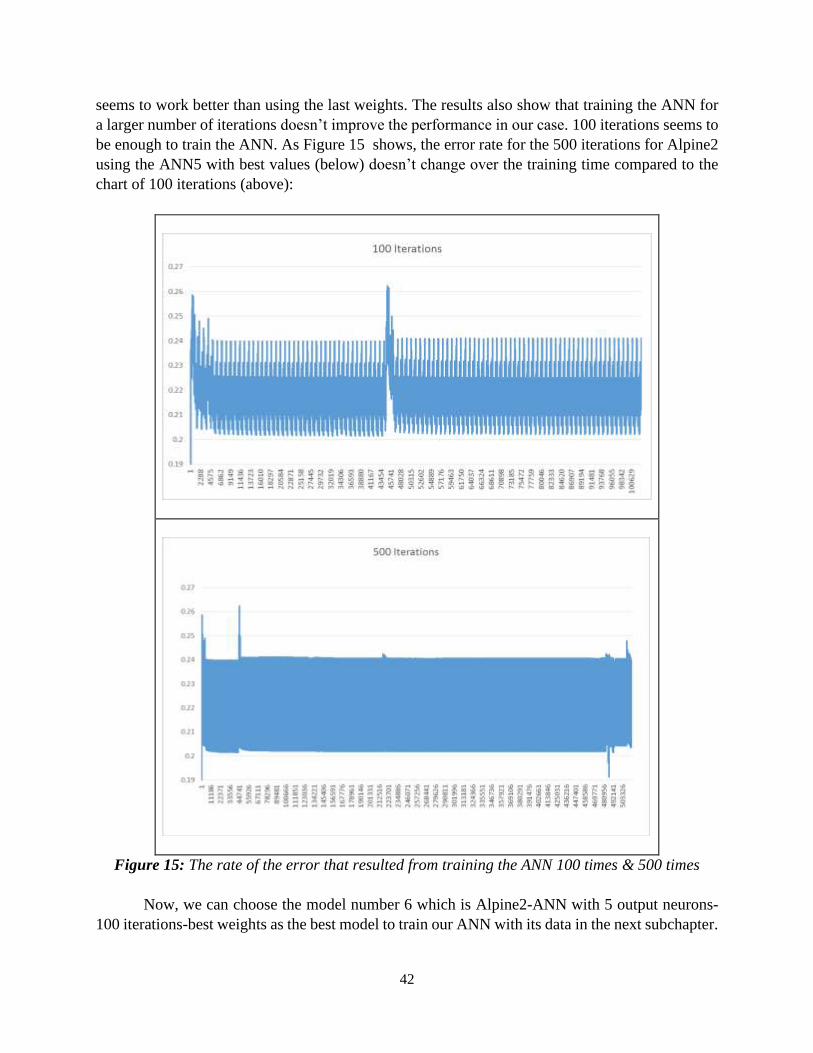
42

seems to work better than using the last weights. The results also show that training the ANN for

a larger number of iterations doesn’t improve the performance in our case. 100 iterations seems to

be enough to train the ANN. As Figure 15 shows, the error rate for the 500 iterations for Alpine2

using the ANN5 with best values (below) doesn’t change over the training time compared to the

chart of 100 iterations (above):

Figure 15: The rate of the error that resulted from training the ANN 100 times & 500 times

Now, we can choose the model number 6 which is Alpine2-ANN with 5 output neurons-

100 iterations-best weights as the best model to train our ANN with its data in the next subchapter.

43

4.6 Testing the ANN with the New Tracks

For this part of experiments, we tried to see how well the pilot with the ANN can perform when it

is trained from the data obtained from one track and then tested on a new track. We used the

approach that had the best result in the experiments presented in the previous section, which is

Alpine 2 with ANN5 and 100 training steps and the best weights after training, on all the tracks.

We trained the ANN with the data file for this track first, then we used it on every track with the

given settings. Table 18 shows the experimental results of applying the data file of Alpine2 on

every track.

Table 18: Results of applying data of Alpine2 for training ANN on all of the five tracks

With ANN


The total number of times the car exited the

road 0 12 4 0 2







Total time 3:36:25 10:23:57 8:30:35 8:12:57 +1lap

lapses 2/2 2/2 2/2 2/2 0/2

Without ANN


The total number of times the car exited the

road 0 0 0 1 4





the start line along the track line 1621.04 3260.19 3,272.82 3773.55 5784.09


Total time 1:27:10 1:27:10 1:27:10 5:32:39 2:41:36

lapses 2/2 2/2 2/2 2/2 2/2

On E-track5, the ANN with weights obtained from training the ANN with the data of

Alpine2 was efficient and the racing car was able to complete the race successfully without any

damage and within a tolerable time. However, the car spent nearly twice the time that the car spent

to complete the race on the same track without using the ANN.

On E-Road and on Dirt4, the racing car got out of the track frequently and it spent a long

time to return back to the track. As a consequence, it took a longer time to complete the race when

it using the ANN than the spent time without using the ANN. However, it completed the race

successfully without any damage on E-road and medium damage on Dirt4.

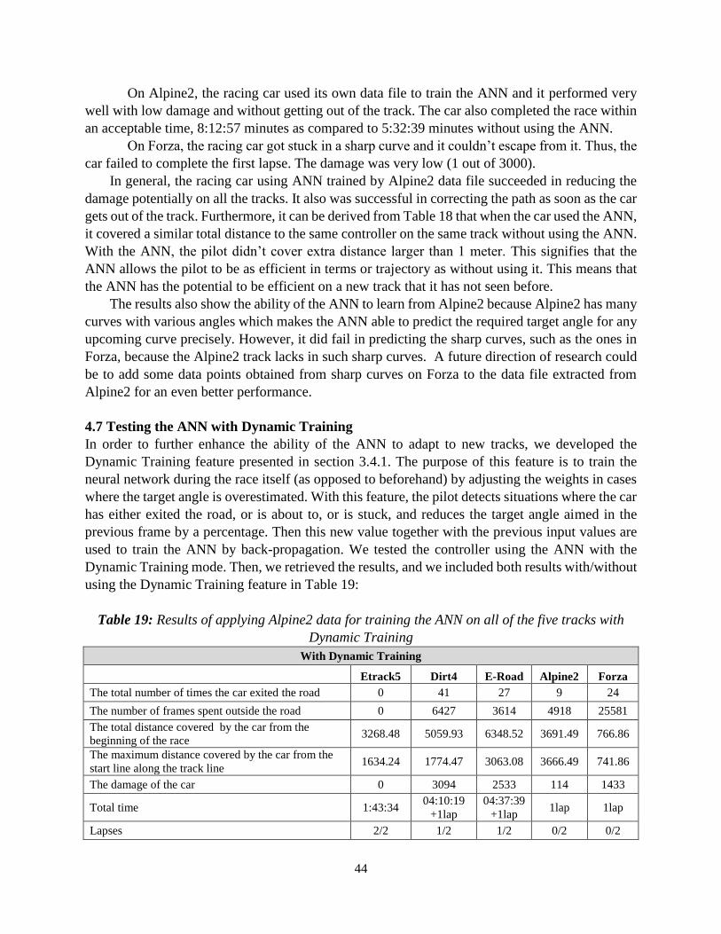
44

On Alpine2, the racing car used its own data file to train the ANN and it performed very

well with low damage and without getting out of the track. The car also completed the race within

an acceptable time, 8:12:57 minutes as compared to 5:32:39 minutes without using the ANN.

On Forza, the racing car got stuck in a sharp curve and it couldn’t escape from it. Thus, the

car failed to complete the first lapse. The damage was very low (1 out of 3000).

In general, the racing car using ANN trained by Alpine2 data file succeeded in reducing the

damage potentially on all the tracks. It also was successful in correcting the path as soon as the car

gets out of the track. Furthermore, it can be derived from Table 18 that when the car used the ANN,

it covered a similar total distance to the same controller on the same track without using the ANN.

With the ANN, the pilot didn’t cover extra distance larger than 1 meter. This signifies that the

ANN allows the pilot to be as efficient in terms or trajectory as without using it. This means that

the ANN has the potential to be efficient on a new track that it has not seen before.

The results also show the ability of the ANN to learn from Alpine2 because Alpine2 has many

curves with various angles which makes the ANN able to predict the required target angle for any

upcoming curve precisely. However, it did fail in predicting the sharp curves, such as the ones in

Forza, because the Alpine2 track lacks in such sharp curves. A future direction of research could

be to add some data points obtained from sharp curves on Forza to the data file extracted from

Alpine2 for an even better performance.

4.7 Testing the ANN with Dynamic Training

In order to further enhance the ability of the ANN to adapt to new tracks, we developed the

Dynamic Training feature presented in section 3.4.1. The purpose of this feature is to train the

neural network during the race itself (as opposed to beforehand) by adjusting the weights in cases

where the target angle is overestimated. With this feature, the pilot detects situations where the car

has either exited the road, or is about to, or is stuck, and reduces the target angle aimed in the

previous frame by a percentage. Then this new value together with the previous input values are

used to train the ANN by back-propagation. We tested the controller using the ANN with the

Dynamic Training mode. Then, we retrieved the results, and we included both results with/without

using the Dynamic Training feature in Table 19:

Table 19: Results of applying Alpine2 data for training the ANN on all of the five tracks with

Dynamic Training

With Dynamic Training







start line along the track line 1634.24 1774.47 3063.08 3666.49 741.86


Total time 1:43:34 04:10:19

+1lap

04:37:39

+1lap 1lap 1lap

Lapses 2/2 1/2 1/2 0/2 0/2

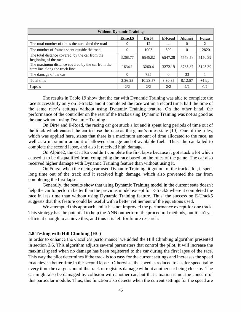
45

Without Dynamic Training







start line along the track line 1634.1 3260.4 3272.19 3785.37 5125.39


Total time 3:36:25 10:23:57 8:30:35 8:12:57 +1lap

Lapses 2/2 2/2 2/2 2/2 0/2

The results in Table 19 show that the car with Dynamic Training was able to complete the

race successfully only on E-track5 and it completed the race within a record time, half the time of

the same race’s settings without using Dynamic Training feature. On the other hand, the

performance of the controller on the rest of the tracks using Dynamic Training was not as good as

the one without using Dynamic Training.

On Dirt4 and E-Road, the racing car got stuck a lot and it spent long periods of time out of

the track which caused the car to lose the race as the game’s rules state [10]. One of the rules,

which was applied here, states that there is a maximum amount of time allocated to the race, as

well as a maximum amount of allowed damage and of available fuel. Thus, the car failed to

complete the second lapse, and also it received high damage.

On Alpine2, the car also couldn’t complete the first lapse because it got stuck a lot which

caused it to be disqualified from completing the race based on the rules of the game. The car also

received higher damage with Dynamic Training feature than without using it.

On Forza, when the racing car used Dynamic Training, it got out of the track a lot, it spent

long time out of the track and it received high damage, which also prevented the car from

completing the first lapse.

Generally, the results show that using Dynamic Training model in the current state doesn't

help the car to perform better than the previous model except for E-track5 where it completed the

race in less time than without using Dynamic Training feature. Thus, the success on E-Track5

suggests that this feature could be useful with a better refinement of the equations used.

We attempted this approach and it has not improved the performance except for one track.

This strategy has the potential to help the ANN outperform the procedural methods, but it isn't yet

efficient enough to achieve this, and thus it is left for future research.

4.8 Testing with Hill Climbing (HC)

In order to enhance the Gazelle’s performance, we added the Hill Climbing algorithm presented

in section 3.6. This algorithm adjusts several parameters that control the pilot. It will increase the

maximal speed when no damage has been registered to the car during the first lapse of the race.

This way the pilot determines if the track is too easy for the current settings and increases the speed

to achieve a better time in the second lapse. Otherwise, the speed is reduced to a safer speed value

every time the car gets out of the track or registers damage without another car being close by. The

car might also be damaged by collision with another car, but that situation is not the concern of

this particular module. Thus, this function also detects when the current settings for the speed are

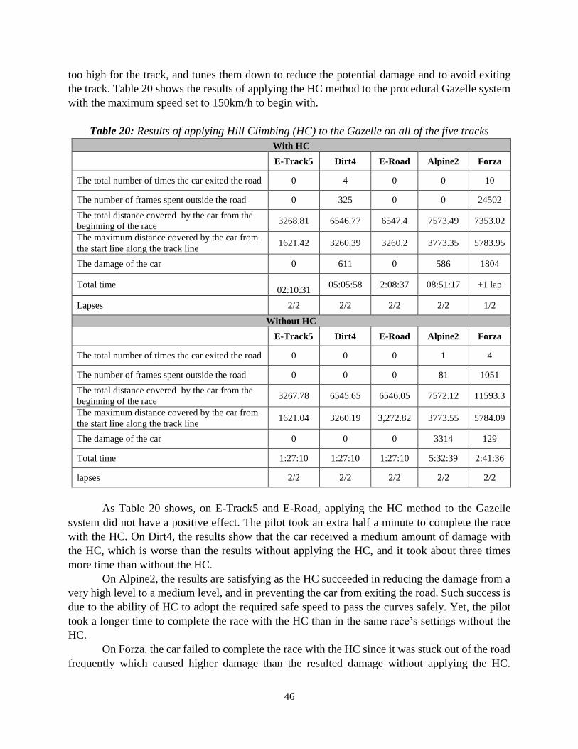
46

too high for the track, and tunes them down to reduce the potential damage and to avoid exiting

the track. Table 20 shows the results of applying the HC method to the procedural Gazelle system

with the maximum speed set to 150km/h to begin with.

Table 20: Results of applying Hill Climbing (HC) to the Gazelle on all of the five tracks

With HC

E-Track5 Dirt4 E-Road Alpine2 Forza








Total time

02:10:31 05:05:58 2:08:37 08:51:17 +1 lap

Lapses 2/2 2/2 2/2 2/2 1/2

Without HC







the start line along the track line 1621.04 3260.19 3,272.82 3773.55 5784.09


Total time 1:27:10 1:27:10 1:27:10 5:32:39 2:41:36

lapses 2/2 2/2 2/2 2/2 2/2

As Table 20 shows, on E-Track5 and E-Road, applying the HC method to the Gazelle

system did not have a positive effect. The pilot took an extra half a minute to complete the race

with the HC. On Dirt4, the results show that the car received a medium amount of damage with

the HC, which is worse than the results without applying the HC, and it took about three times

more time than without the HC.

On Alpine2, the results are satisfying as the HC succeeded in reducing the damage from a

very high level to a medium level, and in preventing the car from exiting the road. Such success is

due to the ability of HC to adopt the required safe speed to pass the curves safely. Yet, the pilot

took a longer time to complete the race with the HC than in the same race’s settings without the

HC.

On Forza, the car failed to complete the race with the HC since it was stuck out of the road

frequently which caused higher damage than the resulted damage without applying the HC.

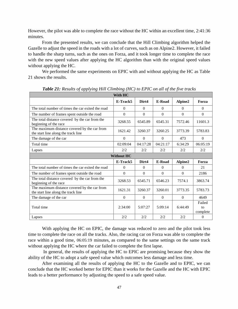
47

However, the pilot was able to complete the race without the HC within an excellent time, 2:41:36

minutes.

From the presented results, we can conclude that the Hill Climbing algorithm helped the

Gazelle to adjust the speed in the roads with a lot of curves, such as on Alpine2. However, it failed

to handle the sharp turns, such as the ones on Forza, and it took longer time to complete the race

with the new speed values after applying the HC algorithm than with the original speed values

without applying the HC.

We performed the same experiments on EPIC with and without applying the HC as Table

21 shows the results.

Table 21: Results of applying Hill Climbing (HC) to EPIC on all of the five tracks

With HC









Total time 02:09:04 04:17:28 04:21:17 6:34:29 06:05:19

Lapses 2/2 2/2 2/2 2/2 2/2

Without HC









Total time 2:34:00 5:07:27 5:09:14 6:44:49

Failed

to

complete

Lapses 2/2 2/2 2/2 2/2 0

With applying the HC on EPIC, the damage was reduced to zero and the pilot took less

time to complete the race on all the tracks. Also, the racing car on Forza was able to complete the

race within a good time, 06:05:19 minutes, as compared to the same settings on the same track

without applying the HC where the car failed to complete the first lapse.

In general, the results of applying the HC to EPIC are promising because they show the

ability of the HC to adopt a safe speed value which outcomes less damage and less time.

After examining all the results of applying the HC to the Gazelle and to EPIC, we can

conclude that the HC worked better for EPIC than it works for the Gazelle and the HC with EPIC

leads to a better performance by adjusting the speed to a safe speed value.

48

5. Conclusions In the thesis, we hoped to accomplish a well-developed and efficient algorithm for Gazelle. Such

an algorithm can be improved by the learning methods using neural networks and Hill Climbing.

We aimed to lead the racing car to achieve an efficient path and an efficient speed and to minimize

the damage caused either by opponents or by getting out of the track. For this, we used procedural

and learning methods to enable the controller to make a good decision in every frame of the race.

As part of this project, we participated in an international competition (GECCO-13). The

procedural Gazelle code was submitted to a TORCS competition where it was accepted and

qualified to be a part of the final race. AUTOPIA was the winner of GECCO-2013 SCR whereas

our car achieved the eighth rank as the champion’s organizers announced [23]. Table 22 shows a

summary of the championship's results.

Table 22: Results summary for GECCO-13 [23]

Competitor Alsoujlak Arraias Sancassa Total

AUTOPIA 12 13 13 38

MrRacer 9 5.5 6 20.5

ICER-IDDFS 6 5 8 19

GRNDriver 5 5.5 4 14.5

SnakeOil 3 7 3.5 13.5

Presto AI 3 1 5 9

EVOR 3 4 1 8

GAZELLE 1.5 3 2 6.5

Our controller was submitted before developing the learning methods, thus the damage was

high, which affected on the performance negatively, and the pilot achieved lower scores for the

tracks: Alsoujalk, Arraias, and Sancassa.

This participation inspired us to continue developing our controller to be a part of the next

year’s competitions for simulated racing car. For this, we refined the procedural methods, added

learning components, and added an opponent modifier module. Our ongoing efforts to develop the

Gazelle controller aimed to predict an appropriate path and speed for the racing car in each frame

of the race based on the available information about the car's state and based on the knowledge

that the car has built using the learning methods. For this, we used both procedural methods and a

neural network. We hoped that using neural networks could lead the controller to derive more

accurate equations based on previous data acquired during the training process. We also expected

that the more the networks are trained, the more precisely they would predict the driving

information. We also used a Hill Climbing method to refine the learning process.

In this work, we implemented several procedural methods to improve the performance of

the Gazelle. We developed the Target Direction Unit to predict the target angle more precisely.

We also developed the Target Speed Unit to determine an appropriate speed based on the target

angle, with the goal to achieve the maximum allowed speed when the path is almost straight, and

a safe speed when the pilot is taking curves. We also added the Opponent Adjuster for handling

the opponents if they violate chosen tolerance values of closeness as determined by the opponent

49

sensors in each direction, by modifying the speed value and the steering angle to avoid the

collision.

In addition to the procedural units, we added the Trouble Spot Register which avoids the

accidents caused by errors in predicting the right steering angle that causes the car to get out of the

track. We also used several learning methods to optimize the performance of the procedural

Gazelle by enabling the controller to learn during the race using learning algorithms. We employed

two main learning algorithms: Neural Networks and Hill Climbing. We substituted the procedural

Target Direction Unit with an ANN system. The ANN calculates the appropriate target angle after

training the ANN with the data file extracted while using the procedural units. We also enhanced

the ANN by the Dynamic Training feature for adjusting the weights of the ANN during the race

in cases where the target angle is overestimated. We also used the Hill Climbing algorithm to

adjust the speed of the car to reach the maximum safe value during the race.

The results show that using the ANN helped to avoid the damage on some tracks and helped

to minimize the damage on others. The results also show that the ANN was able to learn from

Alpine2 the best because it has many curves with various angles. This allows the ANN to predict

the required target angle for any upcoming curve precisely. However, the ANN needs more data

acquired on sharp curves to enable the ANN to predict the accurate required target angle for sharp

curves, such as the ones on Forza, and to return back to the track with a sharp steering angle when

the racing car gets out of the track. The results also show that using the Dynamic Training model

to enhance the performance of the ANN has not improved the performance except for E-track5

and refining the used equations more is needed for a better performance. The results also show

that the Hill Climbing algorithm (HC) improved the car’s performance in situations where the road

has a lot of curves, such as the Alpine2 track. The HC helped to reduce the damage by adopting

safe speed values in the curves. However, the HC made the pilot take a longer time to finish the

race with a lower amount of damage than the required time without applying the HC.

After all these experiments, we can conclude that the Gazelle is an improvement over EPIC

because the Gazelle was able to handle the opponents efficiently and it succeeded in avoiding the

damage caused either by colliding with other opponents or by hitting the hard shoulders on the

side of the road. Also, we can conclude that using the ANN helped the Gazelle to behave more

efficiently on any new tracks of any type or any shape. Even though, the Gazelle took a longer

time to complete the race with the ANN as compared to the procedural methods with the same

settings without using the ANN, we can adopt a higher value for the maximum speed for the next

competition. Additionally, the HC algorithm was useful in situations where the road has a lot of

curves, such as Alpine2, since it helped to adopt safe speed values to pass these curves without

causing any damage. Yet, the HC took extra time as a result of adopting variant speed values.

Working with such a project helped us to improve our skills with programming using C++. It

also introduced us to game programing and new learning methods such as neural networks and

Hill Climbing. This thesis fulfilled our passion to make the Gazelle system a self-training

controller and we hope to achieve a higher ranking in the next international championship. We

will continue developing on this project to submit it to the same competition this year.

50

6. References

[1] D. Aryal, W. Yao-wu, (2003), “Neural Network Forecasting of the Production Level of Chinese

Construction Industry”, Journal of Competitive International management, vol. 6, No. 2.

[2] A. Blum, R.L. Rivest, (1989), “Training a 3-node neural network is NP-complete, in Touretzky,

D.S.” (ed.), Advances in Neural Information Processing Systems, San Mateo, CA: Morgan

Kaufmann, 494-501.

[3] N. Chaudhary and S. Sharma (2013). Race Car Strategy Optimization under Simulation. April

2013, 1-7.

[4] S.E. Fahlman and C. Lebiere (1990). “The Cascade Correlation Learning Architecture,” NIPS2,

524-532.

[5] C. Guse and D. Vrajitoru (2010). “The EPIC Adaptive Car Pilot.” In Proceedings of the

Midwest Artificial Intelligence and Cognitive Science Conference, April 17-18, South Bend, IN,

30-35.

[6] K. Hornik, (1993). “Some new results on neural network approximation,” Neural Networks, 6,

1069-1072.

[7] T. S. Kim, J. C. Na, et al. (2012). “Optimization of an Autonomous Car Controller using a Self-

Adaptive Evolutionary Strategy.” Published in International Journal of Advanced Robotic

Systems, vol. 9, 73, 1-15.

[8] M. Kole, A. Etaner-Uyar, et al. (2012). “Heuristics for car setup optimisation in TORCS.” In

proceeding of IEEE Symposium on Computational Intelligence and Games, 2012, Edinburgh, UK,

1-8.

[9] R. Lopez, (2012). OpenNN: Open Neural Networks Library Software Manual.

[10] D. Loiacono, L. Cardamone, et al. (2013). Simulated Racing car Championship Competition

Software Manual, April 2013.

[11] P. McCullagh, J.A. Nelder, (1989). Generalized Linear Models, 2nd edition. London, UK:

Chapman and Hall/CRC Press

[12] J. Mun˜oz, G. Gutierrez, et al. (2010). “A Human-like TORCS Controller for the Simulated

Racing car Championship.” Published in IEEE Symposium on Computational Intelligence and

Games (CIG), 473 - 480.

[13] E. Onieva, D. A. Pelta, et al. (2009). “A Modular Parametric Architecture for the TORCS

Racing Engine.” In proceeding of IEEE Symposium on Computational Intelligence and Games,

2009, Madrid, Spain, 256-262.

[14] E. Onieva, D. A. Pelta, et al. (2012). “An Evolutionary Tuned Driving System for Virtual

Racing car Games: The AUTOPIA Driver.” Published in International Journal of Intelligent

Systems 27, 3, Oct 2012, Madrid, Spain, 217-241

[15] J. Quadflieg, M. Preuss, et al. (2010). “Learning the Track and Planning Ahead in a Racing

car Controller.” Published in IEEE Conference on Computational Intelligence and Games

(CIG’10), 395-402

[16] G. Raidl, (2009). Proceedings of the Genetic and Evolutionary Computation Conference

(GECCO). Montreal, Canada: ACM SIGEVO.

[17] S. Russell, P. Norvig, (2009). Artificial Intelligence: A Modern Approach, 3rd edition. New

Jersey: Prentice Hall, 122-125.

51

[18] K. Swingler, (1996). Applying Neural Networks: A Practical Guide, London: Academic Press.

[19] T. Weise, (2009). Global Optimization Algorithms: Theory and Application, 2nd Edition.

Thomas Weise.

[20] L. A. Zadeh, (1965). “Fuzzy Sets,” Information and Control, vol. 8, 338–353.

[21] The Center for Automotive Research at Stanford

(http://me.stanford.edu/groups/design/automotive/)

[22] Neural Network (http://www.doc.ic.ac.uk/~nd/surprise_96/journal/vol4/cs11/report.html )

[23] 2013 Simulated Racing Car (GECCO-2013).

(http://www.slideshare.net/dloiacono/gecco13scr)

[24] Neural Networks history,

(http://www-cs-faculty.stanford.edu/~eroberts/courses/soco/projects/neural-networks/)

[25] Usenet newsgroup (ftp://ftp.sas.com/pub/neural/FAQ3.html)

[26] D. Miller, (2011). Make a Neural Net Simulator in C++,

(http://www.millermattson.com/dave/?p=54)

http://me.stanford.edu/groups/design/automotive/

http://www.doc.ic.ac.uk/~nd/surprise_96/journal/vol4/cs11/report.html#What is a Neural Network

ftp://ftp.sas.com/pub/neural/FAQ3.html

http://www.millermattson.com/dave/?p=54

“the gazelle adaptive racing car pilot abstract in this thesis, we developed a car driving system...

Documents