the gaseous environment of radio galaxies: a … · 4.2 warm absorber modelling . . . . . . . . . ....
TRANSCRIPT

Alma Mater Studiorum
Universita degli Studi di Bologna
Facolta di Scienze Matematiche, Fisiche e Naturali
Dipartimento di Astronomia
DOTTORATO DI RICERCA IN ASTRONOMIA
Ciclo XXIII
THE GASEOUS ENVIRONMENT OF RADIO GALAXIES:
A NEW PERSPECTIVE FROM
HIGH–RESOLUTION X–RAY SPECTROSCOPY
di
ELEONORA TORRESI
Coordinatore:
Chiar.mo Prof.
LAURO MOSCARDINI
Relatore:
Chiar.mo Prof.
GIORGIO G.C. PALUMBO
Co–Relatrice:
Dr.ssa PAOLA GRANDI
Settore Scientifico Disciplinare: Area 02 - Scienze Fisiche
FIS/05 Astronomia e Astrofisica
Esame finale anno 2011


This thesis has been carried out at INAF/IASF-Bologna
as part of the institute research activities
Contents
Contents 1
Abstract 11
1 Introduction 15
1.1 Active Galactic Nuclei . . . . . . . . . . . . . . . . . . . . . . . . 15
1.1.1 AGN classification and the Unified Model . . . . . . . . . 21
1.1.2 Radio galaxies . . . . . . . . . . . . . . . . . . . . . . . . 24
1.2 Accretion and jet link . . . . . . . . . . . . . . . . . . . . . . . . 30
1.2.1 Accretion . . . . . . . . . . . . . . . . . . . . . . . . . . . 30
1.2.2 Jets . . . . . . . . . . . . . . . . . . . . . . . . . . . . . . 34
1.2.3 Physical processes in jets . . . . . . . . . . . . . . . . . . 35
1.2.4 Jet orientation . . . . . . . . . . . . . . . . . . . . . . . . 36
1.3 Radio Loud AGNs in the Fermi era . . . . . . . . . . . . . . . . 38
1.3.1 Misaligned AGNs as a new class of GeV emitters . . . . . 39
1.3.2 The jet structure of NGC 6251 . . . . . . . . . . . . . . . 45
2 High resolution X–ray spectroscopy 49
2.1 Atomic processes and line diagnostics . . . . . . . . . . . . . . . 51
2.1.1 Radiation–driven processes . . . . . . . . . . . . . . . . . 52
2.1.2 Properties of photoionized plasmas . . . . . . . . . . . . . 56
2.1.3 Plasma diagnostics . . . . . . . . . . . . . . . . . . . . . . 59
2.1.4 Absorption . . . . . . . . . . . . . . . . . . . . . . . . . . 66
3 Warm photoionized gas in emission 69
3.1 Evidence of photoionized gas in the soft X–ray spectrum of 3C 33 71
3.1.1 Introduction . . . . . . . . . . . . . . . . . . . . . . . . . 72
3.1.2 Observations and data reduction . . . . . . . . . . . . . . 73
1
3.1.3 Spectral analysis . . . . . . . . . . . . . . . . . . . . . . . 75
3.1.4 Results . . . . . . . . . . . . . . . . . . . . . . . . . . . . 81
3.1.5 The origin of the soft X–ray emission . . . . . . . . . . . . 83
3.1.6 Summary . . . . . . . . . . . . . . . . . . . . . . . . . . . 85
4 Warm photoionized gas in absorption 87
4.1 Introduction . . . . . . . . . . . . . . . . . . . . . . . . . . . . . 87
4.2 Warm absorber modelling . . . . . . . . . . . . . . . . . . . . . . 88
4.3 First evidence of a warm absorber in the BLRG 3C 382 . . . . . 89
4.3.1 Introduction . . . . . . . . . . . . . . . . . . . . . . . . . 89
4.3.2 Observation and data reduction . . . . . . . . . . . . . . . 90
4.3.3 RGS data analysis . . . . . . . . . . . . . . . . . . . . . . 90
4.3.4 Localization of the warm absorber . . . . . . . . . . . . . 95
4.3.5 Summary . . . . . . . . . . . . . . . . . . . . . . . . . . . 96
4.4 Warm Absorbers in other BLRGs . . . . . . . . . . . . . . . . . 97
4.4.1 Introduction . . . . . . . . . . . . . . . . . . . . . . . . . 97
4.4.2 Data analysis . . . . . . . . . . . . . . . . . . . . . . . . . 98
4.4.3 3C 390.3 results . . . . . . . . . . . . . . . . . . . . . . . 99
4.4.4 3C 120 results . . . . . . . . . . . . . . . . . . . . . . . . 103
5 A small sample of Broad Line Radio Galaxies 107
5.1 Warm Absorber Physical Properties . . . . . . . . . . . . . . . . 107
5.2 Warm Absorber Energetics in BLRGs . . . . . . . . . . . . . . . 109
5.3 Comparison between radio–loud and radio–quiet WAs . . . . . . 112
6 Discussion and Conclusions 117
6.1 Future perspectives . . . . . . . . . . . . . . . . . . . . . . . . . 119
A The XMM–Newton observatory 123
A.1 Basic characteristics . . . . . . . . . . . . . . . . . . . . . . . . . 123
A.2 The X–ray telescopes . . . . . . . . . . . . . . . . . . . . . . . . 127
A.3 The EPIC cameras . . . . . . . . . . . . . . . . . . . . . . . . . 130
A.4 The RGS . . . . . . . . . . . . . . . . . . . . . . . . . . . . . . . 132
A.5 The OM . . . . . . . . . . . . . . . . . . . . . . . . . . . . . . . 132
B The Chandra X–ray observatory 135
2

C The IXO satellite 141
Acknowledgements 145
I Bibliography 147
Publications 157
3

4

List of Figures
List of Figures 5
1.1 Typical SED of an AGN from radio to X–rays. . . . . . . . . . . 16
1.2 Schematic representation of the 2–phase model. . . . . . . . . . . 18
1.3 PL continuum produced by multiple Compton scatterings. . . . . 18
1.4 Typical Seyfert 1 X–ray spectrum in the 0.1–200 keV band. . . . 20
1.5 Symmetric profiles on a non–relativistic disk and line distortion . 20
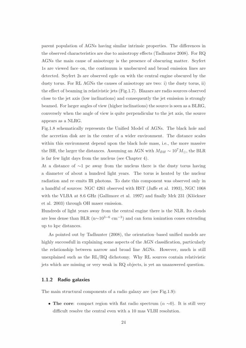
1.6 AGN 3–D classification. . . . . . . . . . . . . . . . . . . . . . . . 23
1.7 Relative inclinations of torus and jet in a RL AGN. . . . . . . . 25
1.8 Schematic representation of the Unified Model of AGNs. . . . . . 26
1.9 Cygnus A 6 cm radio map. . . . . . . . . . . . . . . . . . . . . . 28
1.10 Examples of FRI and FRII radio galaxies. . . . . . . . . . . . . . 28
1.11 Schematic representation of a rotating black hole. . . . . . . . . 31
1.12 Schematic representation of the ADAF solution. . . . . . . . . . 32
1.13 Typical ADAF spectrum. . . . . . . . . . . . . . . . . . . . . . . 33
1.14 Cartoon for the ADIOS solution . . . . . . . . . . . . . . . . . . 33
1.15 Cartoon of an ADAF plus a truncated disk. . . . . . . . . . . . . 34
1.16 Dependence of the Doppler factor on the angle to the line of sight. 35
1.17 Schematic representation of the synchrotron physical process. . . 37
1.18 Inverse Compton process. . . . . . . . . . . . . . . . . . . . . . . 37
1.19 Flux and spectral slope variations of NGC 1275. . . . . . . . . . 41
1.20 3C 120 100 MeV–100 GeV count sky map. . . . . . . . . . . . . 42
1.21 The Γ–Lγ plane. . . . . . . . . . . . . . . . . . . . . . . . . . . . 43
1.22 CD vs. total flux at 178 MHz of the 3CRR sample. . . . . . . . 44
1.23 Unfolded model of the combined XMM and Swift datasets. . . . 46
1.24 Nuclear broadband SED of NGC 6251 . . . . . . . . . . . . . . . 47
5

2.1 Cosmic elemental abundances as a function of Z. . . . . . . . . . 51
2.2 Representation of the two main radiation–driven processes. . . . 53
2.3 Radiative recombination continua (RRC) for He–like O. . . . . . 55
2.4 Fractional ionic abundances vs. ionization parameter (ξ). . . . . 57
2.5 Temperature vs the ionization parameter ξ. . . . . . . . . . . . . 58
2.6 Temperature vs the ionization parameter Ξ. . . . . . . . . . . . . 58
2.7 Ratio of higher series Ly lines to Lyα as a function of TOV III . . 60
2.8 Simplified Gotrian diagram for He–like triplets. . . . . . . . . . . 61
2.9 G ratio as a function of the electronic temperature. . . . . . . . 62
2.10 OVII(f)/OVIIILyα vs LO. . . . . . . . . . . . . . . . . . . . . . . 62
2.11 Plot of the R–ratio as a function of ne. . . . . . . . . . . . . . . 63
2.12 OVII theoretical spectra for three values of electron density. . . . 64
2.13 PI plasma where photoexcitation or collisional excitation occurred. 64
2.14 Allowed energy level and electronic transitions for a generic atom. 65
2.15 Voigt profile. . . . . . . . . . . . . . . . . . . . . . . . . . . . . . 67
2.16 First detection of iron UTA feature from Sako et al. (2001). . . . 68
3.1 Two orientations of an AGN respect the observer line–of–sight. . 70
3.2 Absorption and reemission spectra of He–like O. . . . . . . . . . 70
3.3 Radio/X–ray image on 3C 33. . . . . . . . . . . . . . . . . . . . 73
3.4 Residuals of the two soft excess models tested for 3C 33. . . . . . 78
3.5 Chandra and XMM–Newton spectra of 3C 33. . . . . . . . . . . 80
3.6 Contours plot for normalization vs centroid energy of Fe Kα line. 81
3.7 Combined Chandra, XMM and Suzaku 0.5–1.5 keV spectrum. . . 83
3.8 Chandra soft X-ray contours overlaid on an HST OIII image. . . 84
3.9 Line diagnostic diagram from Miller et al. (2003). . . . . . . . . 85
4.1 Line diagnostic diagram from Miller et al. (2003) applied to 3C 382. 90
4.2 Zoom of the 3C 382 RGS observed–frame spectra. . . . . . . . . 93
4.3 Radio to X–ray spectral energy distribution of 3C 382. . . . . . . 94
4.4 Contour plots for WA NH and ξ values obtained with the XSTAR. 94
4.5 Best fit rest–frame XSTAR model of 3C 382 in the RGS band. . 95
4.6 Spectral energy distributions (SEDs) of 3C 390.3 and 3C 120. . . 100
4.7 Zoomed region of the 3C 390.3 residuals. . . . . . . . . . . . . . 101
6

4.8 SPEX modelling of 3C 390.3 RGS spectrum . . . . . . . . . . . . 102
4.9 3C 390.3 residuals for the OVII forbidden line. . . . . . . . . . . 102
4.10 3C 120 RGS residuals. . . . . . . . . . . . . . . . . . . . . . . . . 105
5.1 Mout vs. Macc; Eout vs. Lbol. . . . . . . . . . . . . . . . . . . . . 114
5.2 Mout vs. rl; Eout vs. rl. . . . . . . . . . . . . . . . . . . . . . . . 115
6.1 10 ks XGS simulation of 3C 33. . . . . . . . . . . . . . . . . . . 121
6.2 10 ks XGS simulation 3C 382. . . . . . . . . . . . . . . . . . . . 122
A.1 Representation of the XMM–Newton orbit. . . . . . . . . . . . . 124
A.2 Sketch of the XMM–Newton payload. . . . . . . . . . . . . . . . 124
A.3 Optical system adopted for X–ray telescopes. . . . . . . . . . . . 127
A.4 Effective area of XMM–Newton X–ray telescopes. . . . . . . . . 128
A.5 Light path through the X–ray telescope. . . . . . . . . . . . . . . 128
A.6 Fractional encircled energy for pn. . . . . . . . . . . . . . . . . . 129
A.7 Fractional encircled energy for MOS. . . . . . . . . . . . . . . . . 129
A.8 FOV and CCD assembly of the EPIC cameras. . . . . . . . . . . 130
A.9 The Reflection Grating Array. . . . . . . . . . . . . . . . . . . . 133
A.10Representation of the RGS Focal Camera. . . . . . . . . . . . . . 133
A.11RGS effective area. . . . . . . . . . . . . . . . . . . . . . . . . . 134
A.12Schematic representation of the OM. . . . . . . . . . . . . . . . . 134
B.1 The Chandra satellite. . . . . . . . . . . . . . . . . . . . . . . . . 135
B.2 The High Resolution Camera (HRC). . . . . . . . . . . . . . . . 136
B.3 ACIS–I and ACIS–S configurations. . . . . . . . . . . . . . . . . 137
B.4 The Low Energy Trasmission Grating onboard Chandra . . . . . 138
B.5 The High Energy Trasmission Gratings onboard Chandra. . . . . 138
B.6 Gratings effective areas of Chandra and XMM–Newton. . . . . . 139
B.7 Grating resolving powers of Chandra and XMM–Newton. . . . . 139
C.1 The IXO satellite. . . . . . . . . . . . . . . . . . . . . . . . . . . 141
C.2 IXO instrument module. . . . . . . . . . . . . . . . . . . . . . . 142
C.3 Effective area of IXO mirror and instruments. . . . . . . . . . . 143
7

8
List of Tables
List of Tables 9
1.1 The MAGN sample. . . . . . . . . . . . . . . . . . . . . . . . . . 41
3.1 Chandra ACIS–S best–fit parameters. . . . . . . . . . . . . . . . 77
3.2 Emission lines detected in the Chandra ACIS–S spectrum. . . . . 78
3.3 XMM–Newton EPIC pn best–fit parameters. . . . . . . . . . . . 79
3.4 Emission lines detected in the XMM–Newton EPIC pn spectrum. 80
4.1 Soft X–ray absorption/emission lines in the 3C 382 RGS spectrum. 91
4.2 Best–fitting parameters for both 3C 390.3 observations. . . . . . 101
4.3 3C 390.3 OVII(f) emission line parameters for the two epochs. . . 103
4.4 3C 120 fit parameters for the two models tested. . . . . . . . . . 104
5.1 Summary of the BLRGs properties. . . . . . . . . . . . . . . . . 108
5.2 WA physical parameters for the sources of the sample. . . . . . . 110
5.3 Mout, Eout, Lacc, Macc, Pjet, ηj for BLRGs. . . . . . . . . . . . . . 112
A.1 XMM–Newton general characteristics. . . . . . . . . . . . . . . . 125
A.2 Comparison between XMM–Newton and other X–ray satellites. . 126
A.3 FOV and time resolution for different observing modes. . . . . . 131
9

10
Abstract
Massive galaxies appear to have a black hole at their center obeying the black hole
mass and velocity dispersion correlation (MBH–σ; Magorrian et al. 1998; Ferrarese
& Merritt 2000; Gebhardt et al. 2000; Tremaine et al. 2002), that simply reflects
the interplay between the BH and the surrounding environment. It is known that
massive black holes have a profound effect on the evolution of galaxies, and possibly
on their formation by regulating the amount of gas available for the star forma-
tion. However, how black hole and galaxies communicate is still an open problem,
depending on how much of the energy released interacts with the circumnuclear
matter. In the last years, most studies of feedback have primarily focused on AGN
jet/cavity systems in the most massive, X–ray luminous galaxy clusters. This thesis
intends to investigate the feedback phenomena in radio–loud AGNs from a different
perspective. Indeed it presents an X–ray study of the circumnuclear environment of
isolated powerful radio galaxies, through XMM–Newton and Chandra observations.
In particular, the high–resolution spectroscopy technique is exploited to search for
gaseous outflows in order to better understand the physical and kinematic conditions
of the gas surrounding supermassive black holes.
Specifically, one Narrow Line Radio Galaxy (3C 33) and three Broad Line Radio
Galaxies (3C 382, 3C 390.3 and 3C 120), are studied in detail, searching for warm
photoionized gas, both in emission and absorption, in the soft X–ray band (0.3–2
keV). As a result, I found that the soft X–ray spectrum of 3C 33 could originate
from gas photoionized by the central engine, rather than from the jet emerging
from the edge of the torus, as previous suggested by several authors. Moreover
the high–resolution spectra revealed for the first time the presence of soft X–ray
warm absorbers in both 3C 382 and 3C 390.3. On the contrary, no indication of
warm absorbing gas is found in 3C 120, the BLRG of the sample with the smallest
inclination angle. The observed warm absorbers have column densities, ionization
parameters and outflowing velocities in the range NH=1020−22 cm−2, logξ=2–3
11
erg cm s−1 and vout ∼102−3 km s−1, respectively. Such values constrain the location
of the gas in the Narrow Line Region, favoring a torus wind origin. The distribution
of the gas is probably not uniform. The volume filling factor has to be less than
1 otherwise the absorbers mass outflow rates turn out implausibly higher than the
mass accretion rates. However, even considering upper limits on the mass outflow
rate, the kinetic luminosity of the outflow is always well below 1% the bolometric
luminosity as well as the jet kinetic power. Finally, the radio–loud properties are
compared with those of a sample of type 1 RQ AGNs taken from the literature.
The physical parameters of radio galaxy warm absorbers are found to span a range
of values similar to Seyferts. In addition, a positive correlation is found between
the mass outflow rate/kinetic luminosity, and the radio loudness. This seems to
suggest that the presence of a radio source (the jet?) affects the distribution of the
absorbing gas, i.e., the volume filling factor. Alternatively, if the gas distribution is
similar in Seyferts and radio galaxies, the Mout vs rl relation could simply indicate
a major ejection of matter in the form of wind in powerful radio AGNs.
The chapters of this thesis are organized as follows:
• Chapter 1 gives an overview of the general properties of AGNs, mainly focused
on radio–loud sources which are the subject of this study. Their radio, optical
and X–ray spectral characteristics are fully described, and the very recent
Fermi–LAT results on non–blazar AGNs are also reported.
• Chapter 2 provides basic physical notions necessary for the interpretation of
high–resolution X–ray spectra. The atomic transitions, and in particular the
radiation–driven processes are described, together with the most important
line diagnostics for a photoionized gas.
• Chapter 3 presents the analysis and results obtained from the XMM–Newton
and Chandra observations of the NLRG 3C 33. In particular, photoionized
gas in emission is invoked to explain the soft excess in the spectrum.
• Chapter 4 describes the high–resolution analysis performed on three BLRGs.
As a result, the detection of warm absorber was obtained for the first time in
two of such objects.
• Chapter 5 compares the previously found properties of BLRG warm absorbers
with a sample of type 1 RQ AGNs as taken from the literature. The main
result is the correlation found between the mass outflow rate (and the kinetic
luminosity of the outflow) and the radio loudness parameter.
12

• Discussions and conclusions are presented in Chapter 6.
• The Appendices report general information on the X–ray satellites used through-
out this thesis.
13

14
1Introduction
1.1 Active Galactic Nuclei
Active Galactic Nuclei (AGNs) are among the most powerful sources of electromag-
netic radiation in the Universe. They produce enormous luminosities (from 1042 to
1048 erg s−1) in very small volumes (probably <<1 pc3).
AGNs emit their power in the overall electromagnetic spectrum, from radio to
gamma–rays, forming the so called Spectral Energy Distribution, or SED (Fig.1.1),
in which different processes inside and outside the active nucleus are present.
• Radio: radio waves have a non–thermal origin. They are emitted through
synchrotron radiation produced by relativistic electrons spiraling in a mag-
netic field. Electrons are forced to change direction and, as a result, they are
accelerated and radiate electromagnetic energy. The frequency of the emit-
ted radiation depends on the magnetic field strength and on the energy of
the electrons (see Section 1.2.2). Radio–loud AGNs are powerful radio emit-
ters because relativistic electrons in the jets emit synchrotron radiation (see
Section 1.2.2). Conversely, radio–quiet AGNs emit weak or null radio waves.
• Infrared: the IR band contains re–emission from hot dust nearby the active
nucleus, that has been heated by the central engine. Therefore, at least around
1–40 µm, the reprocessed nuclear optical/UV/X–ray light is dominant. Three
pieces of evidence support the thermal origin (Peterson 1997).
i) The 1 µm minimum is a general feature in the SED of AGNs (Sanders et
15
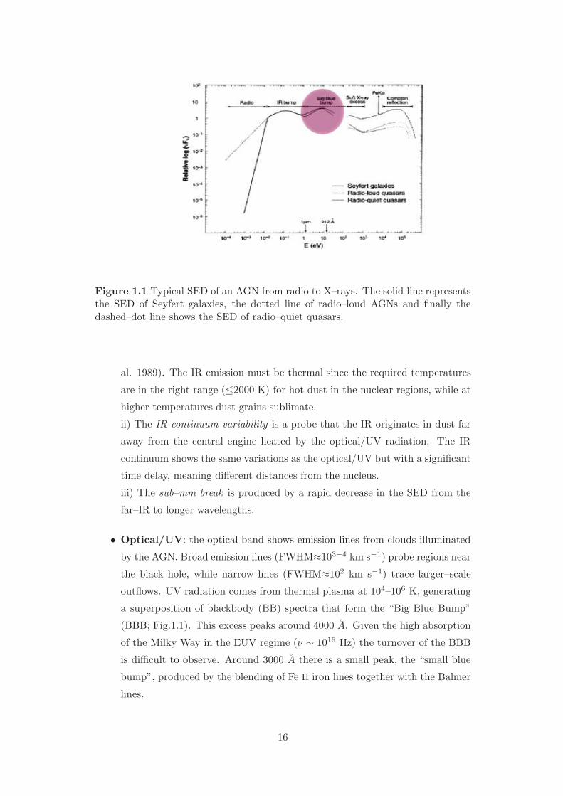
Figure 1.1 Typical SED of an AGN from radio to X–rays. The solid line representsthe SED of Seyfert galaxies, the dotted line of radio–loud AGNs and finally thedashed–dot line shows the SED of radio–quiet quasars.
al. 1989). The IR emission must be thermal since the required temperatures
are in the right range (≤2000 K) for hot dust in the nuclear regions, while at
higher temperatures dust grains sublimate.
ii) The IR continuum variability is a probe that the IR originates in dust far
away from the central engine heated by the optical/UV radiation. The IR
continuum shows the same variations as the optical/UV but with a significant
time delay, meaning different distances from the nucleus.
iii) The sub–mm break is produced by a rapid decrease in the SED from the
far–IR to longer wavelengths.
• Optical/UV: the optical band shows emission lines from clouds illuminated
by the AGN. Broad emission lines (FWHM≈103−4 km s−1) probe regions near
the black hole, while narrow lines (FWHM≈102 km s−1) trace larger–scale
outflows. UV radiation comes from thermal plasma at 104–106 K, generating
a superposition of blackbody (BB) spectra that form the “Big Blue Bump”
(BBB; Fig.1.1). This excess peaks around 4000 A. Given the high absorption
of the Milky Way in the EUV regime (ν ∼ 1016 Hz) the turnover of the BBB
is difficult to observe. Around 3000 A there is a small peak, the “small blue
bump”, produced by the blending of Fe II iron lines together with the Balmer
lines.
16
The following wavebands are also called high–energy regimes. They are of
great importance to understand the AGN phenomenon and constitute the
central part of this thesis.
• X–ray: X–rays (0.1–200 keV) account for ∼ 10% of the AGN bolometric
luminosity. They can vary rapidly, suggesting an origin in the innermost re-
gions of the active nucleus. The most popular model, invoked to explain
these phenomena, involves accretion onto black holes, i.e. conversion of the
gravitational energy of accreting material into electromagnetic radiation, as
indipendently argued by Salpeter (1964) and Zeldovich (1964).
Twenty years later, Rees (1984) theorized this phenomenon involving the ac-
cretion of matter onto a Supermassive Black Hole (SMBH), whose mass can
be up to 109 M⊙. Before accreting, the matter loses its angular momentum
and forms a disk around the black hole that emits blackbody (BB) radiation in
the UV band. The BB temperature decreases as the distance increases, thus
the outer part of the disk, few light days across, emits in the optical regime.
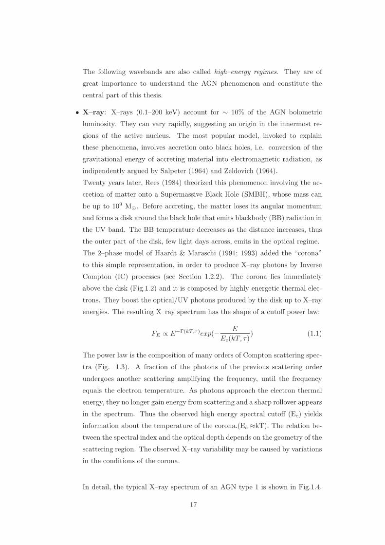
The 2–phase model of Haardt & Maraschi (1991; 1993) added the “corona”
to this simple representation, in order to produce X–ray photons by Inverse
Compton (IC) processes (see Section 1.2.2). The corona lies immediately
above the disk (Fig.1.2) and it is composed by highly energetic thermal elec-
trons. They boost the optical/UV photons produced by the disk up to X–ray
energies. The resulting X–ray spectrum has the shape of a cutoff power law:
FE ∝ E−Γ(kT,τ)exp(−E
Ec(kT, τ)) (1.1)
The power law is the composition of many orders of Compton scattering spec-
tra (Fig. 1.3). A fraction of the photons of the previous scattering order
undergoes another scattering amplifying the frequency, until the frequency
equals the electron temperature. As photons approach the electron thermal
energy, they no longer gain energy from scattering and a sharp rollover appears
in the spectrum. Thus the observed high energy spectral cutoff (Ec) yields
information about the temperature of the corona.(Ec ≈kT). The relation be-
tween the spectral index and the optical depth depends on the geometry of the
scattering region. The observed X–ray variability may be caused by variations
in the conditions of the corona.
In detail, the typical X–ray spectrum of an AGN type 1 is shown in Fig.1.4.
17

Figure 1.2 Schematic representation adapted from Haardt, Maraschi & Ghisellini(1994) of the 2–phase model. The accretion disk lies very close to the BH. It isthe region where UV/soft–X–ray photons are produced. Successively, they are up–scattered by the hot corona through thermal Comptonization. In this sketch anaccretion disk wind (warm absorber) is also represented.
Figure 1.3 Example of a power law continuum as a result of the superposition ofmany orders of Compton scattering spectra. From Ghisellini lessons, September 13,2008.
18

I will briefly describe the most important features.
1. The soft excess (E<1 keV) is observed in many AGNs and its origin is
not clear. It has been argued that it is the Comptonized Wien tail of the
BBB, however this seems to be unlikely because it would require TBBB ∼2 × 10⁵ K, too high for an accretion disk (for more details see Section
1.2.1). Moreover this component shows a fixed temperature around 0.2
keV indipendently on the BH mass. This constancy of the temperature
indicates a relation between soft excess and atomic transitions (Netzer
1996; Gierlinski & Done (2004).
An alternative interpretation of the soft excess was involves the warm
absorber.
2. The warm absorber is a recurrent characteristic in Seyfert 1 galaxies
(see Chapter 4), e.g. face–on AGNs. It is ionized gas, positioned along
the line–of–sight, that absorbs the nuclear radiation, hence producing
absorption lines over the soft X–ray and UV continua. It is generally
characterized by a large range of ionization parameters, ξ (ξ = LnR2 , for
more details see Chapter 2), and column densities, NH , and typically it
is outflowing at velocities ranging from several hundreds to thousands
km s−1, depending on where this wind is launched.
3. The Fe Kα line is produced by fluorescence (see Chapter 2). When the
lines are produced very close to the BH, they are shaped by the effects
of Doppler shifts and gravitational effects (see Fig.1.5). Narrow lines can
be produced in the BLR and in the torus.
4. The reflection hump: half of the X–rays escape from the corona and are
reflected back to the accretion disk, producing the reflection component
(Fig.1.4) which can give rise to the “Compton hump” peaking at 20–50
keV.
• Gamma–rays: γ–rays (E>100 MeV) have the smallest wavelength and the
greatest energy of any other waveband. In this regime non–thermal processes
dominate and it is possible to study the behaviour of some of the most ener-
getic and extreme objects in the Universe (see also Section 1.3).
There are several important mechanisms producing γ-rays in astrophysical
objects. Among them there is the IC scattering (Fig.1.18). This process takes
place when high–energy relativistic electrons scatter low energy photons to
19
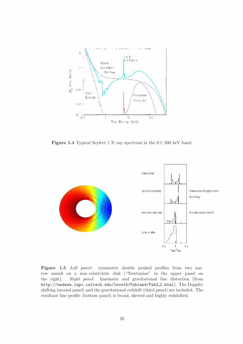
Figure 1.4 Typical Seyfert 1 X–ray spectrum in the 0.1–200 keV band.
Figure 1.5 Left panel : symmetric double peaked profiles from two nar-row annuli on a non–relativistic disk (“Newtonian” in the upper panel onthe right). Right panel : kinematic and gravitational line distortion (fromhttp://nedwww.iapc.caltech.edu/level5/Fabian4/Fab2 2.html). The Dopplershifting (second panel) and the gravitational redshift (third panel) are included. Theresultant line profile (bottom panel) is broad, skewed and highly redshifted.
20

higher energies (e.g. in the jets). The frequency of the up–scattered photons
is proportional to γ2eν where γe is the Lorentz factor of the electron, and ν is
the initial photon frequency.
1.1.1 AGN classification and the Unified Model
AGNs emit over the entire electromagnetic spectrum, consequently they were discov-
ered and classified separately at different wavelenghts. Therefore the classification
of AGNs is complex and employes many different methods (Tadhunter 2008) such
as the presence or absence of broad emission lines in the optical spectra, the optical
morphology, the radio morphology, the variability, the luminosity or the spectral
shape.
Another important property is the radio loudness. An object is defined “radio–loud”
(RL) if the ratio between the radio emission at 5 GHz and the optical flux in the B
band is equal or higher than 10 (Kellermann et al. 1989):
F5GHz
FB≥ 10 (1.2)
otherwise the object is called “radio–quiet” (RQ).
A more recent definition of radio loudness was introduced by Terashima & Wilson
(2003):
RX =νLν(5GHz)
LX(1.3)
where LX is the unabsorbed luminosity in the 2–10 keV band. The advantage with
respect to the usual definition is that RX can be applied to heavily obscured nuclei
(NH ≥1023 cm−2, AV >50 mag).
Only a small fraction (15–20 %) of AGNs is RL (Urry & Padovani 1995).
RQ AGNs lie generally in spiral galaxies (Floyd et al. 2004) while RL AGNs are
hosted exclusively in elliptical galaxies. Antonucci (2011) shows that, in the low–z
Universe, there is a near–perfect correspondence between RL objects and elliptical
hosts.
The very first classification of AGNs was made in the optical band on the basis
of the presence and relative strength of emission lines. This classification can be
adopted for both RL and RQ sources (Fig.1.6):
- Type I AGNs: they are characterized by a bright continuum and strong
broad (permitted) and narrow (forbidden) emission lines. Broad lines (FWHM≈
21

several 103−4 km s−1) are produced by clouds of hot gas near the BH (<1 pc),
in the Broad Line Regions (BLR), while the narrow lines (FWHM≈ 102 km s−1)
are emitted far from the BH in the Narrow Line Regions (NLR). RQ sources
belonging to this class are Seyfert 1s and RQ QSOs, while RL sources are
Broad Line Radio Galaxies (BLRG), Steep Spectrum Radio Quasars (SSRQ)
and Flat Spectrum Radio Quasars (FSRQ). Few high–luminosity AGNs show-
ing broad optical/UV absorption lines are called BAL QSOs.
- Type II AGNs: they show a weaker continuum and only narrow emission
lines. A possible explanation for the lack of broad lines is that either the BLR
are missing or, most likely, the central engine is obscured by an intervening
medium, i.e. the dusty torus. RQ sources are Seyfert 2s, and RL sources
are High Excitation Galaxies (HEG; Jackson & Rawlings 1997) Narrow Line
Radio Galaxies (NLRG).
- LINERs: at the lower end of the luminosity scale there are the Low–Ionization
Nuclear Emission–Line Region galaxies (Heckman, 1980) with the continuum
dominated by the host galaxy. Spectroscopically they resemble Seyfert 2s, ex-
cept that the low–ionization lines, (e.g., [OI]λ6300, [NII]λλ6548,6583) are rela-
tively strong. RL AGNs, similar to LINERs, are the Weak Line Radio Galaxies
(WLRG), also called Low Excitation Galaxies (LEG). They are characterized
by low EW (<10 A ; Tadhunter et al. 1998) or [OII]/[OIII]>1 (Jackson &
Rawlings 1997) and low ionization.
- BL Lac objects: the spectrum is dominated by non–thermal continuum
emission and no, or weak, emission lines (EW<5 A ) are present. Together
with FSRQs, BL Lac objects form the Blazars class. These sources are viewed
nearly along the jet axis, therefore the non–thermal jet radiation is amplified
by relativistic effects giving rise to flat radio spectra, large polarization and
strong variability. Blazars generally show two–peaked broad–band SEDs from
radio to γ–rays. Synchrotron radiation forms the lower–energy part of the
SED from radio to optical/UV. Sometimes it can extends up to the X–ray
band. The Compton processes make the X–ray/γ–ray radiation. Blazars are
the largest population of AGNs observed in the γ–ray sky (Hartman et al.
1999; Abdo et al. 2010a,b).
The Unified Model (Antonucci 1993; Urry & Padovani 1995) explains the variety
of AGNs in terms of orientation, i.e., different AGN types all belong to the same
22
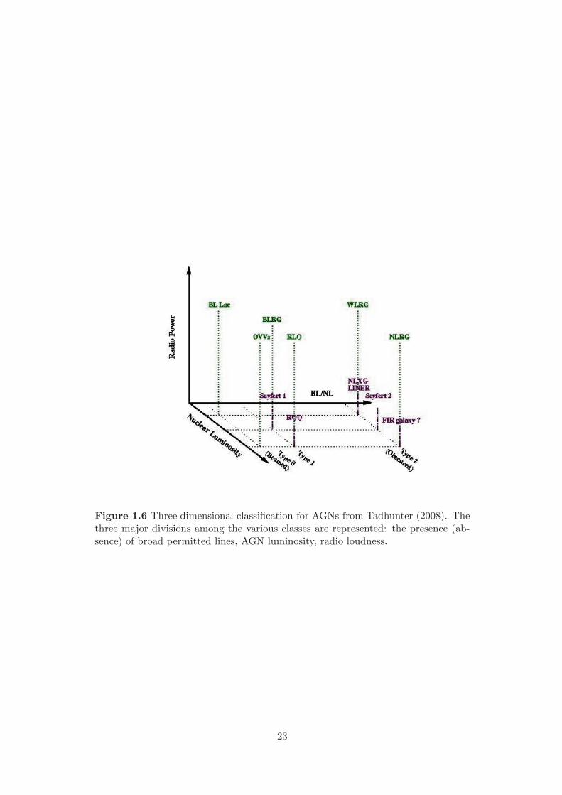
Figure 1.6 Three dimensional classification for AGNs from Tadhunter (2008). Thethree major divisions among the various classes are represented: the presence (ab-sence) of broad permitted lines, AGN luminosity, radio loudness.
23
parent population of AGNs having similar intrinsic properties. The differences in
the observed characteristics are due to anisotropy effects (Tadhunter 2008). For RQ
AGNs the main cause of anisotropy is the presence of obscuring matter. Seyfert
1s are viewed face–on, the continuum is unobscured and broad emission lines are
detected. Seyfert 2s are observed egde–on with the central engine obscured by the
dusty torus. For RL AGNs the causes of anisotropy are two: i) the dusty torus, ii)
the effect of beaming in relativistic jets (Fig.1.7). Blazars are radio sources observed
close to the jet axis (low inclinations) and consequently the jet emission is strongly
beamed. For larger angles of view (higher inclinations) the source is seen as a BLRG,
conversely when the angle of view is quite perpendicular to the jet axis, the source
appears as a NLRG.
Fig.1.8 schematically represents the Unified Model of AGNs. The black hole and
the accretion disk are in the center of a wider environment. The distance scales
within this environment depend upon the black hole mass, i.e., the more massive
the BH, the larger the distances. Assuming an AGN with MBH ∼ 107M⊙, the BLR
is far few light days from the nucleus (see Chapter 4).
At a distance of ∼1 pc away from the nucleus there is the dusty torus having
a diameter of about a hundred light years. The torus is heated by the nuclear
radiation and re–emits IR photons. To date this component was observed only in
a handful of sources: NGC 4261 observed with HST (Jaffe et al. 1993), NGC 1068
with the VLBA at 8.6 GHz (Gallimore et al. 1997) and finally Mrk 231 (Klockner
et al. 2003) through OH maser emission.
Hundreds of light years away from the central engine there is the NLR. Its clouds
are less dense than BLR (n∼103−6 cm−3) and can form ionization cones extending
up to kpc distances.
As pointed out by Tadhunter (2008), the orientation–based unified models are
highly successfull in explaining some aspects of the AGN classification, particularly
the relationship between narrow and broad line AGNs. However, much is still
unexplained such as the RL/RQ dichotomy. Why RL sources contain relativistic
jets which are missing or very weak in RQ objects, is yet an unanswered question.
1.1.2 Radio galaxies
The main structural components of a radio galaxy are (see Fig.1.9):
• The core: compact region with flat radio spectrum (α ∼0). It is still very
difficult resolve the central even with a 10 mas VLBI resolution.
24

Figure 1.7 The causes of anisotropy in a RL AGN are two, the torus and the jet.As shown in this sketch, the relative disk–jet strength depends on the viewing angle.When the jet is pointing at large angles (θ ≥45) with respect to the observer line–of–sight, the disk is completely hidden by the circumnuclear torus and the objectis classified as NLRG. If the jet is pointing closer to the line–of–sight, the AGNbecomes directly visible and it is classified as quasar or as BLRG. At even smallerangles the AGN spectrum is dominated by the inner jet emission, and the objectis classified as a FSRQ. The left column shows how the host galaxy appears fordifferent inclination angles of the jet.
25
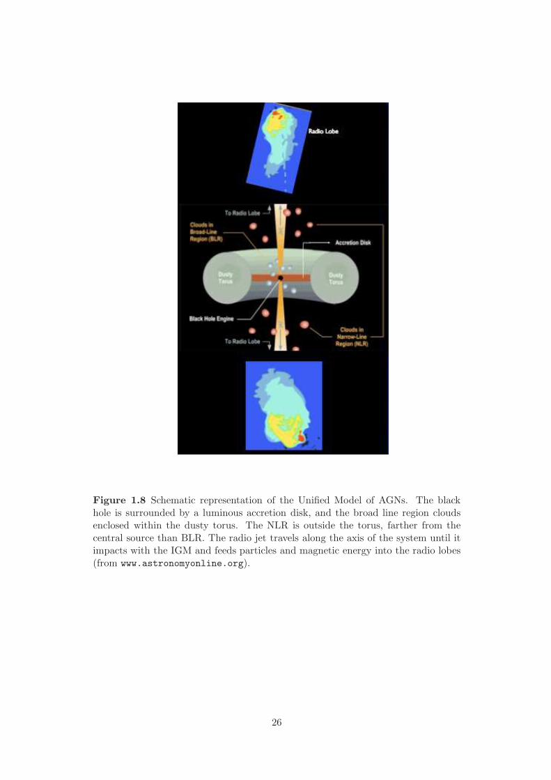
Figure 1.8 Schematic representation of the Unified Model of AGNs. The blackhole is surrounded by a luminous accretion disk, and the broad line region cloudsenclosed within the dusty torus. The NLR is outside the torus, farther from thecentral source than BLR. The radio jet travels along the axis of the system until itimpacts with the IGM and feeds particles and magnetic energy into the radio lobes(from www.astronomyonline.org).
26
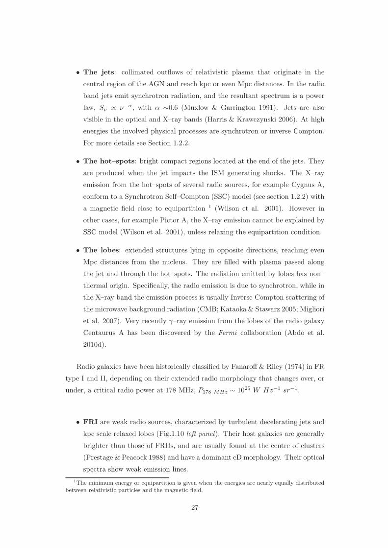
• The jets: collimated outflows of relativistic plasma that originate in the
central region of the AGN and reach kpc or even Mpc distances. In the radio
band jets emit synchrotron radiation, and the resultant spectrum is a power
law, Sν ∝ ν−α, with α ∼0.6 (Muxlow & Garrington 1991). Jets are also
visible in the optical and X–ray bands (Harris & Krawczynski 2006). At high
energies the involved physical processes are synchrotron or inverse Compton.
For more details see Section 1.2.2.
• The hot–spots: bright compact regions located at the end of the jets. They
are produced when the jet impacts the ISM generating shocks. The X–ray
emission from the hot–spots of several radio sources, for example Cygnus A,
conform to a Synchrotron Self–Compton (SSC) model (see section 1.2.2) with
a magnetic field close to equipartition 1 (Wilson et al. 2001). However in
other cases, for example Pictor A, the X–ray emission cannot be explained by
SSC model (Wilson et al. 2001), unless relaxing the equipartition condition.
• The lobes: extended structures lying in opposite directions, reaching even
Mpc distances from the nucleus. They are filled with plasma passed along
the jet and through the hot–spots. The radiation emitted by lobes has non–
thermal origin. Specifically, the radio emission is due to synchrotron, while in
the X–ray band the emission process is usually Inverse Compton scattering of
the microwave background radiation (CMB; Kataoka & Stawarz 2005; Migliori
et al. 2007). Very recently γ–ray emission from the lobes of the radio galaxy
Centaurus A has been discovered by the Fermi collaboration (Abdo et al.
2010d).
Radio galaxies have been historically classified by Fanaroff & Riley (1974) in FR
type I and II, depending on their extended radio morphology that changes over, or
under, a critical radio power at 178 MHz, P178 MHz ∼ 1025 W Hz−1 sr−1.
• FRI are weak radio sources, characterized by turbulent decelerating jets and
kpc scale relaxed lobes (Fig.1.10 left panel). Their host galaxies are generally
brighter than those of FRIIs, and are usually found at the centre of clusters
(Prestage & Peacock 1988) and have a dominant cD morphology. Their optical
spectra show weak emission lines.
1The minimum energy or equipartition is given when the energies are nearly equally distributedbetween relativistic particles and the magnetic field.
27
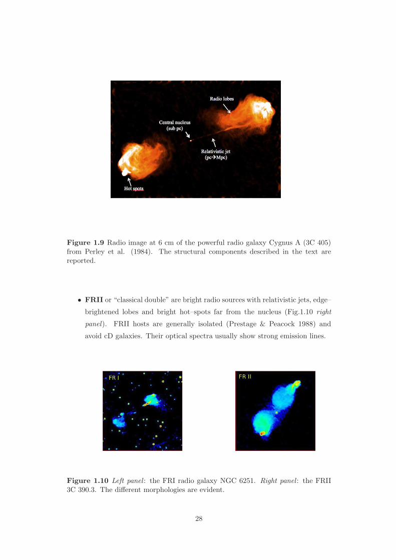
Figure 1.9 Radio image at 6 cm of the powerful radio galaxy Cygnus A (3C 405)from Perley et al. (1984). The structural components described in the text arereported.
• FRII or “classical double” are bright radio sources with relativistic jets, edge–
brightened lobes and bright hot–spots far from the nucleus (Fig.1.10 right
panel). FRII hosts are generally isolated (Prestage & Peacock 1988) and
avoid cD galaxies. Their optical spectra usually show strong emission lines.
Figure 1.10 Left panel : the FRI radio galaxy NGC 6251. Right panel : the FRII3C 390.3. The different morphologies are evident.
28
Two accredited hypothesis try to explain the different radio morphology of FRIs
and FRIIs: 1) the interplay between the jet energy and the density of the environ-
ment; in this scenario FRIs and FRIIs are different manifestations of the same
phenomenon. 2) Different accretion modes onto the SMBH; for FRIIs a standard
Shakura & Sunyaev (1973) radiatively efficient accretion disk is invoked (see Sec-
tion 1.4), instead for FRIs low accretion rates and low radiation efficiencies (ADAF,
ADIOS,...) are proposed. The transition from FRIs to FRIIs would be due to a
change in the accretion mode and can be related to an evolutionary scenario (Ghis-
ellini & Celotti 2001; Marchesini et al. 2004). It is possible that all AGNs pass
through a jet phase (FRII), then when the accreted gas is exhausted the AGN turns
into low–power FRIIs and successively FRIs.
In a very recent review, Antonucci (2011) divides radio galaxies in thermal and
non–thermal sources depending on their accretion modes. Thermal RGs contain
hidden (by the torus) quasar nuclei, while non–thermal ones are weakly accreting
galaxies (but powerful synchrotron emitters) characterized by weak low–ionization
lines.
Besides FRIs and FRIIs, there is also another class of objects, the Compact
Sources, that are powerful radio emitters peaking at MHz–GHz frequencies. They
are very small, generally in the size range 1–20 kpc, i.e., smaller than typical host
galaxies. To date there are two possible explanations for their compactness: i)
they are young AGNs in expansion through interactions with the ISM, and this is
supported by estimates on the jets ages around 104–106 yr through VLBI proper
motions (Giroletti 2008); ii) they are frustated AGNs confined by the ISM and so
not evolved in full–size AGNs. However, this latter scenario is less plausible since
the densities and properties of the surrounding gas are comparable with those in
extended AGNs (O’Dea 1998). There are two main types of compact sources: the
Compact Steep–Spectrum (CSS) sources and the Gigahertz Peaked Spectrum (GPS)
sources. CSS are miniature classical double radio galaxies with more pronounced
asymmetries. They are extended on kpc scales with an estimated age around 106 yr
and have steep spectra (α >0.5). GPS are powerful radio sources, peaking at GHz
frequencies (smaller galaxies peak at higher frequencies). They are smaller than
CSS, infact their extension is contained within the NLR (≤1 pc).
Finally, RL quasars are subdivided into two different groups depending if they are
steep radio spectrum dominated (SSRQs, αr >0.5) or flat radio spectrum dominated
(FSRQs, αr >0.5). SSRQs tend to have lobe–dominated radio morphologies, while
29
FSRQs often have core–dominated radio structures and are highly variable.
1.2 Accretion and jet link
A common characteristic that is shared by all radio–loud AGNs is the presence of
two competitive components, the disk and the jet, which are usually mixed when
arrive to the observer. Although in some cases one component dominates over
the other one (e.g., in Blazars the jet radiation is dominant), generally the resultant
spectrum is a combination of both and the challenge is to distinguish between them.
1.2.1 Accretion
Black holes aggregate matter from their surroundings through accretion. The effi-
ciency of this process is measured in terms of the released luminosity
Lacc = ηMc2 (1.4)
where η is the efficiency of conversion of the rest mass energy of the accreting
material into radiation, and M is the accretion rate in M⊙ yr−1.
Differently from other astrophysical objects like the stars, accreted matter falling
into the black hole after crossing the Schwarschild radius (or event horizon) 2 cannot
escape anymore (Fig.1.11). The Schwarschild radius is defined as:
RS =2GM
c2∼ 3 × 10¹³ M8 cm (1.5)
Another important quantity that must be considered when dealing with AGNs,
is the Eddington luminosity (LE). LE is the luminosity at which the outward force
of the radiation pressure is balanced by the inward gravitational force:
LE =4πGmpcM
σT∼ 1.3 × 1038(M/M⊙) erg s−1 (1.6)
Accretion processes involve rotating gas flow. To determine the accretion flow
structure is necessary to solve simultaneously four conservative equations:
2According to the Penrose process it is possible to extract energy from a rotating BH becausethe rotational energy of the BH is located outside the event horizon, precisely in the ergosphere. Inthe process, the BH loses part of its angular momentum that is converted into exctracted energy.
30

Figure 1.11 Schematic representation of a rotating black hole with the two relevantsurfaces: the spherical event horizon and the oblate ergosphere. Within the ergo-sphere the spacetime is dragged along in the direction of the BH rotation at a speedgreater than the speed of light. Since the ergosphere is located outside the eventhorizon, the Penrose process theorized that it is still possible to exctract energy froma rotating BH.
1. conservation of vertical momentum
2. conservation of mass
3. conservation of energy
4. conservation of angular momentum
There are four different solutions to these equations and consequently four mod-
els. The most famous are: the Shakura & Sunyaev (1973) geometrically thin opti-
cally thick accretion disk, or the standard model, and the optically thick advection
dominated accretion flow, or ADAF (Ichimaru 1977; Narayan & Yi 1994; 1995;
Abramowicz et al. 1995). Both solutions invoke viscosity as the source of heat that
is radiated away. It transports angular momentum outward allowing the accretion
gas to spiral toward the black hole.
• In the standard model (Shakura & Sunyaev 1973) the local emission of the
disk can be approximated to a blackbody. The effective temperature (Teff)
of the photosphere is:
Teff (r) ∼ 6.3 × 10⁻⁵(M
ME
)1/4M−1/48 (
r
RS)−3/4K (1.7)
31
For an AGN with MBH=108 M⊙, Teff is in the range 105–107 K and the peak
occurs at UV–soft–X–ray region (the Big Blue Bump), νmax=2.8kT/h∼1016 Hz.
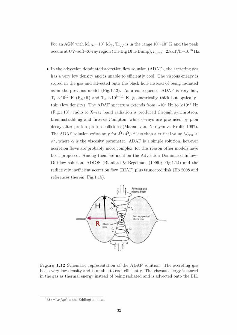
• In the advection dominated accretion flow solution (ADAF), the accreting gas
has a very low density and is unable to efficiently cool. The viscous energy is
stored in the gas and advected onto the black hole instead of being radiated
as in the previous model (Fig.1.12). As a consequence, ADAF is very hot,
Ti ∼1012 K (RS/R) and Te ∼109−11 K, geometrically–thick but optically–
thin (low density). The ADAF spectrum extends from ∼109 Hz to ≥1023 Hz
(Fig.1.13): radio to X–ray band radiation is produced through synchrotron,
bremmstrahlung and Inverse Compton, while γ–rays are produced by pion
decay after proton–proton collisions (Mahadevan, Narayan & Krolik 1997).
The ADAF solution exists only for M/ME3 less than a critical value Mcrit <
α2, where α is the viscosity parameter. ADAF is a simple solution, however
accretion flows are probably more complex, for this reason other models have
been proposed. Among them we mention the Advection Dominated Inflow–
Outflow solution, ADIOS (Blanford & Begelman (1999); Fig.1.14) and the
radiatively inefficient accretion flow (RIAF) plus truncated disk (Ho 2008 and
references therein; Fig.1.15).
Figure 1.12 Schematic representation of the ADAF solution. The accreting gashas a very low density and is unable to cool efficiently. The viscous energy is storedin the gas as thermal energy instead of being radiated and is advected onto the BH.
3ME=LE/ηc2 is the Eddington mass.
32
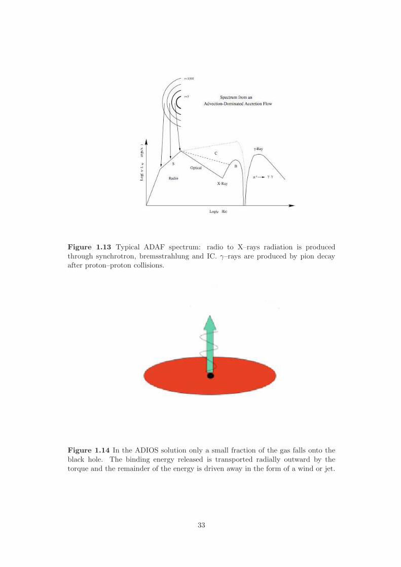
Figure 1.13 Typical ADAF spectrum: radio to X–rays radiation is producedthrough synchrotron, bremsstrahlung and IC. γ–rays are produced by pion decayafter proton–proton collisions.
Figure 1.14 In the ADIOS solution only a small fraction of the gas falls onto theblack hole. The binding energy released is transported radially outward by thetorque and the remainder of the energy is driven away in the form of a wind or jet.
33
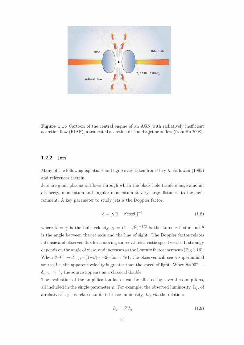
Figure 1.15 Cartoon of the central engine of an AGN with radiatively inefficientaccretion flow (RIAF), a truncated accretion disk and a jet or ouflow (from Ho 2008).
1.2.2 Jets
Many of the following equations and figures are taken from Urry & Padovani (1995)
and references therein.
Jets are giant plasma outflows through which the black hole tranfers huge amount
of energy, momentum and angular momentum at very large distances to the envi-
ronment. A key parameter to study jets is the Doppler factor:
δ = [γ(1 − βcosθ)]−1 (1.8)
where β = vc is the bulk velocity, γ = (1 − β2)−1/2 is the Lorentz factor and θ
is the angle between the jet axis and the line of sight. The Doppler factor relates
intrinsic and observed flux for a moving source at relativistic speed v=βc. It stronlgy
depends on the angle of view, and increases as the Lorentz factor increases (Fig.1.16).
When θ=0 → δmax=(1+β)γ ∼2γ for γ ≫1, the observer will see a superluminal
source, i.e, the apparent velocity is greater than the speed of light. When θ=90 →δmin=γ−1, the source appears as a classical double.
The evaluation of the amplification factor can be affected by several assumptions,
all included in the single parameter ρ. For example, the observed luminosity, Lj , of
a relativistic jet is related to its intrinsic luminosity, Lj , via the relation:
Lj = δρLj (1.9)
34
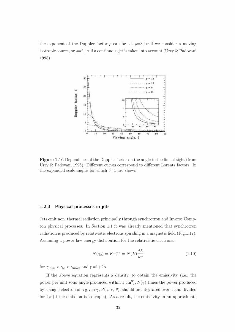
the exponent of the Doppler factor ρ can be set ρ=3+α if we consider a moving
isotropic source, or ρ=2+α if a continuous jet is taken into account (Urry & Padovani
1995).
Figure 1.16 Dependence of the Doppler factor on the angle to the line of sight (fromUrry & Padovani 1995). Different curves correspond to different Lorentz factors. Inthe expanded scale angles for which δ=1 are shown.
1.2.3 Physical processes in jets
Jets emit non–thermal radiation principally through synchrotron and Inverse Comp-
ton physical processes. In Section 1.1 it was already mentioned that synchrotron
radiation is produced by relativistic electrons spiraling in a magnetic field (Fig.1.17).
Assuming a power law energy distribution for the relativistic electrons:
N(γe) = Kγ−pe = N(E)
dE
dγ(1.10)
for γmin < γe < γmax and p=1+2α.
If the above equation represents a density, to obtain the emissivity (i.e., the
power per unit solid angle produced within 1 cm3), N(γ) times the power produced
by a single electron of a given γ, P(γ, ν, θ), should be integrated over γ and divided
for 4π (if the emission is isotropic). As a result, the emissivity in an approximate
35
range of frequencies is obtained:
ǫsin(ν) ∝ KBα+1ν−α [erg cm−3 s−1 sr−1
] (1.11)
Notice that the value p=1+2α derives from the fact that a power law electron
distribution produces a power law spectrum and the two spectral indices (α and p)
are related (Rybicki & Lightman 1979).
Inverse Compton (IC) generates when the electron energy is greater than the
photon one, and a transfer of energy from the electron to the photon can occurr
(Fig.1.18). There is a strong link between the scattered frequency νc and the electron
energy producing it:
νc =4
3γ2ν0 (1.12)
The IC emissivity (ǫc) can be deduced in the same way of the synchrotron emissivity
(ǫsin) assuming a power law distribution for the relativistic electrons (eq. 1.9). It
is possible to derive the emissivity that is again a power law, with the same link
between α and p, α=(p-1)/2:
ǫc(νc) ∝ Kν−αc
∫Ur(ν)να
νdν [erg cm−3 s−1 sr
−1] (1.13)
where Ur(ν) is the specific radiation energy density describing the upscattered pho-
ton field. When the same electrons producing synchrotron radiation are scattered,
the resultant process is called Synchrotron–Self Compton (SSC), while when the
scattered (Ur(ν)∝ ν−α) photons come from external regions like the disk or the
BLR, the torus, the NLR, the process is called External Compton (EC). The Cos-
mic Microwave Background (CMB) can be also the “seed” photons for the IC in
jets or lobes.
1.2.4 Jet orientation
The jet inclination angle is a fundamental (but difficult to constrain) parameter to
understand the physical properties of relativistic sources. It can be estimated by
different observational quantities:
• the jet/counterjet ratio, J=(1+βcosθ1−βcosθ )ρ, again ρ=2+α for a continuous jet, and
ρ=3+α if a moving isotropic source is adopted;
• the VLBI apparent velocity βa = vac of the jet knots that is related to β and
36

Figure 1.17 Schematic representation of the synchrotron physical process.
Figure 1.18 Representation of the Inverse Compton process.
37
θ via βa = βsinθ1−βcosθ (Urry & Padovani 1995);
• the general correlation between the radio core power at 5 GHz (Pc) and the
total power (Ptot) at 408 MHz in radio galaxies found by Giovannini et al.
(1988; 2001). This relation LogPc= 0.62 LogPtot+7.6 (i), obtained using a
large sample of radio galaxies selected at low frequency and therefore with
jet directions uniformly distributed in the space, corresponds to the average
orientation angle (60) with respect to the line–of–sight. Considering that the
radio core power of a source oriented at an angle θ is amplified by a quantity
Pc=Pi (1-β cos θ)−(2+α) (ii), where Pi is the intrinsic power and α is the core
radio spectral index , combining (i) and (ii) can be easily derived the relation
β = (k−1)(kcosθ−0.5) that allows to directly express β as a function of θ;
• a less robust but useful indicator of the jet orientation is the core dominance
CD=Log( Score
Stot−Score) (Scheuer & Readhead 1979), where Score (Stot) is the core
(total) flux density referred to the source rest–frame.
1.3 Radio Loud AGNs in the Fermi era
The γ–ray satellite Fermi, launched on June 2008, has shown that non–blazar (i.e.
misaligned) AGNs can be GeV emitters. With the term misaligned AGNs (MAGNs)
we define radio–loud sources whose jet is pointed away from the observer, i.e., with-
out strong Doppler boosting, with steep radio spectra (αr >0.5) and resolved and
possibly symmetrical radio structures. Given the large inclination angle of the jet,
MAGNs were not considered possible GeV emitters, but the Fermi Large Area Tele-
scope (LAT; Atwood et al. 2009) detection of 11 MAGNs in 15 months has changed
this view and confirmed MAGNs as a new an interesting class of γ–ray emitters.
Note that three MAGNs have been also discovered in the TeV band: M87 (Aha-
ronian et al. 2003), Centaurus A (Aharonian et al. 2009), NGC 1275 (Mariotti et
a. 2010). In this part of the thesis I briefly report on the recent Fermi results dec-
scribed in the papers Abdo et al. (2010c; Contact authors: P. Grandi, G. Malaguti,
G. Tosti, C. Monte) and Migliori, Grandi, Torresi et al. (2011). I was involved in
these works as an affiliated member of the Fermi–LAT collaboration.
38
1.3.1 Misaligned AGNs as a new class of GeV emitters
In 15 months, the Fermi LAT telescope could detect 11 MAGNs, all belonging to
the flux limited catalogues 3CR (Bennett 1962; Spinrad et al. 1985), 3CRR (Laing
et al. 1983) and the Molonglo Southern 4 Jy sample (MS4; Burgess & Hunstead
2006a,b).
Spectral analysis
For each source the LAT data collected from August 4, 2008 to November 8, 2009
were analyzed using the standard Fermi–LAT Science Tools software package. The
spectral study was performed using the unbinned maximum–likelihood analysis in
the gtlike tool which provides the best–fit parameters for each source.
The likelihood L is the probability of obtaining the observed data given an input
model (i.e. the distribution of gamma–ray sources on the sky together with their
intensity and spectra). L will be maximized to get the best match of the model to
the data. Every set of data can be binned in multidimensional bins. The observed
number of counts in each bin is characterized by the Poisson distribution, thus L
is the product of the probabilities of observing the detected counts in each bin, nk,
while mk counts are predicted by the model:
L =∏k
mnkk e−mk
nk!(1.14)
that can be rewritten as:
L = e−Npred
∏k
mnkk
nk!(1.15)
The unbinned likelihood is obtained when the bin sizes get infinitesimally small,
nk=0 or 1, and consequently it remains the product running over the number of
photons:
L = e−Npred
∏i
mi (1.16)
or
LogL =∑
i
(mi) − Npred (1.17)
39

The significance of each source is given by the test statistic (TS), that is defined
as:
TS = −2log(Lmax ,0
Lmax ,1) (1.18)
where Lmax,0 is the maximum likelihood value for a model without an additional
source (“null hypothesis”) and Lmax,1 is the maximum likelihood value for a model
with the additional source at a specified location. For a large number of counts, TS
for the null hypothesis is asymptotically distributed as χ2n (n being the number of
parameters characterizing the source). Basically, the square root of the TS can be
considered equal to the detection significance for a given source. When TS≤10, the
flux values at F>100 MeV are replaced by 2σ upper limits. These upper limits are
derived by finding the point at which 2∆log(likelihood)=4 when increasing the flux
from the maximum–likelihood value. All the sources of the MAGN sample have
TS>30, implying ≥5σ detection.
Time variability
For our sources the likelihood analysis was performed on the entire 0.1–100 GeV
energy band. Time variability was also searched for each MAGN. In order to gen-
erate the light curve of each source, the total observation period was divided into
15 and 5 time intervals of 1 month and 3 months duration, respectively. The like-
lihood analysis was repeated for each interval keeping the spectral index fixed to
the best–fit value. A standard χ2 test was applied to the average flux in each light
curve. A source is variable if the probability that its flux is constant is less than
10−3. No evidence for time variability is found for any sources with the exception of
NGC 1275 that shows variability on timescale of months (Fig.1.19). However, given
the low γ–ray fluxes for 7 out of 11 MAGNs, variability could also not be measured
even when present.
Results
Table 1.1 summarizes the results of the Fermi–LAT analysis. Seven out of eleven
LAT sources have spectral indices softer than 2.3 (most of the photon energies lie be-
tween 100 MeV and 10 GeV). 3C 120 is the softest case, emission is detected only in
the 100 MeV–1 GeV energy band. As shown in the count map of 3C 120 (Fig.1.20),
this source can be contaminated by the nearby FSRQ 1FGLJ0427.5+0515. However
the two sources are 1.4 apart and, if there is an effect, it is negligible. 3C 78 and
40

Figure 1.19 Flux and spectral slope variations of NGC 1275. Each bin correspondsto 3 months of observations in the 100 MeV–100 GeV energy band.
PKS0625–34 are the only two FRIs not detected at energies ≤300 MeV and are the
weaker sources of the sample.
The comparison of MAGN results along with the corresponding values for FSRQs
and BL Lacs is shown in Fig.1.21, where the spectral slope Γ is plotted against
the 100 MeV–10 GeV γ–ray luminosity Lγ . MAGNs and Blazars occupy different
regions of the plot, with MAGNs generally characterized by lower luminosity. This is
in agreement with the unified scenarios as jets that are not directly pointed towards
the observer are expected to be fainter as a consequence of the smaller Doppler
Table 1.1 The MAGN Sample
Object Redshift Class Log (CD) TS Γ Fluxa LogLumb
Radio/Optical at 5GHz (>100MeV) (0.1-10 GeV)
3C 78/NGC 1218 0.029 FRI/G -0.45 35 1.95±0.14 4.8±1.8 42.843C 84/NGC 1275 0.018 FRI/G -0.19 4802 2.13± 0.02 222 ±8 44.003C 111 0.049 FRII/BLRG -0.3 34 2.54 ±0.19 40 ±8 44.003C 120 0.033 FRI/BLRG -0.15 32 2.71±0.35 29 ±17 43.43PKS 0625-354 0.055 FRI/G -0.42 97 2.06±0.16 4.8±1.1 43.73C 207 0.681 FRII/SSRQ -0.35 79 2.42 ±0.10 24 ±4 46.44PKS 0943-76 0.27 FRII/G < −0.56 65 2.83 ± 0.16 55 ±12 45.71M87/3C 274 0.004 FRI/G -1.32 194 2.21 ± 0.14 24 ± 6 41.67CENA 0.0009 FRI/G -0.95 1010 2.75± 0.04 214 ±12 41.13NGC 6251 0.024 FRI/G -0.47 143 2.52 ±0.12 36 ±8 43.303C 380 0.692 FRII/CSS/SSRQ -0.02 95 2.51 ±0.30 31 ±18 46.57
(a) - 10−9 Phot cm−2 s−1
(b) - erg s−1
41
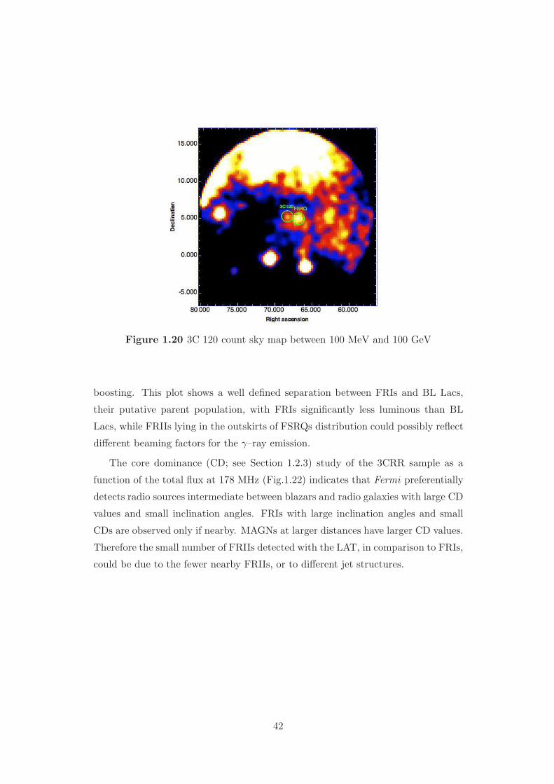
Figure 1.20 3C 120 count sky map between 100 MeV and 100 GeV
boosting. This plot shows a well defined separation between FRIs and BL Lacs,
their putative parent population, with FRIs significantly less luminous than BL
Lacs, while FRIIs lying in the outskirts of FSRQs distribution could possibly reflect
different beaming factors for the γ–ray emission.
The core dominance (CD; see Section 1.2.3) study of the 3CRR sample as a
function of the total flux at 178 MHz (Fig.1.22) indicates that Fermi preferentially
detects radio sources intermediate between blazars and radio galaxies with large CD
values and small inclination angles. FRIs with large inclination angles and small
CDs are observed only if nearby. MAGNs at larger distances have larger CD values.
Therefore the small number of FRIIs detected with the LAT, in comparison to FRIs,
could be due to the fewer nearby FRIIs, or to different jet structures.
42
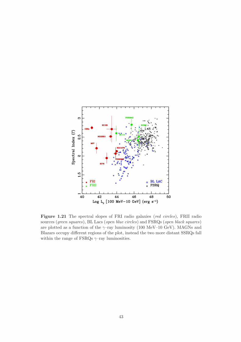
Figure 1.21 The spectral slopes of FRI radio galaxies (red circles), FRII radiosources (green squares), BL Lacs (open blue circles) and FSRQs (open black squares)are plotted as a function of the γ–ray luminosity (100 MeV–10 GeV). MAGNs andBlazars occupy different regions of the plot, instead the two more distant SSRQs fallwithin the range of FSRQs γ–ray luminosities.
43

Figure 1.22 Core dominance plotted against the total flux at 178 MHz of all thesources of the 3CRR sample: red circles represent FRIs and green squares FRIIs.The blue triangles in circles/squares are the MAGNs detected by Fermi and arecharacterized by large CD values. The blue triangles in empty black circles are thetwo FSRQs detected by LAT and have much larger CDs than MAGNs.
44
1.3.2 The jet structure of NGC 6251
The successive step, after having defined the MAGN sample, was to study in detail
one of the brightest radio galaxy in the sample: the FRI NGC 6251. In Migliori
et al. (2011) the study of the SED of the core is presented and the one zone syn-
chrotron/SSC framework is explored.
NGC 6251 is a luminous FRI, the fifth–brightest among the MAGNs, located at
z=0.0247. As other sources of the sample (Cen A, 3C 111, NGC 1275 and M87) it
was already detected by EGRET (Mukherjee et al. 2002). To construct the broad–
band nuclear SED, the radio to optical/UV data were collected from literature,
while for the high energy points, all available archival data, from XMM–Newton,
Swift and Chandra satellites, were re–analyzed. The XMM–Newton observation of
NGC 6251 (March 2002) was reduced using the SAS v.9.0 software and available
calibration files. Events affected by high flaring activity were discarded. The re-
sulting net exposure was 8.7 ks for the pn, 13.9 ks for the MOS1 and 13.5 ks for
the MOS2. The source and background spectra were extracted from circular re-
gions of 27′′ radius, and the response matrices created using the SAS commands
RMFGEN and ARFGEN. The nuclear data are not affected by pile–up. Data
were grouped to 25 counts per bin in order to apply the χ2 statistics. The best
fit (χ2/d.o.f.=410/372) for the pn spectrum (0.3–10 keV) consists of an absorbed
power law (NHGal=5.4×1020 cm−2; Kalberla et al. 2005) plus an APEC component
(kT∼0.6). There is no significant evidence for a Fe Kα emission line. These param-
eters are in agreement with those found by Evans et al. (2005). The same results
were obtained using the MOS data.
The Swift/X–Ray Telescope (XRT) observed NGC 6251 three times from April 2007
to May 2009. The X–ray data of the three observations were reduced using the on–
line XRT data analysis tool provided by the ASDC. 4 Source spectra were extracted
from a circular region of 20′′ radius, while background spectra were taken from an
annulus with an inner radius of 40′′ and outer radius of 80′′. Data were grouped to
20 counts per bin in order to apply the χ2 statistics. All spectral fits were performed
in the 0.5–10 keV band. The best–fit model is an absorbed power law with column
density slightly in excess of the Galactic value. The XRT spectra do not require the
addition of a soft thermal component, however notice that they are characterized
by low signal–to–noise ratio. Interestingly, during the XMM–Newton observation
the source appeared in a higher state (40% higher than Swift). A further change
4http://swift.asdc.asi.it/
45

in flux of about 15% was observed by Swift from 2007 to 2009 (see Fig. 1.23).
This ∼2 years represent the shortest period during which X–ray flux variability has
been detected, offering observational constraints on the nuclear origin of the γ–ray
emission. Instead, the fast (hour–scale) temporal variability is excluded from the
0.5–10 keV lightcurves of the four datasets.
Figure 1.23 Unfolded spectral model of the combined XMM–Newton and Swiftdatasets. Blue: XMM–Newton observation of March 2002; black: Swift observationof April 2007; red: Swift observation of May 2009; green: Swift observation of June2009.
The most recent (November 2003) and longest (49 ks) Chandra observation of
NGC 6251 was also analyzed. However the nuclear data were affected by pile–up,
estimated to be ≈13% using PIMMS 5, thus the Chandra nuclear fluxes were not
considered in the SED.
The nuclear SED from radio to gamma is dominated by non–thermal emis-
sion. It was modeled with both a single–zone SSC and a structured jet model
(Fig.1.24). When the SSC model is applied to the SED, it predicts lower Lorentz
factors (Γ ∼2.4) with respect to BL Lacs (Γ ∼10), implying that a simple extension
of BL Lac models to lower γ–ray luminosities FRI does not work. This poses serious
problems to the unified models. Indeed the jet structure can be different in FRIs,
as theorized by Ghisellini et al. (2005), with a fast inner component (the spine)
5http://cxc.harvard.edu/toolkit/pimms.jsp
46
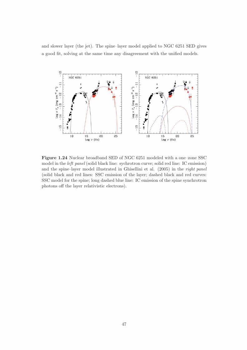
and slower layer (the jet). The spine–layer model applied to NGC 6251 SED gives
a good fit, solving at the same time any disagreement with the unified models.
Figure 1.24 Nuclear broadband SED of NGC 6251 modeled with a one–zone SSCmodel in the left panel (solid black line: sychrotron curve; solid red line: IC emission)and the spine–layer model illustrated in Ghisellini et al. (2005) in the right panel(solid black and red lines: SSC emission of the layer; dashed black and red curves:SSC model for the spine; long dashed blue line: IC emission of the spine synchrotronphotons off the layer relativistic electrons).
47

48

2High resolution X–ray
spectroscopy
X–ray astronomy was born between 1949, when X–ray radiation from the Sun was
revealed with detectors onboard sub–orbital rockets (Friedman et al. 1951), and
1962, when the very first extra–solar source, i.e. Scorpius X–1, was discovered by
Giacconi et al. (1962). During this half century life, huge steps forward were made in
improving the sensitivity of X–ray observatories. Until recently, detailed images and
spectra of cosmic sources were unavailable due to instrumental limitations. The first
X–ray satellites carried onboard gas proportional counters providing limited spectral
resolution (E/∆E∼ few). The Japan mission ASCA (Advanced Satellite for Cos-
mology and Astrophysics) launched in 1993, was the first observatory that, carrying
onboard Charge Coupled Devices (CCD) at the focus of the telescope, significantly
improved the spectral resolution (E/∆E≈10). The astrophysical world had to wait
Chandra and XMM–Newton satellites, NASA and ESA missions, respectively, both
launched in 1999 and still operating, to achieve an impressive spatial and spectral
resolution. A summary of what is the heritage of these two extraordinary missions
can be found in Santos–Lleo et al. (2010).
Chandra and XMM–Newton were the first observatories incorporating diffraction
grating spectrometers with E/∆E≥200 over the X–ray band 0.3–10 keV. Despite
being a relatively new research field, high–resolution X–ray spectroscopy provided
a wealth of information about cosmic X–ray sources, thanks to X–ray spectra with
unprecedented precision, allowing to study the physics of such objects.
The advent of high–resolution grating spectrometers made X–ray spectroscopy the
49
most powerful tool for investigating the ionized components of the gaseous AGN
environment. Indeed in many cases the gas temperature falls in the X–ray regime
because the virial temperature kT∼GMmp/R is in the range 106–108 K (e.g. ellipti-
cal galaxies, cluster of galaxies) or because of shocks heating the gas (e.g. supernova
remnants, binaries). The relative prominence of emission lines depends upon the
abundances of different elements, and the location of K–shell and L–shell transitions
associated with these elements within the X–ray band. The energies for the K– and
L–shell transitions can be roughly approximated (from Moseley’s formulae) as:
EK ∼ (10eV )Z2 (2.1)
and
EL ∼ (1.5eV )Z2 (2.2)
Thus the X–ray regime includes the K–shell features of Be (Z=4) through Ga
(Z=31) and the L–shell transitions of O (Z=16) through Tl (Z=81). However look-
ing at the standard cosmic abundances as represented in Fig. 2.1, it is evident
that abundances of elements like lithium, beryllium and boron are very low. In
addition, at high Z there is a very prominent abundance of iron (Z=26) that is a
consequence of nuclear stability. Infact 56Fe has the highest binding energy per
nucleus of any nucleus and acts as a divide between exothermic fusion reactions
(low Z) and endothermic ones. The X–ray band is therefore rich in discrete spectral
features, mainly due to: the K–shell (n=2→1) transitions of carbon though iron
and the L–shell (n=3→2) transitions of silicon through iron. Different charge states
are visible in an X–ray spectrum, unambiguously interpretable. Due to the high
radiative decay rate of X–ray transitions, astrophysical emitting plasmas are gen-
erally assumed not to be in local thermodynamic equilibrium (LTE), i.e. when the
particle distributions and level populations are in equilibrium but not the radiation
field. As a consequence, the derived spectra are sensitive to the physical conditions
in the source, in particular are strongly dependent on the mechanisms by which the
atomic levels are populated. In conclusion, investigating the single atomic features
in the X–ray spectrum means to make the physics of the plasma, measuring the
most important parameters without invoking any assumptions about the thermal
state of the gas.
50
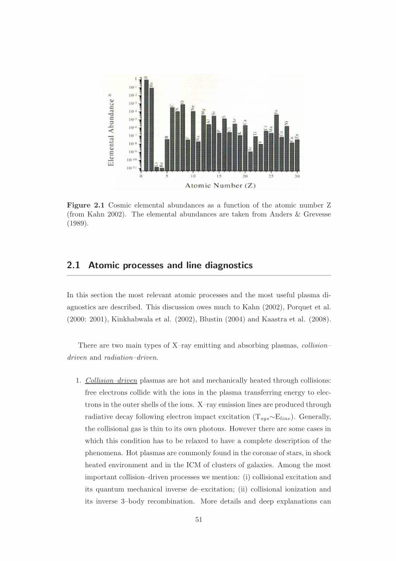
Figure 2.1 Cosmic elemental abundances as a function of the atomic number Z(from Kahn 2002). The elemental abundances are taken from Anders & Grevesse(1989).
2.1 Atomic processes and line diagnostics
In this section the most relevant atomic processes and the most useful plasma di-
agnostics are described. This discussion owes much to Kahn (2002), Porquet et al.
(2000: 2001), Kinkhabwala et al. (2002), Blustin (2004) and Kaastra et al. (2008).
There are two main types of X–ray emitting and absorbing plasmas, collision–
driven and radiation–driven.
1. Collision–driven plasmas are hot and mechanically heated through collisions:
free electrons collide with the ions in the plasma transferring energy to elec-
trons in the outer shells of the ions. X–ray emission lines are produced through
radiative decay following electron impact excitation (Tsys∼Eline). Generally,
the collisional gas is thin to its own photons. However there are some cases in
which this condition has to be relaxed to have a complete description of the
phenomena. Hot plasmas are commonly found in the coronae of stars, in shock
heated environment and in the ICM of clusters of galaxies. Among the most
important collision–driven processes we mention: (i) collisional excitation and
its quantum mechanical inverse de–excitation; (ii) collisional ionization and
its inverse 3–body recombination. More details and deep explanations can
51
be found in the following papers: Raymond & Smith (1977), Mewe et al.
(1985,1986), Kaastra (1992), Liedahl et al. (1995), Smith et al. (2001).
2. Radiation–driven photoionized plasmas are irradiated by a powerful external
source. X–ray emission lines are produced through recombination/radiative
cascade following photoionization, and radiative decay following photoexcita-
tion. The plasma temperature is lower with respect to collisional gas, consis-
tent with that necessary for photon heating. Photoionized plasmas have been
found in X–ray binaries, AGN outflows, cataclysmic variables, etc.
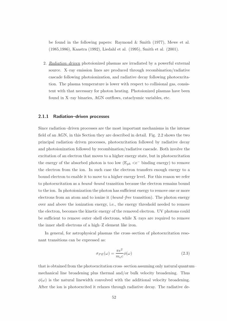
2.1.1 Radiation–driven processes
Since radiation–driven processes are the most important mechanisms in the intense
field of an AGN, in this Section they are described in detail. Fig. 2.2 shows the two
principal radiation–driven processes, photoexcitation followed by radiative decay
and photoionization followed by recombination/radiative cascade. Both involve the
excitation of an electron that moves to a higher energy state, but in photoexcitation
the energy of the absorbed photon is too low (Eph <e− binding energy) to remove
the electron from the ion. In such case the electron transfers enough energy to a
bound electron to enable it to move to a higher energy level. For this reason we refer
to photoexcitation as a bound–bound transition because the electron remains bound
to the ion. In photoionization the photon has sufficient energy to remove one or more
electrons from an atom and to ionize it (bound–free transition). The photon energy
over and above the ionization energy, i.e., the energy threshold needed to remove
the electron, becomes the kinetic energy of the removed electron. UV photons could
be sufficient to remove outer–shell electrons, while X–rays are required to remove
the inner shell electrons of a high–Z element like iron.
In general, for astrophysical plasmas the cross–section of photoexcitation reso-
nant transitions can be expressed as:
σPE(ω) =πe2
mecφ(ω) (2.3)
that is obtained from the photoexcitation cross–section assuming only natural quantum–
mechanical line broadening plus thermal and/or bulk velocity broadening. Thus
φ(ω) is the natural linewidth convolved with the additional velocity broadening.
After the ion is photoexcited it relaxes through radiative decay. The radiative de-
52
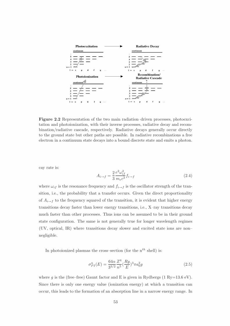
Figure 2.2 Representation of the two main radiation–driven processes, photoexci-tation and photoionization, with their inverse processes, radiative decay and recom-bination/radiative cascade, respectively. Radiative decays generally occur directlyto the ground state but other paths are possible. In radiative recombinations a freeelectron in a continuum state decays into a bound discrete state and emits a photon.
cay rate is:
Ai→f =2
3
e2ω2if
mec3fi→f (2.4)
where ωif is the resonance frequency and fi→f is the oscillator strength of the tran-
sition, i.e., the probability that a transfer occurs. Given the direct proportionality
of Ai→f to the frequency squared of the transition, it is evident that higher energy
transitions decay faster than lower energy transitions, i.e., X–ray transitions decay
much faster than other processes. Thus ions can be assumed to be in their ground
state configuration. The same is not generally true for longer wavelength regimes
(UV, optical, IR) where transitions decay slower and excited state ions are non–
negligible.
In photoionized plasmas the cross–section (for the nth shell) is:
σnPI(E) =
64α
33/2
Z4
n5(Ry
E)3πa2
0g (2.5)
where g is the (free–free) Gaunt factor and E is given in Rydbergs (1 Ry=13.6 eV).
Since there is only one energy value (ionization energy) at which a transition can
occur, this leads to the formation of an absorption line in a narrow energy range. In
53

case of photoionization when a bound–free transition takes place, the electron can
be removed by any photon with an energy greater than the threshold. Consequently,
the absorption feature produced by a bound–free transition is very spread–out: it is
deepest at the ionization energy and becomes weaker with increasing energy (Blustin
2004).
The inverse process to photoionization is radiative recombination. A free electron
in a continuum state decays into a bound discrete state through the emission of a
photon:
e− + ion → photon (2.6)
If the distribution is thermal (Maxwellian), the shape of the resulting radiative re-
combination continua (RRC) is determined by the electron temperature Te. From
the width of RRC features, it is possible to derive a direct measurement of the
recombining electron temperature (Liedahl & Paerels 1996) as shown in Fig. 2.3.
In a collisional plasma electrons have high temperatures, so the RRC will be broad
and shallow, difficult to distinguish from the underlying thermal continuum. On
the other hand, when the plasma is photoionized, the electrons are at a lower tem-
perature for the same level of ionization with a narrower distribution of energies.
Thus the RRC are narrow and prominent features at the ionization energy (i.e.
absorption edge position) of a given ion.
Other two radiation–driven processes have to be mentioned: the fluorescence
and the autoionization. The fluorescence process involvs two steps. In the first step
a photon with an energy above the K–shell photoionization threshold energy ionizes
a 1s electron. In the second step the excited state can decay through the emission
of a photon (fluorescence). In the radiative decay a bound electron fills the 1s hole
leaving a vacancy in another shell.The most probable radiative decay involves a n=2
→ n=1 transition (Kα) . It is appreciable for high Z–elements since the radiative
decay scales like Z4 (see Section 2.1.2 for details).
More often states with holes in the K–shell will autoionize (autoionization) eject-
ing a second electron (the Auger effect), leaving the atom in the next highest stage
of ionization. If the atom is not stabilized it can undergo further Auger decays.
This process dominates for low–Z elements. Autoionization of an atom can also
occur without the capture of radiation. It occurs when an ion captures a free
electron, that expends the lost energy in exciting a core electron. The resulting
atom is doubly excited. It can decay by autoionization ejecting the electron into
the continuum (in this case there is no change of charge in the level of ionization
54
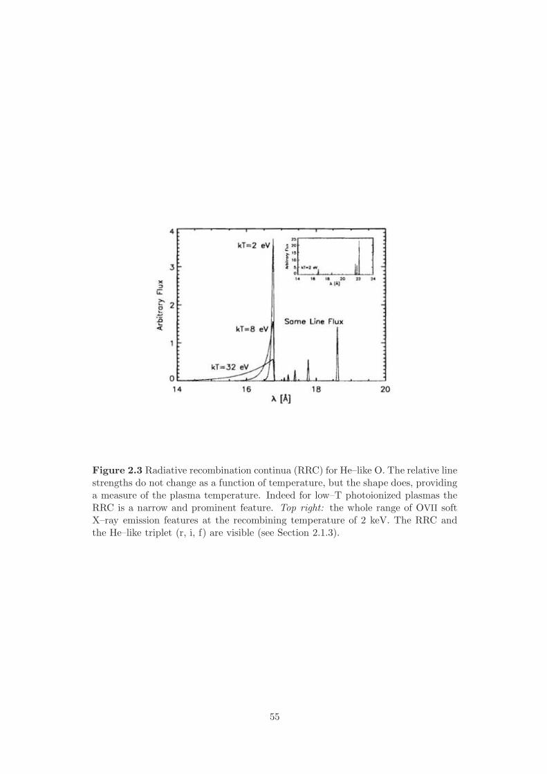
Figure 2.3 Radiative recombination continua (RRC) for He–like O. The relative linestrengths do not change as a function of temperature, but the shape does, providinga measure of the plasma temperature. Indeed for low–T photoionized plasmas theRRC is a narrow and prominent feature. Top right: the whole range of OVII softX–ray emission features at the recombining temperature of 2 keV. The RRC andthe He–like triplet (r, i, f) are visible (see Section 2.1.3).
55
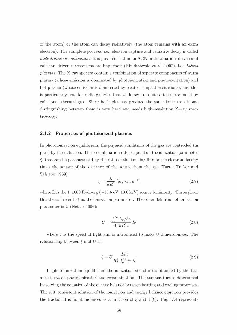
of the atom) or the atom can decay radiatively (the atom remains with an extra
electron). The complete process, i.e., electron capture and radiative decay is called
dielectronic recombination. It is possible that in an AGN both radiation–driven and
collision–driven mechanisms are important (Kinkhabwala et al. 2002), i.e., hybrid
plasmas. The X–ray spectra contain a combination of separate components of warm
plasma (whose emission is dominated by photoionization and photoexcitation) and
hot plasma (whose emission is dominated by electron impact excitations), and this
is particularly true for radio galaxies that we know are quite often surrounded by
collisional thermal gas. Since both plasmas produce the same ionic transitions,
distinguishing between them is very hard and needs high–resolution X–ray spec-
troscopy.
2.1.2 Properties of photoionized plasmas
In photoionization equilibrium, the physical conditions of the gas are controlled (in
part) by the radiation. The recombination rates depend on the ionization parameter
ξ, that can be parametrized by the ratio of the ionizing flux to the electron density
times the square of the distance of the source from the gas (Tarter Tucker and
Salpeter 1969):
ξ =L
nR2[erg cm s−1] (2.7)
where L is the 1–1000 Rydberg (∼13.6 eV–13.6 keV) source luminosity. Throughout
this thesis I refer to ξ as the ionization parameter. The other definition of ionization
parameter is U (Netzer 1996):
U =
∫ ∞
νLν/hν
4πnR2cdν (2.8)
where c is the speed of light and is introduced to make U dimensionless. The
relationship between ξ and U is:
ξ = ULhc
R2L
∫ ∞
νfν
ν dν(2.9)
In photoionization equilibrium the ionization structure is obtained by the bal-
ance between photoionization and recombination. The temperature is determined
by solving the equation of the energy balance between heating and cooling processes.
The self–consistent solution of the ionization and energy balance equation provides
the fractional ionic abundances as a function of ξ and T(ξ). Fig. 2.4 represents
56
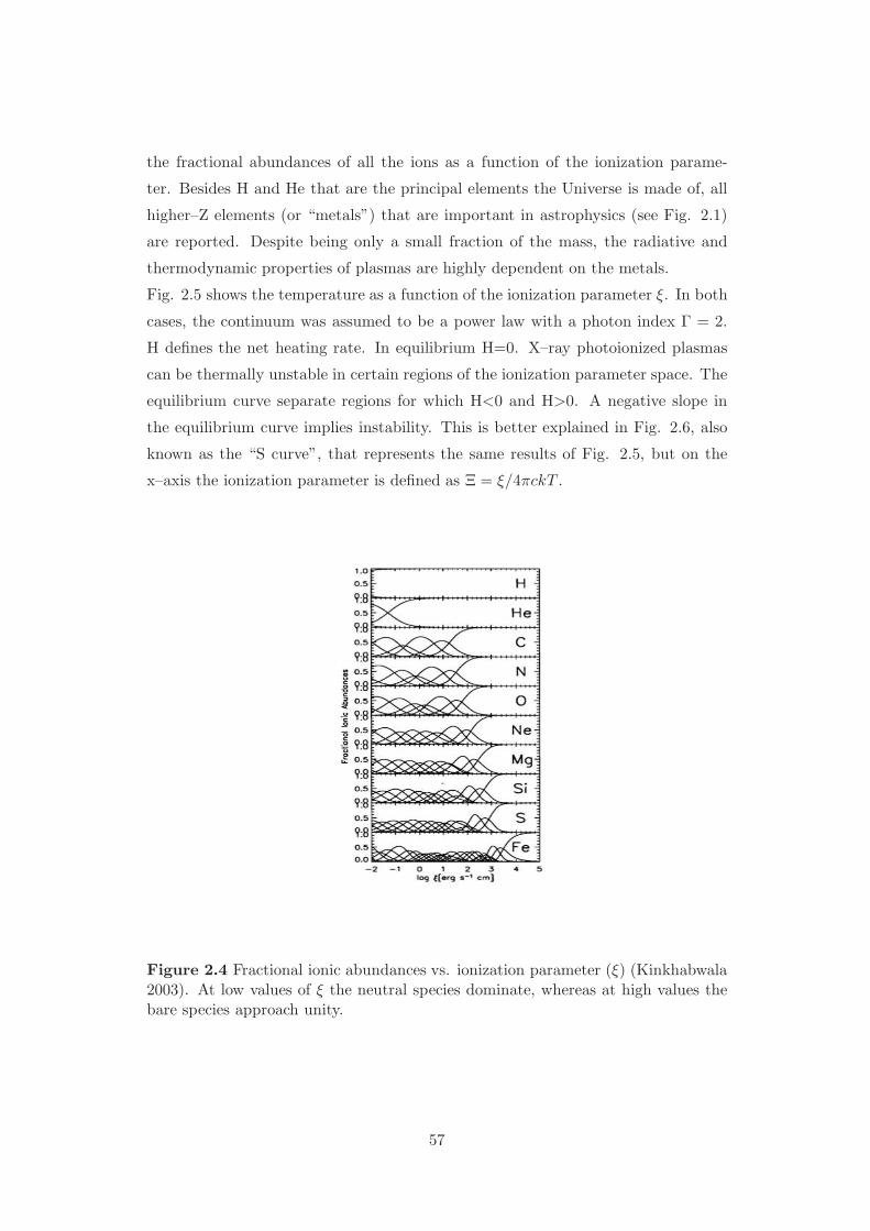
the fractional abundances of all the ions as a function of the ionization parame-
ter. Besides H and He that are the principal elements the Universe is made of, all
higher–Z elements (or “metals”) that are important in astrophysics (see Fig. 2.1)
are reported. Despite being only a small fraction of the mass, the radiative and
thermodynamic properties of plasmas are highly dependent on the metals.
Fig. 2.5 shows the temperature as a function of the ionization parameter ξ. In both
cases, the continuum was assumed to be a power law with a photon index Γ = 2.
H defines the net heating rate. In equilibrium H=0. X–ray photoionized plasmas
can be thermally unstable in certain regions of the ionization parameter space. The
equilibrium curve separate regions for which H<0 and H>0. A negative slope in
the equilibrium curve implies instability. This is better explained in Fig. 2.6, also
known as the “S curve”, that represents the same results of Fig. 2.5, but on the
x–axis the ionization parameter is defined as Ξ = ξ/4πckT .
Figure 2.4 Fractional ionic abundances vs. ionization parameter (ξ) (Kinkhabwala2003). At low values of ξ the neutral species dominate, whereas at high values thebare species approach unity.
57
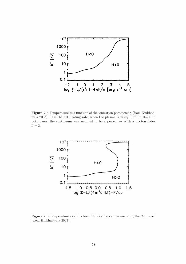
Figure 2.5 Temperature as a function of the ionization parameter ξ (from Kinkhab-wala 2003). H is the net heating rate, when the plasma is in equilibrium H=0. Inboth cases, the continuum was assumed to be a power law with a photon indexΓ = 2.
Figure 2.6 Temperature as a function of the ionization parameter Ξ, the “S–curve”(from Kinkhabwala 2003).
58
2.1.3 Plasma diagnostics
The spectral features formed are sensitive to the physical conditions in the gas.
Thus they can be used as density and temperature diagnostics to discriminate be-
tween collisional or photoionized gas. However, as it is described below, not all the
transitions have the same diagnostic utility.
The most prominent emission lines in the spectrum of X–ray emitting plasmas are:
1. the Lyman series transitions of H–like ions;
2. the He–like K–shell transitions;
3. the Fe L–shell transitions.
1) The Lyman series transitions (n≥2→n=1) are typical of low–Z abundant el-
ements found in their H–like charge state (one electron left). These are degenerate
transitions depending on the fine structure of the level:
Lyα1: 1s–2p 2P3/2; Lyα2: 1s–2p 2P1/2
Lyβ1: 1s–3p 2P3/2; Lyβ2: 1s–3p 2P1/2
Lyγ1: 1s–4p 2P3/2; Lyγ2: 1s–4p 2P1/2
all produced through electric dipole transitions. Despite their prominence, the
diagnostic utility of Lyman series transitions is limited. The line ratios are only
slightly different for collisional and photoionized plasmas, making challenging a
solid conclusion on the driving mechanism (Fig. 2.7).
2) The He–like (two electrons left) K–shell transitions are of great importance in
the soft X–ray band. These are triplets of emission lines whose ratios are sensitive
to the density, temperature and ionization mechanism of the plasma. Being He–like
charge state a very tight closed shell this is the dominant ion species over a wide
range in temperature. The most important He-like transitions, also called He–like
triplets, are:
R(or W): 1s2 1S0–1s2p 1P1 resonance line
I(or X+Y): 1s2 1S0–1s2p 3P2; 1s2 1S0–1s2p 3P1 intercombination line
F(or Z): 1s2 1S0–1s2p 3S1 forbidden line
The resonance line is an allowed electric dipole transition, while the forbidden
line is a relativistic magnetic dipole transition characterized by a very low radiative
59
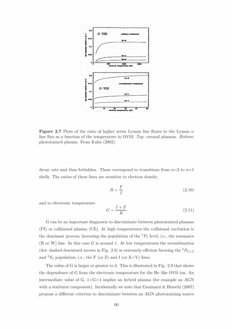
Figure 2.7 Plots of the ratio of higher series Lyman line fluxes to the Lyman αline flux as a function of the temperature in OVIII. Top: coronal plasmas. Bottom:photoionized plasma. From Kahn (2002).
decay rate and thus forbidden. These correspond to transitions from n=2 to n=1
shells. The ratios of these lines are sensitive to electron density
R =F
I(2.10)
and to electronic temperature
G =I + F
R(2.11)
G can be an important diagnostic to discriminate between photoionized plasmas
(PI) or collisional plasma (CE). At high temperatures the collisional excitation is
the dominant process, favouring the population of the 1P1 level, i.e., the resonance
(R or W) line. In this case G is around 1. At low temperatures the recombination
(dot–dashed downward arrows in Fig. 2.8) is extremely efficient favoring the 3P0,1,2
and 3S1 population, i.e., the F (or Z) and I (or X+Y) lines.
The value of G is larger or greater to 4. This is illustrated in Fig. 2.9 that shows
the dependence of G from the electronic temperature for the He–like OVII ion. An
intermediate value of G, 1<G<4 implies an hybrid plasma (for example an AGN
with a starburst component). Incidentally we note that Guainazzi & Bianchi (2007)
propose a different criterion to discriminate between an AGN photoionizing source
60
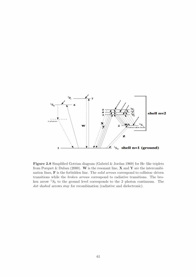
Figure 2.8 Simplified Gotrian diagram (Gabriel & Jordan 1969) for He–like tripletsfrom Porquet & Dubau (2000). W is the resonant line, X and Y are the intercombi-nation lines, F is the forbidden line. The solid arrows correspond to collision–driventransitions while the broken arrows correspond to radiative transitions. The bro-ken arrow 1S0 to the ground level corresponds to the 2–photon continuum. Thedot–dashed arrows stay for recombination (radiative and dielectronic).
61
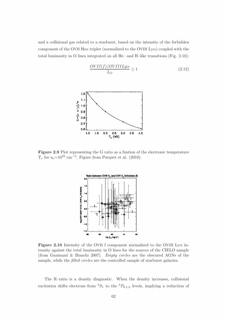
and a collisional gas related to a starburst, based on the intensity of the forbidden
component of the OVII Heα triplet (normalized to the OVIII Lyα) coupled with the
total luminosity in O lines integrated on all He– and H–like transitions (Fig. 2.10):
OV II(f)/OV IIILyα
LO≥ 1 (2.12)
Figure 2.9 Plot representing the G ratio as a funtion of the electronic temperatureTe for ne=1010 cm−3. Figure from Porquet et al. (2010).
Figure 2.10 Intensity of the OVII f component normalized to the OVIII Lyα in-tensity against the total luminosity in O lines for the sources of the CIELO sample(from Guainazzi & Bianchi 2007). Empty circles are the obscured AGNs of thesample, while the filled circles are the controlled sample of starburst galaxies.
The R–ratio is a density diagnostic. When the density increases, collisional
excitation shifts electrons from 3S1 to the 3P0,1,2 levels, implying a reduction of
62
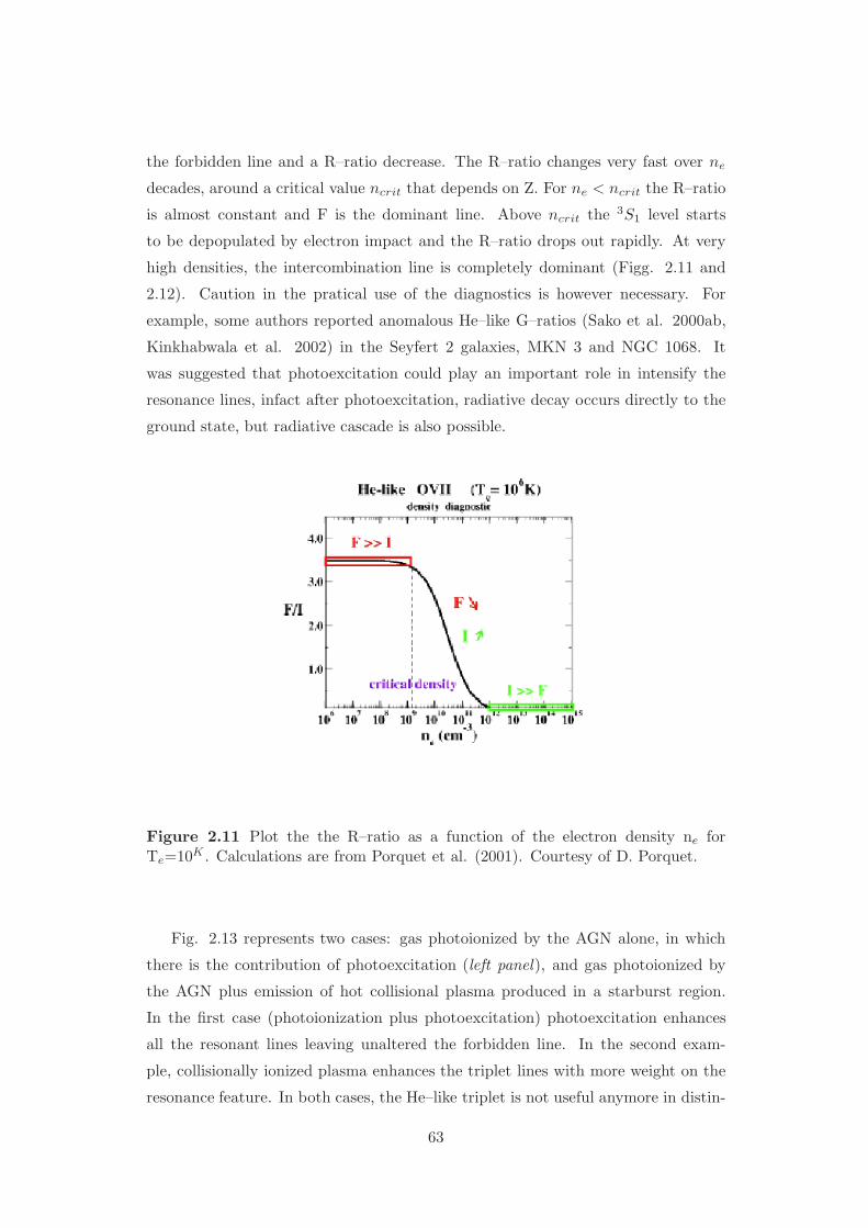
the forbidden line and a R–ratio decrease. The R–ratio changes very fast over ne
decades, around a critical value ncrit that depends on Z. For ne < ncrit the R–ratio
is almost constant and F is the dominant line. Above ncrit the 3S1 level starts
to be depopulated by electron impact and the R–ratio drops out rapidly. At very
high densities, the intercombination line is completely dominant (Figg. 2.11 and
2.12). Caution in the pratical use of the diagnostics is however necessary. For
example, some authors reported anomalous He–like G–ratios (Sako et al. 2000ab,
Kinkhabwala et al. 2002) in the Seyfert 2 galaxies, MKN 3 and NGC 1068. It
was suggested that photoexcitation could play an important role in intensify the
resonance lines, infact after photoexcitation, radiative decay occurs directly to the
ground state, but radiative cascade is also possible.
Figure 2.11 Plot the the R–ratio as a function of the electron density ne forTe=10K . Calculations are from Porquet et al. (2001). Courtesy of D. Porquet.
Fig. 2.13 represents two cases: gas photoionized by the AGN alone, in which
there is the contribution of photoexcitation (left panel), and gas photoionized by
the AGN plus emission of hot collisional plasma produced in a starburst region.
In the first case (photoionization plus photoexcitation) photoexcitation enhances
all the resonant lines leaving unaltered the forbidden line. In the second exam-
ple, collisionally ionized plasma enhances the triplet lines with more weight on the
resonance feature. In both cases, the He–like triplet is not useful anymore in distin-
63
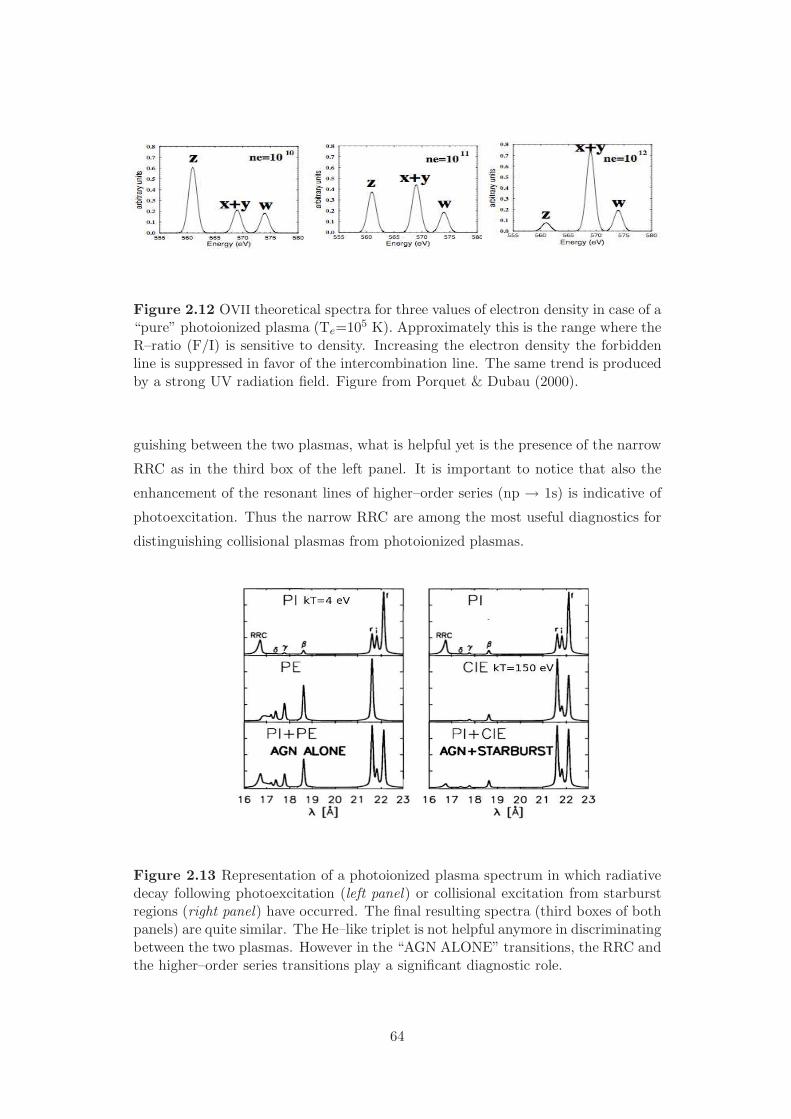
Figure 2.12 OVII theoretical spectra for three values of electron density in case of a“pure” photoionized plasma (Te=105 K). Approximately this is the range where theR–ratio (F/I) is sensitive to density. Increasing the electron density the forbiddenline is suppressed in favor of the intercombination line. The same trend is producedby a strong UV radiation field. Figure from Porquet & Dubau (2000).
guishing between the two plasmas, what is helpful yet is the presence of the narrow
RRC as in the third box of the left panel. It is important to notice that also the
enhancement of the resonant lines of higher–order series (np → 1s) is indicative of
photoexcitation. Thus the narrow RRC are among the most useful diagnostics for
distinguishing collisional plasmas from photoionized plasmas.
Figure 2.13 Representation of a photoionized plasma spectrum in which radiativedecay following photoexcitation (left panel) or collisional excitation from starburstregions (right panel) have occurred. The final resulting spectra (third boxes of bothpanels) are quite similar. The He–like triplet is not helpful anymore in discriminatingbetween the two plasmas. However in the “AGN ALONE” transitions, the RRC andthe higher–order series transitions play a significant diagnostic role.
64
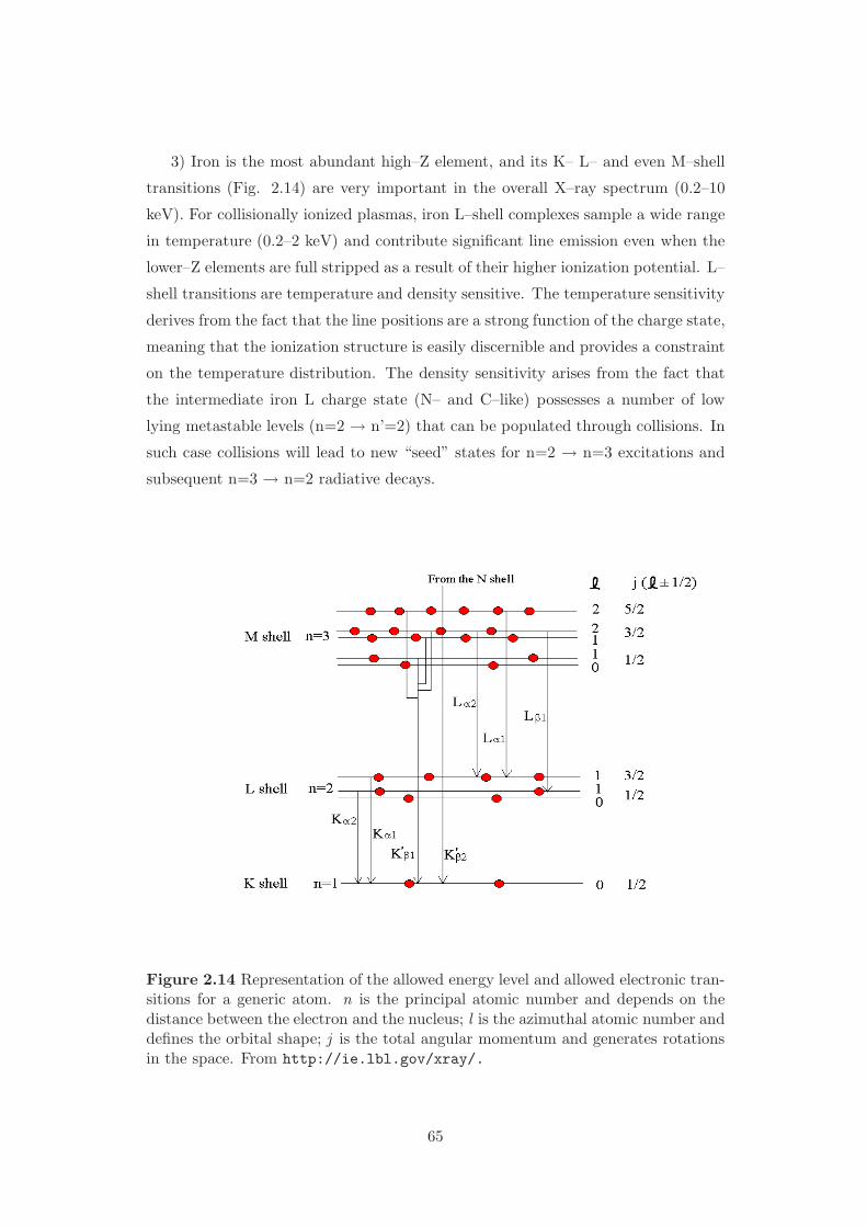
3) Iron is the most abundant high–Z element, and its K– L– and even M–shell
transitions (Fig. 2.14) are very important in the overall X–ray spectrum (0.2–10
keV). For collisionally ionized plasmas, iron L–shell complexes sample a wide range
in temperature (0.2–2 keV) and contribute significant line emission even when the
lower–Z elements are full stripped as a result of their higher ionization potential. L–
shell transitions are temperature and density sensitive. The temperature sensitivity
derives from the fact that the line positions are a strong function of the charge state,
meaning that the ionization structure is easily discernible and provides a constraint
on the temperature distribution. The density sensitivity arises from the fact that
the intermediate iron L charge state (N– and C–like) possesses a number of low
lying metastable levels (n=2 → n’=2) that can be populated through collisions. In
such case collisions will lead to new “seed” states for n=2 → n=3 excitations and
subsequent n=3 → n=2 radiative decays.
Figure 2.14 Representation of the allowed energy level and allowed electronic tran-sitions for a generic atom. n is the principal atomic number and depends on thedistance between the electron and the nucleus; l is the azimuthal atomic number anddefines the orbital shape; j is the total angular momentum and generates rotationsin the space. From http://ie.lbl.gov/xray/.
65
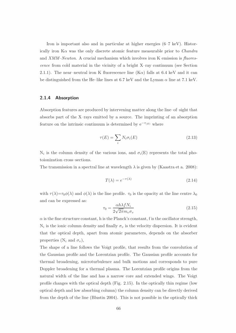
Iron is important also and in particular at higher energies (6–7 keV). Histor-
ically iron Kα was the only discrete atomic feature measurable prior to Chandra
and XMM–Newton. A crucial mechanism which involves iron K emission is fluores-
cence from cold material in the vicinity of a bright X–ray continuum (see Section
2.1.1). The near–neutral iron K fluorescence line (Kα) falls at 6.4 keV and it can
be distinguished from the He–like lines at 6.7 keV and the Lyman α line at 7.1 keV.
2.1.4 Absorption
Absorption features are produced by intervening matter along the line–of–sight that
absorbs part of the X–rays emitted by a source. The imprinting of an absorption
feature on the intrinsic continuum is determined by e−τ(E) where
τ(E) =∑
i
Niσi(E) (2.13)
Ni is the column density of the various ions, and σi(E) represents the total pho-
toionization cross–sections.
The transmission in a spectral line at wavelength λ is given by (Kaastra et a. 2008):
T (λ) = e−τ(λ) (2.14)
with τ(λ)=τ0φ(λ) and φ(λ) is the line profile. τ0 is the opacity at the line centre λ0
and can be expressed as:
τ0 =αhλfNi
2√
2πmeσv
(2.15)
α is the fine structure constant, h is the Planck’s constant, f is the oscillator strength,
Ni is the ionic column density and finally σv is the velocity dispersion. It is evident
that the optical depth, apart from atomic parameters, depends on the absorber
properties (Ni and σv),
The shape of a line follows the Voigt profile, that results from the convolution of
the Gaussian profile and the Lorentzian profile. The Gaussian profile accounts for
thermal broadening, microturbulence and bulk motions and corresponds to pure
Doppler broadening for a thermal plasma. The Lorentzian profile origins from the
natural width of the line and has a narrow core and extended wings. The Voigt
profile changes with the optical depth (Fig. 2.15). In the optically thin regime (low
optical depth and low absorbing column) the column density can be directly derived
from the depth of the line (Blustin 2004). This is not possible in the optically thick
66
regime because the line is saturated, and absorbs away all the continuum flux at its
central wavelength.
Figure 2.15 Voigt profile plotted at a range of optical depth (from Blustin 2004).x’=λ-λ0.
The strength (or depth) of a line is measured by the equivalent width (EW) and
is the area of the spectral continuum taken up by the line. It is calculated from:
EW =
∫(Fc − Fλ)
Fcdλ (2.16)
Fλ is the flux in the interested area of the line, Fc is the flux of the continuum.
Absorption lines can be of several types. There are the strong resonance lines
involving the outermost atomic shells like the OVII 1s–2p at 21.6 A and OVIII Lyα
doublet at 18.97 A , or the inner–shell absorption lines. The absorption lines could
be well resolved or strongly blended because neither they are produced by higher
principal quantum number transitions nor the column density is very high (Kaastra
et al. 2008). The iron M–shell (n=2 → 3) transitions of FeI – FeXVI are an example
of strongly blended lines. They manifest themselves as a broad absorption feature
around 16–17 A . This feature is hard to resolve spectroscopically and has been
identified as unresolved transition array (UTA) mainly due to 2p–3d inner shell
absorption in M–shell iron (Sako et al. 2001; Behar et al. 2001; Netzer et al. 2004).
Before the advent of high–resolution grating spectrometers this structure might be
identified as an OVII edge. The equivalent width (EW) and central wavelength of
the UTA are potentially important diagnostics of AGN absorbers. An example of
67
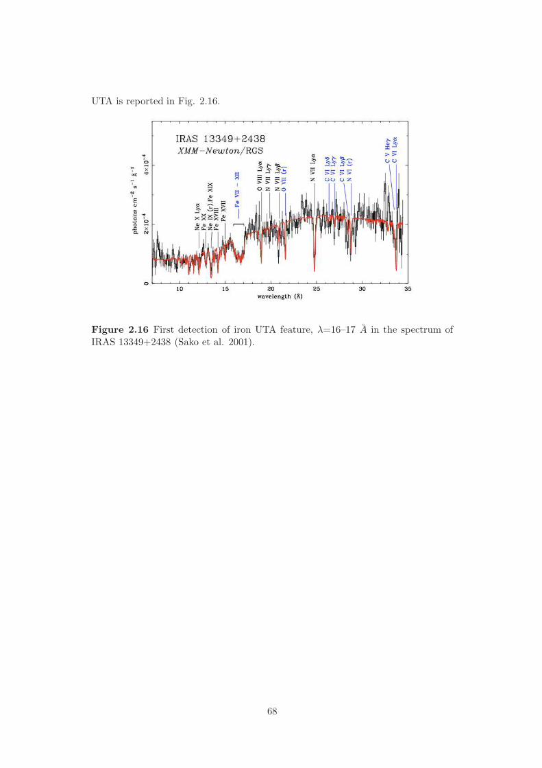
UTA is reported in Fig. 2.16.
Figure 2.16 First detection of iron UTA feature, λ=16–17 A in the spectrum ofIRAS 13349+2438 (Sako et al. 2001).
68

3Warm photoionized gas in emission
The spectrum observed from a photoionized medium depends on the relative orien-
tation of the irradiating source, the irradiated medium and the observer. Fig. 3.1
represents a sketch of the two extreme cases of orientation: in the “Absorption”
direction the relative soft X–ray spectrum will result in discrete line absorption
(photoexcitation) plus photoelectric edge absorption (photoionization) correspond-
ing to the upper panel of Fig. 3.2. This is a typical Seyfert 1 spectrum in which the
central engine is not obscured by an intervening medium, i.e. the torus, and the
features produced by the warm absorber (see Chapter 4) are detected.
If the orientation is in the “Reemission” direction, the X–ray intrinsic contin-
uum is blocked by a dusty torus allowing only reprocessed radiation to be visible
in the spectrum (Fig. 3.2 bottom panel). In this scenario all photoexcitations and
photoionizations are balanced by radiative decays and recombination/radiative cas-
cades. Seyfert 2s are characterized by similar spectra.
The detection and identification of emission lines in Seyfert 2 galaxies, thanks
to high–resolution X–ray spectroscopy, has revealed large scale emitting gas (kT ∼few keV), photoionized by the nuclear engine (Sako et al. 2000; Kinkhabwala et al.
2002; Bianchi et al. 2005; Pounds & Vaughan 2006; Guainazzi & Bianchi 2007).
Spatially resolved studies performed with the Chandra telescope for at least the
three brightest AGNs, NGC 1068 (Kinkhabwala et al. 2002; Brinkman et al. 2002;
Ogle et al. 2003), Circinus (Sambruna et al. 2001), and Mrk 3 (Sako et al. 2000ab;
Bianchi et al. 2005; Pounds & Page 2005), have pointed out that the soft X-ray
emission originates in regions extended on hundreds of pc, and its dimension and
morphology closely resembles that of the Narrow Line Region (NLR) as mapped by
69
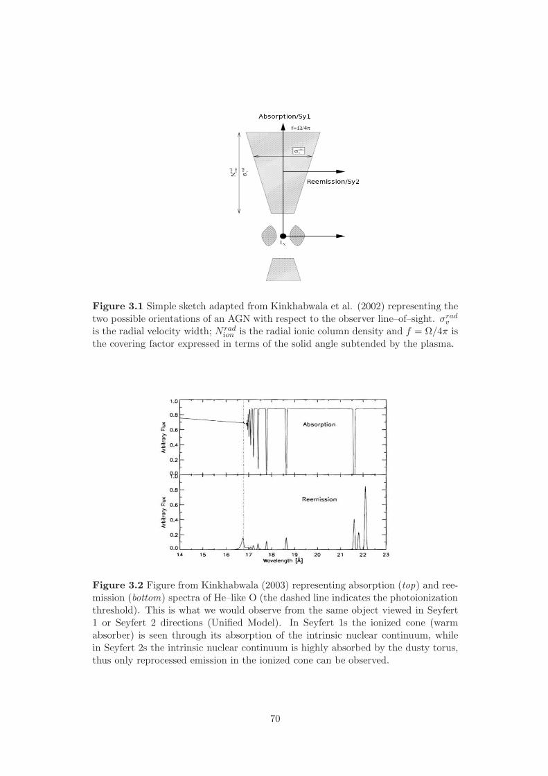
Figure 3.1 Simple sketch adapted from Kinkhabwala et al. (2002) representing thetwo possible orientations of an AGN with respect to the observer line–of–sight. σrad
v
is the radial velocity width; N radion is the radial ionic column density and f = Ω/4π is
the covering factor expressed in terms of the solid angle subtended by the plasma.
Figure 3.2 Figure from Kinkhabwala (2003) representing absorption (top) and ree-mission (bottom) spectra of He–like O (the dashed line indicates the photoionizationthreshold). This is what we would observe from the same object viewed in Seyfert1 or Seyfert 2 directions (Unified Model). In Seyfert 1s the ionized cone (warmabsorber) is seen through its absorption of the intrinsic nuclear continuum, whilein Seyfert 2s the intrinsic nuclear continuum is highly absorbed by the dusty torus,thus only reprocessed emission in the ionized cone can be observed.
70

the optical [OIII]λ5007 emission line (e.g. Bianchi, Guainazzi & Chiaberge 2006).
Concerning Radio–Loud AGNs, the attention has been addressed so far to the ex-
traordinary phenomena related to the jets at kpc scales. The relativistic plasma
produces bright hot spots interacting with the environment, excavates cavities in
the intracluster medium (ICM) and upscatters microwave background photons. Nu-
clear and circumnuclear environment has not yet been studied with the same effort.
This is not surprising since RL AGNs are intrinsically complex sources, because
the relativistic jet blurres the overall picture making hard to disentangle its non-
thermal emission from other kinds of radiation. For example, the X–ray spectrum
of FRII radio galaxies optically classified as High Excitation Galaxies (HEG) are
quite similar to Seyfert 2s. They show a heavily obscured emission (intrinsic column
density ∼ 1023−24 cm−2) and a soft unabsorbed tail (Belsole et al. 2006; Hardcastle
et al. 2006; Evans et al. 2006). While the former component is clearly related to
the bright accretion disk obscured by an edge–on oriented thick torus, the nature
of the soft excess was not immediately understood. At first it was proposed that
soft photons originate from the jet emerging from the top of the torus. However the
discovery of photoionized emission lines in the soft X–ray spectrum of the obscured
BLRG 3C 445 (Grandi et al. 2007; Sambruna et al. 2007; Reeves et al. 2010) and
in the type 2 quasar 3C 234 (Piconcelli et al. 2008) weakened this hypothesis and
opened a new and alternative way to interpret the soft excess.
The study of the NLRG 3C 33 (Torresi et al. 2009), that is part of this thesis, is
a work in strong support to the thermal interpretation of the soft excess in radio
galaxies.
3.1 Evidence of photoionized gas in the soft X–ray spectrum
of 3C 33
This section describes the X-ray data analysis of the NLRG 3C 33. All the ob-
servations available in the Chandra and XMM-Newton archives have been used to
investigate the X-ray spectral properties of this source. The main result is the de-
tection in both ACIS and EPIC spectra of emission lines in the 0.5–2 keV band, that
can be attributed to photoionized emitting gas. Unfortunately, due to the shortness
of the XMM–Newton observation, and consequently to the low S/N ratio, the RGS
data could not be used.
71
3.1.1 Introduction
3C 33 is the ideal target to investigate the nature of the soft excess. It is a genuine
type II radio galaxy (L178=7.5×1025 W Hz−1 sr−1), optically classified as High
Excitation Galaxy (HEG) and one of closest HEG in the 3CRR catalogue (Laing,
Riley & Longair 1983) located at z=0.0597 (Popescu et al. 1996).
It exhibits symmetric lobes with hot spots on kpc scale (Leahy & Perley 1991), and
two symmetric jets in the VLBI image (Giovannini et al. 2005). The southern jet
is stronger by a factor 2 at 5 mas. Expressing the jet/counterjet ratio (J) in terms
of the bulk velocity of the jet (β) and the angle between the jet and the line–of–
sight (θ) (see Section 1.2.3), an inclination angle of 75 − 80 can be deduced. Its
spatial orientation is then favorable for revealing soft X–ray emission lines, because
a strong de–amplification of the jet radiation is expected. Fig. 3.3 represents the
unsmoothed Chandra 0.3–2 keV image with 1.5 GHz radio conoturs overlaid.
Moreover 3C 33 is very luminous in the [OIII] band (L[OIII] ∼1.09×1042 erg s−1)
exhibiting the highest [OIII] flux of all nearby NLRGs (z<0.3) in the 3CRR sample.
This is a very important observational property since the [OIII]λ5007 emission line
is a powerful tracer of the NLR.
Previous nuclear observations of 3C 33 in the X–ray band date to those of the
EINSTEIN (Fabbiano et al. 1984) and ROSAT (Hardcastle et al. 1998; Hardcastle
et al. 1999) X–ray telescopes. EINSTEIN only provided an upper limit to the 0.5–3
keV luminosity, while ROSAT/HRI could detect the source in the soft X–ray band,
although the HRI instrument onboard was not able to resolve the source.
Evans et al. (2006) analyzed the XMM-Newton EPIC pn data of 3C 33 showing for
the first time the Seyfert 2 nature of its hard component. They modeled the soft
component with an unabsorbed power law.
Taking advantage of the unprecedented imaging of Chandra, Kraft et al. (2007)
performed a detailed spatial study of 3C 33, resolving the north and south hot–spot
regions. They also studied the nuclear component with a basic model consisting of
an absorbed power law plus a Fe Kα line. The soft part was fitted with a collisional
gas model associated to the clearly extended structure around the unresolved hard
nucleus. A similar elongation was observed in the Hubble Space Telescope WFPC1
and WFPC2 imaging, and was interpreted by the authors as a tracer of stellar dis-
tribution.
Large residuals between 1 and 3 keV, still present in the Chandra spectrum, were ex-
plained by assuming the presence of either a reflection component or a less absorbed
72
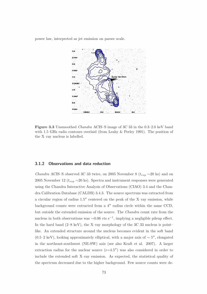
power law, interpreted as jet emission on parsec scale.
Figure 3.3 Unsmoothed Chandra ACIS–S image of 3C 33 in the 0.3–2.0 keV bandwith 1.5 GHz radio contours overlaid (from Leahy & Perley 1991). The position ofthe X–ray nucleus is labelled.
3.1.2 Observations and data reduction
Chandra ACIS–S observed 3C 33 twice, on 2005 November 8 (texp ∼20 ks) and on
2005 November 12 (texp ∼20 ks). Spectra and instrument responses were generated
using the Chandra Interactive Analysis of Observations (CIAO) 3.4 and the Chan-
dra Calibration Database (CALDB) 3.4.3. The source spectrum was extracted from
a circular region of radius 1.5′′ centered on the peak of the X–ray emission, while
background counts were extracted from a 4′′ radius circle within the same CCD,
but outside the extended emission of the source. The Chandra count rate from the
nucleus in both observations was ∼0.06 cts s−1, implying a negligible pileup effect.
In the hard band (2–8 keV), the X–ray morphology of the 3C 33 nucleus is point–
like. An extended structure around the nucleus becomes evident in the soft band
(0.5–2 keV), looking approximately elliptical, with a major axis of ∼ 5′′, elongated
in the northeast-southwest (NE-SW) axis (see also Kraft et al. 2007). A larger
extraction radius for the nuclear source (r=4.5′′) was also considered in order to
include the extended soft X–ray emission. As expected, the statistical quality of
the spectrum decreased due to the higher background. Few source counts were de-
73
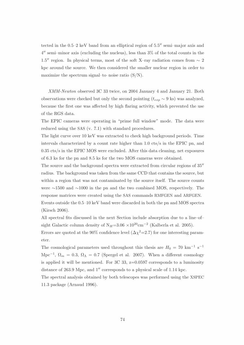
tected in the 0.5–2 keV band from an elliptical region of 5.5′′ semi–major axis and
4′′ semi–minor axis (excluding the nucleus), less than 3% of the total counts in the
1.5′′ region. In physical terms, most of the soft X–ray radiation comes from ∼ 2
kpc around the source. We then considered the smaller nuclear region in order to
maximize the spectrum signal–to–noise ratio (S/N).
XMM-Newton observed 3C 33 twice, on 2004 January 4 and January 21. Both
observations were checked but only the second pointing (texp ∼ 9 ks) was analyzed,
because the first one was affected by high flaring activity, which prevented the use
of the RGS data.
The EPIC cameras were operating in “prime full window” mode. The data were
reduced using the SAS (v. 7.1) with standard procedures.
The light curve over 10 keV was extracted to check high background periods. Time
intervals characterized by a count rate higher than 1.0 cts/s in the EPIC pn, and
0.35 cts/s in the EPIC MOS were excluded. After this data cleaning, net exposures
of 6.3 ks for the pn and 8.5 ks for the two MOS cameras were obtained.
The source and the background spectra were extracted from circular regions of 35′′
radius. The background was taken from the same CCD that contains the source, but
within a region that was not contaminated by the source itself. The source counts
were ∼1500 and ∼1000 in the pn and the two combined MOS, respectively. The
response matrices were created using the SAS commands RMFGEN and ARFGEN.
Events outside the 0.5–10 keV band were discarded in both the pn and MOS spectra
(Kirsch 2006).
All spectral fits discussed in the next Section include absorption due to a line–of–
sight Galactic column density of NH=3.06 ×1020cm−2 (Kalberla et al. 2005).
Errors are quoted at the 90% confidence level (∆χ2=2.7) for one interesting param-
eter.
The cosmological parameters used throughout this thesis are H0 = 70 km−1 s−1
Mpc−1, Ωm = 0.3, ΩΛ = 0.7 (Spergel et al. 2007). When a different cosmology
is applied it will be mentioned. For 3C 33, z=0.0597 corresponds to a luminosity
distance of 263.9 Mpc, and 1′′ corresponds to a physical scale of 1.14 kpc.
The spectral analysis obtained by both telescopes was performed using the XSPEC
11.3 package (Arnaud 1996).
74
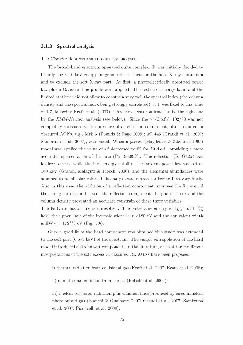
3.1.3 Spectral analysis
The Chandra data were simultaneously analyzed.
The broad–band spectrum appeared quite complex. It was initially decided to
fit only the 3–10 keV energy range in order to focus on the hard X–ray continuum
and to exclude the soft X–ray part. At first, a photoelectrically absorbed power
law plus a Gaussian line profile were applied. The restricted energy band and the
limited statistics did not allow to constrain very well the spectral index (the column
density and the spectral index being strongly correlated), so Γ was fixed to the value
of 1.7, following Kraft et al. (2007). This choice was confirmed to be the right one
by the XMM-Newton analysis (see below). Since the χ2/d.o.f./=102/80 was not
completely satisfactory, the presence of a reflection component, often required in
obscured AGNs, e.g., Mrk 3 (Pounds & Page 2005); 3C 445 (Grandi et al. 2007;
Sambruna et al. 2007), was tested. When a pexrav (Magdziarz & Zdziarski 1995)
model was applied the value of χ2 decreased to 82 for 79 d.o.f., providing a more
accurate representation of the data (PF =99.99%). The reflection (R=Ω/2π) was
let free to vary, while the high–energy cutoff of the incident power law was set at
160 keV (Grandi, Malaguti & Fiocchi 2006), and the elemental abundances were
assumed to be of solar value. This analysis was repeated allowing Γ to vary freely.
Also in this case, the addition of a reflection component improves the fit, even if
the strong correlation between the reflection component, the photon index and the
column density prevented an accurate constrain of these three variables.
The Fe Kα emission line is unresolved. The rest–frame energy is EKα=6.38+0.05−0.06
keV, the upper limit of the intrinsic width is σ <180 eV and the equivalent width
is EWKα=172+84−76 eV (Fig. 3.6).
Once a good fit of the hard component was obtained this study was extended
to the soft part (0.5–3 keV) of the spectrum. The simple extrapolation of the hard
model introduced a strong soft component. In the literature, at least three different
interpretations of the soft excess in obscured RL AGNs have been proposed:
i) thermal radiation from collisional gas (Kraft et al. 2007; Evans et al. 2006);
ii) non–thermal emission from the jet (Belsole et al. 2006);
iii) nuclear scattered radiation plus emission lines produced by circumnuclear
photoionized gas (Bianchi & Guainazzi 2007; Grandi et al. 2007; Sambruna
et al. 2007; Piconcelli et al. 2008).
75

All of these three possibilities were tested.
At first, the soft excess was reproduced with a thermal model (mekal) absorbed
by the Galactic column density. This implicitly assumed that the soft excess is
produced by collisional plasma (with solar abundances). The gas temperature re-
quired by the fit was kT ∼ 0.7, and the model partially reproduced the soft excess,
χ2/d.o.f.=138/104, but the inspection of the residuals still showed excesses below
2 keV. A second mekal was added to verify whether a multi–temperature gas was
present, but the second temperature shifted to an improbable value higher than 10
keV, and excesses were still present in the soft X–ray band (see Fig. 3.4 left panel).
Note that if the abundances are free to vary, they become extremely low, resembling
a power law. After replacing the “second” thermal emission model with a simple
power law (where Γs is free to vary), that represents non–thermal emission, the χ2
improved χ2/d.o.f.=124/103, and the thermal emission was no longer required (the
mekal model is consistent with zero). Although this was the best fit obtained so
far, the model could not reproduce the soft X–ray data completely (Fig. 3.4 right
panel).
Finally the third hypothesis was verified. A soft excess was fitted with a power
law plus emission lines, as expected in case of circumnuclear photoionized gas. The
soft power law slope (Γs) was linked to the hard one (Γh) in order to represent the
scattered nuclear continnum. The fit (see Fig. 3.5 left panel) was very satisfactory
χ2/d.o.f.=103/99. A summary of the best–fit model parameters for the hard X–ray
spectra is given in Table 3.1, while the detected lines and relative significance levels
are listed in Table 3.2.
To obtain an independent confirmation of this result, we explored the XMM-
Newton EPIC spectra. The pn and MOS results were reassuring. All the EPIC
spectra (see Fig.3.5, right panel) were well fitted with the same Chandra best–fit
model. Interestingly, the pn data even required soft lines at the same energies mea-
sured by Chandra.
The pn best–fit model parameters are listed in Tab. 3.3. The relative χ2 is 37.5 for
37 d.o.f.
76
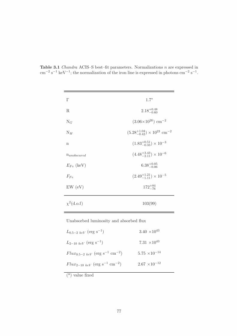
Table 3.1 Chandra ACIS–S best–fit parameters. Normalizations n are expressed incm−2 s−1 keV−1; the normalization of the iron line is expressed in photons cm−2 s−1.
Γ 1.7∗
R 2.18+0.48−0.60
NG (3.06×10²⁰) cm−2
NH (5.28+1.04−0.42) × 1023 cm−2
n (1.83+0.51−0.33) × 10−3
nunobscured (4.48+3.43−2.11) × 10−6
EFe (keV) 6.38+0.05−0.06
FFe (2.49+1.21−1.11) × 10−5
EW (eV) 172+84−76
χ2(d.o.f) 103(99)
Unabsorbed luminosity and absorbed flux
L0.5−2 keV (erg s−1) 3.40 ×1043
L2−10 keV (erg s−1) 7.31 ×1043
Flux0.5−2 keV (erg s−1 cm−2) 5.75 ×10−14
Flux2−10 keV (erg s−1 cm−2) 2.67 ×10⁻¹²
(*) value fixed
77
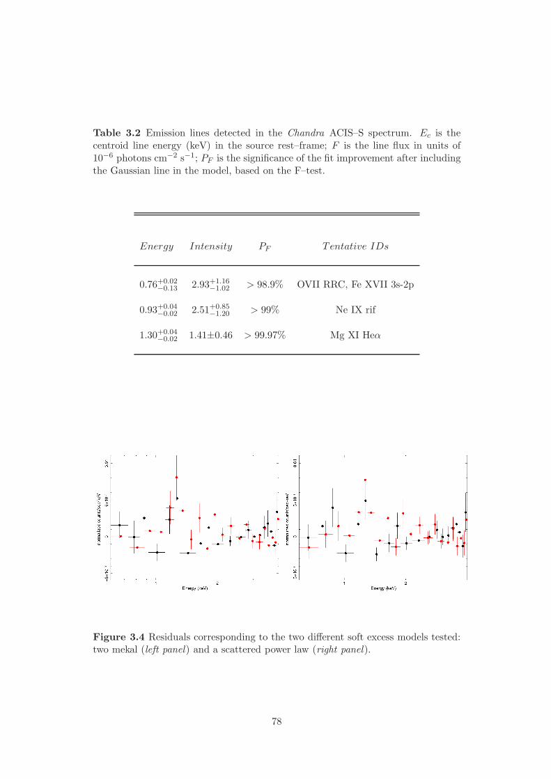
Table 3.2 Emission lines detected in the Chandra ACIS–S spectrum. Ec is thecentroid line energy (keV) in the source rest–frame; F is the line flux in units of10−6 photons cm−2 s−1; PF is the significance of the fit improvement after includingthe Gaussian line in the model, based on the F–test.
Energy Intensity PF Tentative IDs
0.76+0.02−0.13 2.93+1.16
−1.02 > 98.9% OVII RRC, Fe XVII 3s-2p
0.93+0.04−0.02 2.51+0.85
−1.20 > 99% Ne IX rif
1.30+0.04−0.02 1.41±0.46 > 99.97% Mg XI Heα
Figure 3.4 Residuals corresponding to the two different soft excess models tested:two mekal (left panel) and a scattered power law (right panel).
78
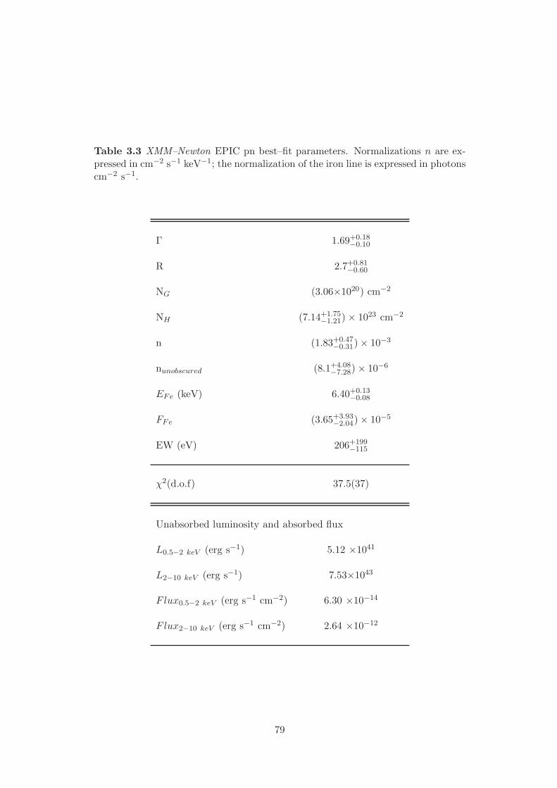
Table 3.3 XMM–Newton EPIC pn best–fit parameters. Normalizations n are ex-pressed in cm−2 s−1 keV−1; the normalization of the iron line is expressed in photonscm−2 s−1.
Γ 1.69+0.18−0.10
R 2.7+0.81−0.60
NG (3.06×10²⁰) cm−2
NH (7.14+1.75−1.21) × 1023 cm−2
n (1.83+0.47−0.31) × 10−3
nunobscured (8.1+4.08−7.28) × 10−6
EFe (keV) 6.40+0.13−0.08
FFe (3.65+3.93−2.04) × 10−5
EW (eV) 206+199−115
χ2(d.o.f) 37.5(37)
Unabsorbed luminosity and absorbed flux
L0.5−2 keV (erg s−1) 5.12 ×1041
L2−10 keV (erg s−1) 7.53×1043
Flux0.5−2 keV (erg s−1 cm−2) 6.30 ×10−14
Flux2−10 keV (erg s−1 cm−2) 2.64 ×10⁻¹²
79
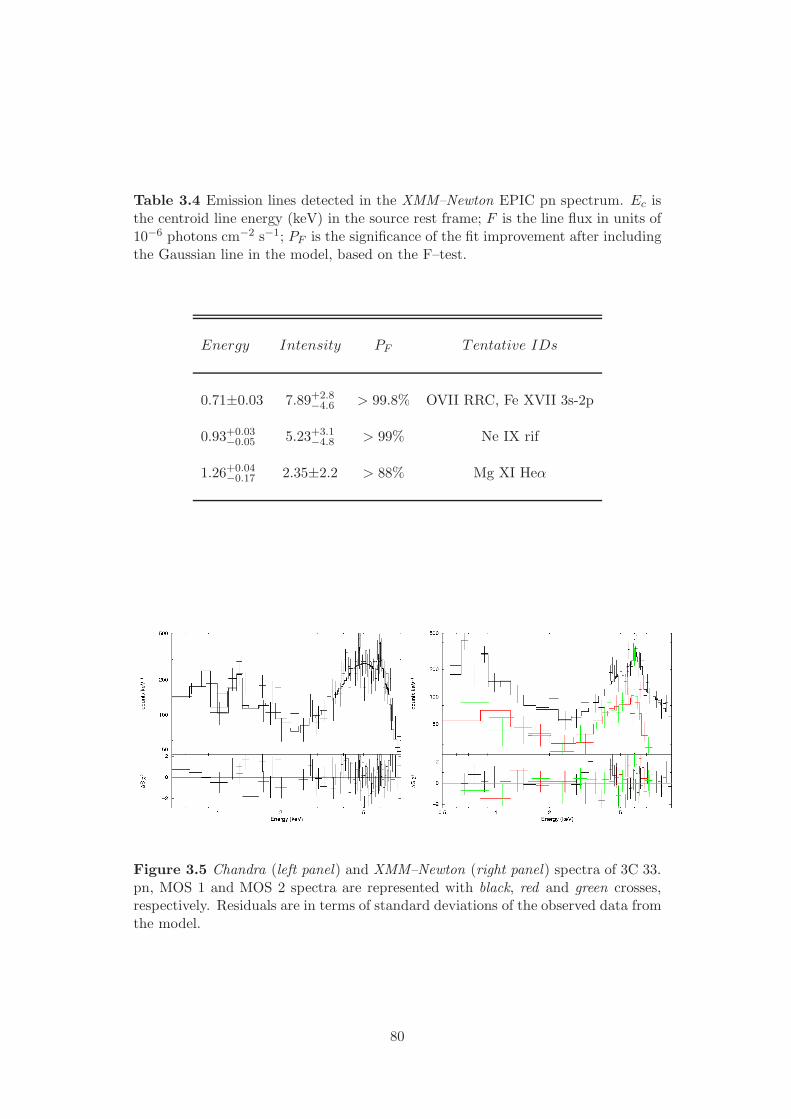
Table 3.4 Emission lines detected in the XMM–Newton EPIC pn spectrum. Ec isthe centroid line energy (keV) in the source rest frame; F is the line flux in units of10−6 photons cm−2 s−1; PF is the significance of the fit improvement after includingthe Gaussian line in the model, based on the F–test.
Energy Intensity PF Tentative IDs
0.71±0.03 7.89+2.8−4.6 > 99.8% OVII RRC, Fe XVII 3s-2p
0.93+0.03−0.05 5.23+3.1
−4.8 > 99% Ne IX rif
1.26+0.04−0.17 2.35±2.2 > 88% Mg XI Heα
Figure 3.5 Chandra (left panel) and XMM–Newton (right panel) spectra of 3C 33.pn, MOS 1 and MOS 2 spectra are represented with black, red and green crosses,respectively. Residuals are in terms of standard deviations of the observed data fromthe model.
80
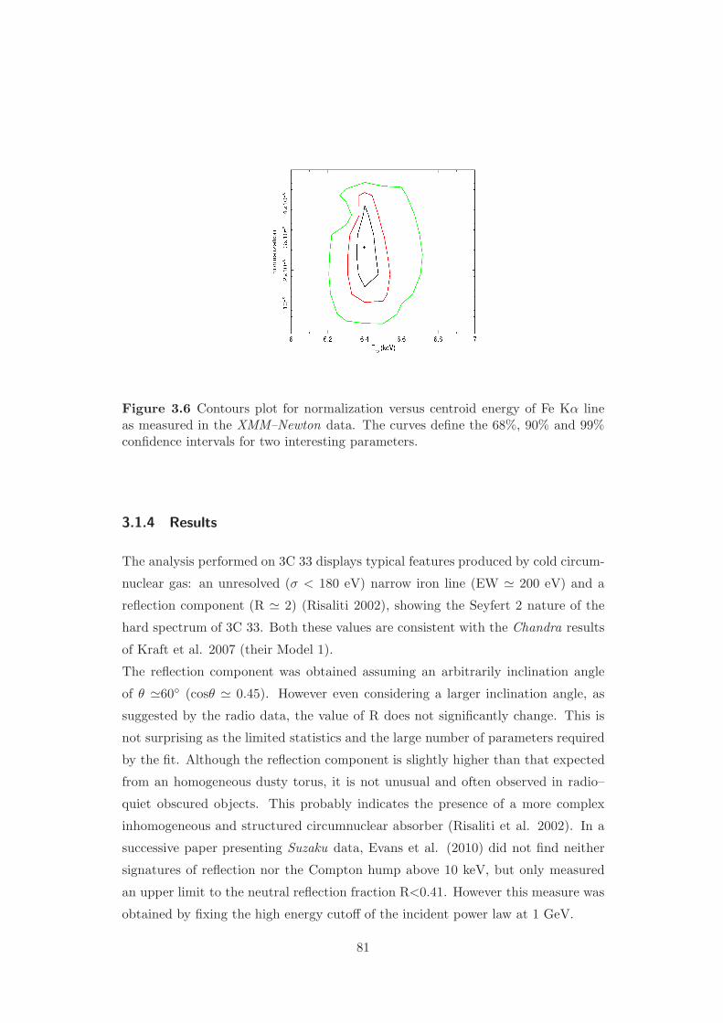
Figure 3.6 Contours plot for normalization versus centroid energy of Fe Kα lineas measured in the XMM–Newton data. The curves define the 68%, 90% and 99%confidence intervals for two interesting parameters.
3.1.4 Results
The analysis performed on 3C 33 displays typical features produced by cold circum-
nuclear gas: an unresolved (σ < 180 eV) narrow iron line (EW ≃ 200 eV) and a
reflection component (R ≃ 2) (Risaliti 2002), showing the Seyfert 2 nature of the
hard spectrum of 3C 33. Both these values are consistent with the Chandra results
of Kraft et al. 2007 (their Model 1).
The reflection component was obtained assuming an arbitrarily inclination angle
of θ ≃60 (cosθ ≃ 0.45). However even considering a larger inclination angle, as
suggested by the radio data, the value of R does not significantly change. This is
not surprising as the limited statistics and the large number of parameters required
by the fit. Although the reflection component is slightly higher than that expected
from an homogeneous dusty torus, it is not unusual and often observed in radio–
quiet obscured objects. This probably indicates the presence of a more complex
inhomogeneous and structured circumnuclear absorber (Risaliti et al. 2002). In a
successive paper presenting Suzaku data, Evans et al. (2010) did not find neither
signatures of reflection nor the Compton hump above 10 keV, but only measured
an upper limit to the neutral reflection fraction R<0.41. However this measure was
obtained by fixing the high energy cutoff of the incident power law at 1 GeV.
81
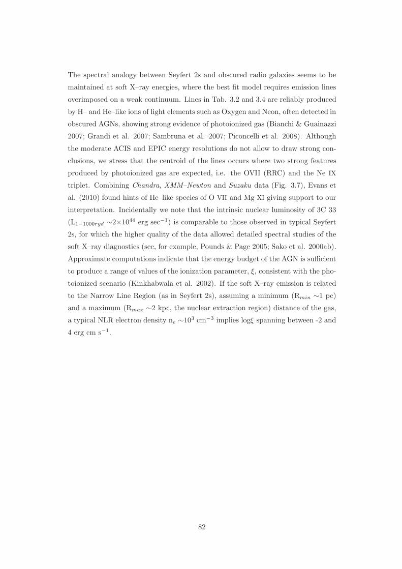
The spectral analogy between Seyfert 2s and obscured radio galaxies seems to be
maintained at soft X–ray energies, where the best fit model requires emission lines
overimposed on a weak continuum. Lines in Tab. 3.2 and 3.4 are reliably produced
by H– and He–like ions of light elements such as Oxygen and Neon, often detected in
obscured AGNs, showing strong evidence of photoionized gas (Bianchi & Guainazzi
2007; Grandi et al. 2007; Sambruna et al. 2007; Piconcelli et al. 2008). Although
the moderate ACIS and EPIC energy resolutions do not allow to draw strong con-
clusions, we stress that the centroid of the lines occurs where two strong features
produced by photoionized gas are expected, i.e. the OVII (RRC) and the Ne IX
triplet. Combining Chandra, XMM–Newton and Suzaku data (Fig. 3.7), Evans et
al. (2010) found hints of He–like species of O VII and Mg XI giving support to our
interpretation. Incidentally we note that the intrinsic nuclear luminosity of 3C 33
(L1−1000ryd ∼2×1044 erg sec−1) is comparable to those observed in typical Seyfert
2s, for which the higher quality of the data allowed detailed spectral studies of the
soft X–ray diagnostics (see, for example, Pounds & Page 2005; Sako et al. 2000ab).
Approximate computations indicate that the energy budget of the AGN is sufficient
to produce a range of values of the ionization parameter, ξ, consistent with the pho-
toionized scenario (Kinkhabwala et al. 2002). If the soft X–ray emission is related
to the Narrow Line Region (as in Seyfert 2s), assuming a minimum (Rmin ∼1 pc)
and a maximum (Rmax ∼2 kpc, the nuclear extraction region) distance of the gas,
a typical NLR electron density ne ∼103 cm−3 implies logξ spanning between -2 and
4 erg cm s−1.
82

Figure 3.7 Combined Chandra, XMM–Newton and Suzaku spectrum of 3C 33in the energy range 0.5–1.5 keV from Evans et al. (2010). The spectral transitionsproduced by the photoionized plasma in the Seyfert 2 galaxy NGC 1068 are reportedas an example.
3.1.5 The origin of the soft X–ray emission
X–ray spectroscopy provides evidence for the presence of soft X–ray emission lines
in the radio galaxy 3C 33.
In spite of the limited spectral power of the ACIS and EPIC cameras features that
are plausibly emitted by a photoionized gas could be detected (see Tab. 3.2 and
Tab. 3.4).
The analogy with Seyfert 2 galaxies is straightforward. Narrow Line Radio Galax-
ies would share similar continua and environments with their RQ counterparts. In
Seyfert 2 galaxies the coincidence in morphology and dimension of the soft X–ray
and the [OIII]λ5007 emission suggests the Narrow Line Region as the location of
such gas. It is then natural to search for a similar X–ray and optical spatial corre-
lation in 3C 33.
For this reason the narrow–band HST ACS/WFC1 optical image, centered at red-
shifted [OIII]λ5007 (filter FR551N), was retrieved from the Multi Mission Archive at
STScI (MAST) 1 and was aligned with the Chandra image as described in Bianchi,
Guainazzi & Chiaberge (2006).
Fig. 3.8 shows the Chandra soft X–ray contours (< 2 keV) superimposed on the
HST [OIII]λ5007 image. The coincidence in extension and morphology between the
1http://archive.stsci.edu/
83
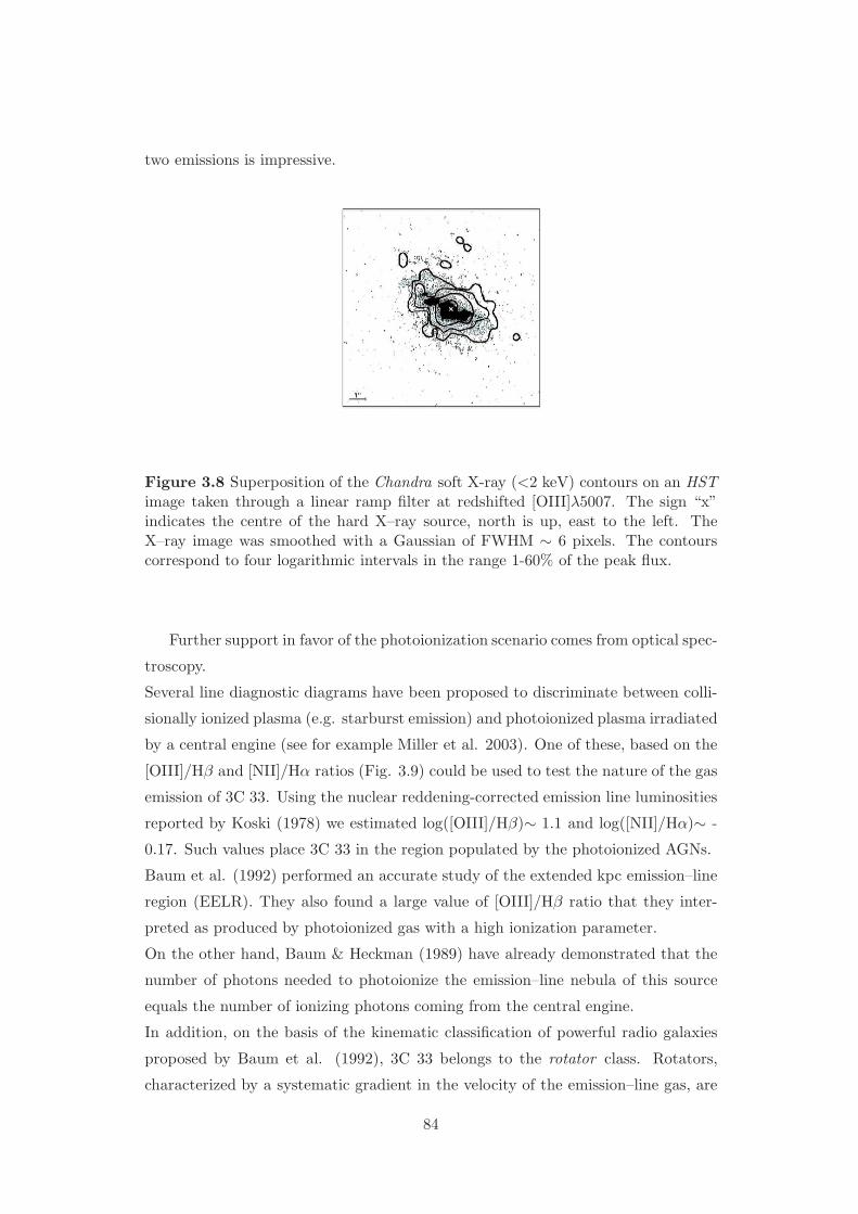
two emissions is impressive.
Figure 3.8 Superposition of the Chandra soft X-ray (<2 keV) contours on an HSTimage taken through a linear ramp filter at redshifted [OIII]λ5007. The sign “x”indicates the centre of the hard X–ray source, north is up, east to the left. TheX–ray image was smoothed with a Gaussian of FWHM ∼ 6 pixels. The contourscorrespond to four logarithmic intervals in the range 1-60% of the peak flux.
Further support in favor of the photoionization scenario comes from optical spec-
troscopy.
Several line diagnostic diagrams have been proposed to discriminate between colli-
sionally ionized plasma (e.g. starburst emission) and photoionized plasma irradiated
by a central engine (see for example Miller et al. 2003). One of these, based on the
[OIII]/Hβ and [NII]/Hα ratios (Fig. 3.9) could be used to test the nature of the gas
emission of 3C 33. Using the nuclear reddening-corrected emission line luminosities
reported by Koski (1978) we estimated log([OIII]/Hβ)∼ 1.1 and log([NII]/Hα)∼ -
0.17. Such values place 3C 33 in the region populated by the photoionized AGNs.
Baum et al. (1992) performed an accurate study of the extended kpc emission–line
region (EELR). They also found a large value of [OIII]/Hβ ratio that they inter-
preted as produced by photoionized gas with a high ionization parameter.
On the other hand, Baum & Heckman (1989) have already demonstrated that the
number of photons needed to photoionize the emission–line nebula of this source
equals the number of ionizing photons coming from the central engine.
In addition, on the basis of the kinematic classification of powerful radio galaxies
proposed by Baum et al. (1992), 3C 33 belongs to the rotator class. Rotators,
characterized by a systematic gradient in the velocity of the emission–line gas, are
84

nearly always associated with powerful radio sources (Lradio ≥1042 erg s−1) having
luminous high–ionization nuclear emission–line region.
The kinematic study of the gas also shows that the gas rotation axis and the radio
axis are aligned within 10 (Baum et al. 1992). Moreover the rotation axis of the
gas is not aligned with the stellar rotation axis (Heckman et al. 1985), disfavoring
the hypothesis of a collisional (starburst) gas emission.
Figure 3.9 Line diagnostic diagram from Miller et al. (2003). It is used to differen-tiate AGNs (red circles) from star–forming galaxies (blue triangles). The solid linerepresents the 1σ lower limit of the model from Kewley et al. (2001). The estimatedvalues log([OIII]/Hβ)∼ 1.1 and log([NII]/Hα)∼ -0.17 from Koski (1978) place 3C 33largely in the AGN region (red cross).
3.1.6 Summary
The X–ray analysis of the Narrow Line Radio Galaxy 3C 33 confirms the Seyfert
2 nature of this source. In agreement with previous works the complexity of the
broad–band spectrum, largely dominated by strong obscuration (NH ∼1023 cm−2),
is confirmed.
A prominent Fe Kα line at 6.4 keV is also present. Its EW of ∼ 200 eV is in
agreement with being produced by optically–thick circumnuclear matter (Ghisellini
Haardt & Matt 1994).
The soft excess has been interpreted as emitting gas photoionized by the central en-
gine. There are several clues favoring this hypothesis. First of all both Chandra and
XMM–Newton soft X–ray spectra can be better fit with an unobscured scattered
85
power law plus highly ionized lines, rather than with one or more thermal compo-
nents. Next, a rough estimate of the ionization parameter ξ, expected in the case
that the emitting line gas is located in the NLR, is consistent with a photoionized
scenario, and finally there is a remarkable spatial coincidence between the extended
soft X–ray and the [OIII]λ5007 emission.
X–ray findings are also consistent with pieces of evidence coming from other wave-
lengths. The optical line ratios [OIII]/Hβ and [NII]/Hα put 3C 33 among the AGNs,
far away from the region populated by starburst galaxies in the diagnostic plane of
Miller et al. (2003). The extended kpc emission line region has a line–rich optical
spectrum with large [OIII]/Hβ ratio, typical of photoionized gas. Moreover the
estimated photons required to photoionize the emission–line nebula (in the optical
band) are provided entirely by the nuclear engine.
The kinematical properties of the extended gas of 3C 33, based on optical spec-
troscopy, are typical of powerful radio galaxies with high–ionization nuclear emis-
sion. The gas rotation axis and the radio axis are aligned within 10, but the former
is not aligned with the stellar rotation axis.
All together these results seem to draw a photoionized scenario for the circumnuclear
environment implying that radiative processes are still at work on kpc distances and
could compete with the jet kinetic power (see Chapter 5). Another important im-
plication is that RL and RQ AGNs seem to share similar environment properties
and consequently, similar accretion mechanisms can be present in high–luminosity
AGNs, indipendently on the presence/absence of powerful extended jets.
86
4Warm photoionized gas in
absorption
4.1 Introduction
The first suggestion of an X–ray warm absorber (WA), i.e., absorption by ionized
gas in our line–of–sight, was made by Halpern (1984) with the EXOSAT satellite on
the QSO MR2251–158. It is now well established that at least half of all Seyfert 1s
is characterized by photoionized warm absorption (Blustin et a. 2005; McKernan et
al. 2007). High–resolution spectroscopic data (RGS, HETG, LETG) dramatically
improved our knowledge of WAs. The application of detailed photoionized codes
(see next Section) revealed that quite often the gas is stratified, with a wide range
in ionization parameter ξ (see Chapter 2) and column densities, ranging between
1020−23 cm−2, with velocities of the order of a few hundreds to thousands km s−1
(Blustin et al. 2005; McKernan et al. 2007). Where these winds originate and are
powered is still an open question. Several regions at different distances from the
central engine, like the NLR, the obscuring torus and the accretion disk have been
proposed as a possible location for the gas (Crenshaw et al. 2003; Krolik & Kriss
2001; Proga & Kallman 2004).
As discussed in Chapter 5, soft X–ray WAs in Seyferts have kinetic luminosities that
account for less than 1% the bolometric luminosity (Blustin et al. 2005). Therefore,
it seems that they are not playing a fundamental role in the general picture of the
AGN feedback. The situation changes when extreme WAs are considered. These
87
outflows can reach velocities of ∼0.1c–0.3c, and consequently their kinetic lumi-
nosities can compete with the accretion luminosities. Such winds could represent a
driving mechanism for the feedback processes (Gofford et al. 2011 and references
therein).
If the presence of X–ray absorbing gas is well established in Seyfert 1s, for RL
AGNs the investigation of the nuclear environment through high–resolution spec-
troscopy has just started. Therefore, detections of WAs in type 1 objects, i.e.,
BLRGs, are still a handful. BLRGs are complex objects. The Doppler amplifica-
tion of the jet emission can play a key role in dimming the spectral features. For
example, RGs are known to have weaker Compton reflection signatures and weaker
Fe Kα lines when compared to Seyfert 1s (Grandi, Malaguti & Fiocchi 2006 and
references therein). Up to now, controversial hints of WAs have been observed in
the past in a handful of RL sources: 3C 382 and 3C 390.3 with ASCA (Reynolds
1997); 3C 351 with ROSAT PSPC (Nicastro et al. 1999); 4C+74.26 with the XMM–
Newton EPIC cameras (Ballantyne 2005).
It is unclear whether winds can form and/or survive in the nuclear regions of RL
AGNs, where large amounts of the gravitational power is funneled into relativistic
collimated plasma. Addressing this point is fundamental to clarify the physical link
among accretion flows, winds and jet, and the influence that each of these compo-
nents can have on the host galaxy.
4.2 Warm absorber modelling
To understand the physical properties of a warm absorbing gas, plasma codes that
calculate the output spectrum from a cloud of photoionized gas, are required. There
are several plasma codes available, such as XSTAR 1, SPEX 2, CLOUDY 3, Titan 4,
Mocassin 5.
In this thesis I concentrate on XSTAR and SPEX. In particular, the first one is used
to model the 3C 382 WA, while the latter is employed in fitting 3C 390.3 and 3C 120
RGS spectra.
1http://heasarc.nasa.gov/lheasoft/xstar/xstar.html2http://www.sron.nl/spex3http://www.nublado.org4http://Vo.obspm.fr/simulation5http://hea-www.harvard.edu/ bercolano
88
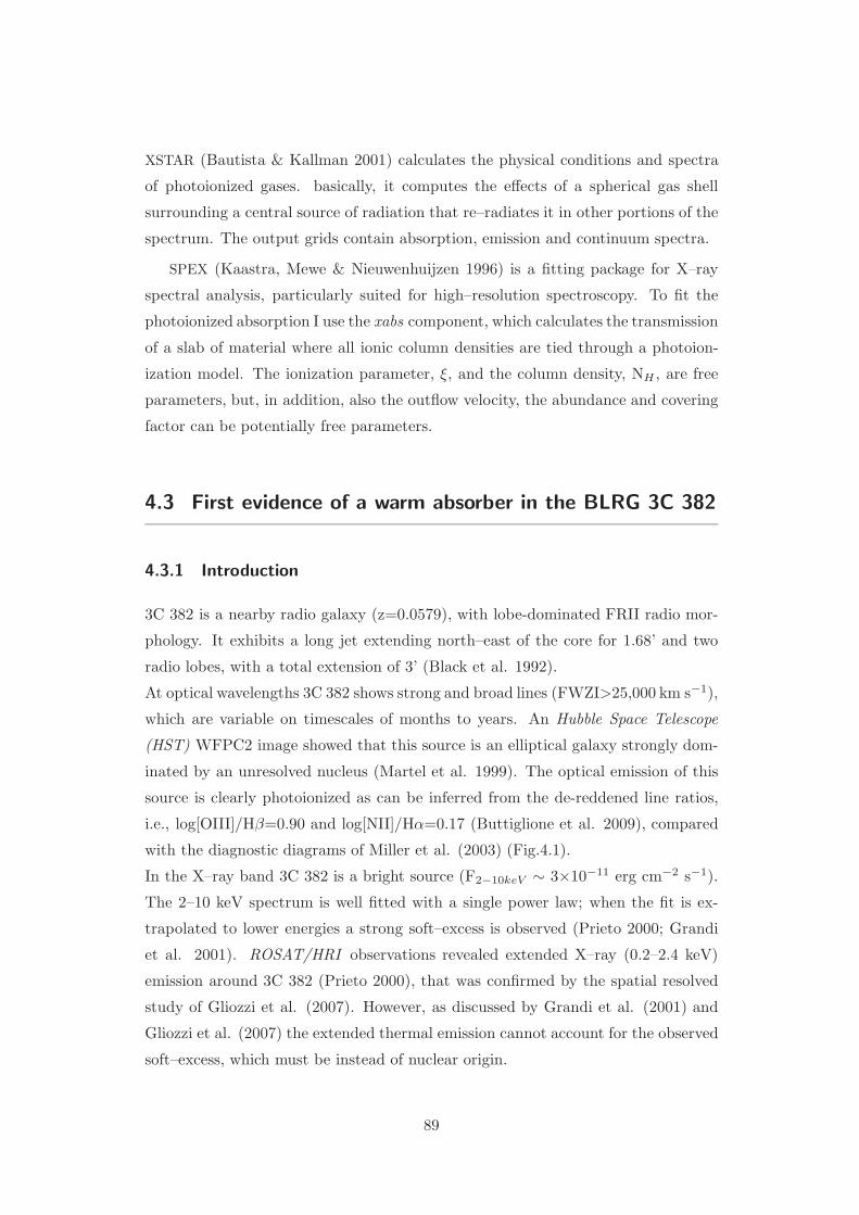
XSTAR (Bautista & Kallman 2001) calculates the physical conditions and spectra
of photoionized gases. basically, it computes the effects of a spherical gas shell
surrounding a central source of radiation that re–radiates it in other portions of the
spectrum. The output grids contain absorption, emission and continuum spectra.
SPEX (Kaastra, Mewe & Nieuwenhuijzen 1996) is a fitting package for X–ray
spectral analysis, particularly suited for high–resolution spectroscopy. To fit the
photoionized absorption I use the xabs component, which calculates the transmission
of a slab of material where all ionic column densities are tied through a photoion-
ization model. The ionization parameter, ξ, and the column density, NH , are free
parameters, but, in addition, also the outflow velocity, the abundance and covering
factor can be potentially free parameters.
4.3 First evidence of a warm absorber in the BLRG 3C 382
4.3.1 Introduction
3C 382 is a nearby radio galaxy (z=0.0579), with lobe-dominated FRII radio mor-
phology. It exhibits a long jet extending north–east of the core for 1.68’ and two
radio lobes, with a total extension of 3’ (Black et al. 1992).
At optical wavelengths 3C 382 shows strong and broad lines (FWZI>25,000 km s−1),
which are variable on timescales of months to years. An Hubble Space Telescope
(HST) WFPC2 image showed that this source is an elliptical galaxy strongly dom-
inated by an unresolved nucleus (Martel et al. 1999). The optical emission of this
source is clearly photoionized as can be inferred from the de-reddened line ratios,
i.e., log[OIII]/Hβ=0.90 and log[NII]/Hα=0.17 (Buttiglione et al. 2009), compared
with the diagnostic diagrams of Miller et al. (2003) (Fig.4.1).
In the X–ray band 3C 382 is a bright source (F2−10keV ∼ 3×10⁻¹¹ erg cm−2 s−1).
The 2–10 keV spectrum is well fitted with a single power law; when the fit is ex-
trapolated to lower energies a strong soft–excess is observed (Prieto 2000; Grandi
et al. 2001). ROSAT/HRI observations revealed extended X–ray (0.2–2.4 keV)
emission around 3C 382 (Prieto 2000), that was confirmed by the spatial resolved
study of Gliozzi et al. (2007). However, as discussed by Grandi et al. (2001) and
Gliozzi et al. (2007) the extended thermal emission cannot account for the observed
soft–excess, which must be instead of nuclear origin.
89
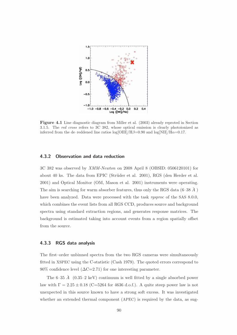
Figure 4.1 Line diagnostic diagram from Miller et al. (2003) already reproted in Section3.1.5. The red cross refers to 3C 382, whose optical emission is clearly photoionized asinferred from the de–reddened line ratios log[OIII]/Hβ=0.90 and log[NII]/Hα=0.17.
4.3.2 Observation and data reduction
3C 382 was observed by XMM-Newton on 2008 April 8 (OBSID: 0506120101) for
about 40 ks. The data from EPIC (Struder et al. 2001), RGS (den Herder et al.
2001) and Optical Monitor (OM, Mason et al. 2001) instruments were operating.
The aim is searching for warm absorber features, thus only the RGS data (6–38 A )
have been analyzed. Data were processed with the task rgsproc of the SAS 8.0.0,
which combines the event lists from all RGS CCD, produces source and background
spectra using standard extraction regions, and generates response matrices. The
background is estimated taking into account events from a region spatially offset
from the source.
4.3.3 RGS data analysis
The first–order unbinned spectra from the two RGS cameras were simultaneously
fitted in XSPEC using the C-statistic (Cash 1979). The quoted errors correspond to
90% confidence level (∆C=2.71) for one interesting parameter.
The 6–35 A (0.35–2 keV) continuum is well fitted by a single absorbed power
law with Γ = 2.25 ± 0.18 (C=5264 for 4636 d.o.f.). A quite steep power law is not
unexpected in this source known to have a strong soft excess. It was investigated
whether an extended thermal component (APEC) is required by the data, as sug-
90
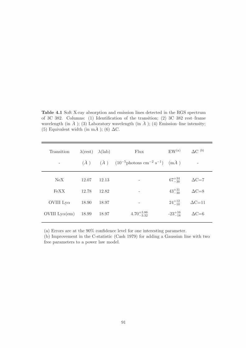
Table 4.1 Soft X-ray absorption and emission lines detected in the RGS spectrumof 3C 382. Columns: (1) Identification of the transition; (2) 3C 382 rest–framewavelength (in A ); (3) Laboratory wavelength (in A ); (4) Emission–line intensity;(5) Equivalent width (in mA ); (6) ∆C.
Transition λ(rest) λ(lab) Flux EW(a) ∆C (b)
- (A ) (A ) (10−5photons cm−2 s−1) (mA ) -
NeX 12.07 12.13 - 67+34−30 ∆C=7
FeXX 12.78 12.82 - 43+31−30 ∆C=8
OVIII Lyα 18.90 18.97 - 24+12−10 ∆C=11
OVIII Lyα(em) 18.99 18.97 4.70+3.86−3.32 -23+16
−18 ∆C=6
(a) Errors are at the 90% confidence level for one interesting parameter.(b) Improvement in the C-statistic (Cash 1979) for adding a Gaussian line with twofree parameters to a power law model.
91

gested by the Chandra analysis. The fit did not improve significantly, nor did the
shape of the residuals (C=5261), therefore it is not included.
At first a phenomenological approach was adopted. The spectra were divided
into a number of regions containing about the same number of bins each (100). An
accurate inspection of every single region was performed. Where the spectra showed
a particularly evident absorption feature, a Gaussian profile with 0–width and a
negative normalization was added to the model. Only lines yielding an improvement
in the fit higher than ∆C>5 (corresponding to > 95% for two interesting parameters)
were taken into account. For these structures the equivalent width was estimated
and the corresponding atomic transition identified through several atomic databases
such as CHIANTI (Dere et al. 1997; Landi et al. 2006), ATOMDB WebGUIDE 6 and
NIST 7. The parameters of the most prominent lines are reported in Table 4.1 and
the phenomenological fit is shown in Fig.4.2. Two other absorption lines probably
corresponding to FeXXI/MgXI and SIV/NVII transitions, although observed, are
not reported in Table 4.1 because of their marginal detection (∆C =5). None of the
detected features is due to local (Galactic) absorption.
Finally, an emission line identified as OVIII Lyα was clearly detected with ∆C=6
(see Table 4.1). Emission features are often observed in sources showing signatures
of warm absorber (Blustin et al. 2002; Turner et al. 2004).
Once the presence of absorption lines was ascertained via the phenomenological
analysis, the next step was to study the physical properties of the gas using a self
consistent modeling of the spectrum. Extensive simulations were carried out using
the photoionization code XSTAR (v2.1ln9). The output was a grid of models (after-
wards simply called XSTAR model) that can be fitted to the data in XSPEC. Each
model in the grid represents a photoionized spectrum characterized by a particular
value of the column density and the ionization parameter. The explored parameter
range is NH=[1018, 1023] and logξ=[-3, 3]. A simple spherical geometry for the
illuminated gas (covering factor =1), solar abundances (Grevesse & Sauval 1998) ,
and an illuminating continuum from 1 to 1000 Rydbergs derived from the intrinsic
spectral energy distribution SED of the source (Fig.4.3 and Tab. 5.1) were assumed.
The turbulent velocity of the gas was set to vturb=100 km s−1, as the limited RGS
statistics did not allow to constrain the intrinsic width of the absorption features.
The XSTAR model obtained from these simulations was applied as an XSPEC
multiplicative component to the power law and fitted to the data. The fit signifi-
6http://cxc.harvard.edu/atomdb/WebGUIDE/index.html7http://physics.nist.gov
92
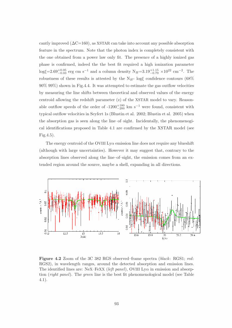
cantly improved (∆C=160), as XSTAR can take into account any possible absorption
feature in the spectrum. Note that the photon index is completely consistent with
the one obtained from a power law only fit. The presence of a highly ionized gas
phase is confirmed, indeed the the best fit required a high ionization parameter
logξ=2.69+0.05−0.03 erg cm s−1 and a column density NH=3.19+1.15
−0.79 ×1022 cm−2. The
robustness of these results is attested by the NH - logξ confidence contours (68%
90% 99%) shown in Fig.4.4. It was attempted to estimate the gas outflow velocities
by measuring the line shifts between theoretical and observed values of the energy
centroid allowing the redshift parameter (z) of the XSTAR model to vary. Reason-
able outflow speeds of the order of -1200+180−200 km s−1 were found, consistent with
typical outflow velocities in Seyfert 1s (Blustin et al. 2002; Blustin et al. 2005) when
the absorption gas is seen along the line–of–sight. Incidentally, the phenomenogi-
cal identifications proposed in Table 4.1 are confirmed by the XSTAR model (see
Fig.4.5).
The energy centroid of the OVIII Lyα emission line does not require any blueshift
(although with large uncertainties). However it may suggest that, contrary to the
absorption lines observed along the line–of–sight, the emission comes from an ex-
tended region around the source, maybe a shell, expanding in all directions.
Figure 4.2 Zoom of the 3C 382 RGS observed–frame spectra (black : RGS1; red :RGS2), in wavelength ranges, around the detected absorption and emission lines.The identified lines are: NeX–FeXX (left panel), OVIII Lyα in emission and absorp-tion (right panel). The green line is the best fit phenomenological model (see Table4.1).
93

Figure 4.3 Radio to X–ray spectral energy distribution of 3C 382. Data are fromliterature (Rudnick et al. 1986; Knapp et al. 1990; Klavel et al. 2000; Lilly &Longair 1982; Chiaberge et al. 2000; Chiaberge et al. 2002; Grandi et al. 2001;Quillen et al. 2003; Ramos Almeida et al. 2007; Hinshaw et al. 2007). Optical andUV measurements de–reddened with the extinction curve of Cardelli et al. (1989).The visual extinction is deduced by the Galactic column density, assuming the gas–to–dust ratio from Shull et al. (1985).
Figure 4.4 Contour plots for column density and ionization parameter values ofthe 3C 382 warm absorber as obtained with the XSTAR model. The curves definethe 68%, 90% and 99% confidence intervals for two interesting parameters.
94
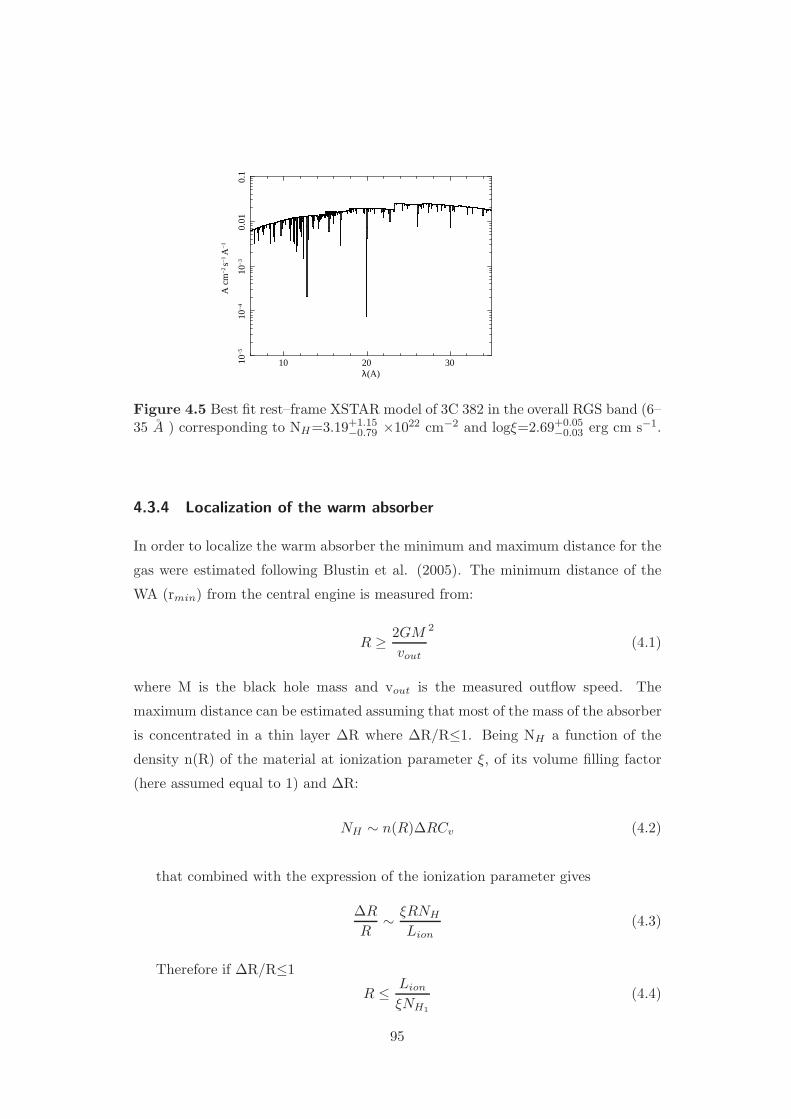
10 20 3010−
510
−4
10−
30.
010.
1
A c
m−
2 s−
1 A
−1
λ(A)
Figure 4.5 Best fit rest–frame XSTAR model of 3C 382 in the overall RGS band (6–35 A ) corresponding to NH=3.19+1.15
−0.79 ×1022 cm−2 and logξ=2.69+0.05−0.03 erg cm s−1.
4.3.4 Localization of the warm absorber
In order to localize the warm absorber the minimum and maximum distance for the
gas were estimated following Blustin et al. (2005). The minimum distance of the
WA (rmin) from the central engine is measured from:
R ≥2GM
vout
2
(4.1)
where M is the black hole mass and vout is the measured outflow speed. The
maximum distance can be estimated assuming that most of the mass of the absorber
is concentrated in a thin layer ∆R where ∆R/R≤1. Being NH a function of the
density n(R) of the material at ionization parameter ξ, of its volume filling factor
(here assumed equal to 1) and ∆R:
NH ∼ n(R)∆RCv (4.2)
that combined with the expression of the ionization parameter gives
∆R
R∼
ξRNH
Lion(4.3)
Therefore if ∆R/R≤1
R ≤Lion
ξNH1
(4.4)
95
The BLR radius can be calculated as (Ghisellini & Tavecchio 2008):
RBLR = 1017L1/2disk,45cm (4.5)
and the torus radius as (Cleary et al. 2007):
Rtorus = 2.5 × 10¹⁸L1/2disk,45cm (4.6)
For 3C 382 it was possible to estimate the location of the gas between 10 and
60 pc. Given the BLR and torus radii as RBLR ≃0.06 pc and Rtorus ≃1.5 pc if
Ldisk ∼ Lion (see Table 5.2), these results suggest that the bulk of the highly ionized
absorption gas, detected in 3C 382, is located beyond the torus, most likely in the
NLR. Interestingly, this is also the probable location of the photoionized emitting
gas observed in 3C 33 (Chapter 3). However, the estimation of the maximum
distance of the absorber depends also on the volume filling factor, thus for smaller
values of Cv the distance of the gas reduces (see Chapter 5). A re–analysis of the
HETG data of 3C 382 (Reeves et al. 2009) confirmed these results.
4.3.5 Summary
The high–resolution analysis of the BLRG 3C 382 has revealed that relativistic col-
limated plasma and slower outflows of photoionized gas can coexist in the same
object. The outflowing gas is found in a hot phase as attested by the derived ion-
ization parameter logξ=2.69 erg cm s−1 deduced from XSTAR simulations. Most
of the light elements are indeed completely ionized, and the strongest absorption
features correspond to H–like elements and L–shell iron states. In Seyfert 1s warm
absorbers are complex and multi–phase, often indicating that layers of gas at dif-
ferent ionization states are part of the same outflow (Blustin et al. 2005). In the
present case, only one zone of hot gas was observed, without apparent traces of a
colder component. Nonetheless, the physical conditions of the gas in 3C 382 warm
absorber are quite similar to those measured in the highest ionized absorber in their
radio–quiet counterparts (NGC 4051, Krongold et al. 2007; Mkr 279, Costantini
et al. 2007; IRAS13349+2438, Sako et al. 2001). Taking into account the short
exposure time and the very simple assumptions in the XSTAR model, the result
appears encouraging. It is worth noting that setting vturb to an a priori fixed value
could potentially overpredict the column density if the real turbulent velocity is
larger. Interestingly, also the EWs of the absorption lines detected in 3C 382 are
96
consistent with those generally measured in Seyfert 1s (Yaqoob et al. 2003; Turner
et al. 2004). This similarity suggests a negligible jet contribution to the soft X–
ray spectrum, although the large uncertainties in EW prevent more quantitative
statements from being made.
4.4 Warm Absorbers in other BLRGs
4.4.1 Introduction
After the results of 3C 382, that confirm for the first time the presence of absorption
features in a RL AGN, I turned my attention to other BLRGs. The aim was to
check if warm absorbers are typical stuctures of RL AGNs as it occurs Seyfert 1s.
In particular I focussed on 3C 390.3 and 3C 120, the only two BLRGs with available
data in the public archives, with exposure time long enough (texp ∼50 ks) to allow
the analysis of the RGS spectra.
3C 390.3 (z=0.0561; Hewitt & Burbidge 1991) is a classical double–lobed FRII
radio galaxy (Pearson & Readhead 1988). It is one of the closest radio sources
whose core exhibits superluminal motion in the pc–scale jet (Alef et al. 1996).
From the apparent velocity of 3.5c and the core dominance, Giovannini et al. (2001)
estimated a jet inclination angle 30 < θ < 35 with β ∼0.96–0.99. Double–peaked
emission lines characterize the otpical and UV spectra of the source (Eracleous &
Halpern 1994; Zheng 1996; Wamsteker et al. 1997), while the UV bump is weak
or even absent (Wamsteker et al. 1997). 3C 390.3 is known to be variable in
the X–ray band, with variations in both soft and hard band on timescale of weeks
to months (Leighly & O’Brien 1997; Gliozzi et al. 2003). All previous X–ray
telescopes observed this source. While in the hard X–ray band there is a general
agreement on the presence of an iron line and reflection hump (Grandi et al. 1999;
Sambruna et al. 2009), the modelization of the soft X–ray band is controversial.
Einstein–IPC (Kruper et al. 1990) and BeppoSAX (Grandi et al. 1999) required an
excess of column density. EXOSAT claimed the presence of a soft excess (Ghosh &
Sondararajaperumal 1991) while Reynolds (1997) found hints of warm absorption
in the ASCA data, successively confirmed by the detection of an absorption edge
at 0.65 keV (Sambruna et al. 1999). Recently Sambruna et al. (2009) observed
an emission line in the RGS spectrum associated with O VII forbidden possibly
produced in the NLR.
97
3C 120 (z=0.033; Burbidge 1967) is classified as a FRI exhibiting a one–sided jet
(Seielstad et al. 1979; Walker et al. 1987; Harris et al. 2004). The apparent trans-
verse velocity of the jet vapp=5.3c, as obtained by the VLBA observation (Lister et
al. 2009), implies an upper limit for the inclination angle of 21. The optical spec-
trum of 3C 120 is typical of Seyfert 1 galaxies, with strong and broad emission lines,
quite unusual for FRI radio sources. Reverbation mapping constrains the black hole
mass to be 5.5+3.1−2.3×10⁷ M⊙ (Peterson et al. 2004). At UV wavelenghts, 3C 120 has
a typical AGN spectrum with a strong blue bump and strong emission lines signa-
ture of a standard optically–thick geometrically–thin accretion disk (Maraschi et al.
1991). The hard X–ray spectrum is characterized by a slightly broadened iron line
(EW∼100 eV) at 6.4 keV, a weak ionized line at 6.9 keV (Yaqoob & Padmanabhan
2004; Kataoka et al. 2007) and Compton reflection Ω/2π∼0.4–0.5 (Eracleous et al.
2000; Zdziarski & Grandi 2001; Gliozzi et al. 2003; Ballantyne et al. 2004). The
soft X–ray band of 3C 120 has been observed by the grating instruments onboard
Chandra and XMM–Newton. In the Chandra High Energy Transmission Gratings
(HETGs) spectrum an O VIII Lyα absorption line blueshifted by ∼ -5500 km s−1
was observed (McKernan et al. 2003). This feature was not revealed by the XMM–
Newton/RGS (Ogle et al. 2005) that on the contrary shows a slighlty redshifted O
VIII emission structure.
4.4.2 Data analysis
3C 390.3 was observed by XMM–Newton/RGS (den Herder et al. 2001) on 2004
October 8–9 for a total exposure of 50 ks and on October 17 for 20 ks.
3C 120 was pointed twice, on 2002 September 6 for 12 ks and on 2003 August
26 for 130 ks. In order to have a good S/N ratio, here only the second and longer
observation is considered. The RGS1 and RGS2 spectra were extracted using the
SAS V9.0 task rgsproc, which combines the event lists from all RGS CCD, produces
source and background spectra using a region spatially offset from that containing
the source, and generates response matrices. The resulting spectra were analyzed
using the fitting package SPEX. The Galactic absorption was modeled with the SPEX
HOT component. For all spectral models Solar elemental abundances were adopted
(Anders & Grevesse 1989). For each source the proper line–of–sight Galactic column
density was considered, NH=3.5×1020 cm−2 and NH=1.1×1021 cm−2 for 3C 390.3
and 3C 120, respectively (Kalberla et al. 2005). A slightly different cosmology was
98
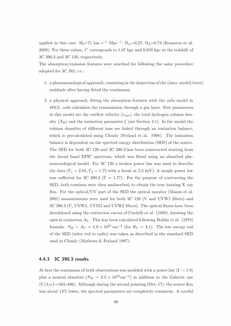
applied in this case: H0=71 km s−1 Mpc−1, Ωm=0.27, ΩΛ=0.73 (Komatsu et al.
2009). For these values, 1” corresponds to 1.07 kpc and 0.650 kpc at the redshift of
3C 390.3 and 3C 120, respectively.
The absorption/emission features were searched for following the same procedure
adopted for 3C 382, i.e.:
1. a phenomenological approach, consisting in the inspection of the (data–model/error)
residuals after having fitted the continuum;
2. a physical approach, fitting the absorption features with the xabs model in
SPEX. xabs calculates the transmission through a gas layer. Free parameters
in this model are the outflow velocity (vout), the total hydrogen column den-
sity (NH) and the ionization parameter ξ (see Section 4.1). In the model the
column densities of different ions are linked through an ionization balance,
which is precalculated using Cloudy (Ferland et al. 1998). The ionization
balance is dependent on the spectral energy distribution (SED) of the source.
The SED for both 3C 120 and 3C 390.3 has been constructed starting from
the broad band EPIC spectrum, which was fitted using an absorbed phe-
nomenological model. For 3C 120 a broken power law was used to describe
the data (Γ1 = 2.04, Γ2 = 1.75 with a break at 2.5 keV). A simple power law
was sufficient for 3C 390.3 (Γ = 1.77). For the purpose of contructing the
SED, both continua were then unabsorbed, to obtain the true ionizing X–ray
flux. For the optical/UV part of the SED the optical monitor (Mason et al.
2001) measurements were used for both 3C 120 (V and UVW1 filters) and
3C 390.3 (U, UVW1, UVM2 and UVW2 filters). The optical fluxes have been
dereddened using the extinction curves of Cardelli et al. (1989), knowing the
optical extinction AV . This has been calculated following Bohlin et al. (1978)
formula: NH ∼ AV = 1.9 × 1021 cm−2 (for RV = 3.1). The low energy tail
of the SED (infra–red to radio) was taken as described in the standard SED
used in Cloudy (Mathews & Ferland 1987).
4.4.3 3C 390.3 results
At first the continuum of both observations was modeled with a power law (Γ ∼ 1.9)
plus a neutral absorber (NH ∼ 2.5 × 1020cm−2) in addition to the Galactic one
(C/d.o.f.=583/406). Although during the second pointing (Oct. 17), the source flux
was about 14% lower, the spectral parameters are completely consistent. A careful
99
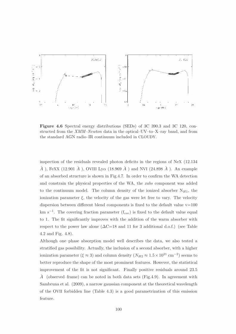
Figure 4.6 Spectral energy distributions (SEDs) of 3C 390.3 and 3C 120, con-structed from the XMM–Newton data in the optical–UV–to–X–ray band, and fromthe standard AGN radio–IR continuum included in CLOUDY.
inspection of the residuals revealed photon deficits in the regions of NeX (12.134
A ), FeXX (12.901 A ), OVIII Lyα (18.969 A ) and NVI (24.898 A ). An example
of an absorbed structure is shown in Fig.4.7. In order to confirm the WA detection
and constrain the physical properties of the WA, the xabs component was added
to the continuum model. The column density of the ionized absorber NH1, the
ionization parameter ξ, the velocity of the gas were let free to vary. The velocity
dispersion between different blend components is fixed to the default value v=100
km s−1. The covering fraction parameter (fcov) is fixed to the default value equal
to 1. The fit significantly improves with the addition of the warm absorber with
respect to the power law alone (∆C=18 and 11 for 3 additional d.o.f.) (see Table
4.2 and Fig. 4.8).
Although one–phase absorption model well describes the data, we also tested a
stratified gas possibility. Actually, the inclusion of a second absorber, with a higher
ionization parameter (ξ ≈ 3) and column density (NH2 ≈ 1.5×1021 cm−2) seems to
better reproduce the shape of the most prominent features. However, the statistical
improvement of the fit is not significant. Finally positive residuals around 23.5
A (observed–frame) can be noted in both data sets (Fig.4.9). In agreement with
Sambruna et al. (2009), a narrow gaussian component at the theoretical wavelength
of the OVII forbidden line (Table 4.3) is a good parametrization of this emission
feature.
100
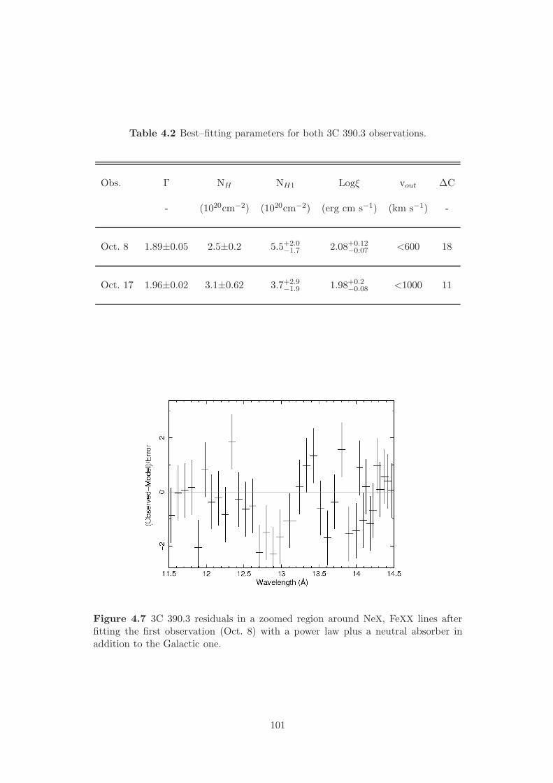
Table 4.2 Best–fitting parameters for both 3C 390.3 observations.
Obs. Γ NH NH1 Logξ vout ∆C
- (1020cm−2) (1020cm−2) (erg cm s−1) (km s−1) -
Oct. 8 1.89±0.05 2.5±0.2 5.5+2.0−1.7 2.08+0.12
−0.07 <600 18
Oct. 17 1.96±0.02 3.1±0.62 3.7+2.9−1.9 1.98+0.2
−0.08 <1000 11
Figure 4.7 3C 390.3 residuals in a zoomed region around NeX, FeXX lines afterfitting the first observation (Oct. 8) with a power law plus a neutral absorber inaddition to the Galactic one.
101
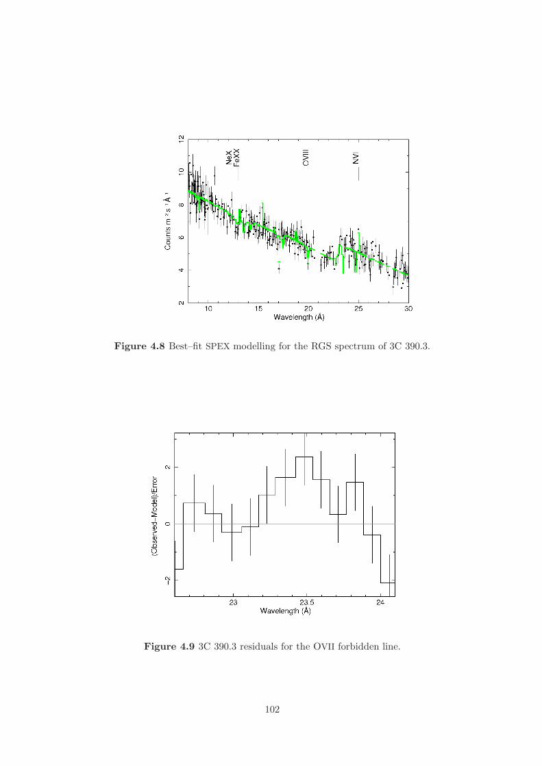
Figure 4.8 Best–fit SPEX modelling for the RGS spectrum of 3C 390.3.
Figure 4.9 3C 390.3 residuals for the OVII forbidden line.
102
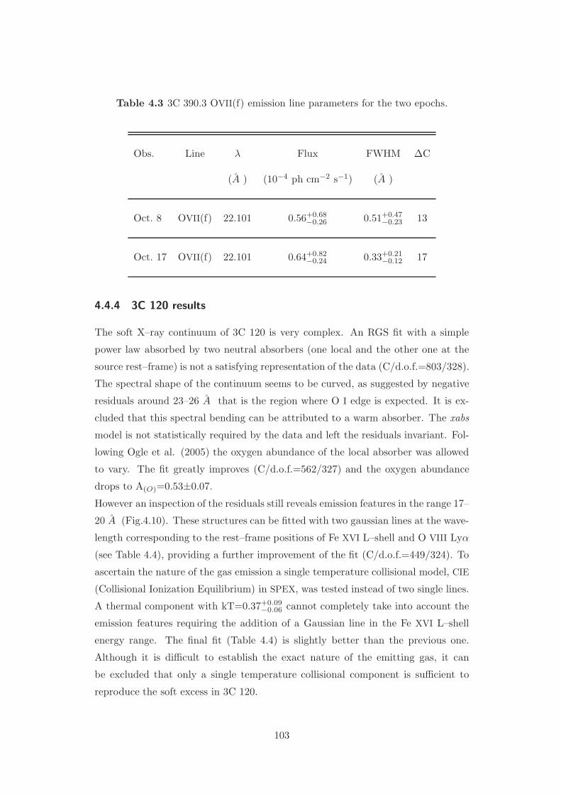
Table 4.3 3C 390.3 OVII(f) emission line parameters for the two epochs.
Obs. Line λ Flux FWHM ∆C
(A ) (10−4 ph cm−2 s−1) (A )
Oct. 8 OVII(f) 22.101 0.56+0.68−0.26 0.51+0.47
−0.23 13
Oct. 17 OVII(f) 22.101 0.64+0.82−0.24 0.33+0.21
−0.12 17
4.4.4 3C 120 results
The soft X–ray continuum of 3C 120 is very complex. An RGS fit with a simple
power law absorbed by two neutral absorbers (one local and the other one at the
source rest–frame) is not a satisfying representation of the data (C/d.o.f.=803/328).
The spectral shape of the continuum seems to be curved, as suggested by negative
residuals around 23–26 A that is the region where O I edge is expected. It is ex-
cluded that this spectral bending can be attributed to a warm absorber. The xabs
model is not statistically required by the data and left the residuals invariant. Fol-
lowing Ogle et al. (2005) the oxygen abundance of the local absorber was allowed
to vary. The fit greatly improves (C/d.o.f.=562/327) and the oxygen abundance
drops to A(O)=0.53±0.07.
However an inspection of the residuals still reveals emission features in the range 17–
20 A (Fig.4.10). These structures can be fitted with two gaussian lines at the wave-
length corresponding to the rest–frame positions of Fe XVI L–shell and O VIII Lyα
(see Table 4.4), providing a further improvement of the fit (C/d.o.f.=449/324). To
ascertain the nature of the gas emission a single temperature collisional model, CIE
(Collisional Ionization Equilibrium) in SPEX, was tested instead of two single lines.
A thermal component with kT=0.37+0.09−0.06 cannot completely take into account the
emission features requiring the addition of a Gaussian line in the Fe XVI L–shell
energy range. The final fit (Table 4.4) is slightly better than the previous one.
Although it is difficult to establish the exact nature of the emitting gas, it can
be excluded that only a single temperature collisional component is sufficient to
reproduce the soft excess in 3C 120.
103
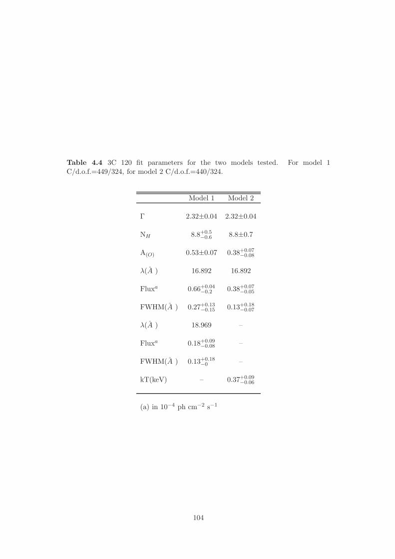
Table 4.4 3C 120 fit parameters for the two models tested. For model 1C/d.o.f.=449/324, for model 2 C/d.o.f.=440/324.
Model 1 Model 2
Γ 2.32±0.04 2.32±0.04
NH 8.8+0.5−0.6 8.8±0.7
A(O) 0.53±0.07 0.38+0.07−0.08
λ(A ) 16.892 16.892
Fluxa 0.66+0.04−0.2 0.38+0.07
−0.05
FWHM(A ) 0.27+0.13−0.15 0.13+0.18
−0.07
λ(A ) 18.969 –
Fluxa 0.18+0.09−0.08 –
FWHM(A ) 0.13+0.18−0 –
kT(keV) – 0.37+0.09−0.06
(a) in 10−4 ph cm−2 s−1
104
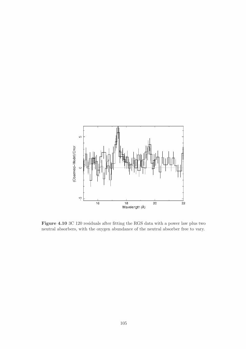
Figure 4.10 3C 120 residuals after fitting the RGS data with a power law plus twoneutral absorbers, with the oxygen abundance of the neutral absorber free to vary.
105

106
5A small sample of Broad Line
Radio Galaxies
High–resolution data were collected from literature in an effort to build a sample
of BLRGs sources. It consists of four sources: 3C 390.3, 3C 120, 3C 382 and
3C 445. 3C 445 is included because Reeves et al. (2010) claimed the Chandra/LETG
detection of an outflowing and clumpy accretion disk wind, in addition to the soft
X–ray emission lines.
Although small in size, the sample can help in characterizing the physical properties
of the absorbing gas in AGNs able to produce powerful relativistic outflow.
The main properties of each object are reported in Table 5.1, where the redshift,
the jet inclination angles, the black hole masses, the ionizing luminosities between
1—1000 Ry, and the radio luminosity at 151 MHz in units of W Hz−1 sr−1 are
listed.
5.1 Warm Absorber Physical Properties
In Table 5.2 the column density, the ionization parameter, the outflow velocity, the
mimimum and maximum radii of the WA are reported for each source of the sample.
In order to establish the location of the emitting/absorbing region, the BLR and
the torus distances are also listed (see Section 4.5 for the description of how the
distances are estimated).
As expected, the absorption lines due to photoionization and photoexcitation
107
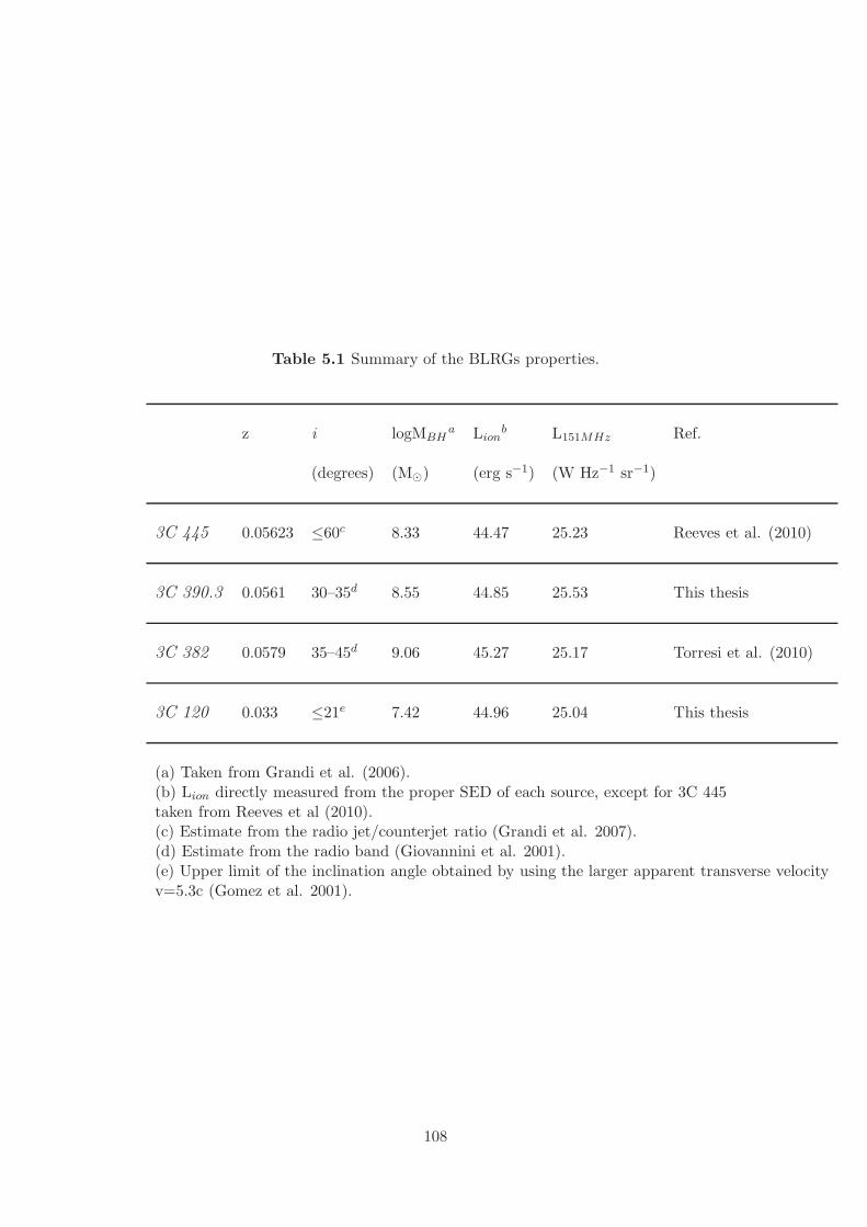
Table 5.1 Summary of the BLRGs properties.
z i logMBHa Lion
b L151MHz Ref.
(degrees) (M⊙) (erg s−1) (W Hz−1 sr−1)
3C 445 0.05623 ≤60c 8.33 44.47 25.23 Reeves et al. (2010)
3C 390.3 0.0561 30–35d 8.55 44.85 25.53 This thesis
3C 382 0.0579 35–45d 9.06 45.27 25.17 Torresi et al. (2010)
3C 120 0.033 ≤21e 7.42 44.96 25.04 This thesis
(a) Taken from Grandi et al. (2006).(b) Lion directly measured from the proper SED of each source, except for 3C 445taken from Reeves et al (2010).(c) Estimate from the radio jet/counterjet ratio (Grandi et al. 2007).(d) Estimate from the radio band (Giovannini et al. 2001).(e) Upper limit of the inclination angle obtained by using the larger apparent transverse velocityv=5.3c (Gomez et al. 2001).
108
processes are preferentially observed in RGs seen at small inclination angles (i.e.,
3C 382 and 3C 390.3). On the contrary, the emission lines, produced by the inverse
processes, are dominant in 3C 445 (Grandi et al. 2007; Reeves et al. 2010), the
only source with the jet pointed away from the observer. Note that no WA could
be detected in 3C 120, the BLRG in the sample with the smallest inclination angle
(i<21) and the only one with a γ–ray counterpart discovered by Fermi (see Section
1.3.1). Despite of the small sample of available objects, there is evidence that the
physical conditions and location of the warm gas are not always the same. The
deduced high velocity (vout∼104 km s−1), high column density (NH>1023 cm−2)
and low ionization parameter logξ=1.4 erg cm s−1 of the wind in 3C 445 indicate
a probable origin in the disk (Reeves et al. 2010). On the contrary, the ionization
parameters of 3C 382 and 3C 390.3 are higher, the outflows are slower and probably
nearby the torus, far from the central engine. It is worth noting that the outflows
have been detected with different instruments. In particular, the fast wind has
been discovered analyzing the hard part of the spectrum (E>6 keV) with very long
LETG exposure (200 ks). The high energy features are elusive and are not always
detected. For example, a so strong edge at 7 keV in the spectrum of 3C 445 was not
successively observed by Suzaku (Braito et al. 2011). The occasional occurrence of
these events could explain the difficulty in catching them. Conversely, the presence
of slow outflows in the soft X–ray band (E<2 keV) is well ascertained. This seems to
suggest that, a different perspective of the same WA phenomenon can be obtained
looking at different regions of the spectrum with different instruments. Hints of the
multi–phase nature of the WA was also provided by the RGS analysis of 3C 390.3,
where an indication of a dual absorber was found in the longer observation. This
further suggests that the availability of high–resolution spectra with a high S/N
ratio is mandatory to explore the complexity of the gas.
5.2 Warm Absorber Energetics in BLRGs
Table 5.3 reports the inflow and outflow mass rate (Macc, Mout), the kinetic lu-
minosity of the outflow (Eout) and of the jet (Pjet), and the accretion luminosity
that we assume Lbol=Lacc=ηMc2. The mass accretion rate Macc was calculated for
η=0.1.
The mass outflow rate estimates how much mass is carried out through the wind,
and can be expressed as:
109

Table 5.2 For each source the warm absorber parameters, i.e., logNH1 , logξ, vout,together with the estimated minimum (rmin) and maximum (rmax) distance of theWA in pc, the distance of the BLR (rBLR) and of the torus (rtorus) from the centralengine, respectively, are reported.
log NH log ξ vout rmin rmax rBLR rtorus
(cm−2) (erg cm s−1) (km s−1) pc pc pc pc
3C 445 23.3 1.4 104 0.01 - 0.02 0.45
3C 390.3 20.7 2.08 <600 ≥9 ≤450 0.02 0.7
3C 382 22.5 2.69 1000 ≥10 ≤60 0.06 1.5
3C 120 - - - - - 0.03 0.8
110
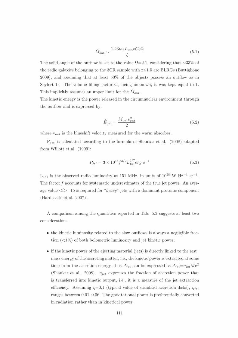
Mout ∼1.23mpLionvCvΩ
ξ(5.1)
The solid angle of the outflow is set to the value Ω=2.1, considering that ∼33% of
the radio galaxies belonging to the 3CR sample with z≤1.5 are BLRGs (Buttiglione
2009), and assuming that at least 50% of the objects possess an outflow as in
Seyfert 1s. The volume filling factor Cv being unknown, it was kept equal to 1.
This implicitly assumes an upper limit for the Mout.
The kinetic energy is the power released in the circumnuclear environment through
the outflow and is expressed by:
Eout =Moutv
2out
2(5.2)
where vout is the blueshift velocity measured for the warm absorber.
Pjet is calculated according to the formula of Shankar et al. (2008) adapted
from Willott et al. (1999):
Pjet = 3 × 1045f3/2L6/7151erg s−1 (5.3)
L151 is the observed radio luminosity at 151 MHz, in units of 1028 W Hz−1 sr−1.
The factor f accounts for systematic underestimates of the true jet power. An aver-
age value <f>=15 is required for “heavy” jets with a dominant protonic component
(Hardcastle et al. 2007) .
A comparison among the quantities reported in Tab. 5.3 suggests at least two
considerations:
• the kinetic luminosity related to the slow outflows is always a negligible frac-
tion (<1%) of both bolometric luminosity and jet kinetic power;
• if the kinetic power of the ejecting material (jets) is directly linked to the rest–
mass energy of the accreting matter, i.e., the kinetic power is extracted at some
time from the accretion energy, thus Pjet can be expressed as Pjet=ηjetMc2
(Shankar et al. 2008). ηjet expresses the fraction of accretion power that
is transferred into kinetic output, i.e., it is a measure of the jet extraction
efficiency. Assuming η=0.1 (typical value of standard accretion disks), ηjet
ranges between 0.01–0.06. The gravitational power is preferentially converted
in radiation rather than in kinetical power.
111
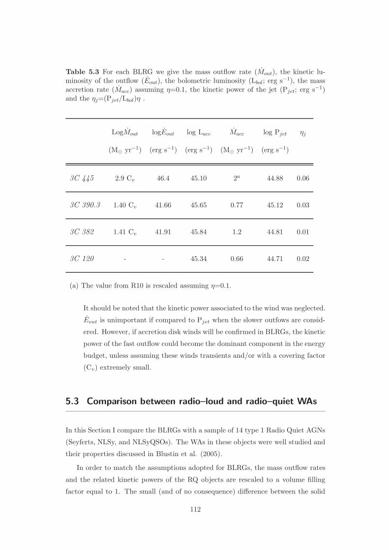
Table 5.3 For each BLRG we give the mass outflow rate (Mout), the kinetic lu-minosity of the outflow (Eout), the bolometric luminosity (Lbol; erg s−1), the massaccretion rate (Macc) assuming η=0.1, the kinetic power of the jet (Pjet; erg s−1)and the ηj=(Pjet/Lbol)η .
LogMout logEout log Lacc Macc log Pjet ηj
(M⊙ yr−1) (erg s−1) (erg s−1) (M⊙ yr−1) (erg s−1)
3C 445 2.9 Cv 46.4 45.10 2a 44.88 0.06
3C 390.3 1.40 Cv 41.66 45.65 0.77 45.12 0.03
3C 382 1.41 Cv 41.91 45.84 1.2 44.81 0.01
3C 120 - - 45.34 0.66 44.71 0.02
(a) The value from R10 is rescaled assuming η=0.1.
It should be noted that the kinetic power associated to the wind was neglected.
Eout is unimportant if compared to Pjet when the slower outfows are consid-
ered. However, if accretion disk winds will be confirmed in BLRGs, the kinetic
power of the fast outflow could become the dominant component in the energy
budget, unless assuming these winds transients and/or with a covering factor
(Cv) extremely small.
5.3 Comparison between radio–loud and radio–quiet WAs
In this Section I compare the BLRGs with a sample of 14 type 1 Radio Quiet AGNs
(Seyferts, NLSy, and NLSyQSOs). The WAs in these objects were well studied and
their properties discussed in Blustin et al. (2005).
In order to match the assumptions adopted for BLRGs, the mass outflow rates
and the related kinetic powers of the RQ objects are rescaled to a volume filling
factor equal to 1. The small (and of no consequence) difference between the solid
112
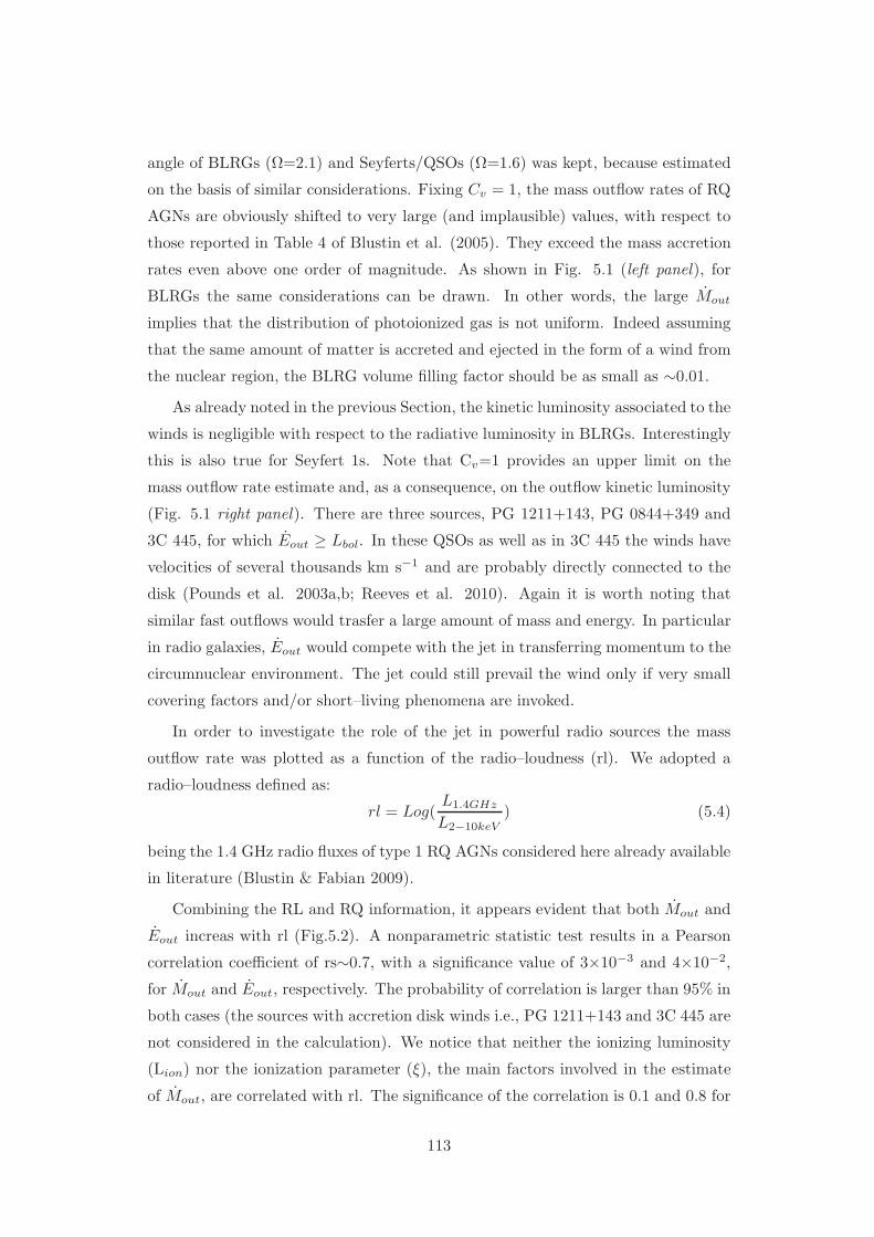
angle of BLRGs (Ω=2.1) and Seyferts/QSOs (Ω=1.6) was kept, because estimated
on the basis of similar considerations. Fixing Cv = 1, the mass outflow rates of RQ
AGNs are obviously shifted to very large (and implausible) values, with respect to
those reported in Table 4 of Blustin et al. (2005). They exceed the mass accretion
rates even above one order of magnitude. As shown in Fig. 5.1 (left panel), for
BLRGs the same considerations can be drawn. In other words, the large Mout
implies that the distribution of photoionized gas is not uniform. Indeed assuming
that the same amount of matter is accreted and ejected in the form of a wind from
the nuclear region, the BLRG volume filling factor should be as small as ∼0.01.
As already noted in the previous Section, the kinetic luminosity associated to the
winds is negligible with respect to the radiative luminosity in BLRGs. Interestingly
this is also true for Seyfert 1s. Note that Cv=1 provides an upper limit on the
mass outflow rate estimate and, as a consequence, on the outflow kinetic luminosity
(Fig. 5.1 right panel). There are three sources, PG 1211+143, PG 0844+349 and
3C 445, for which Eout ≥ Lbol. In these QSOs as well as in 3C 445 the winds have
velocities of several thousands km s−1 and are probably directly connected to the
disk (Pounds et al. 2003a,b; Reeves et al. 2010). Again it is worth noting that
similar fast outflows would trasfer a large amount of mass and energy. In particular
in radio galaxies, Eout would compete with the jet in transferring momentum to the
circumnuclear environment. The jet could still prevail the wind only if very small
covering factors and/or short–living phenomena are invoked.
In order to investigate the role of the jet in powerful radio sources the mass
outflow rate was plotted as a function of the radio–loudness (rl). We adopted a
radio–loudness defined as:
rl = Log(L1.4GHz
L2−10keV) (5.4)
being the 1.4 GHz radio fluxes of type 1 RQ AGNs considered here already available
in literature (Blustin & Fabian 2009).
Combining the RL and RQ information, it appears evident that both Mout and
Eout increas with rl (Fig.5.2). A nonparametric statistic test results in a Pearson
correlation coefficient of rs∼0.7, with a significance value of 3×10⁻³ and 4×10⁻²,
for Mout and Eout, respectively. The probability of correlation is larger than 95% in
both cases (the sources with accretion disk winds i.e., PG 1211+143 and 3C 445 are
not considered in the calculation). We notice that neither the ionizing luminosity
(Lion) nor the ionization parameter (ξ), the main factors involved in the estimate
of Mout, are correlated with rl. The significance of the correlation is 0.1 and 0.8 for
113
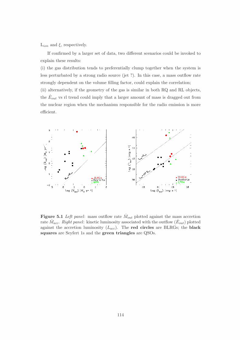
Lion and ξ, respectively.
If confirmed by a larger set of data, two different scenarios could be invoked to
explain these results:
(i) the gas distribution tends to preferentially clump together when the system is
less perturbated by a strong radio source (jet ?). In this case, a mass outflow rate
strongly dependent on the volume filling factor, could explain the correlation;
(ii) alternatively, if the geometry of the gas is similar in both RQ and RL objects,
the Eout vs rl trend could imply that a larger amount of mass is dragged out from
the nuclear region when the mechanism responsible for the radio emission is more
efficient.
Figure 5.1 Left panel : mass outflow rate Mout plotted against the mass accretionrate Macc. Right panel : kinetic luminosity associated with the outflow (Eout) plottedagainst the accretion luminosity (Lacc). The red circles are BLRGs; the blacksquares are Seyfert 1s and the green triangles are QSOs.
114
Figure 5.2 Left panel : mass outflow rate Mout plotted against the radio loudness(rl=L1.4GHz/L2−10keV ). Right panel : kinetic luminosity associated with the outflow(Eout) plotted against rl. The red circles are BLRGs; the black squares areSeyfert 1s and the green triangles are QSOs.
115

116

6Discussion and Conclusions
One of the main debated astrophysical problem is the role of AGN feedback in
the formation and evolution of galaxies. According to popular AGN/galaxy co–
evolutionary scenarios, once central supermassive black holes reach masses >107–
108 M⊙, the AGN can heat the ISM inhibiting accretion and star formation.
AGN/environment interaction can be split in two broad categories: the radiative
mode, including ionization, heating, and radiation pressure (e.g. Ciotti &Ostriker
2007) and the mechanical mode via winds and jets (e.g. Ciotti, Ostriker, &Proga
2009; Shin, Ostriker, & Ciotti 2010).
This thesis presents a study of the circumnuclear environment of powerful radio
galaxies (3C 33, 3C 382, 3C 390.3 and 3C 120), drawing some observational conclu-
sions on the interplay among the nuclear engine and the surrounding medium. The
investigation is based on high–resolution spectroscopy, a relatively new technique
that offers the unique possibility to explore in detail the gaseous environment of
AGNs. Unlike RQ AGNs, the application of this technique on RL sources has just
started.
The detection of emission lines, very similar to those observed in Seyfert 2s, in
the soft X–ray spectrum of the obscured BLRG 3C 445 (Grandi et al. 2007) opened
a new window of investigation. The soft excess could be explained as emission
from photoionized gas rather than jet radiation (as proposed by other authors),
suggesting that in RL AGNs radiative mechanisms are at work also on kpc scales.
This thesis provides further and new evidences of the presence of warm gas in
RL AGNs, showing that slow outflowing gas can survive in environments where
relativistic collimated plasma (jet) propagates.
117

In particular:
• The analysis of all the data of 3C 33, available in the XMM–Newton and
Chandra archives, allowed the detection of soft emission lines, similar to those
observed in Seyfert 2 galaxies (Guainazzi & Bianchi 2007). Moreover it was
shown that this gas is positioned in the NLR, as attested by the perfect over-
lapping between the Chandra soft X–ray contours and the [OIII]λ5007 image
(Fig.3.8).
• Unambiguously signatures of warm gas were observed, for the first time, in
two BLRGs, namely 3C 382 and 3C 390.3. The XMM-Newton/RGS spectra
revealed the presence of a gas (logξ=2.08–2.69), outflowing at velocities around
102−3 km s−1, probably located in the NLR (Chapter 4).
These results show that, like in Seyfert galaxies (Kinkhabwala et al. 2002), absorp-
tion and emission processes in RL AGNs can occur in the same plasma. Depending
on the line–of–sight, different features can be revealed. Indeed the absorption lines
due to photoionization and photoexcitation processes are preferentially observed in
BLRGs, while the emission lines, produced by the inverse processes, are detected in
sources with wide viewing angles (for example 3C 33). Interesting enough, no WA
is detected in 3C 120, the BLRG with the smallest inclination angle (i<21) and
the only in the sample with a γ–ray counterpart recently discovered by Fermi.
In this thesis it is also shown that:
• The warm gas is probably clumped. Indeed, assuming a volume filling factor
equal to 1, the mass outflow rates are implausible and much higher than the
mass accretion rates. Mout and Macc become comparable when Cv is as small
as 0.01.
• The warm absorber detected in 3C 390.3 and 3C 382 is slow and probably
related to the torus. Therefore, even considering upper limits on the mass
outflow rate (if Cv=1), the kinetic luminosity related to the NLR outflow is
always a negligible fraction (<1%) of both bolometric luminosity and jet ki-
netic power. It is however possible that the location of the ionized outflow is
not unique. Recently it has been proposed that a very fast (vout=104 km s−1)
winds, similar to those detected in the RQ PG 1211+143 and PG 0844+349,
is also present in 3C 445. In these QSOs as well as in 3C 445 the winds have
velocities of several thousands km s−1 and are probably directly connected
118
to the disk (Pounds et al. 2003a,b; Reeves et al. 2010). It should be noted
that similar fast outflows would carry a huge amount of mass and energy.
In particular in radio galaxies, Eout would compete with the jet in transfer-
ring momentum to the circumnuclear environment (unless very small covering
factors and/or transient phenomena are invoked).
Aware of the limited number of BLRGs for which WA information is available, a
first comparison between the RL and RQ properties is proposed in this thesis. The
conclusions are:
• Unlike RL AGNs, Seyfert 1 warm absorbers are typically structured and out-
flowing at velocities ranging from a few to hundreds km s−1 (Blustin et al.
2005). The average number of modelled phases is two, but it seems that bet-
ter quality data would require a larger number of phases. However as pointed
out by Blustin et al. (2005), the number of phases itself is not a fundamental
parameter to understand the ionization structure, but is more likely a function
of the today’s instrumentation and data quality.
• In both RQ and RL objects, the mass outflow rates exceed the mass accretion
rate, as expected if the warm gas distribution is not uniform (i.e., a volume
filling factor ≪ 1).
• The kinetic luminosity related to the slow outflow is always negligible with
respect to the accretion luminosity, independently on the radio power of the
AGN.
• The mass outflow rate and kinetic luminosity seem to increase with the radio
loudness (Fig. 5.2). Brighter radio sources have larger values of mass outflow
rates. Two possible interpretations are suggested here:
i) as the Eout is dependent on Cv, warm gas fills larger volumes in stronger
radio sources, or ii) if the gas distribution is similar in both RL and RQ
objects, the presence of intense radio emission (jets?) favors the escape of a
larger amount of mass in the form of wind.
6.1 Future perspectives
The application of high–resolution spectroscopy on RL AGNs is just begun if com-
pared with the amount of observations and results obtained for RQ AGNs so far.
119

Now we know that the circumnuclear environment of radio galaxies is similar to that
of Seyferts, at least on kpc scales. However there are still many open questions:
- is there any link between accretion and ejection ?
- is there any link between winds and jets ?
- how do the outflows really influence the host galaxy?
- how long do they last? Are they short–living phenomena or not?
- are they really present only in a part of AGNs (50% in Seyfert 1s, 50% (?) in
BLRGs), or could they be ubiquitous but not oriented along out line–of–sight
(Elvis et al. 2000), or with a turbulent velocity or column density too low to
be observed with today’ s instrumentation (Blustin et al. 2005)
The next generation X–ray satellites (IXO and Astro–H) will answer these questions.
As an example, we show the excellent quality spectra of 3C 33 and 3C 382 that will
be obtained with IXO in very short (10 ksec) exposures (Fig. 6.1 and 6.2). This
simple exercise shows the great potentiality of IXO. Its huge sensitivity will permit to
exploit all the spectroscopical diagnostics (see Chapter 2), essentials to understand
the physical, geometrical and kinematic properties of warm absorbers in local radio
galaxies. More important, these measurements will be extended to a very large
sample of radio–loud sources located at different redshifts, allowing to follow how
feedback works in the galaxy evolution.
120
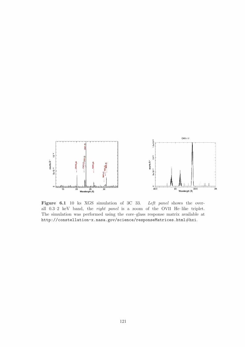
Figure 6.1 10 ks XGS simulation of 3C 33. Left panel shows the over-all 0.3–2 keV band, the right panel is a zoom of the OVII He–like triplet.The simulation was performed using the core–glass response matrix available athttp://constellation-x.nasa.gov/science/responseMatrices.html#hxi.
121
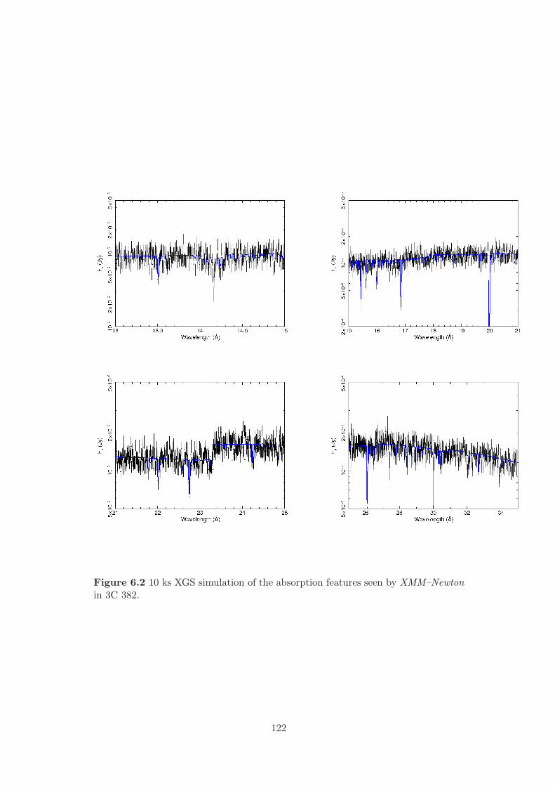
Figure 6.2 10 ks XGS simulation of the absorption features seen by XMM–Newtonin 3C 382.
122
AThe XMM–Newton observatory
A.1 Basic characteristics
The XMM–Newton 1 (X–ray Multi Mirror) observatory (Jansen et al. 2001) was
launched in December 1999 and it is dedicated to the exploration of the X–ray
Universe in the 0.15–15 keV band. Its orbit is highly eccentric (Fig.A.1) between
7000 km (perigee) and 114000 km (apogee) and it has an inclination of about 40
with respect to the ecliptic. The orbital period is of about 48 hours, thus it is possible
to perform uninterrupted observations as long as 150 ks (∼40 hours). Thanks to
the six scientific instruments carried onboard, which work simultaneously, XMM–
Newton allows to explore the X–ray and optical/UV bands at the same time. The
scientific instruments are (Fig.A.2):
1. the EPIC (European Photon Imaging Cameras): three CCD cameras for X–
ray imaging and moderate resolution (E/∆E∼20–50) spectroscopy placed at
the foci of the three X–ray telescopes: two MOS (Metal Oxyde Semiconductor)
cameras (Turner et a. 2001), and one pn camera (Struder et al. 2001).
2. the RGS (Reflection Grating Spectrometers) (den Herder et al. 2001): two
identical spectrometers dedicated to high resolution X–ray spectroscopy, that
are working in the 0.33–2.5 keV (5–38 A) energy band. The two instruments
are made by dispersion gratings placed on the light path of the two MOS
cameras.
1http://xmm.esac.esa.int
123

3. the OM (Optical Monitor) (Mason et al. 2001): optical/UV telescope with
an aperture of ∼30 cm, for imaging and grism spectroscopy.
Figure A.1 Representation of the highly elliptical orbit of the XMM–Newton satel-lite.
Figure A.2 Sketch of the XMM–Newton payload. At the bottom left there are themirror modules, two of which are equipped with Reflection Grating Arrays. At thebottom right there are the focal X–ray instruments, the EPIC MOS and EPIC pn.Obscured by the lower mirror module is the OM.
124
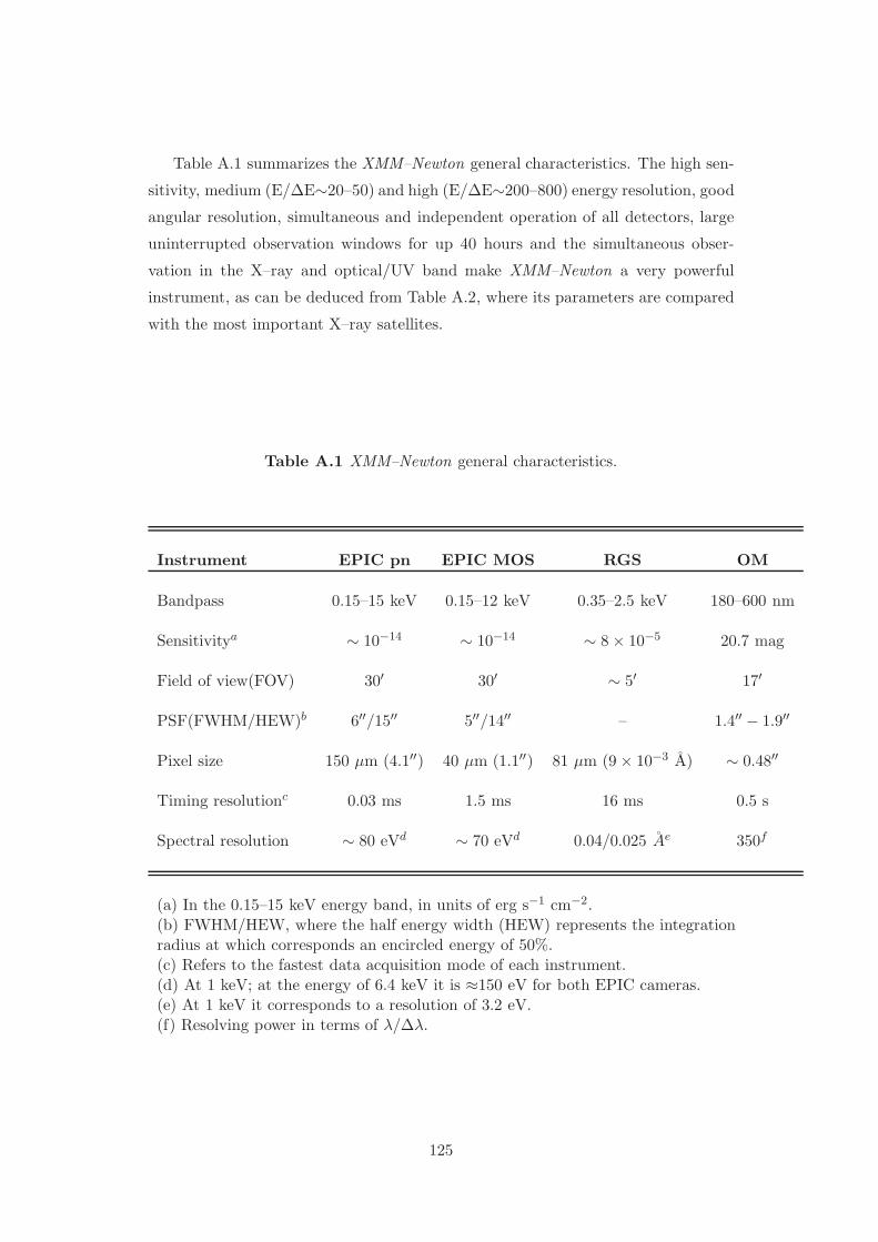
Table A.1 summarizes the XMM–Newton general characteristics. The high sen-
sitivity, medium (E/∆E∼20–50) and high (E/∆E∼200–800) energy resolution, good
angular resolution, simultaneous and independent operation of all detectors, large
uninterrupted observation windows for up 40 hours and the simultaneous obser-
vation in the X–ray and optical/UV band make XMM–Newton a very powerful
instrument, as can be deduced from Table A.2, where its parameters are compared
with the most important X–ray satellites.
Table A.1 XMM–Newton general characteristics.
Instrument EPIC pn EPIC MOS RGS OM
Bandpass 0.15–15 keV 0.15–12 keV 0.35–2.5 keV 180–600 nm
Sensitivitya ∼ 10−14 ∼ 10−14 ∼ 8 × 10⁻⁵ 20.7 mag
Field of view(FOV) 30′ 30′ ∼ 5′ 17′
PSF(FWHM/HEW)b 6′′/15′′ 5′′/14′′ – 1.4′′ − 1.9′′
Pixel size 150 µm (4.1′′) 40 µm (1.1′′) 81 µm (9 × 10⁻³ A) ∼ 0.48′′
Timing resolutionc 0.03 ms 1.5 ms 16 ms 0.5 s
Spectral resolution ∼ 80 eVd ∼ 70 eVd 0.04/0.025 Ae 350f
(a) In the 0.15–15 keV energy band, in units of erg s−1 cm−2.(b) FWHM/HEW, where the half energy width (HEW) represents the integrationradius at which corresponds an encircled energy of 50%.(c) Refers to the fastest data acquisition mode of each instrument.(d) At 1 keV; at the energy of 6.4 keV it is ≈150 eV for both EPIC cameras.(e) At 1 keV it corresponds to a resolution of 3.2 eV.(f) Resolving power in terms of λ/∆λ.
125
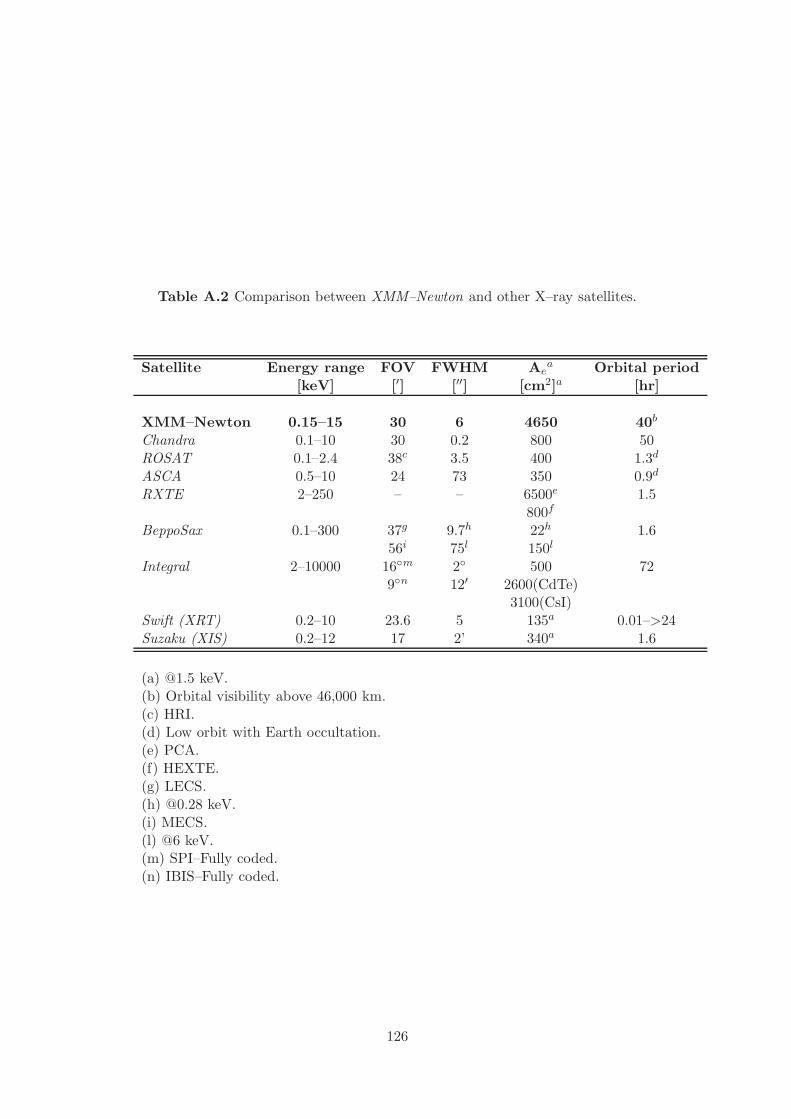
Table A.2 Comparison between XMM–Newton and other X–ray satellites.
Satellite Energy range FOV FWHM Aea Orbital period
[keV] [′] [′′] [cm2]a [hr]
XMM–Newton 0.15–15 30 6 4650 40b
Chandra 0.1–10 30 0.2 800 50ROSAT 0.1–2.4 38c 3.5 400 1.3d
ASCA 0.5–10 24 73 350 0.9d
RXTE 2–250 – – 6500e 1.5800f
BeppoSax 0.1–300 37g 9.7h 22h 1.656i 75l 150l
Integral 2–10000 16m 2 500 729n 12′ 2600(CdTe)
3100(CsI)Swift (XRT) 0.2–10 23.6 5 135a 0.01–>24Suzaku (XIS) 0.2–12 17 2’ 340a 1.6
(a) @1.5 keV.(b) Orbital visibility above 46,000 km.(c) HRI.(d) Low orbit with Earth occultation.(e) PCA.(f) HEXTE.(g) LECS.(h) @0.28 keV.(i) MECS.(l) @6 keV.(m) SPI–Fully coded.(n) IBIS–Fully coded.
126

A.2 The X–ray telescopes
XMM–Newton carries three grazing incidence Wolter type 1 X–ray telescopes (Fig.A.3),
each with 58 concentric mirror shells. At the foci of the three telescopes there are
the EPIC cameras and the RGS instruments (see Section A.4). Co–aligned with
the X–ray telescopes is the OM.
This optical design provides to XMM–Newton the highest effective area of any
X–ray mission so far, that is 4650 cm2 at 1.5 keV and ∼3000 cm2 at 6 keV (see
Table A.2). Fig.A.4 shows the effective area of the individual X–ray instruments
on XMM–Newton. As shown in Section A.3 the effective areas of the two MOS
cameras are lower than that of the pn, because only part of the incoming radiation
(∼44%) falls onto these detectors, while the other part falls onto the RGS as it is
shown in Fig.A.5. An important critical parameter for a detector is its ability in
focussing photons. This parameter is measured through the shape and dimension
of the point spread function (PSF). The PSF describes how the light coming from
a pointlike source is distributed on the detector. The PSF FWHM of the XMM–
Newton telescopes is about 6”. The PSF integrated in two dimensions as a function
of the distance from the central peak, gives the fractional encircled energy, that is
the amount of energy within a certain radius (see Fig.A.6, A.7).
Figure A.3 Optical system of image reflection adopted for X–ray telescopes. Theprimary mirror is a paraboloid, while the secondary mirror is hyperboloid.
127
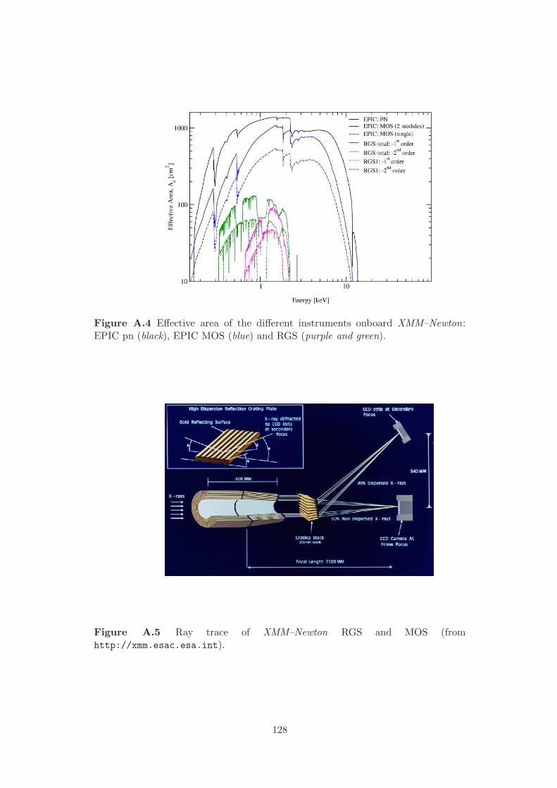
Figure A.4 Effective area of the different instruments onboard XMM–Newton:EPIC pn (black), EPIC MOS (blue) and RGS (purple and green).
Figure A.5 Ray trace of XMM–Newton RGS and MOS (fromhttp://xmm.esac.esa.int).
128
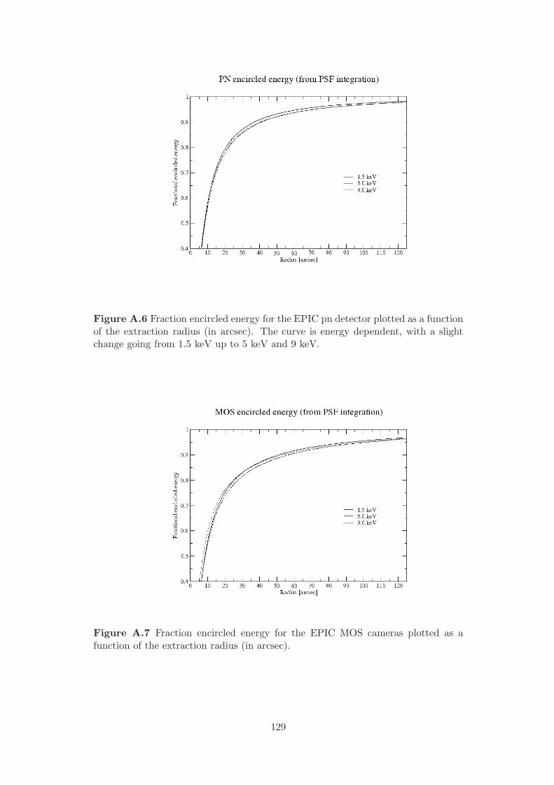
Figure A.6 Fraction encircled energy for the EPIC pn detector plotted as a functionof the extraction radius (in arcsec). The curve is energy dependent, with a slightchange going from 1.5 keV up to 5 keV and 9 keV.
Figure A.7 Fraction encircled energy for the EPIC MOS cameras plotted as afunction of the extraction radius (in arcsec).
129
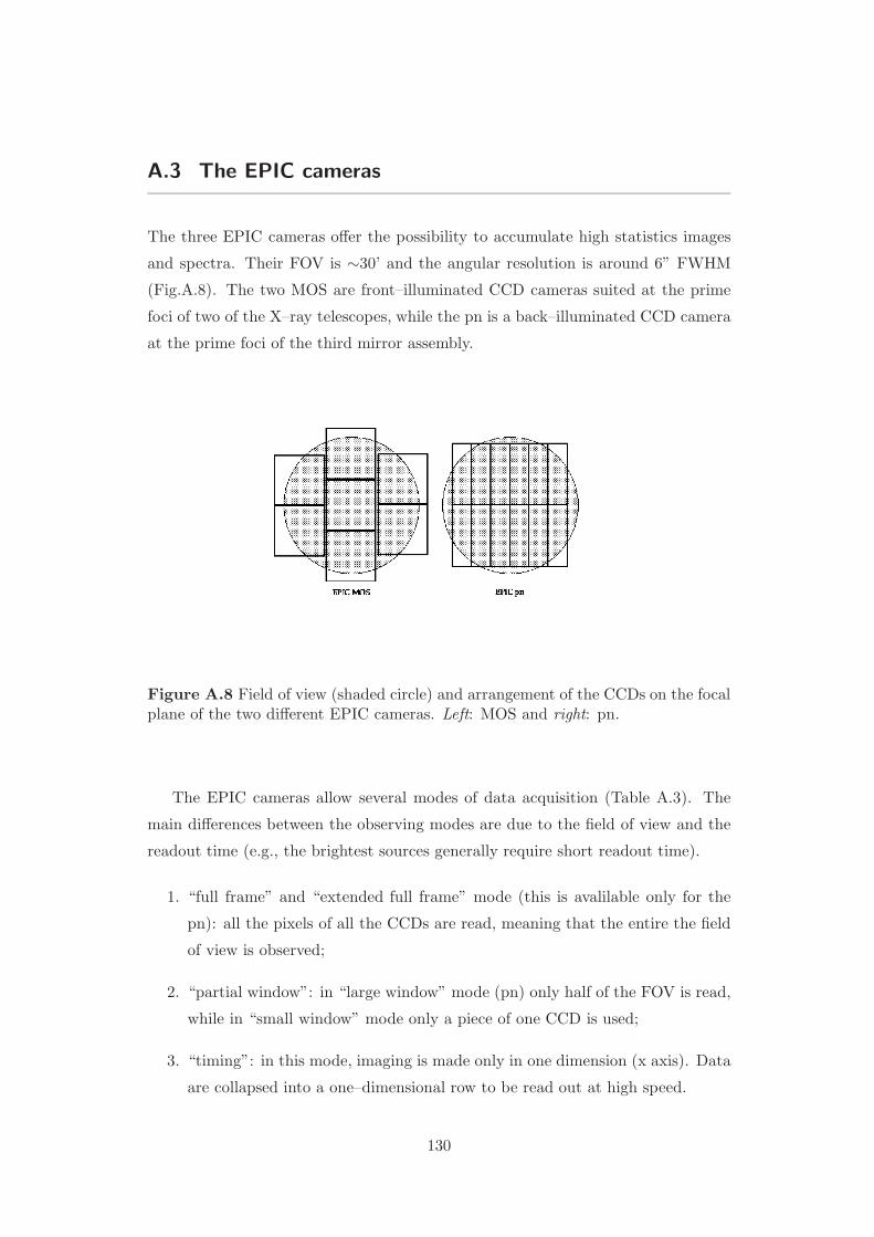
A.3 The EPIC cameras
The three EPIC cameras offer the possibility to accumulate high statistics images
and spectra. Their FOV is ∼30’ and the angular resolution is around 6” FWHM
(Fig.A.8). The two MOS are front–illuminated CCD cameras suited at the prime
foci of two of the X–ray telescopes, while the pn is a back–illuminated CCD camera
at the prime foci of the third mirror assembly.
Figure A.8 Field of view (shaded circle) and arrangement of the CCDs on the focalplane of the two different EPIC cameras. Left: MOS and right: pn.
The EPIC cameras allow several modes of data acquisition (Table A.3). The
main differences between the observing modes are due to the field of view and the
readout time (e.g., the brightest sources generally require short readout time).
1. “full frame” and “extended full frame” mode (this is avalilable only for the
pn): all the pixels of all the CCDs are read, meaning that the entire the field
of view is observed;
2. “partial window”: in “large window” mode (pn) only half of the FOV is read,
while in “small window” mode only a piece of one CCD is used;
3. “timing”: in this mode, imaging is made only in one dimension (x axis). Data
are collapsed into a one–dimensional row to be read out at high speed.
130

Table A.3 Field of view and time resolution for different observing modes of theEPIC pn and EPIC MOS cameras.
EPIC pn FOV Temporal resolution(1 pixel=4.1′′) (pixel) (ms)
Full frame 376 × 384 73.4Extended full frame 376 × 384 200Large window 198 × 384 48Small window 63 × 64 6Timinga 64 × 200 0.03Burstb 64 × 20 0.007
EPIC MOS FOV Temporal resolution(1 pixel=1.1′′) (pixel) (s)
Full frame 600 × 600 2.6Large window 300 × 300 0.9Small window 100 × 100 0.3Timinga 100 × 600 1.5 × 10⁻³
(a) In this mode the read–out cycle of the chips is reducedbecause the events detected on diffrentpixels are integrated along only one spatial coordinate.(b) A special flavour of the timing mode of the EPIC pn camerawhich offers very high time resolution, but has a very lowduty cycle of 3%.
131
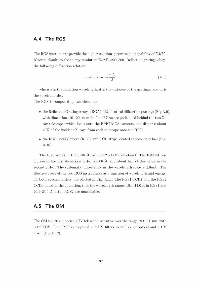
A.4 The RGS
The RGS instruments provide the high–resolution spectroscopic capability of XMM–
Newton, thanks to the energy resolution E/∆E∼200–800. Reflection gratings obeys
the following diffraction relation:
cosβ = cosα +mλ
δ(A.1)
where λ is the radiation wavelength, d is the distance of the gratings, and m is
the spectral order.
The RGS is composed by two elements:
• the Reflection Grating Arrays (RGA): 182 identical diffraction gratings (Fig.A.9),
with dimensions 10×20 cm each. The RGAs are positioned behind the two X–
ray telescopes which focus onto the EPIC MOS cameras, and disperse about
40% of the incident X–rays from each telescope onto the RFC;
• the RGS Focal Camera (RFC): two CCD strips located at secondary foci (Fig.
A.10).
The RGS works in the 5–38 A (or 0.33–2.5 keV) waveband. The FWHM res-
olution in the first dispersion order is 0.06 A, and about half of this value in the
second order. The systematic uncertainty in the wavelength scale is ±8mA. The
effective areas of the two RGS instruments as a function of wavelength and energy,
for both spectral orders, are plotted in Fig. A.11. The RGS1 CCD7 and the RGS2
CCD4 failed in the operation, thus the wavelength ranges 10.4–14.0 A in RGS1 and
20.1–23.9 A in the RGS2 are unavailable.
A.5 The OM
The OM is a 30 cm optical/UV telescope, sensitive over the range 180–600 nm, with
∼17’ FOV. The OM has 7 optical and UV filters as well as an optical and a UV
grism (Fig.A.12).
132
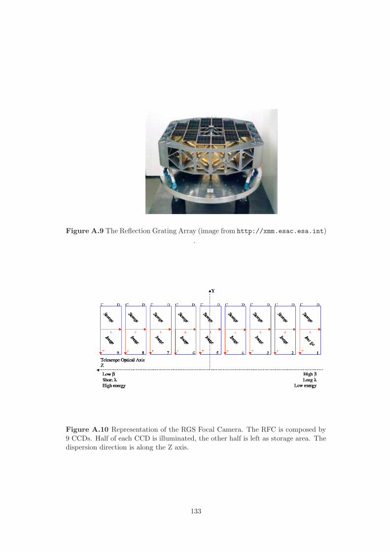
Figure A.9 The Reflection Grating Array (image from http://xmm.esac.esa.int)
.
Figure A.10 Representation of the RGS Focal Camera. The RFC is composed by9 CCDs. Half of each CCD is illuminated, the other half is left as storage area. Thedispersion direction is along the Z axis.
133
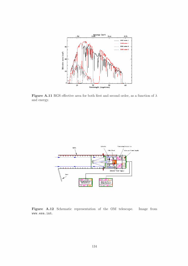
Figure A.11 RGS effective area for both first and second order, as a function of λand energy.
Figure A.12 Schematic representation of the OM telescope. Image fromwww.esa.int.
134

BThe Chandra X–ray observatory
The Chandra X–ray observatory 1 (Fig. B.1), the second satellite capable of high–
resolution X–ray spectroscopy, was launched on July 1999.
Figure B.1 Schematic representation and description of the Chandra satellite. Fig-ure from http://chandra.harvard.edu/resources/illustrations/.
It has a single focusing telescope based on a Wolter type 1 grazing incidence
X–ray mirrors pairs (the High Resolution Mirror Array or HRMA). The mirrors are
combined with 4 science instruments: two focal plane instruments, ACIS and HRC,
and two grating spectrometers, HETG and LETG 2. Unlike XMM–Newton they do
not work simultaneously.
1http://cxc.harvard.edu2http://chandra.harvard.edu/about/science instruments.html
135
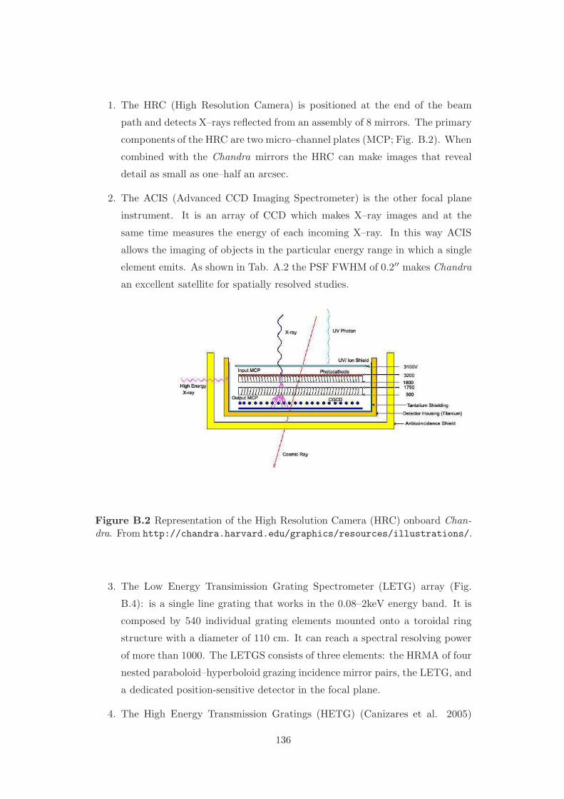
1. The HRC (High Resolution Camera) is positioned at the end of the beam
path and detects X–rays reflected from an assembly of 8 mirrors. The primary
components of the HRC are two micro–channel plates (MCP; Fig. B.2). When
combined with the Chandra mirrors the HRC can make images that reveal
detail as small as one–half an arcsec.
2. The ACIS (Advanced CCD Imaging Spectrometer) is the other focal plane
instrument. It is an array of CCD which makes X–ray images and at the
same time measures the energy of each incoming X–ray. In this way ACIS
allows the imaging of objects in the particular energy range in which a single
element emits. As shown in Tab. A.2 the PSF FWHM of 0.2′′ makes Chandra
an excellent satellite for spatially resolved studies.
Figure B.2 Representation of the High Resolution Camera (HRC) onboard Chan-dra. From http://chandra.harvard.edu/graphics/resources/illustrations/.
3. The Low Energy Transimission Grating Spectrometer (LETG) array (Fig.
B.4): is a single line grating that works in the 0.08–2keV energy band. It is
composed by 540 individual grating elements mounted onto a toroidal ring
structure with a diameter of 110 cm. It can reach a spectral resolving power
of more than 1000. The LETGS consists of three elements: the HRMA of four
nested paraboloid–hyperboloid grazing incidence mirror pairs, the LETG, and
a dedicated position-sensitive detector in the focal plane.
4. The High Energy Transmission Gratings (HETG) (Canizares et al. 2005)
136
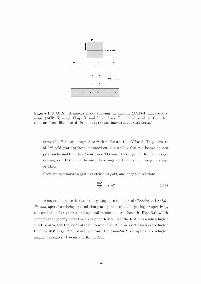
Figure B.3 ACIS instruments layout showing the imaging (ACIS–I) and spectro-scopic (ACIS–S) array. Chips S1 and S3 are back–illuminated, while all the otherchips are front–illuminated. From http://cxc.harvard.edu/cal/Acis/.
array (Fig.B.5): are designed to work in the 0.4–10 keV band. They consists
of 336 gold gratings facets mounted on an assembly that can be swung into
position behind the Chandra mirrors. The inner two rings are the high–energy
grating, or HEG, while the outer two rings are the medium–energy grating,
or MEG.
Both are transmission gratings etched in gold, and obey the relation:
mλ
d= sinθ (B.1)
The major differences between the grating spectrometers of Chandra and XMM–
Newton, apart from being transmission gratings and reflection gratings, respectively,
concerns the effective area and spectral resolution. As shown in Fig. B.6, which
compares the gratings effective areas of both satellites, the RGS has a much higher
effective area, but the spectral resolutions of the Chandra spectrometers are higher
than the RGS (Fig. B.7), basically because the Chandra X–ray optics have a higher
angular resolution (Paerels and Kahn, 2003).
137
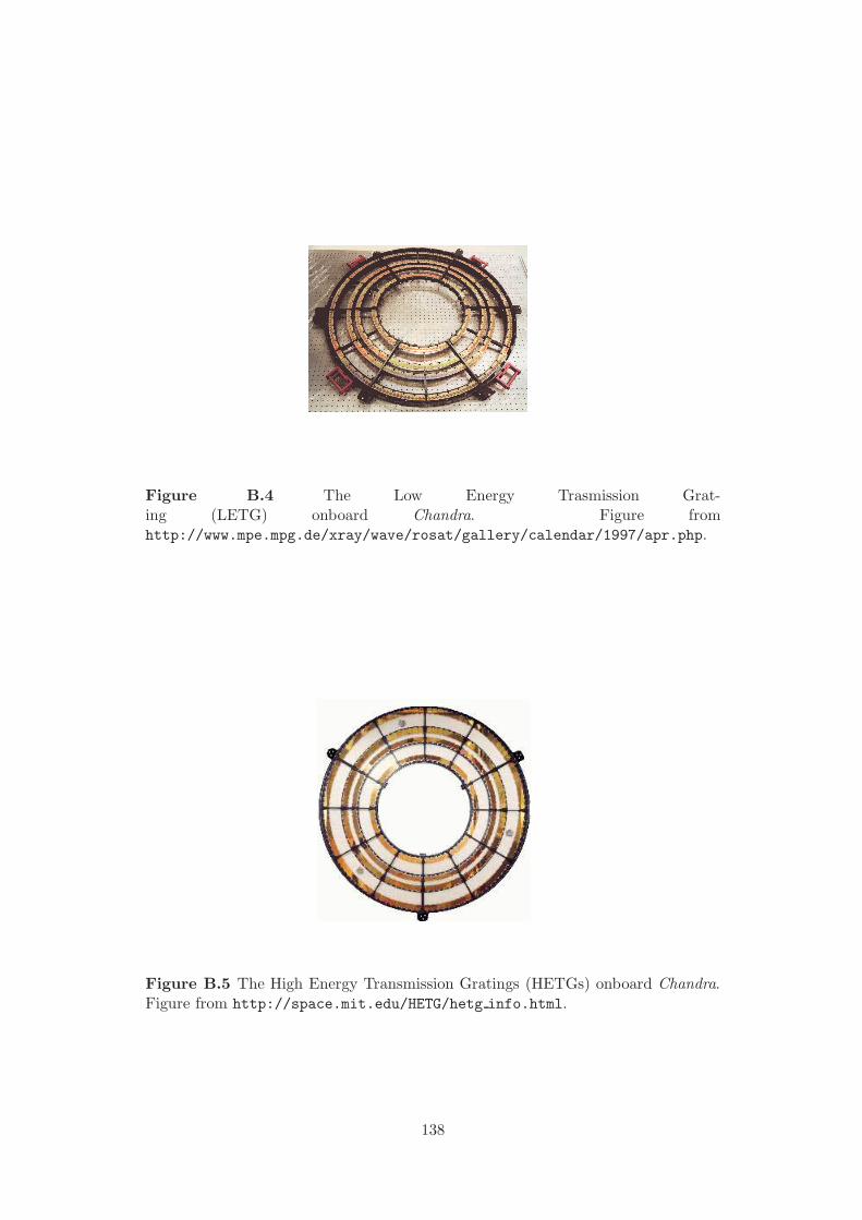
Figure B.4 The Low Energy Trasmission Grat-ing (LETG) onboard Chandra. Figure fromhttp://www.mpe.mpg.de/xray/wave/rosat/gallery/calendar/1997/apr.php.
Figure B.5 The High Energy Transmission Gratings (HETGs) onboard Chandra.Figure from http://space.mit.edu/HETG/hetg info.html.
138
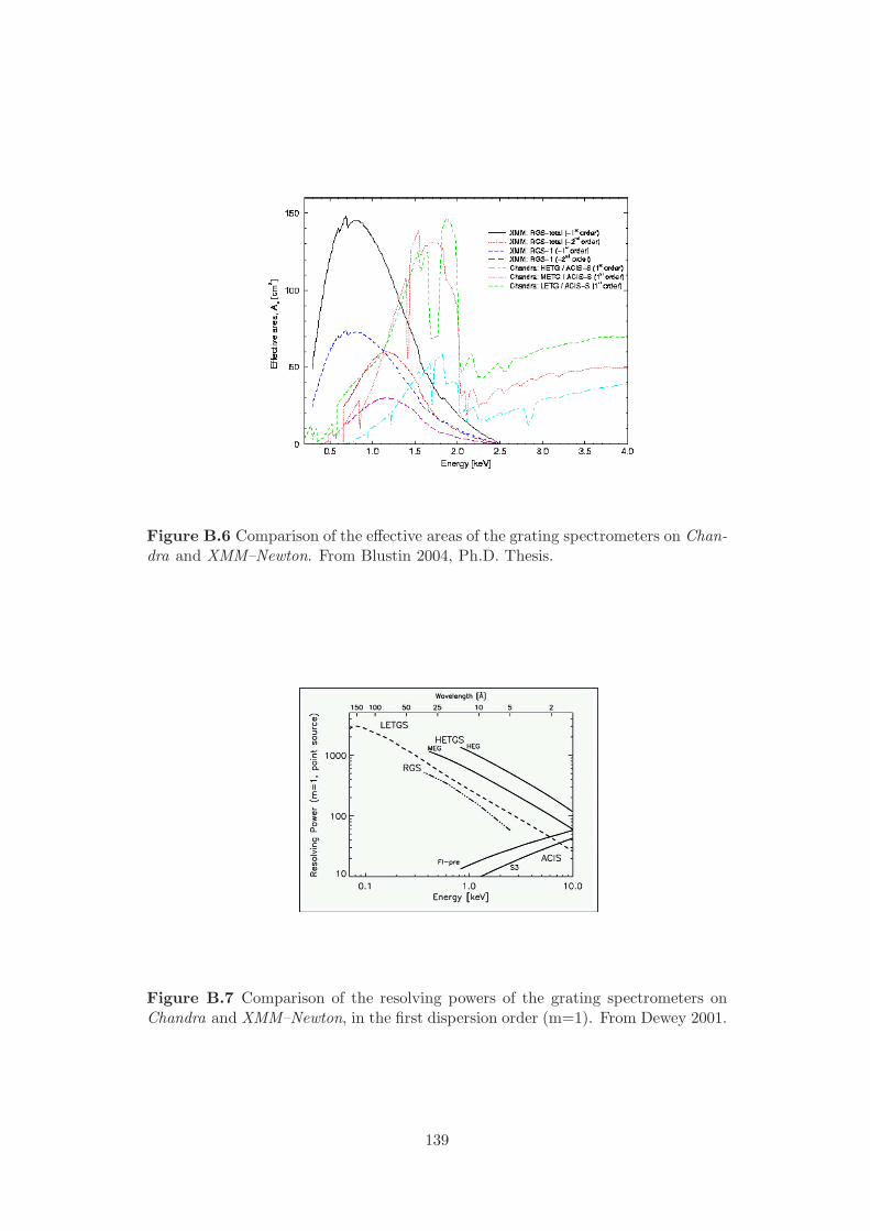
Figure B.6 Comparison of the effective areas of the grating spectrometers on Chan-dra and XMM–Newton. From Blustin 2004, Ph.D. Thesis.
Figure B.7 Comparison of the resolving powers of the grating spectrometers onChandra and XMM–Newton, in the first dispersion order (m=1). From Dewey 2001.
139

140

CThe IXO satellite
The International X–ray Observatory/IXO 1, 2 (Fig. C.1) is a joint effort of NASA,
ESA and JAXA. Its launch is programmed for 2021.
Figure C.1 The IXO satellite.
IXO will incorporate a single large X–ray mirror assembly (3 m2 collecting area
and 5′′ angular resolution) and an extendible optical bench with a focal length of
20 m and a suite of focal plane instruments (Fig. C.2):
1http://sci.esa.int/science-e/www/object/index.cfm?fobjectid=422712http://ixo.gsfc.nasa.gov/
141

- the X–ray Microcalorimeter Spectrometer (XMS), provides high–spectral res-
olution, non–dispersive imaging spectroscopy over the energy range 0.3–7 keV;
- the Wield Field Imager (WFI), is an imaging X–ray spectrometer with a large
FOV (18’ × 18’) and provides images and spectra in the 0.1–15 keV energy
band. The Hard X–ray imager (HXI), mounted directly behind the WFI in
the same instrument extends the energy coverage to 40 keV, working simul-
taneously with the WFI;
- the X–ray grating spectrometer (XGS) is a wavelength–dispersive spectrome-
ter that will provide high spectral resolution in the 0.3–1 keV band. The XGS
will have a spectral resolving power of λ/∆λ=3000 and effective area larger
than 1000 cm2 across its operating band (Fig. C.3). The high–resolution
spectrosocpy is achieved through an array of wavelength–dispersive diffrac-
tion gratings with a fine pitch of 5000 lines/mm or more.
- the High Timing Resolution Spectrometer (HTRS) will perform high preci-
sion timing measurements of brigth X–ray sources. It can observe sources
with fluxes 106 cts/s in the 0.3–10 keV energy band without performance
degradation, and provides moderate spectral resolution of 150 eV FWHM at
6 keV.
- the X–ray Polarimeter (XPOL) is an imaging polarimeter with polarization
sensitivity of 1% for a source with F2−10keV = 1 mCrab in 105 sec of exposure.
Figure C.2 IXO instrument module. Credit: NASA.
142
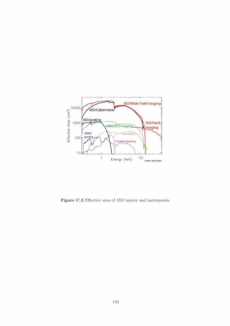
Figure C.3 Effective area of IXO mirror and instruments.
143

144

Acknowledgements
I am sincerely grateful to my supervisor Paola Grandi for the continuous support,
enthusiasm, brilliant and insightful suggestions, and for the significant effort she has
put in this project. I am also indebted to her for always encouraging me to do my
best.
I would like to thank Prof. Giorgio Palumbo for his enthusiastic guidance, he is a
reference of scientific passion and professionality.
A special thank to Matteo Guainazzi for giving me the opportunity to work a few
months at ESAC (among many difficulties!). It was really a pleasure to collaborate
with him.
I am grateful to all the collaborators I have worked with during these three years,
I have learned a lot from fruitful interactions with them.
A big thank goes to my office–mates Valentina for being above all a good friend,
and Barbara for keeping the atmosphere light and providing me lots of chocolate
bars during the writing up of my thesis.
Thanks to all the people working at the IASF institute in Bologna, past and present,
for providing a very friendly and enjoyable atmosphere. In particular thanks to Adri-
ano, Matteo and Enrico for technical assistance whenever my computer crashed, and
to Elisabetta, Pietro, Lorenzo and Giulia. Thanks to my “Spanish” friend Enrica
for the wonderful time spent in Madrid, and to Cristina for being the perfect flat-
mate.
Thanks to Filippo for the many entertaining discussions drinking a glass of good
wine.
Special big big thanks to Chiara, Monica, Lucia, Michela, Francesca, Letizia, Sara,
Maura, Antonella, Marta for being the best friends one could ever have.
Thanks from the deepest of my heart to my parents Sergio and Lorella, my sister
Veronica and the other half of my sky Vito for their love and regardless support.
145

146

Part I
Bibliography
147

Abdo, A.A., et al. 2010a, ApJS, 188, 405
Abdo, A.A., et al. 2010b, ApJ, 715, 429
Abdo, A.A., et al. 2010c, ApJ, 720, 912
Abdo, A.A., et al. 2010d, Science, 328, 725
Abramowicz, M.A., Chen, X., Kato, S., Lasota, J.-P., Regev, O. 1995, ApJ, 438, 37
Aharonian, F. et al. 2003, A&A, 403, L1
Aharonian, F. et al. 2009, ApJ, 695, L40
Alef, W., Wu, S. Y., Preuss, E., Kellermann, K. I., Qiu, Y. H. 1996, A&A, 308, 376
Anders, E., Grevesse, N. 1989, GeCoA, 53, 197
Antonucci, R.R.J., Miller J.S., 1985, ApJ, 297, 621
Antonucci, R.R.J., 1993, ARA&A, 31, 473
Antonucci, R.R.J., Hurt T., Kinney A., 1994, Nature, 371, 313
Antonucci, R.R.J. 2011, arXiv:1101.0837v1
Arnaud, K. A. 1996, XSPEC: the first ten years, in Astronomical Data Analysis
Software and Systems V, ed. G. H. Jacoby, & J. Barnes, ASP Conf. Ser., 101, 17
Atwood, W. B., et al. 2009, ApJ, 697, 1071
Ballantyne, D.R., Fabian, A.C., Iwasawa, K. 2004, MNRAS, 354, 839
Ballantyne, D.R. 2005, MNRAS, 362, 1183 Balmaverde, B., Capetti, A., Grandi,
P. 2006, A&A, 451, 35
Baum, S.A., Heckman, T. 1989, ApJ, 336, 680
Baum, S.A. 1992, Clusters and Superclusters of Galaxies, ed. A.C. Fabian
(Cambridge:CUP), p.171
Baum, S.A., Heckman, T.M., Van Breugel, W. 1992, ApJ, 389, 208
Bautista, M.A., & Kallman, T.R. 2001, ApJS, 134, 139
Behar, E., Sako, M., Kahn, S.M. 2001, ApJ, 563, 497
Belsole, E., Worrall, D.M., Hardcastle, M.J. 2006, MNRAS, 366, 339
Bennett, A.S. 1962, MNRAS, 125, 75
Bianchi, S., Miniutti, G., Fabian, A.C., et al. 2005, MNRAS, 360, 380
Bianchi, S., Guainazzi, M., & Chiaberge, M. 2006, A&A, 448, 499
Black, A.R.S., Baum, S.A., Leahy, J.P., Perley, R.A., Riley, J.M., Scheuer, P.A.G.
1992, MNRAS, 256, 186
Blandford, R.D., & Begelman, M. 1999, MNRAS, 303, L1
Blustin, A. J., Branduardi-Raymont, G., Behar, E., et al., 2002, A&A, 392, 453
Blustin, A.J. 2004, Ph.D. Thesis, AA (MSSL–UCL)
Blustin A. J., Page M. J., Fuerst S. V., Branduardi-Raymont G., Ashton C. E.,
2005, A&A, 431, 111
149
Blustin, A.J., Fabian, A.C. 2009, MNRAS, 396, 1732
Bohlin, R.C., Savage, B.D., & Drake, J.F. 1978, ApJ, 224, 132
Braito, V., Reeves, J.N., Sambruna, R.M., Gofford, J. 2011, MNRAS,
arXiv1102.5234
Brinkman, A.C., Kaastra, J.S., van der Meer, R.L.J., Kinkhabwala, A., Behar, E.,
Kahn, S.M., Paerels, F.B.S., Sako, M. 2002, A&A, 396, 761
Burbidge, E.M., 1967, ApJ, 149, L51
Burgess, A.M., Hunstead, R. W. 2006a, AJ, 131, 100
Burgess, A.M., Hunstead, R. W. 2006b, AJ, 131, 114
Buttiglione, S., Capetti, A., Celotti, A., Axon, D.J., Chiaberge, M., et al. 2009,
A&A, 495, 1033
Canizares et al. 2005, PASP, 117, 1144
Cardelli, J.A., Klayton, G.C., Mathis, J.S., 1989, ApJ, 345, 254
Cash W., 1979, ApJ, 228, 939
Chiaberge, M., Capetti, A. & Celotti, A. 2000, A&A 355, 873
Chiaberge, M., Macchetto, F.D., Sparks, W.B. et al. 2002, ApJ, 571, 247
Ciotti, L., Ostriker, J.P. 2007, ApJ, 665, 1038
Ciotti, L., Ostriker, J.P., Proga, D. 2009, ApJ, 699, 89
Cleary, K., Lawrence, C.R., Marshall, J.A., Hao, L., Meier, D. 2007, ApJ, 660, 117
Costantini, E., Kaastra, J.S., Arav, N., Kriss, G.A., Steenbrugge, K.C., et al.
2007, A&A, 461, 121
Crenshaw, D.M., Kraemer, S.B., George, I.M. 2003, ARA&A, 41, 117
den Herder J.W., Brinkmann A.C., Kahn S.M., Branduardi–Raymont G., et al.,
2001, A&A, 365, 7
Dere, et al. 1997, AASS, 125, 149
Donato, D., Sambruna, R.M., & Gliozzi, M. 2004, ApJ, 617, 915
Eracleous, M., & Halpern, J. P. 1998, ApJ, 505, 577
Eracleous, M., Sambruna, R.M., Mushotzky, R.F. 2000, ApJ, 537, 654
Evans, D.A., Hardcastle, M.J., Croston, J.H., Worrall, D.M., Birkinshaw, M. 2005,
MNRAS, 359, 363
Evans, D.A., Worrall, D.M., Hardcastle, M.J., Kraft, R.P., Birkinshaw, M. 2006,
ApJ, 642, 96
Evans, D. A., Reeves, J. N., Hardcastle, M. J., Kraft, R. P., Lee, J. C., Virani, S.
N. 2010, ApJ, 710, 859
Fabbiano, G., Miller, L., Trinchieri, G., Longair, M., Elvis, M. 1984, ApJ, 277, 115
Fanaroff, B. L., Riley, J. M. 1974, MNRAS, 167, 31
150
Ferland, G.J., Korista, K.T., Verner, D.A., Ferguson, J.W., Kingdon, J.B., &
Verner, E.M. 1998, PASP, 110, 761
Ferrarese, L., Merritt, D. 2000, ApJ, 539, L9
Floyd, D.J.E., Kukula, M.J., Dunlop, J.S., McLure, R.J., Miller, L., Percival,
W.J., Baum, S.A., O’Dea, C.P. 2004, MNRAS, 355, 196
Friedman, H., Lichtman, S.W., Byram, E.T. 1951, Phys. Rev., 83, 1025
Gabriel A.H., Jordan C., 1969, MNRAS, 145, 241
Gallimore, J.F., Baum, S.A., O’Dea, C.P. 1997, Nature, 388, 852
Gebhardt, K., et al. 2000, ApJ, 539, L13
Ghisellini, G., Haardt, F., & Matt, G. 1994, MNRAS, 267, 743
Ghisellini, G., Celotti, A. 2001, MNRAS, 327, 739
Ghisellini, G., Tavecchio, F., Chiaberge, M. 2005, A&A, 432, 401
Ghisellini, G. & Tavecchio, F. 2008, MNRAS, 387, 1669
Ghosh, K. K., Sondararajaperumal, S. 1991, AJ, 102, 1298
Giacconi, R., Gursky, H., Paolini, F., & Rossi, B.B. 1962, PRL, 9, 439
Gierlinski, M., & Done, C., 2004, MNRAS, 349, 7
Giovannini, G., Feretti, L., Gregorini, L., Parma, P. 1988, A&A, 199, 73
Giovannini, G., Cotton, W. D., Feretti, L., Lara, L., Venturi, T. 2001, ApJ, 552,
508
Giovannini, G., Taylor, G.B., Feretti, L., Cooton, W.D., Lara, L., Venturi, T.
2005, ApJ, 618, 635
Giroletti, M. 2008, ASPC, 386, 176
Gliozzi, M., Sambruna, R.M., Eracleous, M. 2003, ApJ, 584, 176
Gliozzi, M., Sambruna, R. M., Eracleous, M., & Yaqoob, T. 2007, ApJ, 664, 88
Gofford, J., Reeves, J.N., Turner, T.J., Tombesi, F., Braito V., et al. 2011,
MNRAS, arXiv1103.0661
Gomez, J., Marscher, A.P., Alberdi, A., et al. 2001, ApJ, 561, L161
Grandi, P., Guainazzi, M., Haardt, F., Maraschi, L., Massaro, E., Matt, G., Piro,
L., Urry, C. M. 1999, A&A, 343, 33
Grandi, P., Maraschi, L., Urry, C.M., & Matt, G. 2001, ApJ, 556, 35
Grandi, P., Malaguti, G., & Fiocchi, M. 2006, ApJ, 642, 113
Grandi, P., Guainazzi, M., Cappi, M., Ponti, G., 2007, MNRAS, L85
Grevesse, N., & Sauval, A. J. 1998, Space Sci. Rev., 85, 161
Guainazzi M., Bianchi S., 2007, MNRAS, 374, 1290
Haardt, F., Maraschi, L., 1991, ApJ, 380, 51
Haardt, F., Maraschi, L., 1993, ApJ, 413, 507
151
Haardt, F., Maraschi, L., Ghisellini, G., 1994, ApJ, 432, 95
Halpern, J.P. 1984, ApJ, 281, 90
Hardcastle, M.J., Birkinshaw, M., & Worrall, D.M. 1998, MNRAS, 294, 615
Hardcastle M.J., Worrall D.M., 1999, MNRAS, 309, 969H
Hardcastle, M.J., Evans, D.A., Croston, J.H. 2006, MNRAS, 370, 1893
Hardcastle, M.J., Evans, D.A., Croston, J.H., 2007, MNRAS, 376, 1849
Harris, D.E., Mossman, A.E., Walker, R.C. 2004, ApJ, 615, 161
Harris, D.E., & Krawczynski, H. 2006, ARAA, 44, 463
Hartman, R.C., et al. 1999, ApJS, 123, 79
Heckman, T.M. 1980, A&A, 87, 152
Heckman, T.M., Carty, T.J., Bothun, G.D. 1985, ApJ, 288, 122H
Heckman, T.M., Smith E.P., Baum S.A., et al., 1986, ApJ, 311, 526
Hewitt, A., Burbidge, G. 1991, ApJS, 75, 297
Ho, L.C. 2008, ARA&A, 46, 475
Ichimaru, S. 1977, ApJ, 214, 840
Jackson, N., Rawlings, S. 1997, MNRAS, 286, 241
Jaffe, W., Ford, H.C., Ferrarese, L., van den Bosch, F., O’Connell, R.W. 1993,
Nature, 364, 213
Jansen, F., Lumb, D., Altieri, B., Clavel, J., Ehle, M., Erd, C., Gabriel, C.,
Guainazzi, M., et al. 2001, A&A, 365, 1
Kaastra, J.S. 1992, An X–Ray Spectral Code for Optically Thin Plasmas, Internal
SRON–Leiden Report, updated version 2.0
Kaastra, J. S., Mewe, R., Nieuwenhuijzen, H., 1996, in Yamashita, K.,Watanabe,
T., eds, UV and X–Ray Spectroscopy of Astrophysical and Laboratory Plasmas.
Universal Academy Press, Tokyo, p. 411
Kaastra, J.S., Paerels, F.B.S., Durret, F., Schindler, S., Richter, P. 2008, Space
Science Reviews, Volume 134, Issue 1-4, pp. 155-190
Kahn, S.M. 2002, “Soft X–Ray Spectroscopy of Astrophysical Plasmas”, Columbia
University
Kahn, S.M., Behar, E., Kinkhabwala, A., & Savin, D.W. 2002, Royal Society of
London Philosophical Transactions Series A, 360, 1923
Kalberla, P.M.W., Burton, W.B., Hartmann, D., Arnal, E.M., Bajaja, E., Morras,
R., & Poppel, W.G.L. 2005, A&A, 440, 775
Kataoka, J., Stawarz, L. 2005, ApJ, 2005, 622, 797
Kataoka, J., Reeves, J.N., Iwasawa, K., et al. 2007, PASJ, 59, 279
Kellermann, K.I., Sramek, R., Schmidt, M., Shaffer, D.B., Green, R. 1989, AJ, 98,
152
1195
Kewley, L.J., Dopita, M.A., Sutherland, R.S., Heisler, C.A., Trevena, J. 2001,
ApJ, 556, 121
Kinkhabwala, A., Sako, M., Behar, E., Kahn, S.M., Paerels, F., Brinkman, A.C.,
Kaastra, J.S., Gu, M.F., Liedhal, D.A. 2002, ApJ, 575, 732
Kinkhabwala, A., 2003, Ph.D. Thesis, AA (Columbia University)
Kirsch, M. 2006, “EPIC status calibration and data analysis”,
XMM-SOC-CAL-TN-0018, Issue 2.5
Klavel, J., Schulz, B., Altieri, B., Barr, P., et al. 2000, A&A, 357, 839
Klockner, H.-R., Baan, W.A., Garrett, M.A. 2003, Nature, 421, 821
Knapp, G.R., Bies, W.E., Van Gorkom, J.H. 1990, AJ, 99, 476
Komatsu, E., et al. 2009, ApJS, 180, 330
Koski, A.T. 1978, ApJ, 223, 56
Kraft, R.P., Birkinshaw, M., Hardcastle, M.J., Evans, D.A., Croston, J.H.,
Worrall, D.M., Murray, S.S. 2007, ApJ, 659, 1008
Krolik, J.H., & Kriss, G.A. 2001, ApJ, 561, 684
Krongold, Y., Nicastro, F., Elvis, M., et al. 2007, ApJ, 659, 1022
Kruper, J. S., Canizares, C. R., Urry, C. M. 1990, ApJS, 74, 347
Laing, R.A., Riley, J.M., Longair, M.S. 1983, MNRAS, 204, 151
Landi et al. 2006, ApJSS, 162, 261
Leahy, J.P., Perley, R.A. 1991, ApJ, 102, 2
Leighly, K. M., O’Brien, P. T. 1997, ApJ, 481, 15
Liedahl, D.A., Osterehled, A.L., Goldstein, W.H. 1995, ApJL, 438, 115
Liedahl, D.A., & Paerels, F. 1996, ApJL, 468, L33
Lightman A.P., White T.R., 1988, ApJ, 335, 57
Lilly, S.J., Longair, M.S. 1982, MNRAS, 199, 1053
Lister, M. L., Cohen, M. H., Homan, D. C., Kadler, M., Kellermann, K. I.,
Kovalev, Y. Y., Ros, E., Savolainen, T., Zensus, J. A. 2009, AJ, 138, 1874
Magdziarz, P., Zdziarski, A.A. 1995, MNRAS, 273, 837
Magorrian, J., Tremaine, S., Richstone, D., Bender, R., et al. 1998, AJ, 115, 2285
Mahadevan, R., Narayan, R., Krolik, J. 1997, ApJ, 486, 268
Maraschi, L., Chiappetti, L., Falomo, R., et al. 1991, ApJ, 368, 138
Marchesini, D., Celotti, A., Ferrarese, L. 2004, MNRAS, 351, 733
Mariotti, M., et al. 2010, ATel#2916
Martel, A. R., et al. 1999, ApJS, 122, 81
Mason, K.O., Breevedl, A., Much, R. 2001, A&A, 365, L36
153
Mathews, W.G., & Ferland, G.J. 1987, ApJ, 323, 456
McKernan, B., Yaqoob, T., Mushotzki, R.F., Ian, M.G., Turner, T.J. 2003, ApJ,
598, L83
McKernan, B., Yaqoob, T., Reynolds, C.S. 2007, MNRAS, 379, 1359
Mewe, R., Gronenschild, E.H.B.M., van den Oord, G.H.J.1985, A&AS, 62, 157
Mewe, R., Lemen, J.R., van den Oord, G.H.J. 1986, A&AS, 65, 511
Migliori, G., Grandi, P., Palumbo, G.G.C., Brunetti, G., Stanghellini, C. 2007,
ApJ, 668, 203
Migliori, G., Grandi, P., Torresi, E., Dermer, C., Finke, J., Celotti, A., Mukherjee,
R., Errando, M., Gargano, F., Giordano, F., Giroletti, M. 2011, submitted to A&A
Miller, C.J., Robert, C.N., Gomez, P.L., Hopkins, A.M., Bernardi, M. 2003, ApJ,
597, 142
Mukherjee, R., Halpern, J., Mirabal, N., Gotthelf, E. V. 2002, ApJ, 574, 693
Muxlow, T.W.B., Garrington, S.T. 1991, “Beams and Jets in Astrophysics” ,
edited by P.H. Hughes, Cambridge Astrophysics Series, p55
Narayan, R., Yi, I. 1994, ApJ, 428, 13
Narayan, R., Yi, I. 1995, ApJ, 452, 710
Netzer, H. 1996, ApJ, 473, 781
Netzer, H. 2004, ApJ, 604, 551
Nicastro, F., Fiore, F., Perola, G. C., Elvis, M., O’Dea, C.P. 1998, PASP, 110, 493
ODea, C.P. 1998, PASP, 110, 493
Ogle, P.M., Brookings, T., Canizares, C.R., Lee, J.C., Marshall, H.L. 2003, A&A,
402, 849
Ogle, P.M., Davis, S.W., Antonucci, R.R.J., et al. 2005, ApJ, 618, 139
Paerels, F.B.S., & Kahn, S.M. 2003, ARA&A, 41, 291
Pearson, T. J., Readhead, A. C. S. 1988, ApJ, 328, 114
Perley, R. A., Dreher, J. W., Cowan, J. J. 1984, ApJ, 285, 35
Peterson, B. M., 1997, “An Introduction to Active Galactic Nuclei”, Cambridge,
UK: Cambridge Univ. Press
Peterson, B. M., Ferrarese, L., Gilbert, K. M., et al., 2004, ApJ, 613, 682
Popescu, C.C., Hopp, U., Hagen, H.J., Elsaesser, H. 1996, A&AS, 116, 43
Porquet, D., Dubau, J. 2000, A&AS, 143, 495
Porquet D., Mewe, R., Dubau, J., Raassen, A.J.J., Kaastra, J.S. 2001, A&A, 376,
1113
Porquet, D., Dubau, J., Grosso, N. 2010, Space Science Reviews
Pounds, K.A., King, A.R., Page, K.L., O’Brien, P.T. 2003a, MNRAS, 346, 1025
154
Pounds, K.A., Reeves, J.N., King, A.R. 2003b, MNRAS, 345, 705
Pounds, K.A., & Page, K.L. 2005, MNRAS, 360, 1123
Pounds, K.A., & Vaughan, S. 2006, MNRAS, 368, 707
Prestage, R.M., Peacock, J.A. 1988, MNRAS, 230, 131
Prieto, M.A. 2000, MNRAS, 316, 442
Proga, D., & Kallman, T.R. 2004, ApJ, 616, 688
Quillen, A.C., Almog, Jessica, Ukita, Mihoko 2003, AJ, 126, 2677
Ramos Almeida, C., Perez Garcia, A.M., Acosta-Pulido, J.A. and Rodriguez
Espinosa, J.M. 2007, AJ, 134, 2006
Raymond, J.C., Smith, B.W. 1977, ApJS, 35, 419
Rees, M.J . 1984, ARA&A, 22, 471
Reeves, J. N., Sambruna, R.M., Braito, V., Eracleous, M. 2009, ApJ, 702, 187
Reeves, J. N., Gofford, J., Braito, V., Sambruna, R. 2010, ApJ, 725, 803
Reynolds C. S., 1997, MNRAS, 286, 513
Risaliti, G. 2002, A&A, 386, 679
Rybicki, G., Lightman, A.P. 1979, Radiative Processes in Astrophysics, New York,
Wiley–Interscience, 393 pp.
Rudnick, L., Jones, T.W., Fiedler, R. 1986, AJ, 91, 1111
Sako, M., Kahn, S.M., Paerels, F., et al. 2000a, ApJ, 543, L115
Sako, M., Kahn, S.M., Paerels, F., Liedahl, D.A. 2000b, ApJ, 542, 648 Sako, M.,
Kahn, S.M., Behar, E., Kaastra, J.S., Brinkman, A.C., Boller, T., et al. 2001,
A&A, 365, L168
Salpeter, E.E., 1964, ApJ, 140, 796
Sambruna R.M., Eracleous M., Mushotzky R.F. 1999, ApJ, 526, 60
Sambruna, R.M., Netzer, H., Kaspi, S., et al. 2001, ApJ, 546L, 13S
Sambruna R.M., Reeves J.N., Braito V., 2007, ApJ, 665, 1030
Sambruna, R. M., Reeves, J. N., Braito, V., Lewis, K. T., Eracleous, M., et al.
2009, ApJ, 700, 1473
Sanders, D. B., Phinney, E. S., Neugebauer, G., Soifer, B. T., Matthews, K. 1989,
ApJ, 347, 29
Santos–Lleo, M., Schartel, N., Tananbaum, H., Tucker, W., Weisskopf, M.C. 2010,
arXiv1003.1961
Scheuer, P.A.G., Readhead, A.C.S. 1979, Nature, 277, 182
Seielstad, G.A., Cohen, M.H., Linfield, R.P., et al. 1979, ApJ, 229, 53
Shakura N. I., Sunyaev R., 1973, A&A, 24, 337
Shankar, F., Cavaliere, A., Cirasuolo, M., & Maraschi, L. 2008, ApJ, 676, 131
155
Shin, M.–S.; Ostriker, J.P., Ciotti, L. 2010, ApJ, arXiv1003.1108
Shull, J.M., Van Steenberg, M.E. 1985, ApJ, 294, 599
Smith, R.K., Brickhouse, N.S., Liedahl, D.A.; Raymond, J.C. 2001, ApJ, 556, 91
Spergel, D.N., et al. 2007, ApJS, 170, 377
Spinrad, H., Marr, J., Aguilar, L., Djorgovski, S. 1985, PASP, 97, 932
Struder, L., Briel, U., Dennerl, K., et al., 2001, A&A, 365, 18
Tadhunter, C.N., Morganti, R., Robinson, A., Dickson, R., Villar-Martin, M.,
Fosbury, R.A.E. 1998, MNRAS, 298, 1035
Tadhunter, C. 2008, New Astronomy Reviews, 52, 227
Tarter, C., Tucker, W.H., and Salpeter, E. 1969, ApJ, 156, 943
Terashima, Y., & Wilson, A.S. 2003, ApJ, 583, 145
Torresi, E., Grandi, P., Guainazzi, M., Palumbo, G.G.C., Ponti, G., Bianchi, S.
2009, A&A, 498, 61
Torresi, E., Grandi, P., Longinotti, A. L., Guainazzi, M., Palumbo, G. G. C.,
Tombesi, F., Nucita, A. 2010, MNRAS, 401L, 10
Tremaine, S., et al. 2002, ApJ, 574, 740
Turner, A.K., Fabian, A.C., Lee, J.C., Vaughan, S. 2004, MNRAS, 353, 319
Turner, M.J.L., Abbey, A., Arnaud, M., Balasini, M., Barbera, M., Belsole, E.,
Bennie, P. J., Bernard, J. P., Bignami, G.F., et al. 2001, A&A, 365, 27
Urry M.C., Padovani P., 1995, PASP, 107, 803
Walker, R.C., Benson, J.M., Unwin, S.C. 1987, ApJ, 316, 546
Wamsteker, W., Wang, T.-G., Schartel, N., Vio, R. 1997, MNRAS, 288, 225
Willott, C.J., Rawlings, S., Blundell, K.M., & Lacy, M. 1999, MNRAS, 309, 1017
Wilson, A.S., Young, A.J., Shopbell, P.L. 2001, ASP Conference Series, Vol. 250,
editors R.A. Laing & K.M. Blundell
Wu, W., Clayton, G.C.; Gordon, K.D., Misselt, K.A., Smith, T.L., Calzetti, D.
2002, ApJS, 143, 377
Yee, H.K.C., Oke, J.B. 1981, ApJ, 248, 472
Yaqoob, T., McKernan, B., Kraemer, S.B., et al. 2003, ApJ, 582, 105
Yaqoob, T, Padmanabhan, U. 2004, ApJ, 604, 63
Zeldovich, Ya.B. 1964, Soviet Physics – Doklady, 9, 195
Zdziarski, A.A., Grandi, P. 2001, ApJ, 551, 18
Zheng, W. 1996, AJ, 111, 1498
156

Publications
The following list reports the papers related to this thesis and written from the
work made during the three years of Ph.D. They correspond to part of chapters1,
3 and 4 of this thesis.
1. “3C 33: another case of photoionized soft X–ray emission in radio galaxies”;
Torresi, E., Grandi, P., Guainazzi, M., Palumbo, G.G.C., Ponti, G., Bianchi,
S. 2009, A&A, 498, 61
2. “First high–resolution detection of a warm absorber in the Broad Line Radio
Galaxy 3C 382”; Torresi, E., Grandi, P., Longinotti, A.L., Guainazzi, M.,
Palumbo, G.G.C., Tombesi, F., Nucita, A. 2010, MNRAS Letters, 401, 10
3. “Warm Absorber energetics in Broad Line Radio Galaxies”; Torresi, E.,
Grandi, P., Costantini, E., Palumbo, G.G.C. 2011, submitted to MNRAS
4. “Fermi Large Area Telescope observations of Misaligned AGN ”; Abdo et al.
2010, ApJ, 720, 912: Contact authors: P. Grandi, G. Malaguti, G. Tosti, C.
Monte
5. “Implications for the jet structure from multiwavelength observations of NGC 6251”;
Migliori, G., Grandi, P., Torresi, E., Dermer, C., Finke, J., Celotti, A.,
Mukherjee, R., Errando, M., Gargano, F., Giordano, F., Giroletti, M. 2011,
submitted to A&A
157