the gamess-uk tutorial session 1 introduction and program ... · lcsc’2004 tutorial, 18 october...
TRANSCRIPT

LCSC’2004 Tutorial, 18 October 2004 1
CSE Computational Science & Engineering Department
The GAMESS-UK Tutorial
Session 1
Introduction and Program Basics
Martyn F. Guest and Jens M.H.Thomas
CCLRC Daresbury Laboratory
http://www.cfs.dl.ac.uk/tutorials/gamess-uk_LCSC.1.pdf
LCSC’2004 Tutorial, 18 October 2004 2
CSE Computational Science & Engineering Department
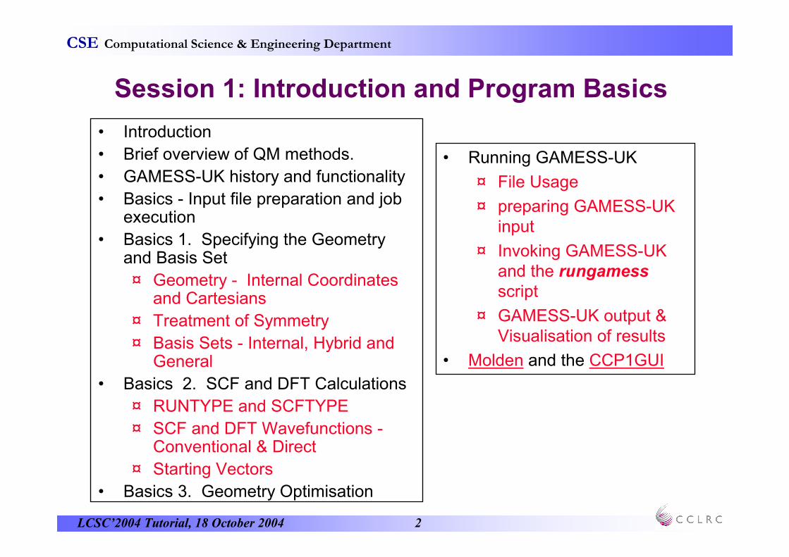
Session 1: Introduction and Program Basics
• Introduction
• Brief overview of QM methods.
• GAMESS-UK history and functionality
• Basics - Input file preparation and job execution
• Basics 1. Specifying the Geometry and Basis Set
¤ Geometry - Internal Coordinates and Cartesians
¤ Treatment of Symmetry
¤ Basis Sets - Internal, Hybrid and General
• Basics 2. SCF and DFT Calculations
¤ RUNTYPE and SCFTYPE
¤ SCF and DFT Wavefunctions -Conventional & Direct
¤ Starting Vectors
• Basics 3. Geometry Optimisation
• Running GAMESS-UK
¤ File Usage
¤ preparing GAMESS-UK input
¤ Invoking GAMESS-UK and the rungamessscript
¤ GAMESS-UK output & Visualisation of results
• Molden and the CCP1GUI
LCSC’2004 Tutorial, 18 October 2004 3
CSE Computational Science & Engineering Department
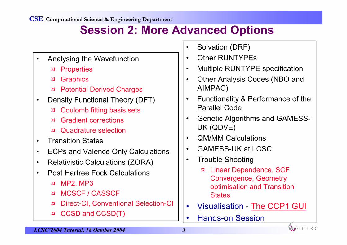
Session 2: More Advanced Options
• Analysing the Wavefunction
¤ Properties
¤ Graphics
¤ Potential Derived Charges
• Density Functional Theory (DFT)
¤ Coulomb fitting basis sets
¤ Gradient corrections
¤ Quadrature selection
• Transition States
• ECPs and Valence Only Calculations
• Relativistic Calculations (ZORA)
• Post Hartree Fock Calculations
¤ MP2, MP3
¤ MCSCF / CASSCF
¤ Direct-CI, Conventional Selection-CI
¤ CCSD and CCSD(T)
• Solvation (DRF)
• Other RUNTYPEs
• Multiple RUNTYPE specification
• Other Analysis Codes (NBO and AIMPAC)
• Functionality & Performance of the Parallel Code
• Genetic Algorithms and GAMESS-UK (QDVE)
• QM/MM Calculations
• GAMESS-UK at LCSC
• Trouble Shooting
¤ Linear Dependence, SCF Convergence, Geometry optimisation and Transition States
• Visualisation - The CCP1 GUI
• Hands-on Session

LCSC’2004 Tutorial, 18 October 2004 4
CSE Computational Science & Engineering Department
Overview of QM methods

LCSC’2004 Tutorial, 18 October 2004 5
CSE Computational Science & Engineering Department
Hartree Fock Calculations 1.
• The Self-consistent field (SCF) process
¤ Initial guess of the wavefunction
¤ iterative solution - self consistency
• Open Shell calculations
¤ UHF
• Different orbitals for alphaand beta spin electrons
• Solve alpha and beta secular equations
¤ ROHF
• Same orbitals for different spin,
• but different occupations (more alpha electrons than beta)
¤ GVB (Generalised Valence Bond)
• Doubly occupied & singly occupied orbitals, bonding / anti-bonding pairs
MOAOPµµµµνννν
dgemm
Integrals
VXC
VCoul
V1e
Sequential
Eigensolver
Fρρρρσσσσ
guess
orbitals
If Converged

LCSC’2004 Tutorial, 18 October 2004 6
CSE Computational Science & Engineering Department
• Conventional SCF
¤ Store 2-electron integrals on file
¤ Efficiency improved by neglecting small integrals
• Direct SCF
¤ Compute integrals whenever needed
¤ Efficiency improved by pre-screening (taking into account)
¤ ∆-density matrix
• Direct vs. Conventional
¤ Conventional:
• requires less computation
¤ Direct:
• requires much less disk space
• allows for dynamic load balancing and avoids I/O bottleneck on parallel machines
Hartree Fock Calculations 2.
jjCC τσ

LCSC’2004 Tutorial, 18 October 2004 7
CSE Computational Science & Engineering Department
Derivatives
• First derivative provides atomic forces
¤ geometry optimisation and transition state searches to locate stationary points on potential energy surfaces (PEs)
• Second derivatives
¤ vibrational frequencies and infrared intensities
¤ analytic form implemented for HF, MP2 and DFT
¤ characterisation of stationary points
• (minima, transition states etc.)
• Other derivatives
¤ polarisabilities
¤ magnetisability
¤ Raman intensitiesAmos, R. D., 1987, in Adv. Chem. Phys., pp 99

LCSC’2004 Tutorial, 18 October 2004 8
CSE Computational Science & Engineering Department
Analysing the Wavefunction
• A variety of one-electron properties
¤ dipole moment
¤ electrostatic potentials
¤ electric field
¤ electric field gradient
¤ quadrupole moment
¤ octupole moment
¤ hexadecapole moments
¤ spin densities
• Population analysis(atomic charges, bond and orbital analysis)
• Generate localised molecular orbitals (LMOs)
• graphical analysis (electron density, orbital amplitude, electrostatic potential maps)
• distributed multipoleanalysis (DMA)
• Morokuma energy decomposition analysis
From the converged From the converged wavefunctionwavefunction we can compute:we can compute:
LCSC’2004 Tutorial, 18 October 2004 9
CSE Computational Science & Engineering Department
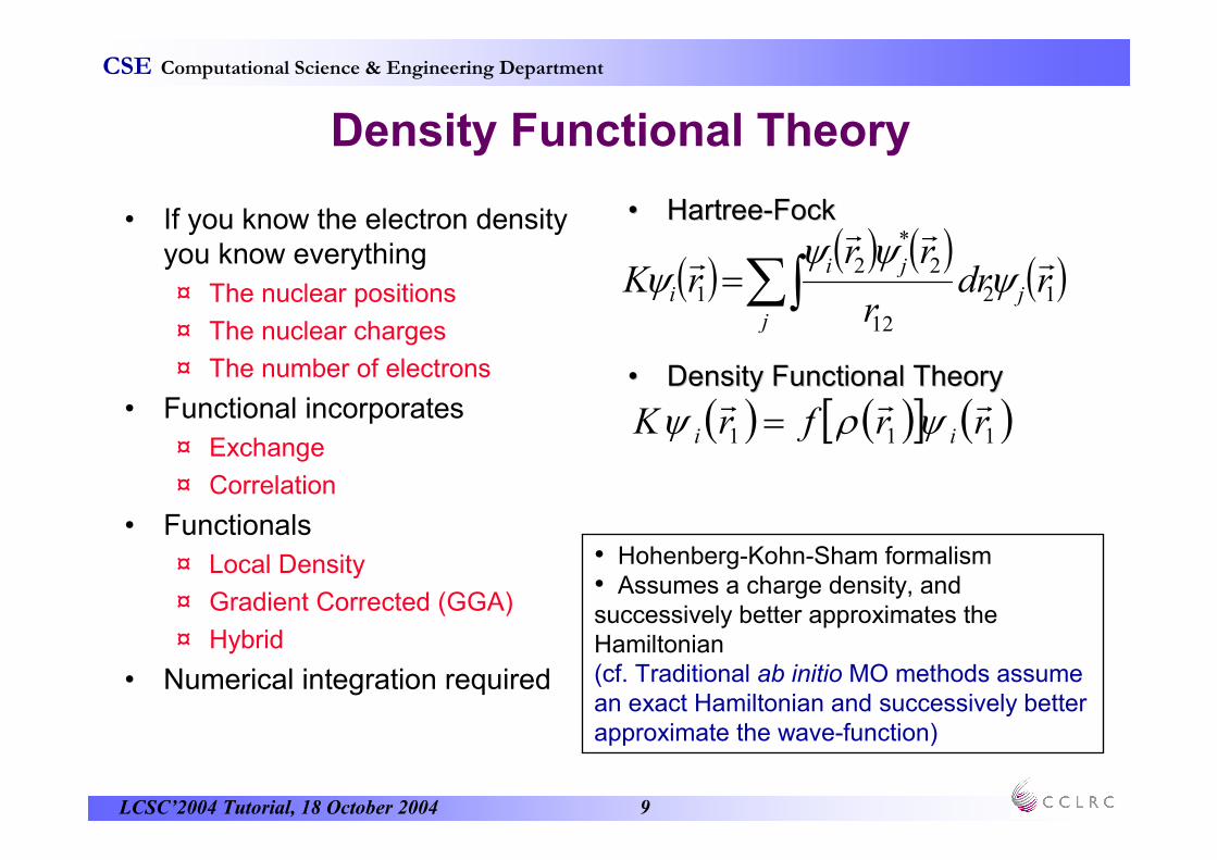
•• HartreeHartree--FockFock
•• Density Functional TheoryDensity Functional Theory
Density Functional Theory
• If you know the electron density you know everything
¤ The nuclear positions
¤ The nuclear charges
¤ The number of electrons
• Functional incorporates
¤ Exchange
¤ Correlation
• Functionals
¤ Local Density
¤ Gradient Corrected (GGA)
¤ Hybrid
• Numerical integration required
( )( ) ( )
( )12
12
2
*
2
1 rdrr
rrrK j
j
ji
i
rrr
rψ
ψψψ ∑∫=
( ) ( )[ ] ( )111 rrfrK ii
rrrψρψ =
• Hohenberg-Kohn-Sham formalism• Assumes a charge density, and successively better approximates the Hamiltonian(cf. Traditional ab initio MO methods assume an exact Hamiltonian and successively better approximate the wave-function)
LCSC’2004 Tutorial, 18 October 2004 10
CSE Computational Science & Engineering Department
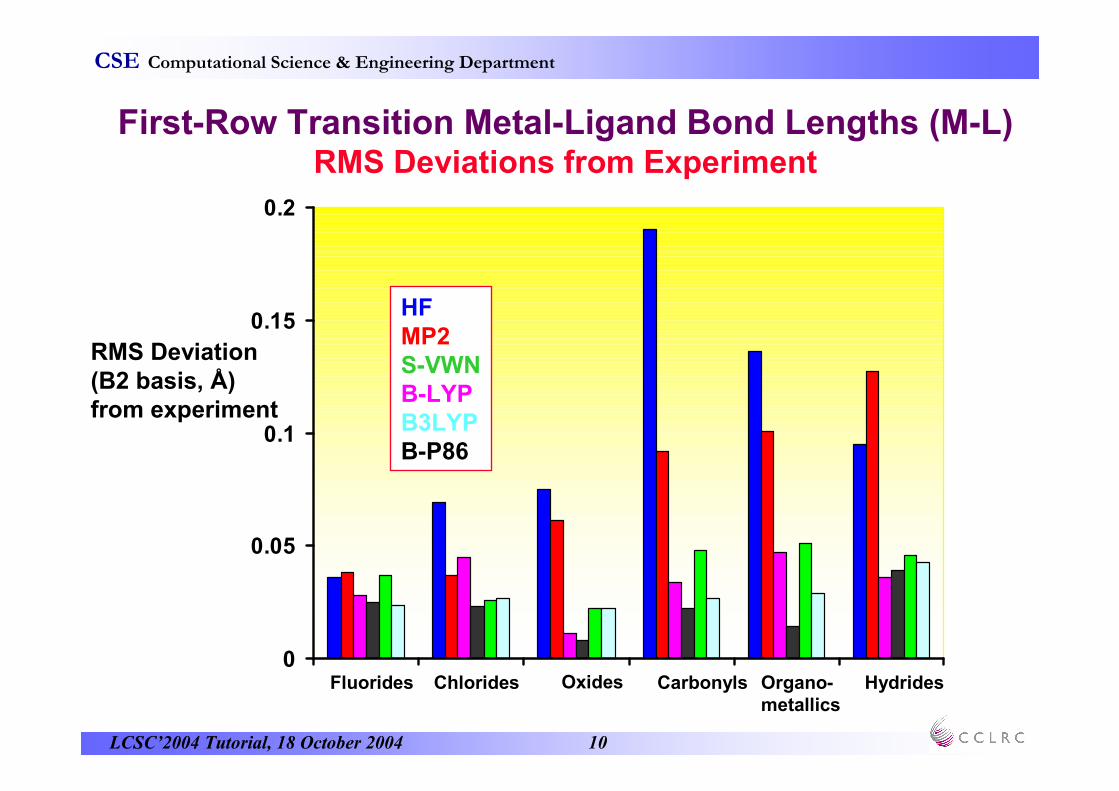
First-Row Transition Metal-Ligand Bond Lengths (M-L)RMS Deviations from Experiment
RMS Deviation(B2 basis, Å) from experiment
0
0.05
0.1
0.15
0.2
OxidesFluorides Chlorides Carbonyls Organo-metallics
Hydrides
HFMP2S-VWNB-LYPB3LYPB-P86
LCSC’2004 Tutorial, 18 October 2004 11
CSE Computational Science & Engineering Department
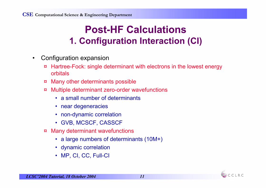
Post-HF Calculations 1. Configuration Interaction (CI)
• Configuration expansion
¤ Hartree-Fock: single determinant with electrons in the lowest energy orbitals
¤ Many other determinants possible
¤ Multiple determinant zero-order wavefunctions
• a small number of determinants
• near degeneracies
• non-dynamic correlation
• GVB, MCSCF, CASSCF
¤ Many determinant wavefunctions
• a large numbers of determinants (10M+)
• dynamic correlation
• MP, CI, CC, Full-CI

LCSC’2004 Tutorial, 18 October 2004 12
CSE Computational Science & Engineering Department
•• ExpandExpand
•• Second order energy Second order energy
Post-HF Calculations 2. Perturbation Theory
• Møller-Plesset 2nd order perturbation theory (MP2) is the most efficient post-HF method
• Size extensive
• Non-variational
• Problems if orbital energies
(εi,εa) close together
• Functionality available
¤ Energy (MP2, MP3)
¤ Gradients (MP2, MP3)
¤ Analytic frequencies (MP2)
¤ Numerical frequencies (MP2, MP3)
• Both direct and conventional MP2 scheme available
∑ −−+=
ijab baji
abijE
εεεε
2
41)2(
K
K
+Ψ+Ψ+Ψ=Ψ
+++=
+=
)2(2)1()0(
)2(2)1()0(
)0( ˆˆˆ
λλ
λλ
λ
EEEE
VHH
LCSC’2004 Tutorial, 18 October 2004 13
CSE Computational Science & Engineering Department
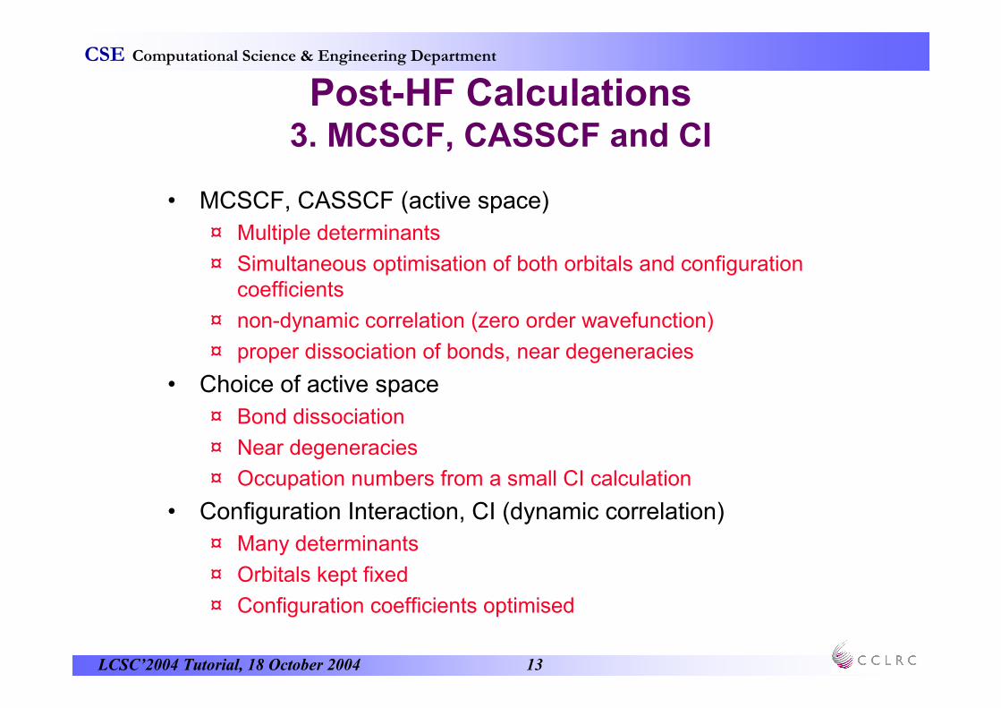
Post-HF Calculations3. MCSCF, CASSCF and CI
• MCSCF, CASSCF (active space)
¤ Multiple determinants
¤ Simultaneous optimisation of both orbitals and configuration coefficients
¤ non-dynamic correlation (zero order wavefunction)
¤ proper dissociation of bonds, near degeneracies
• Choice of active space
¤ Bond dissociation
¤ Near degeneracies
¤ Occupation numbers from a small CI calculation
• Configuration Interaction, CI (dynamic correlation)
¤ Many determinants
¤ Orbitals kept fixed
¤ Configuration coefficients optimised

LCSC’2004 Tutorial, 18 October 2004 14
CSE Computational Science & Engineering Department
Post-HF Calculations 4. MRDCI and Direct-CI
• MRDCI
¤ Computes and stores all (Table-CI) or part (semi-direct) of the Hamiltonian matrix
¤ Perturbatively selects the most important determinants
¤ Useful for calculating excited states and UV/Vis spectra
¤ semi-direct implementation extended size of systems amenable to study - 5 X 10⁵ configurations, 20 roots
¤ “automatic” calculation of UV/Vis spectra
• Direct-CI
¤ Recomputes most of the Hamiltonian matrix whenever needed
¤ Uses all single and double excitations from a multireference set
¤ Useful for calculating accurate ground states
¤ Limited range of Excited states also possible
¤ 107-108 configuration state functions
• Full-CI
¤ Useful for benchmark energies

LCSC’2004 Tutorial, 18 October 2004 15
CSE Computational Science & Engineering Department
Post-HF Calculations 5. Coupled Cluster
• Exponential expansion of the wavefunction
• Size extensive
• Non-variational
• CCSD (n6) and CCSD(T) (n7 scaling)
• At present only closed shell energies available in GAMESS-UK
• Most useful for accurate ground state energies
• Now widely used to obtain accurate energetics from DFT geometries

LCSC’2004 Tutorial, 18 October 2004 16
CSE Computational Science & Engineering Department
Response Theory
• Time independent reference wavefunction
• Response to a time dependent electric field treated with a perturbation expansion
• Eigenvalues of resulting equations correspond to excitation energies
• Most useful as an efficient formalism to calculate UV/Vis spectra, ionisation and attachment potentials
• Accuracy good for single electron excitations
• Tamm-Dancoff Approximation (TDA)
¤ Equivalent to a Singles CI
• Random Phase Approximation (RPA)
¤ Includes some correlation effects with the reference state
¤ Excited state gradient and geometry optimisation
• Multi Configurational Linear Response (MCLR)
¤ RPA using a MCSCF reference wavefunction

LCSC’2004 Tutorial, 18 October 2004 17
CSE Computational Science & Engineering Department
GAMESS-UK
• GAMESS-UK on the web
• Why was GAMESS-UK developed¤ Developments undertaken
• On what hardware platforms does the code currently run
• What is the current functionality in GAMESS-UK and what are the limitations and expectations
• Benchmarks and associated cost-effectiveness
• Who is doing the Developments and Support
LCSC’2004 Tutorial, 18 October 2004 18
CSE Computational Science & Engineering Department
• Capabilities: www.cfs.dl.ac.uk/gamess-uk/
• User’s Manual: www.cfs.dl.ac.uk/docs
• Tutorial (this material): www.cfs.dl.ac.uk/tutorials
• Benchmarks: www.cfs.dl.ac.uk/benchmarks
• Applications: www.cfs.dl.ac.uk/applications
• FAQ’s: www.cfs.dl.ac.uk/FAQ
• Hardware Platforms: www.cfs.dl.ac.uk/hardware
• Bug Reporting: www.cfs.dl.ac.uk/cgi-bin/bugzilla/index.cgi
• Support
WWW Pages for GAMESS-UK

LCSC’2004 Tutorial, 18 October 2004 19
CSE Computational Science & Engineering Department
Why GAMESS-UK was Developed
• Developed as part of CCP1, the collaborative computational project in molecular electronic structure.
• Adopted due to availability of gradient capabilities absent in the ATMOL suite of programs originally maintained by CCP1.
• Derived from the original GAMESS code (HONDO5) obtained in 1981 from Michael Dupuis; then at the National Resource for Computational Chemistry (NRCC) in the US.
• Original code limited to HF/gradient functionality for s, p & d Cartesian Gaussian orbital basis sets, with open- and closed- shell SCF treatments within both the RHF and UHF frameworks.
• Generalised Valence Bond treatment supported.
• Subsequent developments and functionality quite separate from GAMESS-US.
http://www.ccp1.ac.uk

LCSC’2004 Tutorial, 18 October 2004 20
CSE Computational Science & Engineering Department
Original GAMESS Functionality
• Rotation techniques to evaluate repulsion integrals over s and p Gaussians; Rys Polynomial for d.
• SCF convergence controlled via level-shifting, damping and extrapolation.
• Gradients for above wavefunctions evaluated with Schlegel’s algorithm for s and p Gaussians, and RysPolynomial method for d.
• Force constants evaluated by numerical differentiation.
• Ab initio core potentials were provided in a semi-local formalism for performing valence-only molecular orbital treatments.
• Limited range of analysis options & properties
• Limited range of post Hartree-Fock functionality

LCSC’2004 Tutorial, 18 October 2004 21
CSE Computational Science & Engineering Department
Developments I.
• Integral and gradient technology extended to include f and gGaussian functions.
• Limitation to Cartesian basis sets lifted through the provision of spherical-harmonic basis sets.
• SCF controls now use a hybrid scheme of level shifters and DIISmethods.
• Facilities for CASSCF, MCSCF and MP2 and MP3 calculations.
• Geometry optimisation via a quasi-Newton rank-2 update method.
• Transition state location either via synchronous transit, trust region or “hill walking” methods.
• Force constants may be evaluated analytically.
• Valence-only molecular orbital treatments through the incorporation of many ab initio core potentials (both semi- and non-local).

LCSC’2004 Tutorial, 18 October 2004 22
CSE Computational Science & Engineering Department
Wavefunction Analysis and Properties
• Population analysis
• Natural Bond Orbital (NBO)
• Distributed Multipole analysis.
• Localised orbitals.
• Graphical analysis.
• Calculation of 1-electron properties.
• Interface to the AIMPAC code of Bader.
Properties – CPHF Treatments
A range of molecular properties available from coupled Hartree-Fock (CHF) calculations:
• polarisibilities and molecular hyper-polarisibilities.
• infra-red and Raman intensities through the calculation of dipole moments and polarisibility derivatives.
Amos, R. D., 1987, in Adv. Chem. Phys., pp 99
Bieglerkonig, F. W., Bader, R. F.
W. and Tang, T. H., 1982, J.
Comput. Chem., 3, 317-328.
Reed, A. E., Curtiss, L. A. and Weinhold, F.,
1988, Chem. Rev., 88, 899-926.

LCSC’2004 Tutorial, 18 October 2004 23
CSE Computational Science & Engineering Department
Developments II.Expansion of post Hartree-Fock capabilities
• Configuration Interaction (CI) treatment of electronic spectra and related properties using table-driven selectionalgorithms within the framework of MR-DCI calculations.
R.J. Buenker in `Studies in Physical and Theoretical Chemistry', 21
(1982) 17
Krebs, S. and Buenker, R. J., 1995, J. Chem. Phys., 103, 5613-5629.
• Implementation of a semi-direct table-driven MRDCImodule provides more extensive capabilities for treating electronic spectra and related phenomena.
Engels, B., Pleß, V. and Suter, H.-U., Direct MRD-CI, University of
Bonn, Bonn, Germany, 1993.
• Addition of a Direct-CI module to enable the calculation of ground- and excited-states.
Saunders, V. R. and van Lenthe, J. H., 1983, Mol. Phys., 48, 923-
954.

LCSC’2004 Tutorial, 18 October 2004 24
CSE Computational Science & Engineering Department
Developments II.Expansion of post Hartree-Fock capabilities
• Correlation treatments expanded through the incorporation of a Full -CI,
Harrison, R. J. and Zarrabian, S., 1989, Chem. Phys. Lett., 158,
393-398.
and CCSD and CCSD(T) modules (latter limited to closed-shell systems).
Lee, T. J. and Rice, J. E., 1988, Chem. Phys. Lett., 150, 406-415.
Rendell, A. P., Lee, T. J. and Komornicki, A., 1991, Chem. Phys.
Lett., 178, 462-470.
• Incorporation of a size-consistent variant of Multi-reference MP2 theory module with no restriction on CAS wavefunctions (also provides MR-MP3 capabilities).
Roos, B. O., Linse, P., Siegbahn, P. E. M. and Blomberg, M. R. A.,
1982, Chem. Phys., 66, 197-207.

LCSC’2004 Tutorial, 18 October 2004 25
CSE Computational Science & Engineering Department
Developments III.Excited and Ionised States
• Random Phase Approximation (RPA) and Multi-configurational Linear Response (MCLR) capabilities enable the treatment of electronic transition energies and corresponding oscillator strengths.
Fuchs, C., Bonacickoutecky, V. and Koutecky, J., 1993, J. Chem.
Phys., 98, 3121-3140.
• RPA treatments available in both conventional and direct form.
• Direct calculation of molecular valence ionisation energies through Green's function techniques using either outer-valence Green's function (OVGF)
Cederbaum, L. S. and Domcke, W., 1977, Adv. Chem. Phys, 36, 205.
or the two-particle hole Tamm-Dancoff method (2ph-TDA).
Schirmer, J. and Cederbaum, L. S., 1978, J. Phys. B., 11, 1889

LCSC’2004 Tutorial, 18 October 2004 26
CSE Computational Science & Engineering Department
Developments IV. DFT Module
• Development of full-featured DFT module
¤ Access to wide variety of functionals
¤ S-VWN, B-LYP, B-P86, B3-LYP, HCTH, B97, B97-1, B97-2, PBE, EDF1, FT97 etc.
• Evaluation of the energy and gradient of the energy with respect to the nuclear coordinates.
• Can also calculate the second derivatives analytically.
• All terms can be evaluated for GGA functionals.
• Coupled perturbed Kohn-Sham (CPKS) equations solvable for both external field and geometrical perturbations.
• Predefined quadrature schemes developed to easily guarantee results to a particular accuracy.

LCSC’2004 Tutorial, 18 October 2004 27
CSE Computational Science & Engineering Department
Developments V. Solvent Effects
• Place a QM molecule in an environment consisting of other classical molecules and a dielectric media.
¤ VanDuijnen, P. T. and DeVries, A. H., 1996, Int. J. Quantum Chem., 60, 1111-1132.
¤ Devries, A. H., Vanduijnen, P. T., Juffer, A. H., Rullmann, J. A. C., Dijkman, J. P., Merenga, H. and Thole, B. T., 1995, J. Comput. Chem., 16, 1445-1446.
¤ Devries, A. H., Vanduijnen, P. T., Juffer, A. H., Rullmann, J. A. C., Dijkman, J. P., Merenga, H. and Thole, B. T., 1995, J. Comput. Chem., 16, 37-55.
• The classical surroundings may be modelled in a number of ways:
1. by point charges to model the electrostatic field due to the surroundings
2. by polarizabilities to model the (electronic) response of the surroundings
3. by an enveloping dielectric to model bulk response (both static and electronic) of the surroundings, and
4. by an enveloping ionic solution, characterized by its Debye screening length.
Solvent effects can be modelled with the Direct Reaction Field (DRF) technique.

LCSC’2004 Tutorial, 18 October 2004 28
CSE Computational Science & Engineering Department
Developments VI. ZORA, VB etc.
• Relativistic effects included through the Zero'th Order Regular Approximation (ZORA) module.
¤ Important for an accurate treatment of the inner electrons of the heavier elements.
¤ A two component alternative to the full 4 component Dirac equation. While much cheaper than the latter, ZORA recovers a large part of the relativistic effects.
¤ The scalar (1-component) form is now available, with the full 2-component implementation (including spin-orbit coupling) in progress.
¤ Once the effects have been included, all other ab initio, DFT and post-Hartree-Fock methods can be used without change.
• Valence Bond module (Turtle Program)
van Lenthe, J. H., Dijkstra, F. and Havenith, R. W. A., 2002, TURTLE - A
Gradient VBSCF Program, ed. D. Cooper (Amsterdam: Elsevier), pp 79-116
Verbeek, J. and van Lenthe, J. H., 1991, J. Mol. Struct.. (Theochem), 229,
115-137.

LCSC’2004 Tutorial, 18 October 2004 29
CSE Computational Science & Engineering Department
Developments VII.Large Molecules and QM/MM
• Treatment of large Quantum Mechanical Molecules¤ Program is effectively open-ended in direct-SCF, -DFT and -MP2
modes, so that direct SCF calculations on up to 10,000 basis functions have been performed
• QM/MM approaches¤ Treat small “active site” with Quantum Mechanics and the rest of the
molecule with Molecular Mechanics.
• GAMESS-UK integrated into the ChemShell package.
• GAMESS-UK has an interface to the CHARMM (“Chemistry at Harvard Molecular Mechanics package”).
Sherwood, P., de Vries, A. H., Guest, M. F., Schreckenbach, G., Catlow, C. R. A., French, S. A., Sokol, A. A., Bromley, S. T., Thiel, W., Turner, A. J., Billeter, S., Terstegen, F., Thiel, S., Kendrick, J., Rogers, S. C., Casci, J., Watson, M., King, F., Karlsen, E., Sjovoll, M., Fahmi, A., Schafer, A. and Lennartz, C., 2003, J. Mol. Struct. (Theochem), 632, 1-28.

LCSC’2004 Tutorial, 18 October 2004 30
CSE Computational Science & Engineering Department
Hardware Platforms• High-End Machines
¤ IBM-p690+ (AIX 5.2 / CSM) and IBM SP (AIX 5.1D / PSSP 3.4)
¤ Cray T3E (UNICOS/mk 2.0.4.X)
¤ SGI Origin 3000 (IRIX 6.5) and SGI Altix 3700 (Linux64 2.4-21-sgi)
¤ Compaq AlphaServer SC (Tru64 V5.1A)
• Desktop Workstations and Clusters of Workstations
¤ SUN (Solaris 2.6 and 2.8),
¤ IBM (AIX and 5.1 and 5.2),
¤ SGI/R4400 (IRIX5.3), SGI_N32 (IRIX 6.5),
• R8K/R10K/R12K/R14K
¤ DEC Alpha (Compaq Tru64 V5.1, RedHat Linux*)
¤ PowerPC (RedHat Linux*) and Macintosh MAC OS X
¤ HP (HP UX B10.20 and B11.0)
• x86 and IA64 systems and associated Commodity Clusters
¤ Pentium III and 4, AMD Athlon & Opteron, and Itanium-2 (PGI, ifc/efc)
¤ PC (RedHat, Suse etc Linux 2.2.X, 2.4.X SMP, egcs g77/gcc)
Minimum requirements:
128-256 MByte RAM2 GByte disk (SCSI)

LCSC’2004 Tutorial, 18 October 2004 31
CSE Computational Science & Engineering Department
100
77
40
45
54
73
79
113
133
128
117
107
107
72
137
127
136
0 20 40 60 80 100 120 140
IBM p-series 690/1300
IBM p-series 690/1700
HP PA-9000/RP7410-875
SGI Origin3800/R14k-600
SUN FireV880 / 900 Cu
SUN Blade 2000 / 1056 Cu
Compaq Marvel EV7 /1000
Compaq Alpha ES45/1250
AMD Opteron 244/ 1800
AMD Opteron 848/ 2200
Intel Tiger Itanium2/1500
HP RX5670 Itanium2/1500-H
HP RX2600 Itanium2/1500-L
HP RX4640 Itanium2/1300-H
SGI Altix3700 Itanium2/1300
Pentium 4 Xeon / 3066
AMD MP2400+ / 2000
The GAMESS-UK Serial Benchmark Performance relative to the IBM p-series 690/pwr4 1.3 GHz
2.3 minutes

LCSC’2004 Tutorial, 18 October 2004 32
CSE Computational Science & Engineering Department
Support and Development
• GAMESS-UK is maintained, supported and distributed by Computing for Science (CFS) Ltd.
• CFS was founded in the UK in 1992 by an international consortium of established academic and industrial figures in the area of molecular electronic structure and modelling: Drs. M.F. Guest, J.H. van Lenthe, J. Kendrick, and K. Schoeffel.
• Funding provided by a number of agencies in the UK (Research Councils via CCP1) and abroad (NWO, The Netherlands)
• Commercial revenues generated from the code
¤ Sufficient to part fund a support post

LCSC’2004 Tutorial, 18 October 2004 33
CSE Computational Science & Engineering Department
Program Basics
Input file preparation and job execution

LCSC’2004 Tutorial, 18 October 2004 34
CSE Computational Science & Engineering Department
Input Preparation
GAMESS-UK reads a short, directive-structured, input from a data file which can be
¤ (i) prepared by hand using a text editor
¤ (ii) generated by a graphical interface - we will consider two
• CCP1 Python GUI
• MOLDEN
¤ GUI Functionality
• z-matrix (internal coordinate) editing
• graphical data display (e.g. orbitals)
• job submission
¤ None of the graphical interfaces currently support the full functionality. This workshop will concentrate on the input files, with GUIs available and demonstrated in the practical sessions.
LCSC’2004 Tutorial, 18 October 2004 35
CSE Computational Science & Engineering Department
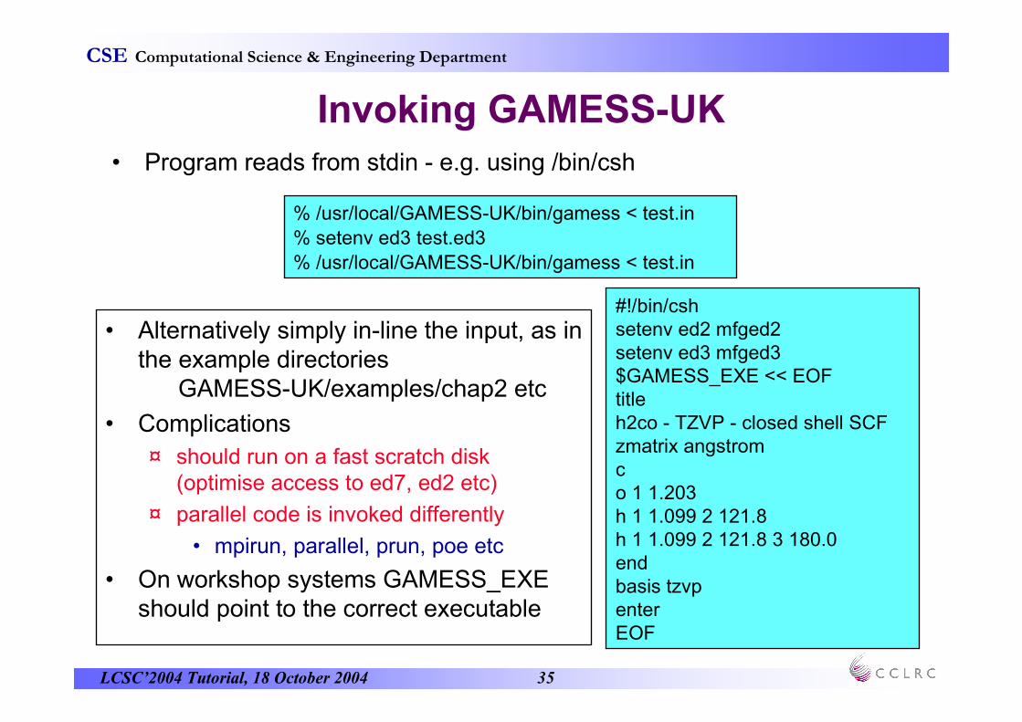
Invoking GAMESS-UK
• Alternatively simply in-line the input, as in the example directories
GAMESS-UK/examples/chap2 etc
• Complications
¤ should run on a fast scratch disk (optimise access to ed7, ed2 etc)
¤ parallel code is invoked differently
• mpirun, parallel, prun, poe etc
• On workshop systems GAMESS_EXE should point to the correct executable
• Program reads from stdin - e.g. using /bin/csh
% /usr/local/GAMESS-UK/bin/gamess < test.in
% setenv ed3 test.ed3
% /usr/local/GAMESS-UK/bin/gamess < test.in
#!/bin/cshsetenv ed2 mfged2setenv ed3 mfged3$GAMESS_EXE << EOFtitleh2co - TZVP - closed shell SCFzmatrix angstromco 1 1.203h 1 1.099 2 121.8h 1 1.099 2 121.8 3 180.0endbasis tzvpenterEOF

LCSC’2004 Tutorial, 18 October 2004 36
CSE Computational Science & Engineering Department
The rungamess Script
• rungamess
¤ creates a scratch directory
¤ sets environment variables from command line arguments
¤ files named <job>.in, <job>.out, <job>.pun etc
• Arguments
-k ed3 keep file on local disk
-k ed3=junk.ed3 keep file as specified name
-t ed7=junk.ed7 keep temporary file (on $GAMESS_TMP)
-p 8 number of parallel processors
-q Submit it a job queue
-r mrdci Keep files needed to restart an MRDCI run (etc)
ed2, ed3, ed7 … Mainfile, Dumpfile, Scratchfile etc

LCSC’2004 Tutorial, 18 October 2004 37
CSE Computational Science & Engineering Department
% rungamess test
% rungamess -p 8 -q test
% rungamess -k ed3 -k ed2=/tmp/ed2 test1
% rungamess -k ed4=test1.ed3 test2
% rungamess -r mrdci test1
% rungamess -r mrdci -n test1 test_restart
rungamess - Examples and Environment Variables
Environment variables
GAMESS_EXE GAMESS-UK executable
GAMESS_SCR routing for scratch directory files
GAMESS_TMP routing for files indicated with -t
GAMESS_PAREXE GAMESS-UK parallel executable
GAMESS_SUBMODE How to submit jobs
ll pbs nqs
GAMESS_PARMODE How to run parallel jobs
mpi sgimpi poe tcgmsg

LCSC’2004 Tutorial, 18 October 2004 38
CSE Computational Science & Engineering Department
Input Structure - A Sample Input
• Predirectives
¤ file routing, parallel options etc, memory allocation
• Directive-structure, keyword driven
¤ Class 1
• title, geometry, basis
¤ Class 2
• runtype, scftype, vectors, enter etc
• Many options have defaults, shown in blue.
• Numerous examples of data input are provided in the user manual
core 4000000
title
h2co - default 3-21G basis - SCF
charge 0
multiplicity singlet
zmatrix angstrom
c
o 1 1.203
h 1 1.099 2 121.8
h 1 1.099 2 121.8 3 180.0
end
basis 3-21g
runtype scf
scftype rhf
thresh 5
vectors atoms
enter 1input0.in, input1.in

LCSC’2004 Tutorial, 18 October 2004 39
CSE Computational Science & Engineering Department
Program Basics
1. Specifying the Geometry and Basis Set

LCSC’2004 Tutorial, 18 October 2004 40
CSE Computational Science & Engineering Department
Specification of Geometry
• Cartesian
¤ Easily obtained from modelling software
¤ Can automatically generate internal coordinates for optimisation
• Z-matrix (internal) coordinates
¤ A way to build a geometry from known bond lengths, angles etc
¤ Can optimise chosen set of internal coordinates
¤ Hessian matrices generally better conditioned

LCSC’2004 Tutorial, 18 October 2004 41
CSE Computational Science & Engineering Department
title
taut 3 3-21g energy = -297.971122 au
geometry au
0.00000 0.00000 0.00000 1.0 h
-1.87385 0.00000 0.00000 7.0 n
-3.15944 -2.29528 0.00000 7.0 n
-3.50408 1.96648 0.00000 6.0 c
-5.53585 -1.64980 0.00000 6.0 c
-5.89182 1.00597 0.00000 6.0 c
-2.87960 3.87928 0.00000 1.0 h
-7.64127 1.98814 0.00000 1.0 h
-7.42454 -3.37843 0.00000 8.0 o
-6.76589 -5.08190 0.00000 1.0 h
end
enter
Geometry input
• Units either atomic units (au) or Angstrom
• Coordinates (x,y,z)
• Charge
¤ positive
¤ negative
¤ fractional
• Tag <symbol><label>
¤ Tag is used to assign basis sets
¤ Tag is used in symmetry determination and analysis
• geometry all¤ Generate internals
geom0.in

LCSC’2004 Tutorial, 18 October 2004 42
CSE Computational Science & Engineering Department
• Define parameters
• Use of symbolic variables and constants
• Z-matrix conventions: First atom will be at (0,0,0), Secondat (0,0,z), Third at (x,0,z)
Each nucleus (including dummies) is numbered sequentially and specified on a single data line. Nthnucleus (N>3):
TAGN, N1, R1, N2, ANG12, N3, ANG123, ITYPETAGN - name and chemical nature of the nucleusN1 - an integer specifying a previously defined nucleusR1 - R(N-N1) in the appropriate units.N2 - an integer specifying a second nucleus, N2, different from N1, for which the angle (N,N1,N2) will be given.ANG12 - value of (N,N1,N2), the internuclear angle at N1 between N and N2, in degrees. N3 - an integer specifying a nucleus for which the dihedral angle (N,N1,N2,N3) will be defined as ANG123.ANG123 - the internuclear dihedral angle (N,N1,N2,N3) specified (º). It is the angle between the planes (N,N1,N2) and (N1,N2,N3)(sign)
Z-matrix input
TITLE
MoF6 Oh symmetry
ZMAT ANGSTROMMOF 1 MOFF 1 MOF 2 90.0F 1 MOF 2 90.0 3 90.0F 1 MOF 2 90.0 3 180.0F 1 MOF 2 90.0 3 -90.0F 1 MOF 3 90.0 2 180.0VARIABLESMOF 1.814END
zmat1.in
LCSC’2004 Tutorial, 18 October 2004 43
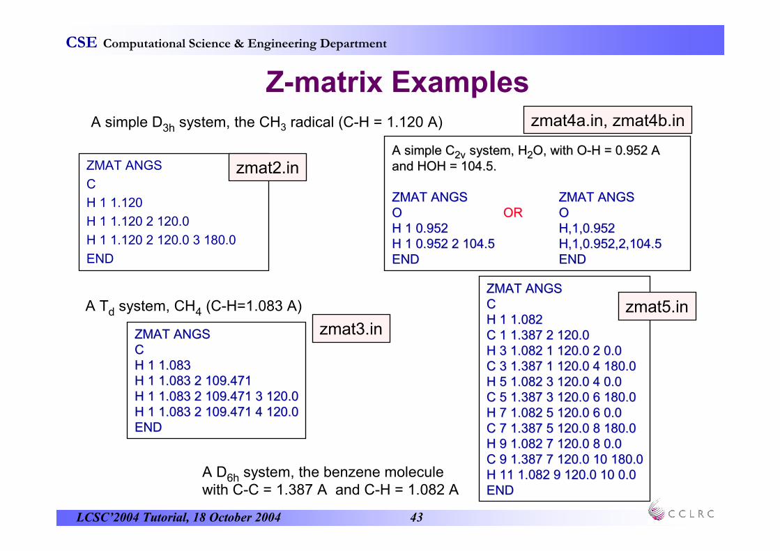
CSE Computational Science & Engineering Department
ZMAT ANGS
C
H 1 1.120
H 1 1.120 2 120.0
H 1 1.120 2 120.0 3 180.0
END
Z-matrix Examples
A simple CA simple C2v2v system, Hsystem, H22O, with OO, with O--H = 0.952 A H = 0.952 A
and HOH = 104.5.and HOH = 104.5.
ZMAT ANGSZMAT ANGS ZMAT ANGS ZMAT ANGS OO OROR OOH 1 0.952H 1 0.952 H,1,0.952H,1,0.952H 1 0.952 2 104.5H 1 0.952 2 104.5 H,1,0.952,2,104.5H,1,0.952,2,104.5ENDEND END END
A simple D3h system, the CH3 radical (C-H = 1.120 A)
ZMAT ANGSZMAT ANGSCCH 1 1.083H 1 1.083H 1 1.083 2 109.471H 1 1.083 2 109.471H 1 1.083 2 109.471 3 120.0H 1 1.083 2 109.471 3 120.0H 1 1.083 2 109.471 4 120.0H 1 1.083 2 109.471 4 120.0ENDEND
A Td system, CH4 (C-H=1.083 A)ZMAT ANGSZMAT ANGSCCH 1 1.082H 1 1.082C 1 1.387 2 120.0C 1 1.387 2 120.0H 3 1.082 1 120.0 2 0.0H 3 1.082 1 120.0 2 0.0C 3 1.387 1 120.0 4 180.0C 3 1.387 1 120.0 4 180.0H 5 1.082 3 120.0 4 0.0H 5 1.082 3 120.0 4 0.0C 5 1.387 3 120.0 6 180.0C 5 1.387 3 120.0 6 180.0H 7 1.082 5 120.0 6 0.0H 7 1.082 5 120.0 6 0.0C 7 1.387 5 120.0 8 180.0C 7 1.387 5 120.0 8 180.0H 9 1.082 7 120.0 8 0.0H 9 1.082 7 120.0 8 0.0C 9 1.387 7 120.0 10 180.0C 9 1.387 7 120.0 10 180.0H 11 1.082 9 120.0 10 0.0H 11 1.082 9 120.0 10 0.0ENDEND
A D6h system, the benzene moleculewith C-C = 1.387 A and C-H = 1.082 A
zmat2.in
zmat3.in
zmat4a.in, zmat4b.in
zmat5.in

LCSC’2004 Tutorial, 18 October 2004 44
CSE Computational Science & Engineering Department
Z-matrix restrictions: Dummy atoms
• Atoms must be specified in terms of previously defined atoms
• Directly-bonded angle ANG12 must be in the range 0 < ANG12 < 180
• Sometimes definition is easier or more reliable using dummy atoms
titlefe(co)5 SCF energyzmat angstromfec 1 rceqx 2 1.00 1 90o 2 rco 3 90 1 180....
constantsrceq 1.8273000rcax 1.8068000rco 1.1520endruntype scfenterFe C O
X
11 22
33
44
ANG12
zmat6.in
LCSC’2004 Tutorial, 18 October 2004 45
CSE Computational Science & Engineering Department
Treatment of Symmetry I.
• the molecular level: the program will deduce the point group symmetry based on the geometry provided
• in default, use that information in minimising the number of integrals that need be computed e.g. in SCF calculations.
• The program is capable of handling both Abelian (e.g. C2v) and non-Abelian point groups (e.g. C3v) on an equal footing
• the orbital level: both at the AO and MO level, when the symmetry characteristics of MOs will be used in optimising both HF and post HF calculations.
• This requirement is met through the use of symmetry-adapted basis functions. While this technique is limited to Abelian point groups, the program will treat non-Abeliangroups by resorting to the optimum Abelian group when handling orbital symmetry (e.g. C3v to Cs )
Before considering aspects of data specification, it is importanBefore considering aspects of data specification, it is important to have t to have
an idea of the methods used in the treatment of molecular symmetan idea of the methods used in the treatment of molecular symmetry. ry.
The aim is to try and optimise performance while maintaining simThe aim is to try and optimise performance while maintaining simplicity plicity
of related data specification. There are of related data specification. There are two levelstwo levels at which symmetry at which symmetry
is employed;is employed;

LCSC’2004 Tutorial, 18 October 2004 46
CSE Computational Science & Engineering Department
Treatment of Symmetry II.
• The TAGs used to characterise the component nuclei of the system in either the GEOMETRY or ZMATRIX directive play a vital role in symmetry determination. They are used to establish the effective point group symmetry of the system. Failure to appreciate the rules for TAG specification can lead to a considerable loss in efficiency.
• In RHF, UHF and Moller Plesset calculations GAMESS-UK will, based on the molecular point group, generate and retain only the unique integrals required, for example, in the process of constructing a`skeletonised' Fock matrix.
• Such a symmetry-truncated integral list is, however, NOT usable at present in pair-GVB, CASSCF, MCSCF, RPA or CI calculations, and again considerable caution should be taken when using an integral file generated in an earlier SCF run in a subsequent post-HF calculation using the BYPASS directive.
• In geometry optimisations the point group is derived from the starting geometry, and is not allowed to change during the subsequent optimisation. This can lead to problems if the Z-matrix is constructed in such a way as to allow such changes to occur.
• Both MCSCF and CI modules assume that symmetry adaptation is in operation. If for any reason the SCF MOs of differing irreducible representations become mixed, the post HF calculations may prove unreliable.

LCSC’2004 Tutorial, 18 October 2004 47
CSE Computational Science & Engineering Department
Controlling the Point Group Symmetry
In some instances the user need consider lowering the point group determined in default by the program, particularly in the case of degenerate point groups, which for some SCFTYPEs and RUNTYPEs must be a subset of the D2h group. Specifically the appearance of the message.
***************************************************************** The molecular point group prohibits use of either
* the requested SCFTYPE or RUNTYPE. Reduce the
* molecular symmetry by modifying the nuclear TAGs
****************************************************************
The symmetry handling routines within GAMESS-UK assume that any centres with differing TAGs are not related by symmetry. The point group actually adopted in the calculation may be controlled though appropriate TAG specification.
NbCl5 DNbCl5 D3h3h; changing the ; changing the
first equatorialfirst equatorial
chlorine TAG (to CL1) will chlorine TAG (to CL1) will
yield a Cyield a C2v2v point group, point group,
thus;thus;
ZMAT ANGSTROMZMAT ANGSTROMNBNBCL1 1 REQCL1 1 REQX 2 1.0 1 90X 2 1.0 1 90CL 1 REQ 2 120 3 180CL 1 REQ 2 120 3 180CL 1 REQ 2 120 3 0CL 1 REQ 2 120 3 0CL 1 RAX 2 90 3 90CL 1 RAX 2 90 3 90CL 1 RAX 2 90 3 CL 1 RAX 2 90 3 --9090CONSTANTSCONSTANTSREQ 2.338REQ 2.338RAX 2.362RAX 2.362ENDEND
symmetry1a.in, symmetry1b.in

LCSC’2004 Tutorial, 18 October 2004 48
CSE Computational Science & Engineering Department
Disabling use of Symmetry
nosym
to disable use of symmetry at the molecular level, as this ensures that the calculation will be performed with the input molecular orientation (ensuring properties such as orbitals, dipole moments etc will be in the input frame).
adapt off
can be presented to disable symmetry adaption if symmetry breaking distortions are expected (e.g. QM/MM).
In some applications it is beneficial to present the directives NOSYMNOSYM and “ADAPT OFFADAPT OFF”:
This may lead to a substantial cost penalty for post-HF calculations on symmetric systems!
LCSC’2004 Tutorial, 18 October 2004 49
CSE Computational Science & Engineering Department
Basis Set Specification
• Default Cartesian angular functions (1s, 3p, 6d, 10f, 15g) are used throughout GAMESS-UK.
• Option of using spherical-harmonic (5d, 7f, 9g) angular functions is available through specification of the HARMONIC directive.
¤ This is implemented internally through appropriate transformations, and not by computing integrals or derivative integrals over the spherical functions.
• Default basis set is 3-21G if no input provided
• Variety of mechanisms for specifying basis sets through the BASIS directive
• Explicit and hybrid basis sets are available
• Can be selected from the “internal” Library file
¤ single keyword specification
• BASIS TZVP
• Can be input in general form

LCSC’2004 Tutorial, 18 October 2004 50
CSE Computational Science & Engineering Department
Internal Basis Sets
• Wide variety of internal basis sets can be requested through single keyword specification
¤ BASIS codename
• Minimal Basis
¤ STOnG, MINI
• Split valence (SV)
¤ n-m1G
• Double-zeta (DZ)
• Triple-zeta (TZV) and Extended
• Polarisation basis sets
• Correlation-consistent basis sets (CC-PVDZ, CC-PVTZ, CC-PVQZ, CC-PV5Z).
• ECP basis sets
• DFT Basis sets (DZVP, DZVP2 and TZVP)
Using the same family of basis set for all atoms in the molecule. Examples:
BASIS STO3G
BASIS 6-31G or BASIS SV 6-31G
BASIS DZ
or BASIS DZ AHLRICHS
BASIS DZP
or BASIS DZP AHLRICHS
BASIS TZVP
BASIS 6-311G*
BASIS CC-PVDZ
BASIS ECP STRLC
BASIS DFT DZVP2 basis0.in

LCSC’2004 Tutorial, 18 October 2004 51
CSE Computational Science & Engineering Department
Internal Basis Sets - Hybrid Specification
• Request basis sets from more than one of the “built-in” basis sets
• User is responsible for allocating such a basis to each centre using the centre TAGs as specified in the GEOMETRY or ZMATRIX directive
BASIS
basis1 <TAG1>
basis2 <TAG2>
END
• Only the unique TAGs should be specified in this process
• Examples:
zmatrix angstrom
c
o 1 1.203
h 1 1.099 2 121.8
h 1 1.099 2 121.8 3 180.0
end
basis
tzv h
tzvp o
tzvp c
end
basis
sv h 3-21g
sv o 6-31g*
sv c 6-31g*
end
basis1a.in
basis1b.in

LCSC’2004 Tutorial, 18 October 2004 52
CSE Computational Science & Engineering Department
BASIS
S H
0.032828 13.3615
0.231208 2.0133
0.817238 0.4538
S H
1.0 0.1233
S C
0.002090 4232.61
0.015535 634.882
0.075411 146.097
0.257121 42.4974
0.596555 14.1892
0.242517 1.9666
S C
1.0 5.1477
S C
1.0 0.4962
S C
1.0 0.1533
P C
0.018534 18.1557
0.1154420 3.9864
0.3862060 1.1429
0.6400890 0.3594
P C
1.0 0.1146
END
General Basis Set Input
title
CH2 3B1 GRHF open shell
mult 3
zmatrix angstrom
c
h 1 1.071
h 1 1.071 2 128.65
end
Compatibility is also provided with other QC packages (NWChem, Gaussian) by accepting a reversed ordering of coefficients / exponents in the basis definition lines
Coefficient ofCoefficient of
gaussiangaussian primitiveprimitive Exponent ofExponent of
gaussiangaussian primitiveprimitive
basis2a.in
basis2b.in
LCSC’2004 Tutorial, 18 October 2004 53
CSE Computational Science & Engineering Department
Program Basics
2. SCF and DFT Calculations
• RUNTYPE and SCFTYPE• SCF Input• Wavefunctions• Initial MO vectors• Direct and conventional SCF algorithms• DFT• Analysing the Wavefunction• Convergence, files, and restarting

LCSC’2004 Tutorial, 18 October 2004 54
CSE Computational Science & Engineering Department
RUNTYPE specifications
RUNTYPE (and SCFTYPE) define the computation to be carried out.
RUNTYPE defines the particular task to be undertaken;
Default RUNTYPE is SCFi.e., perform a single point SCF calculation
RUNTYPE SCF
RUNTYPE TaskINTEGRAL Single point integral calculation
SCF Single point SCF calculation
OPTIMIZE Geometry optimisation (internals)
OPTXYZ Geometry optimisation (cartesians)
SADDLE Saddle point location
ANALYSE Wavefunction analysis
FORCE Force constant evaluation
HESSIAN Analytic Force constant evaluation
POLARISABILITY Polarisability calculation
HYPER Hyperpolarisability calculation
MAGNET Magnetisability calculation
RAMAN Calculation of Raman Intensities
INFRARED Calculation of IR intensities
TRANSFORM Integral transformation
CI CI calculation
GF Green's Function OVGF calculation
TDA Green's Function 2ph-TDA calculation
RESPONSE Response calc. of Excitation Energies

LCSC’2004 Tutorial, 18 October 2004 55
CSE Computational Science & Engineering Department
SCFTYPE specifications
• SCFTYPE specifies the form of wavefunction calculation to be employedthroughout the nominated task.
SCFTYPE <wavefunction>
• Energies and gradients
¤ Closed-shell (RHF)
¤ Spin-restricted, high-spin open-shell (GRHF)
¤ Spin-unrestricted open-shell (UHF)
¤ Generalised Valence Bond (GVB)
• Finite point groups
• 700 functions should be possibleon PCs / workstations
• 3000 functions should be routine onparallel machines e.g. IBM p690+
¤ About 10,00 functions, 400 atoms have been run
¤ Both GVB and GRHF calculations are performed under the same GVB module
SCFTYPE WavefunctionRHF Restricted Hartree-Fock
UHF Unrestricted Hartree-Fock
GVB Generalised Valence Bond
& high-spin open-shell (GRHF)
MP2 2nd order Moller Plesset
MP3 3nd order Moller Plesse
CASSCF Complete Active Space SCF
MCSCF 2nd order MCSCF
Direct SCF WavefunctionsDIRECT RHF Direct-SCF
or simply DIRECT
DIRECT UHF Direct-UHF
DIRECT GVB Direct-GVB
LCSC’2004 Tutorial, 18 October 2004 56
CSE Computational Science & Engineering Department
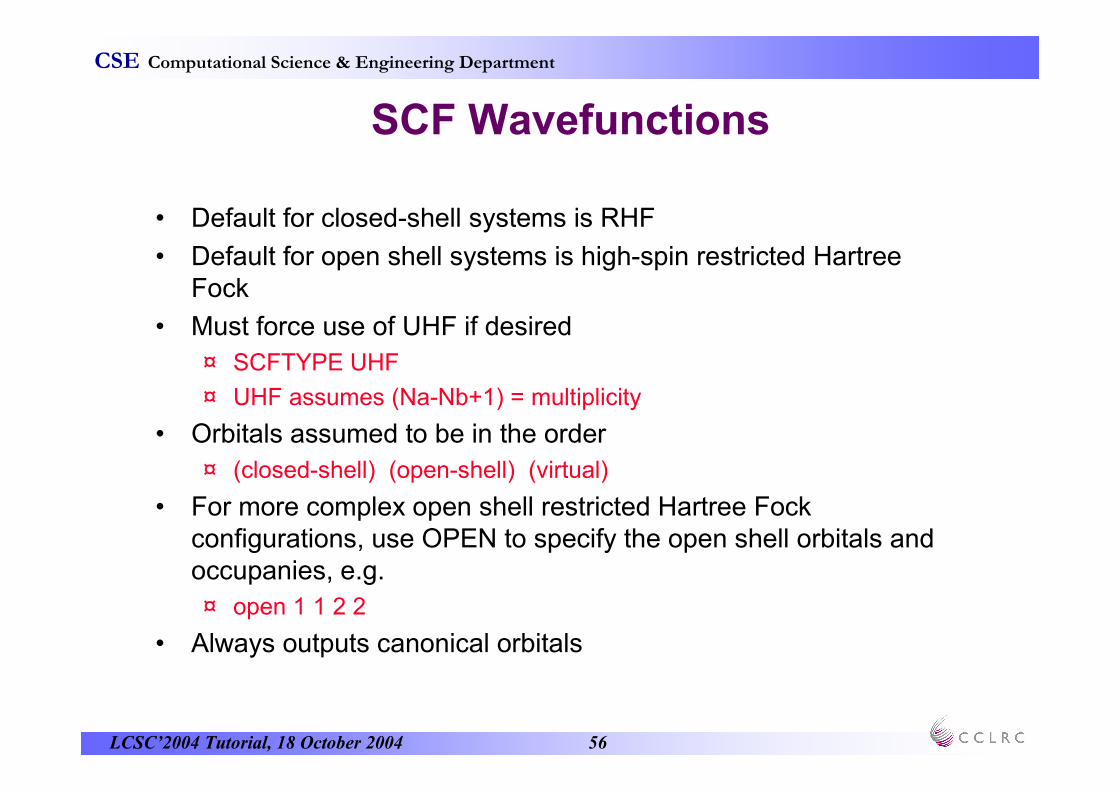
SCF Wavefunctions
• Default for closed-shell systems is RHF
• Default for open shell systems is high-spin restricted HartreeFock
• Must force use of UHF if desired
¤ SCFTYPE UHF
¤ UHF assumes (Na-Nb+1) = multiplicity
• Orbitals assumed to be in the order
¤ (closed-shell) (open-shell) (virtual)
• For more complex open shell restricted Hartree Fockconfigurations, use OPEN to specify the open shell orbitals and occupanies, e.g.
¤ open 1 1 2 2
• Always outputs canonical orbitals

LCSC’2004 Tutorial, 18 October 2004 57
CSE Computational Science & Engineering Department
SCF Input
• Intended that default settings should be sufficient
• Defaults
¤ Restricted-spin wavefunction
¤ Accuracy suitable for non-floppy molecule geometry optimization
¤ Symmetry as deduced from the geometry
• Minimal input (all defaults)
• Performs a closed-shell SCF on the formaldehyde molecule in a 6-31G* basis
title
h2co - 6-31g* basis
zmatrix angstrom
c
o 1 1.203
h 1 1.099 2 121.8
h 1 1.099 2 121.8 3 180.0
end
basis 6-31g*
enter
scf1.in

LCSC’2004 Tutorial, 18 October 2004 58
CSE Computational Science & Engineering Department
Simple Open Shell Examples
title
CH2 3B1 RHF high spin
mult 3
zmatrix angstrom
c
h 1 1.071
h 1 1.071 2 128.65
end
basis 6-31g*
enter
title
CH2 3B1 UHF
mult 3
zmatrix angstrom
c
h 1 1.071
h 1 1.071 2 128.65
end
basis 6-31g*
scftype uhf
enter
3B1 CH2 GRHF 3B1 UHF SCF 1B1 CH2 GRHF
title
CH2 1B1 open shell
mult 1
zmatrix angstrom
c
h 1 1.071
h 1 1.071 2 128.65
end
basis 6-31g*
scftype gvb
open 1 1 1 1
enterscf2a.in
scf2b.in scf2c.in

LCSC’2004 Tutorial, 18 October 2004 59
CSE Computational Science & Engineering Department
Default MO Guess
• Superposition of atomic densities - default
¤ Performs atomic SCF on each atom
¤ Spherically averages occupations
¤ Nearly always the best guess
• When does atomic guess fail?
¤ Some ECPs
¤ Many calculations on metals, especially open d/f shells
¤ Diffuse basis sets
¤ Some DFT calculations
• Other Approaches
¤ Use eigenvectors from a related calculation
¤ Restore from the same or previous Dumpfile (GETQ directive)
• vectors stored in default sections, or in response to section specified on ENTER

LCSC’2004 Tutorial, 18 October 2004 60
CSE Computational Science & Engineering Department
Guess from Smaller MOs
• Projection guess
• use the MOs from a smaller basis as a guess
• e.g., H2CO 6-31G guess for 6-31G** calculation
• vectors reside on the Dumpfile
• vectors from the 6-31G calculation are retrieved in the larger calculation
• use of the GETQ directive that points to the location of the 6-31G vectors on the “foreign” dumpfile (allocated using ed4).
¤ This requires both location and vector section specification
title
h2co - 6-31G basis
zmatrix angstrom
c
o 1 1.203
h 1 1.099 2 121.8
h 1 1.099 2 121.8 3 180.0
end
basis 6-31g
enter
titletitleh2co h2co -- 66--31G** basis31G** basiszmatrixzmatrix angstromangstromcco 1 1.203o 1 1.203h 1 1.099 2 121.8h 1 1.099 2 121.8h 1 1.099 2 121.8 3 180.0h 1 1.099 2 121.8 3 180.0endendbasis 6basis 6--31g**31g**vectors vectors getqgetq ed4 1 1ed4 1 1enterenter
scf3a.in
scf3b.in

LCSC’2004 Tutorial, 18 October 2004 61
CSE Computational Science & Engineering Department
Conventional and Direct SCF
• Conventional SCF is the default
• Formats for storage of the 2e-integral files
• P-supermatrix (closed shells)
• J+K supermatrix (open shells)
• 2e-integral format (all SCFTYPEs)
¤ supermatrix is “fastest” for small cases (< 120 GTOs)
¤ 2e-integral format the default for larger cases, with the file ≤ 3 times smaller than the corresponding supermatrix file
¤ care required when same integral file in different SCF calcs.
• To force direct
¤ SCFTYPE DIRECT RHF
• Disk space and elapsed times suggest avoiding use of conventional SCF for large (> 400 GTOs) cases, except:
¤ using memory to hold integrals on “large” parallel machines (64+CPUs)

LCSC’2004 Tutorial, 18 October 2004 62
CSE Computational Science & Engineering Department
Density Functional Theory
closed-shell DFT calculation
TITLE
H2CO - 3-21G DFT (B-LYP DEFAULT)
ZMATRIX ANGSTROM
C
O 1 1.203
H 1 1.099 2 121.8
H 1 1.099 2 121.8 3 180.0
END
DFT
ENTER
open-shell unrestricted UKS
TITLE
H2CO+ - 2B1 - 3-21G BASIS UKS
CHARGE 1
MULT 2
ZMATRIX ANGSTROM
C
O 1 1.203
H 1 1.099 2 121.8
H 1 1.099 2 121.8 3 180.0
END
SCFTYPE UHF
DFT
ENTER
Input for a DFT calculation is essentially that for the corresponding closed-shell RHF or UHF module, with additional keywords that control the DFT specific features. In the simplest case, the user need just introduce a single data with the character string DFT in the first data field to request a DFT rather than HF calculation:
There is no restricted RKS for open-shell systems,only UKS
dft1a.in
dft1b.in

LCSC’2004 Tutorial, 18 October 2004 63
CSE Computational Science & Engineering Department
DFT Calculations I.
DFT Directive Specification
DFT B-LYP QUADRATURE MEDIUM
or
DFT BECKE88
DFT LYP
DFT QUADRATURE MEDIUM
If the DFT module is switched on without specifying any options then the
following functional and quadrature settings will apply;
• the Becke (1988) exchange functional• the Lee, Yang and Parr (LYP) correlation functional• quadrature grids designed to obtain a relative error of less than 1.0e-6 in the number of electrons per atom. These grids are constructed from the logarithmic radial grid and Gauss-Legendre angular grid, using the SSF weighting scheme with screening and MHL angular grid pruning. (“QUADRATURE MEDIUM" ). • the gradient of the energy will be evaluated without considering the gradient of the quadrature weights and grid points ( "GRADQUAD OFF”).
Most important DFT DirectivesMost important DFT Directives
•• The functionalThe functional
•• Accuracy of the numericalAccuracy of the numerical
integrationintegration
-- Low, Medium, High, Very HighLow, Medium, High, Very High
•• Gradients of the Gradients of the quadraturequadrature
LCSC’2004 Tutorial, 18 October 2004 64
CSE Computational Science & Engineering Department
DFT Calculations II.Specification of Common Functionals
B3LYP; selects the hybrid exchange-correlation energy functional due to Becke.
S-VWN or SVWN; selects the LDA exchange functional and the Vosko, Wilk, and Nusair(VWN) correlation functional.
B-LYP or BLYP; selects the Becke88 exchange energy functional and the Lee, Yang and Parr correlation energy functional.
B-P86 or BP86; selects the Becke88 exchange energy functional and the Perdew 1986 gradient corrected correlation functional.
B97; selects the Becke97 hybrid exchange-correlation energy functional
B97-1; selects the Becke97 hybrid exchange-correlation energy functional as re-parametrised by Hamprecht et al.
HCTH; selects the Hamprecht, Cohen, Tozer & Handy exchange-correlation functional
Specification of Integration GridsSpecification of Integration Grids
Specify the required grid accuracy
DFT QUADRATURE LOW
The LOW accuracy grid should only be used for preliminary studies; designed to obtain the total number of electrons from the density integration with a relative error of 10-4 per atom.
DFT QUADRATURE MEDIUM
The MEDIUM accuracy grid - obtains a relative error of less than 10-6 in the Ne per atom.
DFT QUADRATURE HIGH
The HIGH accuracy grid - obtains a relative error of less than 10-8 in the Ne per atom.
DFT QUADRATURE VERYHIGH
… only for benchmark calculations.
LCSC’2004 Tutorial, 18 October 2004 65
CSE Computational Science & Engineering Department
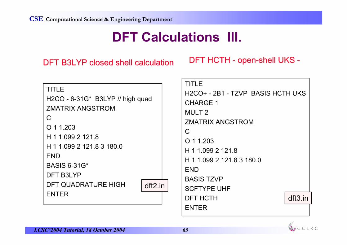
DFT Calculations III.
TITLE
H2CO - 6-31G* B3LYP // high quad
ZMATRIX ANGSTROM
C
O 1 1.203
H 1 1.099 2 121.8
H 1 1.099 2 121.8 3 180.0
END
BASIS 6-31G*
DFT B3LYP
DFT QUADRATURE HIGH
ENTER
TITLE
H2CO+ - 2B1 - TZVP BASIS HCTH UKS
CHARGE 1
MULT 2
ZMATRIX ANGSTROM
C
O 1 1.203
H 1 1.099 2 121.8
H 1 1.099 2 121.8 3 180.0
END
BASIS TZVP
SCFTYPE UHF
DFT HCTH
ENTER
DFT B3LYP closed shell calculationDFT B3LYP closed shell calculation DFT HCTH DFT HCTH -- openopen--shell UKS shell UKS --
dft2.in
dft3.in

LCSC’2004 Tutorial, 18 October 2004 66
CSE Computational Science & Engineering Department
Program Basics
3. Geometry Optimisation
LCSC’2004 Tutorial, 18 October 2004 67
CSE Computational Science & Engineering Department
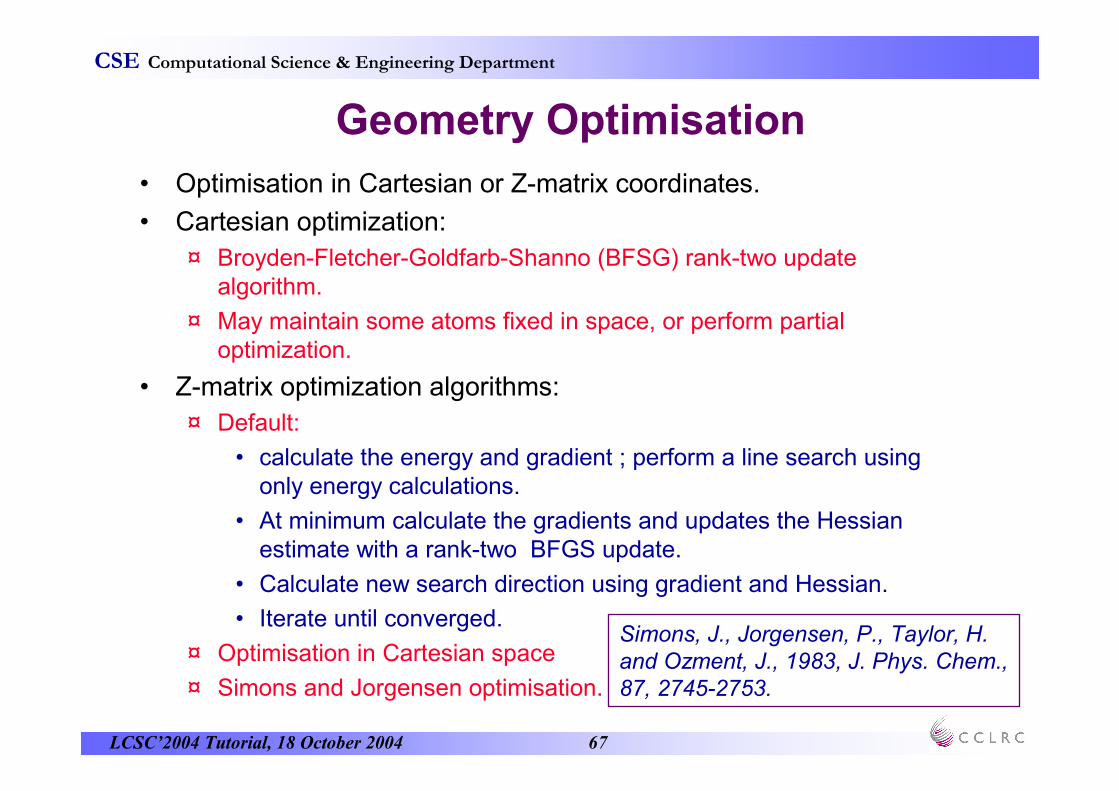
Geometry Optimisation
• Optimisation in Cartesian or Z-matrix coordinates.
• Cartesian optimization:
¤ Broyden-Fletcher-Goldfarb-Shanno (BFSG) rank-two update algorithm.
¤ May maintain some atoms fixed in space, or perform partial optimization.
• Z-matrix optimization algorithms:
¤ Default:
• calculate the energy and gradient ; perform a line search using only energy calculations.
• At minimum calculate the gradients and updates the Hessian estimate with a rank-two BFGS update.
• Calculate new search direction using gradient and Hessian.
• Iterate until converged.
¤ Optimisation in Cartesian space
¤ Simons and Jorgensen optimisation.
Simons, J., Jorgensen, P., Taylor, H.
and Ozment, J., 1983, J. Phys. Chem.,
87, 2745-2753.

LCSC’2004 Tutorial, 18 October 2004 68
CSE Computational Science & Engineering Department
Geometry Optimisation
• Several available Transition state searches available:
¤ Cerjan and Miller algorithm with Murtagh-Sargent or Powell Hessian update (requires an initial Hessian estimate).
¤ Modified version of Bell and Crighton's Quadratic Synchronous Transit (QST) algorithm.
• Convergence determined by 4 criteria:
¤ Largest predicted step in any coordinate.
¤ Average predicted step.
¤ Largest gradient value.
¤ Average gradient value.
Transition State Location
Bell, S. and Crighton, J. S., 1984, J. Chem. Phys., 80, 2464-2475.
Cerjan, C. J. and Miller, W. H., 1981, J. Chem. Phys., 75, 2800-2806.

LCSC’2004 Tutorial, 18 October 2004 69
CSE Computational Science & Engineering Department
Geometry Optimisation
1. the recommended method, a quasi-Newton rank-2 update procedure,
is driven through the specification
RUNTYPE OPTIMIZE
Performs optimisation in internal co-ordinates, and thus requires initial ZMATRIX and VARIABLES specification of the molecular geometry, or ZMATRIX construction from a set of cartesian co-ordinates supplied under control of the GEOMETRY directive.
2. the second internal coordinate-driven method is that based on the hill-walking algorithm due to Simons and Jorgensen. Intended primarily for transition state usage, it may also be employed in geometry optimisation. The procedure is driven through additional keyword specification on the RUNTYPE directive, thus;
RUNTYPE OPTIMIZE JORGENSEN
3. the third method, perhaps less robust and flexible than the others, is a cartesian-driven update method. This is requested through
RUNTYPE OPTXYZ

LCSC’2004 Tutorial, 18 October 2004 70
CSE Computational Science & Engineering Department
Internal Co-ordinates and VARIABLES
RUNTYPE OPTIMIZE
Geometry optimisation is conducted in a system of internal coordinates - bond lengths, bond angles and dihedral angles - defined by the z-matrix.
This is controlled through the introduction of so-called VARIABLES in the z-matrix. Any internal coordinate whose value is to be varied during optimisation must be specified as a VARIABLE, and an initial value assigned to it through the VARIABLE definition lines of the ZMATRIX directive.
Consider the data from the SCF computations on formaldehyde:
ZMATRIX ANGSTROM
C
O 1 1.203
H 1 1.099 2 121.8
H 1 1.099 2 121.8 3 180.0
END
ZMATRIX required when optimising the geometry
ZMATRIX ANGSTROM
C
O 1 CO
H 1 CH 2 HCO
H 1 CH 2 HCO 3 180.0
VARIABLES
CO 1.203
CH 1.099
HCO 121.8
END

LCSC’2004 Tutorial, 18 October 2004 71
CSE Computational Science & Engineering Department
Simple Optimisation Examples
TITLE
H2CO - DZ - OPTIMISATION
ZMATRIX ANGSTROM
C
O 1 CO
H 1 CH 2 HCO
H 1 CH 2 HCO 3 180.0
VARIABLES
CO 1.203
CH 1.099
HCO 121.8
END
BASIS DZ
RUNTYPE OPTIMIZE
ENTER
X1A1 H2COTITLETITLE
H2CO GEOMETRY TESTH2CO GEOMETRY TEST
GEOMETRY GEOMETRY
0.0000000 0.0000000 0.9998722 6 C0.0000000 0.0000000 0.9998722 6 C
0.0000000 0.0000000 0.0000000 0.0000000 --1.2734689 8 O1.2734689 8 O
0.0000000 1.7650653 2.0942591 1 H0.0000000 1.7650653 2.0942591 1 H
0.0000000 0.0000000 --1.7650653 2.0942591 1 H1.7650653 2.0942591 1 H
ENDEND
RUNTYPE OPTXYZRUNTYPE OPTXYZ
ENTERENTER TITLE
H2CO - DZ - JORGENSEN OPT.
ZMATRIX ANGSTROM
C
O 1 CO
H 1 CH 2 HCO
H 1 CH 2 HCO 3 180.0
VARIABLES
CO 1.203
CH 1.099
HCO 121.8
END
BASIS DZ
RUNTYPE OPTIMIZE JORGENSEN
ENTER
Optimisation in Internal Optimisation in Internal CoordinatesCoordinates
Optimisation in Optimisation in cartesiancartesianCoordinatesCoordinates
geom.opt.1.in
geom.opt.2.in
geom.opt.3.in

LCSC’2004 Tutorial, 18 October 2004 72
CSE Computational Science & Engineering Department
GAMESS-UK Files:Usage in SCF and DFT Calculations
ed3
¤ Dumpfile, often retained for restarts
¤ organised into numbered sections
e.g. vectors 1
enter 2
¤ summary at end of job includes section numbers in use
ed2
¤ Mainfile, integrals for conventional SCF
¤ Extensive space requirements
ed7
¤ Scratchfile, modest space requirements
File types• Direct Access
¤ ed0, ed1, ed2, ed3, … , ed39 etc
• Fortran streams
¤ ftn001 etc
¤ used mainly by post-HF modules
• Formatted
¤ punchfile
¤ aimpac etc
LCSC’2004 Tutorial, 18 October 2004 73
CSE Computational Science & Engineering Department
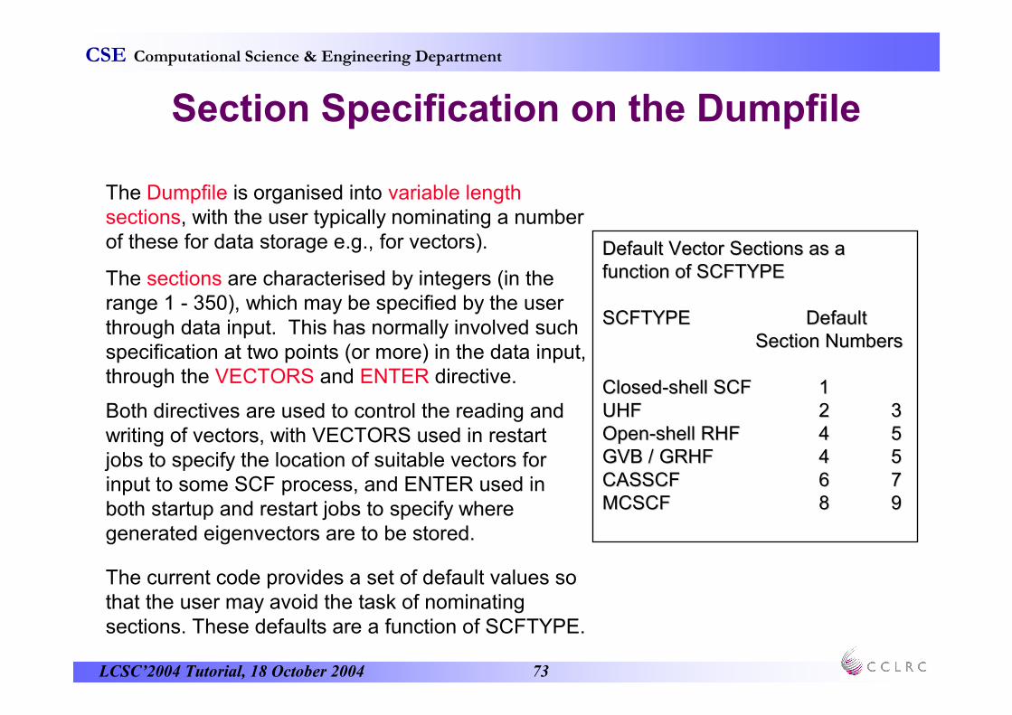
Section Specification on the Dumpfile
The Dumpfile is organised into variable length sections, with the user typically nominating a number of these for data storage e.g., for vectors).
The sections are characterised by integers (in the range 1 - 350), which may be specified by the user through data input. This has normally involved such specification at two points (or more) in the data input, through the VECTORS and ENTER directive.
Both directives are used to control the reading and writing of vectors, with VECTORS used in restart jobs to specify the location of suitable vectors for input to some SCF process, and ENTER used in both startup and restart jobs to specify where generated eigenvectors are to be stored.
The current code provides a set of default values so that the user may avoid the task of nominating sections. These defaults are a function of SCFTYPE.
Default Vector Sections as aDefault Vector Sections as a
function of SCFTYPEfunction of SCFTYPE
SCFTYPE SCFTYPE Default Default
Section NumbersSection Numbers
ClosedClosed--shell SCFshell SCF 11
UHFUHF 22 3 3
OpenOpen--shell RHFshell RHF 44 55
GVB / GRHFGVB / GRHF 44 55
CASSCFCASSCF 66 77
MCSCFMCSCF 88 99

LCSC’2004 Tutorial, 18 October 2004 74
CSE Computational Science & Engineering Department
environment variables
#!/bin/csh
setenv ed2 mfged2
setenv ed3 mfged3
../../bin/gamess << EOF
title
……
enter
EOF
file directive within dataset
#!/bin/csh
../../bin/gamess << EOF
file ed2 mfged2 keep
file ed3 mfged3 keep
title
…...
EOF
Routing of files
• By default files are deleted at the end of the job
• File specifications provide names and cause files to be retained
¤ set environment variable outside job
¤ use file directive
¤ Use -t, -k -r options to rungamess (described earlier)

LCSC’2004 Tutorial, 18 October 2004 75
CSE Computational Science & Engineering Department
Restarting Calculations
• Need to keep the Dumpfile
• Restart directive
¤ RESTART NEW
• provide new geometry
• load old vectors, hessian
¤ RESTART <task> .. As on runtypee.g. RESTART OPTIM
• calculation resumes the specified task, e.g. a geometry optimisation at the last stored geometry
¤ RESTART
• perform a new task but use the geometry as stored on the dumpfile
¤ RESTART <task> REGEN
• resume the task but regenerate all integral files
TITLE
H2CO - 3-21G DEFAULT BASIS
ZMATRIX ANGSTROM
C
O 1 1.203
H 1 1.099 2 121.8
H 1 1.099 2 121.8 3 180.0
END
ENTER
RestartRESTART
TITLE
H2CO+ - 2B2 - 3-21G DEFAULT BASIS - UHF
CHARGE 1
MULT 2
ZMATRIX ANGSTROM
C
O 1 1.203
H 1 1.099 2 121.8
H 1 1.099 2 121.8 3 180.0
END
SCFTYPE UHF
ENTER
restart1a.in
restart1b.in

LCSC’2004 Tutorial, 18 October 2004 76
CSE Computational Science & Engineering Department
Preparing GAMESS-UK input 1. Using Molden
• Z-matrices can be prepared using Molden
¤ Molden ⇒ ZMAT Editor
¤ Restrictions
• …...
• Can save z-matrix in GAMESS-UK form.
• Molden can also start simple interactive calculations
¤ Molden ⇒ ZMAT Editor ⇒ Submit Job

LCSC’2004 Tutorial, 18 October 2004 77
CSE Computational Science & Engineering Department
Visualisation and GAMESS-UK1. Molden
• Molden reads data from the GAMESS-UK output file
¤ read output (loads basis, vectors etc)
• Molden ⇒ read
¤ optimised structure
• Displayed by default
¤ calculating and display orbitals
• Molden ⇒ dens. Mode ⇒ orbital
¤ frequencies
• change the input to use RUNTYPE FORCE
• run the calculation, read the output
• Molden ⇒ Norm. Mode

LCSC’2004 Tutorial, 18 October 2004 78
CSE Computational Science & Engineering Department
Visualisation and GAMESS-UK 2. The CCP1GUI
• A free, extensible Graphical User Interface built around the Python open-source programming language and the VTK visualisation toolkit.
• Has the potential to run on all the major operating system platforms.
• Object-oriented design enables the rapid development of new interfaces to chemistry codes.
• Interfaces to GAMESS-UK, ChemShell and MOPAC.
• Support for a variety of molecular file formats including:
• Cartesian, Z-matrix, PDB, CHARMM, ChemShell, XMol, Gaussian and XML.

LCSC’2004 Tutorial, 18 October 2004 79
CSE Computational Science & Engineering Department
The GUI on Windows XP

LCSC’2004 Tutorial, 18 October 2004 80
CSE Computational Science & Engineering Department
Why was it developed?
• Many of the codes used within CCP1 would benefit from having a Graphical User Interface.
• Long-standing need for a graphical interface to GAMESS-UK.
• Particularly needed for for teaching purposes.
• Requirement for a simplified environment for constructing and viewing molecules.
• Need to be able to visualise the complex results of quantum mechanical calculations.
• Program should be free so no barriers to its widespread use.
• Need a single tool that can be made to to run on a variety of hardware/operating system platforms.
LCSC’2004 Tutorial, 18 October 2004 81
CSE Computational Science & Engineering Department
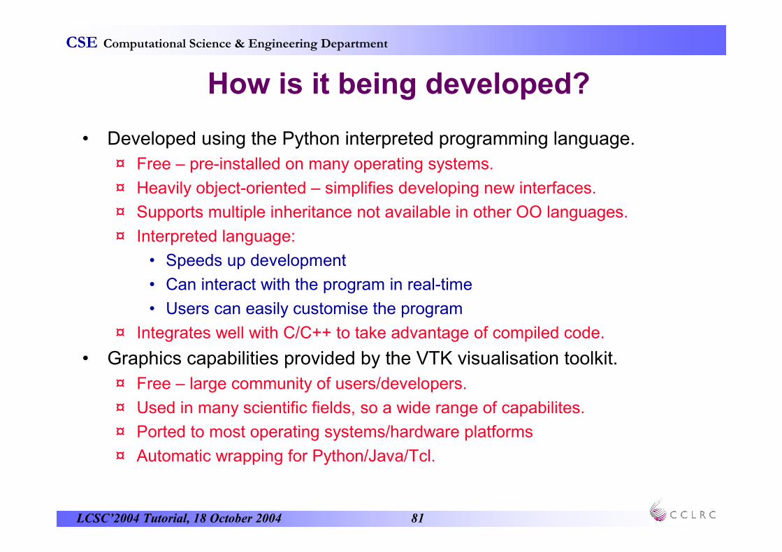
How is it being developed?
• Developed using the Python interpreted programming language.
¤ Free – pre-installed on many operating systems.
¤ Heavily object-oriented – simplifies developing new interfaces.
¤ Supports multiple inheritance not available in other OO languages.
¤ Interpreted language:
• Speeds up development
• Can interact with the program in real-time
• Users can easily customise the program
¤ Integrates well with C/C++ to take advantage of compiled code.
• Graphics capabilities provided by the VTK visualisation toolkit.
¤ Free – large community of users/developers.
¤ Used in many scientific fields, so a wide range of capabilites.
¤ Ported to most operating systems/hardware platforms
¤ Automatic wrapping for Python/Java/Tcl.

LCSC’2004 Tutorial, 18 October 2004 82
CSE Computational Science & Engineering Department
Current capabilities
• Interfaces to GAMESS-UK, ChemShell and MOPAC.
• Support for a variety of molecular file formats:
¤ Cartesian
¤ Internal Coordinates
¤ PDB
¤ Xmol, XML.
¤ CHARMM, ChemShell, Gaussian, GAMESS-UK.
• Powerful molecule builder.
• Variety of visualisation possibilities.

LCSC’2004 Tutorial, 18 October 2004 83
CSE Computational Science & Engineering Department
CCP1GUI Molecule Builder
Versatile molecule-constructing environment:
¤ Simple point-and-click operations for many functions.
¤ Commonly used molecular fragments added at the click of a button to quickly build up complex molecules.
¤ Highly-featured Z-matrix editor for Cartesian, internal and mixed coordinates
¤ Can convert between the different representations.
¤ Select and set the variables for a geometry optimisation.

LCSC’2004 Tutorial, 18 October 2004 84
CSE Computational Science & Engineering Department
Visualising Molecules
• Wireframe representation.
• “Ball and Stick” models.
• Contacts between non-bonded atoms.
• Extend repeat units.
• Can spend hours tweaking how things look…

LCSC’2004 Tutorial, 18 October 2004 85
CSE Computational Science & Engineering Department
Driving GAMESS-UK
• Set up and run most basic GAMESS-UK runtypes.
• Specification of the atomic basis sets.
• Control of SCF convergence.
• Set functional /grid / Coulomb fitting for DFT calculations.
• Calculate a variety of molecular properties.
• Control of Geometry optimisations/transition state searches.
• Specify where the job is run, which files are saved, etc.

LCSC’2004 Tutorial, 18 October 2004 86
CSE Computational Science & Engineering Department
Visualising Calculation Results I
• Animate vibrational frequencies.
• Create a movie from the steps in a geometry optimisation pathway.
• Visualise scalar data.
¤ Surfaces, grids, cut slices, volume rendering – can all be overlaid.
Transparent HOMO Volume-rendered charge density.
LCSC’2004 Tutorial, 18 October 2004 87
CSE Computational Science & Engineering Department
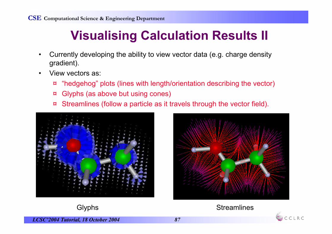
Visualising Calculation Results II
• Currently developing the ability to view vector data (e.g. charge density gradient).
• View vectors as:
¤ “hedgehog” plots (lines with length/orientation describing the vector)
¤ Glyphs (as above but using cones)
¤ Streamlines (follow a particle as it travels through the vector field).
Glyphs Streamlines

LCSC’2004 Tutorial, 18 October 2004 88
CSE Computational Science & Engineering Department
Impress your friends…
Electric field visualisations: TNT and Water

LCSC’2004 Tutorial, 18 October 2004 89
CSE Computational Science & Engineering Department
Future Developments
• Work underway to permit the GUI to query and download structuresstored in online XML databases as part of the eCCP1 project.
• As the data model progresses it will also become possible to store and retrieve the inputs and results of QM and MM calculations as XML.
http://www.e-science.clrc.ac.uk/web
• Develop interfaces to new QM and MM codes.
• Continue to expand the visualisation capabilities.
• Add new functionality – suggestions?…