the galaxy−dark matter connection - yale astronomy · outline • statistical description of...
TRANSCRIPT

The Galaxy−Dark Matter Connection
cosmology & galaxy formation with the CLF
Frank C. van den Bosch (MPIA)

Outline
• Statistical Description of Large Scale Structure
• Galaxy Bias & The Galaxy-Dark Matter Connection
• The Halo Model, Halo Bias & Halo Occupation Statistics
• The Conditional Luminosity Function (CLF)
• The Universal Relation between Light and Mass
• Constraining Cosmological Parameters with the CLF
• Halo Occupation Statistics from Galaxy Groups
• Constraining Galaxy Formation with Galaxy Ecology
• Conclusions

Correlation FunctionsDefine the dimensionless density perturbation field: δ(~x) = ρ(~x)−ρ
ρ
For a Gaussian random field , the one-point probability function is:
P (δ)dδ = 1√2πσ
exp[− δ2
2σ2
]dδ
〈δ〉 =∫
δP (δ)dδ = 0
〈δ2〉 =∫
δ2P (δ)dδ = σ2
Define n-point probability function : Pn (δ1, δ2, · · ·, δn) dδ1 dδ2 · · · dδn
Gravity induces correlations between δi so that
Pn (δ1, δ2, · · ·, δn) 6=n∏
i=1
P (δi)
Correlations are specified via n-point correlation function :
〈δ1δ2 · · · δn〉 =∫
δ1δ2 · · · δnPn (δ1, δ2, · · ·, δn) dδ1 dδ2 · · · dδn
In particular, we will often use the two-point correlation function
ξ(x) = 〈δ1δ2〉 with x = |~x1 − ~x2|

Galaxy BiasConsider the distribution of matter and galaxies, smoothed on some scale R
δ(~x) =ρ(~x) − ρ
ρδgal(~x) =
ngal(~x) − ngal
ngal
xxxxxxxxx Mass distribution xxxxxxxxx Galaxy distribution
ξ(r) = 〈δ(~x1)δ(~x2)〉 ξgal(r) = 〈δgal(~x1)δgal(~x2)〉
• There is no good reason why galaxies should trace mass .
• Ratio is galaxy bias: b(~x) = δgal(~x)/δ(~x)
• One can distinguish various types of bias:
linear, deterministic: δgal = b δ
non-linear, deterministic: δgal = b(δ) δ
stochastic: δgal 6= 〈δgal|δ〉• Real bias probably non-linear and stochastic
• Bias also depends on smoothing scale R
• Since δgal = δgal(L, M∗, ...) bias also depends on galaxy properties
δ gal
δ
Dekel & Lahav 1999

Handling Bias• Bias is an imprint of galaxy formation , which is poorly understood
• Consequently, little progress constraining cosmology wit h LSS
Q: How can we constrain and quantify galaxy bias in a convenient way?

Handling Bias• Bias is an imprint of galaxy formation , which is poorly understood
• Consequently, little progress constraining cosmology wit h LSS
Q: How can we constrain and quantify galaxy bias in a convenient way?
A: With Halo Model plus Halo Occupation Statistics!
The Halo Model describes CDM distribution in terms of halo building blocks ,under assumption that every CDM particle resides in virialized halo
• On small scales: δ(~x) reflects density distribution of haloes ( NFW profiles )
• On large scales: δ(~x) reflects spatial distribution of haloes ( halo bias )
PARADIGM: All galaxies live in Cold Dark Matter Haloes.
galaxy bias = halo bias + halo occupation statistics

Halo Model Ingredients
‘Halo Model View’‘Real View’
Coo
ray
& S
heth
(20
02)
Halo Density Distributions: (Navarro, Frenk & White 1997)
ρ(r) = ρs
(r/rs)(1+r/rs)2
Halo Mass Function: (Press & Schechter 1974)
n(m) =√
2π
ρm2
∣∣ d ln σd ln m
∣∣ √νe−ν/2
Halo Bias Function: (Kaiser 1994; Mo & White 1996)
b(m) ≡ δh(m)δ
= n(m|δ)−n(m)n(m) δ
= 1 + ν−1δsc
δsc is critical spherical collapse overdensity, σ2(m) is mass variance , and ν = δ2sc/σ2(m)

The Origin of Halo BiasDark Matter Haloes are a biased tracer of the dark matter mass distribution!
Modulation causes statistical bias of peaks (haloes)
Modulation growth causes dynamical enhancement of bias

Analytical Description of Halo Bias
Define halo bias as b(m) = δh(m)/δ
ffffff b(m) > 1 if m > m∗ (biased)
ffffff b(m) = 1 if m = m∗ (unbiased)
ffffff b(m) < 1 if m = m∗ (unbiased)
Halo bias has absolute minimim:
ffffff b > 1 − 1δsc
≃ 0.41
buf
Halo-Halo correlation function: for haloes of mass m
ξhh(r) ≡ 〈δh1δh2
〉 = b(m)2〈δ1δ2〉 = b(m)2ξ(r)

Halo Occupation StatisticsHow many galaxies, on average, per halo?
Halo Occupation Distribution: The HOD P (N |M) specifies the probabilitythat a halo of mass M contains N galaxies.
Of particular importance: first moment 〈N〉M =∞∑
N=0
N P (N |M)
How are galaxies distributed (spatially & kinematically) within halo?
Central Galaxy : located at center of dark matter halo.
Satellite Galaxies: nsat(r) ∝ ρdm(r) ⇐⇒ σsat(r) = σdm(r)
Supported by distribution of sub-haloes in N -body simulations
What are physical properties of galaxies (luminosity, color, morphology)
One needs separate HOD for each sub-class of galaxies...
Introduce Conditional Luminosity Function , Φ(L|M) , which expressesaverage number of galaxies with luminosity L that reside in halo of mass M

The Conditional Luminosity FunctionThe CLF Φ(L|M) is the direct link between halo mass function n(M) andthe galaxy luminosity function Φ(L):
Φ(L) =∫ ∞0
Φ(L|M) n(M) dM
The CLF contains a lot of important information, such as:
• halo occupation numbers as function of luminosity:
NM(L > L1) =∫ ∞
L1
Φ(L|M) dL
• The average relation between light and mass :
〈L〉(M) =∫ ∞0
Φ(L|M) L dL
• The bias of galaxies as function of luminosity:
ξgg(r|L) = b2(L) ξdm(r)
b(L) = 1Φ(L)
∫ ∞0
Φ(L|M) b(M) n(M) dM
CLF is ideal statistical ‘tool’ to investigate Galaxy-Dark Matter Connection

Luminosity & Correlation Functions
ccccc • 2dFGRS: More luminous galaxies are more strongly clustered.
ccccc • c ΛCDM: More massive haloes are more strongly clustered.
More luminous galaxies reside in more massive haloes
REMINDER: Correlation length r0 defined by ξ(r0) = 1

The CLF Model• The LFs of clusters are well fit by a Schechter function
• The LF of all field galaxies has a Schechter form
• The halo mass function has a Press-Schechter form
We therefore assume that the CLF also has the Schechter form:
Φ(L|M)dL = Φ∗
L∗
(L
L∗
)α
exp(−L/L∗) dL
Here Φ∗, L∗ and α all depend on M .
• Parameterize Φ∗, L∗ and α. In total our model has 8 free parameters
• Construct Monte-Carlo Markov Chain to sample posterior distribution offree parameters. (Neq = 104, Nstep = 4 × 10⁷, Nchain = 2000)
• Use MCMC to put confidence levels on derived quantities such as〈M/L〉(M) and α(M).
• Use MCMC to explore degeneracies and correlations between variousparameters.

The Relation between Light & Mass
vdB, Yang, Mo & Norberg, 2005, MNRAS, 356, 1233

Cosmological Constraints
vdB, Mo & Yang, 2003, MNRAS, 345, 923
See also Tinker et al. 2005; Vale & Ostriker 2005

HODs from Galaxy Groups
Halo Occupation Statistics can also be obtained directly from galaxy groups
Potential Problems: interlopers, (in)completeness, mass estimates
We developed new, iterative group finder, using an adaptive fi lter modeledafter halo virial properties Yang, Mo, vdB, Jing 2005, MNRAS, 356, 1293
• Calibrated & Optimized with Mock Galaxy Redshift Surveys
• Low interloper fraction ( <∼ 20%).
• High completeness of members ( >∼ 90%).
• Masses estimated from group luminosities.More accurate than using velocity dispersion of members.
• Can also detect “groups” with single member⊲ Large dynamic range ( 11.5 <∼ log[M ] <∼ 15).
Group finder has been applied to both the 2dFGRS (completed survey) and tothe SDSS (DR2, NYU-VAGC; Blanton et al. 2005)

The Relation between Light & Mass
YMBJ = Yang, Mo, vdB & Jing, 2005 vdB et al. 2006, in prep.
M05 = Mandelbaum et al. 2005

Galaxy EcologyMany studies have investigated relation between various galaxy properties(morphology / SFR / colour) and environment
(e.g., Dressler 1980; Balogh et al. 2004; Goto et al. 2003; Ho gg et al. 2004)
Environment estimated using galaxy overdensity (projected) to nth nearestneighbour, Σn or using fixed, metric aperture, ΣR.
• Fraction of early types increases with density
• There is a characteristic density (∼ group-scale) below whichenvironment dependence vanishes
• Groups and Clusters reveal radial dependence :late type fraction increases with radius
• No radial dependence in groups with M <∼ 1013.5h−1 M⊙
Danger: Physical meaning of Σn and ΣR depends on environment.
Physically more meaningful to investigate halo mass dependence of galaxyproperties. This requires galaxy group catalogues .
Important: Separate luminosity dependence from halo mass dependence .

Defining Galaxy Types
Data from NYU-VAGC (Blanton et al. 2005): SSFRs from Kauffma nn et al. (2003) and Brinchmann et al. (2004)

Halo Mass Dependence
The fractions of early and late type galaxies depend strongly on halo mass.
At fixed halo mass, there is virtually no luminosity dependence .
The mass dependence is smooth: there is no characteristic mass scale
The intermediate type fraction is independent of luminosity and mass.
(Weinmann, vdB, Yang & Mo, 2006)

Comparison with Semi-Analytical ModelComparison of Group Occupation Statistics with Semi-Analytical Model ofCroton et al. 2006 . Includes ‘radio-mode’ AGN feedback.
• SAM matches global statistics of SDSS
• Luminosity function, bimodal color distribution, and over all blue fraction
• But what about statistics as function of halo mass?

Constraining Star Formation TruncationTo allow for fair comparison, we run our Group Finder over SAM.
Wei
nman
n et
al.
(ast
ro−
ph/0
6064
58)
Satellites: red fraction too large: ⊲ strangulation too efficient as modelled
Centrals: fblue(L|M) wrong: ⊲ AGN feedback /dust modelling wrong
fblue(L, M) useful to constrain SF truncation mechanism

Conclusions
Galaxy Bias = Halo Bias + Halo Occupation Statistics
Halo Occupation Statistics can be modeled & constrained using:
• Halo Occupation Distribution (HOD) P (N |M)
• Conditional Luminosity Function (CLF) Φ(L|M)
or it can be ‘measured’ directly using galaxy groups
Halo Model and/or Halo Occupation Statistics can:
• Constrain Cosmological Parameters
• Constrain Galaxy Formation
In the near future we will be able to
• Constrain galaxy bias as function of redshift
• Obtain independent constraints from galaxy-galaxy lensin g

Constructing Mock Surveys• Run numerical simulations : ΛCDM concordance cosmology (WMAP1)
Lbox = 100h−1 Mpc and 300h−1 Mpc with 5123 CDM particles each.
• Identify dark matter haloes with ( FOF algorithm.
• Populate haloes with galaxies using CLF.
• Stack boxes to create virtual universe and mimick observations(magnitude limit, completeness, geometry, fiber collision s)
SGP
NGP
−1600 h Mpc
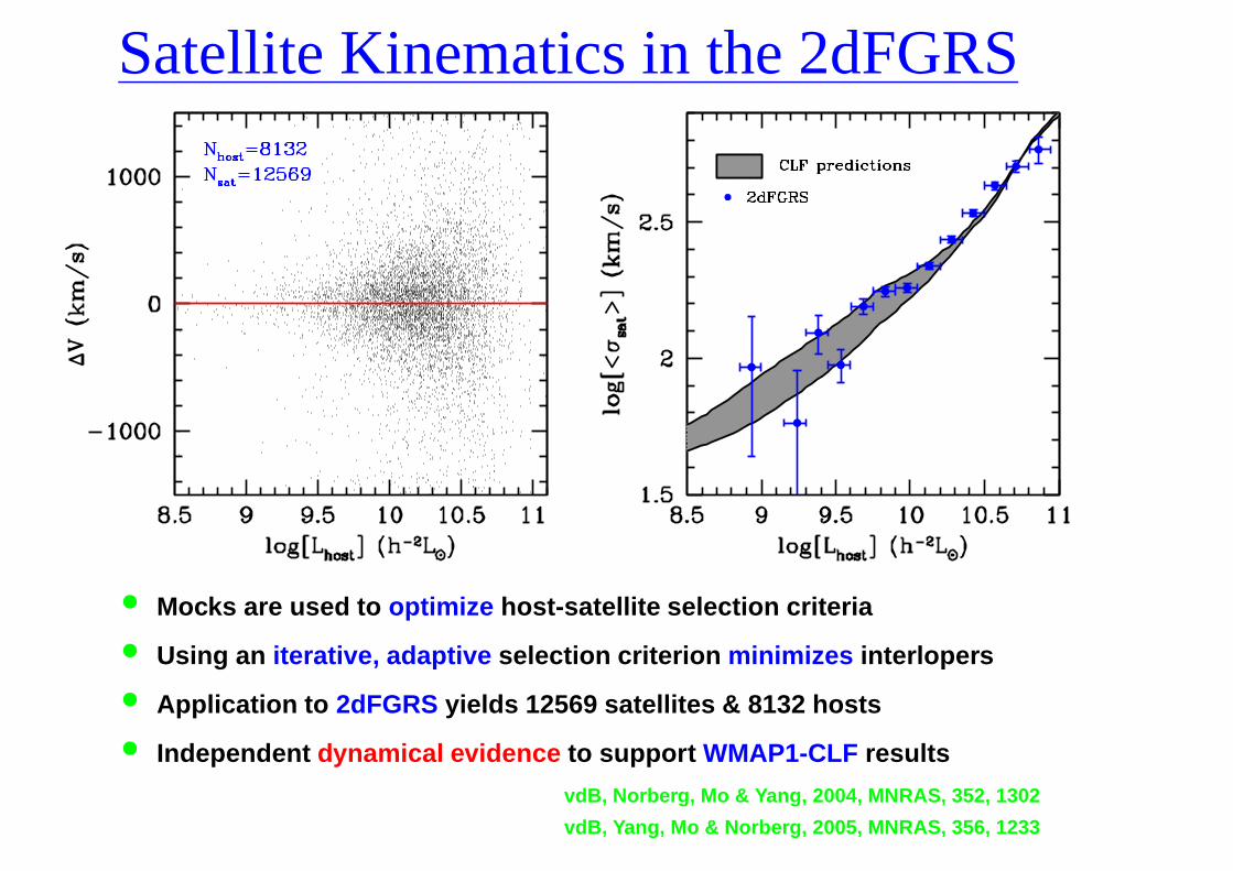
Satellite Kinematics in the 2dFGRS
• Mocks are used to optimize host-satellite selection criteria
• Using an iterative, adaptive selection criterion minimizes interlopers
• Application to 2dFGRS yields 12569 satellites & 8132 hosts
• Independent dynamical evidence to support WMAP1-CLF results
vdB, Norberg, Mo & Yang, 2004, MNRAS, 352, 1302
vdB, Yang, Mo & Norberg, 2005, MNRAS, 356, 1233

Problems for the WMAP3 Cosmology?
• In WMAP3 cosmology, haloes have lower mass-to-light ratios and areless concentrated.
• WMAP3-CLF underpredicts satellite velocity dispersions by ∼ 30%
• But, Lcen(M) in good agreement with group-data....
• Central galaxies do not reside at rest at center of halo.
vdB et al. 2006, in preparation

Brightest Halo Galaxies
Paradigm: Brightest Galaxy in halo resides at rest at center
In order to test this Central Galaxy Paradigm , we compare the velocity ofcentral galaxy to the average velocity of the satellites. De fine
R = Ns(vc−vs)σs
with vs = 1Ns
Ns∑i=1
vi and σs =
√1
Ns−1
Ns∑i=1
(vi − vs)2.
If Central Galaxy Paradigm is correct, P (R) follows a Student t-distributionwith Ns − 1 degrees of freedom
IMPORTANT: Applicability of this R-test depends strongly on abilityIMPORTANT: to find those galaxies that belong to same halo.
PROBLEM: Interlopers and incompleteness effects
SOLUTION: Use halo-based group finder and mock galaxy redshift surveys
DATA: Both 2dFGRS (Final Data Release) and SDSS (DR2, NYU-VAGC)

Evidence against Central Galaxy Paradigm
• We construct ten MGRSs , that only differ in the velocity bias (bvel) ofthe brightest halo galaxy
• The P (R) of 2dFGRS is best reproduced by MGRS with bvel = 0.5
• The null-hypothesis of the Central Galaxy Paradigm is ruled out atstrong confidence: PKS = 1.5 × 10⁻⁶
• Best-fit value of bvel = 0.5 suggests that specific kinetic energy ofcentral galaxies is ∼ 25% of that of satellites
vdB et al. 2005, MNRAS, 361, 1203

ImplicationsNon−Relaxed Galaxy Non−Relaxed Halo
• Brightest halo galaxy either oscillates in relaxed halo, or resides atpotential minimum of non-relaxed halo.
• Strong gravitational lensing (external shear?)
• Distortions in disk galaxies (lopsidedness & bars)
• Satellite kinematics σsat =√
1 + bvel σdm
with bvel = 〈|vcen|2〉/σsat

Large Scale Structure: TheoryGalaxy redshift surveys yield ξ(rp, π) with rp and π the pair separationsperpendicular and parallel to the line-of-sight.
redshift space CF: ξ(s) with s =√
r2p + π2
projected CF: wp(rp) =∞∫
−∞ξ(rp, π)dπ = 2
∞∫rp
ξ(r) r dr√r2−r2
p
Peculiar velocities cause ξ(rp, π)to be anisotropic.
Consequently, ξ(s) 6= ξ(r).
In particular, there are two effects:
• Large Scales: Infall (“Kaiser Effect”)
• Small Scales: “Finger-of-God-effect”

Large Scale Structure: The 2dFGRS
Peacock et al 2001
Hawkins et al 2001

Mock versus 2dFGRS: round 1
Yang, Mo, Jing, vdB & Chu, 2004, MNRAS, 350, 1153
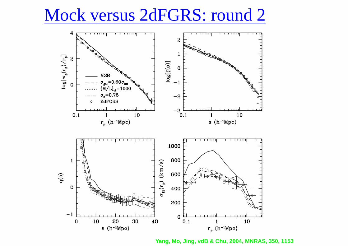
Mock versus 2dFGRS: round 2
Yang, Mo, Jing, vdB & Chu, 2004, MNRAS, 350, 1153

Large-Scale Environment DependenceInherent to CLF formalism is assumption that L depends only on M .
But Φ(L) has been shown to depend on large scale environment
Croton et al. 2005
Does this violate the implicit assumptions of the CLF formal ism?

Large-Scale Environment Dependence2dFGRSCLF
Populate haloes in N -body simulations with galaxies using Φ(L|M)
Compute Φ(L) as function of environment and type as in Croton et al. (2005)
Because n(M) depends on environment , we reproduce observed trend
There is no environment dependence, only halo-mass depende nce

Theoretical Expectations
From the fact that
δh(m) ≡ n(m|δ)n(m)
− 1 = b(m)δ
we obtain that
n(m|δ) = [1 + b(m)δ] n(m)
Since the halo bias b(m) is an increasing function of halo mass, theabundance of more massive haloes is more strongly boosted in overdenseregions than that of less massive haloes
In other words; massive haloes live in overdense regions
If more massive haloes host more luminous galaxies, we thus e xpect that theluminosity function of galaxies also depends on environmen t

Correlation FunctionsDefine the dimensionless density perturbation field: δ(~x) = ρ(~x)−ρ
ρ
For a Gaussian random field , the one-point probability function is:
P (δ)dδ = 1√2πσ
exp[− δ2
2σ2
]dδ
〈δ〉 =∫
δP (δ)dδ = 0
〈δ2〉 =∫
δ2P (δ)dδ = σ2
Define n-point probability function : Pn (δ1, δ2, · · ·, δn) dδ1 dδ2 · · · dδn
Gravity induces correlations between δi so that
Pn (δ1, δ2, · · ·, δn) 6=n∏
i=1
P (δi)
Correlations are specified via n-point correlation function :
〈δ1δ2 · · · δn〉 =∫
δ1δ2 · · · δnPn (δ1, δ2, · · ·, δn) dδ1 dδ2 · · · dδn
In particular, we will often use the two-point correlation function
ξ(x) = 〈δ1δ2〉 with x = |~x1 − ~x2|

Power SpectrumIt is useful to write δ(~x) as a Fourier series:
δ(~x) =∑~k
δ~kei~k·~x δ~k = 1V
∫δ(~x)e−i~k·~xd3~x
Note that δ~k are complex quantities: δ~k = |δ~k|eiθ~k
Decomposition in Fourier modes is preserved during linear evolution , so that
Pn
(δ~k1
, δ~k2, · · ·, δ~kn
)=
n∏i=1
P (δ~ki)
Thus, statistical properties of δ(~x) completely specified by P (δ~k)
A Gaussian random field is completely specified by first two moments:
〈δ~k〉 = 0
〈|δ~k|2〉 = P (k) Power Spectrum
〈δ~kδ~p〉 = 0 (for k 6= p)
The power spectrum is Fourier Transform of two-point correlation function:
ξ(r) = 1(2π)3
∫P (k)ei~k·~rd3~k = 1
2π2
∫ ∞0
P (k) sin krkr
k2dk

Mass Variance
Let δM(~x) be the density field δ(~x) smoothed (convolved) with a filter of
size Rf ∝ [M/ρ]1/3.
Since convolution is multiplication in Fourier space, we ha ve that
δM(~x) =∑~k
δ~k WM(~k) ei~k·~x
with WM(~k) the FT of the filter function WM(~x).
The mass variance is simply
σ2(M) = 〈δ2M〉 = 1
2π2
∫P (k)W 2
M(k) k2dk
Note that σ2(M) → 0 if M → ∞.

Press-Schechter FormalismIn CDM universes, density perturbations grow, turn around from Hu bbleexpansion, collapse, and virialize to form dark matter halo .
According to spherical collapse model the collapse occurs when
δlin = δsc ≃ 320
(12π)2/3 ≃ 1.686
δlin is linearly extrapolated density perturbation field
δsc is critical overdensity for spherical collapse.
Press-Schechter ansatz : if δlin,M(~x) > δsc then ~x is locatedPress-Schechter ansatz: in a halo with mass > M .
The probability that ~x is in a halo of mass > M therefore is
P (δlin,M > δsc) = 1√2πσ(M)
∞∫δsc
exp(− δ2
2σ2(M)
)dδ
The Halo Mass Function , then becomes
n(M)dM = ρM
dPdM
dM =√
2π
ρM2
∣∣ d ln σd ln M
∣∣ √νe−ν/2
where ν = δ2sc/σ2(M), and a ‘fudge-factor’ 2 has been added.

Galactic Conformity
Late type ‘centrals’ have preferentially late type satellites, and vice versa.
Satellite galaxies ‘adjust’ themselves to properties of their central galaxy
Galactic Conformity present over large ranges in luminosity and halo mass.
(Weinmann, vdB, Yang & Mo, 2006)

Luminosity Dependence
(Weinmann, vdB, Yang & Mo, 2005)

Mass-Luminosity Dependence
(Weinmann, vdB, Yang & Mo, 2005)

Radial Dependence
(Weinmann, vdB, Yang & Mo, 2005)

Dependence on Group-centric Radius
As noticed before, the late type fraction of satellites increases with radius.This trend is independent of halo mass !
Inconsistent with previous studies, but these included central galaxies.
Our results rule out group- and cluster-specific processes s uch asram-pressure stripping and harassment : nature rather than nurture !
(Weinmann, vdB, Yang & Mo, 2005)

Median Properties
(Weinmann, vdB, Yang & Mo, 2005)

Conditional Mass Funcion

Conditional Colour Funcion
(Weinmann, vdB, Yang & Mo, 2005)

Conditional Concentration Funcion
(Weinmann, vdB, Yang & Mo, 2005)

Blue Fraction as Function of LuminosityIn SAM virtually all satellites are red, contrary to SDSS, where the fraction ofred satellites decreases with luminosity.
In SAM, satellites stripped of hot gas halo immediately after accr etion
⊲ This strangulation is too efficient.

Blue Fraction as Function of Halo MassTo allow for fair comparison, we run our Group Finder over SAM.
Problem with central galaxies: At fixed halo mass, blue fraction increaseswith L in SAM, but decreases with L in SDSS.
⊲ Modelling of AGN feedback is not yet entirely correct

The Importance of Satellite Galaxies
Kinematics• Satellites sample large radii ⇒ virial mass estimator
• Only few satellites per halo ⇒ Need to stack many host/satellite pairs
• Beware of Interlopers & Observational Biases
Abundances
• Halo Occupation Numbers ⇔ Conditional Luminosity Function(Yang, Mo & van den Bosch 2003; van den Bosch, Yang & Mo 2003)
• Comparison with dark matter subhaloes(Moore et al. 1999; Klypin et al. 1999; Vale & Ostriker 2004; K ravtsov et al. 2004)
Radial Distribution
• Dark Matter Subhaloes show spatial anti-bias(Klypin et al. 1999; Ghigna et al. 2000; De Lucia et al. 2003; D iemand et al. 2004)
• Impact of tidal stripping, dynamical friction, harassment etc.(Moore et al. 1998; Mayer et al. 2001; Taffoni et al. 2003)

Selecting hosts & satellites
other galaxy in blue volume.At least f_h times brighter than any
In red volume and at leastf_s times fainter than host.
HOSTS
SATS
redshift
ProjectedDistance
All previous studies used very conservative selection criteria: fh = 2,
fs = 4, ∆Vh = ∆Vs = 1000 km s−1, Rh = 2h−1 Mpc, and
Rs = 0.5h−1 Mpc. (McKay et al. 2002; Brainerd & Specian 2003; Prada et al. 2003)
Use Mock Galaxy Redshift Surveys , constructed from CLF to test selectioncriteria.

Selecting hosts & satellites
N_h=1851N_s=3876
N_h=7863N_s=19099
N_s=16750N_h=10483
f_s=1.0
f_s=1.0R_h=2.0 chimpR_s=0.5 chimp
f_h=1.0
f_h=2.0
R_h=2.0 chimpR_s=0.5 chimpdV_h=1000 km/sdV_s=1000 km/s
f_s=4.0
f_h=1.0
dV_h=2000 km/sdV_s=2000 km/s
assume sigma(L)iterate

Measuring Satellite Kinematics

Interpreting Satellite Kinematics
Velocity dispersion of satellite galaxies follows from Jeans Equation :
σ2sat(r) = 1
nsat(r)
∫ ∞r
nsat(r′) ∂Φ
∂r(r′) dr′
The halo averaged expectation value:
〈σsat〉M = 4π〈Nsat〉M
∫ rvir
0nsat(r) σsat(r) r2 dr
Expectation value for the number of satellites follows from CLF:
〈Nsat〉M =∫ ∞
L1
Φ(L|M) dL − 1
Scatter in relation between M and host luminosity Lh:
〈σsat〉(Lh) =∫ ∞0
P (M |Lh)〈σsat〉MdM
Stacking host-satellite pairs yields satellite-weighted mean :
〈σsat〉(Lh) =R
∞
0P (M |Lh) 〈σsat〉M 〈Nsat〉M dMR
∞
0P (M |Lh) 〈Nsat〉M dM
Accouting for flux-limited surveys :
〈σsat〉(Lh) = 1V
∫ Ω
0dΩ
∫ zmax
0dz dV
dΩdz〈σsat(Lh, z)〉
You need CLF to properly interpret satellite kinematics
back

Various Statistics of Galaxy Groups
Yang, Mo, vdB & Jing 2005, MNRAS, 356, 1293
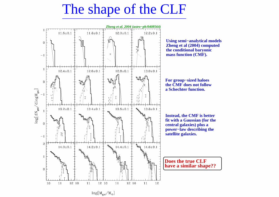
The shape of the CLF
Using semi−analytical modelsZheng et al (2004) computedthe conditional baryonicmass function (CMF).
For group−sized haloesthe CMF does not followa Schechter function.
Instead, the CMF is betterfit with a Gaussian (for thecentral galaxies) plus a power−law describing thesatellite galaxies.
have a similar shape??Does the true CLF
Zheng et al. 2004 (astro−ph/0408564)

Direct Determination of CLF from Groups
We determined CLFdirectly from groupsin 2dFGRS & mocks.
Group−sized haloeshave Schechter CLF.
Data is consistentwith Schechter CLF!
Mocks show similarbehavior, pointingto an artefact due to mass estimator.
Galaxy−sized haloesreveal Gaussianpeak of centralgalaxies.
Yang, Mo, Jing & vdB, 2005, MNRAS, 358, 217

Probing Clustering of Dark Matter Haloes
Yang, Mo, vdB & Jing 2005, MNRAS, 357, 608
• The group-group correlation function directly reflects the halo-halocorrelation function (no issues with galaxy bias)
• Promising tool to constrain cosmological parameters

Radial Distribution of Satellite Galaxies
Consistent with no spatial bias , but only if Rgal ≃ 15h−1 kpcL1/310

Concordance on Galactic Scales?Ωm = 0.25 ± 0.04 σ8 = 0.78 ± 0.06
Cosmologies with lower Ωm and lower σ8 yield dark matter haloes that aresignificantly less concentrated. This
• Alleviates problem with rotation curves of dwarf and LSB galaxies.
• Results in a TF zero-point that is ∼ 0.3 − 0.5 magnitudes brighter.

The Galaxy Phone Book
P (L, M) dL dM = 1ρL
n(M)Φ(L|M) L dL dM
P (M |L)dM = Φ(L|M) n(M) dMΦ(L)
50% of light is produced in haloes M <∼ 2 × 10¹²h−1 M⊙.

Luminosity & Correlation Functions
• On average, early-type galaxies are more luminous and more stronglyclustered than late-type galaxies.
• In general, more luminous galaxies are more strongly cluste red.
REMINDER: Correlation length r0 defined by ξ(r0) = 1

The Concordance CosmologyΩm = 0.3; ΩΛ = 0.7, h = 0.7, σ8 = 0.9, n = 1.0
vdB, Yang & Mo, 2003, MNRAS, 340, 771
Concordance model fits Φ(L) and r0(L) of both early- and late-type galaxies.

Semi-Analytical Models I
(Kauffmann et al. 1999)
Poor agreement with CLF; but SAM doesn’t fit LF

Semi-Analytical Models II
(Benson et al. 2002)
Good agreement with SAMs that fit LF

Bias in Satellite Kinematics
back

The Galaxy Correlation Function
The two-point galaxy-galaxy correlation function can be split in a1-halo and a 2-halo term
ξgg(r) = ξ1hgg(r) + ξ2h
gg (r) = ξ1hgg(r) + b2ξ2h
hh(r)
Here b and ξ2hhh(r) are computed as follows:
• b = 1ng
∫ ∞0
n(M) 〈N(M)〉 b(M) dM (Berlind & Weinberg 2002)
• 〈N(M)〉 =∫ L2
L1
Φ(L|M) dL
• ξ2hhh(r; M1, M2) = b(M1) b(M2) ξ2h
dm(r) (Mo & White 1996)
• ξ2hdm(r) = ξdm(r) − ξ1h
dm(r) (Ma & Fry 2000)
• ξdm(r) =∫ ∞0
∆2nl(k) sin(kr)
krdkk
NOTE: ξ1hgg(r) can be ignored at large r
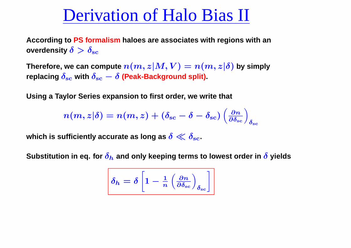
Derivation of Halo Bias IIAccording to PS formalism haloes are associates with regions with anoverdensity δ > δsc
Therefore, we can compute n(m, z|M, V ) = n(m, z|δ) by simplyreplacing δsc with δsc − δ (Peak-Background split) .
Using a Taylor Series expansion to first order, we write that
n(m, z|δ) = n(m, z) + (δsc − δ − δsc)(
∂n∂δsc
)
δsc
which is sufficiently accurate as long as δ ≪ δsc.
Substitution in eq. for δh and only keeping terms to lowest order in δ yields
δh = δ
[1 − 1
n
(∂n
∂δsc
)
δsc
]

Derivation of Halo Bias IIIAccording to the PS formalism the halo mass function is
n(m, z) =√
2π
ρm2 | d ln σ
d ln m|√νe−ν/2
with ν = ν(m, z) = δ2sc(z)/σ2(m)
If we define the halo bias as b(m, z) = δh/δ, one obtains that
b(m, z) = 1 + ν−1δsc
The characteristic mass m∗ is defined by σ(m∗) = δsc.
This implies that ν(m∗) = 1, and thus that b(m∗) = 1
ffffffffffffffffffff b(m, z) > 1 if m > m∗ (biased)
ffffffffffffffffffff b(m, z) = 1 if m = m∗ (unbiased)
fff 1 − 1δsc
< b(m, z) < 1 if m < m∗ (anti-biased)
Note that there is an absolute minimim to the halo bias.

Comparing 2dFGRS with SDSS
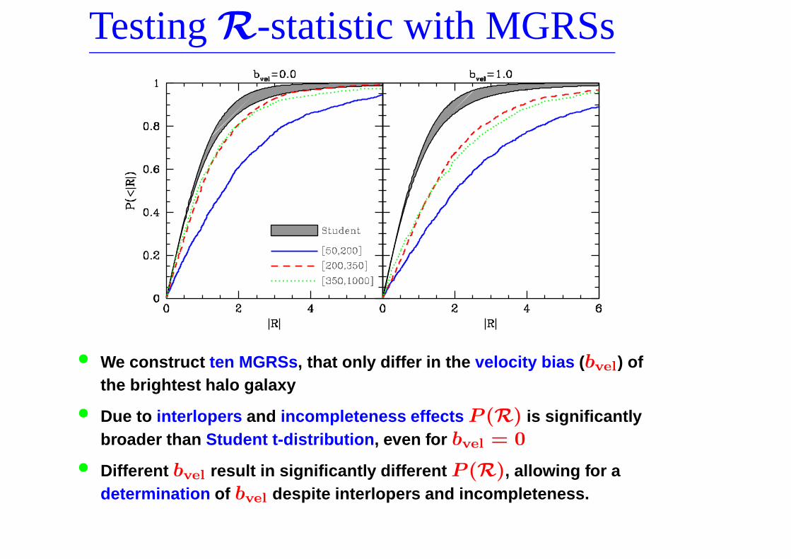
TestingR-statistic with MGRSs
• We construct ten MGRSs , that only differ in the velocity bias (bvel) ofthe brightest halo galaxy
• Due to interlopers and incompleteness effects P (R) is significantlybroader than Student t-distribution , even for bvel = 0
• Different bvel result in significantly different P (R), allowing for adetermination of bvel despite interlopers and incompleteness.

Mass Dependence ofbvel
The velocity bias bvel is larger for more massive haloes, in agreement with ahierarchical formation scenario .

Assumptions• All dark matter is collapsed into dark matter haloes
• All galaxies live in dark matter haloes
• Central galaxy resides at rest at center of halo
• Satellite galaxies follow dark matter distribition (NFW pr ofile)
• P (Nsat|M) is Poissonian
• Halo bias: b = b(M) ; HOD: P (N) = P (N |M)
• Accuracy of b(M), n(M), ρ(r) and ξdm(r)
• Halo is a cow, and therefore spherical
• What can we learn from HOD as function of redshift?

Assembly Bias: does it matter?
Assume that halo bias b = b(M, c) with c the halo concentration , but thatHOD does not depend on halo concentration, i.e., 〈N〉 = 〈N〉(M)
bg = 1ng
∫dM 〈N〉(M)
∫dc b(M, c) n(M, c)
However, when ignoring this assembly bias we compute
b′g = 1
ng
∫dM 〈N〉(M) b(M) n(M)
Since b(M) = 1n(M)
∫b(M, c)n(M, c)dc one has that
b′g = 1
ng
∫dM〈N〉(M)
∫dc b(M, c) n(M, c) = bg
However, when 〈N〉 = 〈N〉(M, c) this is no longer true, and b′g 6= bg
Important questions:
• What is b(M, c)?
• Do equal-mass haloes with different c have different galaxy properties?
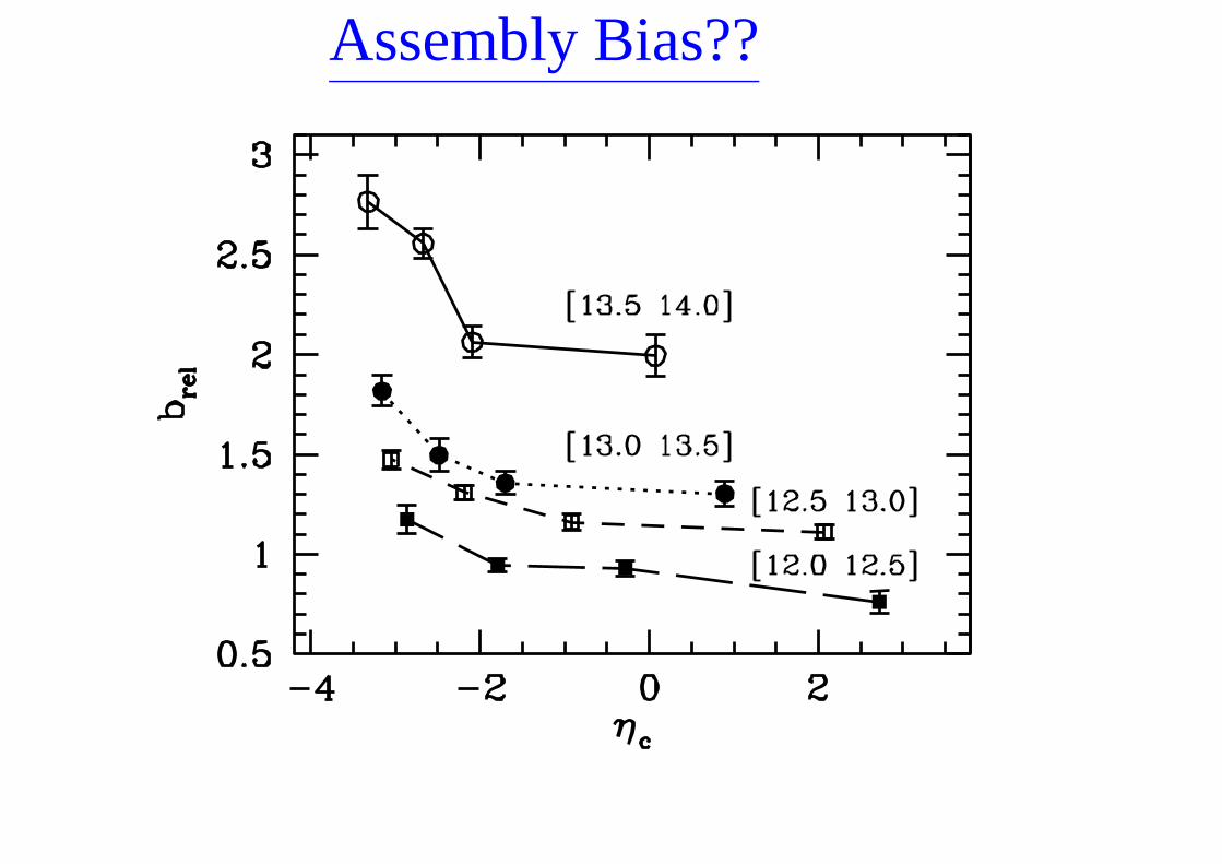
Assembly Bias??

Derivation of Halo Bias IDefine halo bias as b(m) = δh(m)/δ
Let N(m|M, V ) be the number of haloes of mass m in volume V .
The volume V has an overdensity δ so that M = V ρ(1 + δ) and initiallywas associated with a volume V0 = V (1 + δ).
The overdensity in the number of haloes of mass m is
δh(m) = N(m|M,V )n(m)V
− 1
Here n(m) is the (average) halo mass function.
To take account of the dynamical bias we write
N(m|M, V ) = n(m|M, V )V0 = n(m|M, V )V (1 + δ)
so that
δh(m) = n(m|M,V )n(m)
(1 + δ) − 1
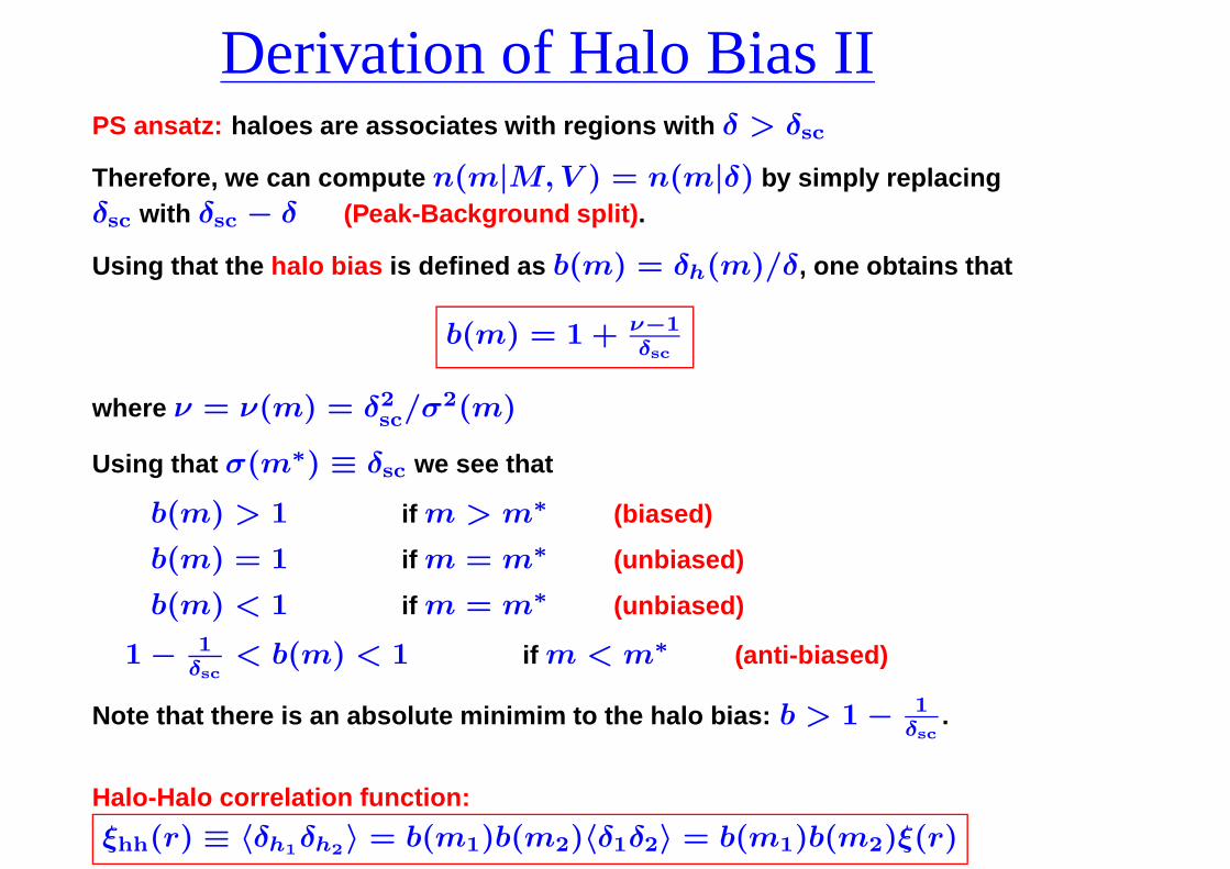
Derivation of Halo Bias IIPS ansatz: haloes are associates with regions with δ > δsc
Therefore, we can compute n(m|M, V ) = n(m|δ) by simply replacingδsc with δsc − δ (Peak-Background split) .
Using that the halo bias is defined as b(m) = δh(m)/δ, one obtains that
b(m) = 1 + ν−1δsc
where ν = ν(m) = δ2sc/σ2(m)
Using that σ(m∗) ≡ δsc we see that
ffffff b(m) > 1 if m > m∗ (biased)
ffffff b(m) = 1 if m = m∗ (unbiased)
ffffff b(m) < 1 if m = m∗ (unbiased)
fff 1 − 1δsc
< b(m) < 1 if m < m∗ (anti-biased)
Note that there is an absolute minimim to the halo bias: b > 1 − 1δsc
.
Halo-Halo correlation function:
ξhh(r) ≡ 〈δh1δh2
〉 = b(m1)b(m2)〈δ1δ2〉 = b(m1)b(m2)ξ(r)