the future of labor: automation and the labor share in the
TRANSCRIPT

The Future of Labor: Automation and the Labor
Share in the Second Machine Age*
Hong Cheng
Wuhan University
Lukasz A. Drozd
Federal Reserve Bank of Philadelphia
Rahul Giri
International Monetary Fund
Mathieu Taschereau-Dumouchel
Cornell University
Junjie Xia
Peking University
February 23, 2021
Abstract
We study the effect of modern automation on firm-level labor shares using a 2018 survey of 1,618
manufacturing firms in China. We exploit geographic and industry variation built into the design
of subsidies for automation paid under a vast government industrialization program, “Made In
China 2025,” to construct an instrument for automation investment. We use a canonical CES
framework of automation and develop a novel methodology to structurally estimate the elasticity
of substitution between labor and automation capital among automating firms, which for our
preferred specification is 3.8. We calibrate the model and show that the general equilibrium
implications of this elasticity are consistent with the aggregate trends during our sample period.
Key words: labor share, labor’s share in income, automation, labor demand, industrial robots.
JEL Classifications: D33, E25, O33, J23, J24, E24, O25.
*Preliminary, comments welcome. We thank Jonas Arias, Mark Bils, Julieta Caunedo, Jonathan Eaton, LoukasKarabarbounis, Samuel Kortum, Alex Monje-Naranjo, and Marina Mendes Tavares for their insightful comments. Weare particularly grateful to Jonas Arias for his technical insights. All remaining errors are ours. The views expressed inthis paper are solely those of the authors and do not necessarily reflect those of the International Monetary Fund, theFederal Reserve Bank of Philadelphia or the Federal Reserve System. Cheng: [email protected]; Drozd (correspond-ing author): [email protected], Federal Reserve Bank of Philadelphia Ten Independence Mall Philadelphia,PA 19106-1574; Giri: [email protected]; Taschereau-Dumouchel: [email protected]; Xia: [email protected].
1

The share of labor in national income has been shrinking globally since the early 1980s, under-
mining economists’ confidence that a constant labor share is an immutable fact of growth as famously
postulated by Kaldor (1961). Karabarbounis and Neiman (2013) measure that decline in multiple
countries and find that the labor share has fallen by about five percentage points since then—a large
movement by historical standards.1 One hypothesis is that this decline is driven by a modern wave
of automation that erodes humans’ advantage in both routine and, more recently, non-routine cog-
nitive tasks. According to this hypothesis, increasingly sophisticated “robots”—fueled by advances
in artificial intelligence, machine learning and dexterous automation—are now eating into labor’s
share of national income. A growing number of studies seem to confirm that technology is indeed
rapidly changing how capital can be substituted for labor.2 But while these developments might
have captured the imagination of intellectuals, popular writers and politicians, concrete evidence
for how modern automation is affecting the labor share is scant in the economic literature.3 This
paper contributes to the measurement and understanding of automation’s impact on labor’s share in
income on firm and industry level.
Measuring the effect of modern automation on the labor share is a challenging task because
investment in automation is oftentimes driven by unrelated trends or shocks that are difficult to
measure and distinguish from the causal effect of automation. For example, demand shocks that
increase markups—and thereby lower the labor share of a firm or an entire industry—may push
firms to expand production and invest in automation to satisfy rising demand for their products, in
effect creating a non-causal link between the labor share and automation. An analogous effect can
be driven by other shocks when a firm’s demand features a nonconstant elasticity. More importantly,
offshoring of labor intensive activities to lower income countries may push existing firms to specialize
in goods that are more capital intensive, having a similar effect.4 To address such or similar concerns,
a careful identification strategy is required to determine whether the link between automation and
1See Dao et al. (2017) for updated evidence. See also Autor et al. (2003), Goos and Manning (2007), Acemogluand Autor (2011), David and Dorn (2013), Michaels et al. (2014) and Dvorkin and Monge-Naranjo (2019) for evidenceon how automation is impacting jobs and job polarization.
2For example, according to Manyika et al. (2019), a quarter of labor hours is estimated to be lost to automation by2030, with highly skilled occupations expected to be at stake as much as low skilled occupations. Similarly, Muro et al.(2019) estimate that “approximately 25% of U.S. employment will face high exposure to automation in the comingdecades—with greater than 70% of current task content at risk of substitution.” See also Frey and Osborne (2017).For a contrarian view, see the work by Arntz et al. (2016). While their estimates are considerably smaller, they arenonetheless sizable.
3See, for example, Brynjolfsson and McAfee (2014), Ford (2009) or Frey (2020).4In a similar vein, Hubmer (2020) shows that changing consumption patterns may partly account for the decline
in the labor share in the US.
2

labor share is indeed a technological one.
In this paper, we attack this problem by developing a novel approach that uses policy-induced
local variation in the price of automation capital as an instrument for automation investment at
the firm level. To implement our approach, we use new data from a survey of 1,618 Chinese manu-
facturing firms conducted by the Wuhan University Institute of Quality Development Strategy and
designed in collaboration with a number of researchers from the Hong Kong University of Science and
Technology, Stanford University and the Chinese Academy of Social Sciences.5 Our data provides
detailed information on firms’ operations between 2015 and 2017, including the type of equipment
they purchased and, most importantly, the subsidies that they received from the government for
the purchases of automation capital (industrial robots and numerically controlled machines). These
subsidies were paid under an unprecedented government industrialization program, “Made in China”
(MIC, hereafter), and they were implemented by local municipalities. As a result, subsidy rates
varied considerably across cities and industries. Here we exploit this variation in the effective price
of automation capital to identify the causal impact of automation on the labor share.
To develop our empirical strategy, we extend a canonical model of automation—along the lines
of Graetz and Michaels (2018) and Acemoglu and Restrepo (2018)—and lay out how, in that theory,
after adding a large amount of firm- and industry-level heterogeneity in parameters and shocks, the
presence of orthogonal variation in subsidies for automation capital can identify the causal impact
of automation on the labor share. We state the assumptions under which this identification scheme
is valid, and discuss its validity and limitations in the context of our analysis. We then show how to
structurally estimate the key parameter responsible for that relationship in the model: the elasticity
of substitution between labor and automation capital. While we use this analysis in the context of a
particular dataset, our approach is general and can be applied to identify the impact of automation
on the labor share whenever (exogenous) variation in prices is available.
Substantively, we find that the firm-level elasticity of substitution between automation capital and
labor falls between 3 and 4.5 across different empirical specifications. Our preferred point estimate is
3.8. The fact that this elasticity is significantly larger than 1 indicates that automation capital and
labor are strong substitutes among actively automating firms, and so cheaper automation technologies
5China is a good case to study the impact of automation as it has been one of the most aggressive adopters ofrobots in the world in the past decade. The staggering pace of robot adoption in China is evident from the fact thatChina’s share in the global market for robots went from 3.7 percent in 2005 to around 30 percent in 2016. China’sMIC aims to raise the global market share of Chinese-made robots to over 50 percent by 2020. At the same time,China’s robot density was below the global average, with only 68 units per 10,000 workers in 2016, compared to theUS stock of almost 200. Source: International Federation of Robotics (World Robotics Reports), Statista.com.
3

do have a large negative impact on the labor share of income at the firm level.
We provide an assessment of whether this fairly high elasticity is consistent with the aggregate
trends in our dataset and with the overall Chinese economy during this time period. To do so, we
calibrate our model to match key moments characterizing our sample, such as the growth of value
added among automation firms, the growth in the stock of automation capital, the growth of wages,
etc. We find that the firm-level microeconomic elasticity of substitution between automation and
labor that we estimate is consistent with the observed decline in the aggregate labor share. Moreover,
we show that a lower elasticity would counterfactually imply too much growth in the value added
of automating firms relative to the industry average. We also find that the aggregate impact of
automation ultimately depends on how spread out automation is across firms, which we refer to as
the extensive margin of automation.
Finally, while our analysis pertains to Chinese data, the well-documented decades-long trend of
the declining quality-adjusted price of automation equipment sheds light on the declining labor share
in the U.S. manufacturing sector during the last several decades—which fell from an average of .61
to .41 between 1960 and the 2000s.6
Related literature. Our paper is one of a few that estimate the causal impact of modern au-
tomation on the labor share. The most closely related studies are Acemoglu and Restrepo (2020)
and Graetz and Michaels (2018). Both papers use different variants of a shift-share type of identi-
fication and do not focus on the labor share. The effects they measure capture general equilibrium
adjustments that may take place due to changes in prices and factor mobility over the long-run. In
contrast, our identification focuses on micro-level elasticities that are embedded in the production
technologies. Both approaches have their strengths, with ours being particularly useful as an input
into modeling.7
6See Kehrig and Vincent (2018) for a comprehensive analysis of the trends in the U.S. manufacturing sector, whichthese numbers are taken from. While their analysis does not explicitly relate observed changes to automation, it doeseliminate several other possibilities. Developed countries were ahead of China in terms of automation by at least adecade as of 2015, but since then Chinese automation has progressed at an extremely rapid pace. For quality-adjustedseries of the price of industrial robots, see Graetz and Michaels (2018) (Figure 1). Their evidence points to a declinebetween 1990 and 2004 by a factor of five (based on 1990 dollars). For comparison, nominal wages grew on average105 percent in the six reported countries. We are not aware of more recent quality-adjusted series but nonadjustedseries are available from various industry sources.
7It is important to note that the shift-share identification does not automatically remove all the effects of offshoringwhen its reach is global. Import competition from low-wage countries such as China (or within NAFTA) might haveled firms in developed countries to shift focus to capital-intensive products, and this, rather than the adoption ofnew automation technology might have reduced employment and wages in the exposed sectors, occupations or areas.Acemoglu and Restrepo (2020) discuss this issue and devise supplementary ways of addressing it. They point to the factthat automation and import competition are not as strongly correlated. While this is an important piece of evidence,
4

The paper by Autor and Salomons (2018) is also related to our work due to its focus on the link
between the labor share and productivity growth. It does not, however, provide causal identification
of the impact of automation. Finally, in a related and complementary work to ours, Humlum (2019)
provides a comprehensive analysis of robot adoption in Denmark and the distributional impact of
robots on employment.8
The rest of the paper is organized as follows. Section 1 discusses the theory of automation that
we use to develop our identification strategy. Section 2 discusses the data and our empirical strategy,
and presents the results. Section 3 discusses the aggregate implications of our calibrated model and
provides robustness analysis of our estimation procedure using model-generated data.
1 Model
We start by laying out the theory that forms the basis for both our empirical and quantitative
analysis. Our model is fairly standard and links the quality-adjusted price of automation capital to
automation investment and the labor share.
1.1 Environment
Time is discrete and the horizon is infinite. There are n cities indexed by c ∈ 1, 2, . . . , n
and m industries indexed by i ∈ 1, 2, . . . ,m. For convenience, we refer to the tuple (c, i) as an
island. Islands are populated by a continuum of firms of a fixed measure Ωci > 0, each producing
a differentiated good that is aggregated into a composite homogenous consumption good sold at
home and abroad at a unitary (global) price. Firms and goods are indexed by a unique identifier
ω ∈ Ωci ⊂ R, and we denote by c (ω) and i (ω) the city and industry of firm/good ω. There
is an economy-wide labor market such that the wage rate is common to all firms. The economy is
sufficiently small to take world prices as given and so the cost of funds is exogenous. To model shocks
to firm-level markups—a major concern in the measurement of the causal link between automation
and the labor share—we assume that a firm ω operates in one of k distinct markets, indexed by
j ∈ 1, 2, . . . , k, on each island. The transition between these markets follows a Markov process
such weak correlation may arise if import competition affects more the sectors that do not have the opportunity tospecialize in goods that are automation capital intensive. Such sectors, occupations or areas would then suffer themost from import competition, while those that can specialize in capital intensive goods would look less exposed. Ourpaper complements their analysis by providing additional evidence for the effect of automation.
8The work by Ciminelli et al. (2018) studies the link between the labor share declines with the efficacy of thereallocation of labor across countries.
5

independent of any firm or island characteristic, and the law of large numbers yields constant shares
of firms in each market. We denote by Ωcij ⊂ Ωci the set of firms on island (c, i) that operate in
market j. This structure allows us to demonstrate the robustness of our estimation procedure to the
presence of such shocks.
Demand structure and aggregation
Goods are aggregated by two layers of competitive sectors: the final good sector and the interme-
diate good sector. On each island, the outputs of individual firms are combined into the production
of an island-specific composite good and the island-specific composites are then again aggregated
into a homogenous final good that is sold globally at a normalized (numeraire) price P = 1—with
the goods market clearing condition dropped to reflect this assumption.
The final good producers convert a vector of differentiated island composite goods Qci into Y
units of final goods according to the production function
Y =
(n∑c=1
m∑i=1
D1ρ
ciQci
ρ−1ρ
) ρρ−1
, (1)
where Dci are fixed weights such that∑
ciDci = 1, and ρ > 0 is the elasticity of substitution between
goods. Final good producers take prices as given and maximize static profits given by
maxY,Qci
P (t)Y −n∑c=1
m∑i=1
Pci (t)Qci,
where Pci is the price of the composite good from industry i in city c, and where Y is given by the
production function (1). The resulting demand function for the composite good from island i is
Qci (t) = Dci
(Pci (t)
P (t)
)−ρY,
and the normalization of the price of the final good implies
P (t) =
(n∑c=1
m∑i=1
DciPci (t)1−ρ
) 11−ρ
≡ 1.
At the island level, a sector of competitive producers aggregates goods of all firms from all
markets on the island into a composite bundle Qci sold to the final good sector at a unit price Pci.
6

The producers solve
maxq(ω)
Pci (t)Qci −k∑j=1
∫Ωcij
p (t, ω) q (t, ω) dω,
where p (t, ω) and q (t, ω) denote the price and quantity of good ω, respectively. That industry uses
the production technology
Qci =k∏j=1
(∫Ωcij
d (t, ω)1θj q (t, ω)
θj−1
θj dω
)φjθjθj−1
.
The terms d (t, ω) are time-varying demand shocks affecting each individual firm and that follow an
arbitrary process. The parameter θj > 0 is the elasticity of substitution across goods in market j,
and φj is the intensity of market j. We impose constant returns to scale on the production function
and so∑m
j=1 φj = 1. By the zero profit condition, equilibrium prices satisfy
Pci (t) =∏j
(Pcij (t)
φj
)φj
,
and the price index for market j in city c in industry i at time t is
Pcij (t) =
(∫Ωcij
d (t, ω) p (t, ω)1−θj dω
) 11−θj
.
The demand curve for products produced by firm ω on island (c, i) and operating in market j(t, ω)
is given by
q (t, ω) = d (t, ω)
(p (t, ω)
Pcij(t,ω) (t)
)−θj(t,ω) ( Pci (t)
Pcij(t,ω) (t)
)φj(t,ω)Qci (t) . (2)
Notice that the market j (t, ω) the firm operates in, and which changes stochastically over time, shifts
the overall demand for its goods (through φj) and the elasticity of that demand is θj.
7

Production technology
The production technology of a firm combines support capital ks, equipment ke, automation
capital m, support labor ls and production labor l, and it is summarized by the production function9
Fω (ks, ls, ke, l,m) = A (t, ω)(kγωs l
1−γωs
)ηω (a
1σωω
(kαωe l1−αω
)σω−1σω + (1− aω)
1σω m
σω−1σω
)(1−ηω) σωσω−1
. (3)
The block kγωs l1−γωs corresponds to activities (tasks) in support of production activities, which are
captured by the last term in parentheses. For instance, support capital ks might include buildings
and structures; support labor ls could include management, sales force, or any support employees
that assist production activities but whose employment is only indirectly affected by automation.
These inputs are aggregated in a Cobb-Douglas fashion. The parameter 0 ≤ γω ≤ 1 determines the
intensity of capital and the parameter 0 ≤ ηω ≤ 1 determines how intensive the firm is in support
and productive activities. A (t, ω) is time-varying total factor productivity.
The second block of the production function (between the large parentheses) describes production
activities. These activities can be completed by a mix of equipment ke and production labor l, also
combined in a Cobb-Douglas fashion, or by using labor-saving automation capital m. The first
option captures traditional techniques for completing production activities and is characterized by a
price-invariant labor share determined by the parameter 0 ≤ αω ≤ 1. The second option captures
automation and involves no labor. The elasticity of substitution σω > 0 links the two terms and
determines how easy it is to automate activities that would traditionally be produced using an
equipment-labor mix. The parameter 0 ≤ aω ≤ 1 describes how intensive the production function is
in automation capital.
We use the parameter aω to distinguish between the intensive and extensive margins of automation
investment. The intensive margin refers to the accumulation of automation capital m by firms that
are able to use that equipment in production (aω < 1). In contrast, the extensive margin of adoption—
the spread of automation across firms—is determined by the distinction between firms that can use
automation (aω < 1) and those that cannot (aω = 1).
The parameters of the production function in (3) are indexed by ω and they may vary across
firms. We allow the distributions of these parameters to be arbitrary at this point, although the
calibration of the model imposes more structure on how parameters are distributed.
9The production function pertains to the firm’s value added and does not involve intermediate goods.
8

To gain intuition about the notion of automation conveyed by the production function (3), consider
a simple task that involves nailing two pieces of material together. This task can be done by a
worker (production labor l) who uses a hammer (equipment ke) or, alternatively, by an autonomous
hammering robot (automation capital m) that performs the task on its own. The elasticity of
substitution σω then describes how easy it is for the firm to substitute production labor by automated
machinery with any such “automatable” task. Finally, whoever does the hammering (worker or robot)
might need a building (support capital ks) as a place to work and a manager (support labor ls) to
supervise production, which is captured by the term in front of the bracket.
Acemoglu and Restrepo (2020) microfound this interpretation of the above production function
using a task-based model. In their theory, the parameter aω maps onto the number of tasks for
which automation technology has been developed to date (automatable tasks), and the elasticity of
substitution σω maps onto the parameters pertaining to the task-level production function, which
determines how much labor and capital the firm chooses per automatable task, given prices.
A notable feature of the above production function is that it is consistent with the Kaldor (1961)
fact that the labor share remained constant for several decades. Indeed, if automation capital is
impossible to obtain (infinite price for m), (3) collapses to a standard Cobb-Douglas aggregator with
a constant labor share equal to
LSO (t, ω) :=
θj(t,ω) − 1
θj(t,ω)
(1− ηω) (1− αω)︸ ︷︷ ︸LSOP
+θj(t,ω) − 1
θj(t,ω)
ηω (1− γω)︸ ︷︷ ︸LSON
. (4)
But once the first automation technologies start to become available, firms might begin using them
in production, in which case the labor share LS (t, ω) will move away from its initial LSO (t, ω)
value. For later use, we refer to LSO as the automation-free labor share, LSOP as the automation-
free labor share in production activities and LSON as the automation-free labor share in support
(nonproduction) activities. By construction, automation only affects labor share via production
activities pertinent to LSOP .
Firm problem
We denote the equilibrium wage rate by w. The user costs associated with the three forms of
capital available to the firm are assumed to be determined by a fixed global cost of funds r, the
price of each type of capital and their corresponding depreciation rates. We denote the user cost
9

of structures by rs (t), the user cost of equipment by re (t), and the user cost of automation by
rm (t) (1− s (t, ω)), where s (t, ω) captures any policy-induced time-varying changes in the user cost
of automation capital that may vary across firms. Note that s (t, ω) can vary across firms and across
time. Later on, we will map s (t, ω) to government subsidies for automation investment that we
observe in the data and use it to develop our identification strategy.
The user costs of capital are implied by our assumptions of fixed global cost of funds r, the
assumption of linear depreciation of capital, and a fixed relative price of each type of capital good in
terms of the global final good (which is the numeraire). For instance, if we denote by pm the price of
one unit of automation capital, then we can write
pm (t) (1− s (t, ω)) (1 + r)︸ ︷︷ ︸cost of funds for purchase
− (1− δm) pm (t+ 1) (1− s (t, ω))︸ ︷︷ ︸value of undepreciated capital
= rm (t) (1− s (t, ω)) , (5)
where δm is the depreciation rate of automation capital and
rm (t) := pm (t) (1 + r)− (1− δm) pm (t+ 1) . (6)
is the user cost of automation capital before subsidies. The formula assumes that the subsidy affects
the cost of replacing undepreciated capital (1− δm) pm, which makes sense in the context of our
data since the duration of “Made in China 2025” is about a decade and the estimated lifetime of
automation equipment and robots is also about a decade. Under this assumption an increase in the
subsidy rate s and a decline in the price of capital pm are equivalent. User costs of other forms of
capital are defined analogously to (6).
The problem of the firm boils down to a static profit maximization problem of the form
π (t, ω) := maxq
(p (t, ω)− λ (t, ω)) q, (7)
where the price p (t, ω) satisfies the demand equation (2) and λ (t, ω) is the marginal cost of produc-
tion, which is defined by the cost minimization problem of the form
λ (t, ω) := minl,ke,ks,m
rs (t) ks + re (t) ke + rm (t) (1− s (t, ω))m+ w (t) (ls + l) , (8)
subject to Fi (ks, ls, ke, l,m) ≥ 1. It is straightforward to show that a standard constant markup
10

pricing rule applies here as long as each firm is atomistic, and so
p (t, ω) =θj(t,ω)
θj(t,ω) − 1λ (t, ω) , (9)
where j(t, ω) is the market in which firm ω currently operates.10 As expected, a change in market j
is akin to a markup shock. The lemma below characterizes the marginal cost of production λ (t, ω)
as a function of prices and parameters.
Lemma 1. The marginal cost of production λ (t, ω) is given by
λ (t, ω) =1
A (t, ω)
(λs (t, ω)
ηω
)ηω (aωλe (t, ω)1−σω + (1− aω) (λm (t, ω))1−σω) 11−σω
1− ηω
1−ηω
, (10)
where
λs (t, ω) =
(rs (t)
γω
)γi ( w (t)
1− γω
)1−γω, λe (t, ω) =
(re (t)
αi
)αω ( w (t)
1− αω
)1−αω, λm (t, ω) = rm (t) (1− s (t, ω)) .
Proof. All proofs are in Appendix C.
The effect of the price of automation on the marginal cost is captured by the last term in between
the large parentheses in (10) and it depends on the price of automation capital and the elasticity of
substitution between automation capital and labor σω.
Total labor supply in the economy is fixed and the wage rate w is determined by the usual
economy-wide market clearing. The assumption of a global market for a homogeneous final good and
common interest rate r eliminates the need for an explicit statement of the household problem and
we omit it. The formal definition of equilibrium is standard and we also omit it.
1.2 Characterization of equilibrium labor share dynamics
We now provide a preliminary characterization of the impact of the price of automation capital
on automation and the labor share. These equations are fundamental to the empirical strategy
developed in the next section and provide the key intuition for the workings of the model.
10By assuming a continuum of firms in each sector we assume away the kind of strategic considerations that leadto variable markups as in Atkeson and Burstein (2008).
11

We begin with a first result that relates the subsidy s(t, ω) to the automation to labor ratio
m (t, ω) /l (t, ω).
Lemma 2. The automation to labor ratio m (t, ω) /l (t, ω) is given by
logm (t, ω)
l (t, ω)= Θ (t, ω)− σω log (1− s (t, ω)) , (11)
where
Θ (t, ω) := log1− aωaω
+ αω logαω
1− αω+ αi log
w (t)
reω+ σω log
λeω (t)
rmi. (12)
Intuitively, the subsidy sω pushes the firm to acquire more automation capital m relative to the
number of production labor l it employs. The magnitude of this effect depends on the elasticity of
substitution σω. Since the elasticity is constant, a 1 percent reduction in the price of automation
capital, perhaps from a subsidy, is associated with a σω percent reduction in automation capital per
(production) worker, m/l.11
We next move to the labor share, which in the model is given by
LS (t, ω) :=w (t) (l (t, ω) + ls (t, ω))
y (t, ω), (13)
where y (t, ω) := p (t, ω) q (t, ω) denotes the output of firm ω (its value added).
The following lemma completes the characterization of the link between automation and the labor
share.
Lemma 3. The labor share LS (t, ω) of a firm depends on automation to labor ratio m (t, ω) /l (t, ω)
through the expression
logLSO (t, ω)− LS (t, ω)
LS (t, ω)− LSN (t, ω)= Ψ (t, ω) +
σω − 1
σωlog
m (t, ω)
l (t, ω), (14)
where LSO (t, ω) is given by equation (4),
LSN (t, ω) :=w (t) ls (t, ω)
y (t, ω)=θj(t,ω) − 1
θj(t,ω)
(1− γω) ηω (15)
is the labor share of support workers, and where
11One advantage of normalizing automation capital m by production labor l (instead of, say, value added) is thatthe demand shock terms θj and φj do not appear in (11) and (12). The instrument would nonetheless be valid if suchshocks were independent of s (t, ω) but it would not be possible to structurally identify parameter σ in that case.
12

Ψ (t, ω) :=1
σωlog
1− aωaω
− αωσω − 1
σωlog
(αω
1− αωw (t)
rei
).
This lemma implies that automation capital per production-level employee (m/l)—determined
by the cost of automation by Lemma 2—affects the labor share. The left-hand side of (14) is a
decreasing function of LS (t, ω), and so any increase in the right-hand side of the equation leads to
a lower labor share. For instance, if automation capital m and the equipment-labor bundle kαωe l1−αω
are substitutes (σω > 1), the adoption of automation technologies by the firm pushes the labor share
down. As expected, the labor share is unaffected by investment in automation in the Cobb-Douglas
case (σω = 1).
The terms Θ (t, ω) and Ψ (t, ω) in the above lemmas show that the parameter aω has an analogous
effect on the labor share to the subsidy sω, with the elasticity σω determining the sensitivity of the
labor share to changes in aω.
2 Empirical results
Having laid out our theory, we now turn to the data. We begin by describing the dataset and our
sources. We then discuss how we use the two key equations derived in Lemmas 2 and 3 to identify
the effect of automation on the labor share, and to structurally estimate the elasticity of substitution
between labor and automation capital.
2.1 Data
Our data comes from the China Enterprise General Survey (CEGS).12 The CEGS is a longitudinal
large-scale study of manufacturing firms and workers in China conducted in three waves—2015, 2016
and 2018. The 2018 wave covers five provinces across different geographic parts of China.13 Because
of its larger coverage, we use the 2018 wave, which retroactively provides data for the years 2015,
2016 and 2017 in a consistent format. Data collection has been meticulously done by a team of
12The name of the survey changed in 2020 from the China Employer-Employee Survey (CEES).13Firms were sampled from the third National Economic Census conducted in 2014. The sampling was conducted
in two stages, each using probability proportionate-to-size sampling, with size defined as manufacturing employment.Therefore, the firm-level sample is representative in terms of employment size in China. Employees were surveyedwith stratification: 6 to 15 employees were randomly selected in each firm, among which 2 to 3 were middle and seniormanagers.
13
economists traveling to site.14 There are 1,618 unique firms in our sample.15
In our analysis we use information on the wage bill and employment by type of workers and
value added. One unique feature of the data is that it distinguishes between various types of capital
equipment. We use data on investment in fully-automated industrial robots (Machine-1 in survey)
and computer numerically controlled (CNC) semi-automated machinery (Machine-2), the information
on the subsidies received from the government for the purchase of each type of machinery, and also
the data on all other forms of capital (excluding structures), which we hereafter refer to as “ordinary
capital.”16
We define automation investment as the purchase of both Machine-1 and Machine-2 equipment.
A Machine-1 piece of equipment is an industrial robot as defined by ISO 8371: “an automatically
controlled, reprogrammable multipurpose manipulator programmable in three or more axes, which
may be either fixed in place or mobile for use in industrial automation applications.” The Machine-2
category has been specifically designed for this survey to capture advanced labor-saving automation
machinery that does not meet the stringent requirements of ISO 8371.
The key aspect of the survey that enables our analysis is that its timing overlaps with the first
phase of MIC—a vast government-led program that placed high-tech labor-saving automation tech-
nologies at the forefront of national industrial policy.17 MIC introduced sizable subsidies paid to firms
as a discount to the purchase price of automation capital. Our dataset provides detailed information
on the payments of these subsidies between 2015 and 2017, including the type of equipment they
target. Importantly, the implementation of MIC fell largely on local governments, which had some
flexibility in the types of policies and subsidy rates to implement. As a result, we see a large amount
14The survey design team informed us that for large firms it was not uncommon for the reviewers to stay on sitefor weeks to collect the data. In addition, hard data points, such as those pertaining to a firm’s financials, have beentaken from accounting records pulled on site.
15Overall, the response rate of firms was 2019/2417 = 83.5%. About 400 firms were dropped in the process of datacleaning. We do not have the information about the exact procedure by which the raw data was cleaned by the datacenter in Wuhan. We were informed that the data center planned a public release of the cleaning procedure at a laterdate.
16The sample is designed to be representative of the Chinese manufacturing sector, but we do not have the weightsneeded to construct representative statistics at this point. As a result, our aggregated analysis pertains to the sample.
17While there are no official figures on the scale of the program, the goals are unprecedented and indicative ofa sizable budget. For example, the objective of the program is to increase the adoption rate of automation from33 percent of firms in 2015 to 64 percent in 2025. Other objectives are equally ambitious. Information about theprogram can be found at the official website of the State Council of China: http://www.gov.cn/zhuanti/2016/
MadeinChina2025-plan/. The “Notice of the State Council on Made in China 2025” summarizes these goals as follows:“pilot the construction of smart factories/digital workshops in key areas, accelerate the application of technologies andequipment such as human-machine intelligent interaction, industrial robots, smart logistics management, and additivemanufacturing in the production process, and promote the simulation and optimization of manufacturing processes,digital control, and status information real-time monitoring and adaptive control.” (Translated from official documentfound at http://www.gov.cn/zhengce/content/2015-05/19/content_9784.htm using Google Translate.)
14

of variation in subsidies across cities, industries and individual firms.18 By October 2016, at least 70
provinces, cities and county-level administrations had released local MIC 2025 strategies with specific
local priorities.19 We exploit the variation in this policy to construct an instrument for automation
investment. Specifically, as we explain below, we map subsidies onto s(t, ω) in our model and devise
an IV strategy to identify the causal impact of automation on firm-level labor shares. Before we
proceed, we provide an overview of the data.
2.2 Data structure and summary statistics
Tables 1 and 2 provide a preliminary characterization of the dataset. These tables group firms into
those that report investment in automation in any year between 2015 and 2017 (automating firms)
and those that report receiving subsidies for purchases of automation capital in any year during
this time period (subsidized firms). We back out the subsidy rate by dividing the subsidy payments
received from the government for the purchases of automation equipment by the total amount of
automation purchases reported by firms—as opposed to using the actual policy variables for which
we do not have complete information at a firm level. Hence, by definition, all subsidized firms in our
data invest in automation capital.
Statistic All firms Automating firms Subsidized firms
Number of cities 60 44 18Number of industries 31 23 14Number of city-industry pairs 666 117 31Number of observations 4602 491 106Number of (unique) firms 1618 171 37Share in total employment (in %) 100% 23% 5.6%Share in total value added (in %) 100% 24% 5.9%
Table 1: Sample Structure (all years 2015-2017)
18One goal of this design was to foster experimentation to identify the most effective policies. In total, there were30 pilot cities assigned by MIC 2025, fifteen of which are included in the CEGS Survey: Seven in Guangdong Province,five in Jiangsu Province, one in Hubei Province, one in Sichuan Province and one in Jilin Province. The experi-ments targeted ten industrial sectors: 1) next generation information technology; 2) robotics and advanced automaticmachinery; 3) aerospace and aviation equipment; 4) maritime engineering equipment and advanced maritime vesselmanufacturing; 5) advanced rail equipment; 6) new energy vehicles; 7) advanced electrical equipment; 8) agriculturalmachinery and equipment adoption; 9) new material; 10) biomedicine and high-performance medical devices.
19Appendix A provides three examples of MIC implementations, which show broad-based subsidy policy towardspurchases of automation equipment. In 2015, MIC wasn’t effectively in place because not many localities formulatedtheir programs and MIC was introduced in the middle of the year. We do not have information about the exact timingof the introduction of the subsidies as for 2015, but we know that by the end of 2016 they were already introduced inmost places.
15
As Table 1 shows, the data over the sample period 2015-2017 covers 60 cities and 31 industries,
altogether 666 city-industry pairs and 1,618 firms, amounting to 4,602 observations. Of those, there
are 171 unique automating firms (with 491 observations in total) during this time period and they
are found in 44 cities, 23 industries and 117 city-industry pairs. The sample of firms that report
receiving subsidies for automation are spread out over 18 cities, 14 industries and 31 city-industry
pairs, and amount to 37 firms (106 observations). In the majority of city-industry pairs in which there
is at least one subsidized firm, the majority of automating firms report receiving subsidies (about
80 percent). While there are relatively few producers that automate, they are considerably larger
and account for about a quarter of total value added and employment. Firms that report receiving
subsidies for automation account for about a quarter of firms that automate.20
The fact that there are fewer subsidized firms than automating firms is a direct consequence of the
MIC design. As the examples discussed in Appendix A illustrate, not all cities subsidize automation
across all industries. The rules vary and they may prevent some firms from taking advantage of the
subsidies in place. For instance, some cities require that industrial robots be domestically produced.
Other have caps on the total budget of the program such that some firms might be too late to be
receive a payment. We will later come back to the different reasons why firms within the same
city-industry pairs might not receive the same subsidy when discussing our empirical strategy.
Table 2 provides summary statistics about the three groups of firms in our sample. As we can see
from column 2 (N), all variables are well-populated, albeit not perfectly, and there is some variation
in coverage across variables. Automating firms tend to be larger and subsidized firms are even larger.
Both weighted and unweighted mean labor shares are declining over time, and their decline is more
pronounced among subsidized firms.21 The mean subsidy rate among subsidized firms is 12 percent,
and among automating firms it is below 4 percent. Subsidies and investment in automation are
20Our definition of automating firms is narrower than the potentially active extensive margin of automation maypossibly be in the long-run. Many firms that do not report any investment in automation between 2015 and 2017do report having some stock of automation capital, and hence they too should be considered among firms thatcould automate. A firm may not be automating not only because it cannot automate but also because the time forautomating is not good for idiosyncratic reasons (negative demand shock). Such a narrower definition of automatingfirms is nonetheless helpful because all relevant information from our study comes from these firms.
21Many firms appear to erroneously report their total labor share as the labor share of production workers, since atthe same time they report that only a fraction of their employment are production workers, which would be inconsistent.Under the assumption of wages being equalized across production and nonproduction activities, our model impliesthat the labor share of production employees can be backed out from the share of employment in production. Themean value of this share in the data is .63, which also implies a labor share of production workers of .496*.63=.31,a value inconsistent with the raw data number of about .44. To rationalize this number would require higher wagesamong production workers than nonproduction workers, which we do not find plausible. To address this issue, wehave dropped observations in which the labor share in production workers exceeds the total labor share, which givesLSP = 0.32 and implies LSN =.485− .33 = .15.
16

highly skewed, and most automating firms do not receive any subsidies for automation.22
Variable1 Centrality Dispersion Skewness
N W.Mean2 Mean Median S.D. P90− P10 P90−2P50+P10P90−P10
All firms
Employment 4,602 — 307 100 473 884 .81
- % in production 4,602 .63 .63 .65 .18 .48 -.18
Auto. investment/VA3 688 .0691 .066 0 .145 .242 1
LS ’15 (labor share) 1,330 .496 .559 .535 .295 .791 .03
LS ’17 1,491 .473 .537 .516 .276 .776 .06
LS ’17−LS ’15 (by firm) 1,296 -0.026 -.024 -.012 .1890 .369 -.05
LS of production employees
’17
833 .33 .34 .32 .207 .301 .19
Automating firms
Employment 491 — 656 357 661 1776 .64
- % in production 491 .62 .62 .64 .16 .37 -.09
Auto. investment/VA3 455 .096 .099 .020 .169 .361 .89
LS ’15 151 .50 .558 .534 .294 .814 -.02
LS ’17 162 .485 .523 .511 .267 .725 -.05
LS ’17−LS ’15 147 -.022 -.036 -.019 .185 .343 -.00
LS of production employees
’17
1014 .345 .362 .365 .206 .533 .03
Subsidy rate 320 .036 .037 .000 .11 .12 1
Subsidized firms
Employment 106 — 791 660 670 1758 .33
- % in production 106 .61 .61 .63 .16 .37 -.17
Auto. investment/VA3 104 .166 .140 .056 .195 .397 .72
LS ’15 34 .502 .533 .534 .318 .855 -.02
LS ’17 37 .483 .453 .511 .258 .788 -.11
LS ’17−LS ’15 34 -.035 -.083 -.02 .211 .382 -.73
LS of production employees
’17
22 .35 .32 .343 .217 .58 .03
Subsidy rate 80 .116 .110 .098 .069 .175 .17
Table 2: Selected Summary StatisticsNotes: 1Unless a specific year is noted, the values pertain to the average for the three-year period under consideration: 2015, 2016 and2017. 2 Weighted mean is obtained by weighting each observation by a firm’s share in total value added averaged across all years 2015-2017.3 Output is measured by value added after subtracting all subsidies. 4 As described in the text, many firms appear to be instead reportingthe total wage bill, and to deal with this issue we omit all observations when the two are equal to calculate this statistic. N means thenumber of observations. We first add nominal values for the three years without discounting and then take the ratios.
The decline in the labor share is correlated with investment in automation. Consider a simple
OLS specification of the form
∆LSω,t,t−1 = α log (xω,t−1) + δω + εt, (16)
22We winsorize the top and bottom 5% of the sample variables. Whenever we construct a ratio we winsorize thisratio similarly. We discount by inflation such that nominal values are measured in 2015 RMB.
17
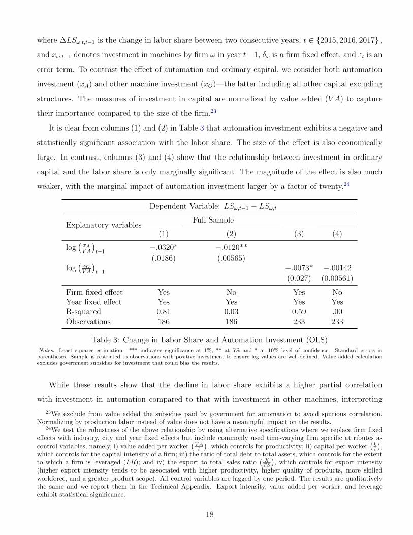
where ∆LSω,t,t−1 is the change in labor share between two consecutive years, t ∈ 2015, 2016, 2017 ,
and xω,t−1 denotes investment in machines by firm ω in year t−1, δω is a firm fixed effect, and εt is an
error term. To contrast the effect of automation and ordinary capital, we consider both automation
investment (xA) and other machine investment (xO)—the latter including all other capital excluding
structures. The measures of investment in capital are normalized by value added (V A) to capture
their importance compared to the size of the firm.23
It is clear from columns (1) and (2) in Table 3 that automation investment exhibits a negative and
statistically significant association with the labor share. The size of the effect is also economically
large. In contrast, columns (3) and (4) show that the relationship between investment in ordinary
capital and the labor share is only marginally significant. The magnitude of the effect is also much
weaker, with the marginal impact of automation investment larger by a factor of twenty.24
Dependent Variable: LSω,t−1 − LSω,t
Explanatory variablesFull Sample
(1) (2) (3) (4)
log(xAV A
)t−1
−.0320* −.0120**
(.0186) (.00565)log(xOV A
)t−1
−.0073* −.00142
(0.027) (0.00561)
Firm fixed effect Yes No Yes NoYear fixed effect Yes Yes Yes YesR-squared 0.81 0.03 0.59 .00Observations 186 186 233 233
Table 3: Change in Labor Share and Automation Investment (OLS)Notes: Least squares estimation. *** indicates significance at 1%, ** at 5% and * at 10% level of confidence. Standard errors inparentheses. Sample is restricted to observations with positive investment to ensure log values are well-defined. Value added calculationexcludes government subsidies for investment that could bias the results.
While these results show that the decline in labor share exhibits a higher partial correlation
with investment in automation compared to that with investment in other machines, interpreting
23We exclude from value added the subsidies paid by government for automation to avoid spurious correlation.Normalizing by production labor instead of value does not have a meaningful impact on the results.
24We test the robustness of the above relationship by using alternative specifications where we replace firm fixedeffects with industry, city and year fixed effects but include commonly used time-varying firm specific attributes ascontrol variables, namely, i) value added per worker
(V Al
), which controls for productivity; ii) capital per worker
(kl
),
which controls for the capital intensity of a firm; iii) the ratio of total debt to total assets, which controls for the extentto which a firm is leveraged (LR); and iv) the export to total sales ratio
(XTS
), which controls for export intensity
(higher export intensity tends to be associated with higher productivity, higher quality of products, more skilledworkforce, and a greater product scope). All control variables are lagged by one period. The results are qualitativelythe same and we report them in the Technical Appendix. Export intensity, value added per worker, and leverageexhibit statistical significance.
18
the automation investment coefficient in terms of structural parameters is fraught with problems.
First, OLS does not address the issue of causality, i.e. changes in labor shares and investment in
automation are endogenous responses of firms to changes in goods and factor prices, and so we need
exogenous variation to provide evidence of a causal effect of automation on the labor share. Second,
even with an instrument to uncover causality, we need a specification informed by a structural model
in order to estimate key parameters of the model. The next section discusses how we address these
challenges using subsidies for automation as an instrument in a 2SLS setup.
2.3 Identifying the effect of automation: theory
The equations derived in lemmas 2 and 3 readily suggest a path to estimate the causal impact
of automation on the labor share and the average elasticity E [σω] by using the observed variation in
subsidy rates sω as an instrument.25 Indeed, from (11) and (14) we know that sω affects the labor
share only through its impact on the m/l ratio. Accordingly, a subsidy rate that is appropriately
orthogonal to the firm’s parameters and shocks can be used as a valid instrument to identify the effect
of automation on the labor share. However, using these lemmas for the estimation is not possible in
practice. First, we do not observe the terms LSO (ω, t) and LSN (ω, t) in the right-hand side of (14).
As a result, we cannot compute the dependent variable in the second-stage regression. Second, we
do not have reliable information on the stock of automation capital. We now show how this theory
can be extended to estimate the effect of automation using the data that we have.
In what follows, let τ denote the three-year period 2015-2017 covered by the survey, and τ − 1
denote the previous three-year period (which, in principle, we do not observe). Unless otherwise
noted, we compute flows in period τ as the discounted sum of the flows for the years 2015, 2016 and
2017 (defined precisely in the next section). For stocks, we take the average of the three years. To
calculate the change in the labor share across periods—lacking data for the preceding period—we
take the difference between endpoints; that is, years 2017 and 2015. Such an approach, if anything,
likely understates the change in the labor share and would work against finding a strong effect of
automation.
25Throughout, we work with an expectation operator E [x] that is to be understood as the mean value of anyvariable or parameter x across all firms:
x := E [x] =1
n
∑i
∑c
∫ω∈Ωci
x (t, ω) dω,
and analogously for any conditional expectation operator.
19

Assumptions
To obtain identification, we impose two assumptions on the relationship between the subsidy rates
and other elements of the model. We will discuss the empirical relevance of these assumptions in the
next section.
Our first assumption is on the probabilistic structure of the subsidies.
Assumption 1. The subsidy s (τ, ω) follows the process
s (τ, ω) = si (τ) + sc (τ) + εs (τ, ω) , (17)
where si and sc are industry- and city-specific mutually independent stochastic processes and εs (τ, ω)
is a mean-zero i.i.d. firm-specific stochastic process.26
Our second and key identifying assumption requires that the subsidy residual εs (τ, ω) be orthog-
onal to other exogenous variables or parameters.
Assumption 2. The random process εs (τ, ω) is orthogonal to any parameter, shock or factor price
(or their combination) z (t, ω) in the sense that
E [z (t, ω) |εs (τ, ω)] = E [z (t, ω)]
for all t.
The above assumptions play a key role in our analysis. They ensure that the residual of the subsidy
rate, after being projected onto city and industry fixed effects, satisfies the exclusion restriction for
instrumental variable (IV) estimation. Note that the second assumption applies not only to the
exogenous variables but also to the endogenous wage rate w, to industry-level price indices, as well as
to the subcomponents of the subsidy: si and sc in equation (17). This requires the subsidy program
to be relatively small compared to the size of the relevant markets, including the labor market, so
that the subsidy residual εs does not move these equilibrium objects “too much.” Since the mean
of the residual is zero, and only a fraction of firms are subsidized, we do not consider this to be a
serious limitation. In the quantitative section we will nonetheless test the validity of this assumption
using our calibrated model.
26Proofs also assume finite moments as appropriate.
20

Furthermore, Assumption 2 implies that previous subsidy rates, which act as parameters, are
similarly orthogonal to the residual εs (τ, ω). While we view this assumption as reasonable, we show
in Appendix D that the estimates presented below are conservative, in the sense that they provide a
lower bound on the mean elasticity of substitution E [σω], so long as the residuals εs (τ − 1, ω) and
εs (τ, ω) are positively correlated.
Identification results
We next work out the link between a firm’s investment in automation capital to the investment
subsidy it faces. The result holds up to a first-order approximation (denoted by the symbol ≈) of
the left-hand side of 14 and of the firm’s policy functions with respect to the subsidy rate s. We also
validate these approximations using numerical simulations of our model in the next section.
To be consistent with the institutional framework described in Section 2.2, we focus on investment
decisions between two periods τ − 1 and τ , defined as
x (τ, ω) := pm (τ)m (τ, ω)− (1− δmi ) pm (τ − 1)m (τ − 1, ω) . (18)
The following lemma relates investment x (τ, ω) to the subsidy residual.
Lemma 4. The automation investment intensity is related to the subsidy residual through the equation
E[x (τ, ω)
l (τ, ω)|εsω (τ, ω)
]≈ Lεsω (τ, ω) + cte, (19)
where L and cte are some constants.
This lemma is analogous to Lemma 2 and the same intuition applies, with the crucial difference
that here it involves the investment rate x normalized by labor employed in production instead of
the stock of automation capital m.
We now turn to our second result that links the conditional expectation of the change in a firm’s
labor share to the conditional expectation of its investment in automation.
Lemma 5. The change in the labor share is related to automation investment intensity through the
equation
E [LS (τ, ω)− LS (τ − 1, ω) |εsω (τ, ω)] ≈ BE[x (τ, ω)
l (τ, ω)|εsω (τ, ω)
]+ cte (20)
21

where cte is a constant and where B is another constant given by
B = − 1
1− s1
L
(1
LS − LSN+
1
LSO − LS
)−1
E [σω − 1] , (21)
where s is the mean subsidy rate across firms, LS is the average labor share, and LSO and LSN are
the averages of (4) and (15), respectively.
The constant terms s, LS, LSN and LSO are the points around which first-order approximations
are taken. We have some flexibility in choosing their values, but to minimize the approximation error
they should be as close as possible to the actual observations, and the mean values are a natural
choice.
The following proposition puts the two lemmas together to form the basis for our IV estimation
in the next section.
Proposition 1. The coefficients B and L can be consistently estimated from a two-stage least squares
regression of the form:
LS (τ, ω)− LS (τ − 1, ω) ≈ cte+ Bx (τ, ω)
l (τ, ω)+ FEi + FEc + e (ω) , (22)
x (τ, ω)
l (τ, ω)≈ cte+ Lsω + FEi + FEc + u (ω) , (23)
where e and u are error terms, B is given by (21) and FEi, FEc are a set of industry and city fixed
effects, respectively.
This proposition shows that we can consistently estimate the causal impact of a change in automa-
tion investment on the labor share using the subsidy sω as an instrument. Furthermore, it implies
that we can back out the average elasticity estimate from the estimated regression coefficients using
the formula
σ := E [σω] = BL (1− s)(
1
LS − LSN+
1
LSO − LS
), (24)
where the coefficients B and L come from estimating the system (22)–(23). The calculation requires
values for s, LS, LSN and LSO. We will describe in the next section how we come up with these
numbers.
22

Measurement error
Before moving to the estimation results, we briefly discuss how robust our identification strategy
is to measurement errors in the subsidy rate and the investment intensity (x/l). This discussion will
be important in the implementation of our approach.
First, measurement errors in the second-stage explanatory variable x/l can be present without
affecting our estimate of E [σω], even if they are of a multiplicative form rather than classical (or-
thogonal additive noise). In other words, measuring c× (x/l) instead of the true investment intensity
x/l is sufficient for identification, as long as c is an orthogonal random variable with a positive mean
that satisfies Assumption 2. The reason for this is that the identification of the average elasticity
E [σω] involves the product BL and, by (19) and (20), the same measurement error appears on the
left- and right-hand side of the two equations for a null effect on the product itself. In particular,
we can readily see that estimating the first stage with the mismeasured investment rate c × (x/l)
will yield the coefficient L′ = L/E [c] while the second stage will yield the coefficient B′ = BE [c],
implying L′B′ = LB. Adding classical measurement error to this relation, that is, c×(x/l)+ d, would
not change this conclusion because the IV removes this kind of measurement error.27
Second, measurement errors in the subsidy rates sω do not invalidate our identification of the
second-stage coefficient but may invalidate the estimate of the elasticity, to the extent that measure-
ment errors bias the first-stage coefficient L without an offsetting effect on the second-stage coefficient
B. For example, suppose that the econometrician observes s′ = b × s, where s is the true subsidy
rate that enters the decision process of the firm and where b is a constant or some i.i.d. random
variable. Then, since the left-hand side of (23) is the outcome variable, the first-stage coefficient L′
will be L′ = E[Lb]. However, the predicted values of x/l will be unchanged and so the second-stage
regression of 2SLS will not change, implying a biased point-estimate of E [σω] by (24). Classical
measurement errors (orthogonal additive noise) are of a lesser concern here. Such an error will result
in an attenuation bias in the first-stage coefficient, but the same attenuation bias will tend to have
an offsetting effect on the second-stage coefficient by reducing the variation of the predicted value of
the explanatory variable in the second stage (x/l).
27If c is a random variable that is correlated with x/l, however, we would only recover the coefficient in the secondstage as long as the error term of the linear projection of c × (x/l) onto x/l has desirable properties, otherwise ourestimation may be biased simply because the linearity assumption is not valid.
23

2.4 Estimation results
In this section, we employ Proposition 1 to estimate the causal effect of automation investment
using two-stage least squares regressions. The dependent variable is the change ∆LS (ω) in the labor
share of a firm ω between 2015 and 2017.
Specification using firm-level subsidies
We begin with the most basic specification that uses the average subsidy rate calculated for each
firm individually as an instrument for automation investment per production worker, x/l. We con-
struct this subsidy rate by averaging the subsidy rates reported by each firm for the years 2015, 2016
and 2017. The subsidy rate for a firm in a given year is calculated by dividing the subsidy payments
self-reported by the firm for purchases of automation capital by its total automation investment in
that year. 28
As for the variable we instrument for, we consider two specifications. The first adheres closely
to the theory and uses total investment in automation over the entire sample period for each firm
individually, deflated by the CPI and depreciation rate, and divides it by the corresponding average
employment in production between the years 2015 and 2017. Formally, let δm be the depreciation rate
of automation capital and let πt be the CPI inflation in each year.29 Let the cumulative investment
in 2015 renminbi (RMB) between years T and T be
xT−T (ω) :=
∑t=T ,...,T x (ω, t)
(1−δm1+πt
)T−t1 + T − T
,
where xt is the surveyed firm’s nominal spending on automation purchases in RMB. The first speci-
fication uses x15−17 (ω) /l15−17 (ω) as instrument, where l15−17 is the average in production labor over
those years.
Our second specification relies on the ratio x17 (ω) /l17 (ω) instead, and effectively treats 2015
and 2016 as predetermined years. The reasoning behind this specification is that since MIC was
announced in mid-2015 and effectively started to come online throughout 2016, investment rates
28Alternatively, one can take the sum of subsidies and investment for all years and then take the ratio. Thisspecification leads to qualitative similar coefficients but to smaller standard errors. See the Technical Appendix forthese results.
29We set δm = 10% following Table C.1-5 “List of depreciation rates under the new asset code classification —Industrial machinery” from the Bureau of Economic Analysis. We use the Consumer Price Index (All Items for China,Index 2015=100, Annual, Not Seasonally Adjusted Values): CPI(2015) = 1, CPI(2016) = 1.02, CPI(2017) = 1.03625.Source: Economic Research Division, Federal Reserve Bank of St. Louis.
24
prior to 2017 might not reflect the impact of the subsidies and, as a result, only adds noise to the
estimation of the first stage at the expense of not exactly adhering to the theory’s implied relation in
the second stage.30 Depending on how important these errors are this may increase statistical power.
As discussed, the IV deals quite well with measurement errors implied by not exactly adhering to
the theory-implied law of motion.
The results of the 2SLS estimation for both specifications are shown in Table 4. We focus on the
intensive margin of automation investment and therefore restrict the sample to firms with positive
investment. In line with the model and Assumption (2), we include city and industry fixed effects,
and so our identification relies on the variation in subsidies that are not captured by these fixed
effects. We also include value added as a regressor to control for firm size.
The results show that the first specification suffers from low statistical power. This may indicate
that the early years in our sample firms were not affected by the subsidies yet. The coefficients
are significant but only at the ten percent level. The F-statistic is quite low and indicates a weak
instrument. In contrast, the specification that drops the years 2015 and 2016 from the investment
variable fares significantly better in terms of coefficient estimates, although the instrument is still
somewhat weak. We will consider an alternative specification with stronger instruments in the next
section to address this shortcoming and other concerns.
The results of Table 4 are robust to various changes in the specifications. In the Technical
Appendix we show that dropping the size of the firm as a control has no meaningful impact on the
results. The point estimates are stable with and without fixed effects and across the two specifications.
Finally, we check for heteroscedasticity in the error terms using the Pagan-Hall test. We find p-values
close to 1 so that we cannot reject the null hypothesis that the error terms are homoscedastic.
In all the specifications included in Table 4, the signs of the coefficients are consistent with an
30Investment decisions are planned ahead of time, and while some firms might have received a subsidy in 2016, itneed not imply that the subsidy drove their investment decision back in 2016. Decisions in 2015 are unlikely to havebeen influenced at all by MIC since the program was announced in 2015. For this reason the first stage under thesecond specification may have more statistical power. The second stage will involve mismeasurement because it nolonger adheres to the laws of motion implied by theory. For this measurement error not to become a problem it mustbe that the linear projection of one variable onto the other,
x17
l17= aω
(x16−17
l15−17
)+ ai + ac + eω,
satisfies Assumption 2 (the error term e and the coefficient of the projection (eω, aω) must both be orthogonal to thesubsidy residual). This follows from the second part of the proof of Proposition 1 (version of Frisch–Waugh–Lovelltheorem), the discussion of measurement error in that section, and the fact that IV estimation removes the attenuationbias normally implied by the presence of classical measurement error e. We omit the formal proof.
25

(1) (2) (3) (4) (5) (6)
Second-stage dependent variable∆LSω = LSω (2017)− LSω (2015)
Automationinvestment(x15−17/l15−17)
−0.0659* −0.0725* −0.070**
(0.034) (0.041) (0.045)
Automationinvestment(x17/l17)
−0.053** −0.054** −0.043**
(0.023) (0.029) (0.020)
First-stage dependent variableAutomation investment (x/l)
Subsidy rate(s)
4.867* 4.455* 3.853* 6.022*** 6.372** 6.086***
(2.6) (2.36) (2.36) (2.15) (2.65) (2.76)
Industry / cityfixed effects
No/Yes Yes/No Yes/Yes No/Yes Yes/No Yes/Yes
Size (log VA) Yes Yes Yes Yes Yes Yes# observations 143 143 143 143 143 143F -statistic 3.5 3.5 2.9 7.9 5.8 4.9
σ (LSO = 0.6) 4.27 4.30 3.75 4.25 4.51 3.67σ (LSO = .66) 3.43 3.44 3.04 3.41 3.61 2.98
Table 4: Impact of Automation on Labor Share using Firm-level Subsidies As InstrumentNotes: Two-stage least squares estimation (2SLS). *** indicates significance at 1%, ** at 5% and * at 10% level of confidence. Robuststandard errors in parentheses. Sample is restricted to observations with positive automation investment. The instrument is the subsidyrate on firm-level calculated by taking the ratio of subsidy received for purchases of automation capital (as defined in text) and totalinvestment during the sample period.
elasticity of substitution between labor and automation capital that is larger than 1. Our
estimation therefore suggests that higher automation investment has a negative and sizable effect
on the labor share. We can see this through a back-of-the-envelope calculation. Using the most
conservative coefficients in Table 4, the estimates imply that a 1 percent subsidy, or decline in the
price of automation equipment, leads to a decline in the labor share of
0.043× 6.086× 1% = 0.26%—a large number. We can put this number in perspective through the
following back-of-the-envelope calculation. Suppose that the price of automation capital declines by
80 percent, which is well within the range of industry quality-adjusted estimates since the 1990s
(see discussion in footnote (6)). Then, our results would imply a decline in the labor share across
automating firms in manufacturing by 20.8 percentage points. To give an order of magnitude, the
26

aggregate labor share declined by about 12 percentage points from 1990 in the United States.
That being said, the above back-of-the-envelope calculation needs to be taken with a grain of salt.
First, the coefficients of Table 4 pertain to a locally identified partial equilibrium effect that does
not take into account offsetting forces, in particular the adjustment of prices and wages, that may
be dampening the overall effect. Second, our estimation only covers manufacturing firms that
(actively) invest in automation. Since these firms have witnessed a larger decline in their labor
share, our estimates would predict a much smaller decline when considering all manufacturing
firms. Third, we used linear approximations to derive our structural equations and these
approximations might lose their validity for large changes occurring over decades. We will come
back to the aggregate impact of automation prices when we explore the calibrated version of the
model in the next section.
Structural interpretation of the estimated coefficients
We now combine the estimates from Table 4 with equation (21) to obtain a structural estimate
of the average elasticity of substitution between labor and automation capital, given by the equation
σ := E [σω] = −BL (1− s)(
1
LS − LSN+
1
LSO − LS
)+ 1, (25)
where, recall, B is the second-stage coefficient on automation investment, and L is the first-stage
coefficient on the subsidy rate. Since our identification comes from automating firms, we approximate
the expressions around s = 0.12, which is is the average subsidy across firms receiving a subsidy, and
LS = 0.485, which is the average labor share across automating firms in 2017. As for the labor share
of nonproduction workers, we use .33, which is the value reported in Table 2 for automating firms.
Computing the average elasticity σ from (25) requires a value for LSO, which, recall, would be
the average labor share if the firms were not using any automation capital in production (m = 0).
Given our estimated coefficients, the expression (25) is decreasing in LSO, such that higher values
of LSO are pushing for lower elasticities of substitution. Since LSO is a counterfactual quantity, we
have no hope of directly observing it in the data. In the next section, we use the calibrated model
to find a consistent value with the data, and find that LSO= 60% provides the best fit. Here, we
also report estimates of E [σω] using the textbook value of the labor share of LSO = 66%. We view
this number as quite conservative for two reasons. First, in the presence of profits, the value of LSO
is bounded from above not by one but by a lower number that accommodates markups. Second,
27

the manufacturing labor share in China was 57% in 1997—when very few, if any, modern industrial
robots were at work.31 On the other hand, the US labor share back in the 1960s was close to the
textbook value. To the extent that US history is a better indicator, the value of LSO = 66% is
nonetheless appropriate.32
We report the estimates of E [σ] in the last rows of Table 4. For the textbook value of the
labor share, LSO = 66%, the average elasticity ranges from 3.0 to 3.6. For our baseline value of
LSO = 60% the analogous range is from 3.7 to 4.5. Importantly, all values are above 1, confirming
that a decline in the price of automation equipment has a negative effect on the labor share. They
are also relatively large, but in drawing such a conclusion one should keep in mind the magnitude
of the decline in the US manufacturing labor share.33 We return to the discussion of the estimated
elasticity of substitution in the quantitative section.
Regression setup using city-industry average subsidies
Investment decisions are affected by the subsidy rate that the firm expects to receive for these
investments and not the subsidy that the firm actually received. We do not observe these expectations
and proxy for them using information available in the data. In the previous section we relied on the
observed subsidy payments received by the firms to compute the subsidy rate and assumed that what
firms expected to receive is equal to what the firms actually received. But if firms which received
zero subsidies ex post did not expect such an outcome ex ante, or firms which received full subsidy
considered the risk of receiving zero subsidy ex ante, the measurement of subsidy rate could induce
a bias that is multiplicative, and as explained in the previous section, such a bias could adversely
affect the estimated elasticity.34 For this reason, we consider an alternative instrument computed
by averaging the subsidy rates reported by all the firms in a given industry-city grouping, and then
applying it to all firms for that grouping. This addresses the problem since the average realization
31Data from the China Statistical Yearbook, 1997.32 Kehrig and Vincent (2018) report that the labor share in U.S. manufacturing declined from 61 percent in 1967
to 41 percent in 2012, which would suggest that historic evidence from the U.S. points to a higher value. By thismeasure, then, the textbook number of LSO = 66% would be a conservative upper bound.
33Since the 1990s the US labor share index in manufacturing declined by 19% according to U.S. Bureau of LaborStatistics “Productivity and Costs” (1990-2018). See also discussion in footnote 32.
34It is possible that firms are simply misreporting the subsidy payments that they receive for their investments. It isalso possible that, when making investment decisions, firms were facing some uncertainty about the size of the subsidypayments that they would receive. In either case, averaging the firm-level rates across all firms in a city-industrypair might get us closer to the true policy subsidy that was expected by the firms. Finally, it is possible that somefirms might have “lobbied” for more generous subsidies for themselves, perhaps introducing an undesirable correlationbetween subsidies and other firm characteristics. This second instrument would also alleviate these concerns.
28
of any random variable should bring us closer to its ex ante expectation. In other words, if the
coefficients do not change, this is an indication that our estimates are immune to this problem.
An additional advantage of this setup is that it increases the statistical power since more firms are
“effectively” subsidized.
Formally, for any given city-industry pair (c, i) and year t ∈ 2015, 2016, 2017, we construct the
instrument for a firm ω as follows:
sΩciω =
∑2017t=2015
∑ω∈Ω′ci
Sci (t, ω)∑2017t=2015
∑ω∈Ω′ci
xci (t, ω),
where Sci (t, ω) is the subsidy transfer (in RMB) deflated by the CPI inflation and reported by firm
ω from city c and industry i in period t, xci (t, ω) is automation investment similarly deflated by CPI;
the set Ω′ci ⊆ Ωci includes all automating firms from city-industry pair (c, i). To back out the average
elasticity in this case, we use s = 0.109 and otherwise the analysis is unchanged.
The regression results are presented in Table 5. The estimated coefficients are similar across
different variants in terms of their product and also similar to those reported in Table 4. The
standard errors are however smaller with several coefficients significantly different than zero at the
1 percent threshold. Statistical power also increases, and the F-statistics are indicative of a strong
instrument for two specifications, including for our preferred specification that uses city and industry
fixed effects in column 6. The estimated elasticities E [σω] are similar to those of Table 4. 35
Differential impact of ordinary capital
For completeness, we ran an analogous exercise for ordinary capital (Machine-3), for which we
also have capital-type specific subsidy information. We found coefficients to be insignificant.36 To-
gether with our previous OLS results, this indicates an important difference between ordinary and
automation capital: while we find that automation capital has a clear negative impact on the labor
share, there is no evidence that ordinary capital has a similar effect.37
35Controlling for size of the firms using value added does not have a meaningful impact on the results.36See the Technical Appendix.37The lack of significance in this case may indicate that the instrument is not relevant and it should not necessarily
be interpreted as evidence against any relationship between price of capital and the labor share.
29

(1) (2) (3) (4) (5) (6)
Second stage dependent variable∆LSω = LSω (2017)− LSω (2015)
Automationinvestment(x15−17/l15−17)
−0.0928* −0.0815* −0.0734*
(0.051) (0.045) (0.045)
Automationinvestment(x17/l17)
−.0382*** −.0458* −.0377***
(0.014) (0.026) (0.012)First stage dependent variableAutomation investment (x/l)
Subsidy rate(sΩciω )
3.584 4.319** 3.838* 7.772*** 6.401** 7.092***
(2.26) (2.13) (2.36) (2.15) (2.65) (2.76)
Industry / cityfixed effects
No/Yes Yes/No Yes/Yes No/Yes Yes/No Yes/Yes
Size (log VA) Yes Yes Yes Yes Yes Yes# observations 143 143 143 143 143 143F -statistic 3.5 3.5 2.9 20.8 5.6 14.9
σ (LSO = 0.6) 4.44 4.64 3.91 4.06 4.03 3.76σ (LSO = .66) 3.55 3.70 3.16 3.28 3.25 3.05
Table 5: Impact of Automation on Labor Share using City-industry Average Subsidies as InstrumentNotes: Two-stage least squares estimation (2SLS). *** indicates significance at 1%, ** at 5% and * at 10% level of confidence. Robuststandard errors in parentheses. Sample is restricted to observations with positive automation investment. The instrument is the subsidyrate on firm-level calculated by taking the ratio of subsidy received for purchases of automation capital (as defined in text) and totalinvestment during the sample period.
2.5 Limitations and robustness
We conclude this section by discussing further limitations of our instrument and discuss how we
addressed them.
First, it is possible that subsidies during the sample period may be correlated with some other
subsidies that were previously in place. Our theory, recall, assumes that preexisting subsidies are
uncorrelated with the residual of the current set of subsidies after controlling for city and industry
fixed effects. While we are unaware of any previous major national initiative that specifically targeted
automation investment on that scale, other economic policies were in place in China before MIC 2025
and it is possible that some small subsidies for automation were also in place. We investigate how
this would affect our results in Appendix D and find that, in the likely case of a positive correlation
30

between the residuals of the pre-existing subsidies and subsidies under MIC 2025, our estimation of
the average elasticity σ would be biased downward, providing a lower bound for the true elasticity.
Since we find high values to begin with, this does not change the conclusions from our findings.
Intuitively, a positive correlation reduces the link between current subsidies and labor share changes
as the firm would have already responded to the subsidies.
Second, subsidy programs may have targeted specific firms or industries whose labor shares have
been changing for reasons unrelated to their investment in automation. In this case, our instrument
would mistakenly identify a causal link between automation and the labor share where none exists.
We have read through official documentation and found no evidence of this type of policy being used
to target specific firms, albeit there exists a possibility that this is the case because subsidized firms
tend to be larger. But as is clear from the regression, controlling for size does not make a difference.
We also show in the Technical Appendix that including controls for party connections and “lobbying
power” do not invalidate our results.
3 Quantitative results
In this section we calibrate our model using a simulated method of moments and conduct two
exercises using the calibrated economy. First, we analyze the consistency of our estimate micro
elasticity of substitution σ with the macroeconomic changes observed in the sample. These aggregate
changes involve not only the firm-level elasticity but also patterns of substitution across firms so that
the full model is needed to capture the aggregate impact of a change in automation prices. Second, we
validate our identification procedure on model-generated data. We find that despite the assumptions
that our identification involves, our reduced-form empirical strategy is quite robust and can accurately
back out the true elasticity of substitution even in the presence of large parameter heterogeneity. In
what follows, unless explicitly noted, all mean values calculated across firms are weighted using the
value added.
3.1 Parameterization
The setup of the model is as described in Section 1. While our exercise focuses on automating
firms, we include firms that cannot automate (aω = 1) to study the model’s implications for the
whole sample. The presence of these firms only matters for the general equilibrium feedback between
31

automation and prices.
Sample structure
The model’s time horizon is infinite but, as before, we focus on two subsequent periods: a pre-
subsidy period “τ − 1” and a post-subsidy period “τ .” We rely on the differences between values in
the years 2015 and 2017 and relate those to model-implied differences between τ and τ−1. The model
is designed to approximate the city-industry structure of our dataset. As in the data, there are 44
cities, 23 industries, and 117 city-industry groupings. To avoid random variation induced by the small
numbers of firms in the sample, and also balance the computational load of solving for equilibrium
repeatedly, we double the number of firms in the model and include 351 automating firms—three per
grouping—and 3,192 firms in total—14 per grouping. Including additional firms is useful to remove
variation coming from a particular draw of random numbers, and increasing the sample size further
has a small impact on the statistical properties of the model. We calculate model-generate moments
using the full sample as opposed to bootstrapping the values. However, when we run regressions on
model-generated data to test our empirical strategy we draw a sub-sample of size consistent with the
data and bootstrap the estimates.
Setting the share of automation activities a < 1 is insufficient to ensure that a firm automates
(invests in automation capital) in the model. For instance such a firm facing a negative demand
shock might not want to invest to increase its size. To ensure a consistent number of automating
and nonautomating firms, we therefore pick firms at random from a larger pool to ensure that we
populate each grouping as specified (three automating firms per grouping). This selection procedure
is a function of equilibrium prices and it is part of the fixed point to solve the model. By construction,
then, automating firms are the ones which do not experience large negative shocks in period τ .
Technology parameters
We fix markups at 33% for each firm, implying a constant θ that solves θθ−1
= 1.33. This level of
markups is consistent with the aggregate operating (pre-tax) income of automating firms relative to
their value added that we see in our data.38
To model firm-level heterogeneity in α, γ, η, we assume that these technology parameters follow
38We calculate the Lerner index as the ratio of operating income to value added. Operating income corresponds toitem D.3 in the enterprise cost and profit statement questions in the questionnaire. The questionnaire can be foundin the supporting files.
32
independent beta distributions with shape parameters ζ1 (h) and ζ2 (h) for h ∈ α, γ, η.39 To restrict
the amount of parameters to calibrate, we further assume that α and γ follow the same distribution.40
Our calibration strategy takes advantage of the fact that, in the model, the mean of various
quantities is related to the average pre-automation labor share LSO. We write these means in terms
of LSO and then pick that last quantity to best fit the data, which corresponds to the value LSO = .6
used in the previous section. For instance, we know from (4) that
α = γ = 1− θ
θ − 1LSO = 1− 1.33LSO,
where the overline · denotes the value added-weighted average. For a given value of LSO, we can
use that equation to discipline the shape parameters of the distributions of α and γ.
We proceed similarly to discipline the distribution of η. To calculate the mean value η, we note
that automation in the model reduces the labor share from its automation-free level LSO by lowering
the labor share of production workers according to the relation LSτ −LSO = LSP τ −LSOP , where,
as defined in (4), LSOP := θ−1θ
(1− η) (1− α) . Given the calculated value added-weighted data
averages for LSτ = .485 and LSP τ = .345 across automating firms in 2017 (see Table 2), and
together with (4), we obtain
η = 1− LSOP
LSO= 1− .345 + LSO − .485
LSO=
.155
LSO.
Finally, we set the value of the elasticity of substitution σ as a function of LSO using the es-
timated coefficients from our city-industry regression that includes all fixed effects (our preferred
specification). We assume that this elasticity is identical across firms, sectors and cities. Equation
(24) states the relationship between σ and LSO.
Our estimation procedure varies, among other things, LSO to match a set of moments. While the
parameters are jointly estimated, LSO has a particular importance for one key targeted moment: the
39We normalized the distributions to the interval [0.05, 0.95] to avoid issues with parameter values that are too closeto the extremes. To do so, we use the transformed random variable Y = X(b− l) + l, where b = .95 and l = .05, andX is a beta distributioned on [0, 1].
40This assumption is motivated by the data. In the presence of heterogeneity in η, any large differences in themean values of α and γ would imply a nonzero correlation between the labor share and the importance of productionactivities in firms’ overall operations. For example, if we assumed α = 1/3 and set γ close to zero, we would see thatfirms which do not have many production activities have a much lower labor share, as in their case α would be ofgreater importance for the division of income between labor and capital. Similarly, a strong correlation between α andγ would induce a high labor share among firms with a large share of production activities. Since we are not aware ofsuch patterns in historic data, we choose independent distributions with equal shape parameters.
33

average growth rate of value added produced by automating firms. Below, we describe the mechanism
through which LSO affects that quantity and why that parameter is properly identified through the
estimation procedure.
The choice of LSO pins down the mean values of α, γ and η but more data is needed to pin down
the variance of these parameters and hence their distribution. To do so, we choose two data targets
that are particularly relevant: 1) the coefficient of variation of the share of production activities
as measured by the ratio of production employment to total employment (SPE17) of .25 in 2017
(which we associate with period τ); 2) the coefficient of variation of the ratio of the labor share of
production employees to the labor share of nonproduction employees of 1.0 in 2017. Together with
the mean values listed above, these targets identify ζ1 (h) and ζ2 (h) for h ∈ α, γ, η (recall that the
distributions of γ and α are assumed identical).
Shocks and trend growth rates
We target moments related to the growth of value added and the initial employment distribution
across firms to pin down d and A. Since d and A are equivalent in the model, we use d to model the
dispersion of employment across firms and shocks across periods. We use A to model the relative size
of automating firms relative to non-automating firms and the growth rate of wages (and productivity)
in the economy as a whole.41
Specifically, the initial value of log (d (ω, τ − 1)) ∼ iid N(0, σd(τ−1)
)is log-normally distributed
with a standard deviation σd(τ−1) that is set to match the coefficient of variation of total employment
across automating firms in 2015, which we find to be close to 1. Since automating firms account
for 23.5 percent of value added produced by all firms in 2017, we normalize A (ω, τ − 1) = 1 for
nonautomating firms and set the TFP of automation firms to a constant A (ω, τ − 1) = A > 1 that
is large enough to hit this target.
To capture shocks that affect idiosyncratic differences in firm growth rates, we assume that the
demand shifter log (d (ω, τ)) ∼ iid N(log (d (ω, τ − 1)) , σd(τ)
)is log-normally distributed around the
previous value d (ω, τ − 1), implying a random walk process for the evolution of firm sizes. We choose
the standard deviation σd(τ) that matches the standard deviation of the firm-level growth in value
added between 2015 and 2017, which in our data is .55. The period τ productivity A is assumed to
41The distinction between A and d would have mattered had d been assumed to be “quality” reflected in the priceof the good, which we did not assume by treating it as a “hidden” preference parameter. “Quality” shocks in ourmodel are captured by a markup shock.
34

grow at a constant rate across all firms so that the model exactly matches the average growth rate
of manufacturing real wages in China of 12.5 percent between 2015 and 2017.42
User cost of capital
We use (5) to compute the user cost of each type of capital. We assume that the real cost of
funds is 6 percent on an annual basis, which is based on the estimated emerging weighted average
cost of capital (WACC) for 2016.43 We assume that the annual depreciation rates are 5 percent
for structures–which we associate with support capital ks—and 10 percent for equipment ke and
automation capital m.44 These numbers are not particularly important for the results. We assume
that they do not change over time and are common across firms and sectors. We compound annual
rates to arrive at three-year equivalents for the model.
To get the user cost of automation capital from (5) also requires information about the price of
capital pm (τ) to other machinery and the subsidy rate s (τ, ω). Since pm (τ) in the model and the
mean value of the technology parameter a have an analogous effect, we set a = .5 and assume no
dispersion in this parameter for simplicity. We then set the initial price pm(τ − 1) to account for the
2015 value of the labor share of automating firms in the data, and which is 0.5. This target implicitly
determines how much automation capital (mτ−1) automating firms had as of 2015 to bring down the
value of their labor share LS (ω, τ − 1) from the automation-free reference value LSO (ω).
Finally, the subsidy rate s (τ, ω) is assumed to vary at the city-industry level with a positive
subsidy received by only those city-industry groupings that receive positive subsidies in the data.
The subsidy rate is drawn from the beta distribution with a mean across subsidized firms within
subsidized groupings of 10.9% and the coefficient of variation of 44%.45
Computing the user cost of capital using equation (5) requires information on pm (τ). Here, we
target the ratio Ewm(ω, τ)/Ewm(ω, τ − 1), where Ew denotes the value added-weighted average, and
require it to be consistent with the average industrial robot density in the Chinese manufacturing
42Wage growth in manufacturing is between 2015 and 2017 for consistency with other variables that are measuredthis way and it comes from the National Bureau of Statistics of China. It is deflated by the all items CPI.
43We use the industry average emerging market dollar estimate of WACC by Aswath Damodaran (NewYork University Stern) for year 2016 after subtracting US inflation of 2 percent (8.05 - 2 = 6.02). Source:http://people.stern.nyu.edu/∼adamodar/... (average without financials).
44The useful life of industrial robots and digitally controlled machinery is about 10 years. See, for example,https://www150.statcan.gc.ca/.... The International Federation of Robotics uses a slightly higher value of 12 years.As for other categories, we take the values from https://assets.ey.com/... (page 37), which reports the useful life forplant, property and equipment in China of 10 years (ke) and 20 years for buildings (ks) (for tax purposes).
45We limit the domain of subsidy rates so that it does not exceed 50 percent and so the beta distribution is definedon the interval from 0 to .5.
35
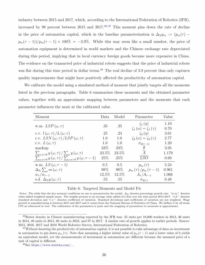
industry between 2015 and 2017, which, according to the International Federation of Robotics (IFR),
increased by 98 percent between 2015 and 2017.46,47 This moment pins down the rate of decline
in the price of automation capital, which in the baseline parameterization is ∆%pm := (pm(τ) −
pm(τ − 1))/pm(τ − 1) × 100% = −3.9%. While this may seem like a small number, the price of
automation equipment is determined in world markets and the Chinese exchange rate depreciated
during this period, implying that in local currency foreign goods became more expensive in China.
The evidence on the transacted price of industrial robots suggests that the price of industrial robots
was flat during this time period in dollar terms.48 The real decline of 3.9 percent thus only captures
quality improvements that might have positively affected the productivity of automation capital.
We calibrate the model using a simulated method of moment that jointly targets all the moments
listed in the previous paragraphs. Table 6 summarizes these moments and the obtained parameter
values, together with an approximate mapping between parameters and the moments that each
parameter influences the most at the calibrated value.
Moment Data Model Parameter Value
w.m. LSP (ω, τ) .35 .35ζ1 (η) 1.10
ζ1 (α) = ζ1 (γ) 0.70c.v. l (ω, τ) /L (ω, τ) .25 .24 ζ2 (η) 3.61c.v. LSN (ω, τ) /LSP (ω, τ) 1.0 1.0 ζ2 (α) = ζ2 (γ) 2.77c.v. L (ω, τ) 1.0 1.0 σd(τ−1) 1.20
markup 33% 33% θ 3.95∑ω:x>0 y (ω, τ) /
∑ω y (ω, τ) 23.5% 23.5% A 1.179∑
ω:x>0 y (ω, τ) /∑
ω:x>0 y (ω, τ − 1) 25% 25% LSO 0.60
w.m. LS (ω, τ − 1) 0.5 0.5 pm (τ) 5.24∆%
∑ωm (ω, τ) 98% 98% pm (τ) /pm (τ − 1) 0.961
wτ/wτ−1 12.5% 12.5% Aτ/Aτ−1 1.066s.d. ∆%y (ω, τ) .55 .55 σd(τ) 0.48
Table 6: Targeted Moments and Model FitNotes: The table lists the key moment conditions we use to parameterize the model. ∆% denotes percentage growth rate. “w.m.” denotesvalue-added weighted sample mean. The weights pertain to an average value added of a firm over the time period 2015-2017. “s.d.” denotesstandard deviation and “c.v.” denotes coefficient of variation. Standard deviations and coefficients of variation are not weighted. Wagegrowth in manufacturing is between 2015 and 2017 and it comes from the National Bureau of Statistics of China. We deflate it by all itemsCPI as referenced in text. The calibration of the parameters is joint and the mapping of parameters to moments is approximate.
46Robot density in Chinese manufacturing reported by the IFR was: 25 units per 10,000 workers in 2013, 36 unitsin 2014, 49 units in 2015, 68 units in 2016, and 97 in 2017. A similar rate of growth applies to earlier periods. Source:2015, 2016, 2017 and 2018 World Robotics Survey, International Federation of Robotics.
47Without knowing the productivity of automation capital, it is not possible to take advantage of data on investmentin automation to pin down pm (τ). Note that assuming a higher initial value of pm(τ − 1) and a lower value of a yieldsan equivalent model, yet the measurements of investment in automation are different because the assumed price of aunit of capital is different.
48See https://www.statista.com/....
36
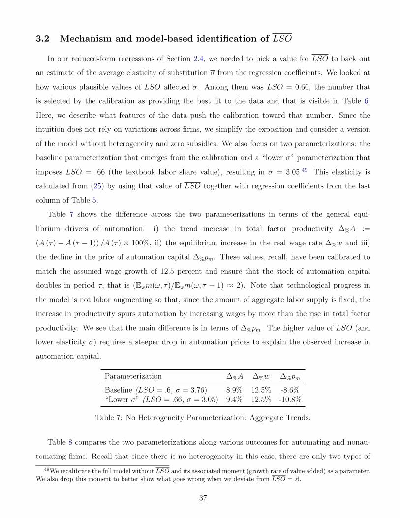
3.2 Mechanism and model-based identification of LSO
In our reduced-form regressions of Section 2.4, we needed to pick a value for LSO to back out
an estimate of the average elasticity of substitution σ from the regression coefficients. We looked at
how various plausible values of LSO affected σ. Among them was LSO = 0.60, the number that
is selected by the calibration as providing the best fit to the data and that is visible in Table 6.
Here, we describe what features of the data push the calibration toward that number. Since the
intuition does not rely on variations across firms, we simplify the exposition and consider a version
of the model without heterogeneity and zero subsidies. We also focus on two parameterizations: the
baseline parameterization that emerges from the calibration and a “lower σ” parameterization that
imposes LSO = .66 (the textbook labor share value), resulting in σ = 3.05.49 This elasticity is
calculated from (25) by using that value of LSO together with regression coefficients from the last
column of Table 5.
Table 7 shows the difference across the two parameterizations in terms of the general equi-
librium drivers of automation: i) the trend increase in total factor productivity ∆%A :=
(A (τ)− A (τ − 1)) /A (τ) × 100%, ii) the equilibrium increase in the real wage rate ∆%w and iii)
the decline in the price of automation capital ∆%pm. These values, recall, have been calibrated to
match the assumed wage growth of 12.5 percent and ensure that the stock of automation capital
doubles in period τ, that is (Ewm(ω, τ)/Ewm(ω, τ − 1) ≈ 2). Note that technological progress in
the model is not labor augmenting so that, since the amount of aggregate labor supply is fixed, the
increase in productivity spurs automation by increasing wages by more than the rise in total factor
productivity. We see that the main difference is in terms of ∆%pm. The higher value of LSO (and
lower elasticity σ) requires a steeper drop in automation prices to explain the observed increase in
automation capital.
Parameterization ∆%A ∆%w ∆%pm
Baseline (LSO = .6, σ = 3.76) 8.9% 12.5% -8.6%“Lower σ” (LSO = .66, σ = 3.05) 9.4% 12.5% -10.8%
Table 7: No Heterogeneity Parameterization: Aggregate Trends.
Table 8 compares the two parameterizations along various outcomes for automating and nonau-
tomating firms. Recall that since there is no heterogeneity in this case, there are only two types of
49We recalibrate the full model without LSO and its associated moment (growth rate of value added) as a parameter.We also drop this moment to better show what goes wrong when we deviate from LSO = .6.
37

Parameterization LSτ−1 ∆LSτ ∆%Lτ yτ−1 ∆%yτ mτ−1 ∆%mτ
A. Baseline (LSO = .6, σ = 3.76)Automating firm .50 -.04 1% 1.33 25% .19 98%Nonautomating firm .60 0. 0% .62 13% 0. -
B. “Lower σ” (LSO = .66, σ = 3.05)Automating firm .50 -.05 5% 1.28 32% .28 97%Nonautomating firm .61 0. 0% .63 .28 0. -
Table 8: No Heterogeneity Parameterization: Firm Dynamics
firms, automating firms and nonautomating firms, and all city-industry groupings are identical.
The table reveals two key differences between the parameterizations, which inform us about the
mechanisms that are behind the identification of LSO—as indicated in Table 6. First, the overall
impact on the labor share of the automating firms, ∆LSτ , is smaller in the baseline parameterization
despite the micro-elasticity σ being higher in that case. To understand this somewhat counterintuitive
outcome, note that the “lower σ” parameterization assumes LSO = .66, so as to get a lower σ from
the same regression coefficient estimates. This implies that, for the model to be consistent with an
initial level of the labor share of LSτ−1 = .5, the initial stock of automation capital (mτ−1 = .28) must
be larger in the “lower” σ parameterization to reduce the labor share from a higher automation-free
value of LSO = .66 and despite a lower sensitivity of the labor share to automation capital due to
the lower σ. Now, since our calibration targets that the stock of automation capital doubles between
2015 and 2017, the larger initial value of mτ−1 implies a larger increase in the stock of automation
capital in absolute terms in the “lower σ” case. As a result, the labor share declines more but also
the value added of firms rises much more.50
As a result, the “lower σ” parameterization implies that the model grossly overshoots the targeted
value of 25 percent increase in total value added produced by automating firms ∆%yτ—which in the
baseline case is targeted to obtain the value of LSO = .6 and in the “lower σ” parameterization
is dropped from calibration targets to accommodate the higher assumed value of LSO = .66 (and
lower σ). To summarize, the lower micro-elasticity σ leads to the inference that firms must have
been much more automated back in 2015, which in combination with the fact that the stock of
automation capital doubled between 2015 and 2017 implies a bigger increase in the value added
produced by automating firms and a larger decline of labor share in these firms.
It is important to note that the data strongly rejects values that would be anywhere near the
50Note that the difference in elasticity is only reflected here in the assumed change in the price of automationcapital. In the “lower σ” parameterization, it is calibrated to decline by ∆%pm = −10.8% while in the baseline caseby ∆%pm = −8.6%.
38

unit elasticity that leads to labor shares that are invariant to the price of automation capital. Such
parameter values would imply an enormous growth of value added produced by automating firms.
Note also that LSO cannot be higher than .7 when average markups are at 33 percent and so the
.66 value that we use in the previous section is close to the upper bound of what is possible given
the assumed level of markups.
3.3 Results
We are now ready to discuss our model’s aggregate implications and to analyze the robustness of
our procedure to estimate the average elasticity σ using model-generated data.
Equilibrium effect of automation
Our reduced-form exercises focused on identifying the microeconomic elasticity of substitution σ.
That number predicts how changes in economic conditions affect the labor share at the firm-level, but
movements in the aggregate labor share depend also on substitution patterns between firms. Here,
we take advantage of our calibrated model to study these patterns and to figure out if our estimated
micro elasticity is consistent with the aggregated changes that we observe in the sample.
Table 10 compares the aggregate predictions of the baseline calibration for firm type. As we can
see, the model does a reasonable job at matching the labor share of automating and subsidized firms
in period τ − 1, while it somewhat missed the labor share of nonautomating firms. Overall, we see
that the model is able to roughly replicate the change in the aggregate labor share between τ and
τ − 1—a key quantity of interest—although its performance for automating and subsidized firms is
better when looking at the unweighted average. When we take all firms together, the unweighted
mean performs slightly worse. What this implies is that larger firms in the data are the ones in
which the labor share is changing more sluggishly than in the model. The last row of Table 9 reports
aggregate automation investment in the model and in the data. As we can see, the model performs
well in this dimension, as it roughly matches the difference between automating and subsidized firms.
One key lesson from Table 10 is that even with a relatively large micro-elasticity of substitution
(σ = 3.76) and large movements in automation prices and productivity, the overall impact on the
labor share is muted. While the labor share of automating firms does decline sizably (by .041), these
firms account for only 23.5 percent of value added so that their impact on the aggregate labor share’s
decline is close to .235 × .041 = 0.0096. We interpret these results as showing that the seemingly
39

large micro-elasticity of σ is roughly consistent with the aggregate patterns in our sample and does
not indicate excessive sensitivity vis-a-vis the data.
StatisticFirm type
Automating Subsidized All
Data Model Data Model Data Model
Agg. labor share in τ − 1 LS (ω, τ − 1) w.m. .500 .500 .502 .505 .496 .573Agg. labor share in τ LS (ω, τ) w.m. .484 .460 .483 .435 .473 .563Change in labor share ∆LSω w.m. -.022 -.041 -.035 -.070 -.026 -.010
∆LSω m. -.036 -.039 -.083 -.065 -.024 -0.004Agg. auto. investment1
∑ω pmxω/
∑ω yω 15.2% 15.2% 22.6% 24.6% 3.6% 3.6%
Table 9: Quantitative Results from the Calibrated ModelNotes: The table compares the baseline calibrated model to the data. ∆% denotes percentage growth rate. “w.m.” denotes value-addedweighted sample mean. The weights pertain to an average value added of a firm over the time period 2015-2017. “m.” denotes (unweighted)mean. Standard deviations or coefficients of variation are not weighted. 1As explained, there is an indeterminacy between the price ofautomation capital and productivity A. We pick the units of automation capital so that the model matches perfectly the aggregateinvestment by automating firms.
Validation of elasticity estimation procedure
Here we use the calibrated model to evaluate the performance of the empirical strategy that
we used in Section 2. That strategy was grounded in Proposition 1, which formally established its
validity under two assumptions. First, it relies on linear approximations of the firms’ policy functions.
Second, it assumes that the subsidy residual εs (τ, ω) from (17) is uncorrelated with various quantities,
among them prices such as the wage rate and the price indices of goods at the city and industry level.
In the calibrated model, these assumptions may only hold approximately. For instance, the linear
approximations are only valid locally and large subsidies might make higher-order terms relevant. In
addition, some prices might be affected by the subsidies, even after controlling for city and industry
fixed effects. To test whether these deviations threaten our estimation procedure, we test their
importance one by one. To simplify the exposition of the main forces at work, we first consider a
version of the calibrated model without parameter heterogeneity. We reintroduce that heterogeneity
later on.
We begin by examining the importance of the linear approximation by considering whether the
first- and second-stage regressions involve data that are related in a linear relationship. That in-
formation is provided by the first two panels of Figure 1. As we can see from the first panel, the
first-stage relationship is roughly linear although there is a slight nonlinearity that might introduce
a bias in the estimation results when the variability of the subsidies across firms is substantial. The
40

second panel illustrates the second stage of our instrumental variable estimation. Here, the model
suggests that the approximation is more accurate, despite the nonlinearity in the first stage, with the
predicted values from the first-stage regression varying roughly linearly with the dependent variable.
The second panel also displays the slope estimated by our IV approaches as well as the slope that
would be estimated using a standard ordinary least squares estimator. In this case, without firm
heterogeneity, the OLS and the 2SLS estimates are very close to each other, which is not surprising.
The third panel of Figure 1 focuses directly on the Taylor approximation that underlies the proof
of Proposition 1 (and Lemma 5); that is, the replacement of
logLSO (τ, ω)− LS (τ, ω)
LS (τ, ω)− LSN (τ, ω)− LSO (τ − 1, ω)− LS (τ − 1, ω)
LS (τ − 1, ω)− LSN (τ − 1, ω)(26)
by a linear approximation that uses LSτ − LSτ−1 and a scaling factor involving mean values of the
involved variables (see (36) in the Appendix). Again, we see that the relationship between these two
quantities is close to linear, and most importantly the slope is approximately one (compared to the
45 degree line indicated in the figure).
To confirm that the slight departure from linearity observed in the first-stage regression does not
introduce a bias in the estimation of σ, we replicate our estimation procedure on model-generated
data and compare the estimated σ to its true value. The results are presented in Table 10. As we
can see, the bias is not very large with an estimated elasticity of σ = 3.8 versus a true value of 3.76.51
We next examine the potential impact of the endogenous response of prices to changes in subsidies.
The fourth row of Table 10 reports the elasticity as estimated on model-generated data when we
counterfactually take the period-τ prices from an economy with zero subsidies, which is labelled
“estimated σ w/ no GE feedback”. As we can see, the estimated elasticity is little changed by using
counterfactual prices and so the general equilibrium feedback effect through prices is quite small.
We repeat the same exercise on data generated from the baseline model with parameter hetero-
geneity. The main findings, also reported in Table 10, do not change. The fit is similar, with an
estimated elasticity σ of 3.72 versus a true value of 3.76. The bootstrapped standard error of .27
implies a reasonably tight confidence interval.52
Figure 2 shows the first-stage and second-stage regressions in panels (a) and (b), and the quality of
51For larger variations in the subsidy rates this error tends to increase. The estimated elasticity converges to thetrue value as we decrease the variance of the subsidy residual.
52We compute that number by averaging the standard error of the 2SLS estimator from 1,000 random draws of 143firms (out of 351), the same as in the sample.
41

0.10.15
0.20.25
0.30.35
0.40.45
0.50.55
0 0.1 0.2
x/l
Subsidy rate s
(a) First-stage Regression
-0.12
-0.1
-0.08
-0.06
-0.04
-0.02
0
0.1 0.2 0.3 0.4 0.5
ΔLS
x/l
Predicted values by first-stage regression
2SLS OLS
(b) Second-stage Regression
-1.2-1.1
-1-0.9-0.8-0.7-0.6-0.5-0.4-0.3-0.2
-1.2 -0.7 -0.2
Appr
oxim
ant
Variable in the Model
(c) Fit of linear approximation
Figure 1: 2SLS Elasticity Estimates from Data Generated by Baseline Model with No ParameterHeterogeneity
StatisticModel
No heterogeneity Baseline
Assumed σ 3.76 3.76Estimated σ 3.80 3.72S.E. — (0.27)Estimated σ w/ no GE feedback 3.80 3.74S.E. — (0.24)Observations (out of 342) 143 143
Table 10: 2SLS Elasticity Estimated from Model DataNotes: We followed the estimation procedure implied by Proposition 1. Bootstrapped standard errors in parentheses. To calculate them,we run regressions 1,000 times by drawing a random sample of automating firms from each city-industry grouping for a total of 143 randomobservations across all groupings. We assumed a fixed number of draws per grouping to ensure that the fraction of subsidized firms is fixedacross all samples in the bootstrap procedure.
the linear approximation in panel (c). The panels show the enormous level of heterogeneity generated
by the calibrated model. This heterogeneity does not, however, have a strong impact on our estimated
σ, as we can see from Table 10. Although with a limited sample size heterogeneity might have an
impact on the statistical power of our identification. As the table shows, identification is possible in
this case and the estimated (bootstrapped) error is fairly tight.53 Overall, these figures suggest that
the procedure we propose in Proposition 1 is consistent with the model, as required, and that the
approximations that were used to derive our reduced-form estimation procedure do not meaningfully
affect the estimated coefficients.
Finally, Figure 2 highlights the importance of using an instrument to tease out the impact of
automation on the labor share in the presence of massive firm heterogeneity. We plot in panel
53This might be surprising in view of the somewhat poor fit of the linear approximation visible in panel (c). Butthese errors do not have a meaningful impact on the estimates since they are not systematically related with the firmcharacteristics that enter the first- and the second-stage regressions. Notice that the best linear fit has a slope closeto one.
42

0.10.15
0.20.25
0.30.35
0.40.45
0.50.55
0 0.1 0.2
x/l
Subsidy rate s
(a) First-stage regression
-0.15
-0.1
-0.05
0
0.05
0 0.2 0.4 0.6
ΔLS
x/l
Predicted values by first-stage regression
2SLS OLS
(b) Second-stage regression
-1.2
-1
-0.8
-0.6
-0.4
-0.2
0
-1.2 -0.7 -0.2
Appr
oxim
ant
Variable in the Model
(c) Fit of linear approximation
Figure 2: 2SLS Elasticity Estimate from Data Generated by Baseline Model
(b) the slopes of the OLS and 2SLS estimators. While these lines overlapped when firms were
homogeneous, they differ markedly in the full model and the OLS estimator underestimates the
impact of automation on the labor share.
4 Conclusion
We have developed a new methodology to estimate the impact of automation on the labor share
and have used it on micro data from China. We found a negative and large causal impact of
automation on the labor share of automating firms. We also estimated an elasticity of substitution
between labor and automation capital of about 3.8—the key structural parameter that describes how
the labor share is affected by the price of automation. Our findings suggest that further declines
in the price of industrial robots may lead to a sizable redistribution of a firm’s income away from
workers and toward capital owners among automating firms. One has to be cautious in translating
our results to aggregate effects. Throughout the paper, we have focused on the intensive margin of
automation investment, i.e. how much firms that are already automating react to changes in the price
of robots. Future research could also explore the role of the extensive margin to better understand
how automation technologies are initially introduced in a workplace. Another important question we
leave unanswered is how our findings extend to other sectors of the economy, outside manufacturing.
References
Acemoglu, D. and D. Autor (2011): “Skills, Tasks and Technologies: Implications for Employ-
ment and Earnings,” in Handbook of labor economics, Elsevier, vol. 4, 1043–1171.
43

Acemoglu, D. and P. Restrepo (2018): “The Race between Man and Machine: Implications
of Technology for Growth, Factor Shares, and Employment,” American Economic Review, 108,
1488–1542.
——— (2020): “Robots and Jobs: Evidence from US Labor Markets,” Journal of Political Economy,
128, 2188–2244.
Arntz, M., T. Gregory, and U. Zierahn (2016): “The Risk of Automation for Jobs in OECD
Countries: A Comparative Analysis,” OECD Social, Employment and Migration Working Papers.
Atkeson, A. and A. Burstein (2008): “Pricing-to-Market, Trade Costs, and International Rela-
tive Prices,” American Economic Review, 98, 1998–2031.
Autor, D. and A. Salomons (2018): “Is Automation Labor-Displacing? Productivity Growth,
Employment, and the Labor Share,” Brookings Papers on Economic Activity, BPEA Conference
Drafts.
Autor, D. H., F. Levy, and R. J. Murnane (2003): “The Skill Content of Recent Technological
Change: An Empirical Exploration,” The Quarterly journal of economics, 118, 1279–1333.
Brynjolfsson, E. and A. McAfee (2014): The Second Machine Age: Work, Progress, and
Prosperity in a Time of Brilliant Technologies, WW Norton & Company.
Ciminelli, G., R. A. Duval, and D. Furceri (2018): “Employment Protection Deregulation
and Labor Shares in Advanced Economies,” IMF Working Papers.
Dao, M. C., M. M. Das, Z. Koczan, and W. Lian (2017): Why is Labor Receiving a Smaller
Share of Global Income? Theory and Empirical Evidence, International Monetary Fund.
David, H. and D. Dorn (2013): “The Growth of Low-skill Service Jobs and the Polarization of
the US Labor Market,” American Economic Review, 103, 1553–97.
Dvorkin, M. A. and A. Monge-Naranjo (2019): “Occupation Mobility, Human Capital and
the Aggregate Consequences of Task-Biased Innovations,” FRB St. Louis Working Paper.
Ford, M. (2009): The Lights in the Tunnel: Automation, Accelerating Technology and the Economy
of the Future, CreateSpace Independent Publishing Platform.
Frey, C. B. (2020): The Technology Trap: Capital, Labor, and Power in the Age of Automation,
Princeton University Press.
Frey, C. B. and M. A. Osborne (2017): “The Future of Employment: How Susceptible are Jobs
to Computerisation?” Technological Forecasting and Social Change, 114, 254–280.
Goos, M. and A. Manning (2007): “Lousy and Lovely Jobs: The Rising Polarization of Work in
Britain,” Review of Economics and Statistics, 89, 118–133.
Graetz, G. and G. Michaels (2018): “Robots at Work,” Review of Economics and Statistics.
Hubmer, J. (2020): “The Race Between Preferences and Technology,” unpublished manuscript.
Humlum, A. (2019): “Robot Adoption and Labor Market Dynamics,” Princeton University Working
Paper.
Kaldor, N. (1961): “Capital Accumulation and Economic Growth,” in The Theory of Capital, ed.
by F. Lutz and D. Hague, St. Martin’s Press, 177–222.
44

Karabarbounis, L. and B. Neiman (2013): “The Global Decline of the Labor Share*,” The
Quarterly Journal of Economics, 129, 61–103.
Kehrig, M. and N. Vincent (2018): “The Micro-Level Anatomy of the Aggregate Labor Share
Decline,” NBER Working Paper No. 25275.
Manyika, J., J. Mischke, J. Bughin, J. Woetzel, M. Krishnan, and S. Cudre (2019):
“A New Look at the Declining Labor Share of Income in the United States,” McKinsey Global
Institute.
Michaels, G., A. Natraj, and J. Van Reenen (2014): “Has ICT Polarized Skill Demand?
Evidence from Eleven Countries over Twenty-Five Years,” Review of Economics and Statistics, 96,
60–77.
Muro, M., R. Maxim, and J. Whiton (2019): “Automation and Artificial Intelligence: How
Machines Are Affecting People and Places,” Metropolitan Policy Program at Brookings.
National Bureau of Statistics of China (1997): “China Statistical Yearbook,” China Statis-
tics Press.
Wooldridge, J. M. (2001): Econometric Analysis of Cross Section and Panel Data, The MIT
Press.
45

Appendices
A Implementation of MIC: Selected examples
Here we provide three examples of how automation subsidies under MIC have been implemented
by different cities. The information is based on official program descriptions.
Foshan (Guangdong Province): “assign 130 million RMB per year to support automation and
robotic machinery [...] the government provides subsidies on robots purchases — 12% of ma-
chines’ value if the robots are made in Foshan (the maximum subsidy cannot be larger than
3 million RMB per year); 8% of machines’ value if the robots are made elsewhere (the maxi-
mum subsidy cannot be larger than 2 million per year) [...] every year, the government awards
8 million RMB per firm to 10 selected firms as the automation demonstration based on the
following criterions [...]”54,55
Huzhou (Zhejiang Province): “to encourage automation, the government provides subsidies
based on the following three categories: a) 6% of machines’ value (one time claim cannot
be larger than 10 million RMB) for four industries — metal material, furniture, modern textile,
and fashion products; b) 8% of machines’ value (one time claim cannot be larger than 15 million
RMB) for three industries — information technology, advanced machinery, and biomedicine.
c) 10% of machines’ value (one time claim cannot be larger than 20 million RMB) for the
industrial areas of integrated circuit, new energy (including adoption to electronic vehicles,
battery, and machinery), logistics equipment, aerospace and aviation equipment, new medical
technology.56
Wuhan (Hubei Province): “the government provides subsidies at the rate 12% of machines’ value
(one time claim cannot be larger than 3 million).”
As we can see from these examples, some cities offer blanket subsidies for automation while others
target specific sectors of activity.57
54These criterions are “a) the firm’s business registration is in the city of Foshan; b) the plant is in the city ofFoshan; c) the annual sales of main business is at least 50 million RMB; d) total investment on automation is at least30 million RMB; d) at least 60% of machines’ investment is for automation; e) the firm development strategy needsto be consistent with national industrial policy.”
55Text from the Bureau of Industry and Information Technology of Foshan City available at http://fsiit.foshan.gov.cn/.
56Text from the Bureau of Economy and Information of Huzhou City available at http://hzjx.huzhou.gov.cn/.57Text from the official government website of Wuhan City at http://www.wuhan.gov.cn/.
46

B Variable definitions
Value-added (V A): Sum of four components: 1) employees’ wages and compensations; 2) depre-
ciation of fixed assets; 3) net taxes on production; 4) business earning surplus. This approach follows
the standard value-added calculation from the National Bureau of Statistics of China (unit: 10,000
RMB) but excludes subsidies that enter our analysis. Importantly, government subsidies are not
part of value-added to avoid polluting the construction of the labor share variable. Robots invest-
ment (IR): Purchase value of robots (unit: 10,000 RMB). Automatic machine investment (IAM):
The purchase value of CNC machines (unit: 10,000 RMB). Other machine investment (IOM):
The purchase value of other machines (unit: 10,000 RMB). Robots subsidy (SR): The amount
of subsidy for purchasing robots (unit: 10,000 RMB) Automatic machine subsidy (SAM): The
amount of subsidy for purchasing automatic and semi-automatic machines (unit: 10,000 RMB).
Other machine subsidy (SOM): The amount of subsidy for purchasing other machines (unit:
10,000 RMB). Employment (L): Total employees (unit: person). Lerner index (LI): Oper-
ating income (without taxes) to value added. Labor share (ls): The ratio of labor wages and
compensation to value-added. Labor share of production employees (also production employ-
ment share) (lsp) The ratio of labor wages and compensation of production workers to value-added.
Export intensity (X/V A): The ratio of export sales to value-added.
C Omitted proofs and derivations
This appendix includes derivations and additional results related to the model of Section 1.
Proof of Lemma 1:
The first-order conditions corresponding to the cost minimization problem (8) are
ks : rs (t) ks = λγωηω
ls : wls = λ (1− γω) ηω
ke : re (t) ke = λa1σωω αω (1− ηω)
(kαωe l1−αω
)σω−1σω Γ−1 (27)
m : rm (t) (1− sω)m = λ (1− ai)1σω (1− ηi)m
σω−1σω Γ−1
l : wl = λa1σiω (1− αω) (1− ηω)
(kαωe l1−αω
)σω−1σω Γ−1
where we define
Γω ≡ a1σωω
(kαωe l1−αω
)σω−1σω + (1− aω)
1σω m
σω−1σω . (28)
and where λ is the Lagrange multiplier on the constraint Fω (ks, ls, ke, l,m) ≥ 1. Because of the
constant returns to scale, the Lagrange multiplier λ equals the firm’s marginal cost. Combining the
47

first-order conditions, it is straightforward to show that (10) holds and we omit an explicit derivation.
Q.E.D.
Proof of Lemma 2:
We use the first-order conditions derived in the proof of Lemma 1. Combining the first-order
conditions with respect to ke and l, we have
(kαωe l1−αω
) 1σω = λa
1σωω (1− ηω)
(αωrei
)αω (1− αωw
)1−αωΓ−1ω , (29)
which, together with the first-order condition with respect to m, gives
(m
kαωe l1−αω
) 1σω
=
(1− aωaω
) 1σω
((αωrei
)αω (1− αωw
)1−αω)−1
(rmi (1− sω))−1 .
From the first-order conditions with respect to ke and l we also have αωwl = (1− αω) reke, and so
the previous expression becomes
m
l=
(1− aωaω
)(αω
1− αωw
rei
)αω ((αωrei
)αω (1− αωw
)1−αω)−σω
(rm (1− sω))−σω ,
which corresponds to (11) after simplifications. Q.E.D.
Proof of Lemma 3:
The labor share of support (nonproduction) workers is
LSN (t, ω) :=w (t) ls (t, ω)
y (t, ω)=
w (t) ls (t, ω)θj(t,ω)θj(t,ω)−1
λ (t, ω) q (t, ω)=θj(t,ω) − 1
θj(t,ω)
(1− γω) ηω,
where the last equality follows from the first-order condition for labor (scaled up to an arbitrary output
q) from Lemma 1. Similarly for production labor we can compute the labor share LSP (t, ω) :=w(t)(t,ω)y(t,ω)
so that LS (t, ω) = LSN (t, ω) + LSP (t, ω) by the definition of the labor share (13).
By combining the (scaled) first-order condition with respect to l with the definition of Γ (see
Lemma 1) and the fact that αωwl = (1− αω) rei k and p =θjθj−1
λ, we have that
LSP (t, ω) :=w (t) l (t, ω)
y (t, ω)=θj(t,ω) − 1
θj(t,ω)
(1− ηω) (1− αω)
×
(1 +
(1− aωaω
) 1σω(
1− αωαω
reωw
)αω σω−1σω(m (t, ω)
l (t, ω)
)σω−1σω
)−1
48
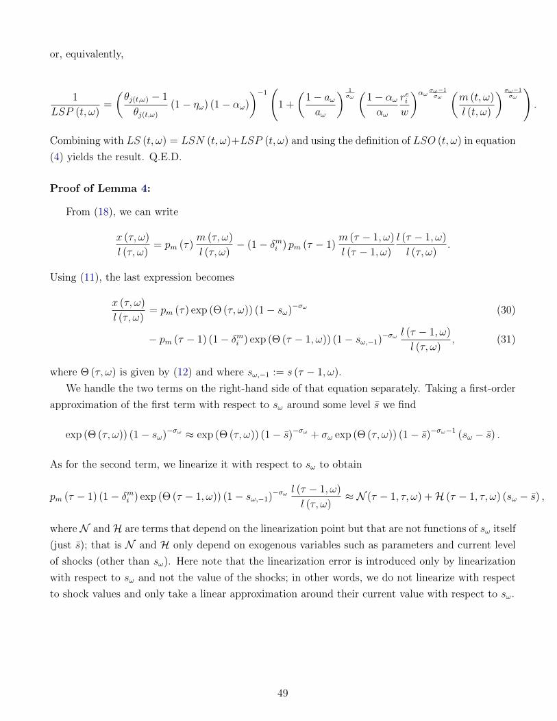
or, equivalently,
1
LSP (t, ω)=
(θj(t,ω) − 1
θj(t,ω)
(1− ηω) (1− αω)
)−1(
1 +
(1− aωaω
) 1σω(
1− αωαω
reiw
)αω σω−1σω(m (t, ω)
l (t, ω)
)σω−1σω
).
Combining with LS (t, ω) = LSN (t, ω)+LSP (t, ω) and using the definition of LSO (t, ω) in equation
(4) yields the result. Q.E.D.
Proof of Lemma 4:
From (18), we can write
x (τ, ω)
l (τ, ω)= pm (τ)
m (τ, ω)
l (τ, ω)− (1− δmi ) pm (τ − 1)
m (τ − 1, ω)
l (τ − 1, ω)
l (τ − 1, ω)
l (τ, ω).
Using (11), the last expression becomes
x (τ, ω)
l (τ, ω)= pm (τ) exp (Θ (τ, ω)) (1− sω)−σω (30)
− pm (τ − 1) (1− δmi ) exp (Θ (τ − 1, ω)) (1− sω,−1)−σωl (τ − 1, ω)
l (τ, ω), (31)
where Θ (τ, ω) is given by (12) and where sω,−1 := s (τ − 1, ω).
We handle the two terms on the right-hand side of that equation separately. Taking a first-order
approximation of the first term with respect to sω around some level s we find
exp (Θ (τ, ω)) (1− sω)−σω ≈ exp (Θ (τ, ω)) (1− s)−σω + σω exp (Θ (τ, ω)) (1− s)−σω−1 (sω − s) .
As for the second term, we linearize it with respect to sω to obtain
pm (τ − 1) (1− δmi ) exp (Θ (τ − 1, ω)) (1− sω,−1)−σωl (τ − 1, ω)
l (τ, ω)≈ N (τ − 1, τ, ω) +H (τ − 1, τ, ω) (sω − s) ,
where N andH are terms that depend on the linearization point but that are not functions of sω itself
(just s); that is N and H only depend on exogenous variables such as parameters and current level
of shocks (other than sω). Here note that the linearization error is introduced only by linearization
with respect to sω and not the value of the shocks; in other words, we do not linearize with respect
to shock values and only take a linear approximation around their current value with respect to sω.
49
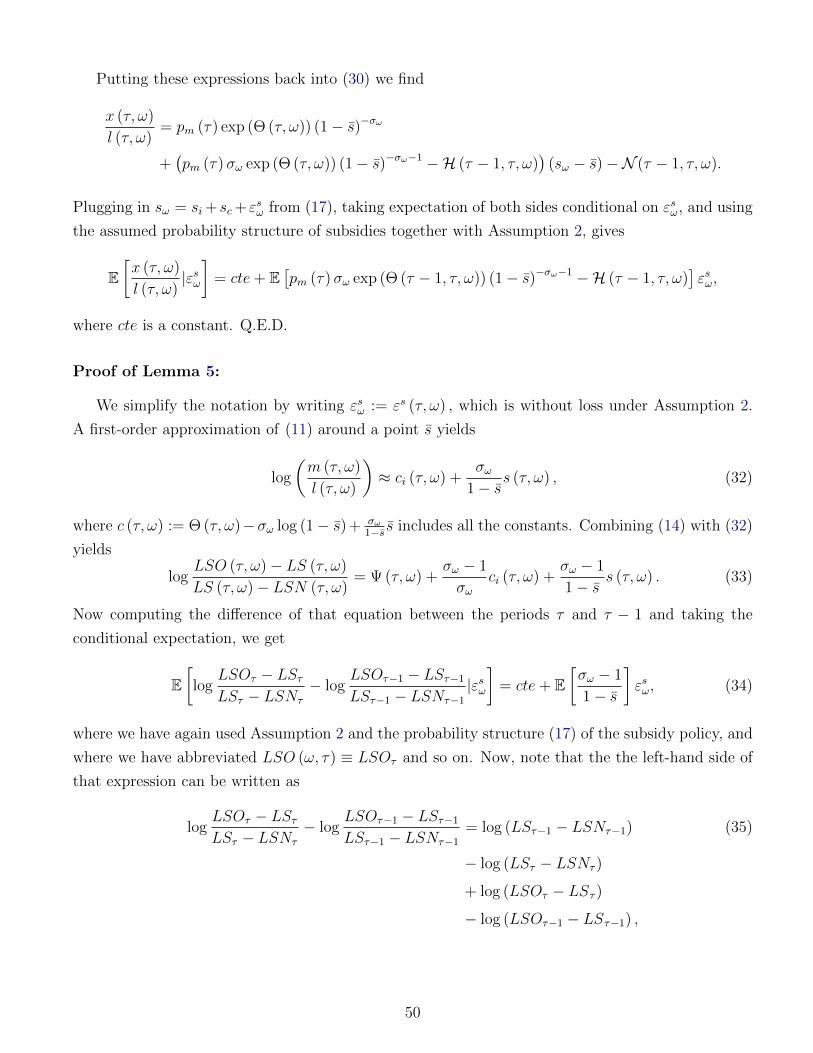
Putting these expressions back into (30) we find
x (τ, ω)
l (τ, ω)= pm (τ) exp (Θ (τ, ω)) (1− s)−σω
+(pm (τ)σω exp (Θ (τ, ω)) (1− s)−σω−1 −H (τ − 1, τ, ω)
)(sω − s)−N (τ − 1, τ, ω).
Plugging in sω = si+ sc+ εsω from (17), taking expectation of both sides conditional on εsω, and using
the assumed probability structure of subsidies together with Assumption 2, gives
E[x (τ, ω)
l (τ, ω)|εsω]
= cte+ E[pm (τ)σω exp (Θ (τ − 1, τ, ω)) (1− s)−σω−1 −H (τ − 1, τ, ω)
]εsω,
where cte is a constant. Q.E.D.
Proof of Lemma 5:
We simplify the notation by writing εsω := εs (τ, ω) , which is without loss under Assumption 2.
A first-order approximation of (11) around a point s yields
log
(m (τ, ω)
l (τ, ω)
)≈ ci (τ, ω) +
σω1− s
s (τ, ω) , (32)
where c (τ, ω) := Θ (τ, ω)−σω log (1− s) + σω1−s s includes all the constants. Combining (14) with (32)
yields
logLSO (τ, ω)− LS (τ, ω)
LS (τ, ω)− LSN (τ, ω)= Ψ (τ, ω) +
σω − 1
σωci (τ, ω) +
σω − 1
1− ss (τ, ω) . (33)
Now computing the difference of that equation between the periods τ and τ − 1 and taking the
conditional expectation, we get
E[log
LSOτ − LSτLSτ − LSNτ
− logLSOτ−1 − LSτ−1
LSτ−1 − LSNτ−1
|εsω]
= cte+ E[σω − 1
1− s
]εsω, (34)
where we have again used Assumption 2 and the probability structure (17) of the subsidy policy, and
where we have abbreviated LSO (ω, τ) ≡ LSOτ and so on. Now, note that the the left-hand side of
that expression can be written as
logLSOτ − LSτLSτ − LSNτ
− logLSOτ−1 − LSτ−1
LSτ−1 − LSNτ−1
= log (LSτ−1 − LSNτ−1) (35)
− log (LSτ − LSNτ )
+ log (LSOτ − LSτ )
− log (LSOτ−1 − LSτ−1) ,
50
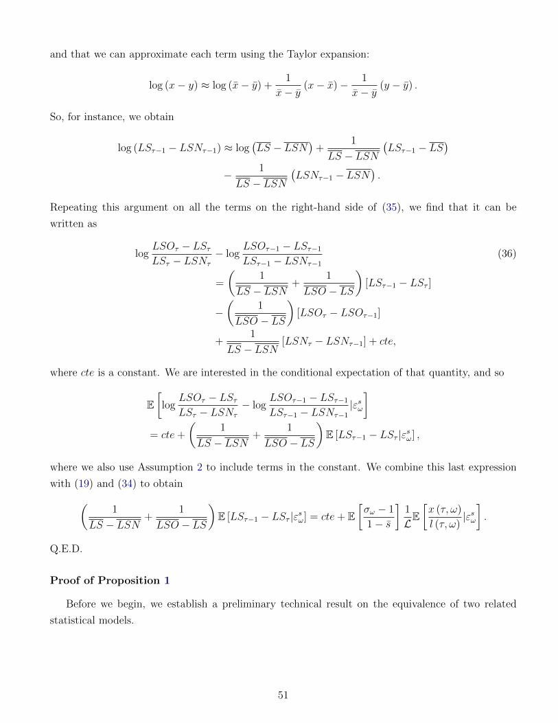
and that we can approximate each term using the Taylor expansion:
log (x− y) ≈ log (x− y) +1
x− y(x− x)− 1
x− y(y − y) .
So, for instance, we obtain
log (LSτ−1 − LSNτ−1) ≈ log(LS − LSN
)+
1
LS − LSN(LSτ−1 − LS
)− 1
LS − LSN(LSNτ−1 − LSN
).
Repeating this argument on all the terms on the right-hand side of (35), we find that it can be
written as
logLSOτ − LSτLSτ − LSNτ
− logLSOτ−1 − LSτ−1
LSτ−1 − LSNτ−1
(36)
=
(1
LS − LSN+
1
LSO − LS
)[LSτ−1 − LSτ ]
−(
1
LSO − LS
)[LSOτ − LSOτ−1]
+1
LS − LSN[LSNτ − LSNτ−1] + cte,
where cte is a constant. We are interested in the conditional expectation of that quantity, and so
E[log
LSOτ − LSτLSτ − LSNτ
− logLSOτ−1 − LSτ−1
LSτ−1 − LSNτ−1
|εsω]
= cte+
(1
LS − LSN+
1
LSO − LS
)E [LSτ−1 − LSτ |εsω] ,
where we also use Assumption 2 to include terms in the constant. We combine this last expression
with (19) and (34) to obtain(1
LS − LSN+
1
LSO − LS
)E [LSτ−1 − LSτ |εsω] = cte+ E
[σω − 1
1− s
]1
LE[x (τ, ω)
l (τ, ω)|εsω].
Q.E.D.
Proof of Proposition 1
Before we begin, we establish a preliminary technical result on the equivalence of two related
statistical models.
51

Suppose that the data-generating process is
Z = XβA + vA
X = MY V αA + uA,
where αA and βA are coefficient vectors, vA and uA are error term vectors, X and V are predetermined
matrices, and where
MY = I − PY = I − Y (Y ′Y )−1Y ′
is the orthogonal (linear) projection matrix (also known as annihilator matrix) that returns residual
from projecting any conformable matrix on the subspace generated by Y (a predetermined variable).
PY is the (linear) projection matrix that returns predicted values (also known as prediction matrix).
We will refer to this system of equations as model A.
Consider an alternative model (model B) that follows the equations
Z = XβB + Y γB + vB
X = V αB + Y δB + uB,
where αB, βB, δB and γB are coefficient vectors and vB and uB are error term vectors that are
orthogonal to Y in the sense that MY vB = MY uB = 0. Note that the above definition implies that
the error terms are related as follows:
XβA + vA = XβB + Y γB + vB
and
V αB + Y δB + uB = MY V αA + uA,
which after multiplying both sides by the orthogonal projection matrix MY implies
MY V αB +MY uB = MY V αA +MY uA. (37)
The parameters for model A and model B are identical and their estimates have identical prop-
erties, as stated in the lemma below.
Lemma 6. The two-stage least squares estimators of model A and model B yield the same point
estimates for βA and βB and for αA and αB, and these estimators have the same variance.
The proof of this fact is a straightforward corollary of a standard result in econometrics: the
Frisch–Waugh–Lovell theorem. Since it is standard and technical, we relegate it to the Technical
Appendix.
52
The proof of the Proposition 1 now trivially follows from Lemma (4) and Lemma (5) and the
basic properties of a conditional expectations operator, i.e., the fact that for any random variable X
and Y (with bounded expectation) we have Y = E [Y |X] + ε, we know 1) E [ε|X] = 0, 2) E [ε] = 0,
3) for any function h(X) such that E [|h(X)ε|] < ∞, E [h(X)ε] = 0. It is clear that the first stage
boils down to model A. Under the independence assumption the terms si, sc are random variables
that can be estimated by a fixed effect regression of the form s = FEc + FEi + ε (see Wooldridge
(2001), section 10.2.1). This is equivalent to estimating model B as stated in the proposition by the
above lemma. Detailed proof can be found in the Technical Appendix. Q.E.D.
D Robustness to correlated pre-existing subsidies
In this section, we generalize the theoretical results of Section 1 to allow for a pre-existing subsidy
for automation investment in the period τ − 1, which would have violated Assumption 2. More
specifically, we assume that the part of subsidies s (τ, ω) and s (τ − 1, ω) that are orthogonal to the
industry and city variables are related as follows:
εs (τ − 1, ω) = ρsωεs (τ, ω) + vsω, (38)
where ρsω and vsω are i.i.d. shocks with mean 0. The results that are affected by this change are Lemma
4, Lemma 5 and Proposition 1. Since modifying the proofs is fairly straightforward we relegate the
proofs to the Technical Appendix. The resulting statement of the proposition is identical. The only
difference is that the constant B that is carried around is given by
B = − 1
1− s1
L
(1
LS − LSN+
1
LSO − LS
)−1
E [(σω − 1) (1− ρsω)] , (39)
instead of by (21).
Implications for estimating the average elasticity E [σω]
We now show that the above modification implies that, when 0 < E [ρsω], our estimated elasticity
is biased toward a smaller E [σω] and, as a result, against finding a large effect of automation on the
labor share. To see this, note that we can find E [σω] by using the estimated coefficients B and L.
Namely, from (39) we can write
E [σω − 1] = −LB 1− sE [1− ρsω]
(1
LS − LSN+
1
LSO − LS
)(40)
where we have used the fact that ρsω is independent of other random variables. It is clear that the
right-hand side of (40) is an increasing function of E [ρsω] (the product LB is always negative in our
estimates and 1− s, LS − LSN and LSO − LS are positive by the restrictions of the model). As a
53

result, by assuming that E [ρsω] = 0 as in our benchmark exercises, we would be biasing our estimate
toward a smaller E [σω].
54