the flutter shutter - image...
TRANSCRIPT

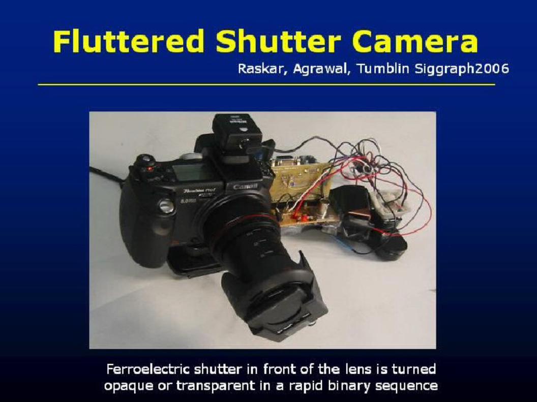
The Flutter Shutter
Overview
● The Fourier transform and the sinc function ● Poisson random variable● Steady acquisition model● Fundamental principle of photography● The Raskar Flutter Shutter● Acquisition model of a moving landscape● The numerical Flutter Shutter● The Flutter Shutter paradox
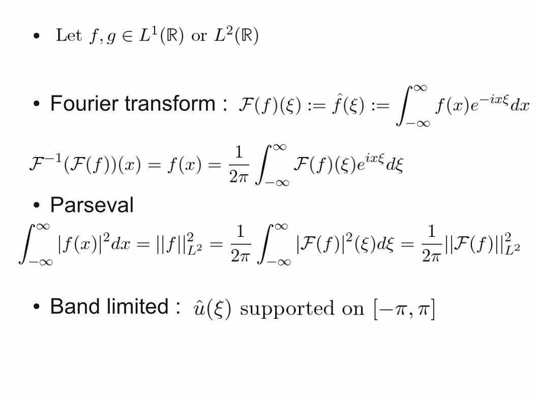
●
● Fourier transform :
● Parseval
● Band limited :
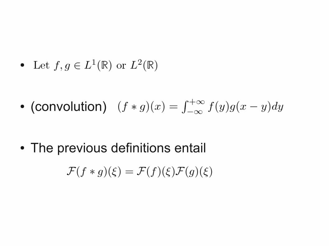
●
● (convolution)
● The previous definitions entail
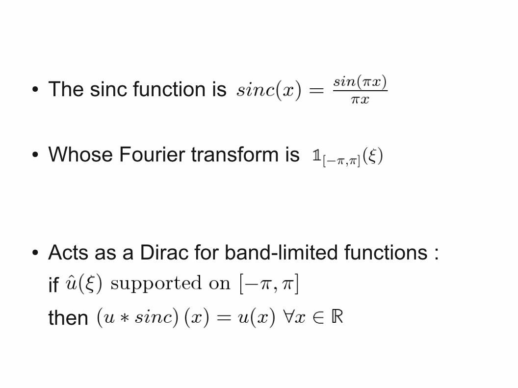
● The sinc function is
● Whose Fourier transform is
● Acts as a Dirac for band-limited functions :
if
then
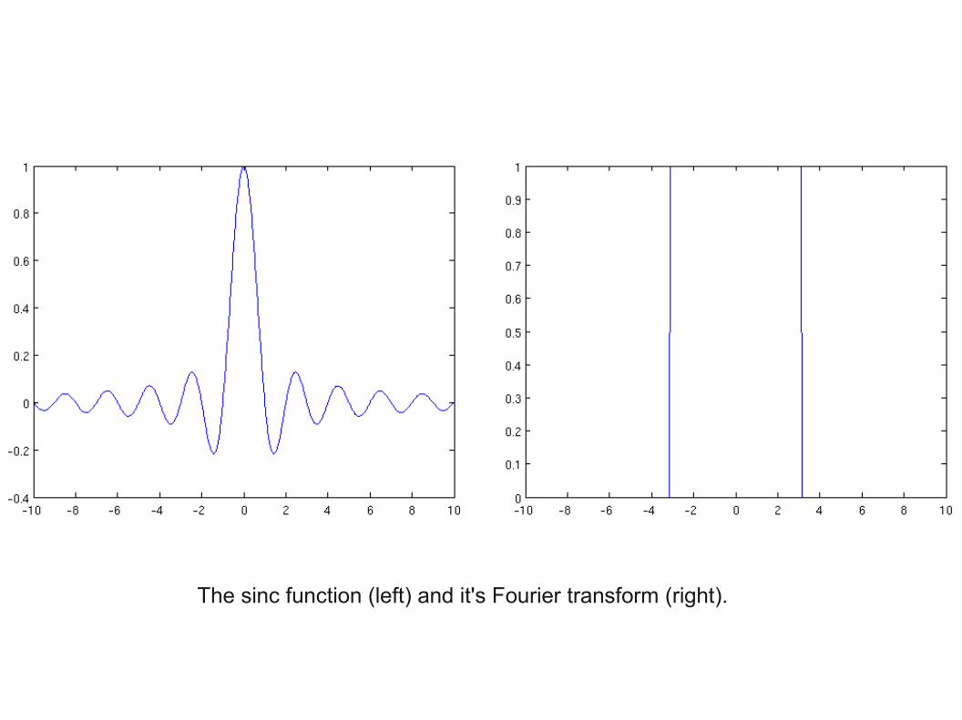
The sinc function (left) and it's Fourier transform (right).
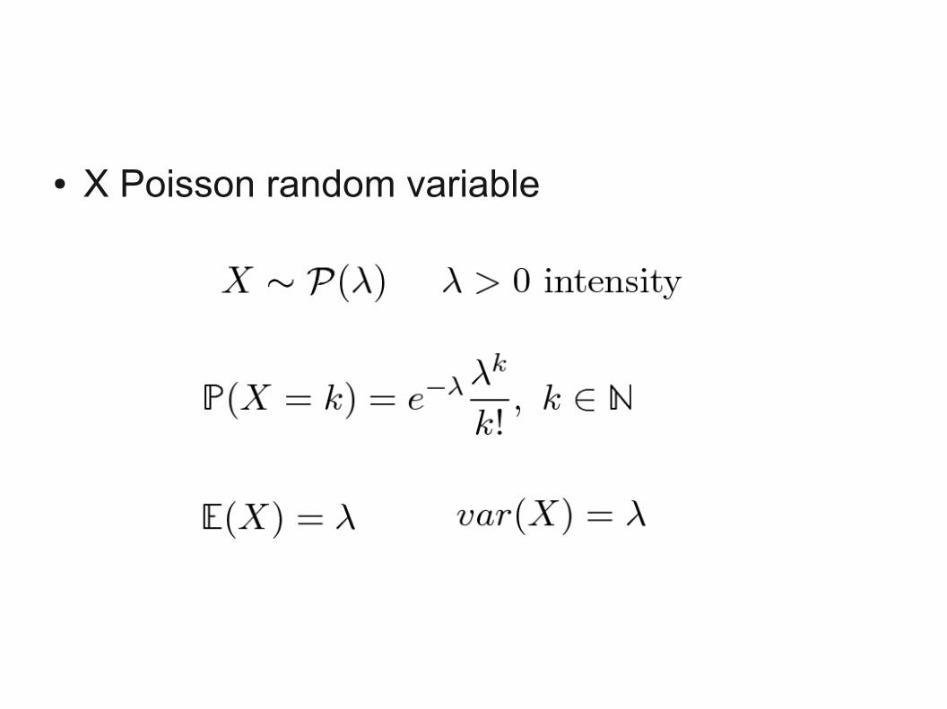
● X Poisson random variable
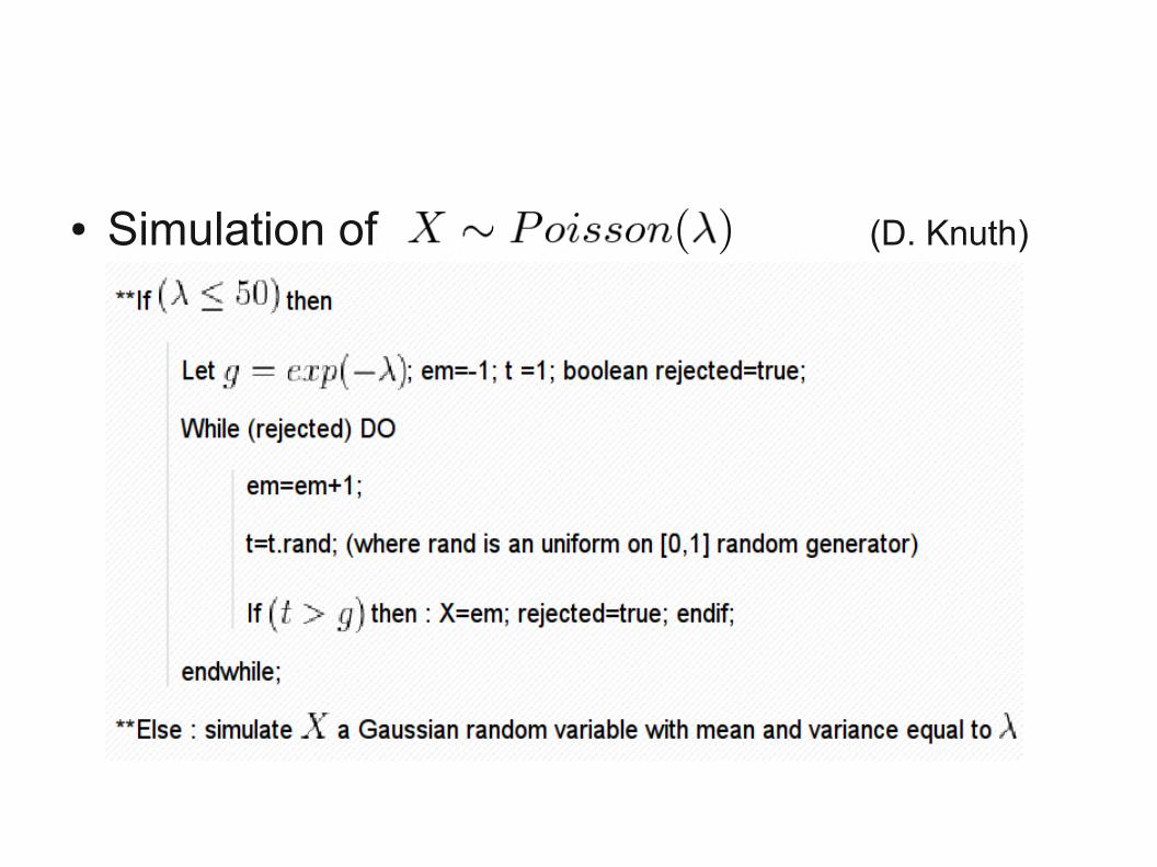
● Simulation of (D. Knuth)
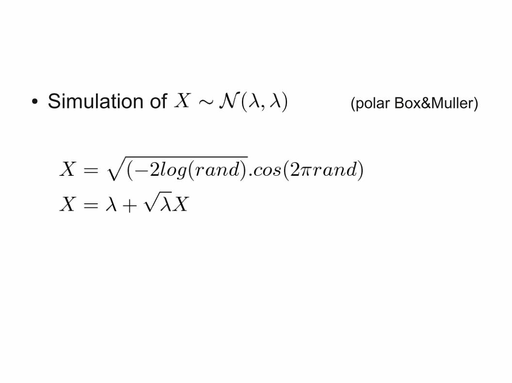
● Simulation of (polar Box&Muller)
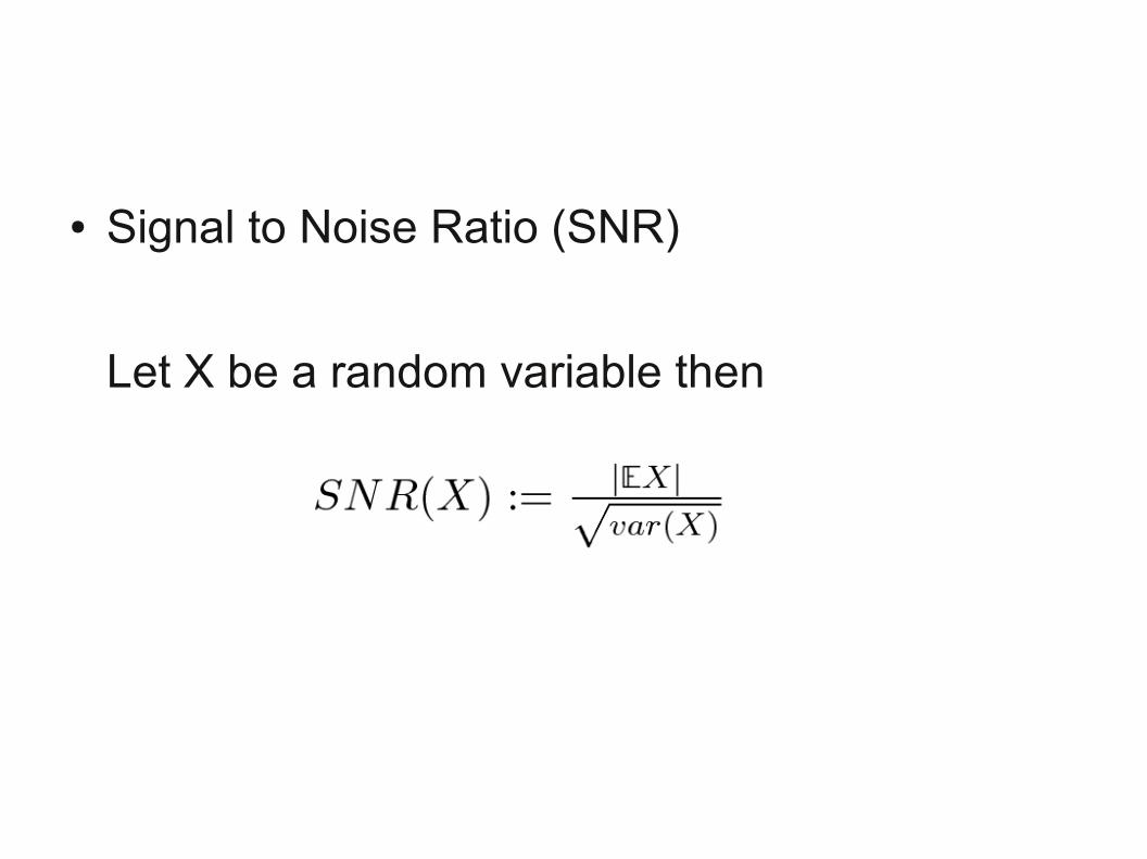
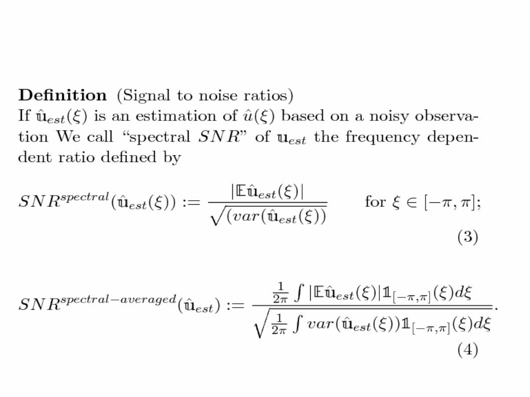
● Signal to Noise Ratio (SNR)
Let X be a random variable then
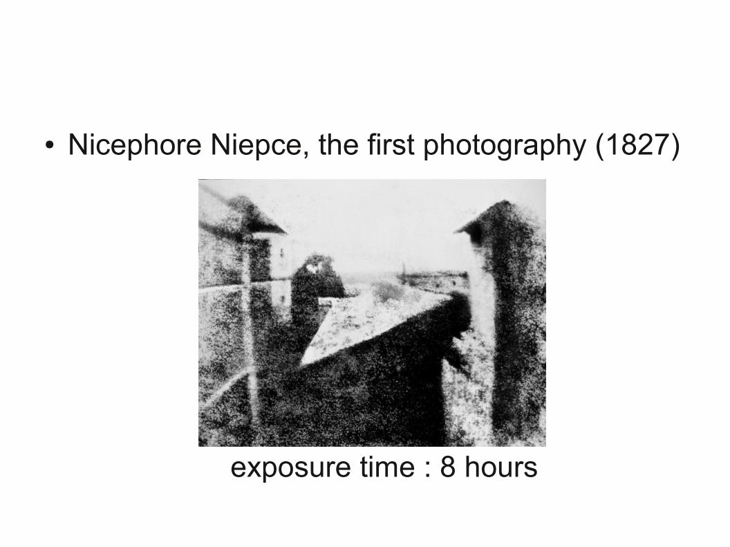
● Nicephore Niepce, the first photography (1827)
exposure time : 8 hours
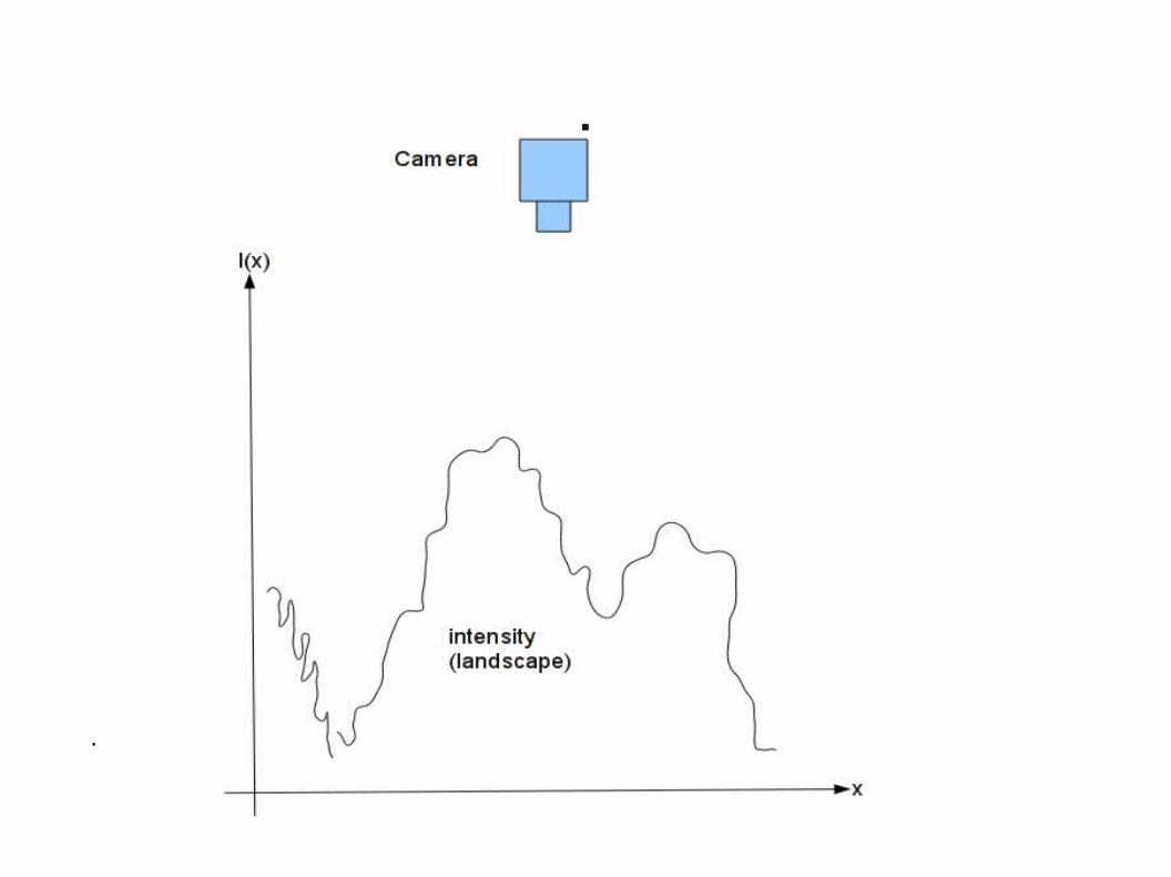
● Acquisition model (1D setting)
Real (non observable) landscape :
(deterministic intensity field)
which represents the photon emission at time and position
.
.
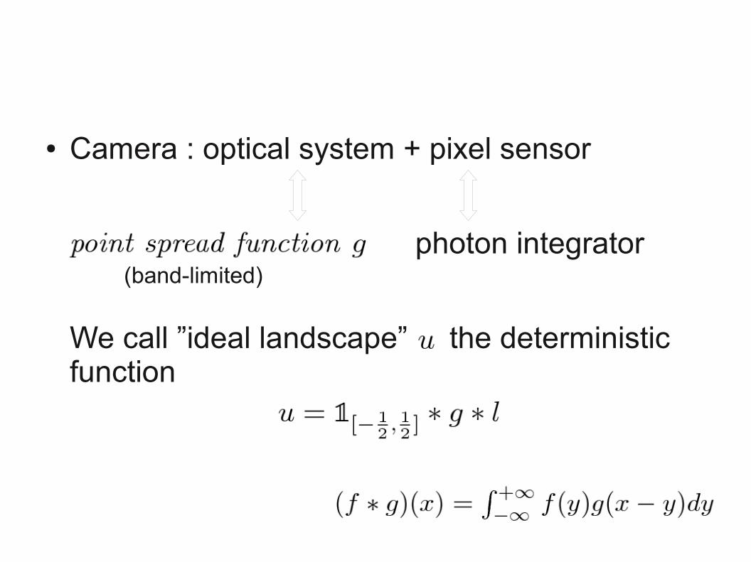
● Camera : optical system + pixel sensor
photon integrator
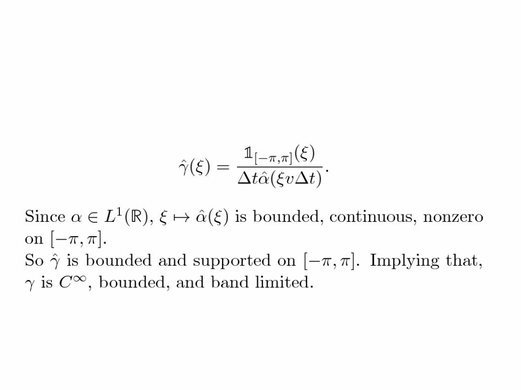
We call ”ideal landscape” the deterministic function
(band-limited)
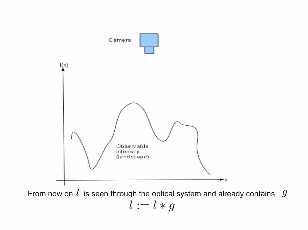
From now on is seen through the optical system and already contains
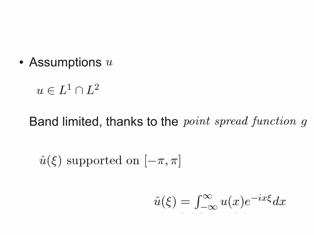
● Assumptions
Band limited, thanks to the
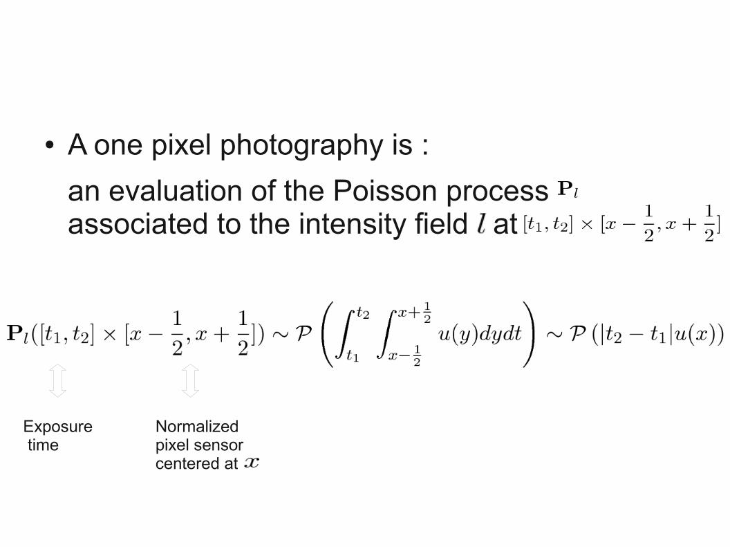
Exposure time
Normalized pixel sensor centered at
● A one pixel photography is :
an evaluation of the Poisson process associated to the intensity field at
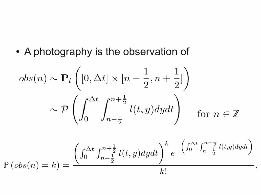
● A photography is the observation of

● The pixel sensors are disjoint
are in independent Poisson random variables
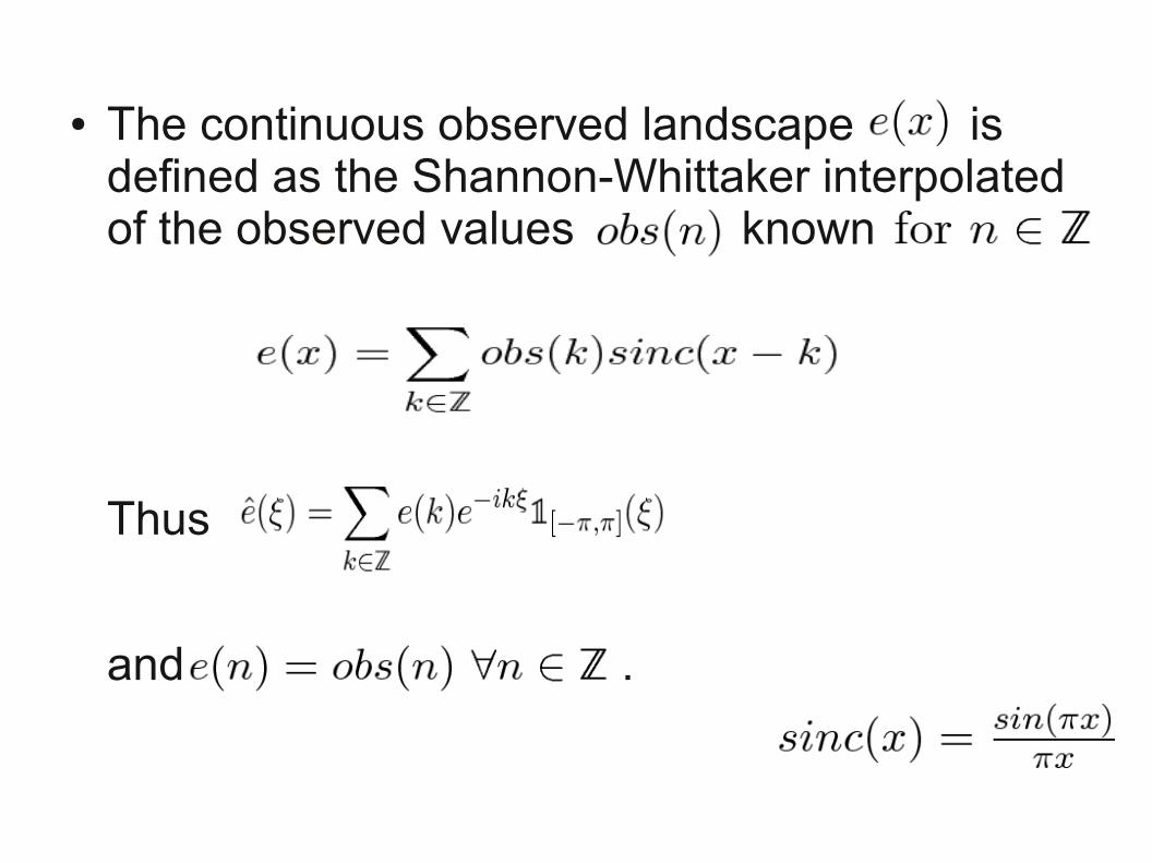
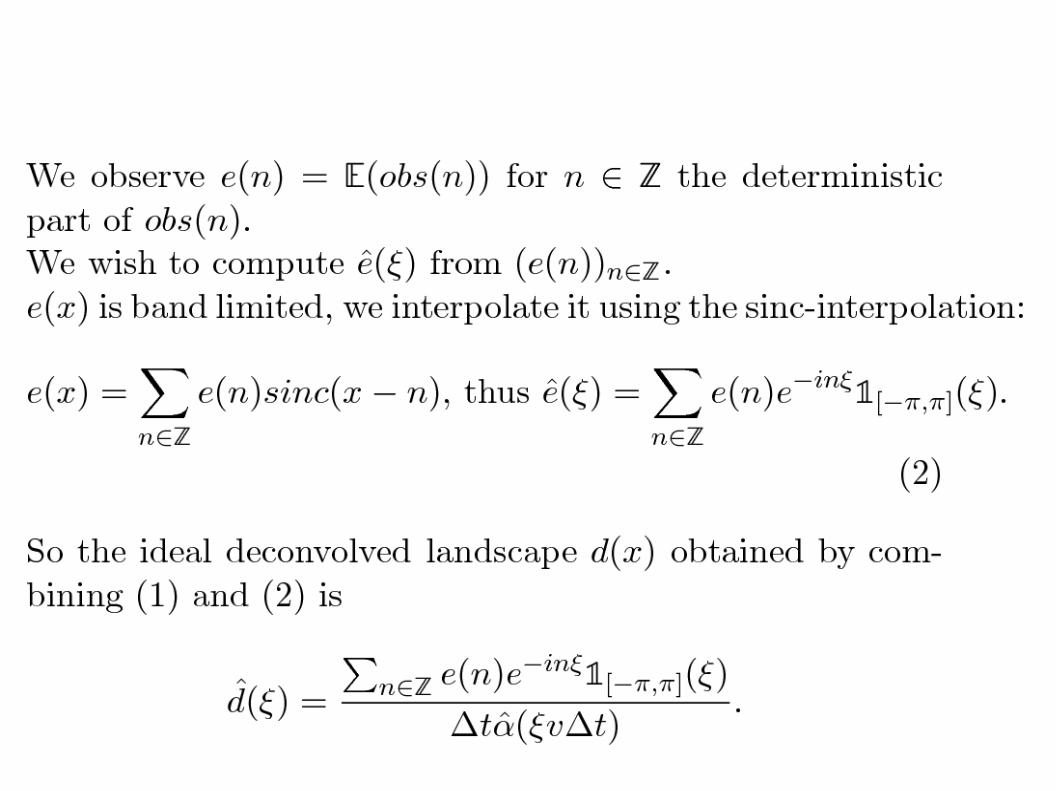
● The continuous observed landscape is defined as the Shannon-Whittaker interpolated of the observed values known
Thus
and .
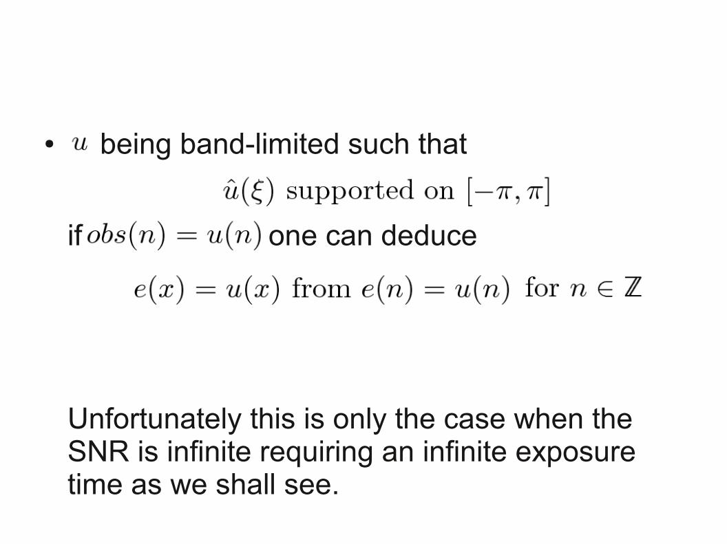
● being band-limited such that
if one can deduce
Unfortunately this is only the case when the SNR is infinite requiring an infinite exposure time as we shall see.
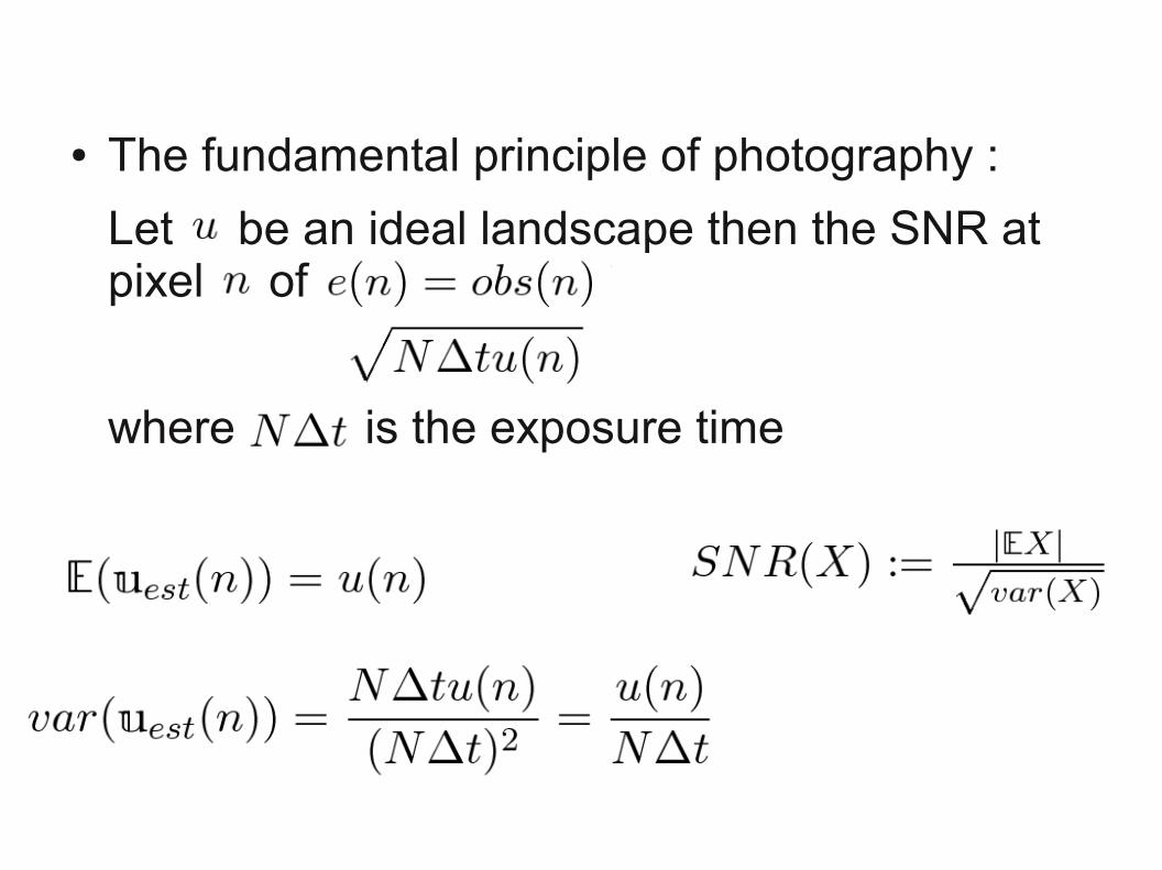
● The fundamental principle of photography :
Let be an ideal landscape then the SNR at pixel of
where is the exposure time
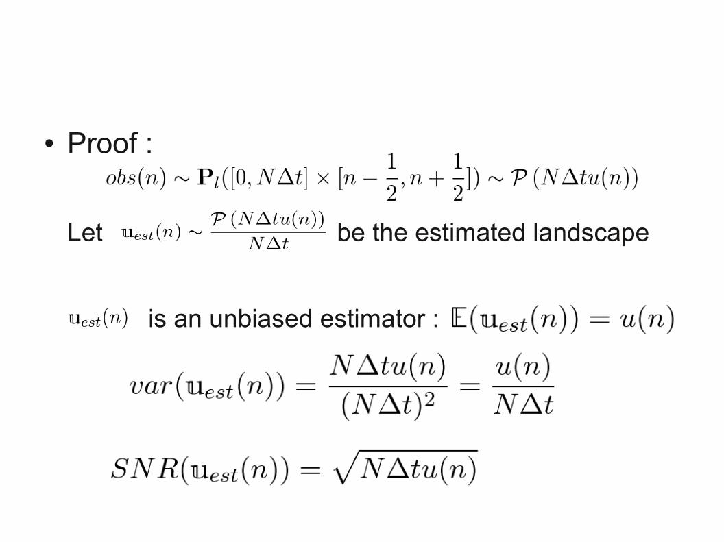
● Proof :
Let be the estimated landscape
is an unbiased estimator :
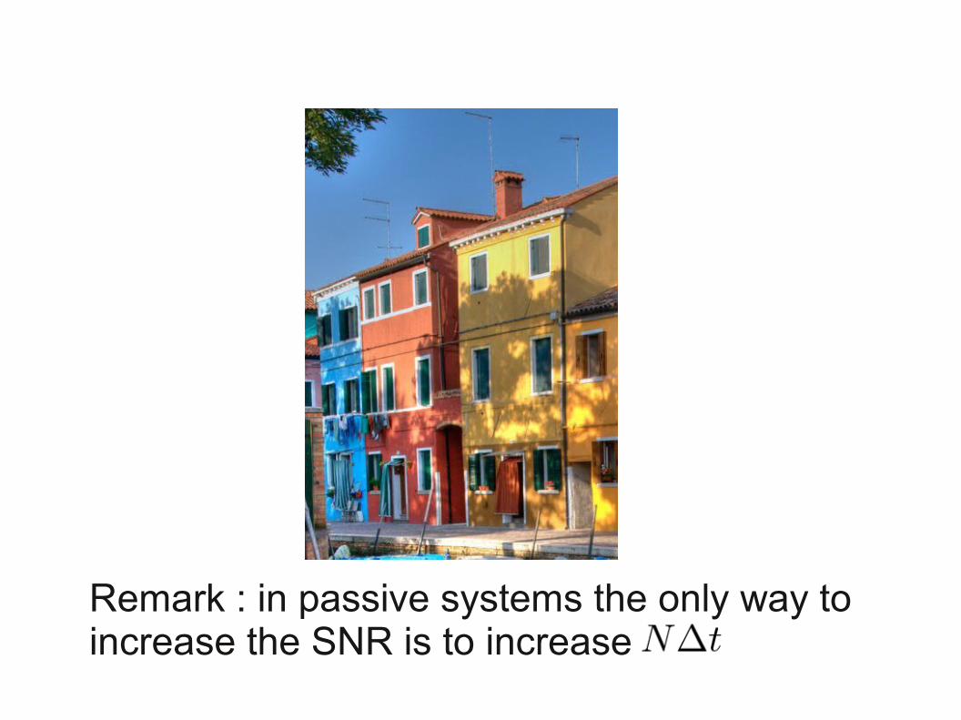
Remark : in passive systems the only way to increase the SNR is to increase

Exposure time= , SNR=100, numbers of photons (average) : .
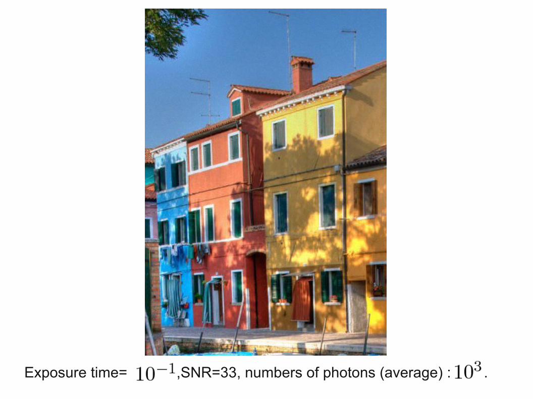
Exposure time= ,SNR=33, numbers of photons (average) : .

Exposure time= , SNR=10, numbers of photons (average) : .
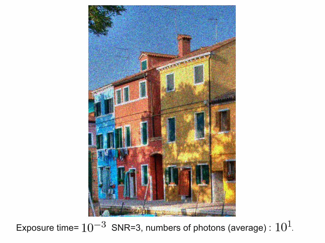
Exposure time= , SNR=3, numbers of photons (average) : .
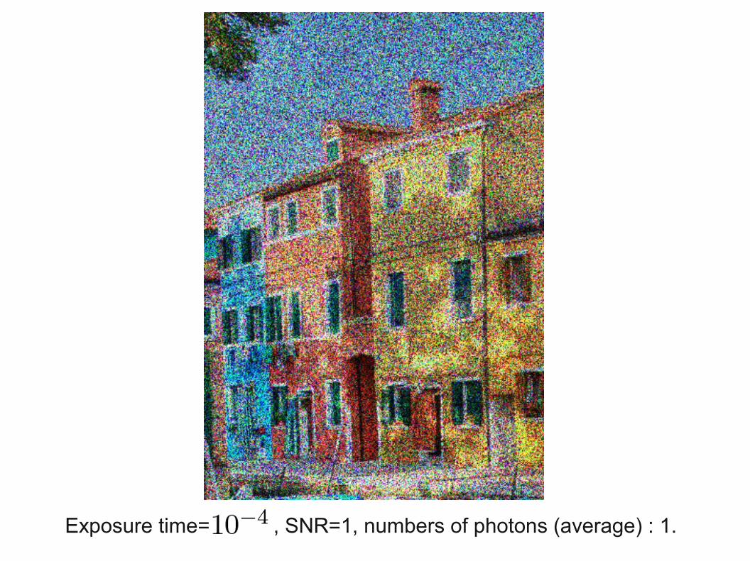
Exposure time= , SNR=1, numbers of photons (average) : 1.
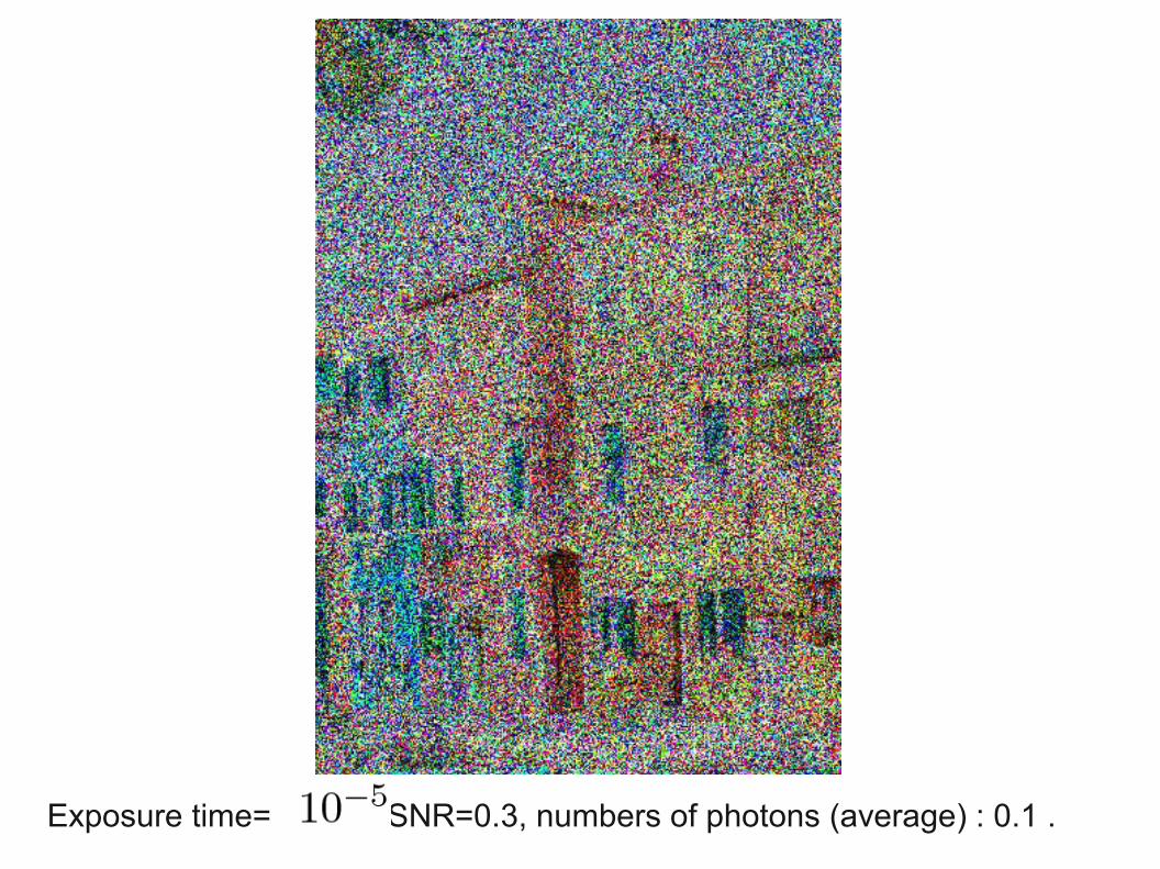
Exposure time= , SNR=0.3, numbers of photons (average) : 0.1 .
Moving camera
Observable intensity(landscape)
l(x)
x
v
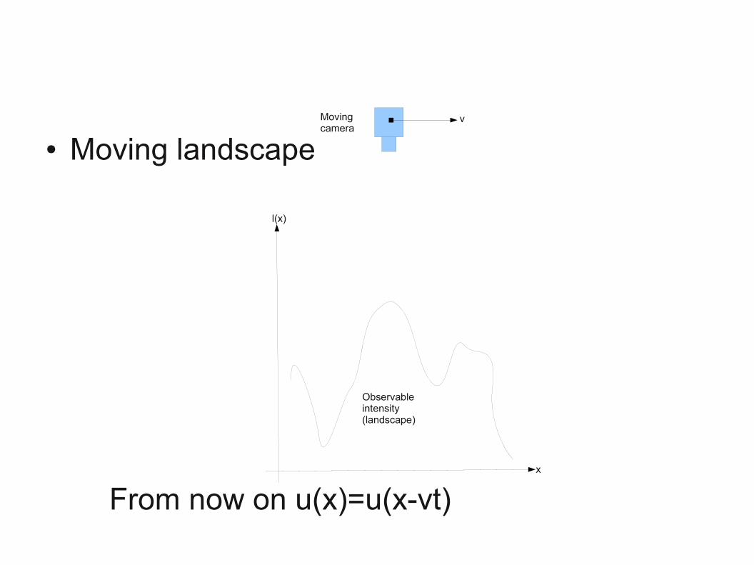
● Moving landscape
From now on u(x)=u(x-vt)
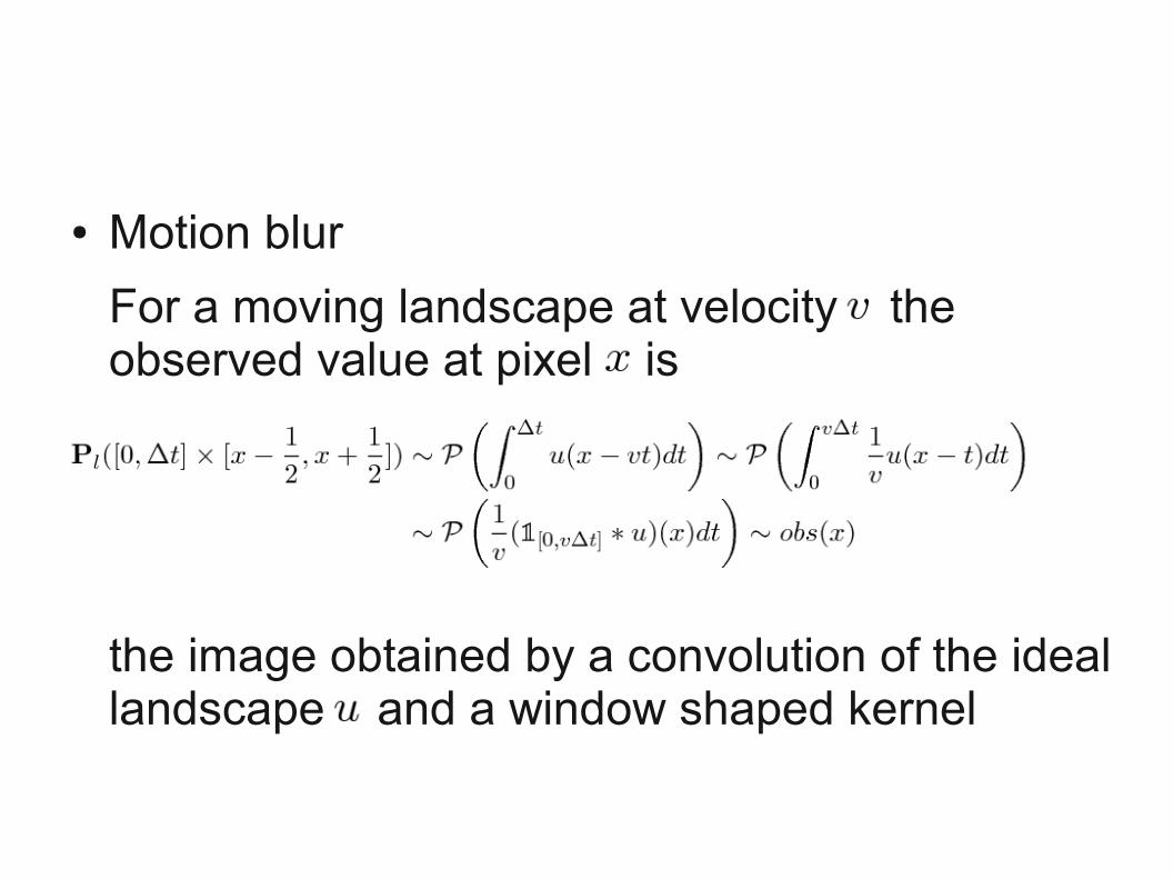
● Motion blur
For a moving landscape at velocity the observed value at pixel is
the image obtained by a convolution of the ideal landscape and a window shaped kernel
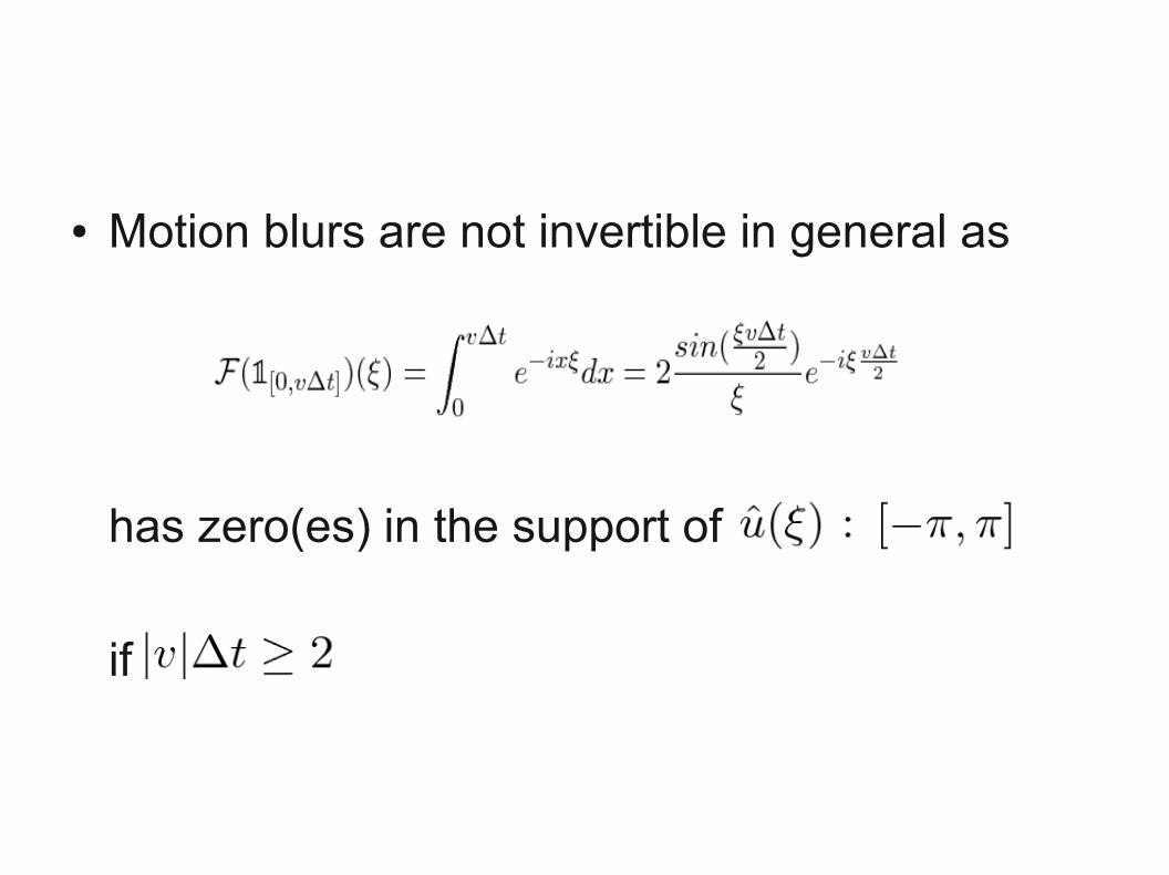
● Motion blurs are not invertible in general as
has zero(es) in the support of
if
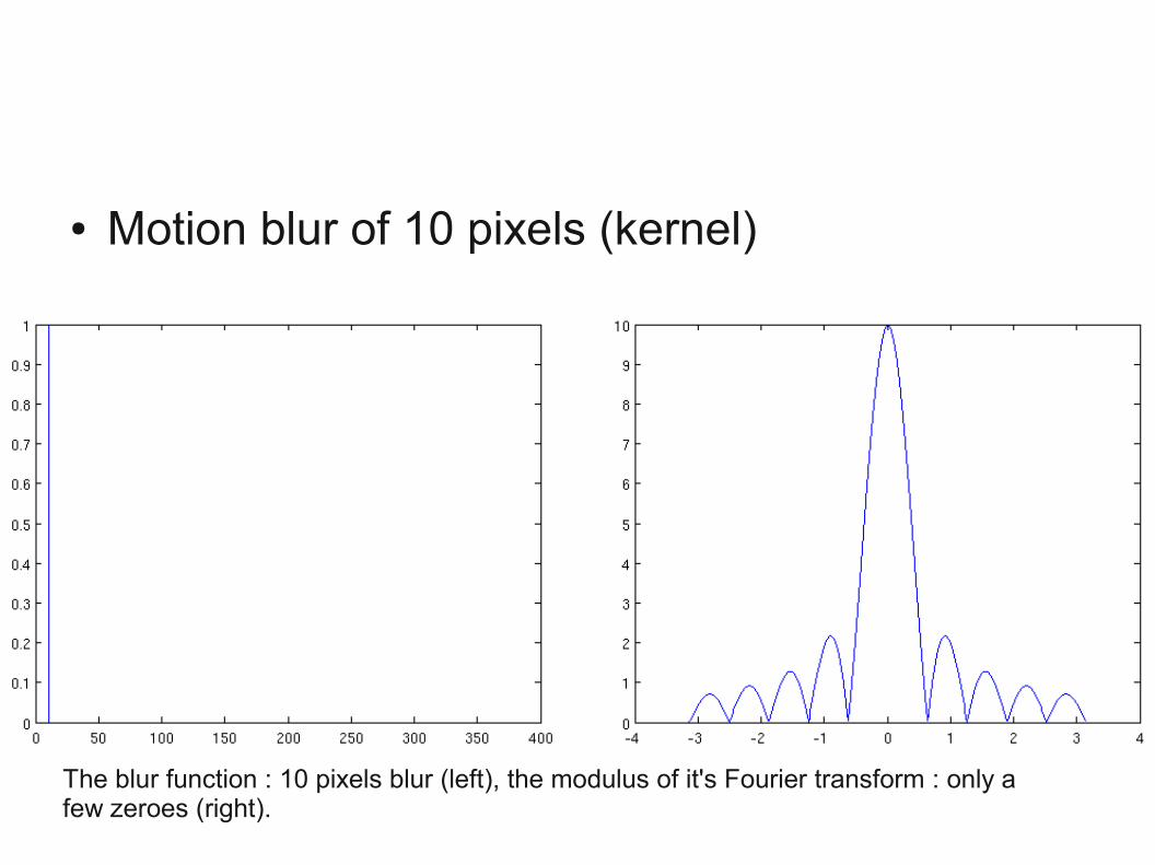
● Motion blur of 10 pixels (kernel)
The blur function : 10 pixels blur (left), the modulus of it's Fourier transform : only a few zeroes (right).
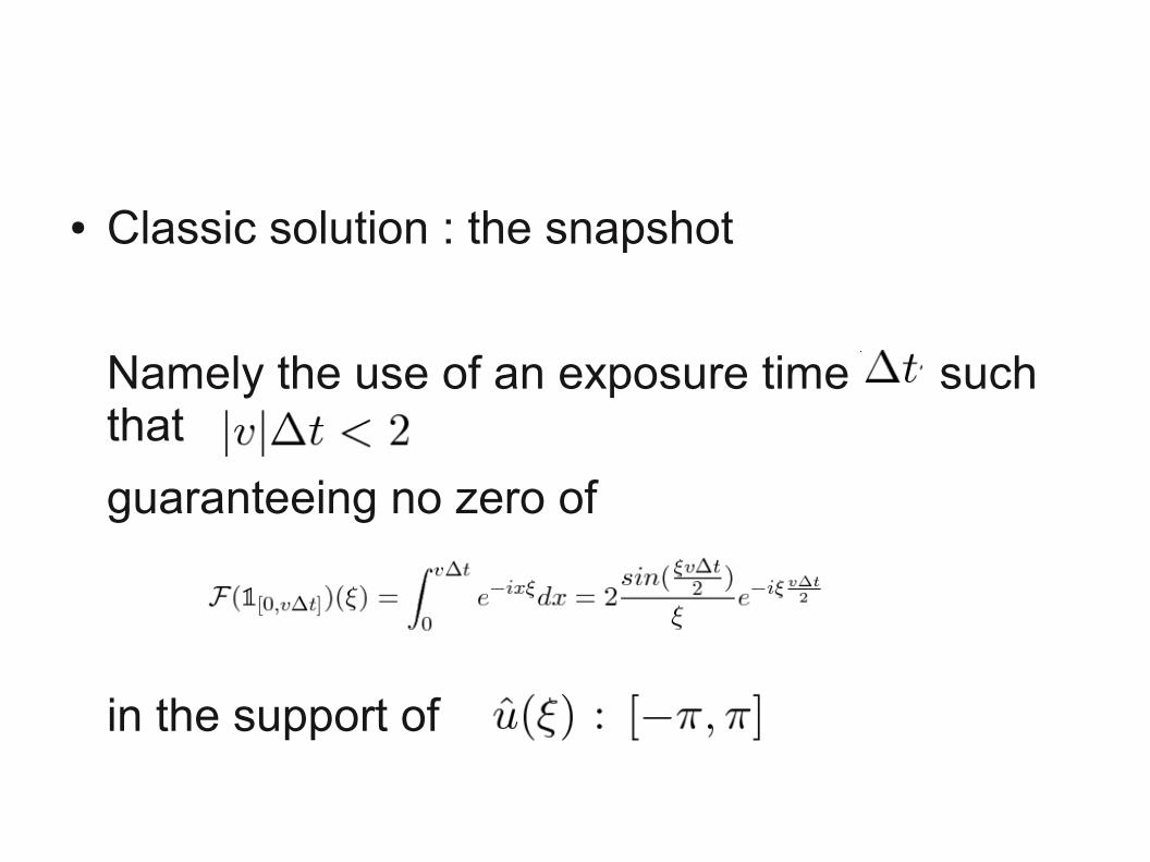
● Classic solution : the snapshot
Namely the use of an exposure time such that
guaranteeing no zero of
in the support of
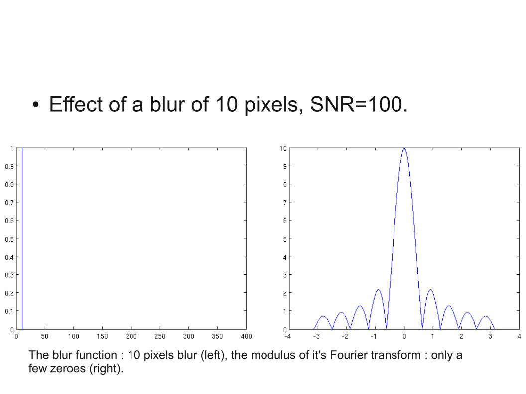
● Effect of a blur of 10 pixels, SNR=100.
The blur function : 10 pixels blur (left), the modulus of it's Fourier transform : only a few zeroes (right).
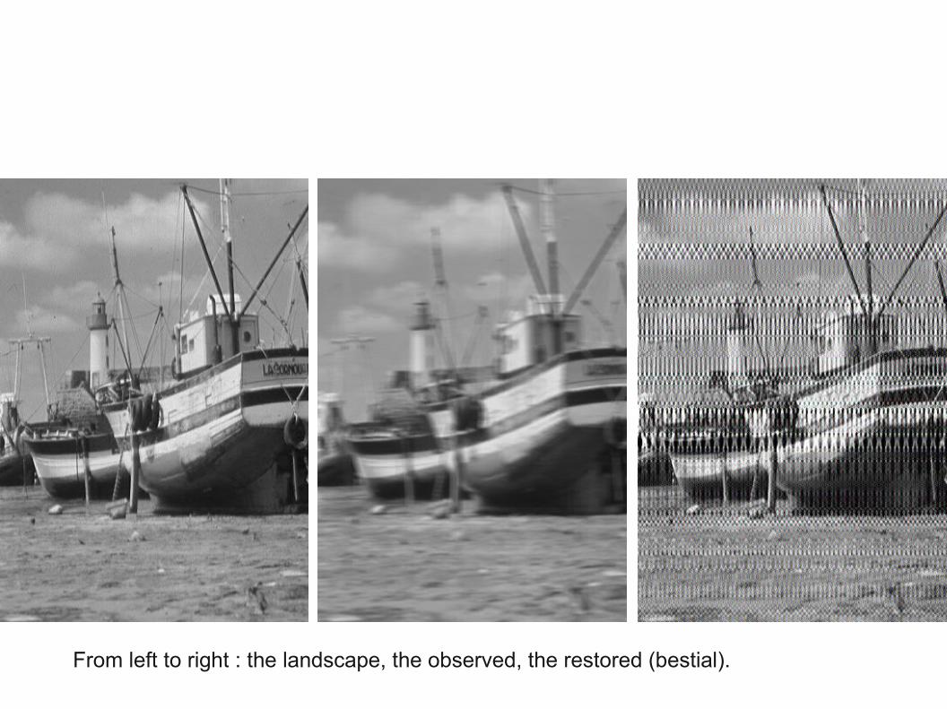
From left to right : the landscape, the observed, the restored (bestial).
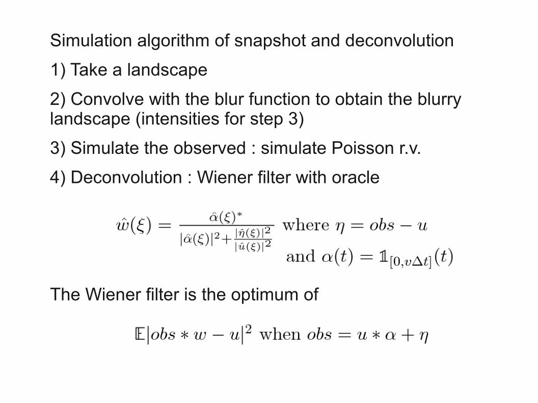
Simulation algorithm of snapshot and deconvolution
1) Take a landscape
2) Convolve with the blur function to obtain the blurry landscape (intensities for step 3)
3) Simulate the observed : simulate Poisson r.v.
4) Deconvolution : Wiener filter with oracle
The Wiener filter is the optimum of
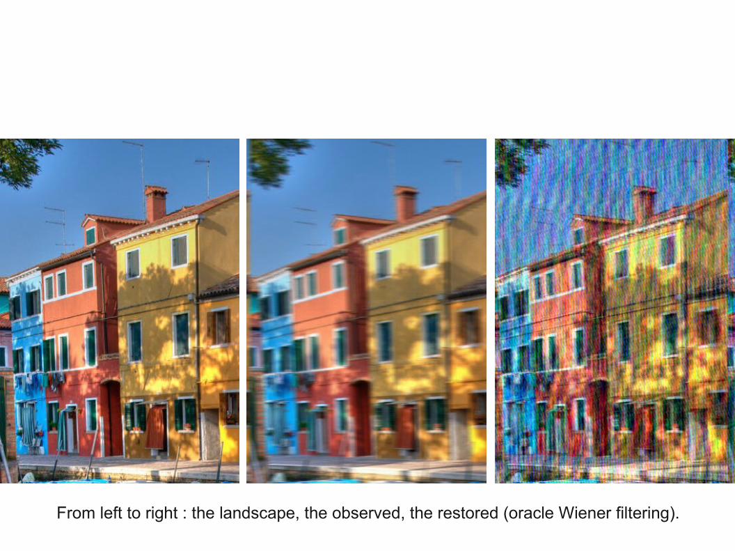
From left to right : the landscape, the observed, the restored (oracle Wiener filtering).
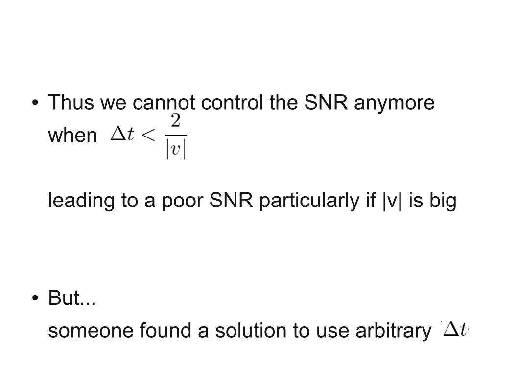
● Thus we cannot control the SNR anymore
when
leading to a poor SNR particularly if |v| is big
● But...
someone found a solution to use arbitrary

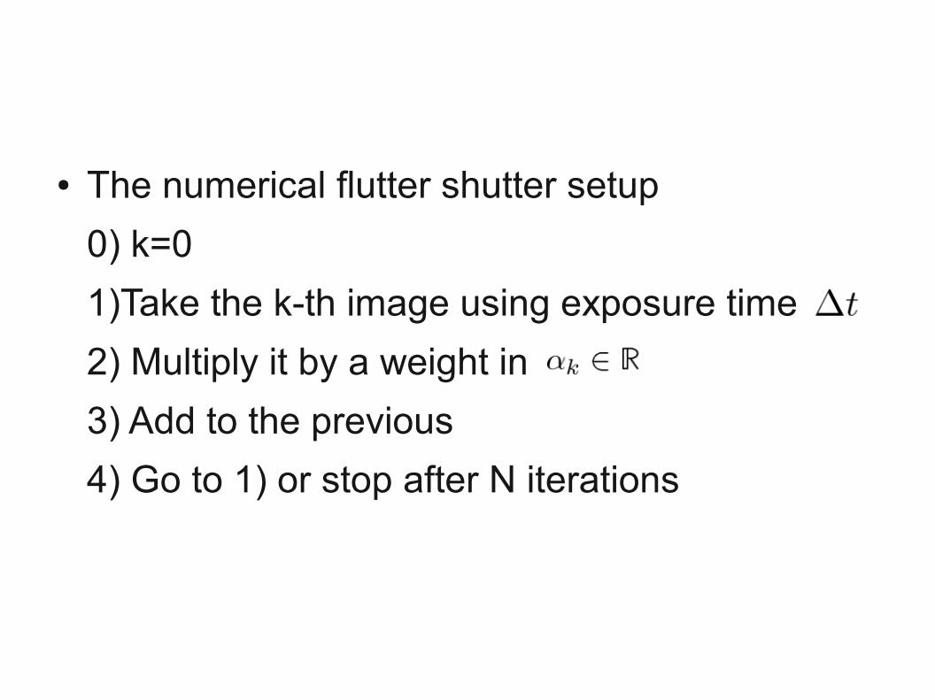
● The numerical flutter shutter setup
0) k=0
1)Take the k-th image using exposure time
2) Multiply it by a weight in
3) Add to the previous
4) Go to 1) or stop after N iterations
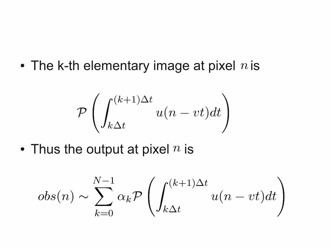
● The k-th elementary image at pixel is
● Thus the output at pixel is
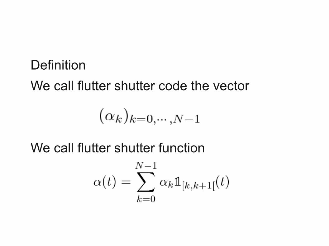
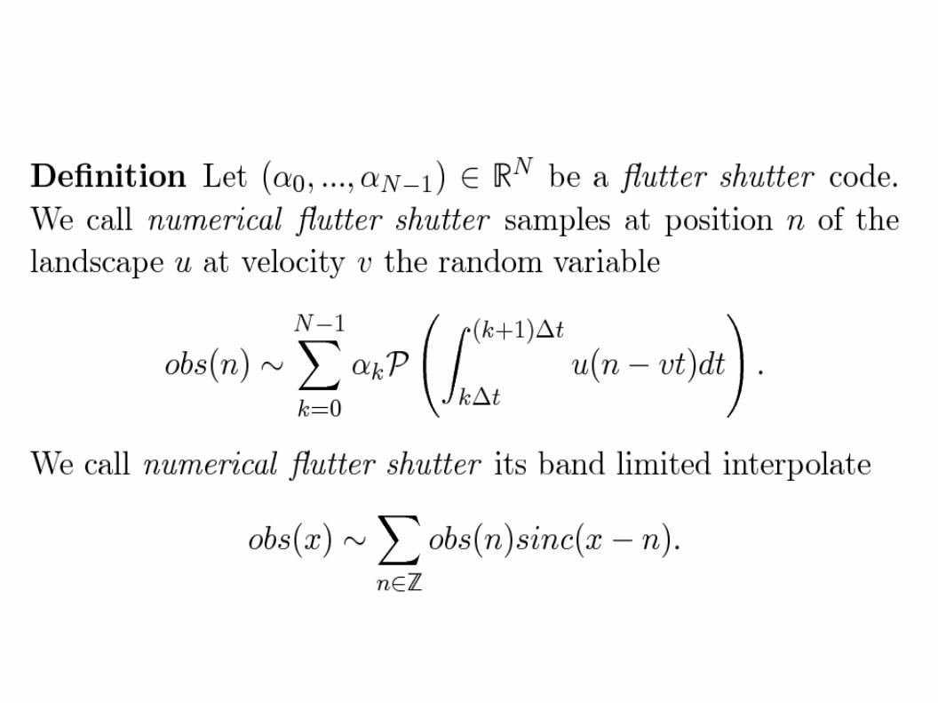
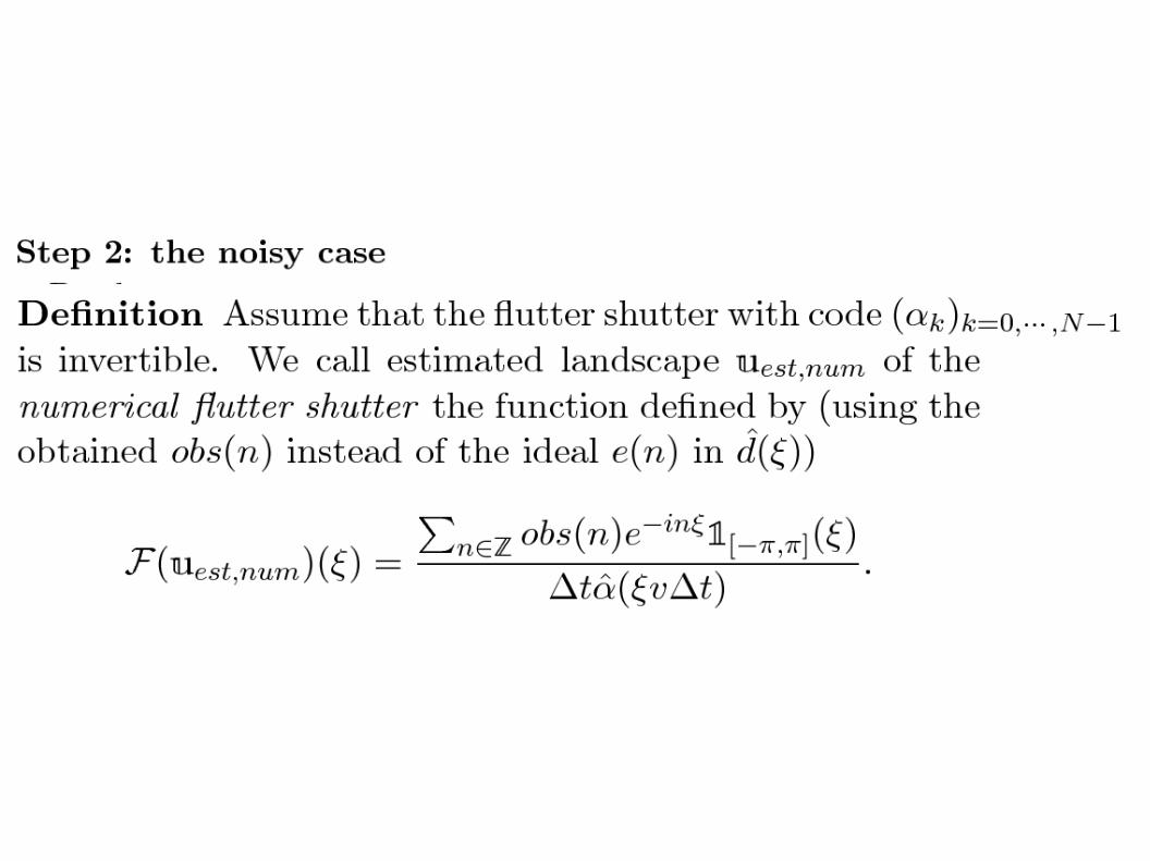
Definition
We call flutter shutter code the vector
We call flutter shutter function
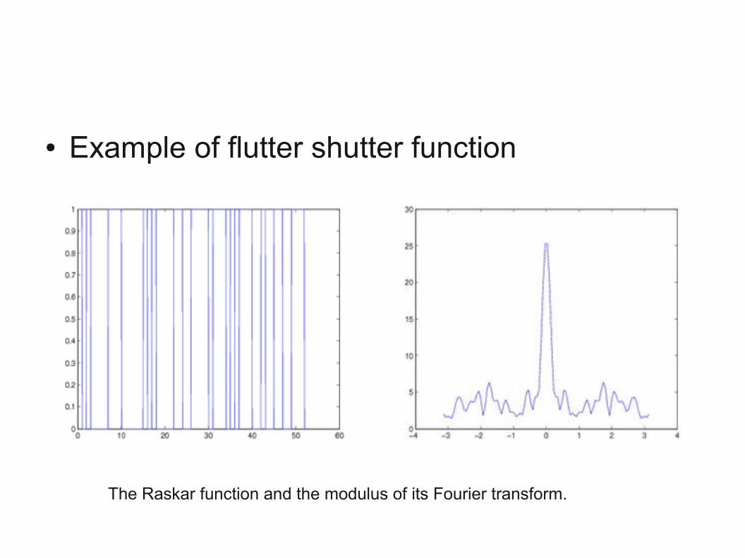
● Example of flutter shutter function
The Raskar function and the modulus of its Fourier transform.
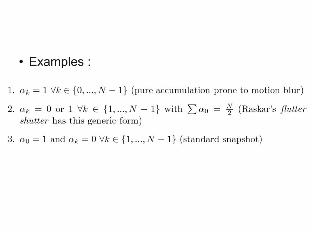
● Examples :
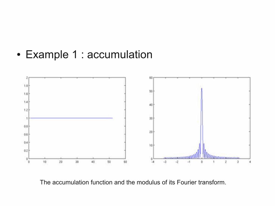
● Example 1 : accumulation
The accumulation function and the modulus of its Fourier transform.

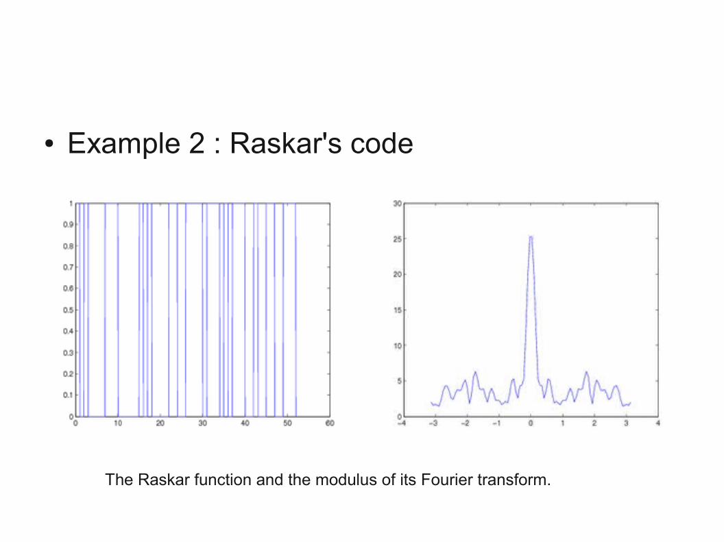
● Example 2 : Raskar's code
The Raskar function and the modulus of its Fourier transform.
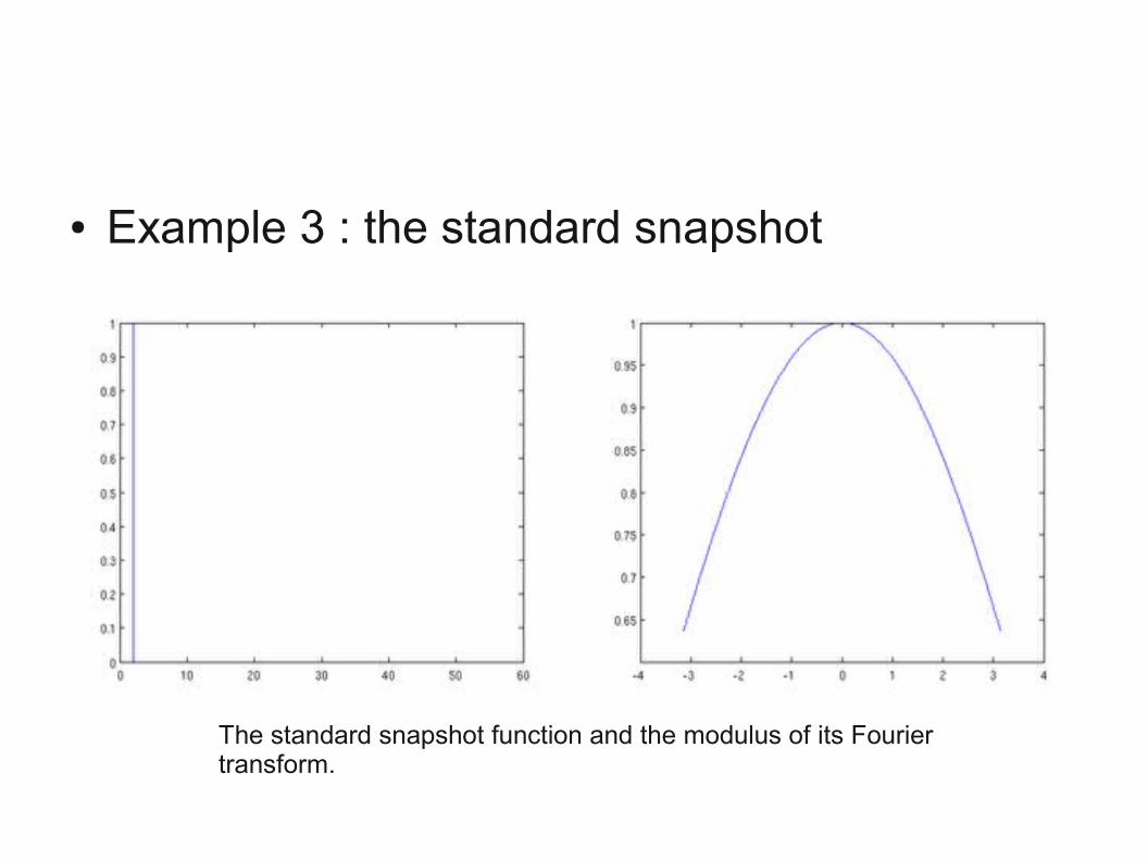
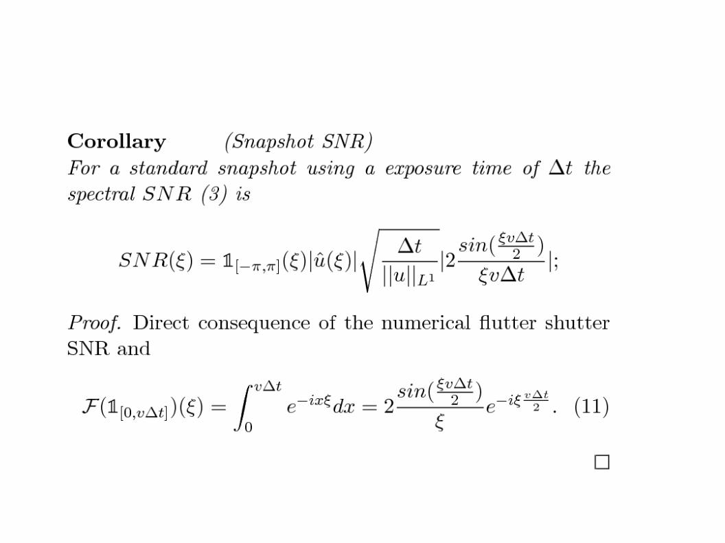
● Example 3 : the standard snapshot
The standard snapshot function and the modulus of its Fourier transform.
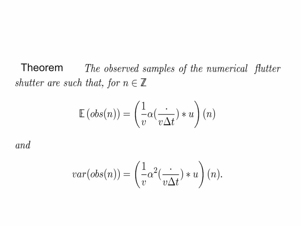
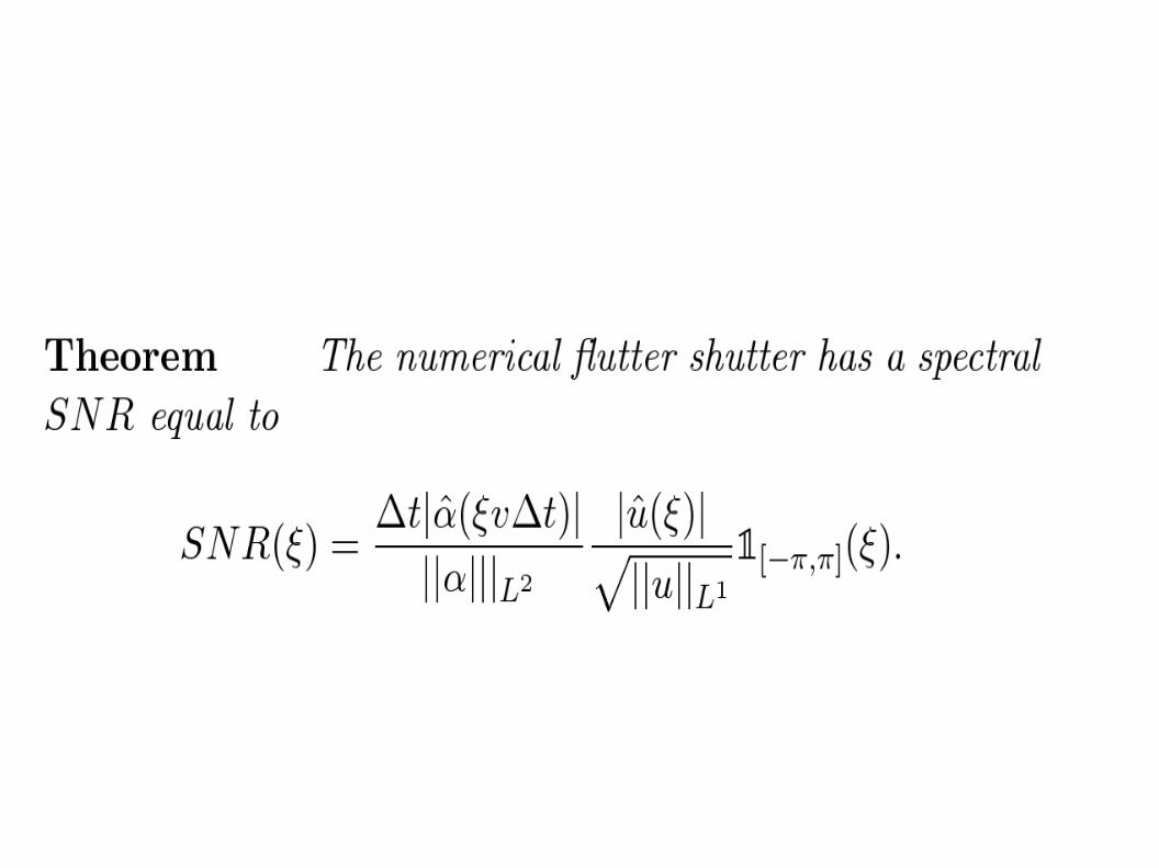
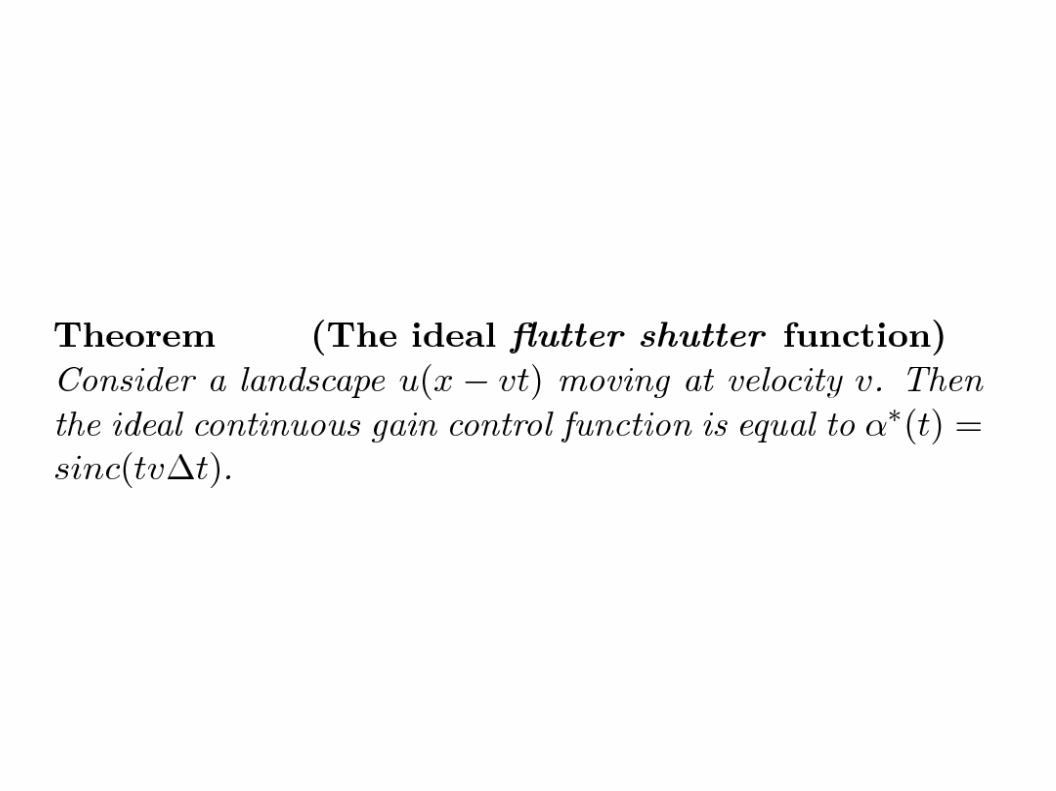
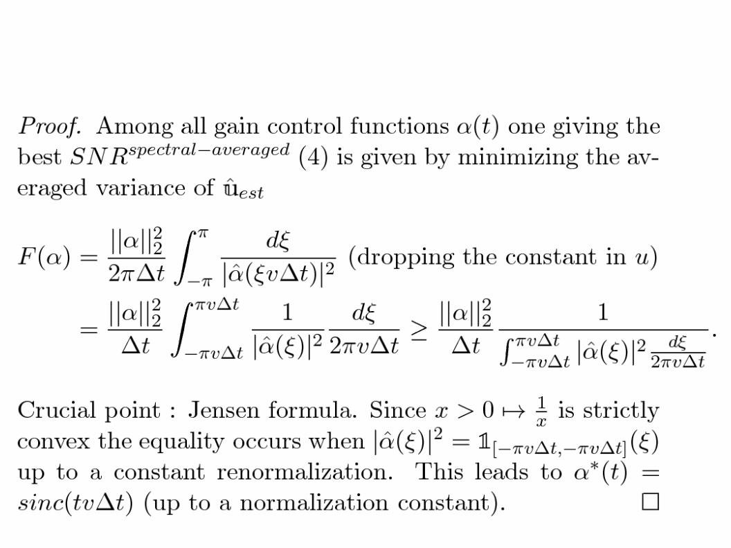
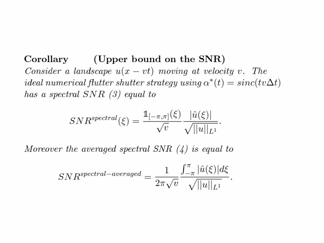
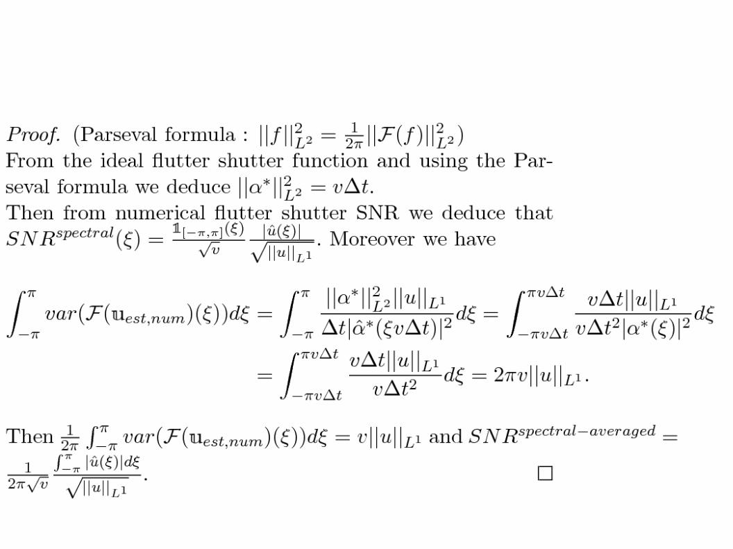
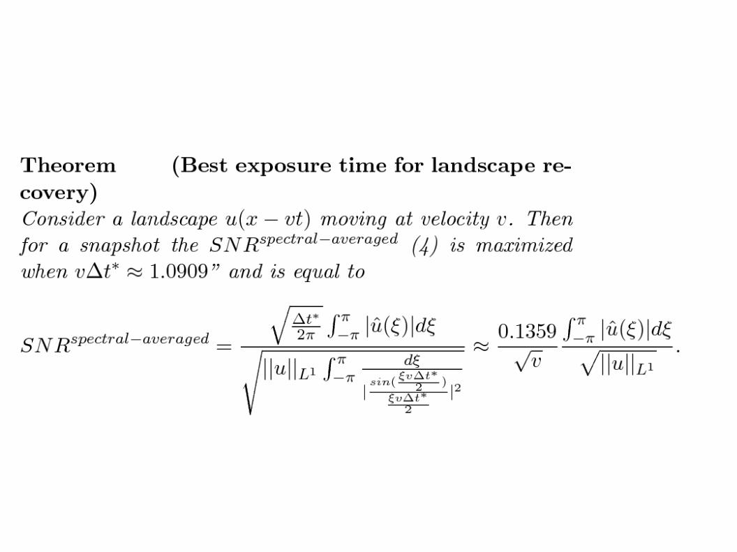
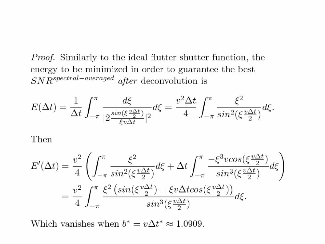
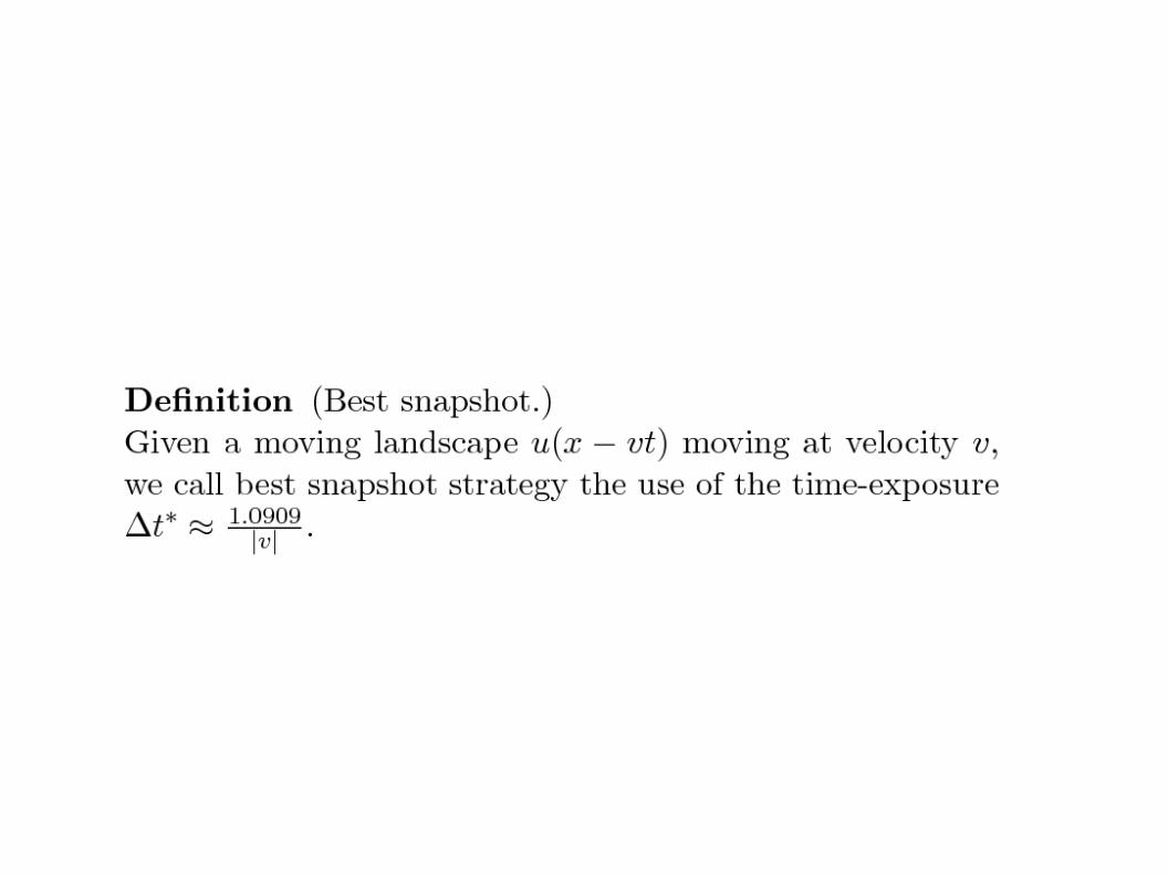
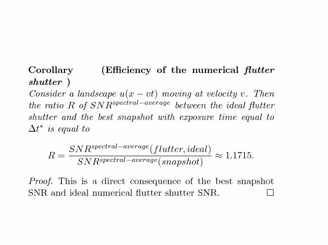
Theorem
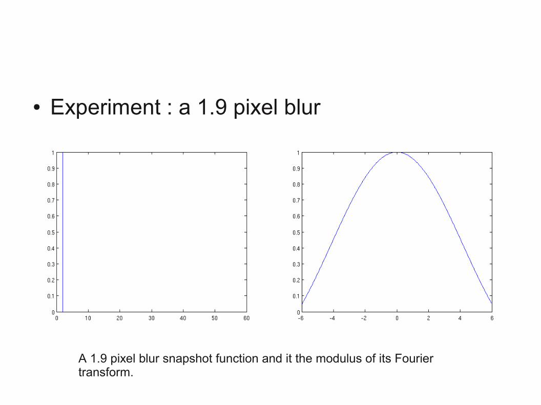
● Experiment : a 1.9 pixel blur
A 1.9 pixel blur snapshot function and it the modulus of its Fourier transform.
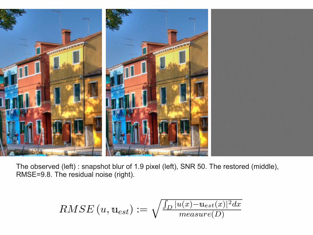
The observed (left) : snapshot blur of 1.9 pixel (left), SNR 50. The restored (middle), RMSE=9.8. The residual noise (right).

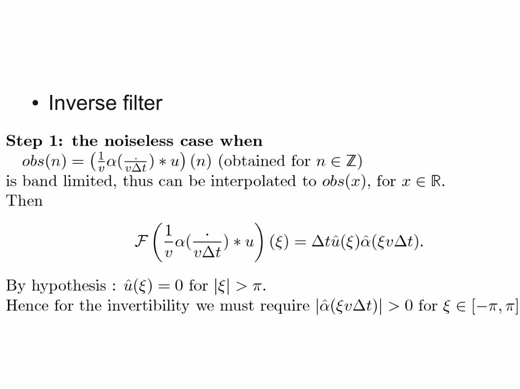
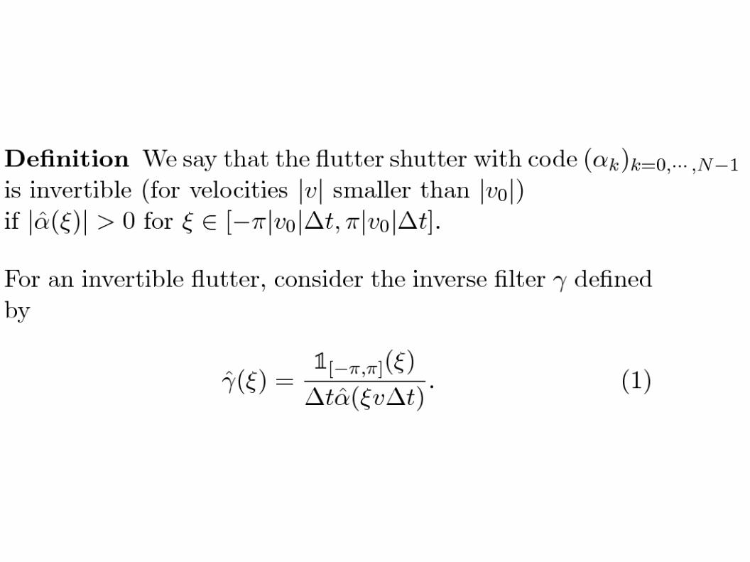
● Inverse filter
.
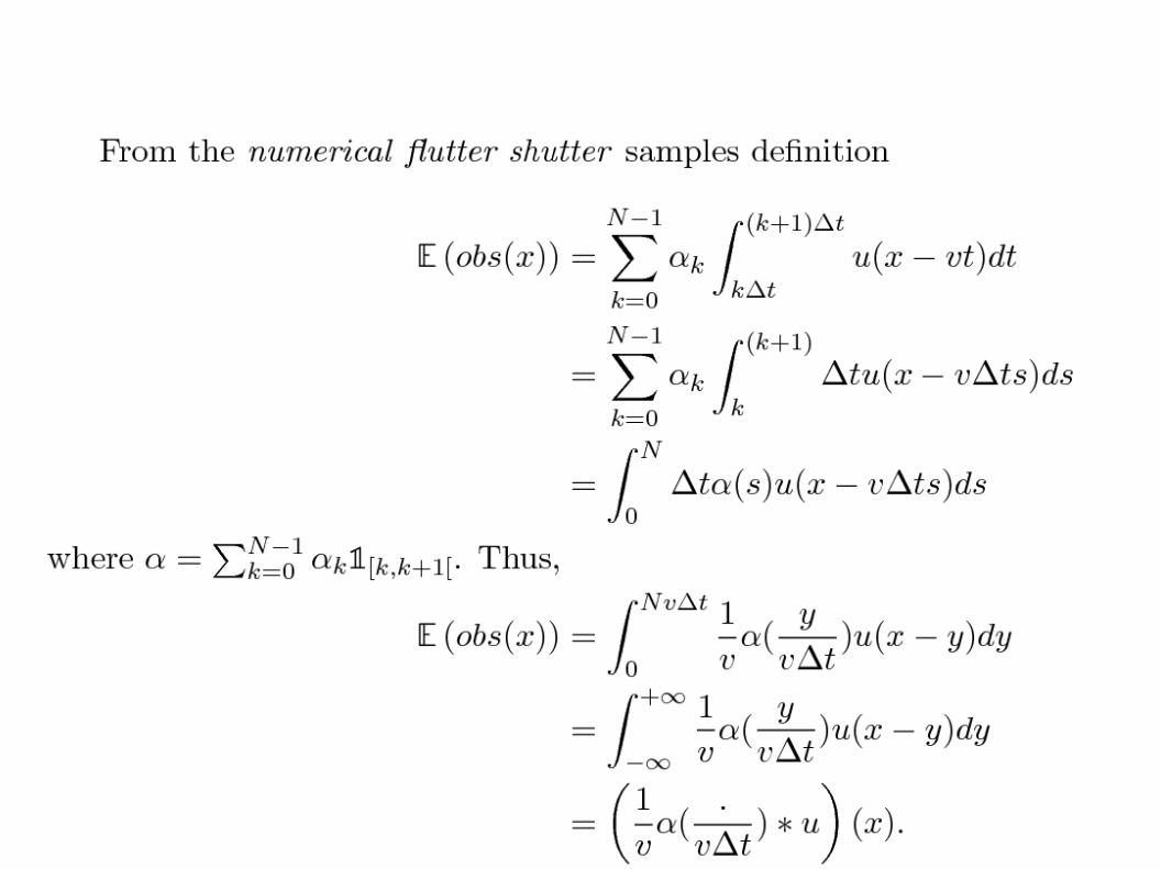
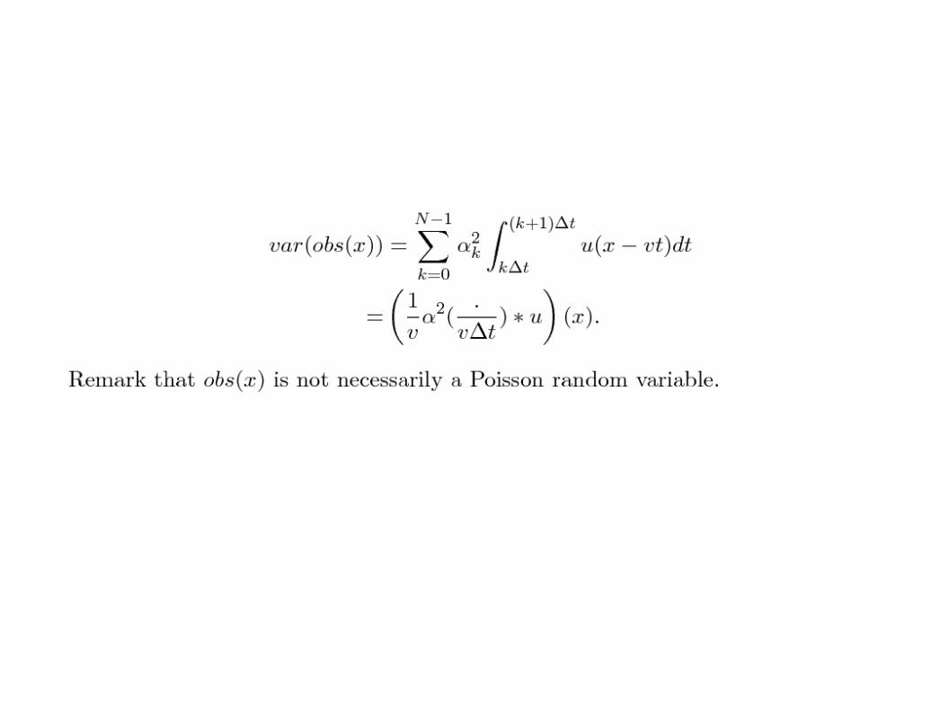
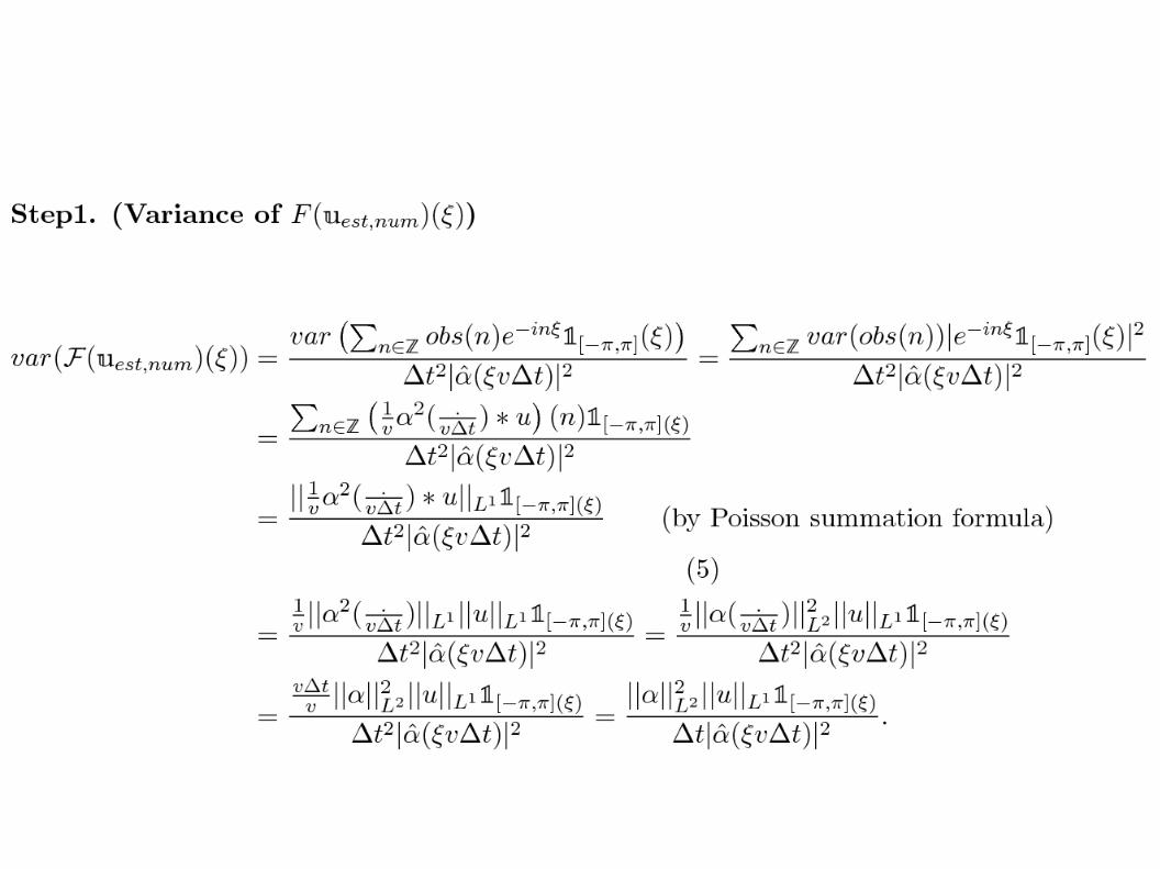
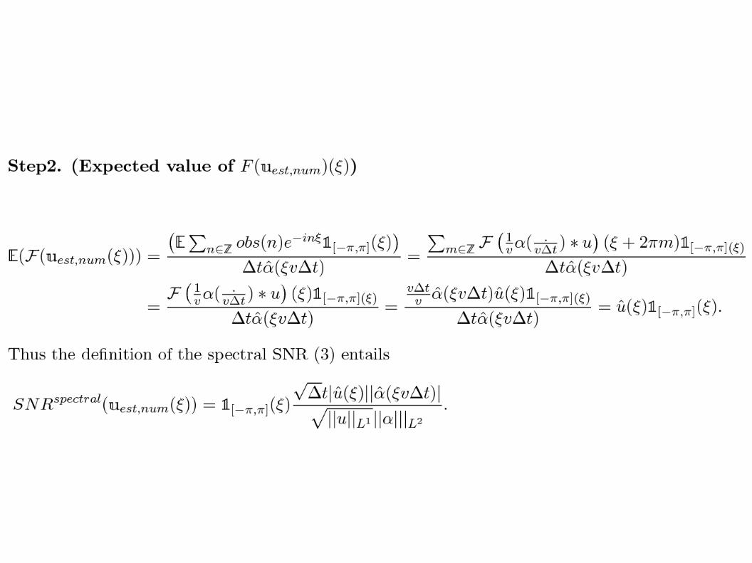
● Now we have a model for the observed
● We wish to compute the SNR
● And compare the SNR for different strategies (flutter shutter functions)
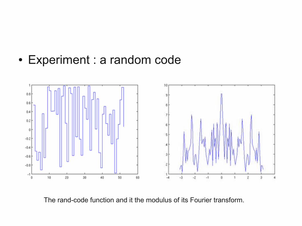
● Experiment : a random code
The rand-code function and it the modulus of its Fourier transform.
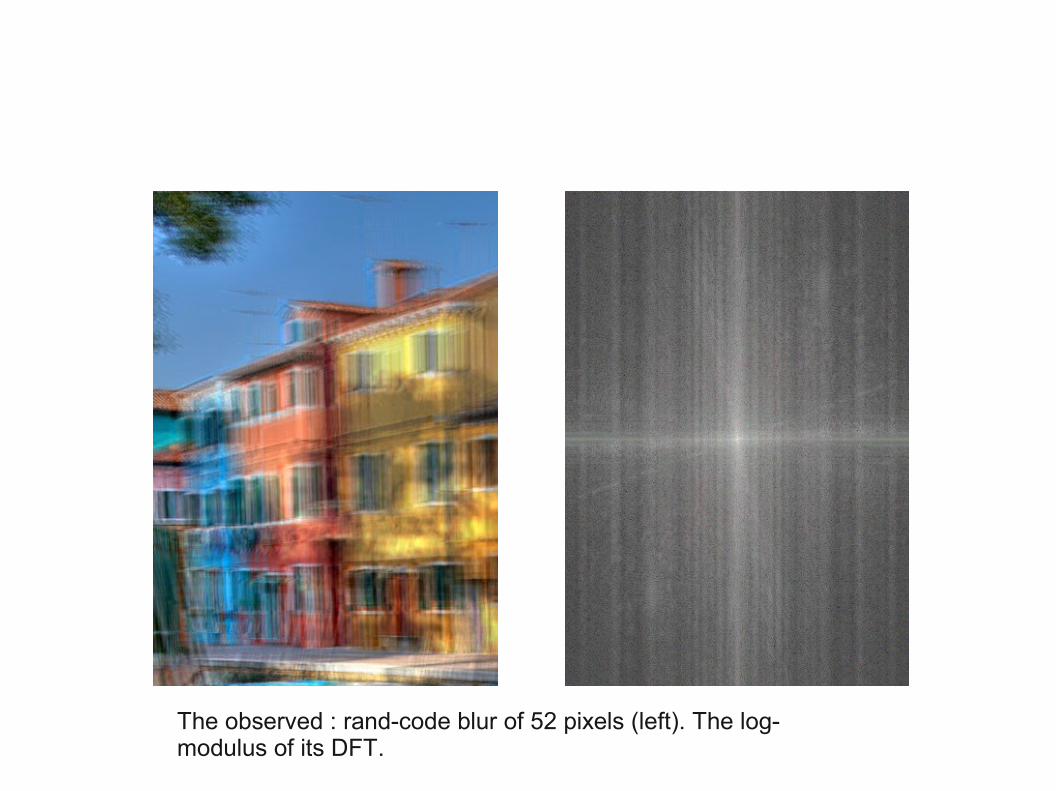
The observed : rand-code blur of 52 pixels (left). The log-modulus of its DFT.
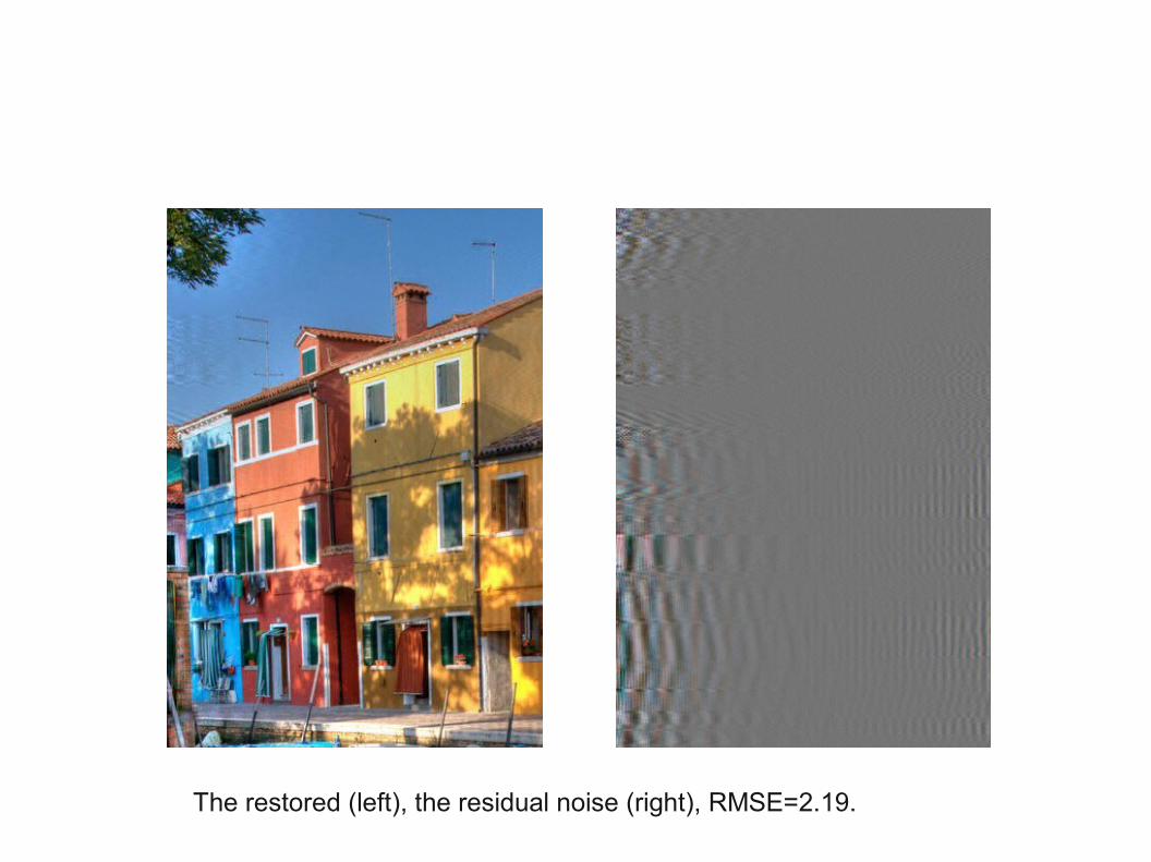
The restored (left), the residual noise (right), RMSE=2.19.
● White noise deconvolution (Raskar's code)


● White noise deconvolution (rand code)


● Numerical simulation, examples
The Flutter Shutter
● Numerical simulation

● Example 1 : the standard snapshot
The standard snapshot function and the modulus of its Fourier transform.
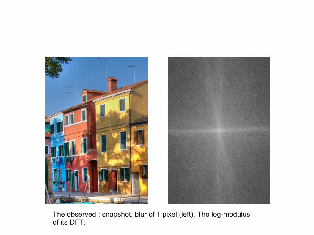
The observed : snapshot, blur of 1 pixel (left). The log-modulus of its DFT.
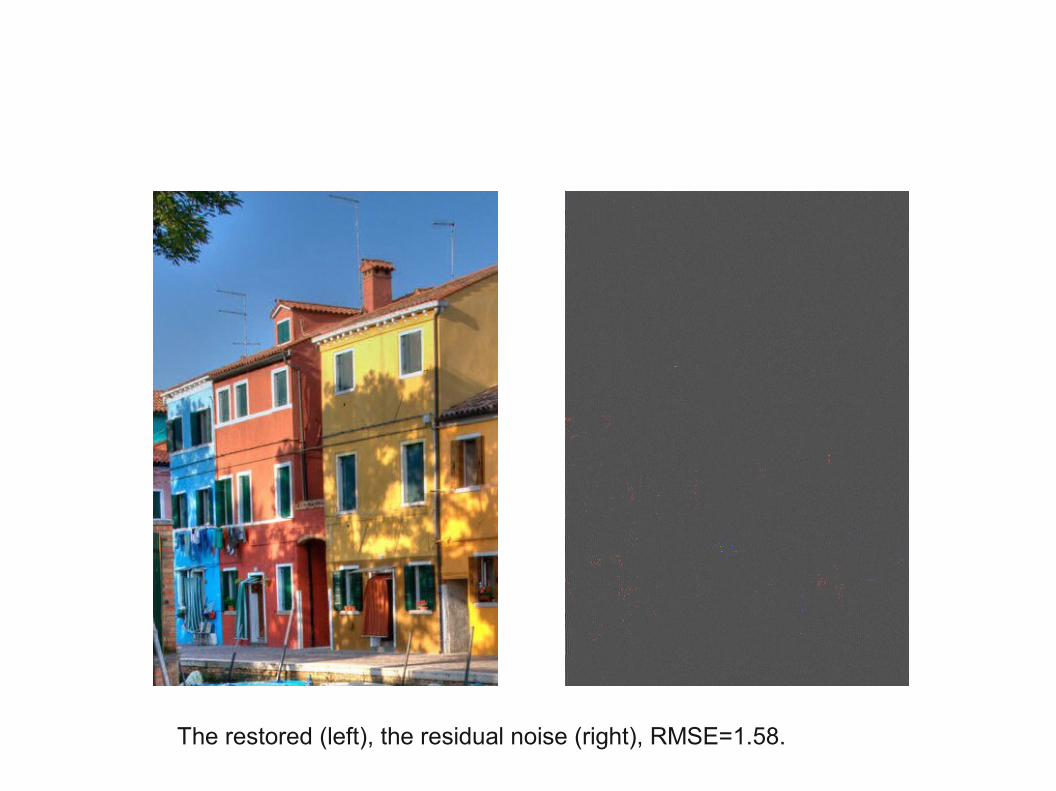
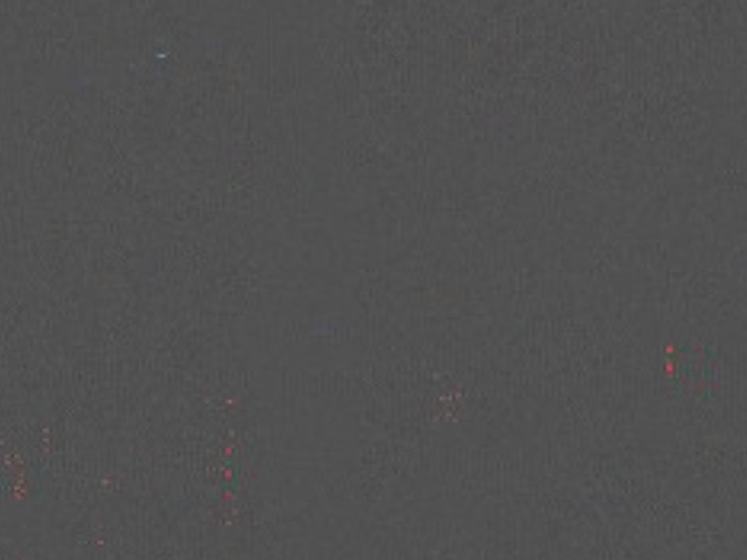
The restored (left), the residual noise (right), RMSE=1.58.
● Example 2 : Raskar's code
The Raskar function and the modulus of its Fourier transform.
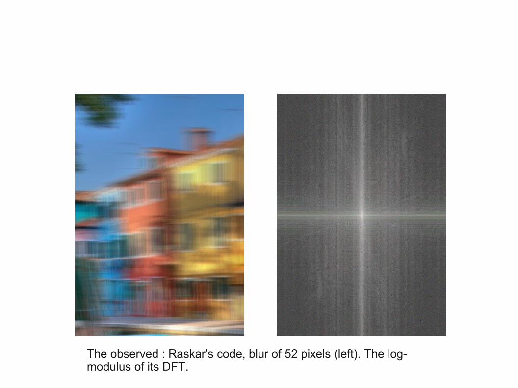
The observed : Raskar's code, blur of 52 pixels (left). The log-modulus of its DFT.
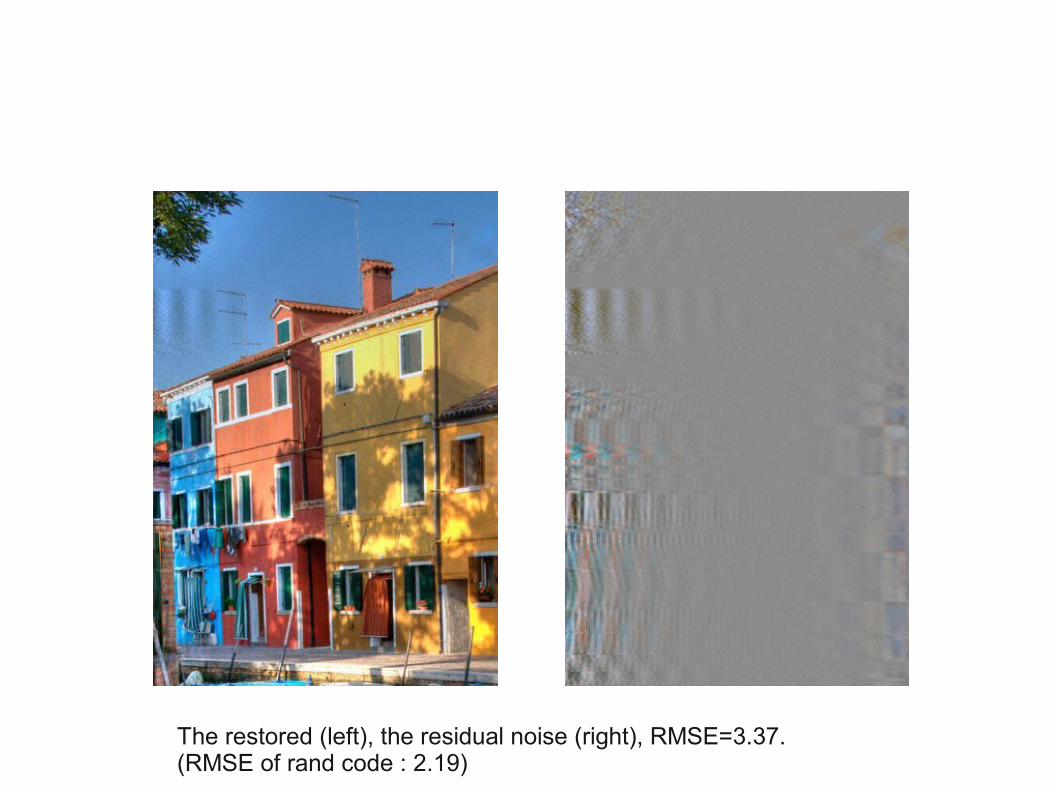
The restored (left), the residual noise (right), RMSE=3.37. (RMSE of rand code : 2.19)

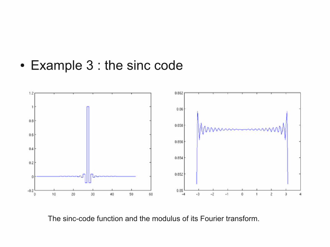
● Example 3 : the sinc code
The sinc-code function and the modulus of its Fourier transform.
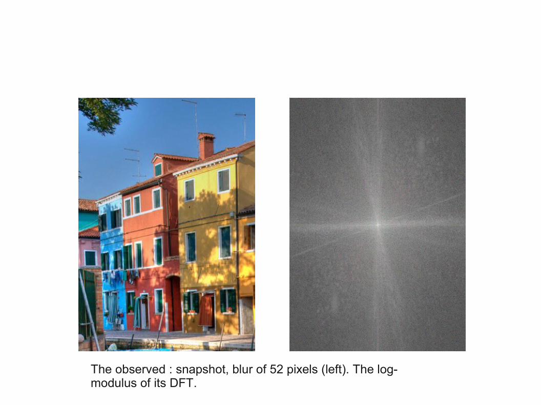
The observed : snapshot, blur of 52 pixels (left). The log-modulus of its DFT.
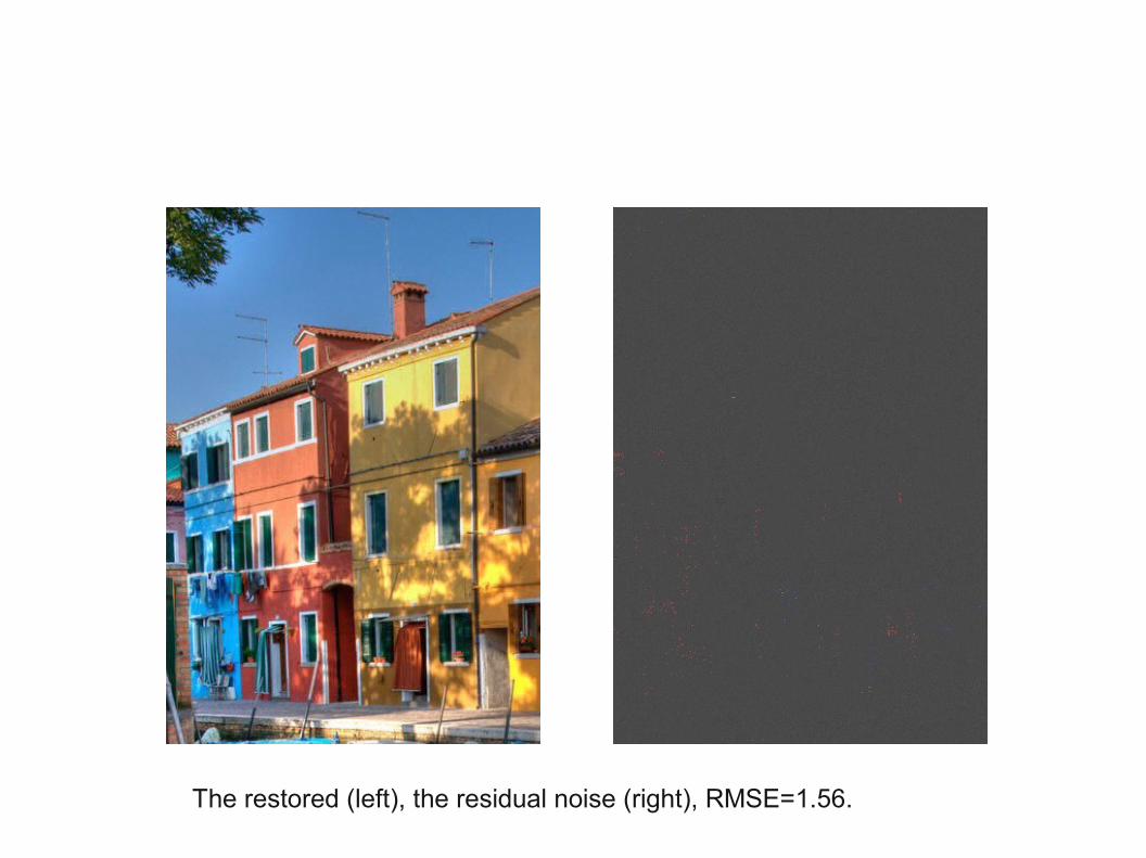
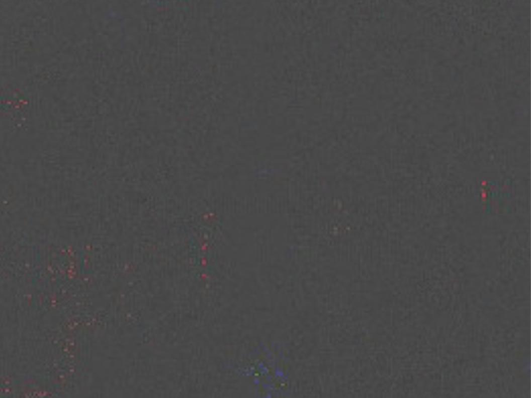
The restored (left), the residual noise (right), RMSE=1.56.
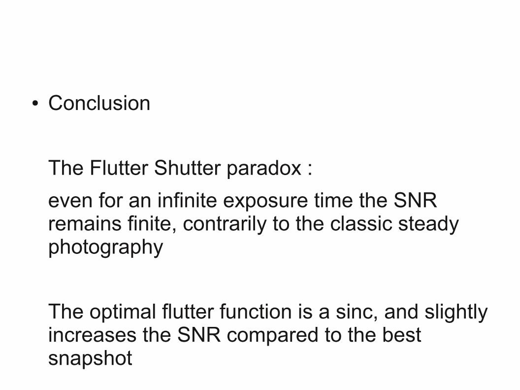
● Conclusion
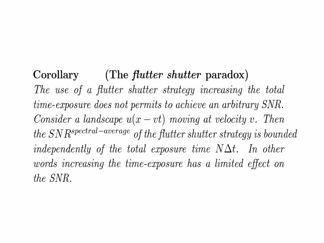
The Flutter Shutter paradox :
even for an infinite exposure time the SNR remains finite, contrarily to the classic steady photography
The optimal flutter function is a sinc, and slightly increases the SNR compared to the best snapshot
● Thanks!
● Try it : (IPOL)
https://edit.ipol.im/edit/algo/mrt_flutter_shutter/
Detailed description of the algorithm
Standard C++ code, commented
Running demo