The FThe Finite Element inite Element MethodMethod

FEM FOR BEAMS

A Practical CourseA Practical Course

CHAPTER 3:

CONTENTSCONTENTS INTRODUCTION FEM EQUATIONS

– Shape functions construction– Strain matrix– Element matrices – Remarks

EXAMPLE AND CASE STUDY– Remarks

INTRODUCTIONINTRODUCTION

The element developed is often known as a beam element.

A beam element is a straight bar of an arbitrary cross-section.

Beams are subjected to transverse forces and moments.

Deform only in the directions perpendicular to its axis of the beam.

INTRODUCTIONINTRODUCTION

In beam structures, the beams are joined together by welding (not by pins or hinges).

Uniform cross-section is assumed.FE matrices for beams with varying

cross-sectional area can also be developed without difficulty.

FEM EQUATIONSFEM EQUATIONS

Shape functions constructionStrain matrixElement matrices

Shape functions constructionShape functions construction

Consider a beam element

Natural coordinate system: a

x

d1 = v1

d2 = 1

d3 = v2

d4 = 2

x = - a = 1

x = a = 1

x,

2a

0

Shape functions constructionShape functions construction

33

2210)( vAssume that

In matrix form:

3

2

1

0

321)(

v or αp )()( Tv

)32(11 2

321

a

v

ax

v

x

v

Shape functions Shape functions constructionconstruction

1

11

(1) ( 1)

d(2)

d

v v

v

x

To obtain constant coefficients – four conditions

2

21

(3) (1)

d(4)

d

v v

v

x

At x= a or = 1

At x= a or = 1

d1 = v1

d2 = 1

d3 = v2

d4 = 2

x = - a = 1

x = a = 1

x,

2a

0

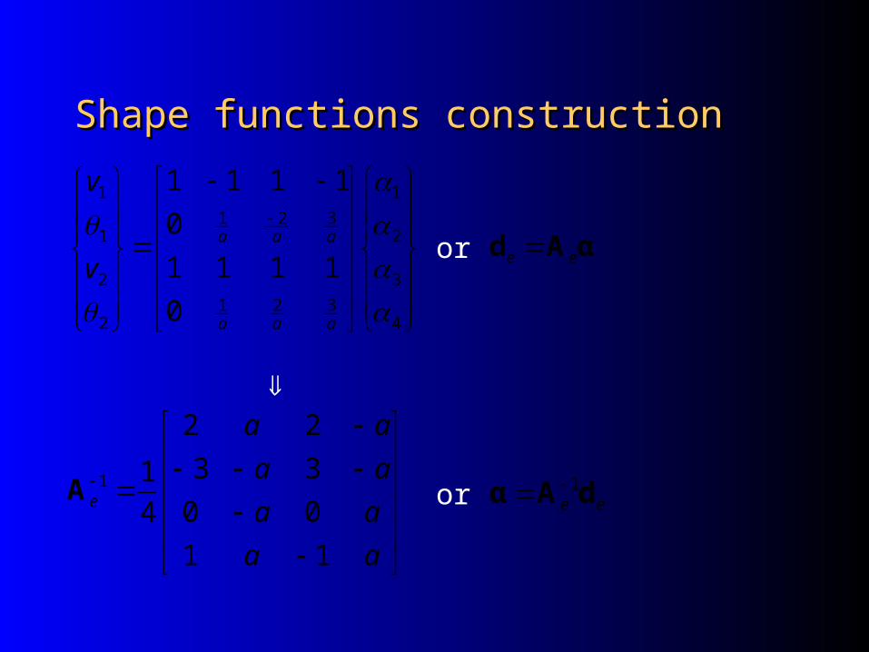
Shape functions constructionShape functions construction

4

3

2

1

321

321

2

2

1

1

0

1111

0

1111

aaa

aaa

v

v

or αAd ee

aa

aa

aa

aa

e

11

00

33

22

4

11A or ee dAα 1

Shape functions constructionShape functions construction

Therefore,

ev dN )(

where

)()()()()( 43211 NNNNe PAN

)1()(

)32()(

)1()(

)32()(

3244

341

3

3242

341

1

a

a

N

N

N

Nin which

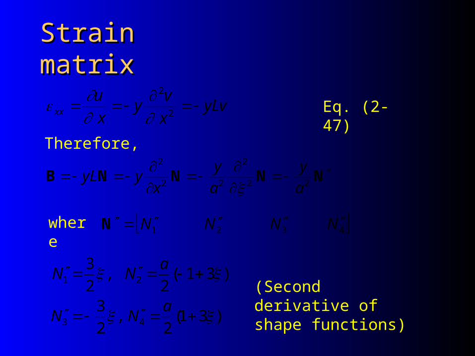
Strain matrixStrain matrix

yLvx

vy

x

uxx

2

2

Therefore,

NNNNB

22

2

22

2

a

y

a

y

xyyL

4321 NNNN Nwhere

)31(2

,2

3

)31(2

,2

3

43

21

aN N

a

N N(Second derivative of shape functions)

Eq. (2-47)

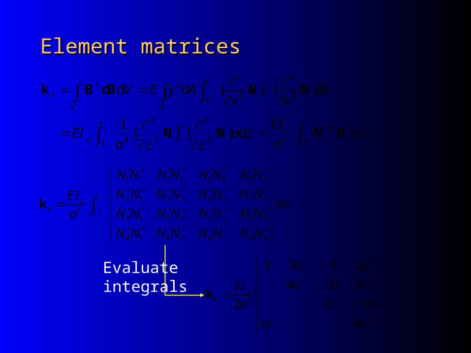
Element matricesElement matrices

dd][][1

d)()(dd

1

132

2

2

2

4

1

1

2

2

2

22

NNNN

NNBcBk

TzTz

Ta

aA

T

V

e

a

EIa

aEI

xxx

AyEV

1 1 1 2 1 3 1 4

1 2 1 2 2 2 3 2 4

3 13 1 3 2 3 3 3 4

4 1 4 2 4 3 4 4

dze

N N N N N N N N

N N N N N N N NEI

N N N N N N N Na

N N N N N N N N

k

2

22

3

4.

33

234

3333

2

asy

a

aaa

aa

a

EI zek

Evaluate integrals

Element Element matricesmatrices

1

1

1 1 1 2 1 3 1 4

1 2 1 2 2 2 3 2 4

13 1 3 2 3 3 3 4

4 1 4 2 4 3 4 4

d d d d

d

aT T Te a

V A

V A x A a

N N N N N N N N

N N N N N N N NAa

N N N N N N N N

N N N N N N N N

m N N N N N N

2

22

8.

2278

6138

13272278

105

asy

a

aaa

aa

Aae

m

Evaluate integrals

Element matricesElement matrices

2

2

111

1 112 3

1223

2423

d d dy

f

y

y ss

f a

ssT Te b s f y

y ssV S

f as

s

f a ffN

mmNf V f S f a

f a ffN

mN m

f N N

eeeee fdmdk

RemarksRemarks

Theoretically, coordinate transformation can also be used to transform the beam element matrices from the local coordinate system to the global coordinate system.

The transformation is necessary only if there is more than one beam element in the beam structure, and of which there are at least two beam elements of different orientations.

A beam structure with at least two beam elements of different orientations is termed a frame or framework.

EXAMPLEEXAMPLEConsider the cantilever beam as shown in the figure. The beam is fixed at one end and it has a uniform cross-sectional area as shown. The beam undergoes static deflection by a downward load of P=1000N applied at the free end. The dimensions and properties of the beam are shown in the figure.

P=1000 N

0.5 m

0.06 m

0.1 m

E=69 GPa =0.33

EXAMPLEXAMPLEE

Step 1: Element matrices

33 6 41 10.1 0.06 1.8 10 m

12 12zI bh

9 6

3

6 -2

3 0.75 3 0.7569 10 1.8 10 0.75 0.25 0.75 0.125

3 0.75 3 0.752 0.25

0.75 0.125 0.75 0.25

3 0.75 3 0.75

0.75 0.25 0.75 0.1253.974 10 Nm

3 0.75 3 0.75

0.75 0.125 0.75 0.25

e

K k

Exact solution:4

40y y

vEI f

x

2

( ) (3 )6 y

Pxv x L x

EI

0yf

P=1000 N

0.5 m

E=69 GPa =0.33

3

( )3 y

PLv x L

EI

= -3.355E10-4 m

Eq. (2.59)

EXAMPLEXAMPLEE

Step 1 (Cont’d):

1 1

1 16

2 2

2 2

?3 0.75 3 0.75 unknown reaction shear force

?0.75 0.25 0.75 0.125 unknow3.974 10

3 0.75 3 0.75

00.75 0.125 0.75 0.25

v Q

M

v Q P

M

DK F

n reaction moment

Step 2: Boundary conditions1 1 0v

1 1

1 16

2 2

2 2

03 0.75 3 0.75

00.75 0.25 0.75 0.1253.974 10

3 0.75 3 0.75

00.75 0.125 0.75 0.25

v Q

M

v Q P

M

P=1000 N

0.5 m

E=69 GPa =0.33

1 1 0v

EXAMPLEXAMPLEE Step 2 (Cont’d):

6 -23 0.753.974 10 Nm

0.75 0.25

K

Therefore, K d = F, where

dT = [ v2 2] , 1000

0

F

Step 3: Solving FE equation(Two simultaneous equations) v2 = -3.355 x 10-4 m

2 = -1.007 x 10-3 rad

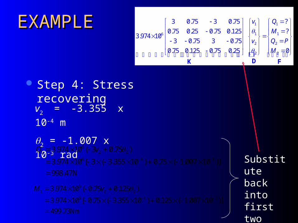
EXAMPLEXAMPLEE

Step 4: Stress recovering

v2 = -3.355 x 10-4 m

2 = -1.007 x 10-3 rad

61 2 2

6 4 3

3.974 10 ( 3 0.75 )

3.974 10 [ 3 ( 3.355 10 ) 0.75 ( 1.007 10 )]

998.47N

Q v

61 2 2

6 4 3

3.974 10 ( 0.75 0.125 )

3.974 10 [ 0.75 ( 3.355 10 ) 0.125 ( 1.007 10 )]

499.73Nm

M v

Substitute back into first two equations

1 1

1 16

2 2

2 2

?3 0.75 3 0.75

?0.75 0.25 0.75 0.1253.974 10

3 0.75 3 0.75

00.75 0.125 0.75 0.25

v Q

M

v Q P

M

DK F

RemarksRemarks

FE solution is the same as analytical solution Analytical solution to beam is third order

polynomial (same as shape functions used) Reproduction property

CASE STUDYCASE STUDY

Resonant frequencies of micro resonant transducer

Membrane

Bridge

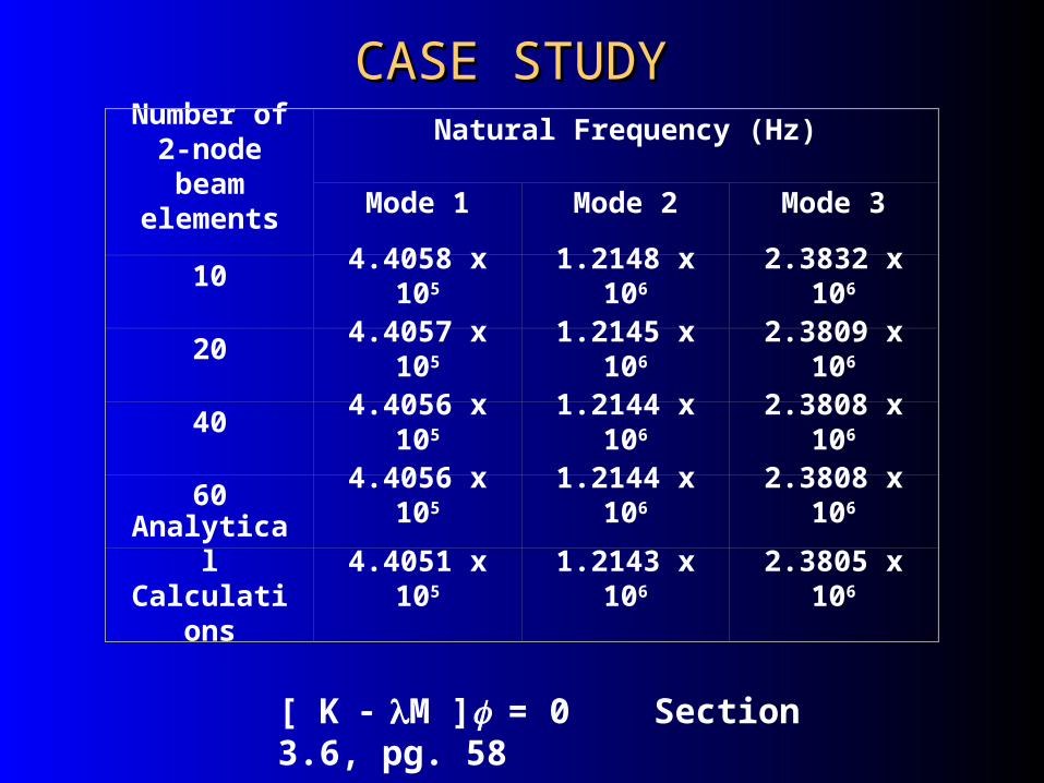
CASE CASE STUDYSTUDY

Number of 2-node beam elements

Natural Frequency (Hz)

Mode 1 Mode 2 Mode 3

10 4.4058 x 105 1.2148 x 106 2.3832 x 106

20 4.4057 x 105 1.2145 x 106 2.3809 x 106

40 4.4056 x 105 1.2144 x 106 2.3808 x 106

60 4.4056 x 105 1.2144 x 106 2.3808 x 106

Analytical Calculations

4.4051 x 105 1.2143 x 106 2.3805 x 106

[ K M ]= 0 Section 3.6, pg. 58

CASE STUDYCASE STUDY

Mode 1 (0.44 MHz)

0

0.2

0.4

0.6

0.8

1

1.2

0 20 40 60 80 100

x (um)

Dy

(um

)

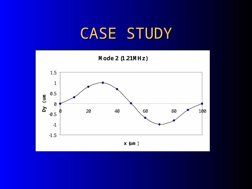
CASE STUDYCASE STUDYMode 2 (1.21MHz)

-1.5

-1

-0.5

0

0.5

1

1.5

0 20 40 60 80 100

x (um)

Dy

(um

)

CASE STUDYCASE STUDY

Mode 3 (2.38 MHz)

-1.5

-1

-0.5

0

0.5

1

1.5

0 20 40 60 80 100

x (um)

Dy

(um

)