The Financial Modeling of

Property/Casualty Insurance Companies by Douglas M. Hodes Tony Neghaiwi, FCAS

J. David Cummins Richard Phillips

Sholom Feldblum, FCAS, ASA

THE FINANCIAL MODELING OF PROPERTY-CASUALTY INSURANCE COMPANIES

Douglas M. Hodes, Tony Neghaiwi,

J. David Cummins, Richard Phillips, and

Sholom Feldblum

Abstract

This paper describes a financial model currently being used by a major U.S. multi-line insurer. The model, which was first developed for solvency monitoring purposes, is now being employed for a variety of internal management purposes, including (i) the allocation of equity to corporate units, thereby allowing measurements of profitability by business segment and by policy year, as well as analysis of the progression of “free surplus,” (ii) the analysis of major risks, such as inflation risks, interest rate risks, and reserving risks, that have heretofore been difficult to quantify, and (iii) consideration of varying scenarios on the company’s financial performance, both of macroeconomic conditions as well as of the insurance environment.

This paper begins with the genesis of the model and with its structure. It moves on to equity considerations and to performance measurement. It then discusses the major risks that have heretofore resisted actuarial analysis, such as interest rate risk (inflation risk), reserving risk, and scenario testing. The paper shows how cash flow financial models can deal with global risks that simultaneously affect various aspects of the insurer’s operations, delineating the resulting changes in the company’s performance.

The Financial Modeling of Property-Casualty Insurance Companies

(Authors)

DouglasM. Hades is a Vice President and Corporate Actuary with the Liberty Mutual Insurance Company in Boston, Massachusetts. He oversees the Corporate Actuarial and Corporate Research divisions of the company, and he is responsible for capital allocation, financial modeling, surplus adequacy monitoring, and reserving oversight functions.

Mr. Hodes is a graduate of Yale University (1970) and he completed the Advanced Management Program at Harvard University in 1988. He is a Fellow of the Society of Actuaries, a member of the American Academy of Actuaries, a member of the American Academy of Actuaries Life Insurance Risk-Based Capital Task Force, and a former member of the Actuarial Committee of the New York Guaranty Association. Before joining Liberty Mutual, Mr. Hodes was a Vice President in Corporate Actuarial at the Metropolitan Life Insurance Company, where his responsibilities included the development of a life insurance financial model.

Mr. Hodes is the author of “Interest Rate Risk and Capital Requirements for Property-Casualty Insurance Companies” (with Mr. Sholom Feldblum) and of ‘Workers’ Compensation Reserve Uncertainty” (with Dr. Gary Blumsohn and Mr. Feldblum). These papers apply actuarial and financial techniques to quantify risks associated with interest rate movements and with unexpected reserve developments. In addition, Mr. Hodes is a frequent speaker at actuarial conventions on such topics as dynamic financial analysis and risk-based capital.

Tony Neghaiwi, FCAS, is an Associate Actuary with the Liberty Mutual Insurance Company, where he is responsible for the development and the maintenance of the model described in this paper.

Dr. J. David Cummins is the Harry J. Loman Professor of Insurance and Risk Management and Executive Director of the S. S. Huebner Foundation for Insurance Education at the Wharton School of the University of Pennsylvania. Dr. Cummins’ primary research interests are the financial management of insurance companies, the economics of insurance markets, and insurance rate of return and solvency regulation. He is the editor of the Journal of Risk and insurance and past president of the American Risk and fnsurance Association and the Risk Theory Society.

Dr. Cummins has written or edited fourteen books and published more than forty journal articles in publications such as the Journal of Finance, Management Science, the Journal of Banking and Finance, the Journal of Economic Perspectives, the Journal of Risk and Uncertainty, and the Astin Bulletin. Among his recent publications are “Insolvency Experience, Risk-Based Capital, and Prompt Corrective Action in Property-Liability Insurance,” Journal of t3anking and Finance (1995); “Pricing Insurance Catastrophe Futures and Call Spreads: An Arbitrage Approach,” Journal of fixed income (1995); and ‘Capital Structure and the Cost of

Equity Capital in Property-Liability Insurance,” Insurance: Mathematics and Economics (1994). His paper, “An Asian Option Approach to Pricing Insurance Futures Contracts,” was awarded the Best Paper prize at the 1995 AFIR Colloquium in Brussels, Belgium.

Dr. Cummins has served as consultant to numerous business and governmental organizations. He has consulted and testified on the cost of capital in insurance for organizations such as the National Council on Compensation Insurance and Liberty Mutual Insurance Group. He has conducted research on insurance cycles and crises for the National Association of Insurance Commissioners, and he has testified for several state departments of insurance and the U.S. Department of Justice. He advised the Alliance of American Insurers on risk-based capital in property-liability insurance.

Dr. Richard 0. Phillips is an Assistant Professor of Risk Management and Insurance at Georgia State University. He received his Ph.D. in Finance and Insurance in 1994 from the Wharton School, University of Pennsylvania.

Dr. Phillips’s recent publications on topics related to insurance company financial modeling include “Financial Pricing of Insurance in the Multiple-Line Insurance Company” (with J. David Cummins) and “The Economics of Risk and Insurance.” From March 1992 through January 1994, Dr. Phillips was a principle investigator in the Alliance of American Insurers project to develop a risk-based capital cash flow solvency model, which used an earlier version of the model described in this paper.

Dr. Phillips is a frequent speaker at research seminars on such topics as cash flow modeling, financial pricing, and insurance regulation.

Shalom Feldblum is an Assistant Vice President and Associate Actuary with the Liberty Mutual Insurance Company. He holds the FCAS, CPCU, ASA, and MAAA designations, and he is a member of the CAS Syllabus Committee and of the American Academy of Actuaries Task Force on Risk- Based Capital. He is the author of numerous papers on ratemaking, loss reserving, statutory accounting, insurance economics, competitive strategy, investment theory, solvency monitoring, and finance, which have appeared in Best’s Review, the CPCU Journal, the Proceedings of the Casualty Actuarial Society, the Acfuarial Digest, the CAS Forum, the Journal of insurance Regulation, the Journal of Reinsurance and the CAS Discussion Paper Program. He was the recipient of the CAS Michelbacher Prize in 1993 for his paper on “Professional Ethics and the Actuary.”

In addition to the two papers co-authored with Douglas Hodes (see above), Mr. Feldblum is the author of “European Approaches to Insurance Solvency,” which describes the British and Finnish foundations upon which the model described in this paper is based, and “Forecasting the Future: Stochastic Simulation and Scenario Testing,” which describes the use of scenario testing in financial models.

6

THE FINANCIAL MODELING OF PROPERTY-CASUALTY INSURANCE COMPANIES

Introduction

The existing literature on the financial modeling of property-casualty insurance companies consists predominantly of theoretical discourses seen through the eyes of the research actuary. The sophistication of complex stochastic simulation is extolled; the practical implementation of the models is rarely considered.

This paper, in contrast, describes a financial model currently being used by a major U.S. multi-line insurer. The first version of the model was developed in 1993 for solvency monitoring purposes. In the three years since then, the model has been greatly expanded and it has been applied to a variety of internal management uses, including (i) the allocation of equity to corporate units, thereby allowing measurements of profitability by business segment and by policy year, as well as analysis of the progression of “free surplus,” (ii) the analysis of major risks, such as inflation risks, interest rate risks, and reserving risks, that have heretofore been difficult to quantify, and (iii) consideration of varying scenarios on the company’s financial performance, both of macroeconomic conditions as welt as of the insurance environment.

Many multiline insurance enterprises are complex organizations, with dozens of distinct yet interrelated parts. This complexity is the major stimulus for financial models that consider the workings of the entire corporation. At times, however, this complexity renders cumbersome the documentation of the models. To facilitate the readability of this paper, the numerical exhibits are contained in the appendices, so that the text flows more easily.

This paper discusses the following topics:

rc Genesis: that is, the factors that stimulated the development of the model. z Structure: that is, the types of underwriting and financial operations and the types of

time periods with which it deals. Since this paper is not just a theoretical discourse but also a practical description of a working model, it shows the actual inputs and outputs: what variables must be provided by the user, and several types of tables, charts, and graphs that are produced by the model.

c Equity considerations: how net worth (“economic surplus”) is determined by line of business (LOB) and how the progression of “free surplus” is viewed.

* Profitability measures: given the actual (past) or expected (future) cash flows, along with the progression of LOB surplus and of free surplus, how profitability is measured.

The financial model described here is particularly important for evaluating three types of risk that are not easily analyzed by other methods:

* Risks that simultaneously affect several components of an insurance company’s operations, such as inflation risks and interest rate risks.

* Risks that results from an overall change in the external economic environment, such as recessions, or from changes in the insurance industry as a whole, such as underwriting cycle movements.

* Risks that depend on complex, random fluctuations, such as reserving risks.

This paper shows how the financial model deals with these types of risk

Genesis of the Model

The company’s modeling efforts were stimulated by several developments:

0 From 1990 through 1993, the NAIC developed new risk-based capital requirements for both property-casualty and life insurance companies. Many observers have criticized the NAIC efforts from three perspectives:

A The risk-based capital formulas are based on accounting figures. B. Some of the RBC charges seem to be “ad hoc” factors lacking actuarial or financial

justification. C. Several important risks are not even considered.

For example, these critics have said that

A The statutory financial statements that underlie the risk-based capital formulas should be replaced by cash flow approaches or by market value accounting, both for solvency monitoring by state regulators and for management evaluation of the company’s performance.1

B. The reserving risk charges in the NAIC formula, which are based on the NAIC “worst case year” method coupled with a large dose of “regulatory judgment,” should be replaced by rigorous actuarial analyses of reserve variability. Similar analyses should be undertaken for the underwriting risk of new business (“written premium risk” in RBC terminology) and for the risks of reinsurance collectibility.

C. Interest rate risk, which affects both assets and liabilities, should be incorporated into the formula. Interest rate risk is particularly difficult to model in the NAIC formula, since (i) it is a market value phenomenon, not an accounting phenomenon, and (ii) it is intertwined with other risks, such as inflation risks and reserving risks.

@ Meanwhile, the American Academy of Actuaries has proposed an expanded vision of the Appointed Actuary’s role, covering not just opinions on the reasonableness of loss and loss adjustment expense reserves but also statements on the financial strength of the insurance enterprise under varying longer term scenarios and on the resilience of the company to different types of adverse external conditions. The model described in this paper is the practical implementation of the AAA vision: it shows the cash flows of the company under varying future scenarios.

t Compare especially Robert P. Sutsic, “Solvency Measurement for Property-Liability Risk-Based Capital Applications,” Journal of Risk and Insurance, Volume 61, Number 4 (December 1994), pages 656-690, who discusses the “measurement bias” introduced when GAAP or statutory accounting statements are used for solvency monitoring purposes.

8

8) Soon after this model was implemented, the authors changed their emphasis from solvency monitoring to profitability measurement. When insurance companies fare poorly, financial models are important for monitoring solvency. In the early 1990’s, the multi-line insurer using this model fared extremely well, because of both strong industry profits in its major lines of business and its own favorable performance relative to its peer companies. It elected to expand into new markets, develop new products, and acquire other (related) businesses. It required a sophisticated management model, in order to judge both the immediate risks and the long-term uncertainties associated with the new projects, as well as the capital needed to safely undertake them.

Description of the Model

The financial model described here provides three types of results:

0 The model itself uses a cash-flow approach, following the method developed by the British Solvency Working Party in the 1980’s? The cash flow results are particularly important for Appointed Actuary work and for comparing the effects of different scenarios.

B For management purposes, the model can generate statutory accounting results, as would be needed for pro-forma financial statements. Statutory accounting is an important constraint on insurance company strategy. These results are useful for analyzing the progression of “free surplus”3

b By selecting appropriate discount rates for loss outflows and for investment inflows, the analyst can determine market values of the insurance enterprise at various points in time

2 For a more complete presentation of the British Solvency Working Party approach, see Chris D. Daykin, G. D. Bernstein, S. M. Coutts. E. R. F. Devitt. G. B. Hey, D. I. W. Reynolds, and P. 0. Smith, “Assessing the Solvency and Financial Strength of a General insurance Company,” Journal of the institute of Actuaries, Volume 114, Part 2 (1987), pages 227-310; Chris D. Daykin, G. D. Bernstein, S. M. Coutts, E. Ft. F. Devitt, G. B. Hey, D. I, W. Reynolds, and P. D. Smith, “The Solvency of a General Insurance Company in Terms of Emerging Costs,” in J. David Cummins and Richard Derrig, Financial Mode/s of hsurance Solvency (Boston: Kluwer Academic Publishers, 1989), pages 87-149, or in AST/N Bulletin, Volume 117, No. 1 (1987), pages 85-132; Chris D. Daykin and G. B. Hey, “Managing Uncertainty in a General Insurance Company,” Journal of the hsfitute of Acfuaries, Volume 117, Part 2, No. 467 (September 1990), pages 173-259. The recent text by Chris D. Daykin, Teivo Pentiktiinen, and M. Pesonen, Practical Risk Theory for Actuariss (Chapman and Hall, 1994), combines the cash flow approach of the British Solvency Working Party and the accounting approach of the Finnish Working Party. In addition, that textbook emphasizes stochastic procedures to develop scenarios, whereas the model described here uses stochastic procedures for risks that are random and “scenario building” for global risks with interdependent elements.

3 For reasons of space, the translation of net cash flows and market values into statutory values is not shown in the exhibits in this paper. The required work is primarily accounting, not actuarial, and it is not germane to the theoretical framework of the model.

9

or under various scenarios. These results are important for determining profitability of existing and of new business.

Past and Future Business

For past business, the model uses actual company results, along with

. chain ladder paid loss development for the run-off of existing reserves,

. stated coupon rates for fixed income securities, and

. expected dividend yields on common stocks for investment returns.

Two further adjustments are made:

0 The company has large investments in mortgage-backed securities, with high prepayments as borrowers change homes or simply refinance their mortgages when interest rates are low. The expected cash flows are adjusted in each scenario for these options, and the effects are shown in the exhibits. Similar adjustments are used for other options, such as call provisions in corporate bonds.4

@ About half of the company’s workers’ compensation business is written on loss sensitive contracts. The premium payment patterns extend for about ten years after the policy expires, as shown in the exhibits.

For future years’ operations, the cash flows are based on a combination of company business plans and actuarial projections. For instance, written premium by line of business is taken from the business plans. The anticipated loss and LAE ratios and the anticipated underwriting expense ratios are actuarial projections. These figures are combined with the payment and collection patterns developed from past business to model the cash flows from new business.

Base Case and Alternative Scenarios

To illustrate the power of the financial model, two scenarios are shown in the exhibits and discussed in the text.

0 The base case scenario assumes an annual inflation rate of 4.0% and growth in real exposures of 2.0%, for a nominal growth in underwriting cash flows of 6.1% per annum. These assumptions affect premiums, losses, and expenses for each line of business. In practice, of course, the assumed growth in real exposures will vary by line, depending on the company’s business plans. [The model allows for separate assumptions by line and by policy year, which are used in actual work.]

The average pre-tax yield on the bond portfolio held by the company is 8.3% per annum. The assumed stock dividend yield is 2.75% per annum, and the rate of growth in stock values is 8.0% per annum, providing an annual return on common stocks of 10.75%.

4 These expected cash inflows are similar to those required in the new NAIC risk-based capital “supplementary asset schedule” used to measure interest rate risk; see Douglas M. Hodes and Sholom Feldblum, “Interest Rate Risk and Capital Requirements for Property- Casualty Insurance Companies” (CAS Part 10 examination study note).

10

The federal income tax rate is 35%. Since income taxes are explicitly included in the cash flows, the model uses an after tax discount rate of 5.4% to determine the present values of insurance operations (when present values are used in the analyses). [5.4% is 8.3% * (l-35%).] The expected after-tax yield on the company’s investment portfolio is about 5.7%, reflecting the higher returns on the common stocks.

@ The alternative scenario assumes that the inflation rate increases by 200 basis points to 6.0% with a concomitant increase in the pre-tax bond yield on new investments to 10.3%. [The market value of existing fixed-income securities, of course, falls when the interest rate rises, with the magnitude of the effect depending on the duration of the fixed income portfolio.] The growth in real exposures remains 2.0%, for a nominal growth in underwriting cash flows of 8.1%. The immediate effect on underwriting and investment results is twofold:

A. For each line of business, the new rates affect premiums, losses, and expenses. When rates first increase, however, the nominal losses grow more quickly than premiums, leading to an initial increase in the loss ratios.

B. Market values of bonds and of mortgages, as well as of mortgage-backed securities, tall when interest rates rise. Initially, common stock prices also drop when interest rates increase, as noted by many investment economists. 5 This decline, however, is fully recovered in the subsequent two years, since the simultaneous rise in inflation and interest rates causes no change in the real equity value of corporations.

The federal income tax rate remains 35%. The after tax discount rate for insurance cash flows now changes to 6.7%.

The summary assumptions for the base case scenario and for the alternative scenario are shown on Exhibit 1 of Appendix A. Exhibits 2 through 5 of Appendix A show the projected written premium, incurred loss plus loss adjustment expense, and other underwriting expenses, as well as the loss ratios, expense ratios, and combined ratios, for new business, under each of the two scenarios.

The exhibits shows ten years of new business, as would be used in a “going-concern” valuation. For clarity of exposition, the text discusses a single year of new business (policy year 1995), though we show exhibits and graphs for ten years of new writings as well. For the “progression of free surplus,” the exhibits also show the anticipated 1996 written premiums.

6 See, for example, Eugene F. Fama and G. William Schwert, “Asset Returns and Inflation,” Journal of Financial Economics, Volume 5 (1977), pages 115-146. Fama and Schwert’s paper uses data which is now 20 years “out-of-date.” Other analysts have replicated the Fama and Schwert results, though the theoretical explanations vary from author to author; see, for instance, Martin Feldstein, I’ Inflation and the Stock Market,” American Economic Review, Volume 70 (December 1980), pages 839-487. To parameterize our model, we replicated the Fama and Schwert study using the most recent 20 years of data from the lbbotson and Sinquefield indices. The signs of the coefficients in our analysis were generally consistent with the signs found by Fama and Schwert, though the magnitudes of the coefficients were dampened.

11

Asset Returns

The financial model uses the expected cash flows from each group of securities, not the stated cash flows. The difference is particularly great for mortgages and for mortgage backed securities (which form significant proportions of life insurance and property-casualty insurance investment portfolios, respectively), for two reasons:

0 As borrowers move to different homes, they pre-pay the mortgages. This effect occurs even if interest rates do not change. It is dependent on interest rate changes to the extent that real estate purchases depend on the availability of “affordable mortgages”6

8 When interest rates decline, many homeowners refinance their mortgages. Conversely, when interest rates rise, refinancings become less frequent.

The rise in interest rates under the “alternative scenario” has two effects on the market value of mortgage backed securities.

0 Since the payment obligations are in fixed dollar terms, but the appropriate discount rate rises, the market value of these assets decline.

@ When interest rates rise, refinancings become less frequent, causing a further decline in the market value of the assets.

Similar analyses are performed for each class of securities. The model requires cash flows by type of security for each scenario. One begins with the stated cash flows from each category of securities, before consideration of issuer options. For each scenario, the model then incorporates the effects of options, such as calls on corporate bonds and pre-payment options on mortgages.7

Exhibits 2 and 3 of Appendix B show graphically the effects of a 2% rise in interest rates on the cash flows and remaining balances from mortgage backed securities. Exhibits 4 and 5 of Appendix B shows the overall effects of a 2% rise in interest rates on the entire fixed income portfolio.

Exhibit 1 of Appendix B shows graphically the effect of a 2% rise in interest rate on the market value of mortgage backed securities. The effect is divided into two pieces, The dominant portion of the decline in value, from the third bar to the middle bar, stems from the higher discount rate. A second portion of the decline in value, from the middle bar to the top bar, stems from the fewer prepayments.

6 On the effect of interest rates on real estate values, see Charles A. D’Ambrosio’s chapter in J. L. Maginn and D. L. Tuttle (editors), Managing investment Portfolio: A Dynamic Process, Second Edition (Warren, Gorham, and Lamont. 1990).

7 Because of federal income tax provisions, the model is substantially more complex than is described here. Fixed income investments are divided between taxables and tax-exempts (e.g.. municipal bonds), and the latter category is further subdivided by date of acquisition (i.e., pre- August 6, 1986 and post August 6, 1986).

12

The model performs this analysis for each type of security. Since federal income taxes have a great effect on net income, the analysis is performed separately for taxable versus tax-exempt bonds, with the appropriate tax rates applied to each.

Combining Operations

The model described here provides numerous advantages over other analyses of an insurance company’s operations:

0 The different components of the company, such as premium inflows, investment inflows, loss outflows, and expense outflows, are combined. For instance, Exhibits 1 and 2 of Appendix C show the cash flows in future years from the run-off of existing workers’ compensation business under each of the two scenarios mentioned above. [Exhibits 3 and 4 show the individual cash flows separately for each component of the company for two years, for the pure run-off case versus the run-off with one additional policy year, and for the base scenario versus the alternative scenario. Exhibits 5 through 10 show the combined cash flows for assets versus liabilities for 35 years, for the pure run-off case versus the run-off with one additional policy year, and for the base scenario versus the alternative scenario. Exhibit 11 shows the loss and loss adjustment expense cash flows for the two scenarios.]

Workers’ compensation provides a particularly good example of the model’s operations, so we use this example repeatedly in the paper. The statutory benefits in workers’ compensation make a chain ladder paid loss development reserving procedure accurate for this line of business, since the cash outflow patterns for loss reserves are relatively stable. The dominance of retrospectively rated contracts in this company’s workers’ compensation book of business causes retrospective premium payments for about ten years past the expiration date of the policies. Since the company uses primarily paid loss retros for its large accounts, a cash flow approach is most useful.

The expected cash flows from assets are projected by the company’s Chief Investment Officer and his staff, and they are incorporated as inputs into the model. Since the company has a large life insurance subsidiary, these cash flow projections under different interest rate scenarios are needed for the “asset adequacy analysis.“s

Existing vs New Business

0 Equally important as the combination of the different components of the company is the differentiafion of blocks of business. In particular, the model separates (i) the cash inflows and outflows from the run-off of the current business from (ii) the cash inflows and

a Life insurance companies must have an “asset adequacy analysis,” signed by a Fellow of the Society of Actuaries, showing whether the income of the company from its investments will suffice to meet benefit obligation under sever future interest scenarios. These cash flow projections must take into account both issuer options on the asset side and policyholder options on the liability side. For the property-casualty model, we use the same cash flow projections on the asset side. The casualty liabilities do not have the complication of policyholder options, but they have other complexities, such as inflation sensitivity and dependence on macro- economic conditions. See below in the text for the manner in which these are handled.

13

outflows resulting from new business. Previous analyses often asked: “Is the company’s workers’ compensation book of business profitable?” This question is not just simplistic; it misses the point. Rather, the actuary must ask two sets of questions:

1A. What are the net cash flows from the run-off of the existing book of business? We are concerned with business already written, not business already earned. Thus, this “run- off” includes both

l the future (retrospective) premium collections from exposures already earned and payments for losses already incurred, as well as

l the earnings from the unexpired portions of policies already written and the expected loss accruals from these policies.

1 B.lf external conditions change, how would the net cash flows change, and what is the implied change in profitability for the run-off of existing business?

2A.What are the net cash flows from an additional policy year of business, or from additional policy years of business? As noted above, the future earning of premium and accrual of losses from the most recent policy year is included in the “run-off” section. The present question ties the valuation analysis to the current underwriting procedures, policy provisions, and premium rates. We are asking: “Based on the company’s current business plans and our actuarial projections, what are the expected net cash flows from the new business?”

2B.lf external conditions change, how would the net cash flows from the new business change, and what is the implied change in profitability of this business?

The difference between questions 2A and 2B is crucial for the valuation analysis, and it demonstrates the power of the financial model. All the exhibits in this paper differentiate between the effects on the existing business and the effects on new business. For instance, Exhibits 5 and 6 of Appendix C shows the investment and the net liability cash flows for the base case scenario for (i) the run-off of existing business and (ii) the run-off of existing business plus one year of new business. In the former case, the net liability cash outflows greatly exceed the investment income cash inflows in the first subsequent calendar year (1995 in the exhibits), since most of the premium has already been collected whereas most of the losses remain to be paid. In the latter case, the net liability cash outflow is small, since the premiums from the new business nearly equal the total loss and expense payments in that year.

External changes have vastly different effects on the run-off of existing business versus the profitability of new business. For example, an important external change that affects property-casualty insurance company profitability is a movement in inflation, with a concomitant movement in interest rates, as we have in the two scenarios. This is interest rate risk, which the financial model quantifies. First, however, let us consider the issue conceptually.9

6 The more sophisticated analysis described below in this paper quantifies more carefully how loss liabilities are affected by inflationary changes, by calculating “real dollar” link ratios for the chain ladder loss development procedure, projecting future inflation rates that are tied to the assumed future interest rates (which affect the asset values), determining the “inflation

14

We must consider the effects on the run-off of previously written business versus the effects on new business. We have the following characteristics of workers’ compensation business:

Run-Off Valuation and Interest Rate Risk

1. Workers’ compensation benefit payments consist of indemnity (“wage-loss”) benefits and medical benefits. Incurred losses are about 55-60% indemnity and 40-45%‘medical. Since medical benefits are paid more quickly, the reserves are about 65-75% indemnity and 2535% medical.

2. Medical benefits are fully inflation sensitive. If inflation increases by 2%, medical benefits (in nominal terms) will be 2% higher.10

3. In about half the US. jurisdictions, COLA adjustments make certain indemnity benefits inflation sensitive as well. Generally, the COLA adjustments in these jurisdictions apply only to long-term indemnity benefits, such as benefits two years or more after the accident, and the adjustments are often capped at a relatively low amount, such as 5% per annum.

4. For simplicity, let us assume that overall workers’ compensation reserves are 50% inflation sensitive. In other words, a 2% rise in inflation causes nominal loss costs on previously written business to rise by about 1%. [As noted earlier, the 1% rise applies to losses paid one year after the valuation date. A loss paid three years after the valuation date would increase by about 3%. The actual model, of course, separately quantifies indemnity and medical workers’ compensation benefits and their respective cash flows. The “50%” inflation sensitivity is used in this explanation for heuristic purposes only.]

5. Workers’ compensation loss reserves have a long average payment date, generally about 7 to 8 years. [Permanent total claims, or “lifetime pension” cases, form a higher proportion of reserves than they do of incurred losses, thereby greatly lengthening the duration of reserves compared to the duration of incurred losses.] Because of the high retention levels of workers’ compensation business and the generally upward sloping yield curves, most companies will choose asset portfolios with longer maturities than the average maturity of the loss reserves. Given the steady benefit outflows in workers’ compensation, a common asset liability management strategy would call for high grade corporate bonds or mortgage backed securities with an average maturity of ten years or longer.

6. A 2% rise in inflation, with a corresponding 2% rise in interest rates, would severely

sensitivity” of each reserve component (such as workers’ compensation medical benefits versus workers’ compensation indemnity benefits), and then calculating the cash outflows each year.

tc The textual explanation given here over-simplifies the effects. Since the average payment date of the reserves exceeds one year, the increase in nominal value of reserves exceeds 2%. That is, reserves paid out one year hence will rise in nominal value by 2%; reserves paid out in two years’ time will rise by about 4%; and so forth. Since the financial model tracks the cash flows, the true effects are easily seen. The explanation in the text, however, is simplified, to highlight the differences between existing business and new business.

15

depress the market values of these corporate bonds or mortgage backed securities. The market value of the liabilities would decline by a lower amount, since their nominal value rises (as the liabilities are 50% inflation sensitive) and their duration is shorter.

7. The financial model shows this explicitly, since the cash inflows from the existing bond portfolio do not change in nominal terms, whereas the cash outflows from the reserve portfolio increase in nominal terms. Discounting at the new interest rate shows the loss resulting from interest rate risk.

New Business and Interest Rate Risk

The situation is entirely different for the new business.

1. For simplicity, suppose that inflation increases by 2% just before the new business is written, and interest rates show a corresponding 2% jump. Both medical and indemnity losses will be 2% higher, but since the discount rate is also 2% higher, their economic value does not change. Similarly, the coupon rate on newly issued bonds will be 2% higher, but since the discount rate is also 2% higher, their economic value does not change. There is almost no change to the expected value of new business from interest rate risk.11

2. Again, the financial model shows this explicitly. The model shows the cash flows from assets and for benefit payments. There is a 2% increase in the cash inflows from assets and a concomitant 2% increase in cash outflows for benefits, leading to no net change. Alternatively, discounting both sets of flows at the new (higher) discount rate shows no change in the present value of either cash flow.

3. In sum, interest rate risk has a great effect on the run-off of existing workers’ compensation business, but little effect (if any) on the expected profitability of new business.

Recessions

There is no reason to assume that changes in the external environment affect only the valuation of run-off business but not the value of new business, Consider the effects of a recession on a workers’ compensation carrier.

A recession has two effects on workers’ compensation benefit costs

0 During recessions, firms lay off recently hired and inexperienced workers, and overtime work decreases. Conversely, during prosperous years, firms hire young and inexperienced workers, and overtime work increases. Workers’ compensation accident frequency is higher for young and inexperienced workers, particularly when they are working long

11 Since this is new business, the assets purchased with the newly collected premiums either have higher coupons (for newly issued bonds) or higher yields to maturity (for bonds bought in the secondary market). The change in timing of loss payments and tax payments slightly affect the results for the alternative scenario. In addition, the difference between the increase in workers’ compensation benefits and the assume increase in inflation slightly increases the expected profitability.

16

hours. Thus, accident frequency is higher during prosperous years than during recessions.

Moreover, during recessions, workers are often reluctant to file workers’ compensation claims for less severe injuries, for fear that there may not be a job to return to when they have fully recovered from the injury. In addition, some workers are afraid that if they do file a claim during a recession, the employer will look less favorably upon them during promotion and advancement decisions. Thus, even for the same accident frequency levels, the claim filing frequency is lower during recessions.

64 During recessions, durations of disability lengthen. Group health insurance studies of long- term disability coverage show that as unemployment increases, disabled employees tend to remain on disability for longer periods, apparently because there may be no job to return to. This phenomenon is equally true for workers’ compensation: during recessions, unemployment rises and durations of disability lengthen.12

For new business, these two effects are offsetting, though the effects of claim frequency are stronger. The exact magnitudes depend on a host of factors, such as the type of industry, unemployment levels, seniority effects on job retention patterns, overtime practices, and the relationships between experience levels and injury rates. A general rule of thumb, though, is that for every 2% decline in claim frequency during recessions, one can expect a 1% increase in loss costs from lengthening durations of disability, for an overall 1% decline in loss costs.

For reserves, there is no effect from a decline in claim frequency. Moreover, workers’ compensation reserves are dominated by permanent total cases, permanent partial cases, and medium term temporary total cases. For the latter two types of cases, the increase in durations of disability is particularly noticeable. A recession causing a 2% decline in loss frequency and a 1% increase in loss severity (duration of disability) for new business would cause a 1% or greater increase in reserves.

Recessions are generally accompanied by declines in interest rates. As discussed above, the decline in interest rates would not affect the valuation of new business. For the run-off business, however, the decline in interest rates raises the value of fixed-income assets supporting the reserves more than it raises the value of compensation benefit obligations.

In sum, the effect of a recession on the value of the insurance enterprise holding a block of workers’ compensation reserves is unclear. Depending on the input assumptions, the financial model may show either a net increase or a net decrease. For new business, however, the model will generally show an increase in the value of the insurance enterprise.13

12 For the effects of macroeconomic conditions on workers’ compensation claim frequency and durations of disability, see Sholom Feldblum, “Workers’ Compensation Ratemaking,” (Casualty Actuarial Society Part 6 Study Note, Sept. 1993) and the references cited therein.

13 Numerous items that we have not discussed in the text have opposing effects. For instance, written premium declines during recessions, (i) first as payrolls decline and the demand for workers’ compensation coverage decreases, and (ii) second as carriers compete more strenuously for the remaining business. The decline in written premium raises expense ratios and reduces overall profits. Moreover, the collectibility of premiums receivable

17

Surplus and Profitability

Many insurance profitability models deal with returns on equity. Some do so directly, such as by setting a target return on equity that the insurance operations must provide. Some do so indirectly, such as by using the target return on equity to determine a risk adjustment to the loss reserve discount rate or to determine a risk margin in the premium.14 For the internal rate of return models often used in workers’ compensation rate setting, the desired return on equity becomes the internal rate of return that the projected premium must achieve.

Most of these models use equity assumptions, such as “assumed premium to surplus” ratios or “reserves to surplus ratios.” These models tell us little about the actual profitability of the insurance enterprise. Indeed, the implications are sometimes counter-intuitive. For instance, an internal rate of return model with a fixed reserves to surplus ratio may imply that a company with poor underwriting experience and high reserves is using more surplus. In fact, the company has less surplus, which is precisely the item we are trying to measure.

The financial model described in this paper uses two methods to measure performance.

l For the operating performance of distinct blocks of business, the model uses a return on (economic) surplus. (The calculation of the needed economic surplus is described below.] For instance, in December 1995, the model will simulate the expected return from policy year 1996 workers’ compensation business, given assumptions about 1996 compensation underwriting experience, scenarios about interest rates and inflation rates, and analysis of the economic surplus needed to support this business.

l Surplus needed to “support” insurance underwriting is “tied up” in the “day to day” operations of the company. The insurer’s management asks: “How much ‘free surplus’ does the company have?” “Is this ‘free surplus’ increasing or decreasing?” “What operations of the company are contributing to the increase or decrease?”

To properly measure the returns on surplus and the progression of free surplus, the insurance

decreases, as employers find it difficult to meet their payment obligations. Both of these effects must be incorporated into the financial model to accurately ascertain the expected results from a recession on the profitability of new business,

14 The former method is used by the Fireman’s Fund risk-adjusted discounted cash flow model; see Robert P. Butsic and Stuart Lerwick, “An Illustrated Guide to the Use of the Risk- Compensated Discounted Cash Flow Method,” Casualty Actuarial Society Forum (Spring 1990), pages 303-347. The latter method is used by Stephen Philbrick to determine a pricing risk margin (or “narrow risk margin,” in Philbrick’s terms) from the capital requirements (or the “broad risk margin” in Philbrick’s terms); see his “Accounting for Risk Margins,” Casualty Actuarial Society Forum (Spring 1994), Volume I, pages I-90. The relationship between the narrow risk margin and the broad risk margin, in Philbrick’s method, depends on the relationship the risk-free interest rate and the desired return on equity.

18

company’s economic surplus (i.e., the economic net worth) is divided into three components:15

0 Surplus supporting the run-off business. This surplus supports the variability in the indicated reserves (i.e., unexpected adverse loss development), as well as credit risk from reinsurance recoverables, and asset risks (such as default risk or market fluctuation risks) on the investments supporting the reserves. The amount of surplus needed is determined by stochastic simulation analyses, using target expected policyholder deficit ratios or target probability of ruin percentiles, and then translated into target reserves to surplus leverage ratios, which differ for each line of business.

@ Surplus supporting fhe new business. This surplus supports the variability in underwriting results, stemming from underwriting cycle movements, from random loss fluctuations, and from natural catastrophes, In addition, this surplus supports the risk from poor reinsurance arrangements, as well as the asset risk as the newly collected premium is held in the investment markets before the losses are paid. Once again, the amount of surplus needed is determined by stochastic simulation analyses, using target expected policyholder deficit ratios or target probability of ruin percentiles, and then translated into target premium to surplus leverage ratios, which differ for each line of business.

63 Free surplus. This is the company’s economic surplus that is not needed to support its insurance operations. (a) It may be used for other operations, such as surplus supporting overseas expansion, business growth, or an investment company subsidiary, (b) it may be required for regulatory purposes (e.g., it may be needed to achieve a high risk-based capital ratio), or (c) it may be pure “surplus surplus.”

Consider first a monoline insurance company, with past workers’ compensation reserves and a new policy year of workers’ compensation business. The stochastic simulation analyses combined with target expected policyholder deficit ratios are used to set reserves to surplus leverage ratios and premium to surplus leverage ratios for the surplus supporting the run-off

15 Throughout the surplus allocation process described here, we are concerned with “economic net worth,” not “statutory surplus.” The distinction is particular important for the surplus supporting workers’ compensation reserves. The stability of workers’ compensation loss payout patterns, along with the long duration of these patterns, makes the “implicit interest margin” in undiscounted workers’ compensation reserves far exceed the capital required to safeguard the company against even highly unlikely adverse scenarios (i.e., low probabilities of ruin or low expected policyholder deficit ratios); see below in the text. In other words, the statutory surplus needed to support workers compensation reserves is negative, since the economic surplus needed is less than the interest cushion in the undiscounted reserve. The exhibits in this paper, however, show positive surplus, since we are looking at economic values of assets and of liabilities, not at statutory figures.

Statutory accounting, however, is a constraint on insurance company operations. For instance, a monoline workers’ compensation carrier with steady underwriting results may feel forced to hold significant statutory surplus to support these reserves because of the NAIC’s 11% risk- based capital reserving risk charge. For allocating surplus by line of business, we have actually used a combination of surplus determined by the economic allocation described in this paper and surplus as determined by the NAIC’s risk-based capital formula.

19

business and the surplus supporting the new business, respectively.ls

The leverage ratios determine the amount of surplus needed at the inception of the new policy year. The company’s remaining economic surplus at the inception of the new policy year is “free surplus.”

Return on Surplus and Surplus Progression

As the year progresses, there are three “returns.”

0 The expecfed return on the surplus supporting reserves is composed of two pieces: The assets corresponding to this surplus earn a return in the investment market. In addition, since the discount rate for loss reserves is generally less than the investment yield on the surplus funds, the difference in the two yield rates times the reserves to surplus ratio is an additional return on these surplus funds.17 The actual return on the surplus supporting reserves includes a third piece: the favorable or adverse development on these reserves.

0 The expected return on the surplus supporting new business is also composed of two pieces: The assets corresponding to this surplus earn a return in the investment market. In addition, the projected underwriting gain or loss on this business is an additional return on these surplus funds. As is true for surplus supporting reserves, the actual return on the surplus supporting new business includes a third piece: the favorable or adverse underwriting performance of this business.ls

16 These leverage ratios use market value accounting. For instance, we use an “discounted reserves” to “economic surplus” leverage ratio, not a “statutory reserves” to “statutory surplus” leverage ratio. [Pricing actuaries, in contrast, who must file rate revisions with state insurance departments, use statutory leverage ratios; see Sholom Feldblum, “Pricing Insurance Policies: The Internal Rate of Return Model” (Casualty Actuarial Society Part IOA Examination Study Note, May 1992) for the standard workers’ compensastion procedures.] For an illustration of the method in this paper, using a stochastic simulation with 10,000 runs of workers’ compensation reserves along with a 1% expected policyholder deficit ratio, see below in the text.

17 To determine the economic value of the loss reserves, the financial model uses a “risk- free” discount rate, which is the yield rate on Treasury securities of short to medium maturities. The investment yield of the company is somewhat higher than this rate, since the investment portfolio includes also common stocks, corporate bonds, and mortgage-backed securities. Daniel Gogol uses a similar procedure, where the return on surplus allocated to reserves stems from the difference between a risk-free rate used for assets supporting the reserves and a risk-adjusted rate used to value the reserves themselves; see his “Pricing to Optimize an Insurer’s Risk-Return Relation,” CAS Forum, Winter 1996 Edition (Casualty Actuarial Society, 1995). pages 213-242.

18 The two returns - the return on the run-off of existing business and the return on new business - are not independent. Since the greatest value of the existing consumer base is the retention of insureds and the expected future profits, persistency rates are high in most casualty lines, such as personal automobile and workers’ compensation. Meanwhile, insurers

20

6 Finally, there is a progression of “free surplus.” The total surplus of the company increases by the returns on investable funds plus underwriting gains (or minus losses) minus federal income taxes and minus the unwinding of the interest discount on economic reserves. We assume that the company expects to write a similar volume of business one year from now as it is writing in the new policy year, with appropriate adjustments for inflation and expected real business growth.

The free surplus at the beginning of the year minus the surplus needed to support both the run-off business and the new business is the initial free surplus. The initial reserves decline over the course of the year, and the new business becomes run-off business, both leading to lower surplus requirements. Conversely, there is a new year of new business, with additional surplus requirements. The third profitability measure shown by the financial model asks: “How will the amount of free surplus progress over the course of the year, given the assumptions for underwriting results, reserve developments, and investment performance?” Similarly, once the year has actually transpired, the financial model asks: “How has the amount of free surplus progressed over the course of the year?”

The three profitability measures overlap. They are used for different purposes; they are not independent. For instance, good expected underwriting results for new business will raise the return on surplus supporting this business and also result in an increase in free surplus. The

are reluctant to implement (and regulators are equally reluctant to allow) large rate changes. The result is that many of the same policyholders occupy the company’s existing book of business as well as its future book of business.

Thus, unexpected favorable or adverse results on the run-off of the existing book may portent corresponding favorable or adverse results on the book of new business. For expected results, however, the two pieces are largely independent. The model accrues profit as the premium is written, not as the losses are paid. Expected underwriting profits are included in the new business section. The return on the run-off of existing business {if interest rates do not change) is

the investment return on the assets supporting the reserves, + the investment return on the surplus supporting the reserves, - the amortization of discount on the market value of the reserves.

This is different from the approaches used by Robert Butsic and by Stephen Philbrick. Butsic incorporates an “implicit reserve margin” by using a reserve discount rate lower than the risk-free rate. Philbrick incorporates an “explicit reserve margin” (his “narrow risk margin” or NRM) that is embedded in the policy premium, held “above the line,” and ultimately paid to equityholders.

The Butsic and Philbrick models seek to align the return with “uncertainty.” As long as there is uncertainty in the ultimate loss payments, the insurer, or the insurer’s owners, must earn a “risk-compensated” return. The financial model described in this paper seeks to align the return with the insurer’s operating decisions. Once the policy has been written and earned, the insurer’s action do not much affect the random reserve developments that determine the actual return. [The choice of investments does affect the insurer’s returns, so the investment yield on the aSSetS supporting the reserves does influence the return.]

21

return on surplus supporting the new business shows the profitability of the insurance operations. The progression of free surplus shows how much money is available for other corporate functions, such as expansion into new markets. Exhibits 1 and 2 of Appendix D illustrate graphically the connection between the return on surplus and the progression of “free surplus.” Exhibits 3 through 7 detail the results for each line of business.

Scenarios and Returns on Surplus

Exhibits 8 through 12 of Appendix D show the various measures of return described above, for both the base case scenario and for the alternative scenario. Consider first the return on surplus supporting the run-off business.

0 For the base case, the return is slightly higher than the expected after-tax return on assets, depending on the “discounted reserves to economic surplus” leverage ratio used for each line. For workers’ compensation, for instance, the after tax investment yield is 5.7%, and the loss reserve discount rate is 5.4%.1s With a three to one “reserves to surplus” leverage ratio, the 30 basis point difference in yield contributes 90 basis points to the return on surplus, resulting in a 6.6% return.

@ In the alternative scenario, the return drops sharply, from 6.6% to -7.3%. The magnitude of the change in the return is driven by several items, particularly the duration of the assets supporting the compensation reserves, the inflation sensitivity of the losses, the sensitivity of workers’ compensation retrospective premiums, the federal income tax implications, and the discount rates used.

The return on surplus supporting new business is driven primarily by expected underwriting gains and losses. Industry-wide workers’ compensation results have been good in the early 1990’s, and the company projects an 80% loss and loss adjustment expense ratio. The company’s direct writing distribution system (a salaried sales force) provide for a low underwriting expense ratio of 18%, yielding a combined ratio of 98%. [See Exhibit 3 of Appendix A for these figures.] The long payment lag in workers’ compensation produce an anticipated return on surplus of 42.7%.

This return is not much affected by changing interest rates or inflation rates, as discussed earlier. In fact, the alternative scenario, with a 2% rise in inflation and interest rates, causes only an insignificant change in the return, from 42.8% to 42.6%. However, there are differences in the other lines of business, primarily because of the drop in the market value of investments. [See Appendix D, exhibits 6-12. for the total returns, and exhibits 13-19, for an analysis of the sources of return.]

In fact, the high 1994 and 1995 returns in workers’ compensation result from strong benefit reforms in many states along with a movement to “managed care” program, with only partially

19 This difference reflects the lower yielding bonds supporting the reserves, not a “risk adjustmenY for reserve variability. The reserve variability is used to determine the target leverage ratio, using an expected policyholder deficit analysis, not the appropriate discount rate. Greater reserve variability means that the insurer must hold more surplus to support the reserves, and it therefore has less surplus for other uses. It does not mean that the insurer “earns” more by holding these reserves.

22

offsetting rate reductions.20 The incentive effects of the benefit reforms were greater than anticipated, with large reductions in workers’ compensation claim frequencies. Rate level decreases in 1996 (as in Massachusetts) will reduce the anticipated return on new business, though they will have no effect on the anticipated return on surplus supporting existing business.

Exhibits 13 and 14 of Appendix D show the overall company results under both the base scenario and the alternative scenario for (i) surplus supporting the run-off versus (ii) surplus supporting the new business, with additional detail showing types of assets, types of liabilities, and federal income taxes. The return on surplus supporting the run-off business drops sharply, whereas the return on surplus supporting new business does not change significantly.

Surplus Requirements

The measurement of expected profitability requires an assessment of the capital needed to support the business. Past actuarial attempts to assess surplus requirements have several failings, which are avoided in the financial model described here.

0 Most commonly, analysts use an “assumed surplus requirement,” such as a “two-to-one premium to surplus ratio,” or a “three-to-one reserves to surplus ratio,” to model the needed capital. Such assumptions simply beg the question of how much capital is actually needsd.

Another common approach has been to take the company’s existing surplus and simply allocate it to lines of business based upon premium volume or reserve volume. This procedure skirts the issue entirely. If the company is profitable, it allocates more capital to each line of business, reducing the expected return on equity. The financial model described here takes a different approach. If the company is profitable, more capital is moved to “free surplus,” which the company may use for other purposes.

This approach demands a method of quantifying the capital truly needed, not simply an allocation of existing capital. Similarly, it is insufficient to adopt simple rules-of-thumb, such as the Kenney rule used by some regulators of a “two-to-one premium to surplus ratio” or the ad hoc “reserves to surplus” ratios often used by pricing actuaries for workers’ compensation ratemaking.

Actuarial science has developed several methods of quantifying the needed capital. The financial model described here began with leverage ratios determined from “probability of ruin” analyses. [These are the leverage ratios which are reproduced in the exhibits in the Appendix.] The capital requirements used in the model are now being updated, using an “expected policyholder deficit” analysis by line of business from simulation analyses.

0 Some analysts use the same leverage ratio, such as a premium to surplus ratio or a reserves to surplus ratio, for the entire underwriting risk. This approach has two shortcomings.

20 Because of the competitive characteristics of the commercial insurance market, one may expect workers’ compensation rate levels to decrease in line with costs, as has already occurred in several states in 1996 and 1996.

23

l First, it fails to recognize that there are two distinct risks, which are important for different insurance personnel. (a) The underwriter seeking to sell new policies or the pricing actuary seeking to make rates for new business must quantify the variability of loss costs over the coming policy period. (b) The corporate accountant seeking to complete the company’s financial statements or the reserving actuary seeking to estimate the company’s loss obligations must quantify the variability of adverse reserve developments on the company’s existing reserve portfolio.

Second, the proper type of leverage ratio, as well as the needed analysis, differs for these two types of risk. (a) For new business, one must know the volume of exposures, the degree of diversification, and the adequacy of reinsurance arrangements. For instance, to assess the surplus needed to support a new policy year of Homeowners writings, new business volume - as considered in a premium to surplus ratio - is appropriate. A reserves to surplus leverage ratio is irrelevant. (b) To assess the surplus needed to support the run-off of pollution and asbestos claims, a premium to surplus ratio is irrelevant. The needed surplus to support these reserves may be estimated either by a reserves to surplus leverage ratio or by other actuarial techniques.21

$ Past approaches often use leverage ratios of statutory figures to statutory surplus. These approaches ignore the implicit interest margins inherent in undiscounted reserves.

For instance, a standard measure of surplus needed to support workers’ compensation writings, as used in some internal rate of return pricing models, is an assumed ratio of statutory reserves to statutory surplus. This approach compounds all three errors discussed above:

l Undiscounted workers’ compensation loss reserves contain an enormous “implicit interest margin,” since workers’ compensation loss reserves, like life annuities, have slow but steady payment patterns combined with long durations.22

21 Insurer liabilities for environmental exposures highlight the difference between returns on surplus and the progression of free surplus. Insurance companies want to know the effects of alternative environmental scenarios on the company’s performance. But insurers are not holding pollution and asbestos reserves in order to earn a high return on surplus. And no insurer would say that the great uncertainty in pollution payments necessitate a low discount rate for determining the present value of the reserves, thereby leading to a high expected return on surplus. Rather, the insurer’s management asks: “How do different scenarios relating to environmental liabilities affect the company’s net worth?” Rephrased in the terms used by the financial model, this question is: “How do these different scenarios affect the progression of ‘free surplus’?”

93 For a rough estimate of the payout pattern of workers’ compensation reserves, see Richard G. Wall, “Insurance Profits: Keeping Score,” Financial Analysis of insurance Companies, (Casualty Actuarial Society 1987 Discussion Paper Program), pages 446-533. Wall’s estimates, which are based on ten years of Schedule P data, are severely understated, since the lifetime pension cases, which form the bulk of workers’ compensation reserves for older policy years, have an extremely slow payout pattern. The authors’ own analyses, based on

24

l The major risks in workers’ compensation business are not the fluctuations in loss reserves but the uncertainties in new business, whether by the random occurrences of accidents or by macroeconomic conditions, industry underwriting cycles, or the regulatory climate that affect the claim frequency rate, the expected premium levels, or the prospects for rate level increases.

l A “three-to-one” reserves to surplus ratio has no more actuarial support than a “two- to-one” premium to surplus ratio. The latter has a long regulatory tradition, and the former has a short actuarial tradition. Neither has much theoretical foundation.

The Expected Pollcyholder Deficit Approach

The original leverage ratios used in the financial model were developed from a probability of ruin analysis. These ratios are shown in Exhibit 1 of Appendix F. The supporting exhibits for workers’ compensation, based upon 2,000 runs of a stochastic simulation analysis, are shown in Exhibits 2 and 3 of Appendix F.

Most of the deficiencies of past analyses are solved by these leverage ratios:

l The ratios are determined by probability of ruin analyses, not by tradition or by rule of thumb.

l Separate ratios are used for the run-off of existing business (reserving risk) and for the writing of new business (premium risk).

l All measures use “economic surplus” and “economic reserves.”

The financial model described here is now being refined by means of the expected policyholder deficit (EPD) concept developed by Robert Butsic. The EPD ratio analysis says that

0 The appropriate measure of solvency is the ratio of the expected policyholder deficit to the obligations to policyholders (i.e., the expected losses).23

The corollary to this is that the appropriate amount of capital needed to guard against any

25 years of paid loss experience from 10% of the industry’s business, show an average time to payment of about eight years for workers’ compensation reserves.

23 This statement should be qualified. The appropriate measure of solvency for regulators and for policyholders is the expected policyholder deficit ratio. The appropriate measure of financial strength for investors and for company management is the probability of ruin. Policyholders are indeed concerned about the amount of loss. Regulatory measures of solvency, which serve to protect policyholders, are concerned with the same issue. The “corporate shield,” however, insulates investors from the magnitude of the loss after bankruptcy. Similarly, management and employees are concerned with job security, which is not affected by the magnitude of the post-insolvency loss.

Thus, the appropriate measure of financial strength should depend on the use of the model. However, there are other advantages of the EPD approach, particularly when different risks are being considered in combination, so we present the results from this approach.

25

risk is the amount of capital needed to reduce the EPD ratio to a predetermined figure.

@ Capital requirements, expressed in terms of EPD ratios, should be uniform across risks. That is, the capital needed to guard against workers’ compensation reserving risk should produce the same EPD ratio as the capital needed to guard against personal auto resewing risk.

The Expected Policyholder Deficit

To properly quantify the surplus needed for each type of risk, we combine a simulation analysis with an expected policyholder deficit approach. We illustrate this for workers’ compensation resewing risk, for which we have completed the full analysis.24 The calculations are as follows:

Were there no uncertainty in the future loss payments, then the insurer need hold funds just equal to the reserve amount to meet its loss obligations. Since future loss payments are not certain, funds equal to the expected loss amount will sometimes suffice to meet future obligations and will sometimes fall short. The insurer holds surplus to ensure that the loss obligations will indeed be met.

When the future loss obligations are less than the funds held by the insurance company to meet these obligations, the “deficit” is zero. When the future loss obligations are greater than the funds held, the “deficit” is the difference between the two. The “expected policyholder deficit” is the average deficit over all scenarios, weighted by the probability of each scenario. In the analysis here, the expected deficit is the average deficit over all simulations, each of which is equally weighted.

The Stochastic Simulation

How should we measure the uncertainty inherent in the loss reserve estimates? We use stochastic simulation of the experience data to ensure statistically meaningful results, with simulation parameters that are based upon the actual experience of the company.

We begin with 25 years of countrywide paid loss workers’ compensation experience, separately for indemnity and medical benefits, for accident years 1970 through 1994. From these data we develop 24 columns of paid loss “age-to-age” link ratios, as shown in Exhibit 1 of Appendix H.

We fit each column of “age-to-age” link ratios to lognormal curves, determining “mu” (u) and “sigma” (o) parameters for each. We perform 10,000 sets of stochastic simulations. Each simulation produces 24 “age-to-age” link ratios (one for each column). These are the age-to- age factors that drive the actual loss payments.

The 10,000 simulations produce 10,000 reserve amounts. For ease of presentation, we normalize the results to $100 of average undiscounted reserves. We ask: “How tight is this

24 A more complete description is contained in Douglas M. Hodes, Sholom Feldblum, and Gary Blumsohn, “Workers’ Compensation Reserve Uncertainty” (1996 Casualty Loss Resewe Seminar discussion paper program, forthcoming), which discusses the stochastic simulation, the curve fitting considerations, and the influences on reserve uncertainty.

26

distribution of reserve amounts?” We answer in two ways.

* We show the standard deviation, the mean, and two other percentiles of the distribution (5% and 95%). For instance, the table below shows that for discounted reserves with no adjustments for inflation, the mean reserve amount is $5.27 million, the standard deviation is $3.4 million, the 95th percentile is $58.7 million, and the 5th percentile is $47.9 million.

* To facilitate the comparison of reserve uncertainty with other types of risk used in the financial model, we use the “expected policyholder deficit (EPD) ratio” as a yardstick. We ask: “How much additional capital must the insurer hold to have a 1% EPD ratio?” The table below shows that for discounted reserves, the required capital for a 1% EPD ratio is $2.4 million.

Average Standard 95th 5th Capital Needec Reserve Deviation Percentile Percentile for 1% EPD Amount of Reserve of Reserve of Reserve Ratio

Undiscounted 100.0 19.5 135.3 1 .74.0 1 31.0

Discounted: 6.75% / 52.7 1 3.4 1 58.7 ) 47.9 1 2.4

Reserve Discounting

We are primarily concerned with the economic values, or discounted values, of the reserves, not with undiscounted amounts. Much of the variation in statutory reserve requirements stems from fluctuations in “tail factors,” This fluctuation depends in part on inflation rates. For discounted reserves, the effects of changes in the long-term inflation rate are offset by corresponding changes in the discount rate. Moreover, tail factor uncertainty has a relatively minor effect on the present value of loss reserves, even if the discount rate is held fixed. Thus, the distribution of discounted loss reserve amounts is more compact than the distribution of undiscounted loss reserve amounts.

Because statutory accounting mandates that insurers hold undiscounted reserves, we show analyze results both for discounted and for undiscounted reserves. Moreover, the difference between the discounted and undiscounted reserve amounts is the “implicit interest margin” in the reserves, which is important for assessing the implications of the reserve uncertainty on the financial position of an insurance company.

Length of the Development

The paid loss development for 25 years is based on observed data. Workers’ compensation paid loss patterns extend well beyond 25 years. For each simulation, we complete the development pattern as follows:

0 Given the 24 paid loss “age-to-age” link ratios from the set of stochastic simulations on the fitted lognormal curves, we fit an inverse power curve to provide the remaining

27

“age-to-age” factors.25 This fit is deterministic. 4) The length of the tail is chosen (stochastically) from a linear distribution of 30 to 70

years.

Let us suppose first that the company holds no capital besides the funds supporting the reserves. We ran our analysis For the discounted analysis, the average reserve amount is $52.7 million. About half the simulations give reserve amounts less than $52.7 million. In these cases, the deficit is zero. The remaining simulations give reserve amounts greater than $52.7 million: these give positive deficits. The average deficit over all 10,000 simulations is the expected policyholder deficit, the EPD. The “EPD ratio” is the ratio of the EPD to the expected losses, which are $52.7 million in this case.

Clearly, if the probability distribution of the needed reserve amounts is “compact,” or “tight,” then the EPD ratio will be relatively low. Conversely, if the probability distribution of the needed reserve amounts is “dispersed” - that is, if there is much uncertainty in the loss reserves - then the EPD ratio will be relatively great.

We now “fix” the EPD ratio at a desired level of financial solidity and determine how much additional capital is needed to achieve this EPD ratio. We use a 1% EPD ratio as our benchmark, since this is the ratio which Butsic uses for risk-based capital applications.

Suppose the desired EPD ratio is 1%. If the reserve distribution is extremely compact, then even if the insurer holds no capital beyond that required to fund the expected loss payments, the EPD ratio may be 1% or less. If the reserve distribution is more dispersed, then the insurer must hold additional capital to achieve an EPD ratio of 1%. The greater the reserve uncertainty, the greater the required capital.

Results

The results for the base case, with discounted reserves, are shown in the table above.26 The average discounted reserves are $52.7 million, and additional capital of $2.4 million is needed to achieve a 1% EPD ratio.

The corresponding full value reserves are $100.0 million. The company uses tabular discounts on the indemnity portion of life-time pension cases at a 3.5% discount rates, which is the rate used in the NCCI unit statistical plan. The resulting statutory reserves, normalized to a $100

2 5 On the use of the inverse power curve, see Richard Sherman, “Extrapolating, Smoothing, and Interpolating Development Factors,” Proceedings of the Casualty Actuarial Society, Vol. 71 (1984), pages 122-192, as well as the discussion by Stephen Lowe and David Mohrman, vol 72 (1985), page 182, and Sherman’s reply to the discussion, page 190.

26 We ran our simulation for several cases: (i) discounted versus undiscounted reserves, (ii) with and without various adjustments for medical inflation, and (iii) with and without consideration of loss-sensitive contracts. The “base case” in our analysis uses discounted reserves with no adjustments for medical inflation or for loss-sensitive contracts. For a full description of the analysis, see Hodes, Feldblum, and Blumsohn, “Workers’ Compensation Reserves Uncertainty” (op. cit.).

28

million undiscounted reserve, are about $92 million

The difference between the perspective in the financial model described here and the “received actuarial wisdom” warrants further comments. The common view is that workers’ compensation reserve estimates are highly uncertain, because of the long duration of the claim payments and because of the unlimited nature of the insurance contract form. This uncertainty creates a great need for capital to hedge against unexpected reserve development. In fact, the opposite is true. There is indeed great underwriting uncertainty in workers’ compensation, and regulatory constraints on the pricing and marketing of this line of business have disrupted markets and contributed to the financial distress of several carriers. But once the policy term has expired and the accidents have occurred, little uncertainty remains. The difference between the economic value of the reserves and the reported (statutory) reserves, or the “implicit interest margin,” is many times greater than capital that would be needed to hedge against reserve uncertainty.

These results have important implications for our financial model.

l There is no “leverage ratio” between statutory reserves and statutory surplus, since one needs negative statutory surplus to support workers’ compensation reserves (if undiscounted reserves are indeed held).

l Regulatory requirements, however, such as risk-based capital requirements, force companies to hold more surplus to guard against “reserving risk” than they actually need.27

Thus, our financial model assumes that the implicit interest margin in the compensation reserves provides the full economic surplus needed to support the reserves as well as a substantial amount of “free surplus.” However, because of the constraints imposed by statutory accounting and by the NAIC’s risk-based capital formula, the leverage ratios used in the financial model are still lower than the implicit leverage ratios from the EPD analysis.*a

Inflation and Interest Rate Risks

For the past twenty years - ever since the dramatic rise in inflation during the late 1970s - casualty actuaries have debated the effects of inflation on the economic worth of insurance companies. Because there are multiple and simultaneous effects, several of which are difficult to quantify without a sophisticated financial model, past analyses of this issue have often been

27 For instance, the current NAIC risk-based capital formula uses an 11% reserving risk charge for workers’ compensation, before company-specific adjustments, such as the company’s average reserve development, the percentage of business written on loss-sensitive contracts, and loss concentration factor; see Sholom Feldblum, “Risk-Based Capital Requirements” (Casualty Actuarial Society Part 10 Examination Study Note, Second Edition, July 1995), for a complete description of the NAIC risk-based capital reserving risk charge.

28 The final surplus requirements by line of business and by operational unit used by the company were determined in part by management discretion, with consideration of rating company expectations, peer company practices, and NAIC constraints, not solely by the actuarial analysis reviewed in this paper,

29

incomplete.

Inflationary changes have several effects on the financial solidity of an insurance enterprise. For the “alternative scenario” discussed earlier, we assume that the inflationary change is matched by a corresponding change in interest rate (the “Fisher effect”).

They reduce the market value of fixed income securities. The effects on payment patterns and market values of fixed income securities have been studied by both investment analysts and by actuaries (primarily life actuaries). A full analysis requires consideration also of issuer options, such as calls on corporate bonds and prepayments on mortgages and mortgage backed securities. The effects on the company’s portfolio of mortgage backed securities are shown in the exhibits and they are discussed further below.

They temporarily reduce the market value of common stock investments, though not of real estate investments. The effect on all equity investments, however, is generally short-term. Over the long-term, equity investments serve as a “hedge” against inflation.

Good data on the magnitude of the relationships are lacking. Our model uses in-house studies based on the stock market experience of the past twenty years, as described further below.

They reduce the market value of fixed liabilities, such as some workers’ compensation indemnity payments or personal automobile no-fault compensation payments.

They increase the nominal value of most casualty loss reserves. In other words, most casualty loss reserves are “inflation sensitive”: if inflation increases, the nominal amounts increase as well, with little change in the market value.

Quantifying the last of these effects is particularly difficult without a financial model. In workers’ compensation, for instance, inflation affects medical benefits through the payment date. In about half of the U.S. jurisdictions, indemnity payments that extend beyond two years have COLA adjustments that depend on inflation.

To properly assess the effects of inflation on the company’s loss reserves, we “strip” out past inflation from the historical loss triangles, determine the paid loss “age-to-age” link ratios, then restore expected future inflation to the indicated (future) link ratios. In other words, we make the following adjustments to the loss reserve development analysis used to project future loss payments:

0 We convert the paid losses to “real dollar” amounts by means of an appropriate inflation index. For workers’ compensation medical benefits, we used the medical component of the CPI.

8 We select a future inflation rate that is consistent with the scenario being analyzed. For instance, if we project future inflation at 6% per annum, we may select 7% per annum as the medical inflation rate.

B) Finally, we combine the projected link ratios and the projected inflation rate to determine the expected loss outflows.

30

Exhibits 1 through 5 of Appendix G shows the method of “stripping” inflation out of the loss payment triangle, determining link ratios in real dollars, and then restoring the projected inflation to the assumed future payments.

Results

A comparison of the results from the financial model with the recommendations on the American Academy of Actuaries task force on risk-based capital regarding interest rate risk is most instructive. The statutory interest rate risk considered by the AAA task force differs in two respects from the economic effects of a simultaneous shift in interest rates and inflation rates:

0 The statutory effect must consider the valuation rates used for assets and liabilities. For NAIC risk-based capital purposes, this is the rate implicit in amortized values for fixed income assets and a flat 5% rate used for loss liabilities, since this is the rate used to discount losses for the reserving risk charge. The difference between these rates may provide either a cushion or an extra charge for interest rate risk.

The financial model described here deals with cash flows. There are no valuation rates. Accounting conventions serve only as constraints; they do not enter the underlying analysis.

@ The risk-based capital charge must consider the interplay of reserving risk and interest rate risk. Increases in interest rates that are accompanied by increases in inflation cause adverse development of undiscounted losses. The risk-based capital formula picks up this adverse development in the reserving risk charge. To reflect it also in the interest rate risk charge would be “double-counting” the same risk.

The financial model used here, however, is a scenario based model. The surplus needed to support the reserves is determined by an “expected policyholder deficit” analysis, not by a “worst-case year” approach (see above). The inflation sensitivity of casualty reserves, which causes higher nominal cash flows when inflation increases, must be explicitly incorporated into the results.

The resulting differences between the statutory charges developed by the AAA task force on risk-based capital for interest rate risk and the economic effects quantified by the financial model described here are large. For a two point increase in interest rates and in inflation rates, the economic return on the surplus supporting reserves changes from a positive return to a significant negative return. For most companies, the AAA recommendations would show a slight interest rate risk charge, if it would show any at all.

The reason for this difference is the overstatement of the reserving risk charge in the NAIC risk-based capital formula.

l The NAIC formula uses a flat 5% discount rate to determine the implicit interest margin in the reserves. The financial model described here the anticipated cash flows. “Economic values,” when needed, are determined by means of market interest rates.

l The NAIC formula uses a “worst-case year” approach to determine the surplus needed to support reserves. The financial model described here uses either an “expected policyholder deficit” analysis or a “probability of ruin” analysis to determine the surplus needed to

31

support reserves.

We have included this comparison of the financial model described here with the NAIC risk- based capital charges to highlight the importance of actuarial analysis. Many observers have pointed out that the NAIC reserving risk charges and written premium risk charges seem to be ad hoc numbers only marginally related to the actual risks faced by companies. The AAA interest rate risk recommendations were hampered by the need to fit into an existing formula that did not accurately reflect the actual risks.

The financial model described here shows the expected results under a variety of future scenarios. Some risks are more serious than those implied by the NAIC risk-based capital formula; some are less serious. Valuation actuaries must be careful to consider the risks highlighted by financial models of the type described here.

Scenario Testing

The proper management of an insurance enterprise requires consideration of the overall environment, not of isolated risks. An insurance executive does not ask: “What is the effect of a 200 basis point drop in interest rates, or a 10% rise in personal auto claim frequency, on the company’s financial position?” Rather, he or she may ask: “What would be the effect of an economic recession, or of an underwriting cycle downturn, on the company’s performance?” The actuary must translate the scenarios into model assumptions and rerun the cash flow projections to answer such questions.

Scenarios may be divided into two categories: economic scenarios and insurance scenarios. Economic scenarios posit changes in the macro-economic environment, such as recessions, high unemployment. or prosperous years. Insurance industry scenarios posit changes in such elements as the underwriting cycle, industry competition, or state regulation.

Scenarios are composed of interdependent elements, each of which may affect multiple elements of an insurance company’s operations. For instance, economic recessions are often characterized by falling interest rates and high unemployment, which affect bond prices and stock prices (which are similar for most insurers) as well as claim frequency and claim severity (which vary by line of business). Thus, modeling the effects of scenarios is a two step process:

* The analyst must translate the scenario into a set of model assumptions. For instance, a recession scenario may be characterized by a drop in interest rates, a fall in stock market prices, a drop in inflation, and a rise in unemployment.

* These economic assumptions must be applied to the company’s characteristics and run through the financial model. For instance,

. a drop in interest rates would increase the market values of fixed income securities,

. a drop in inflation would decrease the (nominal) required reserve in some lines of business, though the economic value may increase because of the decline in interest rates, and

. the rise in unemployment would probably decrease workers’ compensation claim frequency but increase workers’ compensation claim severity (or “durations of disability”).

32

In other words, the effects of the economic scenario depend on the composition of the investment portfolio, the lines of business written, and the nature of the loss reserves.

Insurance scenarios are equally complex. For instance, an underwriting cycle downturn would involve changes in premium revenues (because of changes in rate adequacy), changes in expense ratios (because of changes in the percent of the market turning to self-insurance), changes in involuntary market sizes and “burdens,” and changes in the expected loss ratio.29

The economic environment and the insurance environment are not independent. For instance, interest rate movements and changes in the cost of capital may affect the course of the underwriting cycle. Specifying the attributes and associated characteristics of a scenario requires a keen understanding both of the macroeconomic environment and of the effects of external factors on company operations.

The types of scenarios, their distinguishing attributes, and the assumptions relevant for the financial model are shown in the graph below.

Economic environment

1. interest rates 2. Inflation rates (wages; medical) 3. Unemployment

1. bond prices 2. stock prices 3. claim frequency 4. claim severity 5. premium revenues

I , Assumptions }

I

Insurance environment

L

1. Underwriting cycle 2. Involuntary markets 3. Peer competition 4. Consumer demand

1. rate adequacy 2. premium revenues 3. loss ratios 4. expense ratios

We have applied this analysis with two scenarios, an economic recession and an underwriting downturn, for the company’s workers’ compensation book of business. Workers’ compensation is particularly appropriate for scenario testing for two reasons:

l The effects of economic conditions, such as high unemployment, and of insurance industry conditions, such as growing involuntary markets, are clearer in this line of business than in most others.

29 For a more complete discussion of the process of scenario building, see Sholom Feldblum, “Forecasting the Future: Stochastic Simulation and Scenario Testing,” in incorporating Risk factors in Dynamic Financial Analysis, Casualty Actuarial Society 1995 Discussion Paper Program (Landover, Maryland: Colortone Press, 1995), pages 151-177.

33

Consider several effects of a recession on claim frequency and claim severity in workers’ compensation. (a) Workplace accidents are noticeably greater for young and inexperience workers, who are frequently unfamiliar with the hazards of the machines or equipment used. During prosperous years, firms hire new workers, and workers’ compensation claim frequency rises. (b) In addition, overtime work increases. Carefulness does not abide well with fatigue, and claim frequency increases even more. (c) Finally, during recession, workers are loath to file claims, lest there be no job to return once they have recuperated.

The effects on claim frequency affect new business results. They have no effect on the run- off of existing business.

Conversely, recessions cause a lengthening of durations of disability. An injured worker is unlikely to declare himself healed if there is no job to return to.30 [Note the distinction: working employees are less likely to file claims during recession. Disabled employees are less likely to recover from disabilities during recessions.] This relationships affects primarily the run-off of existing business, not the results of new business.

Some analysts err by assuming that the effects on claim frequency and claim severity (durations of disability) offset each other, so neither need by quantified. In truth, they affect separate components of the insurer’s business (new business versus run-off business). Needed rate increases or decreases for the new book of business are should not be offset against unexpected gains or losses on the existing reserve portfolio. The financial model described here separates the effects of the projected scenario on these two components.

The long duration of workers’ compensation business, where a rise in unemployment may cause a lengthening of durations of disability whose financial effects are spread out over thirty years, make cash flow projections essential for proper performance measurement. In other words, claim frequency rates can be quantified by monthly reports. Durations of disability can be quantified only over periods of years.

As noted above, the model allows the analyst to separate individual lines of business or blocks of business. In addition, the analyst must also allocate the assets supporting the reserves of each line of business, and allocate surplus (or economic net worth) backing each line of business.

The use of a financial model for scenario testing has two advantages:

0 The interdependence of the various scenario components, and the complexity of their effects on insurance operations, makes the problem almost intractable at first glance. Translating the projected scenario into model assumptions, running both the base assumptions and the revised assumptions through the model, and comparing the resulting cash flows, enables the user to see the effects of a changing environment.

(3 Users often have different opinions about the components of scenarios and about their effects on company operations. For instance, users may have different views on the expected stock

30 This influence is based on the experience of employer provided group health insurance. During the late 1970s. when unemployment rates rose, durations of disability under these plans rose concomitantly.

34

market movements during a recession or on the effects of unemployment on workers’ compensation claim frequency. With the financial model described in this paper, the analyst can show the cash flows resulting from different model assumptions, as well as the sensitivity of the results to changes in the assumptions.

Conclusion

Corporate financial models are less important for a company writing short-tailed lines of business with an assured consumer base, adequate rates, and little competition. But financial models are essential for companies writing long-tailed lines of business, with fluctuating rate adequacy, severe competition, and volatile consumer bases.

Dynamic financial models take various forms, corresponding to the types of business written by the insurance enterprise and the issues that they address. Unlike traditional ratemaking or reserving techniques, there are no “cookbook” approaches to serve as benchmarks.

Actuarial practice is outracing actuarial literature. Property-casualty insurance companies are adopting models originally designed for life insurance companies and adapting them to their specific risks. The NAG and the major rating agencies have developed solvency models to help ascertain companies’ resilience to adverse future conditions.

This paper documents the cash-flow financial model used by a major commercial line insurance company. It discusses the uses of the model, the types of risks addressed, and the scenarios that it analyses. It should acquaint new actuaries with the many components of dynamic financial analysis, and it would confront experience actuaries with the complexities of reserving risk, interest rate risk (inflation risk), and scenario testing. And it should inform all actuaries that financial modeling is here to stay.

35

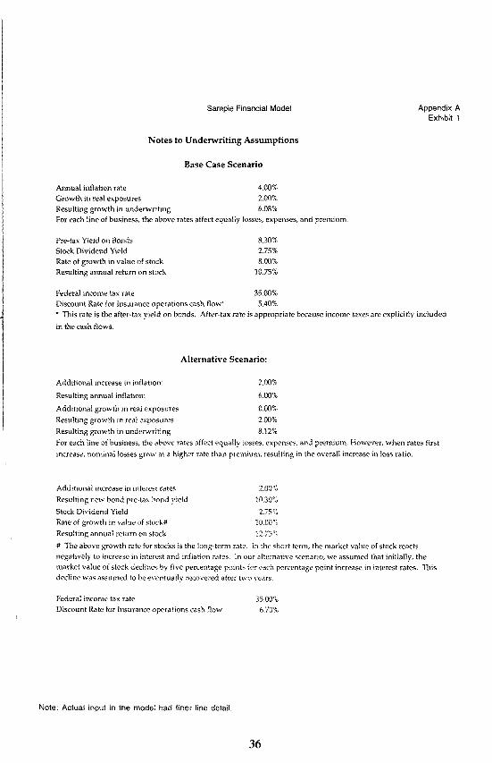
SamDie Financial Model Appendix A Exhibit 1

Notes to Underwriting Assumptions

Base Case Scenario

Annual inflation rate 4.00% Growth in real exposures 2.00% Resulting growth in underwriting 6.08% For each line of business, the abovc rates affect equally losses, expenses, and ~remiutn.

Pretax Yield on Bonds 8.30% Stock Dividend Yield 2.75% Rate of growth in value of stock 8.007 0 Resulting annual return on stock 10.75%

Federal income tax rate 35.00% Discount Rate for Insurance operations cash flow’ 5.40% * This rate is the after-tax yield on bonds. After-tax rate is appropriate because income taxes are explicitly mcluded

in the cash flows.

Alternative Scenario:

Additional mcrease in inflation: 2.00%

Resulting annual inflation: b.OO’Y D

Additional growth in real exposures 0.00% Resulting growth m real exposures 2.00’% Resulting growth m underwriting 8.12% For each line of business, the above rates affect equally losses, crpcnscs, and premium. However, when rates first mcrease, nominal losses grow at a higher rate than prenxum, resulting m the overall mcrease in loss ratio.

Additional increase m mtercst rates 2.00” G Resultmg new bond FE-tax bond yield 10.30% Stock Diwdend Yield 2.751 0 Rate of growth in value of stock# 10 00”; Resulting annual return on stock 12 Z”,,

# J’he above growth rate for stocks is the long-term rate In thr short term, the market value of stock reacts negatively to increase m interest and inflation rates. In our alternahre scenarm, we assumed that mitially, the market value of stock declines by five percentage pomts for each percentage point increase m interest rata. This decline was assumed to be eventually rccovcred after tn-o years

Federal income tax rate 35.00”” Discount Rate for Insurance operations cash flow 6.70%

Note: Actual input in the model had finer line detail.

36

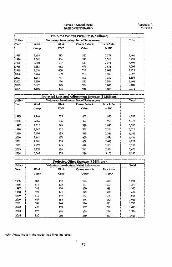
Sample Financial Model Appendix A BASE CASE SCENARIO Exhibit 2

Voluntary, Involuntary, Net of Reinsurance Work GL& Comm Auto & Pers Auto

Comp CMP &HO

2,415 513 562 2,374 2,562 544 596 2,518 2,718 577 633 2.671 2,883 612 673 2,834 3,058 650 712 3,006 3,244 689 755 3,189 3,441 731 801 3,382 3,650 776 850 3,588 3,872 823 902 3,806 4,108 873 956 4,038

Total

5,864 6,220 6,599 7,000 7,425 7,sn 8,356 8,864 9,403 9.974

t

1 Projected Loss and Adjustment Expense ($ Millions)

Voluntary, Involuntary, Net of Reinsurance Work GL& Comm Auto & Pen Auto

camp CMP Other &HO

1,966 505 462 1,855

2,086 535 490 1,968

2,212 5M) 520 2,087 2.347 602 551 2,214 2,490 639 585 2,349 2,641 678 620 2,491 2,801 719 658 2,643 2,972 763 698 2,804 3,152 809 741 2,974 3,344 656 786 3,155

Total

4,787

5,078

5,387 5,7l5 6,062 6,431 6,822 7,236 7,676 8,143

Projected Other Expense ($ Millions) Voluntary, Involuntary, Net of Reinsurance

Work GL& Comm Auto & Pers Auto

482 118 511 125 542 133 575 141 610 149 647 158 687 lb8 728 178 773 189 820 201

CMP Other &HO

124 478 131 507 139 538 148 570 157 605 166 642 176 681 187 722

198 766

210 813

Total

I 1,201 1,274 1,352 1,434 1,521 1,613 1,711 1,815

1,926

2,043

1

Note: Actual input in the model had finer line detail

37

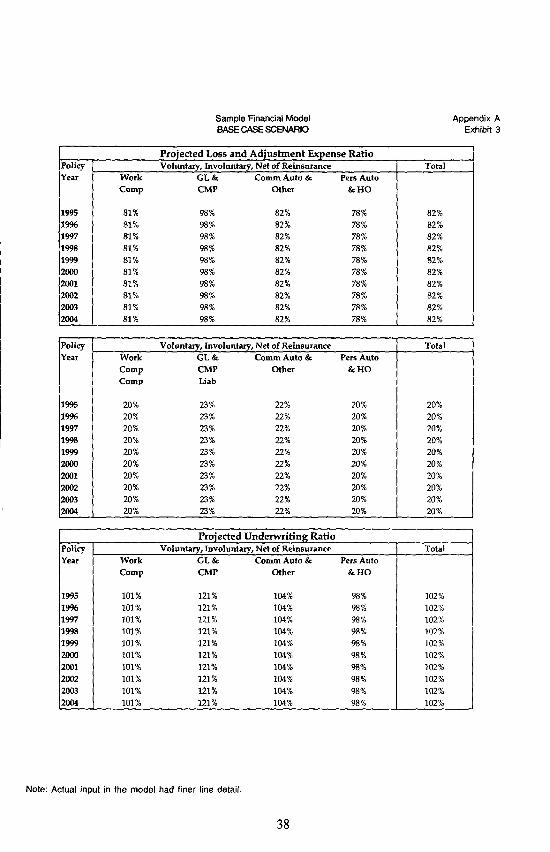
Sample Financial Model BASE CASE SCENARIO

Appendix A Exhibit 3

81% 81% 81% 81% 81% 81% 81% 81% 81% 81%

CMP Other &HO -I

Projected Loss and Adjustment Expense Ratio Voluntary, Involuntary, Net of Reinsurance

Work GL& Comm Auto & Pers Auto

98% 82% 98% 82% 98% 82% 98% 82% 98% 82% 98% 82% 98% 82% 98% 82% 98% 62% 98% 82%

78% 78% 78% 78% 78% 78% 78% 78% 78% 78%

Voluntary, Involuntary, Net of Reinsurance Work GL& Comm Auto & Pers Auto Camp CMP Other &HO Camp Liab

20% 23% 20% 23% 20% 23% 20% 23% 20% 23% 20% 23% 20% 23% 20% 23% 20% 23% 20% 23%

22% 20% 22% 20% 22% 20% 22% 20% 22% 20% 22% 20% 22% 20% 22% 20% 22% 20% 22% 20%

Comp CMP

Total

82% 82% 82% 82% 82% 82% 82% 82% 82% 82%

Projected Underwriting Ratio Voluntary, Involuntary, Net of Reinsurance

Work CL& Comm Auto & Pers Auto &HO

Total

20% 20% 20% 20% 20% 20% 20% 20% 20% 20%

98% 98% 98% 98% 98% 98% 98% 98% 98% 98%

Total

Note: Actual input in the model had finer line detail.

38

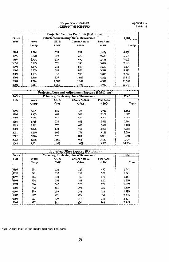
Sample Financial Model Appendix A AL-IERNATIVE SCENARIO Exhibit 4

Projected Written Premium ($ Millions) Voluntary, Involuntary, Net of Reinsurance

Work GL& Comm Auto & Pers Auto Camp CMP Other &HO Comp

2,514 534 589 2,421 6,058 2,720 578 637 2,620 6,555 2,944 625 690 2,835 7,093 3,185 676 746 3,067 7,675 3,446 732 807 3,319 8,304 3,729 792 874 3,591 8,985 4,035 857 945 3,885 9,722 4,366 927 1,023 4,204 10,519 4,724 1,003 1,107 4,549 11,382 5,111 1,085 1,198 4,922 12,316

-r Total

I Projected

1 Voluntary, Involuntary, Net of Reinsurance 1

Work GL& Comm Auto & Pm Auto Comp CMP Other &HO

2,175 562 496 1,949 2,353 608 536 2,109 2546 658 580 2,282 2,755 712 628 2,469 2,981 770 680 2,672 3,w 834 735 2,891 3,490 902 796 3,128 3,776 976 861 3385 4,086 1,056 931 3,662 4,421 1,143 l,o+lS 3,963

Total

camp

5,182 5,607 6.067 6,564 7,103 7,685 8,316 8,9!% 9,736 10,534

Projected Other Expense ($ Millions) Voluntary, Involuntary, Net of Reinsurance I

Work GL& Camm Auto & Pers Auto Comp CMP Other &HO

501 122 129 490 541 132 139 529 586 143 150 573 634 154 163 620 686 167 176 671 742 181 190 726 803 195 206 785 869 211 223 850 933 229 241 918 979 243 256 968

Total

Comp

1,241 1341 1,451 1,570 1,699 1,839 1,989 2,153 2,321 2,445

Note: Actual input in the model had finer line detail

39

Sample Financial Model ALTERNATIVE SCENAFflO

Appendix A Exhibit 5

Projected Loss and Adjustment Expense Ratio Voluntary, Involuntary, Net of Reinsurance

Work GL& Comm Auto & Pets Auto Comp CMP Other &HO

87% 87% 87% 87% 87% 87% 87% 87% 87% 87%

105% 84% 81% 105% 84% 81 % 105% 84% 81% 105% 84% 81% 105% 84% 81% 105% 84% 81% 105% 84% 81% 105% 84% 81% 105% 84% 81% IO.57 0 84% 81%

Voluntary, Involuntary, Net of Reinsurance Work GL& CommAuto& Pers Auto COIIIQ Comp

CMP Liab

Other &HO

20% 23% 22% 20% 20% 23% 22% 20% 20% 23% 22% 20% 20% 23% 22% 20% 20% 23% 22% 20% 20% 2376 22% 20% 20% 23% 22% 20% 20% 23% 22% 20% 20% 23% 22% 20% 19% 22% 27% 20%

Total

86% 86% 86% 86% 86% 86% 86% 86% 86% 869 0

Total

Camp

20% 20% 20% 20% 20% 20% 20% 20% 20% 20%

Projected Underwriting Ratio Voluntary, Involuntary, Net of Reinsurance

Work GL& Comm Auto & Pers Auto t Comp CMP Other &HO

106% 106% 106% 106% 106% 106% 106% 106% 106% 106%

128% 128% 1289 0 128% 128% 128% 128% 128% 128% 128%

106% 106% 106% 106% 106% 106% 106% 106% 106% 105%

101% 107 % 101% 101% 101% 101% 101% 101% 101% 100%

Total

I 106% 106% 1067 " 106% 106% 106% lob% 105%

1

Note: Actual input in the model had finer line detail.

40

Sample Financial Model Appendix B Exhibit 1

Market Value of Mortgage Backed Securuites

1 , , I f

I i I I

New Rates and new pattern I I / I I I 1 I / / ,

/

New Rates but old pattern

Difference is the result of motgage holders 1 pre-paying at a slower rate, as a result of the /

higher interest rates. I ! I

I I ,

I I

I I

/ /

Base case

5,700 5,800 5,900 6,000 6,100 6,200 6,300 6,400 6,500 6,600

Value in Millions

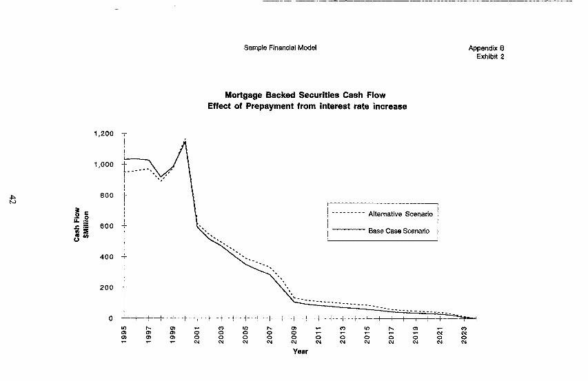
Sample Financial Model Appendix 0 Exhibit 2

1,200

1,000

800

600

400

200

0

Mortgage Backed Securities Cash Flow Effect of Prepayment from interest rate increase

I --------- Alternative Scenario

i Base Case Scenario

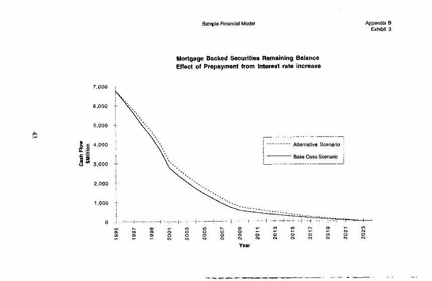
Sample Financial Model Appendix B Exhibit 3

7,000

6,000

5,000

g E 4,000 E 0 rz 03 0 3,000

2,000

1,000

0

Mortgage Backed Securities Remaining Balance Effect of Prepayment from interest rate increase

-.

Sample Financial Model Appendix B Exhibit 4

Total Fixed Income Securities Cash Flow Effect of Prepayment from interest rate increase

--------- Alternative Scenario

Base Case Scenario

Year

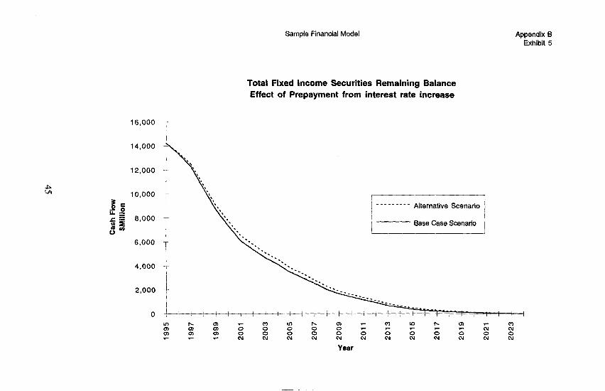
Sample Financial Model Appendix I3 Exhibit 5

16,000

14,000

12,000

4,000

2,000

0

‘. \

\

*. ‘.

*\

-t

Total Fixed Income Securities Remaining Balance Effect of Prepayment from interest rate increase

/ 3 1 --------- Alternative Scenario ! I / j - Base Case Scenario I

Year

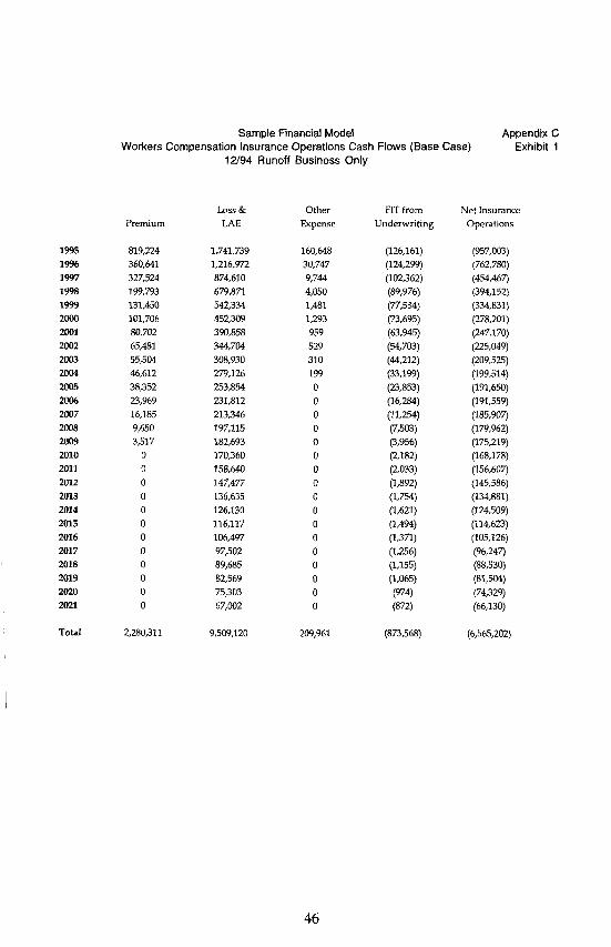
1995 819,224 1,741,739 160,648 (126,161) 1996 360,641 1,216,972 30,747 (124,299) 1997 327,524 874,610 9,744 (102,362) 1998 199,793 679,871 4,050 (89,976) 1999 131,450 542,334 1,481 (77,534) 2000 101,706 452,309 1,293 (73,695) 2001 80,702 390,858 959 (63,945) 2002 65,481 344,704 529 (54,703) 2003 55,504 308,930 310 (44,212) 2004 46,612 279,126 199 (33,199) 2005 38,352 253,854 0 (23,853) 2006 23,969 231,812 0 (16,284) 2007 16,185 213,346 0 (11,254) 2008 9,650 197,115 0 (7,503) 2009 3,517 182,693 0 (3,956) 2010 0 170,360 0 (2,182) 2011 0 158,640 0 (2.033) 2012 0 147,477 0 (1,892) 2013 0 136,635 0 (1,754) 2014 0 126,130 0 (1,621) 2m5 0 116,117 0 (1,494) 2016 0 106,497 0 (1,371) 2017 0 97,502 0 (1,256) 2018 0 89,685 0 (1,155) 2019 0 82j569 0 (1,065) 2020 0 75,303 0 (974) 2021 0 67,002 0 (872)

Total 2,280,311 9,509,120 209,961 (873,568)

Sample Financial Model Workers Compensation Insurance Operations Cash Flows (Base Case)

12/94 Runoff Business Only

Appendix C Exhibit 1

Loss & LAE

Other Expens

FIT from Underwriting

Net Insurance Operations

(957,003) (762,780) (454.467) (394,152) (334,831) (278,201) (247,170) (225,049) (209,525) (199,514) (191,650) (191,559)

(185,907) (179,962) (175,219) (168,178) (156,607) (145,586) (134,881) (124,509) (114,623) (105,126) (96,247) (88,530)

@VfY (74,329) (66,130)

(6,565,202)

46

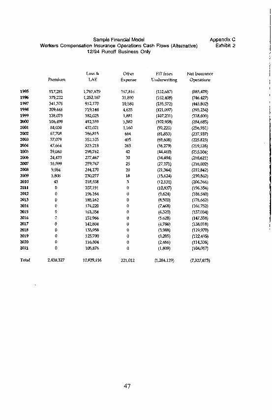
1995 917,281 1,767,629 167,816 (132,687) 19% 375,222 1,252,167 31,890 (162,408) 1997 341,376 912,170 10,580 (135572) 1998 209,446 n9s44 4,633 (mo97) 1999 138,075 582,025 La81 (107,231) 2004 106,499 492,559 1,582 (102,958) 2001 84,030 432,021 1,160 (92,220) 2002 67,708 386,815 664 (81,833) 2003 57,079 352,105 405 (69,608) 2004 47,664 323,218 263 (56,279) 2005 39,040 298,762 42 (44,460) 2006 24,473 277,467 30 (34,404) 2007 16,599 259,747 25 (27,171) 2008 9,984 244,170 20 (21364) 2009 3,808 230,277 18 (15,624) 2010 43 218,538 3 (12,131) 2011 0 207,191 0 (10,837) 2012 0 196,164 0 (9,624) 2m3 0 185,162 0 (8,500) 2m4 0 174,220 0 (7,468) 2015 0 163.554 0 (6520) 2016 0 152,966 0 (5,628) 2017 0 142,804 0 (4.786) 2m8 0 133,958 0 (3,988) 2019 0 125,700 0 (3,205) 2020 0 116,804 0 (2,466) 2021 0 105,876 0 (lim)

Total 2,438,327 10,829,116 221,012 (1,284,129)

Sample Financial Model Workers Compensation Insurance Operations Cash Flows (Alternative)

12/94 Runoff Business Only

Appendix C Exhibit 2

Premium Loss &

LAE Other

Expense FIT from

Underwriting Net Insurance

OpeEbXlS

(885,478) (746,427) (445,802) (393,234) (338,600) (284,685) (256,931) (237,937) (225,823) (219,538) (215,304) (218,621) (216,002) (212,842) (210,862) (206,366) (196,354) (186,540) (176,662) (166,752) (157,034) (147,338) (138,018) (129,970) (122,@5) (114,338)

(104,067)

(7X7,673)

47

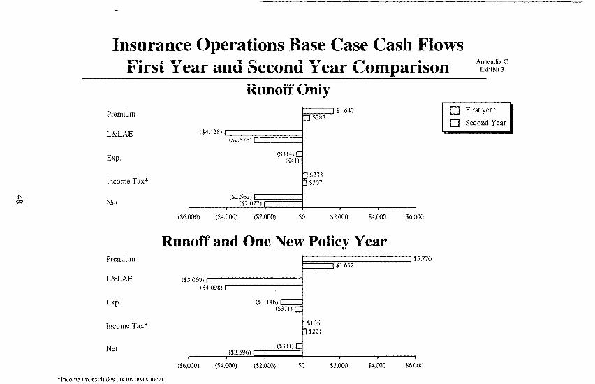
Insurance Operations Base Case Cash Flows First Year and Second Year Comparison Appendix C

Exhibit 3

L&LAE

Exp.

Income Tax”

Net

Runoff Only

($4,128) 1 (52,576) r

-J 5233 I$207

($2.562) r

r ($2,027) f

I ($6.000) ($4.000) ($2.000) $0 $2.000 $4.OJM $6,000

Runoff and One New Policy Year Premium

L&LAE

EXP

Income Tax*

Net ($33 I ) ($2,596) I

r #

($6,000) ($4,ow (s2.000) $0 $2,000 $4,000 $6,000

[23 First year

[3 Second Year I

Insurance Operations Cash Flow in First Year *%Z,T Base Case

Premium

L&LAE

one new year

Exp.

Income Tax*

Net

($6,000) ($4,ooO) ($2,ooO) $0 $2,000 woo0 $6WQ $8,000

Alternative Scenario Premium

L&LAE

Exp.

1$1,795 -1 $6,048

($4,202) ($5,152) ) .. ~!. .-.i m~.u-.c~&..:.

(%324)C ($1,182)=

Income Tax* -J$264 ]$I19

Net ($2,468) \ ($167) , 1

($6,000) ($4,000) ($2,000) $0 $ZW $4,000 $6,ooO $8,000

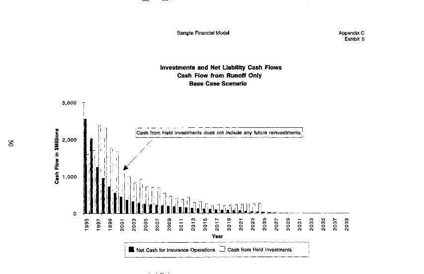
Sample Financial Model Appendix C Exhibit 5

3,000

e

: 2,000 z Y) .E

z C

5 1,000 J

0

Investments and Net Liability Cash Flows Cash Flow from Runoff Only

Base Case Scenario

Cash from Held investments does not include any future reinvestments.

/

Year

’ n Net Cash for Insurance Operations m Cash from Held Investments I 1

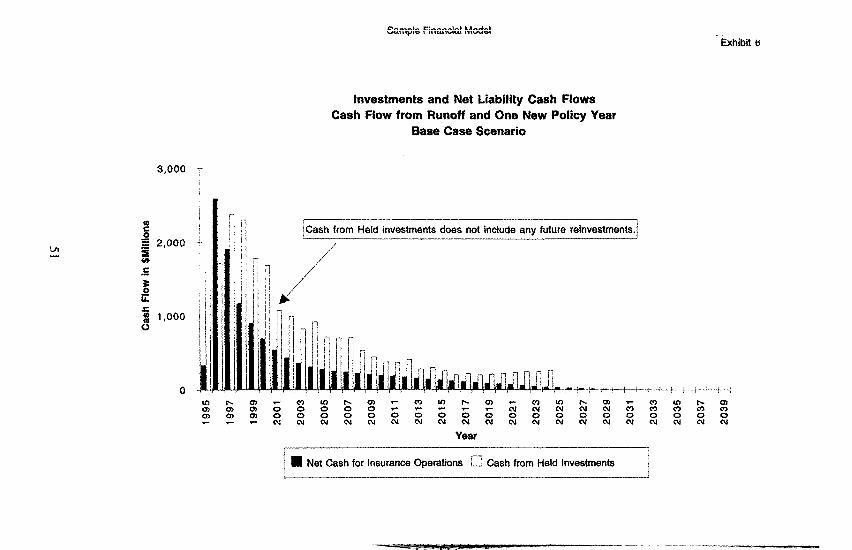
Sample Financial Model Exhibit 6

Investments and Net Liability Cash Flows Cash Flow from Runoff and One New Policy Year

Base Case Scenario

3,000 7

I e g 2,000 L z 5

k ii.

f 1,000 + d

I

0 r

/Cash from Held investments does not include any future reinvestments.

il/

m Net Cash for insurance Operations a Cash from Held Investments I i

Sample Financial Model Appendix C Exhibit 7

Investments and Net Liability Cash Flows Cash Flow from Runoff Only

Alternative Scenario

3,000

,--~--I- ______--- ___-_____ Cash from Held investments does not include any future reinvestments.:

Year --- __-

( n Net Cash for Insurance Operations 1 Cash from Held Investments

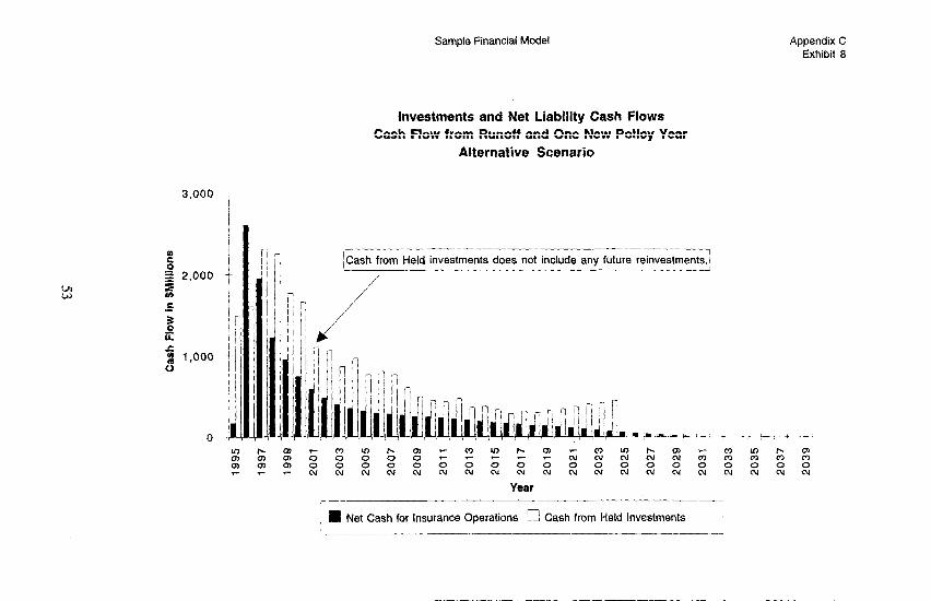
Sample Financial Model Appendix C Exhibit 8

Investments and Net Liability Cash Flows Cash Flow from Runoff and One New Policy Year

Alternative Scenario

3,000 i

.r

jCash from Held investments does not include any future reinvestments.:

1 n Net Cash for Insurance Operations E Cash from Held Investments I

;

Sample Financial Model

Net cash flows under the two Scenarios Cash Flow from Runoff Only

Yearly cash for base case _ _ _ - - - - - - Yearly cash for alternative scenario j

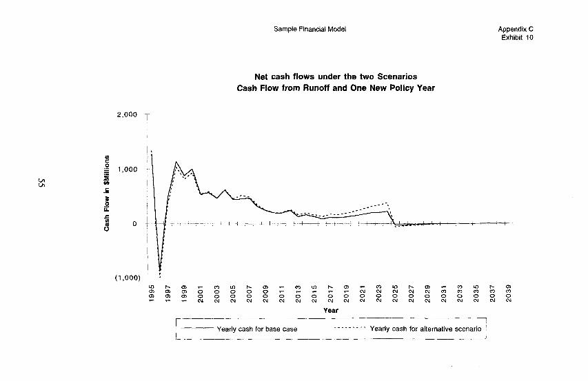
Sample Financial Model Appendix C Exhibit 10

.E

b t c 2 0

Net cash flows under the two Scenarios Cash Flow from Runoff and One New Policy Year

2,000 ,

1,000

0

r -~-- _________~. Yearly cash for base case

Year

- - - - - _ --- Yearly cash for alternative scenario

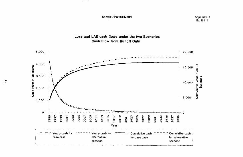
Sample Financial Model Appendix C Exhibit 11

Loss and LAE cash flows under the two Scenarios Cash Flow from Runoff Only

5,000 i 20,000

e 4,000

.g

.Z w 3,000 .c

3 k 2,000 f J

1,000

Yearly cash for _ _ - _ _ _ _ . Yearly cash for Cumulative cash - - - - - Cumulative cash base case alternative for base case for alternative

scenario scenario -~~~ _I___ J

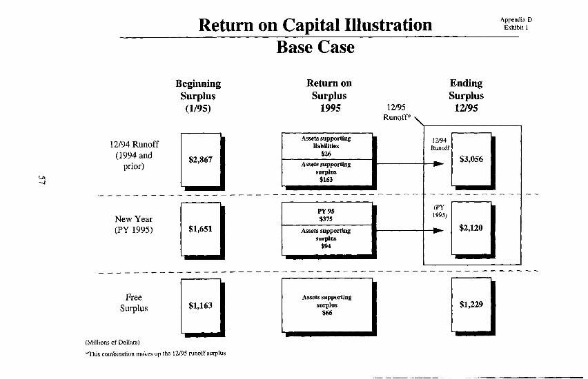
Return on Capital Illustration - Appendix D

Exhibit I

12194 Runoff (1994 and

prior)

--

New Year (PY 1995)

Free Surplus

Base Case

Beginning Surplus (l/95)

Return on Surplus

1995

Assets supporting

liabilities

$26 t----l Assets supporting

SUrplUS

$163

Ending Surplus

Runoff*

$3,056

$1,651 I w 1995)

--

Assets supporting

surplus

$66

$1,229

(Millions of Dollars)

*This combination makes up the 12/95 runoff surplus

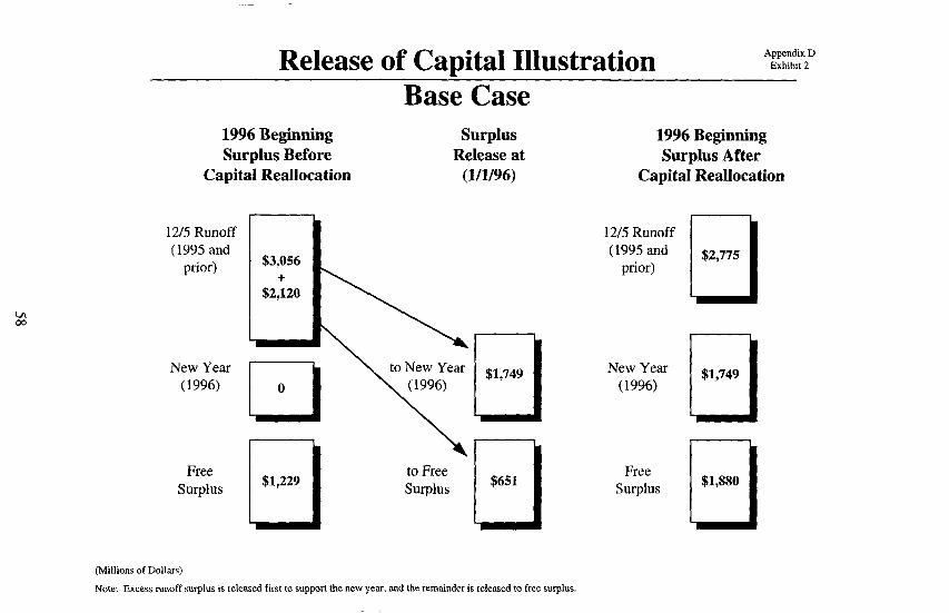
Release of Capital Illustration Appendix D Exhibit 2

Base Case 1996 Beginning Surplus Before

Capital Reallocation

Surplus Release at

(l/1/96)

1215 Runoff (1995 and

prior)

New Year (1996)

Free Surplus

1996 Beginning Surplus After

Capital Reallocation

(Millions of Dollars)

Note: Excess runoff surplus is released first to support the new year, and the remainder is released to free surplus.

12/5 Runoff (1995 and

prior) $2,775

New Year (1996)

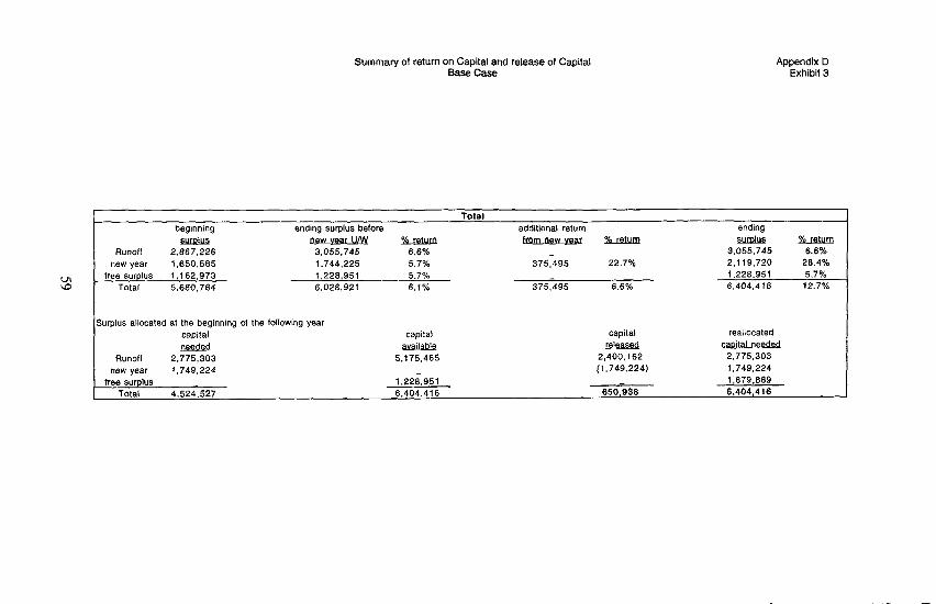
Summary of return on Capital and release of Capital Base Case

Appendix D Exhibit 3

total beginning ending surplus before additional return ending

as!u!b mw war UP& - -new Fllmlus - Runoff 2.667,226 3.055,?45 6.6% 3,055,745 6.6%

new year 1,650,565 1.744,225 5.7% 375.495 22.7% 2.119.720 26.4% free surplus 1.162.973 1.226.951 5.7% 5.7%

Total 5660.764 6.026,921 6.1% 375,495 1.226.951

6.6% 6.404.416 12.7%

Surplus allocated at the beginning of the following year capital

Runoff 2.775.303

Capital capital

ab!Eg&k rrrlaaseri 5175.465 2,400,162

reallocated

2,775.303

new year 1;749:224 1,749,224

free surplus 4,52<527

1.228.951

(1,749,224) 1.679.669

Total 6,404,416 650,936 6,404,416

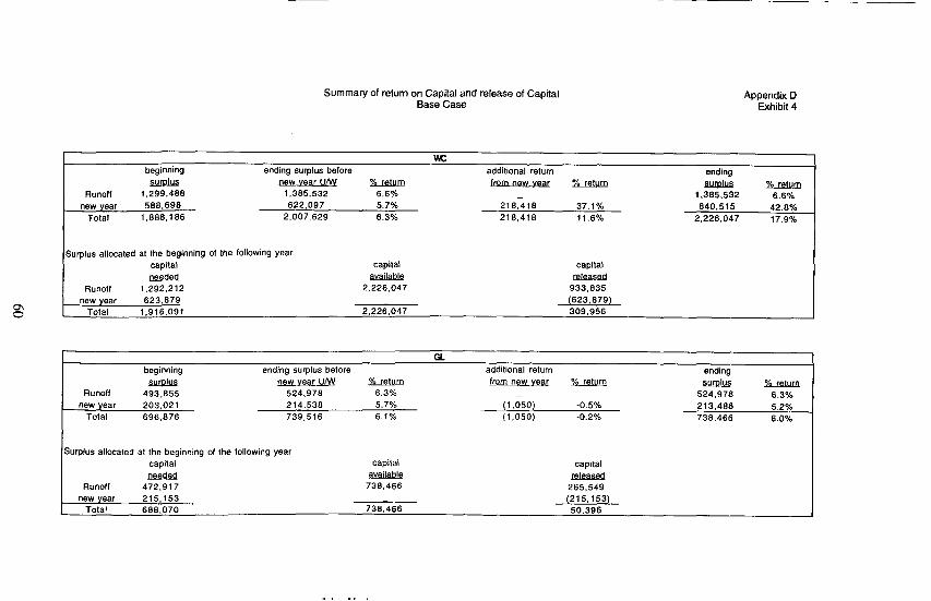
Summary of return on Capital and release of Capital Base Case

Appendix 0 Exhibit 4

w

beginning ending surplus before additional return ending new vear UPA! l?LL&um from- -

Runoff 1.299.466 1.365.532 6.6% 1.365,532 6.6%

new year 566,696 622,097 5.7% 216316 37.1% 640,515 42.6%

Total 1.666,166 2.007.629 6.3% 216,416 11.6% 2,226,047 17.9%

Surplus allocated at the beginning of the following year capital

oaadad Runoff 1.292.212

new year 623,679 Total 1.916.091

capiial

ay&&lQ 2.226,047

2.22i.047

capital

- 933,635 (623,679) 309,956

u

beginning ending surplus before additional return ending

sur!JhE new vear Uffl - from new year &..r.&m E%ttn!u ?k.LQum Runoff 493,655 524.976 6.3%

(1.050) 524,976 6.3%

new year 203,021 214,536 5.7% -0.5% 213.466 5.2% Total 696,676 739,516 6.1% (1,050) -0.2% 736,466 6.0%

Surplus allocated at the beginning of the following year capital

JIQBW Runoff 472,917

capital ay&&

736,466

capital

265,549 new year 215,153 (215,153)

TOW 666,070 736,466 50,396

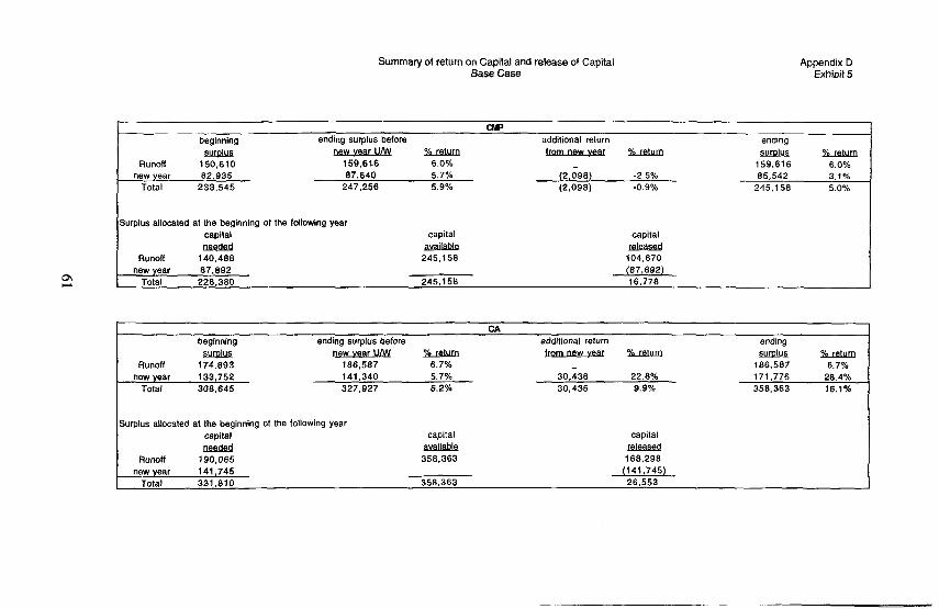
Summary of return on Capital and release of Capital Base Case

Appendix D Exhibit 5

cm

beginning ending surplus before additional return ending

oew ?!Lreim -new ?LLcQuQ Runoff 150,610 159,616 6.0%

new year 82,935 87,640 5.7% (2.;98) 159,616 6.0%

-2.5% 85,542 3.1% Total 233,545 247,256 5.9% (2,096) -0.9% 245,156 5.0%

Surplus allocated at the beginning of the following year

capital

Runotf 140.488

new year 87.092 Total 228.380

capital

- 245,158

245; 58

capital

104.670 (87,892) 16,778

Runoff new year

Total

beginning

174,893 133,752 308,645

CA ending surplus before additional return ending

new Y!izaum foxn new ymr % return %..mLm 186,587 6.7% 186,587 6.7% 141,340 5.7% 3O,i36 22.8% 171.776 28.4% 327,927 6.2% 30,436 9.9% 358,363 16.1%

Surplus allocated at the beginning of the following year capital

oee.dad Runoff 190,065

new year 141,745 Total 331,810

capital

- 358.363

358.363

capital

168,298 (141,745)

26,553

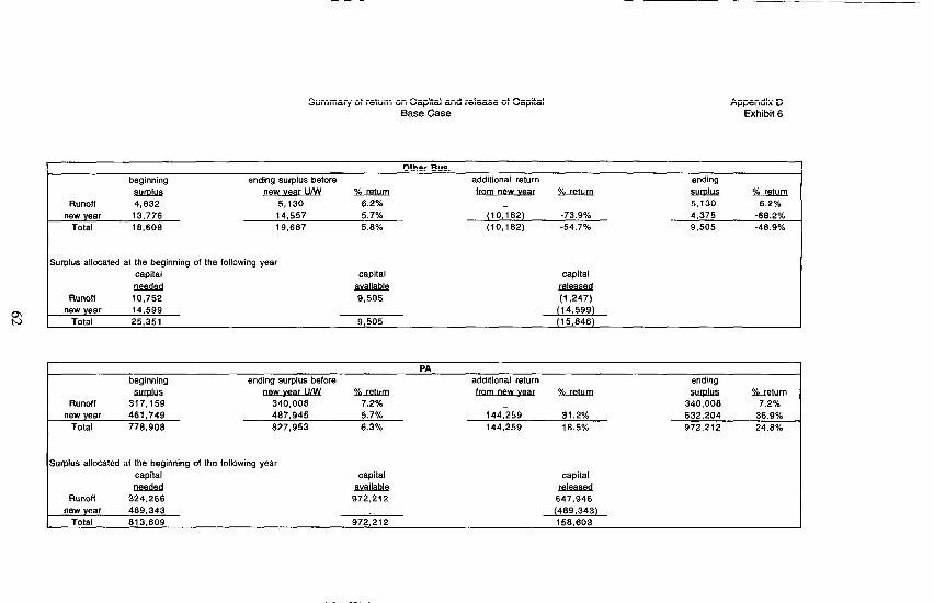
Summary of return on Capital and release of Capital Appendix D Base Case Exhibit 6

Other Bus. beginning ending surplus before additional return ending

svlplus new ?!Qmhlm from- YL.mml Runoff 4.832 5.130 6.2% 5.130 6.2%

14,557 5.7% - 19,687 5.8%

(10,182) -73.9% (10,182) -54.7%

41375 -68.2% 9,505 -48.9%

Surplus allocated at the beginning of the following year capital

Runoft 10,752 new year 14,599

Total 25,351

capital

8.YAwle 9,505

9,505

capital

(1,247) (14,599) (15,848)

beginning ending surplus before additional return ending flew Year UN - from- s!4tP.b -

Runoff 317,159 340,008 7.2% 340,008 7.2%

487,945 5.7% 144,259 31.2% 632,204 36.9% 827,953 6.3% 144,259 18.5% 972.212 24.8%

Surplus allocated at the beginning of the following year capital

naada Runoft 324,266

capital

ElYabuQ 972,212

capital

- 647,946

new year 489,343 (469,343) Total 813.609 972,212 158,603 I

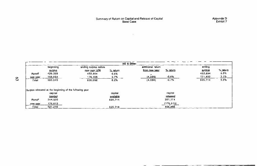
Summary of Return on Capital and Release of Capital Appendix D Base Case Exhibit 7

HO 6, Other beginning ending surplus before additional return ending

t.?luRb new vex UMI IYLrawa -new ycplus ?!iJQtm Runoff 426,389 453,894 6.5% 453,694 6.5%

new year 166,654 176,108 6.2% 5.7% (4,288)

Total 593,043 630,002 (4,288) -0.7% -2.6% 625.714 171,820 5.5% 3.1 %

5urplos allocated al the beginning of the following year

capital

tEedad Runoff 344,603

new year 176,613 Total 521,216

capital

- 625,714

625314

capital

reiaasarl 281,111

(176,613) 104.498

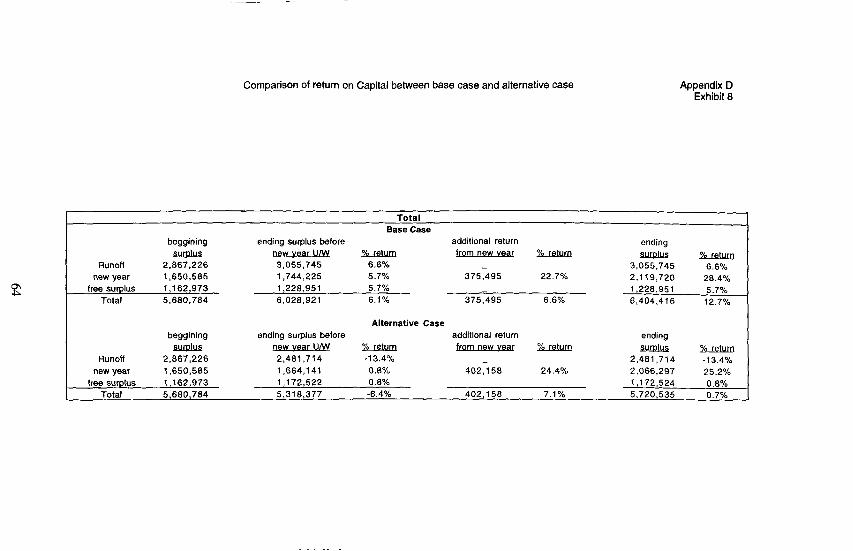
Comparison of return on Capital between base case and alternative case Appendix D Exhibit 8

Runoff new year

beggining

2.867,226 1,650,585

Total Base Case

ending surplus before additional return ending new v*ar UNV ?!Lceml tom new VW w - 3,055,745 6.6% 3,055,745 6.6% 1.744,225 5.7% 375,495 22.7% 2,119,720 28.4% 1,228,951 5.7% 6,028,921 6.1% 375,495

Runoff new year

free surplus Total

beggining

2,867,228 7,850,585 I ,162,973 5,680,784

Alternative Case ending surplus before additional return ending

oew ?ILxmuo from new veilc % return zzua!ds - 2D487.774 -73.4%

402: 58 2,481,714 -13.4%

7,684,141 0.8% 24.4% 2,068,297 25.2% 1,172,522 0.8% 1,172,524 0.8% 5,318,377 -6.4% 402.158 7.1% 5,720,535 0.7% _

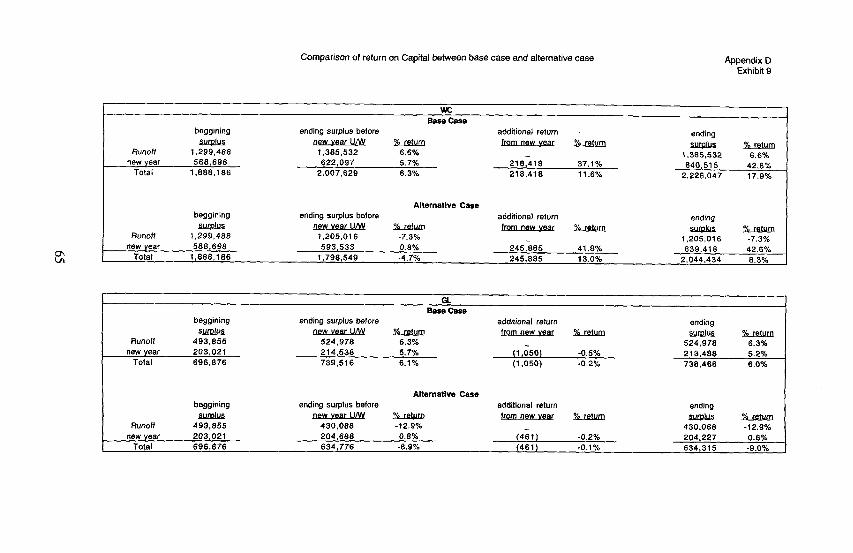
Comparison of return on Capital between base case and alternative case Appendix D Exhibit 9

beggining ending surf~lus before

s!J@4s oew z!-zdam Runoff 1.299.488 13385.532 6.6%

new year 588,698 622,097 5.7% 218.418 37.1% 42.8% TOtal

840,515 1,886.186 2.007.629 6.3% 218,418 11.6% 2,226,047 17.9%

Alternative Case beggining ending surplus before

s.ia!IE new - Runoff 1.299.488 1.205,016 -7.3%

additional return

-new

ending

zLLL&Ko 1.385.532 6.6%

additional return ending -new svrplus Tk.Ja!m

1.205.016 -7.3% new year 588,698 593,533 0.8%

t2 Total 1,888.186 1.798,549 -4.7% 245,865 245,885 41.8% 13.0% 2.044.434 839,418 42.6% 8.3%

Runoff new year

Total

beggining

!2lLc&2 493,855 203,021 696,876

a Base case

ending surplus before additional return ending oew z4-rs&n fr.Qm “SW ma r4hcetum §!ami yQLeuL0

524,978 6.3% (1 .oso,

524,978 6.3% 214,538 5.7% -0.5% 213,488 5.2% 739,516 6.1% (1.050) -0.2% 738,486 6.0%

RU”O!f new year

Total

beggining

493,855 203,021 696,876

Alternative Case ending surplus before addiiional return ending

new !T6l&ro -new fil!m!m - 430,088 -12.9%

(461) 430,088 -12.9%

204,688 0.8% -0.2% 204,227 0.6% 634,776 -8.9% (461) -0.1% 634,315 -9.0%

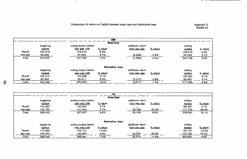
Comparison of return on Capital between base case and alternative case Appendix D Exhibit IO

Runoft new year

Total

beggining

surplus 150,610 82,935

233,545

Runoff

beggining

svrplus 150,610

ending surplus before

new !cQauLn 159,616 6.0% 87,640 5.7%

247,256 5.9%

Alternative Case ending surplus before

new T!YumKo 136,968 -9.1%

additional return

from-

(2,&8) -2.5%

(2,098) -0.9%

ending

ylrplus k!kaAMO 159,616 6.0% 85,542 3.1%

245,158 5.0%

additional return ending from- surnlus z4-wum

136,968 -9.1%

new year 82,935 83,617 0.8% (3,217) -3.9% 80,400 -3.1% 22 Total 233,545 220,585 -5.5% (3.217) -1.4% 217,368 -6.9%

CA Base Case

I baggining ending surplus before additional return ending

I sJGl!a- new zL?xmm -new ?L!mlG T&.LQul

Runoff 174.893 186.587 6.7% 166.587 6.7% new year 133;752

Total 308.645

141;340

327.927

5.7%

6.2% 30,436 22.8% 171;776 28.4% 30,436 9.9% 358,363 16.1%

RU”Ofl new year

Total

beggining

suozlus 174,693 133,752 308,645

Alternative Case ending surplus before additional return ending

new !h-mkla m new “*a m sYuQi!s z!%Lwum 152,101 -13.0%

35,870 152,101 -13.0%

134,850 0.8% 26.8% 170,720 27.6%

286,951 -7.0% 35,870 11.6% 322,821 4.6%

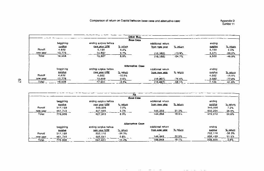
Comparison of return on Capital between base case and alternative case Appendix D Exhibit 11

Other Bus. Base Case

I beggining ending surplus before w war Q& yQL?m

Runoff 4.632 5.130 6.2% 14,557 5.7% 19,687 5.8%

beggining

svrplus 4,832

Alternatlvs Case ending surptus belore

oew z!dQbdm 4,062 -15.9%

additional return

tromnewvear I?!LEam

(tO.l82) -73.9%

(10.182) -54.7%

ending

5,130 4,375 9,505

ghrefvrn 6.2%

-68.2% -48.9%

additional return ending

-new Ysm2!@ - 4,062 -15.9%

5 new Total year 13,776 13,869 -3.5% 0.8% (7o,ao7) -78.4% 3,082 -77.6%

18,608 17,951 (10.807) -58.1% 7.144 -61.6%

PA Ease Casa

beggining ending surplus before additional return ending

zJJ.mb m - fromnew 2%!da!s %x!bm Runoff 317,159 340,008 7.2% 340,008 7.2%

new year 461,749 487,945 5.7% 144,259 31.2% 632,204 36.9% Total 776,908 827,953 6.3% 144,259 16.5% 972,212 24.6%

RU”Off new year

Total

beggining

i5.tmb 317,159 461,749 778,908

Alternative Case ending surplus before additional return ending

!l?cdan tromnew 2%uB!Ys !4sIuul 202,110 -36.3% 202,110 -36.3% 465,541 0.8% 140,949 30.5% 606,490 31.3% 667,651 -14.3% 140,949 18.1% 808,600 3.8%

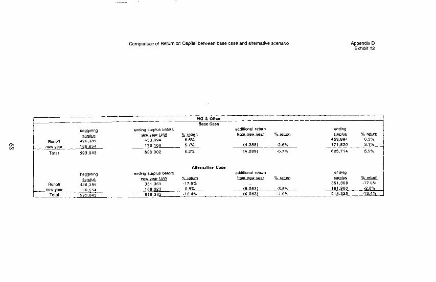
Comparison of Return on Capital between base case and alternative scenario Appendix D Exhibit 12

Runoff new year

TOElI

beggining

ctut!G 426,389 166,654

593,043

HO 8 Other Ease Case

ending surplus before additional return ending new war urn Q.&g from new vex ?Lc&r~ s!JaLLs n

453,694 6.5% 6.5% 176.106 5.7% (4.288)

453,694 -2.6% 171,820 3.1%

630.002 6.2% (4.288) -0.7% 625.714 5.5%

Runoff new year

TOhI

beggining

2Lurms 426.369 166,654 593,043

Alternative Case

ending surplus before additional return ending new war u/w y&.&K0 from new veaf YdeUr13 suD!us m

351,369 -17.6% 351,369 -17.6% 168,023 0.6% (6,063) -3.6% 161,960 -2.8%

519,392 -12.4% (6,063) -1 .O% 513,329 -13.4%

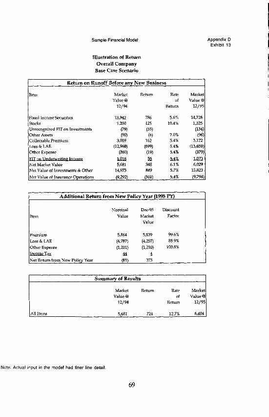
Sample Financial Model Appendix D Exhibit 13

Illustration of Return Overall Company

Base Case Scenario

I Return on Runoff Before any New Business

item Market Value @I

12194

Return Rate Market of Value 0

Return 12195

Fixed income Securities Stocks Unrecognized FIT on Investments Other Assets Collectable Premium Loss & LAE Other Expense

Net Market Value Net Value of Investments &Other

Net Value of Insurance Op WdiOIlS

13,942 1,200

(79) m

(lag,

(360) lsm 5,681

14,973

(9,292)

786 125

(55) (6)

162

(699) (19) 55

348 849

W)

5.6% 10.4%

7.0% 5.4% 5.4% 5.4%

5.&h 6.1% 5.7%

5.4%

Additional Return from New Policy Year (1995 PY)

Item Nominal

Value Dee-95 Discount Market Factor

Value

Premium Loss & LAE Other Expense

Net Return from New Policy Year

5,864 5,839 99.6%

(4,787) (4,257) 88.9%

(1,201) (1,210) 100.8%

&4 4

(81) 375

Summary of Results 1

Market Value Q

12194

R‘Zhll7l Rate of

Return

Market Value 0

12195

All Items 5,681 724 12.7% 6,404

Note: Actual input in the model had finer line detail

69

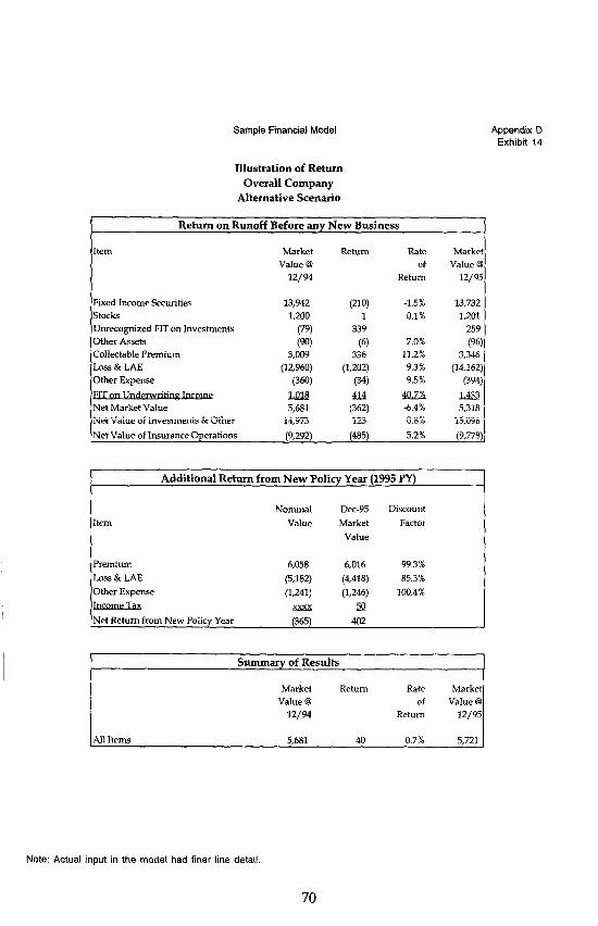
Sample Financial Model Appendix D Exhibit 14

Illustration of Return Overall Company

Alternative Scenario

Return on Runoff Before any New Business

km

Fixed Income seturities stocks Unrecognized FIT on Investments Other Assets Collectable Premium Loss & LAE Other Expense

Net Market Value Net Value of Inveshnents &Other

Net Value of Insurance Operations

Market Value @

12/94

13,942 1,200

(79) w9

3.w9 (12,960)

(360) l‘Ql8 5,681

14,973

(9,292)

RetuiTl

(W 1

339

(6) 336

(1,207.) (34

414 (362) 123

hw

Rate Market of Value 0

R&UTl 12/95

-1.5% 13,732 0.1% 1,201

259 7.0% (96)

11.2% 9.3% (12Z) 9.5% (394)

4Qzxz l&s -6.4% 5,318 0.8% 15,096

5.2% (9,778)

Additional Return from New Policy Year (1995 PY)

Item Nominal

Value Dee-95 Market

V&le

Discount Factor

P1emiUm Loss & LAE Other Expense

6,058 6,016 99.3%

(5,182) (4,418) 85.3%

(1,241) (1,246) 100.4%

xXxX sn Net Return from New Policy Year (365) 402

Note: Actual input in the model had finer line detail.

70

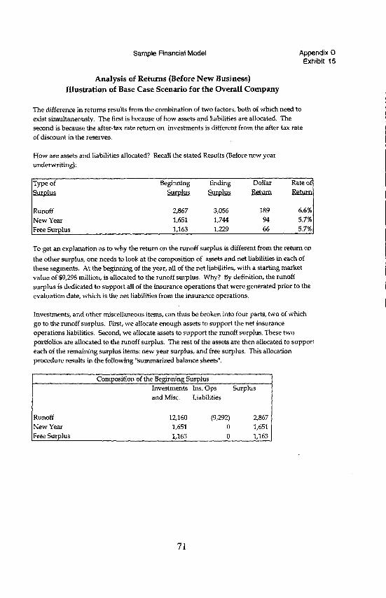
Sample Financial Model Appendix D Exhibit 15

Analysis of Returns (Before New Business) Illustration of Base Case Scenario for the Overall Company

The difference in returns results from the combination of two factors, both of which need to exist simultaneously. The first is because of how assets and liabilities are allocated. The second is because the after-tax rate return on investments is different from the after-tax rate of discount in the reserves.

How are assets and liabilities allocated? Recall the stated Results (Before new year

underwriting):

To get an explanation as to why the return on the runoff surplus is different from the return on

the other surplus, one needs to look at the composition of assets and net liabilities in each of

these segments. At the beginning of the year, all of the net liabilities, with a starting market value of $9,298 million, is allocated to the runoff surplus. Why? By definition, the runoff surplus is dedicated to support all of the insurance operations that were generated prior to the evaluation date, which is the net liabilities from the insurance operations.

Investments, and other miscellaneous items, can thus be broken into four parts, two of which go to the runoff surplus. First, we allocate enough assets to support the net insurance operations liabilities. Second, we allocate assets to support the runoff surplus. These two

portfolios are allocated to the runoff surplus. The rest of the assets are then allocated to supper! each of the remaining surplus items: new year surplus, and free surplus. This allocation procedure results in the following “summarized balance sheets”.

Composition of the Beginning Surplus

Investments Ins. Ops SUl-plUS

and Misc. Liabilities

Runoff 12,160 (9,292) 2,867 New Year 1,651 0 1,651 Free Surplus 1,163 0 1,163

71

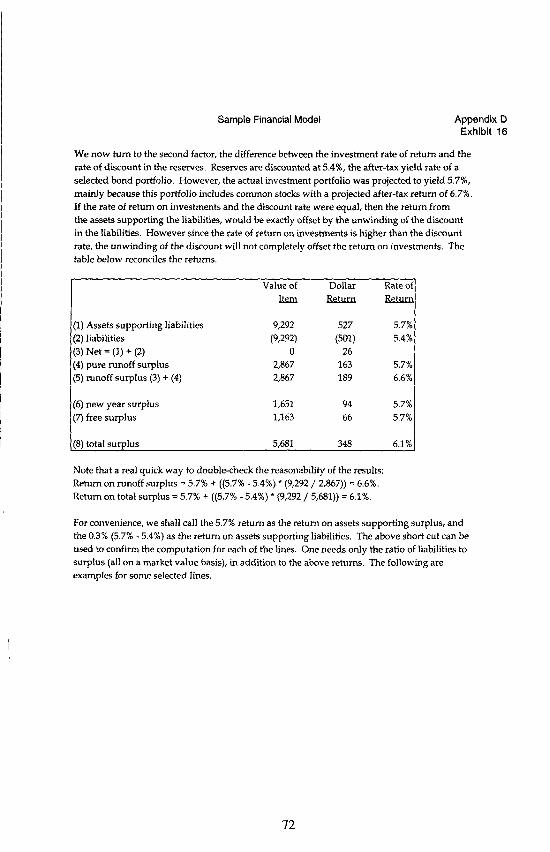
Sample Financial Model Appendix D Exhibit 16

We now turn to the second factor, the difference between the investment rate of return and the rate of discount in the reserves. Reserves are discounted at 5.4%, the after-tax yield rate of a

selected bond portfolio. However, the actual investment portfolio was projected to yield 5.7%, mainly because this portfolio includes common stocks with a projected after-tax return of 6.7%. If the rate of return on investments and the discount rate were equal, then the return from the assets supporting the liabilities, would be exactly offset by the unwinding of the discount in the liabilities. However since the rate of return on investments is higher than the discount

rate, the unwinding of the discount will not completely offset the return on investments. The table below reconciles the returns.

Value of Dollar Rate of

m !?%eum lL6sm.n

(1) Assets supporting liabilities 9,292 527 5.7%

(2) liabilities (9,292) (501) 5.4%

(3) Net = (1) + (2) 0 26

(4) pure runoff surplus 2,867 163 5.7%

(5) runoff surplus (3) + (4) 2,867 189 6.6%

(6) new year surplus

(7) free surplus

1,651 94 5.7% 1,163 66 5.7%

[(S) total surplus 5,681 348 6.l%j

Note that a real quick way to double-check the reasonability of the results: Return on runoff surplus = 5.7% + ((5.7% - 5.4%) * (9,292 / 2,867)) = 6.6%. Return on total surplus = 5.7% + ((5.7% - 5.4%) * (9,292 / 5,681)) = 6.1%.

For convenience, we shall call the 5.7% return as the return on assets supporting surplus, and

the 0.3% (5.7% - 5.4%) as the return on assets supporting liabilities. The above short cut can be used to confirm the computation for each of the lines. One needs only the ratio of liabilities to surplus (all on a market value basis), in addition to the above returns. The following are examples for some selected lines.

72

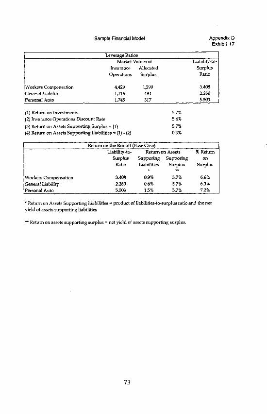
Sample Financial Model Appendix D Exhibit 17

Leverage Ratios Market Values of Liability-to-

Insurance

Operations

Workers Compensation 4,429 General Liability 1,116 Personal Auto 1,745

(1) Return on Investments (2) Insurance Operations Discount Rate

(3) Return on Assets Supporting Surplus = (1) (4) Return on Assets Supporting Liabilities = (1) - (2)

Allocated Surplus

1,299 494 317

5.7% 5.4%

5.7% 0.3%

Surplus Ratio

3.408 2.260 5.503

Return on the Runoff (Base Case) Liability-to- Return on Assets % Return

surp1us supporing supporing on Ratio Liabilities surplus Surplus

I *t

Workers Compensation 3.408 0.9% 5.7% 6.6%

General Liability 2.260 0.6% 5.7% 6.3%

Personal Auto 5.503 1.5% 5.7% 7.2%

* Return on Assets Supporting Liabilities = product of liabilities-to-surplus ratio and the net

yield of assets supporting liabilities

l * Return on assets supporting surplus = net yield of assets supporting surplus.

73

Sample Financial Model Appendix D Exhibit 18

Analysis of Change in Inflation and Interest Rates

Impact on the Rehnn on Runoff Surplus

In the illustrated alternative scenario, we assumed that both inflation and interest rates jump by 200 basis points and remain at the new level. The model assumes that the nominal paid

loss and adjustment expenses increase at the 2% annual rate. The only exception is that a

portion of workers camp indemnity reserves, in the non-COLA states, are not sensitive to chnages in inflation. All other expenses, except for acquisition expenses, grow at the rate of inflation. There are other consequences that are considered in the model.

First, the retrospective premiums are sensitive to loss experience, and should similarly

increase, but not necessarily at the same rate. The increase in premium is dependent on the retrospective contracts. In the illustrated scenario, the sensitivity of retro premium to loss

experience was based on the company’s historic premium sensitivity to loss and was heavily

dependent on the relative age at which the loss development occurs.

Second, one needs to consider the actual reaction of held reserves to the change in inflation

outlook. From a market value perspective, held reserves affect only the timing of

income taxes. Unfortunately, the reaction of held reserves to changes in inflation are not easily quantifiable. The difficulty stems not from theoretical reasons, since one can easily quantify

such impact, rather the difficulty is in attempting to mimic the real world. The standard actuarial techniques do not consider inflation implicitly. True, Inflation is explicitly projected

in the standard techniques, but these techniques average out inflation throughout the life of the policy or accident year and, as a result, do not calculate reserves under different inflation scenarios. In our scenario, WC nominal reserves ultimately grow 14% because of the 200 basis points jump in inflation. Company managers do not increase and reduce the reserve levels by

such levels just because inflation has gone up. Because of these considerations, the scenario above assumes that the nominal held reserves increase at the rate of inflation.

Third, All the changes above will impact future earned premium and incurred loss and

expenses. The tax implications from these earnings and losses are considered in the model.

The change of 200 basis points in interest rates causes a change of 130 basis points in the discount rate, since the discount rate is an after-tax rate.

We had discussed previously the impact on investments from a 200 basis points increase in interest rates. Overall, the after-tax return on investments drops from 5.7% in the base case scenario, to 0.8% in the alternative scenario.

74

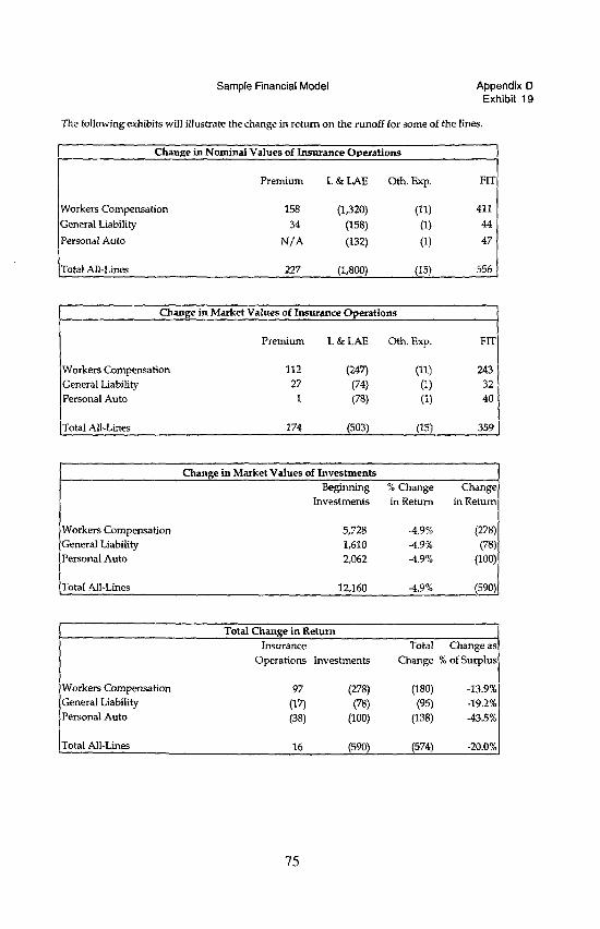
Sample Financial Model Appendix 0 Exhibit 19

The following exhibits will illustrate the change in return on the runoff for some of the lines.

Change in Nominal Values of Insurance Operations

Workers Compensation

General Liability

Personal Auto

Total All-Lines

Premium L&LAE 0th. Exp. FI-I

158 (1,320) (11) 411

34 (158) (1) 44

WA (132) (1) 47

227 (L8C’o) (15) 556

Change in Market Values of Insurance Operations

Premium L&LAE 0th. Exp.

Workers Compensation 112 (247) (11) General Liability 27 (74) (1) Personal Auto 1 (78) (1)

7

FlT

243 32 40

Total All-Lines 174 (503) (15) 359

Change in Market Values of Investments Beginning % Change Change

Investments in Return in Return

Workers Compensation 5,728 -4.9% (278) General Liability 1,610 -4.9% (78) Personal Auto 2,062 -4.9% W)

Total All-Lines 12,160 4.9% (59O)l

Total Change in Return

Insurance Operations Investments

Total Change as

Change % of Surplus

Workers Compensation General Liability Personal Auto

(278) UW -13.9%

(78) (95) -19.2%

(38) WJ) (138) -43.5%

Total All-Lines lb (590) (574) -20.0%

75

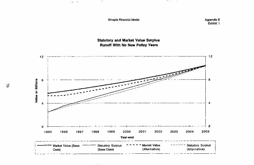
Smaple Financial Model Appendix E Exhibii 1

Statutory and Market Value Surplus Runoff With No New Policy Years

12 12

l 0-

1995 1996 1997 1998 1999 2000 2001 2002 2003

Year-end

i-o 2004 2005

Market Value (Base - Statutory Surplus - - - - - Market Value ---__---- Statutoty Surplus Case) (Base Case) (Alternative) (Alternative)

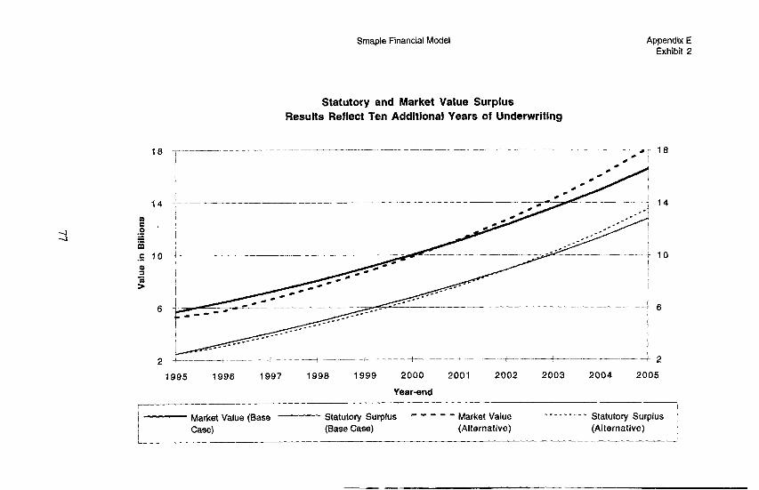
Smaple Financial Model Appendix E Exhibit 2

18

6

2

Statutory and Market Value Surplus Results Reflect Ten Additional Years of Underwriting

18

6

J- , .__ _/ ---.+ _ .-.A m.-bp-L .- .- ~cm---~-------:-.- 4 2

1995 1996 1997 1998 1999 2000 2001 2002 2003 2004 2005

Year-end

Market Value (Base ~ Statutoty Surplus -s--m Market Value --------- Statutory Surplus Case) (Base Case) (Alternative) (Alternative)

1 1 I

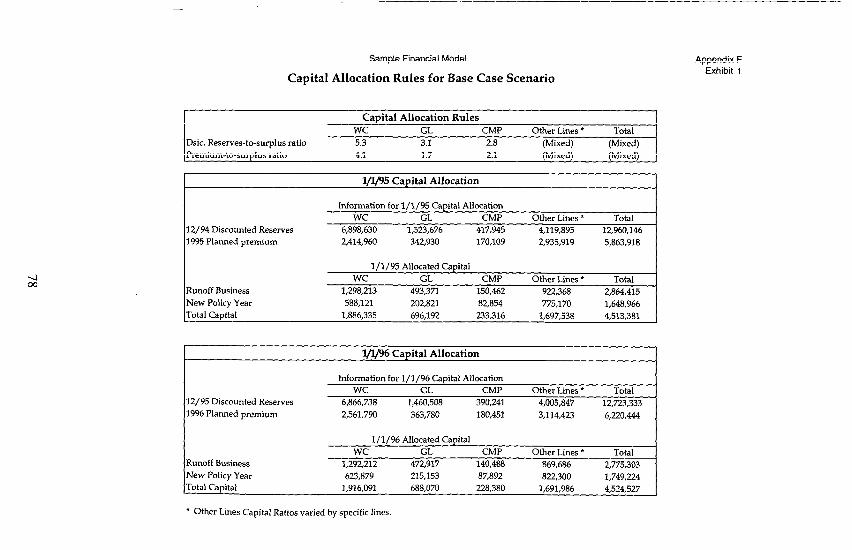
Sample Financial Model

Capital Allocation Rules for Base Case Scenario

Appendix F Exhibit 1

Dsic. Reserves-to-surplus ratio Premium-to-surplus ratio

Capital Allocation Rules WC GL CMP Other Lines * T&II 5.3 3.1 2.8 (Mixed) (Mixed) 4.1 1.7 2.1 (Mixed) (Mixed)

l/495 Capital Allocation

12/94 Discounted Reserves 1995 Planned premium

Information for l/1/95 Capital Allocation WC GL CMP

6,898,630 1523,676 417,945 2414,960 342,930 170,109

Other Lines * Total 4,119,895 12,960,146 2,935,919 5,863,918

Runoff Business New Policy Year Total Capital

l/1/95 Allocated Capital WC GL CMP Other Lines * Total

1,298,213 493,371 150,462 922,368 2,864,415 588,121 202,821 82,854 775,170 l&48,966

l&%,335 696,192 233,316 1,697,538 4,513,361

l/l/96 Capital Allocation

12/95 Discounted Reserves 1996 Planned premium

Information for l/1/96 Capital Allocation WC GL CMP

6,866,738 1,460,508 390,241 2,561,790 363,780 180,451

Other Lines l Total 4,005,547 12,723333 3,114,423 6,220,444

Runoff Business New Policy Year Total Capital

l/1/96 Allocated Capital WC GL CMP Other Lines * Total

1,292,212 472,917 140,488 869,686 2,775,303 623,879 215,153 87,892 522,300 1,749,224

1,9l6,091 688,070 228,380 1,691,986 4,524,527

l Other Lines Capital Ratios varied by specific lines.

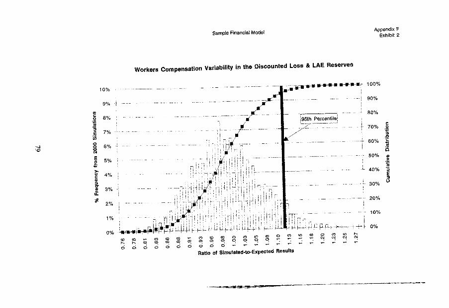
Sample Financial Model Appendix F Exhibit 2

10%

9%

Workers Compensation Variability in the Discounted LOSS & LAE Reserves

--

195th Percen$ e~-:~ -

/’

I

90%

80%

50%

Ratio of Simulated-to-Expected Results

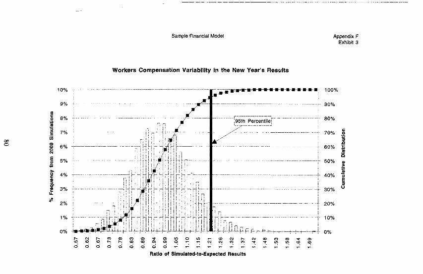
Sample Financial Model

Workers Compensation Variability in the New Year’s Results

4%

3%

2%

1%

0%

Appendix F Exhibit 3

Ratio of Simulated-to-Expected Results

1976

1977

1978 1979

1980 1981

1982

1983

1984

1985 1986 1987

1988

19989 1990

1991

1992

1993 1994

Impact of Medical Inflation Illustration based on a Fifteen-Year Triangle where Me Dollar amounts and the payment patterns are the Fixed Basis for Further Simulations

Appendix G Exhibit 1

Payments m Nommal Dollars ($M’ IlliOnS) 1 2 3 4 5 6 7 8 9 10 11 12 13 14 15

600 263 114 6.58 285 125 Tl3 311 138 778 346 153 864 383 171 956 427 186

1,067 46.5 197 1,161 493 no 1,233 524 226 1,311 564 240 1,409 601 256 1,502 640 276 -. 1,600 689 J 301 UC 327 1,878 817 351 2,042 877 372 2,193 929 389 /

50 22 10 4 55 24 11 5 61 27 12 5 68 30 13 5 74 32 13 6 79 34 14 6

90 38 16 7

131 56

2 1 0 0 0 0 2 1

I 0 0 0 0 TF

;

2 1 0 I- j

0 0 0 2 1 2

.g+

;-

0 ,-O O 0

-r- w 0 0 0 0

fi 0 :

; 0 0

,

1

,g,

_. ,~ 0-r-~ O ’

3 1 1 4 2 1

2,323 974 J 2,434 r -

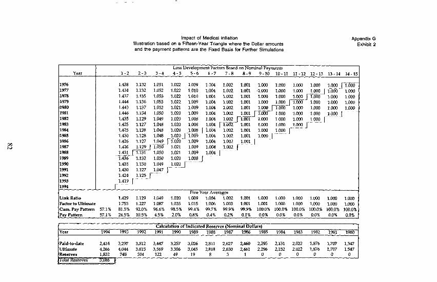
w

impact of Medical Inflation Illustration based on a Fifteen-Year Triangle where the Dollar amounts and the payment patterns are the Fixed Basis for Further Simulations

Appendix G Exhibit 2

Loss Development Factors Based on Nominal Payments 1-2 2-3 3-4 4-5 5-6 6-7 7-8 8-9 9-10 lo-11 11-12 12-13 13-14 14-15

-. 1.000 1.ooaa

1.cJMxM1.000 ix00 1.000

1.000 1.oou

1 1.000

1.000 1.000

1976 1.438 1.132 1.051 1.022 1.009 1.004 1.002 mn l.ooO l.O@l 1.000 1977 1.434 1.132 1.052 1.022 1.010 1.004 1.002 1.001 .l.Ooo 1.000 1.000 1978 1.437 1.135 1.053 1.022 1.010 1.004 1.002 1.001 l.OO+l 1.000 l.OOQ lY7Y

J 1.444 1.136 1.053 1.022 1.009 1.004 1.002 l.OOl l.OQO l.OOOJ-iXS 1.000

1980 1.443 1.137 1.052 1.021 1.009 l.OiM 1.002 1.001 l.COO 1.090 Loco 1.090 1981 1.446 1.134 1.050 1.020 l.CQP l.cQ4 1.000 l.OGU 1.000 1982 1.435 1.129 1.049 1.020 1.008 1.004 ::ztz ,risz l.ooO 1.000 l.ooO 1983 1.425 1.127 1.048 1.020 1.008 1.004 rmC

J 1.001 1.000 1.000 1.000 J

1984 1.425 1.128 1.048 1.020 l.oof3of3?xi4 1.002 l.cOl l.OGO 1.000 r 1985 1.430 1.128 1.048 1.020 pc9 1.004 1.002 1.001 l.M)o 1986 1.426 1.127 1.049 1.002 l.Dol 1987 1.426 1.129 1

r1.020 1.009 1.004 I ~-- 1.050 1.021 1.009 1.004 1.002 r- --

1988 1.431 _1- 1.050 1.021 1.009 1.004 --

J 1P89 1.436 1.132 1.050 1.020 1.008 1 1990 1.435 1.130 1.049 1991 1.430 1.127 1.047 [

l.O2O_J-

1992 1.424 1.125J 1993 1.419 r 1994 r-

Five Year Averages Link Ratio 1.429 1.129 1.049 1.020 1.009 1.004 1.002 1.001 1.000 1.000 1.000 Loo0 1.000 LOCO Factor to Ultimate 1.753 I.227 1.087 1.035 1.015 1.006 1.003 1.001 1.001 1.000 1.ooo l.Doo 1.000 l.ooO Cum. Pay Pattern 57.1% 81.5% 92.0% 96.6% 98.5% 99.4% 99.7% 99.9% 99.9% 100.0% 100.0% lM).O% 100.0% 100.0% 100.0% Pay Pattern 57.1% 24.5% 10.5% 4.5% 2.0% 0.8% 0.4% 0.2% 0.1% 0.0% 0.0% 0.0% 0.0% 0.0% 0.0%

1.000 1.000

rJEJ --

i

Y-28.X 1994 Calculation of indicated Reserves (Nominal Dollars)

1993 1992 1991 1990 1989 1988 1987 1986 1985 1984 1983 1982 1981 1980

Paid-to-date 2,434 3,297 3,512 3,447 3,257 3,026 2,811 2,627 2,460 2,295 2,151 2,022 1,876 1,707 1,547 Ultimate 4,266 4,044 3,815 3,569 3,306 3,045 2,818 2,630 2,461 2,296 2,152 2,022 1,876 1,707 1,547 Reserves 1.832 748 304 122 49 19 8 3 1 0 0 0 0 0 0 I

otal Keserves 3,LKlb I

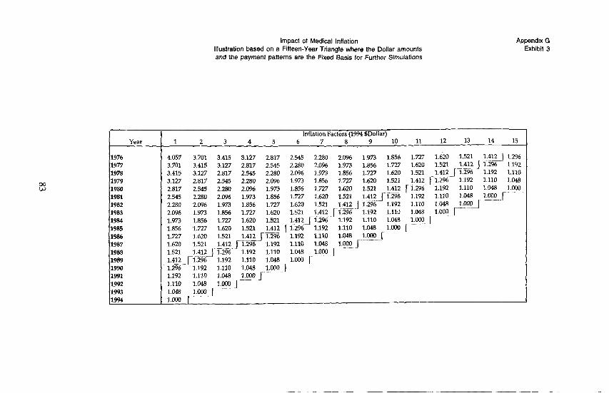
1976 1977 1978 1979 1980 1981 1982 1983 1984 1985 1986 1987 1988 1989 1990 1991 1992 1993 1994

Impact of Medical Inflation Illustration based on a Fifteen-Year Triangle where the Dollar amounts and the payment patterns are the Fixed Basis for Further Simulations

Appendix G Exhibit 3

Inflation Factors (19% $Dollar) 1 2 3 4 5 6 7 8 9 10 11 12 13 14 15

4.057 3.701 3.701 3.415 3.415 3.127 3.127 2.817 2.817 2.545 2.545 2.280 2.280 2.096 2.096 1.973 1.973 1.856 1.856 1.727 1.727 1.620 1.620 1.521 1.521 1.412 1.4giis- 1.296 1.192 1.192 1.110 1.110 1.048

3.415 3.127 2.817 2.545 2.280 2.096 3.127 2.817 2.545 2.280 2.096 1.973 2.817 2.545 2.280 2.096 1.973 1.854 2.545 2.280 2.094 1.973 1.856 1.727 2.280 2.096 1.973 1.856 1.727 1.620 2.096 1.973 1.856 1.727 1.620 1.521 1.973 1.856 1.727 1.620 1.521 1.412 1.856 1.727 1.620 1.521 1.412 1.296 ~_~

I.4121 1.2% 1

1.727 1.620 1.521 1.192 1.620 1.521 1.412 1 1.2% 1.192 1.110

1.973 1.856 1.727 1.620 1.521 1.412

1 1.29a ' 1.192

1.110 1.048

1.192 1.110 1.048 1.oQo 1.296 1.192 1.110 1.048 1.E~ J

1.048 1.000 r 1.192 1.110 1.048 l.OaO J 1.110 I.048 1.000 r I.048 l.m 1

1.856 1.727 1.620 1.727 1.620 1.521 1.620 1.521 1.412 1.521 1.412Jx296m

,$A!; I ;:;z ;:;z

1.110 1.048 1.048 1.@30

- 1.192 1.110 1.048 l.ooo

I ~-~

1.521 1.412 j 1.296 1.412 j 1.296 1.192

I i.296 ~- 1.192 1.110 1.048 1.192

1.110 1.048

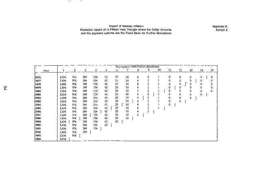
I

Year

t- 1976

Impact of Medical Inflation Illustration based on a Fifteen-Year Triangle where the Dollar amounts and the payment patterns are the Fixed Basis for Further Simulations

Appendix G Exhibit 4

Payments in 1994 Dollars (5millions) 1 2 3 4 5 6 7 8 9 10 11 12 13 14 15

2,434 974 389 156 62 2s 10 4 2 1 0 0 ’ 2,434 974 389 156 62 25 10 4 2 1 0 0 i I : i 21434 974 389 156 62 25 10 4 2 1 0 ro 2,434 974 389 156 62 25 10 4 2

2,434 974 389 156 62 25 10 4 :

: I

E,; ; i ;

2,434 974 389 156 62 25 10 2,434 974 389 156 62 25 10 i I

I ; ;

; 0 0 I

0 2,434 974 389 156 62 25 10 1 4 1 2,434 974 389 156 62 25110 4 2 2,434 974 389 156 62 1 ~25 10 4 2,434 974 389 156 1 62 25 10 2.434 974 389 1 156 62 25 2,434 974 1 389 156 62 25 2,434 1 974 389 156 2,434 974 389 156 2,434 974 389 156

1 1

2,434 974 389 2,434 974 2,434 1

)

Year

1976 1977

)I978 1979 1980

1981

1982 1983

1984

1985 1986

1987 1988 1989

1990 1991

1992 1993

1994

Link Ratio

impact of Medical Inflation Appendix G Illustration based on a Fifteen-Year Triangle where the Dollar amounts Exhibit 5

Loss Development Factors Based on Payments Converted to 1994 $Dollars 1-2 2-3 3-4 4-5 5-6 6-7 7-8 8-9 9-10 lo-11 11-12 12-13 13-14 14-l:

1.006 1.002 1.001 1.ooo 1.000 l.ooil 1.000 l.ooO 1.000 1 1.m 1.006 1.002 1.001 1.000 l.ooo 1.000 l.Oca l.OOo] 1.000 1.000 1.006 1.002 1 .I01 l.oco l.ooo l.M)O 1.000 f 1.000 mail 1.000 1.006 1.002 1.001 1.000 1.000 1.000 pl.004 l.m 1.000 l.OiXJ

1.000 1.000

1.400 1.114 1.041 1.016 1.404 I.114 1.u41 1.016 1.400 1.114 1.041 1.016 1.400 1.114 1.041 1.016 1.4w 1.114 1.041 1.016 I.400 1.114 1.041 1.016 1.400 1.114 1.041 1.016 1.m 1.114 1.041 1.016 1.400 1.114 1.041 1.016 1.400 1.114 1.041 1.016 1.400 1.114 1.041 J 1.016 1.400 1.114 p.041 1.016 I .4ooJiXT 1.041 1.016 1.400 1.114 1.041 1.016 1.4&I 1.114 1.041 1.016 1.400 1.114 1.041 r

_-- _- 1.@96 1.002 1.001 looa 1.000 [ l.m 1.000 1.006 1.002 1.001 1.000p1.mo l.oOa l.Ooa 1.006 1.002 1.001 p0 1.ooo 1.000 1.000 1.006 1.002J 1.001 l.ooO 1 .I00 1.ooo 1.000 1.m

-- 1.001

_fl.O06 l.ooo l.om 1.000 J

1.002 1.001 l.!?QO l.ooOJ 1.006 1.002 1.001 1.000 r 1.006 1.007. 1BOl~

1.000 1.000 l.C@l

I--

and the payment patterns are the Fixed Basis for Further Simulations

1.400 l.lM~j -- - ’

I- 1.400 r

Five Year Averages 1.400 1.114 1.041 1.016 1.@36 1.002 1.001 1.000 l.ooo l.OOO 1.000 l.ooo 1.000 l.M?O

Factor to Ultimate 1.667 1.190 1.068 1.026 1.010 1.004 I.002 1.001 l.UUU 1 .mJu 1.ooo l.KKl I.000 1.004 Cum.PayPa&m 60.0% 84.0% 93.6% 97.4% 99.0% 99.6% 99.8% 99.9% lM).O% 100.0% 100.0% 100.0% 100.0% 100.0% 100.0%

Pay Pattern 60.0% 24.0% 9.6% 3.8% 1.5% 0.6% 0.2% 0.1% 0.0% 0.0% 0.0% 0.0% 0.0% 0.0% 0.0%

Calculation of Indicated Reserves (in 1994 Ddlars) Y.SU 1994 1993 1992 1991 1990 1989 1988 1987 1986 1985 1984 1983 1982 1981 1980

Paid-to-date 2,434 3,408 3,797 3,953 4,015 4.040 4,050 4,054 4,056 4,056 4,057 4,057 4,057 4,057 4,057 Ultimate 4,057 4,057 4,057 4,057 4,057 4,057 4,057 4,057 4,057 4,057 4,057 4,057 4,a57 4,057 4,057 Reserves 1,623 649 260 104 42 17 7 3 1 0 0 0 0 0 0

‘otal Kesen’es L./U4 1

Impact of Medical Inflation Illustration based on a Fifteen-Year Triangle where the Dollar amounts and the payment patterns are the Fixed Basis for Further Simulations

Appendix G Exhibit 6

f Expected Payment of Reserves in XkaE r.Qhl199514e6mlspB19sszMM~zLMzzMz;izM14zap5zMM~~

1994 Dollars 2,704 1.623 649 260 104 42 17 7 3 1 0 0 0 0 0

Reinflated Payments 4% InfIation 2,890 1,688 702 292 121 51 21 9 4 2 1 0 0 0 0 8% InfIation 3,085 1,752 757 327 141 61 26 11 5 2 1 0 0 0 0 10% Inflation 3,187 1,765 7135 346 152 67 29 13 6 3 1 0 0 0 0

PC?,iOd 1970 Dot 1971 Dot 1972 oec

12-a

Appendix H Exhibit 1 Page 1

DeYe,opment Faclors 1c.r lndcmnlty an* Audi 24 .36 36-48 48.60 60-72 72.64 84.96 96.106 106. 120 120. 132 132.144

1.055 1.040 1.026 1.021 1.016 1.016 1012 1.094 1.055 1.041 1.026 1.024 1016 1.011 1.010

1.168 1.093 I.065 1.043 1.Q32 1.025 1.016 1.018 1.018 1973Dcc ,974 ooc 2.334 ,976 0% 2.310 ,976 ooc 2.262 ,977 oec 2.192

1978 DE 2.246 1979Dec 2.199 1980 oec 2.169 1981 oec 2.19, 1982 oec 2.179

1.386 1.159 1.096 1.062 1.385 1.164 1.093 l.obB 1.398 1.190 1.116 1.076 1.388 1.195 1.117 1,069 1.046 1.031 1.027 1.020 1.017 1.013 1.397 1.191 1.111 1.070 1.048 1.031 1.023 1.019 1.016 1.015 1.407 1.193 1.113 1.068 Is!48 1.031 1.027 1.022 1.019 1.016 1.409 1.192 1.109 I.068 1.046 1.036 1.027 1.023 1.020 1.019 I.400 1.209 1.107 1.074 1.060 1.038 I.030 1.023 1.020 1.017 I.400 I.185 1.115 1.075 1.056 1.041 1.032 1.025 1.019 1.017 1.395 1.207 1.131 1.098 1.059 1.046 I.043 1.026 1.024 1.020

1.049 1.033 1.025 1.020 1.017 1.012 I.044 1.034 1.022 1.019 1.016 1.013 1.051 1.037 1.026 1.021 1.016 f.013

1983 oec 2.263 1.437 1.227 1.140 1.066 1.064 1.046 1.037 1.025 1.022 1.017 1984 Dee 2.345 1.473 1.228 1.134 1.089 1.004 1.044 1.033 1.027 1.018 1985 Dee 2.422 1.473 1.245 1.140 1 .ow 1.057 1.041 I.030 1.020

2 1986 0% 2.377 I.500 1.237 1.133 1.065 1.055 1.038 1.026

1987 Dee 2.452 1.496 1234 1.127 t.oao 1.053 1.034 1966DSC 2.496 1.496 1.226 1.126 1.074 1.047 ,889Dec 2.502 1.612 1.231 1.121 1.068 1990 O%C 2.666 1.520 1.232 1.109 1991 oec 2.529 1.607 1.21, 1992 Ilee 2.464 1.470 1993Dec 2.426

i994 Dee

1 2 3 4 5 6 7 6 9 10 II

Lc,g”omlal PalameferS:+ ll7" Ok 9.82 -1.56 .2.16 -2.62 -3.00 -3.33 .3.69 -3.88 -4.03 -4.21

sigma 0.101934 0.113606 0.124266 0.132060 O.i54326 0.12574l 0.167132 0.182388 0.167487 0.174078 0.203765

Simulated ATA" 2.304 I.364 1.167 1.136 1.063 I.059 1.039 1.019 1.021 1.014 l.Ot6

* ~ognormal parametersare bated on lilting B logno~aldisltibulionlo the column olage.to-age fackxs. To get a better 111,1he disidbulion is citto(ATA. I), ralherthan(olhe ag~~~agelaclors Wemselves. a* the ~mukledage-lo-age kr,btS We USedin B Mo~~wZMIO simulalion.and arederived by invrd,ng the C~m~latiw Density of ~h~lognormal,a~umingno correb#on among 6% &vwiopmentsi dillerentmalurities.

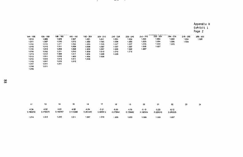
Appendix H Exhibit 1 Page 2

228.240 1.006 1 .c‘% 1.007 I.007 I.006

1.010

240-252 1 .xX 1 .xX 1.006 1.045 1.007

252.264 1.044 1.004 1.006 1 .I07

264-276 1.004 1.006 ma

276.268 1.004 1.005

286 .m 1 .w5

(44.156

1.013 1.011 I.010 I.013

156-166

1.009 1 .W? 1.012 1.012

168-160

1.008 1.010 I.011 1.01,

1.010 1.013 I.009 1.014 1.012 1.01, 1.013 1.012 1 ma 1.013 I.011 1.010 ,.0,4 I.012 1.012 1.013 I.011 1.012 1.017 1.011 t.01, 1.016 1.011

1.015

,ao- 192 1.007 1.012 1 .wa l.cca 1.008 1.010 1.0,1 I.009 1.01, 1.012

192.204 204.216 216-228 1.021 i.Wl 1.004

1.w9 1.008

1.005 1 .x6 i.wa 1.007

~.coa I.007 1.007 1.009 I.007 1.006 1.009 ,.o,o 1.010 I.009 1 .w9 t .w9 I .309 1009 ~.MM

12 13 14 IS 16 17 16 IS 20 21 22 23 24

-4.34 -4.52 4.61 .4.65 4.64 -5.2, wx -4.95 4.19 -5.23 eJ.12 0.163310 0.176673 0.,60767 0.170093 0.291440 0.965613 0.279641 0 226962 0.190354 0.226015 0.280225

1.01. 1.013 I.010 1.011 1.007 1.016 l-006 1.w5 ,.W6 1.005 ,.oo7