the finance uncertainty multiplier

The Finance Uncertainty Multiplier∗

Iván Alfaro† Nicholas Bloom‡ Xiaoji Lin§

December 29, 2017

Abstract

We show how real and financial frictions amplify the impact of uncertainty shocks. Westart by building a model with real frictions, and show how adding financial frictions roughlydoubles the negative impact of uncertainty shocks. The reason is higher uncertainty alongsidefinancial frictions induces the standard negative real-options effects on the demand forcapital and labor, but also leads firms to hoard cash against future shocks, further reducinginvestment and hiring. We then test the model using a panel of US firms and a novelinstrumentation strategy for uncertainty exploiting differential firm exposure to exchangerate and factor price volatility. Consistent with the model we find that higher uncertaintyreduces firms’ investment, hiring, while increasing their cash holdings and cutting theirdividend payouts, particularly for financially constrained firms. This highlights why inperiods with greater financial frictions —like during the global-financial-crisis —uncertaintycan be particularly damaging.

JEL classification: D22, E23, E44, G32Keywords: Uncertainty, Financial frictions, Investment, Employment, Cash holding, Equitypayouts

∗We would like to thank our formal discussants Nicolas Crouzet, Ian Dew-Becker, Simon Gilchrist, Po-HsuanHsu, Gill Segal, Toni Whited, and the seminar audiences at the AEA, AFA, Beijing University, CEIBS, EconometricSociety, European Finance Association, Macro Finance Society Workshop, Melbourne Institute MacroeconomicPolicy Meetings, Midwest Finance Association, Minneapolis Fed, NY Fed, Stanford SITE, The Ohio StateUniversity, UBC Summer Finance Conference, University College London, University of North Carolina at ChapelHill, University of St. Andrews, University of Texas at Austin, University of Texas at Dallas, University of Toronto,Utah Winter Finance Conference, World Congress. The NSF and Alfred Sloan Foundation kindly provided researchsupport.†Department of Finance, BI Norwegian Business School, Nydalsveien 37, N-0484 Oslo, Norway. e-mail:

[email protected]‡Economics Department, Stanford University, 579 Serra Mall, Stanford CA 94305, email:[email protected]§Department of Finance, Fisher College of Business, The Ohio State University, 2100 Neil Avenue, Columbus

OH 43210. e-mail:[email protected]

1

1 Introduction

This paper seeks to address two related questions. First, why are uncertainty shocks in some

periods - like the 2007-2009 global financial crisis - associated with large drops in output, while

in other periods - like the Brexit vote or Trump election - are accompanied by steady economic

growth? Second, as Stock and Watson [2012] noted, uncertainty shocks and financial shocks are

highly correlated. Are these the same shock, or are they distinct shocks with an interrelated

impact, in which uncertainty is amplified by financial frictions?

To address these questions we build a heterogeneous firms dynamic model with two key

extensions. First, real and financial frictions: on the real side investment incurs fixed cost1,

and on the financing side issuing equity involves a fixed cost2. Second, uncertainty and financing

costs are both stochastic, with large temporary shocks. The model is calibrated, solved and then

simulated as a panel of heterogeneous firms.

We show two key results. Our first key result is a finance uncertainty multiplier (hereafter

FUM). Namely, adding financial frictions to the classical model of stochastic-volatility uncertainty

shocks - as in Dixit and Pindyck [1994], Abel and Eberly [1996] or Bloom [2009] - roughly

doubles the negative impact of uncertainty shocks on investment and hiring. In our simulation

an uncertainty shock with real and financial frictions leads to a peak drop in output of 2.4%, but

with only real frictions a drop of 1.3%. In a slightly abusive notation, where Y is output, σ is

uncertainty, and FC is financial adjustment costs, FUM = d2YdσdFC

≈ −2, i.e., introducing financial

costs roughly doubles the impact of uncertainty shocks on output.

Our second key result is that uncertainty shocks and financial shocks have an almost additive

impact on output. In our simulations, uncertainty shocks or financial shocks in models with real

and financial frictions each individually reduce output by 2.4%, but jointly reduce output by 4%.

We summarize these two results below in table 1. This reports the peak drop in aggregate

output in our calibrated model with only real frictions and an uncertainty shock is 1.3% (top left

1For example, Bertola and Caballero [1990], Davis and Haltiwanger [1992], Dixit and Pindyck [1994], Caballeroet al. [1995], Abel and Eberly [1996], or Cooper and Haltiwanger [2006].

2See, for example, Gomes [2001], Hennessy and Whited [2005], Hennessy and Whited [2007], Bolton et al. [2013],etc.

2

box). Adding financial frictions almost doubles the size of this drop to 2.4% (bottom left box).

Finally, adding a financial shock increases the impact by another two-thirds, yielding a drop in

output of 4.0% (bottom right). So collectively going from the classic uncertainty model to one

with financial frictions and simultaneous financial shocks roughly triples the impact of uncertainty

shocks, and can help explain why uncertainty shocks during periods like 2007-2009 were associated

with large drops in output.

Table 1Key results in simulation

Uncertainty Uncertainty

shock + financial shocks

Real frictions 1.3% n/a

Real+financial frictions 2.4% 4.0%

Notes: Results based on simulations of 30,000 firms of 1000-quarter length in the calibrated model (seesection 3.4.1). Going from top to bottom row shows adding financial frictions roughly doubles the impactof uncertainty shocks (a FUM is around 2). Going from the left to right column shows the additiveimpact of uncertainty shocks and financial shocks in models with both real and financial frictions.

Alongside the negative impact of uncertainty and finance shocks on investment and

employment, the model also predicts these shocks will lead firms to accumulate cash and reduce

equity payouts, as higher uncertainty causes firms to take a more cautious financial position. As

Figure 1 shows this is consistent with macro-data. It plots the quarterly VIX index - a common

proxy for uncertainty - alongside aggregate real and financial variables. The top two panels show

that times of high uncertainty (VIX) are associated with periods of low investment and employment

growth. The middle two panels shows that cash holding is positively associated with the VIX,

while dividend payout and equity repurchase are negatively related to the VIX. The bottom panels

also considers debt - which we model in an extension of our baseline model - and shows that the

total debt (the sum of the short-term and long-term debt) growth and the term structure of the

debt growth (short-term debt growth to long-term debt growth ratio) are both negatively related

with the VIX, implying firms cut debt (and particularly short-term debt) when uncertainty is

high.

The additional complexity in the model required to model: (a) real and financial frictions, and

3

(b) uncertainty and financial shocks, required us to make some simplifying assumptions. First,

we ignore labor adjustment costs - including these would likely increase the impact of uncertainty

shocks, since labor accounts for 2/3 of the cost share in our model. Second, we ignore general

equilibrium (GE) effects - including these would likely reduce the impact of uncertainty shocks

by allowing for offsetting price effects. As a partial response to this we also run a pseudo-GE

robustness test where we allow real wages and interest rates to move after uncertainty shocks

following typical changes observed in the data, and find our results are about 1/3 smaller but

qualitatively similar.3 Finally, we ignore debt financing (only allowing for equity financing), since

this would dramatically increase the complexity of the financial modeling (but with probably

limited impact on the real-side of the model). In an extension with debt rather than equity we

show uncertainty shocks generate similar results.

The second part of the paper tests this model using a micro-data panel of US firms with

measures of uncertainty, investment, employment, cash, debt and equity payments. To address

obvious concerns over endogeneity of uncertainty4 we employ a novel instrumentation strategy

for uncertainty exploiting differential firm exposure to exchange rate, factor price and policy

uncertainty. This identification strategy works well delivering a strong first-stage F-statistics and

passing Hansen over-identification tests. We find that higher uncertainty significantly reduces

investment (in tangible and intangible capital) and hiring, while also leading firms to more

cautiously manage their financial polices by increasing cash holdings and cutting debt, dividends

and stock-buy backs, consistent with the model (and macro data).

Our paper relates to three main literatures. First, the large uncertainty literature studying the

impact of heightened uncertainty and volatility on investment and employment.5 We build on the

3One reason is that wages and real interest rates do not move substantially over the cycle (e.g. King and Rebelo[1999]), and second increased uncertainty widens the Ss bands so that the economy is less responsive to pricechanges (e.g. Bloom et al. [2016]).

4See, for example, Nieuwerburgh and Veldkamp [2006], Bachmann and Moscarini [2012], Pastor and Veronesi[2012], Orlik and Veldkamp [2015], Berger et al. [2016], and Falgelbaum et al. [2016], for models and empirics onreverse causality with uncertainty and growth.

5Classic papers on uncertainty and growth included Bernanke [1983], Romer [1990], Ramey and Ramey [1995],Leahy and Whited [1996], Guiso and Parigi [1999], Bloom [2009], Bachmann and Bayer [2013], Fernandez-Villaverdeet al. [2011], Fernandez-Villaverde et al. [2015], and Christiano et al. [2014]. Several other papers look at uncertaintyshocks - for example, Bansal and Yaron [2004] and Segal et al. [2015] look at the consumption and financialimplications of uncertainty, Handley and Limao [2012] at uncertainty and trade, Ilut and Schneider [2014] modelambiguity aversion as an alternative to stochastic volatility, and Basu and Bundick [2017] examine uncertainty

4

literature to show the joint importance of real and financial frictions for investment, hiring and

financial dynamics, and importantly how adding financial shocks can roughly double the impact

of uncertainty shocks.

Second, the literature on financial frictions and business cycles6. We build on this literature

to argue it is not a choice between uncertainty shocks and financial shocks as to which drives

recessions, but instead these shocks amplify each other so they cannot be considered individually.

Finally, the finance literature that studies the determinants of corporate financing choices.7 We

are complementary to these studies by showing that uncertainty shocks have significant impact

on firms real and financial flows, examined in both calibrated macro models and well identified

micro-data estimations.

The rest of the paper is laid out as follows. In section 2 we write down the model. In section 3

we present the main quantitative results of the model. In section 4 we describe the instrumentation

strategy and international data that we use in the paper. In section 5 we present the empirical

findings on the effects of uncertainty shocks on both real and financial activity of firms. Section 6

concludes.

2 Model

The model features a continuum of heterogeneous firms facing uncertainty shocks and financial

frictions. Furthermore, financial adjustment costs vary over time and across firms. Firms choose

optimal levels of physical capital investment, labor, and cash holding each period to maximize the

market value of equity.

shocks in a sticky-price Keynesian model, and Berger et al. [2016] on news vs uncertainty. A related literature ondisaster shocks - for example, Rietz [1988], Barro [2006], and Gourio [2012] - is also connected to this paper, inthat disasters can be interpreted as periods of combined uncertainty and financial shocks, and indeed can lead touncertainty through belief updating (e.g. Orlik and Veldkamp [2015]).

6For example, Alessandri and Mumtaz [2016] and Lhuissier and Tripier [2016] show in VAR estimates a stronginteraction effect of financial constraints on uncertainty. More generally, Jermann and Quadrini [2012], Christianoet al. [2014], and Gilchrist et al. [2014], Arellano et al. [2016], show that financial frictions are important to explainthe aggregate fluctuations for the recent financial crisis.

7For example, Rajan and Zingales [1995], Welch [2004], Moyen [2004], Hennessy and Whited [2005], Riddick andWhited [2009], DeAngelo et al. [2011], Bolton et al. [2011], Rampini and Viswanathan [2013], Chen et al. [2014],and Chen [2016] study the impact of various frictions on firms’financing policies, including equity, debt, liquiditymanagement, etc.

5

2.1 Technology

Firms use physical capital (Kt) and labor (Lt) to produce a homogeneous good (Yt). To save on

notation, we omit the firm index whenever possible. The production function is Cobb-Douglas,

given by

Yt = ZtKαt L

1−αt , (1)

in which Zt is firms’productivity. The firm faces an isoelastic demand curve with elasticity (ε),

Qt = BP−εt ,

where B is a demand shifter. These can be combined into a revenue function R (Zt, B,Kt, Lt) =

Z1−1/εt B1/εK

α(1−1/ε)t (Lt)

(1−α)(1−1/ε) . For analytical tractability we define a = α (1− 1/ε) and

b = (1− α) (1− 1/ε) , and substitute Z1−a−bt = Z1−1/εt X1/ε. With these redefinitions we have

S (Zt, Kt, Lt) = Z1−a−bt Kat L

bt .

Wages are normalized to 1 denoted as W . Given employment is flexible, we can obtain optimal

labor.8 Note that labor can be pre-optimized out even with financial frictions which will be

discussed later.

Productivity is defined as a firm-specific productivity process, following an AR(1) process

zt+1 = ρzzt + σtεzt+1

in which zt+1 = log(Zt+1), εzt+1 is an i.i.d. standard normal shock (drawn independently across

firms), and ρz, and σt are the autocorrelation and conditional volatility of the productivity process.

The firm stochastic volatility process is assumed for simplicity to follow a two-point Markov

chains

σt ∈ {σL, σH} ,where Pr (σt+1 = σj|σt = σk) = πσk,j. (2)

8Pre-optimized labor is given by(bWZ1−a−bt Ka

t

) 11−b .

6

Physical capital accumulation is given by

Kt+1 = (1− δ)Kt + It, (3)

where It represents investment and δ denotes the capital depreciation rate.

We assume that capital investment entails nonconvex adjustment costs, denoted as Gt, which

are given by:

Gt = ckSt1{It 6=0}, (4)

in which ck > 0 is constant. The capital adjustment costs include planning and installation costs,

learning to use the new equipment, or the fact that production is temporarily interrupted. The

nonconvex costs ckSt1{It 6=0} capture the costs of adjusting capital that are independent of the size

of the investment.

We also assume that there is a fixed production cost F ≥ 0. Firms need to pay this cost

regardless of investment and hiring decisions every period. Hence firms’operating profit (Πt) is

revenue minus wages and fixed cost of production, given by

Πt = St − WLt − F. (5)

2.2 Cash holding

Firms save in cash (Nt+1) which represents the liquid asset that firms hold. Cash accumulation

evolves according to the process

Nt+1 = (1 + rn)Nt +Ht, (6)

where Ht is the investment in cash and rn > 0 is the return on holding cash. Following Cooley

and Quadrini [2001] and Hennessy et al. [2007], we assume that return on cash is strictly less

than the risk free rate rf (i.e., rn < rf). This assumption is consistent with Graham [2000] who

documents that the tax rates on cash retentions generally exceed tax rates on interest income for

7

bondholders, making cash holding tax-disadvantaged. Lastly, cash is freely adjusted.

2.3 External financing costs

When the sum of investment in capital, investment adjustment cost and investment in cash exceeds

the operating profit, firms can take external funds by issuing equity. External equity financing

is costly for firms. The financing costs include both direct costs (for example, flotation costs

- underwriting, legal and registration fees), and indirect (unobserved) costs due to asymmetric

information and managerial incentive problems, among others.9

Because equity financing costs will be paid only if payouts are negative, we define the firm’s

payout before financing cost (Et) as operating profit minus investment in capital and cash

accumulation, less investment adjustment costs

Et = Πt − It −Ht −Gt. (7)

Furthermore, external equity financing costs vary over time and across firms.10 The micro-

foundations of time-varying financing conditions include endogenous time-varying adverse selection

problems in Eisfeldt [2004], Kurlat [2013], and Bigio [2015] who show that uncertainty increases

the adverse selection cost from equity offerings (raising financing costs), agency frictions varying

over time as in Bernanke and Gertler [1989] and Carlstrom and Fuerst [1997], and time-varying

liquidity as in Pastor and Stambaugh [2003]. Furthermore, empirically, Choe et al. [1993] find that

the adverse selection costs measured as negative price reaction to SEO announcement is higher

in contractions and lower in expansions, suggesting changes in information symmetries between

firms and investors are likely to vary over time. Lee and Masulis [2009] show that seasoned equity

issuance costs are higher with poor accounting information.

9These costs are estimated to be substantial. For example, Altinkilic and Hansen [2000] estimate theunderwriting fee ranging from 4.37% to 6.32% of the capital raised in their sample. In addition, a few empiricalpapers also seek to establish the importance of the indirect costs of equity issuance. Asquith and Mullins [1986]find that the announcement of equity offerings reduces stock prices on average by −3% and this price reduction asa fraction of the new equity issue is on average −31%.10Erel et al. [2012] show that firms’ access to external finance markets also changes with macroeconomic

conditions. Kahle and Stulz [2013] find that net equity issuance falls more substantially than debt issuance duringthe recent financial crisis suggesting that shocks to the corporate credit supply are not likely to be the cause forthe reduction in firms’capital expenditures in 2007-2008.

8

As such, we use ηt to capture the time-varying financing conditions that also vary across firms;

it is assumed for simplicity to follow a two-point Markov chain

ηt ∈ {ηL, ηH} ,where Pr(ηt+1 = ηj|ηt = ηk

)= πηk,j. (8)

We do not explicitly model the sources of the equity financing costs. Rather, we attempt to

capture the effect of the costs in a reduced-form fashion as in Gomes [2001]. The external equity

costs Ψt are assumed to scale with firm size as measured by the revenue:

Ψt = φ (ηt, σt)St1{Et<0}. (9)

Finally, firms do not incur costs when paying dividends or repurchasing shares. Note that

φ (ηt, σt) captures the marginal cost of external financing which affects both optimal investment

and cash holding policies, similar to Eisfeldt and Muir [2016] who model a time-varying financing

condition by an AR(1) process.

Finally, note that the marginal external equity financing cost depends on both time-varying

financing condition ηt and time-varying uncertainty σt. This assumption captures the fact that

periods of high costs of external financing are associated with heightened uncertainty. For example,

the aggregate Baa-Aaa spread on corporate bonds has a correlation with the VIX at around 0.65.

As such, we assume φ (ηt, σt) = ηt + λ with λ > 0 when σt = σH , and φ (ηt, σt) = ηt when when

σt = σL, to capture the positive correlation between financing cost and uncertainty in the data.

2.4 Firm’s problem

Firms solve the maximization problem by choosing capital investment, labor, and cash holding

optimally:

Vt = maxIt,Lt,Kt+1,Nt+1

[Et −Ψt + βEtVt+1] , (10)

subject to firms’capital accumulation equation (Eq. 3) and cash accumulation equation (Eq. 6),

where Et −Ψt captures the net payout distributed to shareholders.

9

3 Main results

This section presents the model solution and the main results. We first calibrate the model, then

we simulate the model and study the quantitative implications of the model for the relationship

between uncertainty shocks and firms’real activity and financial flows.

3.1 Calibration

The model is solved at a quarterly frequency. Table 3 reports the parameter values used in

the baseline calibration of the model. The model is calibrated using parameter values reported in

previous studies, whenever possible, or by matching the selected moments in the data. To generate

the model’s implied moments, we simulate 3, 000 firms for 1, 000 quarterly periods. We drop the

first 800 quarters to neutralize the impact of the initial condition. The remaining 200 quarters of

simulated data are treated as those from the economy’s stationary distribution. We then simulate

100 artificial samples and report the cross-sample average results as model moments.

[Insert Table 3 here]

Firm’s technology and uncertainty parameters. We set the share of capital the production function

at 1/3, and the elasticity of demand ε to 4 which implies a markup of 33%. The capital depreciation

rate δ is set to be 3% per quarter. The discount factor β is set so that the real firms’discount

rate rf = 5% per annum, close the average of the real annual S&P index return in the data.

This implies β = 0.988 quarterly. We set the return on cash holding rn = 0.8rf to match the

cash-to-asset ratio at 5% for the firms holding non-zero cash in the data. The fixed investment

adjustment cost ck is set to 1% and the fixed operating cost F is set to 20% of average output

(calibrated as the 20% of the median output on the output grid), consistent with the average

SGA-to-sales ratio of 20% in the data. Wage rate W is normalized to 1. We set the persistence of

firms’micro productivity as ρz = 0.95 following Khan and Thomas [2008]. Following Bloom et al.

[2016], we set the baseline firm volatility as σL = 0.051, the high uncertainty state σH = 4 ∗ σL,

and the transition probabilities of πσL,H = 0.026 and πσH,H = 0.94.

10

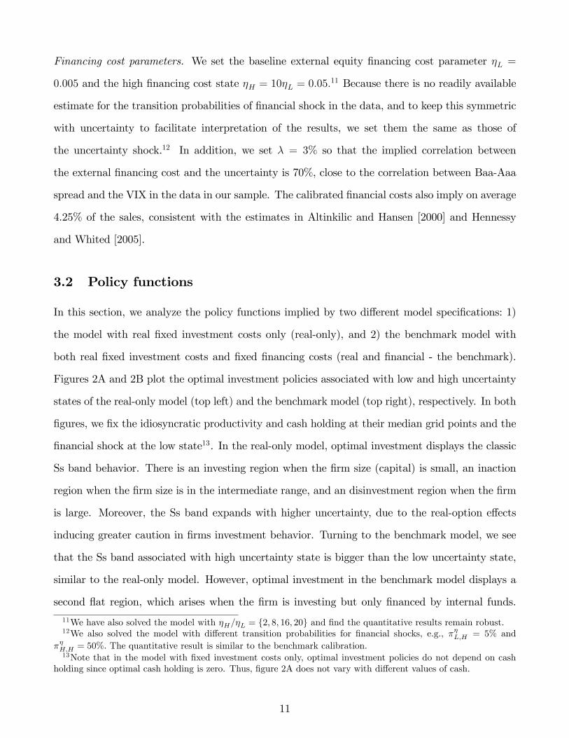
Financing cost parameters. We set the baseline external equity financing cost parameter ηL =

0.005 and the high financing cost state ηH = 10ηL = 0.05.11 Because there is no readily available

estimate for the transition probabilities of financial shock in the data, and to keep this symmetric

with uncertainty to facilitate interpretation of the results, we set them the same as those of

the uncertainty shock.12 In addition, we set λ = 3% so that the implied correlation between

the external financing cost and the uncertainty is 70%, close to the correlation between Baa-Aaa

spread and the VIX in the data in our sample. The calibrated financial costs also imply on average

4.25% of the sales, consistent with the estimates in Altinkilic and Hansen [2000] and Hennessy

and Whited [2005].

3.2 Policy functions

In this section, we analyze the policy functions implied by two different model specifications: 1)

the model with real fixed investment costs only (real-only), and 2) the benchmark model with

both real fixed investment costs and fixed financing costs (real and financial - the benchmark).

Figures 2A and 2B plot the optimal investment policies associated with low and high uncertainty

states of the real-only model (top left) and the benchmark model (top right), respectively. In both

figures, we fix the idiosyncratic productivity and cash holding at their median grid points and the

financial shock at the low state13. In the real-only model, optimal investment displays the classic

Ss band behavior. There is an investing region when the firm size (capital) is small, an inaction

region when the firm size is in the intermediate range, and an disinvestment region when the firm

is large. Moreover, the Ss band expands with higher uncertainty, due to the real-option effects

inducing greater caution in firms investment behavior. Turning to the benchmark model, we see

that the Ss band associated with high uncertainty state is bigger than the low uncertainty state,

similar to the real-only model. However, optimal investment in the benchmark model displays a

second flat region, which arises when the firm is investing but only financed by internal funds.

11We have also solved the model with ηH/ηL = {2, 8, 16, 20} and find the quantitative results remain robust.12We also solved the model with different transition probabilities for financial shocks, e.g., πηL,H = 5% and

πηH,H = 50%. The quantitative result is similar to the benchmark calibration.13Note that in the model with fixed investment costs only, optimal investment policies do not depend on cash

holding since optimal cash holding is zero. Thus, figure 2A does not vary with different values of cash.

11

This happens because firms are facing binding financial constraints (Et = 0), and are not prepared

to pay the fixed costs of raising external equity. When uncertainty is higher the real-option value

of this financing constraint is larger, so the binding constraint region is bigger. This shows how

real and financial constraints interact to expand the central region of inaction in Ss models.

Figure 2C plots the payout of the benchmark model (bottom left) of low and high uncertainty

by fixing the idiosyncratic productivity and cash holding at their median grid points and financial

shock at its low state. We see that firms both issue less equity and payout less in high uncertainty

state.

3.3 Benchmark model result

In this subsection, we compare panel regression data from the model simulation with specifications,

and also compare this to the real data. Specifically, we regress the rates of investment, employment

growth, cash growth and net payout (defined as positive payout minus the absolute value of equity

issuance) on the lagged growth of volatility (∆σt−1) at quarterly frequency, alongside a full set of

firm and year fixed-effects. Using the true volatility growth in the model allows us to mimic the

IV regressions for the real data regressions.

Table 4 starts in row (A) by presenting the results from the real data (discussed in section 5)

as a benchmark. As we see investment, employment and equity payouts significantly drop after

an increase in investment while cash holdings rises.14 Row (B) below presents the benchmark

simulation results (Real+financial frictions), and finds similar qualitative results with again drops

in investment, employment and equity payouts and rising cash holdings15. In Row (C) we turn

to the classic real frictions only model and see that the impact of uncertainty on investment and

employment growth falls from -0.077 to -0.042 and -0.027 to -0.014 respectively. This implies a

finance-uncertainty-multiplier of 1.83 (=0.077/0.042) for investment and 1.95 (=0.027/0.014) for

employment. So introducing financial frictions to the classic uncertainty model roughly doubles

the impact of uncertainty shocks.

14All results in this table are significant at the 1% (with firm-clustered standard errors), hence we do not reportt-statistics for simplicity.15The real results (Row A) and benchmark results (Row B) have similar quantitative magnitudes noting we did

not calibrate our parameters to meet these moments.

12

In Row (D) we instead simulate a model with just financial frictions, and interestingly we still

get a (smaller) negative impact of uncertainty on investment and employment, driven by firms

desire to hoard cash when uncertainty increases, alongside a (larger) impact on increasing cash

and cutting dividends. Hence, both the “real only”and “financial only”adjustment cost models

have similar implications that uncertainty shocks reduce investment, employment and dividends

and increase cash holdings. But, the real model has larger real (investment and employment)

impacts and smaller financial (dividend and cash impacts). Finally, Row (E) models firms with

no adjustment costs, resulting in very small positive Oi-Hartman-Abel impacts on investment and

employment, no cash impacts (without financial costs cash is zero), and large dividend impacts

due to extreme fluctuations in equity payouts.


3.4 Inspecting the mechanism

In this section, we inspect the model mechanism by first studying the impulse responses of the real

and financial variables in the benchmark model and then compare them to the real-only model

and the model with fixed financial costs only (financial-only). Furthermore, we also run panel

regressions in different model specifications to understand the marginal effect of real and financial

frictions.

3.4.1 Impulse responses

To simulate the impulse response, we run our model with 30, 000 firms for 800 periods and then

in quarter zero kick uncertainty and/or financing costs up to its high level in period 0 and then

let the model to continue to run as before. Hence, we are simulating the response to a one period

impulse and its gradual decay (noting that some events - like the 2007-2009 financial crisis - likely

had more persistent initial impulses).

Uncertainty shocks Figure 3 plots the impulse responses of the real and financial variables

of the benchmark model to a pure uncertainty shock. Starting with the classic “real adjustment

13

cost”only model (black line, x symbols) we see a peak drop in output of 1.3% and a gradual return

to trend. This is driven by drops and recoveries in capital, labor and TFP. Capital and labor drop

and recover due to increased real-option effects leading firms to pause investing (and thus hiring

by the complementarity of labor and capital), while depreciation and attrition continues to erode

capital and labor stocks. TFP falls and recovers due to the increased mis-allocation of capital and

labor after uncertainty shocks - higher uncertainty leads to more rapid reshuffl ing of productivity

across plants, which with reduced investment and hiring leads to more input mis-allocation.

Turning to the benchmark model (red line, triangle symbols) with “real and financial

adjustment costs” we see a much larger peak drop in output of 2.4%, alongside larger drops

in capital and labor. This is driven by the interaction of financial costs with uncertainty which

generates a desire by the firms to increase cash holdings when uncertainty is high. Hence, we again

see that adding financial costs to the classic model roughly doubles the impact of uncertainty

shocks.

Finally, the model with only “financial adjustment costs”(blue line, circles) leads to a similar

1.3% peak drop in output. This is driven by a similar mix of a drop in capital as financial

adjustment costs leads firms to hoard cash after an uncertainty shock, labor also drops (since

this is complementary with capital), as does TFP due to less investment and hiring raising mis-

allocation. The one notable difference in the impact of uncertainty shocks with real vs financial

adjustment costs is the time profile on output, capital and labor. Real costs lead to a sharp drop

due to the Ss band expansion which freezes investment after the shock, but with a rapid bounce-

back as the Ss bands contract and firms realize pent-up demand for investment. With financial

costs the uncertainty shock only reduces investment by firms with limited internal financing, but

this impact is more durable leading to a slower drop and recovery.

Financial shocks Figure 4 in contrast analyzes the impact of a pure financial shock - that is

a shock to the cost of raising external finance, η, in equation (8) - for the simulation with real,

financial and real+financial adjustment costs.

Starting first with real adjustment costs only (black line, x symbol) we see no impact because

there are no financial adjustment costs in this model. Turning to the financial frictions but no

14

real frictions model (blue line, circle symbols) we see only small impacts of financial shocks of

0.8% on output. The reason is with financial (but no real) frictions firms can easily save/dis-save

in capital, so they are less reliant on external equity. Finally, in the benchmark model (red line,

triangle symbols) we see by far the largest impact, with a drop in output of up to 2%, with similar

falls in capital and labor. The reason is intuitive - if financial costs are temporarily increased

firms will postpone raising external finance for investment, which reduces the capital stock and

hence labor (by complementarity with capital). TFP also shows a more modest drop due to the

increase in mis-allocation (as investment falls), although this is smaller than for an uncertainty

shock as firm-level TFP does not increase in volatility.16 Hence, even for financial shocks there is

a multiplier effect or about 2 between real and financial frictions.

Combined Uncertainty and Financial Shocks As Stock and Watson [2012] suggest

combined financial and real shocks are a common occurrence, and indeed these both occurred in

2007-2009, so we examine the impact of this in Figure 5. This plots the impact in the benchmark

model of an uncertainty shock (black line, + symbols), a financial shock (blue line, circle symbols)

and both shocks simultaneously (red line, triangle symbols).

The main result from Figure 5 is that both uncertainty and financial shocks individually lead

to drops in output, capital, labor and TFP of broadly similar sizes (financial shocks cut capital

and labor a bit more, uncertainty cuts aggregate TFP more). But collectively their impact is

significantly larger - for example, the drop in output from an uncertainty or financial shock alone

is 2.4% and 2.3% respectively, while jointly they lead to an output fall of 4%. This highlights that

combined financial and uncertainty shocks lead to substantially larger drops in output, investment

and hiring, alongside increases in cash holdings and reductions in equity payouts. As we saw in

Figure 1 this occurred in 2007-2009, suggesting modeling this as a joint finance-uncertainty shock

in a model will come closer to explaining the magnitude of this recession.

16This financial shock leads to about 1/4 of the drop in aggregate TFP of an uncertainty shock model becausewith financial shocks only investment and hiring slows, while with uncertainty TFP also becomes more volatile (soin the cross-section the correlation between K and L with A drops much faster).

15

3.4.2 Robustness

In this section we consider - changes in parameter values, general equilibrium and debt financing.

These are plotted in Figure 6 and Table (A1)

Changes in parameter values We start by evaluating one-by-one changes a series of the

parameter values listed in Table 2. The broad summary is that while the quantitative results

vary somewhat across different parameter values, the qualitative results are robust - uncertainty

shocks lead to drops and rebounds in output, capital and labor (alongside rises in cash and drops

in equity payouts), and these are roughly doubled by adding in financial adjustment costs.

In particular, we lower the high financing-cost-state-to-low-cost-state ratio (ηH/ηL ) from 10

to 5 (while keeping the low financial cost state ηL = 0.005). This leads to a similar drop in output

but with a faster recovery as it is now less expensive for constrained firms to finance investment

(dark blue line with squares, Figure 6). Next, rather than set the transition probabilities of the

financial shock to be the same as the uncertainty shock we set πσL,H = 0.05 and πσH,H = 0.5, which

implies that financial shocks expected every 5 years and the average time of the economy in high

financing cost state is 10% (similar to the calibration of the credit shocks in Khan and Thomas

[2013]). As we see (black line, circles) this leads to a very similar drop but faster recovery from

the uncertainty-finance shock because the finance shock is now less persistent.

General equilibrium Currently the model is in a particular equilibrium setting. A general

equilibrium set-up would require a Krusell and Smith [1998] type of model with its additional

loop and simulation to solve for prices and expectations. In prior work, for example Bloom et al.

[2016], this reduced the impact of uncertainty shocks by around 1/3 but did not radically change

their character. The reason is two-fold: first, prices (interest rates and wages) do not change

substantially over the cycle, and second the Ss nature of the firms’ investment decision makes

the policy correspondence insensitive in the short-run to price changes. However, to investigate

this we do run a pseudo-GE experiment, whereby we allow prices to change by an empirically

realistic amount after an uncertainty shocks. In particular, we allow interest rates to 1% lower

during periods of high uncertainty. So far we find broad robustness of our results on the impact

16

of uncertainty shocks with a similar sized drop but somewhat faster rebound (light-blue line with

triangles in Figure 6).

Debt financing In the model we examine equity financing and ignored debt to reduce the state

space of the model. We can also simulate a model with both debt and equity financing, and as we

show in this section the results are broadly similar. Our intuition was that when debt is collateral

constrained, both margins of debt and equity financing are costly for firms, hence frictions on debt

and equity altogether amplify the impact of uncertainty shocks.

Specifically, at the beginning of time t, firms can issue an amount of debt, denoted as Bt,

which must be repaid at the beginning of period t + 1. The firm’s ability to borrow is bounded

by the limited enforceability as firms could default on their obligations. Following Hennessy and

Whited [2005], we assume that the only asset available for liquidation is the physical capital Kt+1.

In particular, we require that the liquidation value of capital is greater than or equal to the debt

payment. It follows that the collateral constraint is given by

Bt+1 ≤ ϕKt. (11)

The variable 0 < ϕ < 1 affects the tightness of the collateral constraint, and therefore, the

borrowing capacity of the firm. Due to the collateral constraint, the interest rate, denoted by rf ,

is the risk-free rate.

Taxable corporate profits are equal to output less capital depreciation and interest expenses:

Πt−δKt−rfBt. It follows that the firm’s payout before equity financing cost (Et) as operating profit

minus investment in capital, cash accumulation and change in debt, less investment adjustment

costs

Et = (1− τ) Πt + τδKt + τrfBt − It −Ht −Gt +Bt+1 − (1 + rf )Bt, (12)

in which τ is the corporate tax rate, τδKt is the depreciation tax shield, τrfBt is the interest tax

shield. The external equity financing cost remains the same as in the benchmark model. We set

the liquidation value ϕ = 0.85 following Hennessy and Whited [2005] and the tax rate τ = 0.2

following Gomes and Schmid (2010). Note that in the model debt derives value from substituting

17

costly equity financing while not from the standard tax shield benefit in the finance literature. We

see in Figure 6 a somewhat smaller initial drop as firms can substitute debt for equity financing

(green line, + symbols), but a slightly more persistent impact of because of debt hangover.

4 Data and Instruments

We first describe the data and variable construction, then the identification strategy.

4.1 Data

Stock returns are from CRSP and annual accounting variables are from Compustat. The sample

period is from January 1963 through December 2016. Financial, utilities and public sector firms

are excluded (i.e., SIC between 6000 and 6999, 4900 and 4999, and above 9000). Compustat

variables are at the annual frequency. Our main firm-level empirical tests regress changes in

real and financial variables on 12-month lagged changes in uncertainty (i.e., lagged uncertainty

shocks), where the lag is both to reduce concerns about contemporaneous endogeneity and because

of natural time to build delays. Moreover, our main tests include both firm and time (calendar

year) fixed effects. The regressions of changes in outcomes on lagged annual changes in uncertainty

restricts our sample to firms with at least 3 consecutive non-missing data values. The firm fixed

effect further eliminates singletons. To ensure that the changes are indeed annual, we require a 12

month distance between fiscal-year end dates of accounting reports from one year to the next.

In measuring firm-level uncertainty we employ both realized annual uncertainty from CRSP

stock returns and option-implied uncertainty from OptionMetrics. Realized uncertainty is the

standard-deviation of daily cum-dividend stock returns over the course of each firm’s fiscal year

(which typically spans roughly 252 trading days).17 For implied volatility we use the 252-day

average of daily implied volatility values fromOptionMetrics. Data fromOptionMetrics is available

starting January 1996. Our daily implied volatility data corresponds to at-the-money 365-day

17We drop observations of firms with less than 200 daily CRSP returns in a given fiscal year. Our sample usessecurities appearing on CRSP for firms listed in major US stock exchanges (EXCHCD codes 1,2, and 3 for NYSE,AMEX and the Nasdaq Stock Market (SM)) and equity shares listed as ordinary common shares (SHRCD 10 or11).

18

forward call options. Additional information about OptionMetrics, Compustat, and CRSP data

is provided in Appendix ( B).

For changes in variables we define growth following Davis and Haltiwanger [1992], where for

any variable xt this is ∆xt = (xt − xt−1)/(12xt + 1

2xt−1) , which for positive values of xt and

xt−1 yields growth rates bounded between -2 and 2. The only exceptions are CRSP stock returns

(measured as the compounded fiscal-year return of daily stock returns RET from CRSP) and

capital formation. For the latter, investment rate (implicitly the change in gross capital stock) is

defined as Ii,t =CAPEXi,tKi,t−1

where K is net property plant and equipment, and CAPEX is capital

expenditures. The changes and ratios of real and financial variables are then all winsorized at the

1 and 99 percentiles.

Our main tests include standard controls used in the literature on both real investment and

capital structure. In particular, in addition to controlling for the lagged level of Tobin’s Q we follow

Leary and Roberts [2014] and include controls for lagged levels of firm tangibility, book leverage,

return on assets, log sales, and stock returns. The Appendix ( B) details the construction of these

variables.

4.2 Identification Strategy

Our identification strategy exploits firms’differential exposure to aggregate uncertainty shocks in

energy, currency, policy, and treasuries to generate exogenous changes in firm-level uncertainty.

The idea is that some firms are very sensitive to, for example, oil prices (e.g. energy intensive

manufacturing and mining firms) while others are not (e.g. retailers and business service firms), so

that when oil-price volatility rises it shifts up firm-level volatility in the former group relative to the

latter group. Likewise, some industries have different trading intensity with Europe versus Mexico

(e.g. industrial machinery versus agricultural produce firms), so changes in bilateral exchange

rate volatility generates differential moves in firm-level uncertainty. Finally, some industries - like

defense, health care and construction - are more reliant on the Government, so when aggregate

policy uncertainty rises (for example, because of elections or government shutdowns) firms in these

industries experience greater increases in uncertainty.

19

Our estimation approach is conceptually similar to the classic Bartik identification strategy

which exploits different regions exposure to different industry level shocks, and builds on the paper

by Stein and Stone [2013].

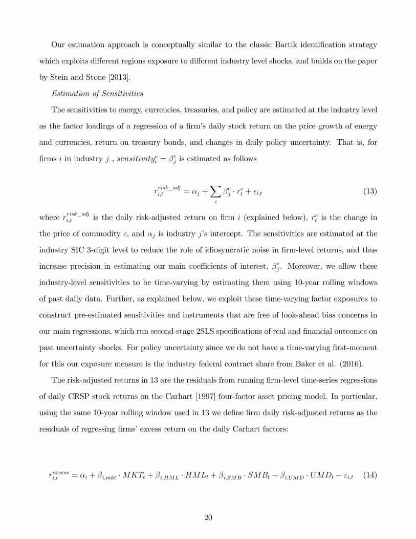
Estimation of Sensitivities

The sensitivities to energy, currencies, treasuries, and policy are estimated at the industry level

as the factor loadings of a regression of a firm’s daily stock return on the price growth of energy

and currencies, return on treasury bonds, and changes in daily policy uncertainty. That is, for

firms i in industry j , sensitivityci = βcj is estimated as follows

rrisk_adji,t = αj +

∑c

βcj · rct + εi,t (13)

where rrisk_adji,t is the daily risk-adjusted return on firm i (explained below), rct is the change in

the price of commodity c, and αj is industry j’s intercept. The sensitivities are estimated at the

industry SIC 3-digit level to reduce the role of idiosyncratic noise in firm-level returns, and thus

increase precision in estimating our main coeffi cients of interest, βcj. Moreover, we allow these

industry-level sensitivities to be time-varying by estimating them using 10-year rolling windows

of past daily data. Further, as explained below, we exploit these time-varying factor exposures to

construct pre-estimated sensitivities and instruments that are free of look-ahead bias concerns in

our main regressions, which run second-stage 2SLS specifications of real and financial outcomes on

past uncertainty shocks. For policy uncertainty since we do not have a time-varying first-moment

for this our exposure measure is the industry federal contract share from Baker et al. (2016).

The risk-adjusted returns in 13 are the residuals from running firm-level time-series regressions

of daily CRSP stock returns on the Carhart [1997] four-factor asset pricing model. In particular,

using the same 10-year rolling window used in 13 we define firm daily risk-adjusted returns as the

residuals of regressing firms’excess return on the daily Carhart factors:

rexcessi,t = αi + βi,mkt ·MKTt + βi,HML ·HMLt + βi,SMB · SMBt + βi,UMD · UMDt + εi,t (14)

20

where rexcessi,t is firm i’s daily CRSP stock return (including dividends and adjusted for delisting)

in excess of the t-bill rate, MKT is the CRSP value-weighted index in excess of the risk free rate,

HML is the book-to-market factor, SMB is the size factor, UMD is the momentum factor. These

factor data are obtained from CRSP.

We adjust returns for risk to address concerns over whether the sensitivities to energy,

currencies, treasuries, and policy (βcj in equation 13) are capturing systematic "risks" rather than

exposure to the prices of interest. Our main results are fairly similar when we use longer or shorter

rolling windows, of 15 and 5 years, in both 13 and 14 and raw or risk adjusted returns.

The daily independent variables in 13 are the growth in crude-oil prices (which proxies for

energy shocks), growth in the exchange rates of 7 widely traded currencies defined as "major"

currencies by the Federal Board 18, the return on the US 10-year treasury note 19, and the growth

in economic policy uncertainty from Baker et al. [2016]. For these 10 aggregate market price shocks

(oil, 7 currencies, treasuries, and policy) we need not only their daily returns (for calculating the

sensitivities βcj in equation 13) but also their implied volatilities σct as measures of aggregate sources

of uncertainty.

Construction of Instruments

To instrument for firm-level uncertainty shocks, ∆σi,t, we also require data on aggregate

uncertainty shocks, ∆σct . We define the annual uncertainty on oil, currency, and 10-year treasuries

as the 252-day average of daily implied volatility of oil and currencies from Bloomberg and for

treasuries we use the 252-day average of daily implied volatility for the 10-year US Treasury Note

from the Cboe/CBOT (ticker TYVIX). Likewise, for annual policy uncertainty we employ the

365-day average of the US economic policy uncertainty index from Baker et al. [2016]. These 10

annual aggregate uncertainty measures, σct , are used in constructing cross-industry exposures to

aggregate uncertainty shocks, | βc,weightedj | ·∆σct .

We do this in two steps. First, we adjust the factor sensitivities estimated in 13 for their

18see http://www.federalreserve.gov/pubs/bulletin/2005/winter05_index.pdf . These include: the euro,Canadian dollar, Japanese yen, British pound, Swiss franc, Australian dollar, and Swedish krona. Each one of thesetrades widely in currency markets outside their respective home areas, and (along with the U.S. dollar) are referredto by the Board staff as major currencies.19the treasury return is estimated from the first-order approximation of duration, i.e., by multiplying the first

difference of the yield by minus 1.

21

http://www.federalreserve.gov/pubs/bulletin/2005/winter05_index.pdf

statistical significance. In particular, within each industry we construct significance-weighted

sensitivities βc,weightedj = ωcj · βcj, where the first term is a sensitivity weight constructed from the

ratio of the absolute value of the t-statistic of each instrument’s sensitivity to the sum of all t-

statistics in absolute value of instruments within the industry, ωcj =abs(tcj)c∑abs(tcj)

. Thus, we adjust the

sensitivities within each industry by their statistical power in 13. However, in constructing the

weights ωcj we first set to zero each individual t-statistic for which the corresponding sensitivity is

statistically insignificant at the 10% level. This is done both before taking the absolute value of

each t-statistic and the sum of their absolute values. Thus, the significance-weighted sensitivities

βc,weightedj can be zero for certain industries. However, recalling that the raw sensitivities βcj in

13 are estimated in rolling windows, the significance-weighted sensitivities βc,weightedj need not be

zero at every moment in time. Indeed, our sample shows that 3-SIC industries fluctuate both in

their extensive and intensive exposure to the each of our 10 instruments over time. Our weighting

scheme captures and exploits both margins.

Second, we construct 10 composite terms | βc,weightedj | ·∆σct , which we refer to as the

industry-by-year exposure for uncertainty shocks, where the first term is the absolute value of the

significance-weighted sensitivity explained above and ∆σct is the annual growth in the aggregate

uncertainty of the instrument. Thus, our instrumental variables estimation uses 10 instruments,

the oil exposure term, the seven currencies exposure terms, the 10-year treasury exposure term,

and the policy-uncertainty exposure term. These 10 composite industry-by-year exposure for

uncertainty shocks are the instruments used in our 2SLS regressions that instrument for firm-level

uncertainty shocks.

In terms of timing, in the first stage when we regress annual firm-level uncertainty ∆σi,t

shocks on the 10 composite exposure terms | βc,weightedj | ·∆σct , aggregate uncertainty shocks ∆σct

are contemporaneous growths but the exposures βc,weightedj are always estimated using information

prior to the uncertainty growth, in particular with a lag of 24 months. For example, for a firm

with a fiscal-year end in December 2012, the exposures are estimated using 13 and a window of

10-years of daily data ending with information up to December of 2010 (i.e., lag of 24 months),

and the growth ∆σct is the change in the annual option-implied uncertainty measured over the

22

course of 2011 to that of 2012.

Finally, to disentangle second moment effects from first moment effects of our 10 instruments,

we also include as controls in the second stage of the 2SLS regressions the exposure to the returns

of each instrument (i.e., first moment controls). That is, in the regressions we also include 10 first

moment composite terms βc,weightedj · rct .20 Thus, our empirical examination focuses on the effects

of uncertainty shocks above and beyond first moment effects. At the firm-level, our main set of

controls further includes each individual firms’measure of first moment effects, i.e., the CRSP

stock return of the firm, ri,t (which accounts for discount rate channel effects), yet our focus is on

the effects of the instrumented firm-level uncertainty shocks, ∆σi,t

5 Empirical findings

We start by examining how volatility shocks relate to firm-level capital investment rates, followed

by other real outcomes -intangible capital investment, employment, and cost of goods sold- and

then by financial variables -debt, payout, and cash holdings.

5.1 Investment results

Table 5 examines how uncertainty influences future capital investment rates. Column 1 presents

the univariate Ordinary Least Squares regression results of investment rate on lagged annual

realized stock return volatility shocks. We observe highly statistically significant coeffi cients (t-

stat of 19.89) on return volatility, showing that firms tend to invest more when their firm-specific

uncertainty is low. Column 4 presents the corresponding OLS univariate regression results of

investment rate on lagged firm-level implied volatility shocks (from OptionMetrics). The sign of

the coeffi cient is consistent with realized volatility shocks, but the size is more than twice as large,

potentially because implied volatility is a better measure of uncertainty.21

20For economic policy uncertainty we measure rct as growth from one year to the next in the 4-quarter averageof the level of government expenditure as a share of GDP. For currencies, oil, and treasuries returns rct are the252-day average of daily returns.21We reestimate both specifications in columns (1) and (4) on a common sample of 17,487 observations in table

(A4) and find the realized and implied volatility coeffi cients are -0.033 and -0.079, suggesting the three fold differencearises from the difference in variables rather than samples (e.g. realized volatility shocks have a standard deviation

23

One obvious concern with these OLS regressions is endogeneity - for example, changes in firms’

investment plans could change stock-prices. Using lagged uncertainty will help to address this to

some extent, but given stock prices are forward looking this is unlikely to fully address the concerns.

So we try to address these endogeneity concerns with our instrumentation strategy. In particular,

columns 2 and 3 instrument lagged realized volatility using the full set of 10 instruments while

columns 5 and 6 instrument lagged implied volatility. Columns 2 and 5 are univariate while 3 and

6 are multivariate with a full set of controls. In all cases we see find that uncertainty shocks lead

to significant drops in firm-level investment.

The point estimates of the coeffi cients on instrumented uncertainty shocks with the full set

of controls are roughly of comparable magnitude to the univariate OLS point estimates (e.g.,

columns 3 and 1). Our full set of lagged controls includes Tobin’s Q, log sales and stock-returns

to control for firm moment shocks, as well as book leverage, profitability (return on assets) and

tangibility to control for financial conditions. Our multivariate specifications also include firm and

time fixed effects and cluster standard errors at the 3-SIC industry (which is the same level at

which our instrumentation strategy estimates factor exposures). In all instrumented cases, rises

in uncertainty is a strong predictor of future reductions in capital investment rates.

In terms of magnitudes the results imply that a two-standard deviation increase in realized

volatility (see the descriptive statistics in Table A1) would reduce investment by between 4% to

6% (using the results from our preferred multivariate specifications in column (3) and (6)). This

is moderate in comparison to firm-level investment fluctuations which have a standard deviation

of 24.7%, but is large when considering that annual investment rates drop about 2% or 6% during

recessions as show in Figure 1.


5.1.1 First stage results

The first stage instrumental investment results are shown in table 6. Columns (1) and (2) report

the first stages for the univariate IV columns (2) and (4) from table 5. We see that the F-

of 0.3 vs 0.2 for implied volatility shocks).

24

statistics indicate a well identified first stage with values of 166.8 and 78.79 for the Cragg-Donald

(CD) F-Statistics (robust standard-errors), and 19.33 and 13.20 for the Kleibergen-Paap (KP) F

statistic (SIC-3 digit clustering). We also find the Hansen over-identifying test does not reject the

validity of our instruments with p-values of 0.246 and 0.680. As another check of our identification

strategy we would like to see that each of our instruments is individually positively, and generally

significantly correlated with uncertainty shocks. Indeed, we see in columns (1) and (2) that all 10

instruments are positively and mostly significant in the first stage.

We repeat the above examination but adding our full set of controls, columns (3) and (4) present

the first stage for the multivariate IV regressions of columns (3) and (6) from table 5. Even when

we add our full set of controls we see a well satisfied relevance condition, with CD and KP F-stats

of 179.2, 60.41 18.02 and 11.49 respectively, and non-rejected Sargan-Hansen validity test p-values

of 0.873 and 0.988. Moreover, each instrument remains individually positively correlated with

uncertainty shocks.

[Inset Table 6 here]

5.2 Intangible capital, Employment, and sales

Table 7 examines the predictive and causal implications of uncertainty shocks on the growth of

other real outcomes. In particular, Panel A examines investment in intangible capital (as measured

by expenditure on general and administration and R&D, which extends the approach of Eisfeldt

and Papanikolaou (2013)), Panel B examines employment, and Panel C examines the cost of goods

sold. In each panel we present the same 6 specification results presented for investment in Table

5. but to preserve space we drop the point coeffi cient estimates on controls and keep only the

estimates on lagged uncertainty shocks.

The three panels show that realized and implied volatility shocks are negatively related to

future changes in intangible capital investment, employment, and cost of goods sold. As with

investment, these regressions show a strong first-stage with F-statistics above 10 in all multivariate

specifications that include a full set of controls, columns (3) and (6). In our preferred specification

of column (3), which instruments realized lagged uncertainty shocks, both intangible capital

25

investment and cost of good sold drop upon higher realized uncertainty (significant at the 5

and 1 percent, respectively), while the response of employment is negative but not statistically

significant.


Overall, the three panels confirm the robustness of the causal impact of uncertainty shocks on

real firm activity, even in the presence of extensive first-moment and financial condition controls,

plus an extensive instrumentation strategy for uncertainty shocks.

5.3 Financial variables

Table 8 examines how firm uncertainty shocks affect future changes in financial variables. In

particular, Panel A examines total debt, Panel B dividend payout, and Panel C cash holdings.

Panel A indicates that increases in uncertainty reduce the willingness of firm’s to increases their

overall debt. The correlations are strong and significant in both the OLS and instrumental variable

regressions. Panel B indicates that firm’s take a more cautious financial approach toward corporate

payout. Consistent with a precautionary savings motive, rises in firm uncertainty causes a large

reduction in cash dividend payout. Similarly, Panel C further evidences a precautionary savings

channel as cash holdings increase upon large uncertainty shocks. In particular, firms accumulate

cash reserves and short-term liquid instruments following uncertainty rises.

For the preferred specifications in columns (3) and (6) all three panel show highly significant

point estimates (at the 5% and 1%), strong first stage F-statistics, and non-rejections on the

Sargan-Hansen over-identifying test. This highlights that our instrumental strategy based on

exchange rate and factor price volatility works well not only for real outcomes but also for financial.


5.4 Instrument and credit supply robustness

In Appendix Table A2 we investigate the main multivariate investment results dropping each

instrument one-by-one in columns (2) to (9) to show our results are not being driven by any

26

particular instrument (noting in column (10) we drop the oil and treasury instruments together to

allow us to extend our sample size to 42,732)22. As we see across the columns the first stage results

for investment are impressively robust - the tougher KP F-test test is in the range of 13.34 to 20.35

in all specifications (the CD F—test is always above 100), and the Hansen over-identifying test does

not reject in any specification with p-values of 0.8 or above. Although in column (10) cost of goods

sold does not respond to uncertainty shocks, all other real and financial firm-outcomes examined

in baseline column (1) are robust. Taken together, the results across all columns indicate that our

identification results are not driven by one particular instrument, but instead are driven by the

combined identification of energy, exchange rate, policy, and treasury uncertainty driving firm-

level uncertainty fluctuations and firm decisions. This suggests that our identification strategy

will likely be broadly useful for a wide-range of models of the causal impact of uncertainty on firm

behavior.

[Insert Table A2 here]

In Appendix table A3 we investigate the robustness of the results to including additional firm-

level controls for financial constraints. One concern could be that uncertainty reduces financial

supply - for example, banks are unwilling to lend in periods of high uncertainty - which causes

the results we observe. To try to address this we include a variety of different controls for firms

financial conditions and show our baseline results are robust to this. In particular for both the

realized and implied volatility specifications we include controls for firm: CAPM-beta (defined as

the covariance of the firms daily returns with the market returns in the past year, scaled by the

variance of the market) in columns 2 and 2A, a broad set of firm financial constraint controls in

columns 3 and 3A - which include the lags for the Whited and Wu [2006] index, size and age

(SA) index of Hadlock and Pierce [2010], the Kaplan and Zingales [1997] index, reciprocal of total

assets, reciprocal of employees, and reciprocal of age -where age is the number of years since firm

incorporation-, the firms long-term credit rating from S&P in columns 4 and 4A (which consist of

a full set of dummies based on every possible credit rating category given to firms by S&P on long-

term debt, where the omitted dummy is for no credit ratings), and all of the previous measures22Oil and 10-year treasury daily implied volatility data starts in March 2003, whereas implied volatility data on

the Euro-USD bilateral exchange rate starts in 1999 and policy in 1985.

27

combined in columns 5 and 5A. In summary, as we can see from Table A3 including these financial

supply variables does not notably change our results. So while these are not perfect controls for

financial conditions, the robustness of our results to their inclusion suggests that financial supply

conditions are unlikely to be the main driver of our results.


Finally, in Table A4 we re-examine our main investment Table 5 but holding the sample of

firm-time observations to be the same across specifications (1) to (6). In particular, our sample is

constrained by the availability of OptionMetrics data on firm-level implied volatility, which gives a

total of 17,487 observations across all columns. Compared to the main Table 5 the point estimates

on the coeffi cients are largely comparable in both magnitude and statistical significance. Therefore,

differences in point estimates across specifications (2SLS vs OLS, univariate vs multivariate, and

realized vs implied volatility shocks) are primarily due to the underlying specifications themselves

and not due to differences in sample size.


5.5 The finance uncertainty multiplier

Finally, Table 9 shows the results from running a series of finance-uncertainty interactions on

the data during the core Jan. 2008-Dec. 2009 period of the financial crisis. By running double

and triple interaction of uncertainty with financing frictions we attempt to tease out the finance-

uncertainty multiplier effects examined in the model of section 2. In particular, Table 9 examines

the impact of realized volatility shocks on investment for financially constrained and unconstrained

firms during financial crisis and non-crisis years. We do this by running the following specification

and subsets of it:

Ii,t/Ki,t−1 = β0 + β1∆σi,t−1 + β2Dcrisis_year,t

+β3Dcrisis_year,t ·∆σi,t−1 + β4Dfin.constrained,i,t−1 + β5Dfin.constrained,i,t−1 ·∆σi,t−1

+β6Dcrisis_year,t ·Dfin.constrained,i,t−1 + β7Dcrisis_year,t ·Dfin.constrained,i,t−1 ·∆σi,t−1 (15)

28

where ∆σi,t−1is firm i′s growth of realized annual vol from year t − 2 to t − 1, Dcrisis_year,t

is a dummy that takes value of 1 for all firm fiscal-year observations of investment rate ending

in calendar years 2008 and 2009, i.e., core years of the financial crisis which comprise the core

months of the great recession in which firms would have observed at least 6 months of heightened

financial frictions in their annual accounting reports, zero otherwise, and Dfin.constrained,i,t−1is a

dummy that takes value of 1 for firms classified as financially constrained (e.g., according to

Whited-Wu index) in year t− 1, zero otherwise. The coeffi cient β7 indicates whether the effect of

uncertainty on investment is different for financially constrained firms during crisis years relative to

unconstrained firms. Employing dummies to classify firms into groups rather than using firm-level

financing constraint measures in our interaction terms facilitates the comparison of key coeffi cients

β3, β7 across different noisy estimates of financing constraints.23

Column (1) presents our baseline 2SLS multivariate specification with full set of controls

presented in Table 5 column (3). Column (2) interacts past uncertainty shocks with the

contemporaneous crisis dummy, Dcrisis_year,t. The regression indicates that the effects of

uncertainty shocks on investment are fully attributable to the period of large uncertainty spikes

and large rises in financing frictions seen in the core crisis years of the great recession, as seen

by the highly significant interaction term Dcrisis_year,t · ∆σi,t−1 which subsumes the effect of the

uncertainty shock alone. This is consistent with the main thesis in this paper that financial

constraints substantially amplify the impact of uncertainty shocks.


To disentangle and further understand these financing frictions vs uncertainty effects, columns

(3) to (8) run the full difference-in-difference-in-difference specification in 15 , where we employ

a total of 6 proxies for financing frictions to classify firms into financially constrained and

unconstrained groups. For example, in column (4) using each firm’s financial constraint Whited-

Wu index at every fiscal year t − 1 we classify firms into constrained and unconstrained groups

using the 40 and 60 percentile cutoffs obtained from the cross-sectional fiscal-year distribution of

23There is a large literature on measuring firm-level financial constraints. Any proxies are usually subject tocritiques on whether they truly capture constraints or just noise. We employ a total of 6 different proxies to takerough cuts to our Compustat data. We thank Toni Whited for suggestions on this front, e.g., adding the SA index.

29

the given index. We consider a firm constrained if its t − 1 index value is equal to or greater

than the 60 percentile and unconstrained if equal to or less than the 40 percentile. We exclude

firm-time observations in the middle 50+/-10 percentiles to increase precision in the classification

of firms.24 We do this in all but the S&P credit-rating financial constraint measure, column (3).

Here we follow Duchin et al. [2010] and consider a firm constrained if it has positive debt and

no bond rating and unconstrained otherwise (which includes firms with zero debt and no debt

rating).25

In sum the 6 measures of financial constraints are constructed using S&P ratings column

(3), Whited-Wu index column (4)„reciprocal of employees column (5), reciprocal of total assets

column (6), reciprocal of age column (7) in which age is defined as the number of years since firm

incorporation, and the SA index based on size and age of Hadlock and Pierce [2010] column (8). In

all specifications we include both firm and calendar-year fixed effects, and cluster standard errors

at the 3 digit SIC industry. All specifications include full set of controls of baseline specification

column (1).

Using the Whited-Wu index column (4) to classify firms, the results indicate that investment

rates drop upon larger uncertainty shocks (negative and significant β1 coeffi cient on uncertainty

shock ∆σi,t−1, at the 5%), the drop is more pronounced during the core crisis years of 2008 and

2009 (negative and significant β3 coeffi cient on the double interaction termDcrisis_year,t ·∆σi,t−1, at

the 1%), and the negative real effect on investment is amplified for ex-ante financially constrained

firms during the core crisis years (as determined by the negative and significant β7 coeffi cient on

the triple interaction term Dcrisis_year,t ·Dfin.constrained,i,t−1 ·∆σi,t−1, at the 5%).

Using other measures of financial constraints in columns (3) to (8) give similar inferences:

uncertainty matters (causally), it matters even more during periods of financial constraints, and

it matters most for the most ex-ante constrained firms. Hence, overall Table 9 provides important

empirical evidence in support of the testable predictions of the model of section 2 for an interactive

24Our inferences are similar if we expand or reduce the window of observations dropped in the middle: 50+/-15and/or 50+/-5 percentiles, i.e., comparing top vs bottom 30% and/or 45% of firms. Moreover, results are similarif we classify firms as ex-ante financially constrained or unconstrained using two-year past indexes of financialconstraints.25For ratings data we use Compustat-Capital IQ’s ratings data from WRDS, where ratings dummies are based

on variable SPLTICRM (S&P Domestic Long-Term Issuer Credit Rating).

30

effect of financial constraints and uncertainty in deterring firm investment activities during the

2008-2009 period of the financial crisis.

To show this graphically in the raw data Figure 7 plots investment rates for financially

constrained and unconstrained firms from 2003 to 2013. We normalize the investment rates of both

groups of firms to their respective values of investment rates in 2006. Financial constraints are

defined as a firm having short or long-term debt but no public bond rating (see, e.g., Faulkender and

Petersen [2006] and Duchin et al. [2010]). Volatility is the annual realized stock return volatility. It

is clear that constrained and unconstrained firms’investment rates track each other closely until

the Great Recession, at which point the constrained firms’ investment drop substantially more

than unconstrained firms. As uncertainty recedes post 2012 the gaps start to recede again as the

investment rates begin to converge. There are of course many ways to explain this difference (e.g.

small vs large firms), but it is at least consistent with the model of uncertainty shocks mattering

more for more financially constrained firms.

As a robustness Appendix Table A5 repeats the examination done in Table 9, but using option-

implied firm-level uncertainty shocks instead of realized uncertainty shocks. The inferences on the

economic importance of uncertainty shocks are robust to these forward-looking uncertainty data.


6 Conclusion

This paper studies the impact of uncertainty shocks on firms’ real and financial activity both

theoretically and empirically. We build a dynamic model which adds two key components: first,

real and financial frictions, and second, uncertainty and financial shocks. This delivers three key

insights. First, combining real and financial frictions roughly doubles the impact of uncertainty

shocks - this is the finance uncertainty multiplier. Second, combining an uncertainty shock with a

financial shock in this model increases the impact by about another two thirds, since these shocks

have an almost additive effect. Since uncertainty and financial shocks are highly collinear (e.g.

Stock and Watson 2012) this is important for modelling their impacts. Finally, in this model

31

uncertainty shocks not only reduce investment and hiring, but also raise firms cash holding, while

cutting equity payouts. Collectively, these predictions of a large impact of uncertainty shocks on

real and financial variables matches the evidence from the recent financial crisis.

We then use empirical data on U.S. listed firms to test the model using a novel instrumentation

strategy. Consistent with the testable implications, uncertainty shocks reduce firm investment

(tangible and intangible) and employment on the real side, and increase cash holdings, while

reducing payouts and debt on the financial side.

Taken together, our theoretical and empirical analyses show that real and financial frictions

are quantitatively crucial to explain the full impact of uncertainty shocks on real and financial

activity.

32

References

A. Abel and J. Eberly. Optimal investment with costly reversibility. Review of Economic Studies,63:581—593, 1996.

P. Alessandri and H. Mumtaz. Financial regimes and uncertainty shocks. QMW mimeo, 2016.O. Altinkilic and R. S. Hansen. Are there economies of scale in underwriting fees? evidence ofrising external financing costs. Review of Financial Studies, 13:191—218, 2000.

C. Arellano, Y. Bai, and P. J. Kehoe. Financial frictions and fluctuations in volatility. WorkingPaper, 2016.

P. Asquith and D. Mullins. Equity issues and offering dilution. Journal of Financial Economics,15:61—89, 1986.

R. Bachmann and C. Bayer. Wait-and-see business cycles? Journal of Monetary Economics, 60(6):704—719, 2013.

R. Bachmann and G. Moscarini. Business cycles and endogenous uncertainty. Working Paper,University of Notre Dame and Yale University, 2012.

S. Baker, N. Bloom, and S. Davis. Measuring economic policy uncertainty. Forthcoming QuarterlyJournal of Economics, 2016.

R. Bansal and A. Yaron. Risks for the long run: A potential resolution of asset pricing puzzles.Journal of Finance, 59:1481—1509, 2004.

R. Barro. Rare disasters and asset markets in the twentieth century. Quarterly Journal ofEconomics, 121(3):823—866, 2006.

S. Basu and B. Bundick. Uncertainty shocks in a model of effective demand. NBER WorkingPaper No. 18420, 2017.

D. Berger, I. Dew-Becker, and S. Giglio. Contractionary volatility or volatile contractions?Working paper, Northwestern University, 2016.

B. Bernanke and M. Gertler. Agency costs, net worth, and business fluctuations. AmericanEconomic Review, 79(1):14—31, 1989.

B. S. Bernanke. Irreversibility, uncertainty, and cyclical investment. Quarterly Journal ofEconomics, 98(1):85—106, 1983.

G. Bertola and R. J. Caballero. Kinked adjustment costs and aggregate dynamics. NBERMacroeconomics Annual, 5:237—296, 1990.

S. Bigio. Endogenous liquidity and the business cycle. American Economic Review, 105(6):1883—1927, 2015.

N. Bloom. The impact of uncertainty shocks. Econometrica, 77:623—685, 2009.N. Bloom, M. Floetotto, N. Jaimovich, I. Saporta-Eksten, and S. Terry. Really uncertain businesscycles. National Bureau of Economic Research, Stanford University, 2016.

P. Bolton, H. Chen, and N. Wang. A unified theory of tobin’s q, corporate investment, financing,and risk management. Journal of Finance, 66:1545—1578, 2011.

P. Bolton, H. Chen, and N. Wang. Market timing, investmentand risk management. Journal ofFinancial Economics, 109:40—62, 2013.

R. Caballero, E. Engel, and J. Haltiwanger. Plant-level adjustment and aggregate investmentdynamics. Brookings Papers on Economic Activity, 2:1—54, 1995.

M. Carhart. On persistence in mutual fund performance. Journal of Finance, 52,1:57—82, 1997.C. T. Carlstrom and T. S. Fuerst. Agency costs, net worth, and business fluctuations: Acomputable general equilibrium analysis. American Economic Review, 87(5):893—910, 1997.

G. Chen. Corporate savings, financingand investment with aggregate uncertainty shocks. WorkingPaper, Nanyang Technological University, 2016.

33

H. Chen, H. Wang, and H. Zhou. Stock return volatility and capital structure decisions. PBCSF-NIFR, Tsinghua University, 13,04, 2014.

H. Choe, R. Masulis, , and V. Nanda. Common stock offerings across the business cycle: Theoryand evidence. Journal of Empirical Finance, 1:3—31, 1993.

L. J. Christiano, R. Motto, and M. Rostagno. Risk shocks. American Economic Review, 104:27—65, 2014.

T. F. Cooley and V. Quadrini. Financial markets and firm dynamics. American Economic Review,91:1286—1310, 2001.

R. Cooper and J. Haltiwanger. On the nature of capital adjustment costs. Review of EconomicStudies, 73:611—633, 2006.

S. J. Davis and J. Haltiwanger. Gross job creation, gross job destruction, and employmentreallocation. The Quarterly Journal of Economics, MIT Press, 107,3:819—863, 1992.

H. DeAngelo, L. DeAngelo, and T. M. Whited. Capital structure dynamics and transitory debt.Journal of Financial Economics, 99:235—261, 2011.

A. K. Dixit and R. S. Pindyck. Investment under Uncertainty. Princeton: Princeton UniversityPress, Princeton, N.J, 1994.

R. Duchin, O. Ozbas, and B. Sensoy. Costly external finance, corporate investmentand thesubprime mortgage credit crisis. Journal of Financial Economics, 97:418—435, 2010.

A. Eisfeldt. Endogenous liquidity in asset markets. Journal of Finance, 59(1):1—30, 2004.A. Eisfeldt and T. Muir. Aggregate external financing and savings waves. Journal of MonetaryEconomics, 84:116—133, 2016.

I. Erel, B. Julio, W. Kim, and M. Weisbach. Macroeconomic conditions and capital raising. Reviewof Financial Studies, 25:341—376, 2012.

P. Falgelbaum, E. Schaal, and M. Taschereau-Dumouchel. Uncertainty traps. Forthcoming,Quarterly Journal of Economics, 2016.

M. Faulkender and M. Petersen. Does the source of capital affect capital structure? Review ofFinancial Studies, 19:45—79, 2006.

J. Fernandez-Villaverde, P. G. Quintana, J. F. Rubio-Ramirez, and M. Uribe. Risk matters: Thereal effects of volatility shocks. American Economic Review, 101,6:2530—61, 2011.

J. Fernandez-Villaverde, P. Guerron-Quintana, K. Kuester, and J. Rubio-Ramirez. Fiscal volatilityshocks and economic activity. American Economic Review, 105(11):3352âAS3384, 2015.

S. Gilchrist, J. Sim, and E. Zakrajsek. Uncertainty, financial frictions and investment dynamics.Boston University mimeo, 2014.

J. Gomes. Financing investment. American Economic Review, 65(2):467—494, 2001.F. Gourio. Disaster risk and business cycles. American Economic Review, 102(6):2734—2766, 2012.J. Graham. How big are the tax benefits of debt? Journal of Finance, 55(5):1901—1941, 2000.L. Guiso and G. Parigi. Investment and demand uncertainty. Quarterly Journal of Economics,114:185—227, 1999.

C. J. Hadlock and J. R. Pierce. New evidence on measuring financial constraints: Moving beyondthe kz index. The Review of Financial Studies, 23(5):1909—1940, 2010.

K. Handley and N. Limao. Trade and investment under policy uncertainty: Theory and firmevidence. NBER Working Paper 17790, 2012.

C. A. Hennessy and T. M. Whited. Debt dynamics. Journal of Finance, 60:1129—1165, 2005.C. A. Hennessy and T. M. Whited. How costly is external financing? evidence from a structuralestimation. Journal of Finance, 62:1705—1745, 2007.

C. A. Hennessy, A. Levy, and T. M. Whited. Testing q theory with financing frictions. Journalof Financial Economics, 83(3):691—717, 2007.

34

C. Ilut andM. Schneider. Ambiguous business cycles. American Economic Review, 104(8):2368—99,2014.

U. Jermann and V. Quadrini. Macroeconomic effects of financial shocks. American EconomicReview, 102(1):238—71, 2012.

K. Kahle and R. Stulz. Access to capital, investment, and the financial crisis. Journal of FinancialEconomics, 110(2):280—299, 2013.

S. Kaplan and L. Zingales. Do investment cash-flow sensitivities provide useful measures offinancing constraints? Quarterly Journal of Economics, 112:169—215, 1997.

A. Khan and J. Thomas. Idiosyncratic shocks and the role of nonconvexities in plant and aggregateinvestment dynamics. Econometrica, 76,2:395—436, 2008.

A. Khan and J. K. Thomas. Credit shocks and aggregate fluctuations in an economy withproduction heterogeneity. The Review of Financial Studies, 121(6):1055—1107, 2013.

R. King and S. Rebelo. Handbook of Macroeconomics. North-Holland, Amsterdam, Netherlands,1999. Resuscitating real business cycles.

P. Krusell and A. A. Smith. Income and wealth heterogeneity in the macroeconomy. Journal ofPolitical Economy, 106(5):867—896, 1998.

P. Kurlat. Lemons markets and the transmission of aggregate shocks. American Economic Review,103(4):1463—1489, 2013.

J. V. Leahy and T. Whited. The effect of uncertainty on investment: Some stylized facts. Journalof Money, Creditand Banking, 28:64—83, 1996.

M. T. Leary and M. R. Roberts. Do peer firms affect corporate financial policy? Journal ofFinance, 69(1):139—178, 2014.

G. Lee and R. W. Masulis. Seasoned equity offerings: Quality of accounting information andexpected flotation costs. Journal of Financial Economics, 92(3):443—469, 2009.

S. Lhuissier and F. Tripier. Do uncertainty shocks always matter for business cycles? CEPIIworking paper, 2016.

N. Moyen. Investment-cash flow sensitivities: Constrained versus unconstrained firms. Journal ofFinance, 59:2061—2092, 2004.

S. V. Nieuwerburgh and L. Veldkamp. Learning asymmetries in real business cycles. Journal ofMonetary Economics, 53:753—772, 2006.

A. Orlik and L. Veldkamp. Understanding uncertainty shocks and the role of the black swan.Working paper, NYU, 2015.

L. Pastor and R. Stambaugh. Liquidity risk and expected stock returns. Journal of PoliticalEconomy, 111:642—685, 2003.

L. Pastor and P. Veronesi. Uncertainty about government policy and stock prices. Journal ofFinance, 67:1219—1264, 2012.

R. G. Rajan and L. Zingales. What do we know about capital structure? some evidence frominternational data. Journal of Finance, 50:1421—1460, 1995.

V. Ramey and G. Ramey. Cross-country evidence on the link between volatility and growth.American Economic Review, 85,5:1138—51, 1995.

A. Rampini and S. Viswanathan. Collateral and capital structure. Journal of Financial Economics,109:466—492, 2013.

L. A. Riddick and T. M. Whited. The corporate propensity to save. Journal of Finance, 64:1729—1766, 2009.

T. Rietz. The equity premium: a solution. Journal of Monetary Economics, 22(1):117âAS131,1988.

C. Romer. The great crash and the onset of the great depression. Quarterly Journal of Economics,

35

105(3):597—624, 1990.G. Segal, I. Shaliastovich, and A. Yaron. Good and bad uncertainty: Macroeconomic and financialmarket implications. Journal of Financial Economics, 117:369—397, 2015.

L. Stein and E. Stone. The effect of uncertainty on investment, hiring and rd: causal evidencefrom equity options. Arizona State University mimeo, 2013.

J. Stock and M. Watson. Disentangling the channels of the 2007-09 recession. Brookings Paperson Economic Activity, 1:81—135, 2012.

I. Welch. Capital structure and stock returns. Journal of Political Economy, 112:106—131, 2004.T. Whited and G. Wu. Financial constraints risk. Review of Financial Studies, 19:531—559, 2006.

36

A Numerical algorithm appendix

We use the value function iteration procedure to solve the firm’s maximization problemnumerically. We specify the two grids of 82 points for capital and 312 points for cash, respectively,with upper bounds k and n that are large enough to be non-binding. The grid for capitalis constructed recursively given the pre-specified lower and upper bounds k

¯and k, following

ki = ki−1/(1 − δ), where i = 1,...,s is the index of grids points. The grid for cash is constructedrecursively using a similar approach, following ni = ni−1/(1 + rn), where i = 1,...,s is the indexof grids points given pre-specified lower and upper bounds n

¯and n. The advantage of this

construction approach is that it does not require off-grid points interpolation. For robustness check,we also construct a different grid of 60 points for cash, with upper bound n that is large enough tobe non-binding. The grid for cash is constructed recursively, that is, ni = ni−1+cn1 exp(cn2(i−2)),where i = 1,...,s is the index of grids points and cn1 and cn2 are two constants chosen to providethe desired number of grid points and two upper bound n, given pre-specified lower bounds n

¯. The

advantage of this recursive construction is that more grid points are assigned around n¯, where the

value function has most of its curvature. Linear interpolation is used to obtain optimal investmentand cash holding that do not lie directly on the grid points. We find two construction approachesproduce similar quantitative results.We discretize the firm-specific productivity with two-state Markov process of time-varying

conditional volatility into a 5 (productivity level) by 2 grid. In all cases, the results are robust tofiner grids for the level of productivity process as well. Once the discrete state space is available,the conditional expectation can be carried out simply as a matrix multiplication. Finally, we usea simple discrete global search routine in maximizing the firm’s problem.

B Data appendix

Data used in the empirical analysis is described in detail in this section. Sources includeCompustat, CRSP, OptionMetrics, Bloomberg, CBOE, St. Louis Fed, and Baker et al. [2016].Table 2 presents descriptive statistics of main variables used in the firm-level panel regressions.Our annual sample period begins in 1963 and ends in 2016.26

B.1 Company financial reports and realized stock return volatility

We draw financial information for US publicly held companies from Compustat. Sampleis annual from 1963 to December 2016. We use Compustat fiscal-year annual company datafrom balance sheet, income statement, and cash flow statement. Financial, utilities, and publicsector firms are excluded from the sample. In particular, we exclude firms with historical SICcodes in the range of 6000 to 6999, 4900 to 4999, and above 9000.27 When Compustat reportsmore than one annual data for the same-company in a given fiscal year (e.g., when a company

26OLS and 2SLS regressions are run in STATA v.15 using the package REGHDFE.27In general we do not use the current or “header” SIC code of a company (which is time invariant and only

representative of the company’s industry at the time of Compustat data download), but rather classify companieseach year based on their historical industry SICH codes (i.e., standard industrial classification -historical, fromCompustat), or when missing in a given year we replace it with the closest backward-looking non-missing historicalcode. We backfill any remaining codes using the first non-missing SICH code in the time-series. When none of theabove are available we employ the firm’s current (header) SIC code for all years.

37

changes its fiscal-year end month) we drop the first chronologically dated observations and keeponly the last data for that fiscal year, ensuring only one data point per firm-fiscal year.Our main empirical tests involve either variables in ratios, levels, and/or in changes from one

fiscal year to the next. To ensure that the latter changes are indeed annual, we require a 12 monthdistance between fiscal-year end dates of accounting reports. Moreover, when measuring changesfrom one year to the next we define the growth rate as in Davis and Haltiwanger [1992], where forany variable xt the growth rate is ∆xt = (xt − xt−1)/(12xt + 1

2xt−1), which for positive values of

xt and xt−1 yields growth rates bounded between -2 and 2. Moreover, whenever both xt and xt−1are zero we set the corresponding growth rate equal to zero (which avoids losing information toundefined values and because in fact the growth rate is zero in this case).Our set of dependent variables starts with capital formation. We measure firm investment

rate (implicitly the change in gross capital stock) as Ii,t =CAPEXi,tKi,t−1

where K is net propertyplant and equipment, and CAPEX is capital expenditures. We bound investment rate aboveat 0.5 and below at -0.10. For all other variables, we winsorize the levels, ratios, and growthsevery fiscal semester at the 1 and 99 percentiles. Aside from investment, we also exploreadditional real outcomes which include employment, EMP in Compustat , Intangible Capital,defined as SG&A+R&D (sales, general and administration plus research and development), andcost of goods sold, COGS. Our set of financial outcomes include corporate payout defined asPayout = DV + PRSTKC , where DV is cash dividends and PRSTKC is purchase of commonand preferred stock from Compustat. Cash holdings is the level of cash and short-term investments,CHE. Total debt is Total Debt = DLC + DLTT , where DLC and DLTT are short-term andlong-term debt from Compustat, respectively.Our main set of firm-level controls includes the following variables (in levels). Stock Return

is a firm’s compounded fiscal-year return, using CRSP daily returns (including dividends andadjusted for delisting, RET ) within the corresponding 12-month fiscal-year period. Tangibilityt= PPEGT/AT, where PPEGT is gross property, plant, and equipment and AT is total assets.Book leverage = (DLC +DLTT )/(DLC +DLTT +CEQ) , where CEQ is Compustat commonbook equity. Tobin’s Q is computed as in Duchin et al. [2010], Qi,t = (market value ofassets) /(0.9 ∗ book assets + 0.1 ∗ market value of assets), where market value of assets is( AT +ME+CEQ−TXDB ),ME is CRSP market value of equity (i.e. stock price times sharesoutstanding), book assets is AT, and TXDB is deferred taxes. We handle outliers in Tobin’s Qby bounding Q above at 10. Return on assets, ROAt = EBIT/AT , where EBIT is earningsbefore interest and tax. We further control for firm size, defined as log SALE .As for our main variable of interest firm-level uncertainty shocks, ∆σi,t, we measure uncertainty

in two ways, realized and option-implied uncertainty. Realized uncertainty is the annual volatilityof the firm’s realized CRSP stock return. Specifically, we estimate it as the 12-month fiscal-year standard deviation of daily CRSP returns. We annualize this standard deviation bymultiplying by the square root of 252 (average trading days in a year). This makes the standarddeviation comparable to the annual volatility implied by call options, which we describe in thenext subsection. We drop observations of firms with less than 200 daily CRSP returns in a givenfiscal year. Our sample uses securities appearing on CRSP for firms listed in major US stockexchanges (EXCHCD codes 1,2, and 3 for NYSE, AMEX and the Nasdaq Stock Market (SM))and equity shares listed as ordinary common shares (SHRCD 10 or 11).

38

B.2 Implied volatility

Although our main measure of firm-level uncertainty is realized annual stock return volatility, wefurther proxy for uncertainty by using OptionMetrics’365-day implied volatility of at-the-money-forward call options.OptionMetrics provides daily implied volatility from January 1996 onward for securities with

exchange-traded equity options. Each security has a corresponding series of call and put optionswhich differ in their expiration dates and strike prices. For each of these options, OptionMetricsimputes an implied volatility for each trading day using the average of the end-of-day best bidand offer price quotes. Given an option price, duration, and strike price, along with interestrates, underlying stock price, and dividends, the Black-Scholes formula is used to back out impliedvolatility. This is an annualized measure representing the standard deviation of the expectedchange in the stock price. Note that this is not a directional measure, but rather an expectationof absolute stock price movements regardless of their direction.One of the advantages of using implied volatilities is that they can be measured across a

variety of time horizons using options with different expiration dates. In particular, OptionMetricscalculates implied volatilities for durations ranging from 30 to 730 days. We can use theseimplied volatility horizons to measure uncertainty over different forward-looking periods, yet tobe consistent with the annual Compustat data used throughout, our main tests focus only on 365-day implied volatility. However, our main results are largely similar if we employ 91-day impliedvolatility.While implied volatility data is available for a variety of strike prices, we restrict our analysis

to at-the-money-forward options; i.e., options for which the strike price is equal to the forwardprice of the underlying stock at the given expiration date. The forward (or expected future)price is calculated from the current stock price, the stock’s dividend payout rate, and the interestrate yield curve. We further restrict our analysis to call options. Note that a call option and aput option on a given underlying asset with the same strike price and expiration date have thesame implied volatilities; the difference in their prices comes from the fact that interest rates anddividends affect the value of call and put options in opposite directions.Therefore, our principal proxy for uncertainty is 365-day implied volatility of at-the-money-

forward call options.

B.3 Currency exchange rates and implied volatility

We use bilateral exchange rate data from the Federal Reserve Board. Although there is a largenumber of bilateral currencies available, we restrict our attention to the exchange rates betweenthe U.S. dollar and the 7 “major”currencies used by the Board in constructing the nominal andreal trade-weighted U.S. dollar Index of Major Currencies28.These include the Euro, Canadiandollar, Japanese Yen, British Pound, Swiss Franc, Australian Dollar, and Swedish Krona. Eachone of these trades widely in currency markets outside their respective home areas, and (alongwith the U.S. dollar) are referred to by the Board staff as major currencies. These daily currencyspot prices are used in the daily regression described in equation 13 .In addition to the daily currency prices, our instrumental variables approach further requires

measures of forward-looking implied volatility for each of the 7 currencies. For these we use dailydata on three-month implied exchange rate volatilities for each bilateral rate, from Bloomberg.Specifically, we extract these data using the VOLC function available at Bloomberg terminals.

28See: http://www.federalreserve.gov/pubs/bulletin/2005/winter05_index.pdf .

39

http://www.federalreserve.gov/pubs/bulletin/2005/winter05_index.pdf

B.4 Energy prices and implied volatility

We employ shocks to oil price as a general proxy for energy prices. We collect oil price andimplied volatility data from Bloomberg. In particular, Bloomberg provides price and 30-dayimplied volatility data for one-month crude oil futures. Specifically, we use data on the New YorkMercantile Exchange Division’s light, sweet crude oil futures contract (Bloomberg CL1). Thiscontract is the world’s most liquid, largest-volume futures contract on a physical commodity. Thecontract size is 1,000 U.S. barrels and delivery occurs in Cushing, Oklahoma. Our data on oilfutures implied volatility starts in 1Q 2003.As with exchange rates above, we construct our annual industry-by-year instrument for oil

by averaging the daily implied volatility data for oil over the corresponding 252-day backward-looking window for each fiscal-year month-end date of a company.

B.5 Timing alignment of firm-level volatility and instruments

Most of our empirical analysis examines the effect of 1-year lagged changes in annual firm-level uncertainty ∆σi,t−1 on the changes in both real and financial outcomes ∆yi,t. In definingthe change in any variable xt, growth is ∆xt = (xt − xt−1)/(

12xt + 1

2xt−1) . This applies to

our outcomes ∆yi,t, lagged instruments for energy prices, exchange rates, treasuries, and policyuncertainty,| βc,weightedj | ·∆σct−1, and also our main uncertainty measure of the lagged growth infirm j′s realized annual volatility , ∆σi,t−1. Given that our regressions are predictive from year t−1to year t, our first-stage 2SLS regressions involve a regression of firms’lagged uncertainty shock∆σj,t−1 = (σj,t−1 − σj,t−2)/(12σj,t−1 + 1

2σj,t−2) on the 10 lagged composite exposures to aggregate

uncertainty shocks IV ct−1 = | βc,weightedj | ·∆σct−1 where for instrument c the growth in the lagged

uncertainty shock is ∆σct−1 = (σct−1 − σct−2)/(12σct−1 + 1

2σct−2) , and | β

c,weightedj | is the significance-

weighted cross-industry exposure estimated 36 months prior to the firm’s fiscal-year end month ofthe dependant variable, ∆yi,t.Taking into account that daily data on implied volatility of treasuries (TYVIX The

Cboe/CBOT ) starts in 1Q 2003, our main 2SLS regression sample containing the full set of10 instruments (oil, 7 exchange rates, 10-year treasuries, and policy) effectively starts for any firmin fiscal year 2006. Our sample ends in December 2016.

40

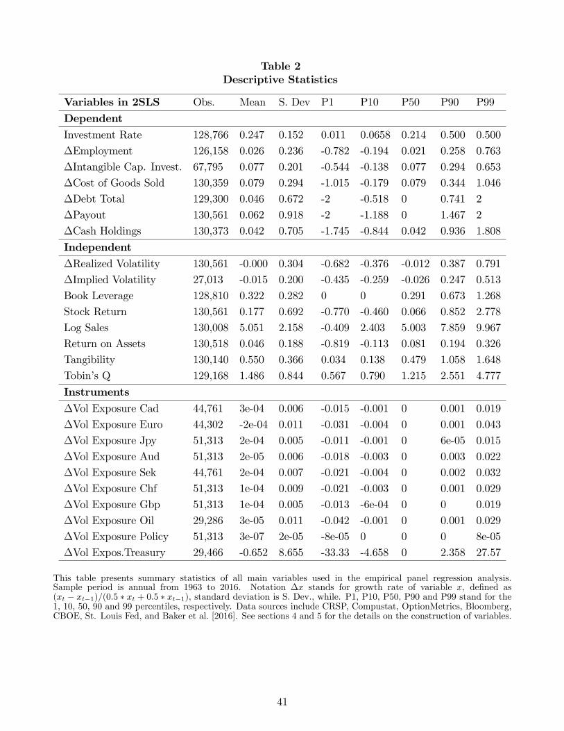
Table 2Descriptive Statistics

Variables in 2SLS Obs. Mean S. Dev P1 P10 P50 P90 P99

DependentInvestment Rate 128,766 0.247 0.152 0.011 0.0658 0.214 0.500 0.500

∆Employment 126,158 0.026 0.236 -0.782 -0.194 0.021 0.258 0.763

∆Intangible Cap. Invest. 67,795 0.077 0.201 -0.544 -0.138 0.077 0.294 0.653

∆Cost of Goods Sold 130,359 0.079 0.294 -1.015 -0.179 0.079 0.344 1.046

∆Debt Total 129,300 0.046 0.672 -2 -0.518 0 0.741 2

∆Payout 130,561 0.062 0.918 -2 -1.188 0 1.467 2

∆Cash Holdings 130,373 0.042 0.705 -1.745 -0.844 0.042 0.936 1.808

Independent∆Realized Volatility 130,561 -0.000 0.304 -0.682 -0.376 -0.012 0.387 0.791

∆Implied Volatility 27,013 -0.015 0.200 -0.435 -0.259 -0.026 0.247 0.513

Book Leverage 128,810 0.322 0.282 0 0 0.291 0.673 1.268

Stock Return 130,561 0.177 0.692 -0.770 -0.460 0.066 0.852 2.778

Log Sales 130,008 5.051 2.158 -0.409 2.403 5.003 7.859 9.967

Return on Assets 130,518 0.046 0.188 -0.819 -0.113 0.081 0.194 0.326

Tangibility 130,140 0.550 0.366 0.034 0.138 0.479 1.058 1.648

Tobin’s Q 129,168 1.486 0.844 0.567 0.790 1.215 2.551 4.777

Instruments∆Vol Exposure Cad 44,761 3e-04 0.006 -0.015 -0.001 0 0.001 0.019

∆Vol Exposure Euro 44,302 -2e-04 0.011 -0.031 -0.004 0 0.001 0.043

∆Vol Exposure Jpy 51,313 2e-04 0.005 -0.011 -0.001 0 6e-05 0.015

∆Vol Exposure Aud 51,313 2e-05 0.006 -0.018 -0.003 0 0.003 0.022

∆Vol Exposure Sek 44,761 2e-04 0.007 -0.021 -0.004 0 0.002 0.032

∆Vol Exposure Chf 51,313 1e-04 0.009 -0.021 -0.003 0 0.001 0.029

∆Vol Exposure Gbp 51,313 1e-04 0.005 -0.013 -6e-04 0 0 0.019

∆Vol Exposure Oil 29,286 3e-05 0.011 -0.042 -0.001 0 0.001 0.029

∆Vol Exposure Policy 51,313 3e-07 2e-05 -8e-05 0 0 0 8e-05

∆Vol Expos.Treasury 29,466 -0.652 8.655 -33.33 -4.658 0 2.358 27.57

This table presents summary statistics of all main variables used in the empirical panel regression analysis.Sample period is annual from 1963 to 2016. Notation ∆x stands for growth rate of variable x, defined as(xt − xt−1)/(0.5 ∗ xt + 0.5 ∗ xt−1), standard deviation is S. Dev., while. P1, P10, P50, P90 and P99 stand for the1, 10, 50, 90 and 99 percentiles, respectively. Data sources include CRSP, Compustat, OptionMetrics, Bloomberg,CBOE, St. Louis Fed, and Baker et al. [2016]. See sections 4 and 5 for the details on the construction of variables.

41

Table3

Parametervaluesunderbenchmarkcalibration

Description

Notation

Value

Justification

Technology

Subjectivediscountfactor

β0.988

Long-runaverageofU.S.firm-leveldiscountrate

Returnonsaving

r n0.01

80%oftherisk-freerate(thecashtoassetratioforcashholdingfirms)

Shareoncapital

α0.33

Capitalshareinoutputisone-third,laborshareistwo-thirds

Markup

ε4

33%markup.Withconstantreturnstoscaleyieldsa+b=075

Wage

w1

Wageratenormalizedto1

Rateofdepreciationforcapital

δ0.03

Capitaldepreciationrateassumed3%

permonth

Fixedcostofinvestment

c k0.01

1%ofquarterlyoutput(Wealsoshow

robustnesswith2%,4%)

Fixedoperatingcost

F0.2

Firms’averageSG&Atosalesratio

Uncertaintyshock(2stateMarkov)

Conditionalvolatilityofproductivity

σL

0.051

Baselineuncertainty(Bloom

etal2016)

Conditionalvolatilityinhighuncertaintystate

σH

0.209

Uncertaintyshocks4.1*baselineuncertainty(Bloom

etal2016)

Transitionprobabilitylowtohighuncertainty

πσ L,H

2.60%

Uncertaintyshocksexpectedevery9.6years(Bloom

etal2016)

Transitionprobabilityremaininginhighuncertainty

πσ H,H

94%

Quarterlyprobabilityofremaininginhighuncertainty(Bloom

etal2016)

Persistenceofloggedidiosyncraticproductivity

ρz

0.95

Quarterlypersistenceofidiosyncraticproductivity(Khan&Thomas2008)

Stochasticfinancingcost(2stateMarkov)

Low

externalfinancingcoststate

ηL

0.005

Low

financingcost.5%ofoutput(AltinkilicandHansen2000)

Highexternalfinancingcoststate

ηH

0.05

Highfinancingcost5%

ofoutput(Altinkilic&Hansen2000).Alsotried0.025&0.1

Transitionprobabilitylowtohighfinancingcoststate

πη L,H

2.60%

Sameasuncertaintyshock(Alsotried5%)

Transitionprob.remaininginhighfinancingcoststate

πη H,H

94%

Sameasuncertaintyshock(Alsotried50%)

Impactofuncertaintyonfinancialcost

λ0.03

CorrelationbetweentheBaa-AaaspreadandVIX

Thistablepresentsthepredeterminedandthecalibratedparametervaluesofthebenchmarkmodel.

42

Table 4Coeffi cient on changes in volatility for real and financial variables.

Real Financial

I/K dEmp dCash dDiv

A: Data∆Volatility -0.080 -0.068 0.197 -0.522

B: Real frictions∆Volatility -0.042 -0.014 0.000 -0.031

C: Financial frictions∆Volatility -0.021 -0.004 1.071 -0.700

D: Real+financial frictions∆Volatility -0.077 -0.027 0.316 -0.372

E: No frictions∆Volatility 0.003 0.006 0.000 -7.230

Row (A) Data reports the results for investment rate, employment growth, cash growth and equity payout growthfrom columns (2) of tables (5), (7) and (8) respectively. Rows (B) to (E) reports the model counterparts fromregressions using simulation data on lagged volatility (σ2

i,t). The reported statistics in the model are averages from100 samples of simulated data, each with 3000 firms and 200 quarterly observations. We report the cross-simulationaveraged annual moments. I/K is the investment rate, dEmp is the employment growth, dCash is the cash growthrate, and dDiv the dividend growth in the model and cash dividend plus repurchase growth in the data. Forcomparability all the regressions (in the data and model) include firm and time fixed effects and all are significantat the 1% level with firm-clustered standard errors. The only difference is employment is annual in the real data(since no quarterly real employment data is available).

43

Table 5Investment rate

(1) (2) (3) (4) (5) (6)

Investment ratei,t OLS IV IV OLS IV IV

Realized Realized Realized Implied Implied Implied

∆Volatilityi,t−1 -0.031*** -0.080*** -0.028*** -0.089*** -0.215*** -0.079**

(-19.896) (-3.881) (-2.754) (-10.520) (-4.220) (-2.584)

Book Leveragei,t−1 -0.050*** -0.037***

(-8.444) (-5.739)

Stock Returni,t−1 0.008*** 0.005*

(2.957) (1.747)

Log Salesi,t−1 -0.021*** -0.020***

(-6.673) (-5.013)

Return on Assetsi,t−1 0.129*** 0.120***

(5.188) (3.710)

Tangibilityi,t−1 -0.114*** -0.120***

(-5.953) (-3.366)

Tobin’s Qi,t−1 0.050*** 0.054***

(10.013) (8.330)

1st moment 10IVi,t−1 No No Yes No No Yes

Firm, time FE Yes Yes Yes Yes Yes Yes

SE cluster(3SIC) Yes Yes Yes Yes Yes Yes

Observations 127,361 28,650 28,326 26,237 17,683 17,487

F 1st st. Cragg-D 166.8 179.2 78.79 60.41

F 1st st. Kleib.-P 19.33 18.02 13.20 11.49

p-val Sargan—H J 0.246 0.873 0.680 0.988

This table presents OLS and 2SLS annual regression results of firm-level investment rate on 1-year lagged changesin firm-level volatility and lagged level of firm-level controls. Investment rate at fiscal year t is defined as It/Kt−1

(capex/lagged net property plant & equipment from Compustat). Sample period is from 1963 to 2016. Specifications1,2,4, and 5 are univariate, while 3 and 6 multivariate. Only 1 and 4 are OLS while all others 2SLS. The latterinstrument lagged changes in firm-level volatility with industry-level (3SIC) exposure to 10 aggregate laggeduncertainty shocks. These instruments include the lagged exposure to annual changes in expected volatility ofenergy, currencies, and 10-year treasuries (as proxied by at-the-money forward-looking implied volatilities of oil,7 widely traded currencies, and TYVIX) and lagged exposure to changes in economic policy uncertainty fromBaker et al. [2016]. We measure firm-level uncertainty in two ways: realized and implied volatility. Annual realizedvolatility is the 12-month standard deviation of daily stock returns from CRSP. We annualize this standard deviationby multiplying by the square root of 252 (average trading days in a year). Implied volatility is proxied by the annualaverage of each firm’s daily 365-day implied volatility of at-the-money-forward call options from OptionMetrics. Allregressors are lagged by 1-year. To ensure that the changes in both firm- and aggregate-level volatility are annualwe require a 12 month distance between each firm’s fiscal-year end dates, starting from t − 2 and ending in t. Inall specifications we include both firm and calendar-year fixed effects. Standard errors are clustered at the 3-digitSIC industry. Our main set of firm-level controls include the lagged level of book leverage, stock return, log sales,return on assets, tangibility, and Tobin’s Q. Moreover, to tease out the impact of 2nd moment uncertainty shockswe also include as controls the lagged exposure to changes in the return on each of the 10 aggregate instruments(i.e., 1st moment shocks). Data availability on implied volatility of treasuries and oil restrict the start of the 2SLSsample to fiscal year 2006. Statistical significance: *** p<0.01, ** p<0.05, * p<0.1, † p<0.15. t-statistics are inparentheses. See sections 4 and 5 for details on data. 44

Table 6Investment rate - 2SLS 1st Stage Results

Specification: Univariate Multivariate

Set-up: ∆Volatilityi,t−1 Realized Implied Realized Implied

∆Vol Exposure Cadi,t−1 3.975*** 1.516*** 3.700*** 1.304***

(5.07) (3.8) (4.93) (3.39)

∆Vol Exposure Euroi,t−1 1.259*** 0.611*** 1.154*** 0.458***

(4.22) (3.69) (4.05) (2.94)

∆Vol Exposure Jpyi,t−1 2.368*** 0.364 2.375*** 0.393

(3.98) (0.84) (4.01) (0.94)

∆Vol Exposure Audi,t−1 5.152*** 1.736*** 5.323*** 1.724***

(7.74) (5.85) (9.02) (5.94)

∆Vol Exposure Seki,t−1 4.308*** 1.320*** 4.848*** 1.557***

(7.72) (3.84) (7.57) (4.26)

∆Vol Exposure Chfi,t−1 2.120*** 1.255*** 2.403*** 1.353***

(6.14) (6.07) (6.3) (5.7)

∆Vol Exposure Gbpi,t−1 3.036*** 1.826*** 2.814*** 1.667***

(5.35) (4.33) (5.35) (4.65)

∆Vol Exposure Policyi,t−1 551.441*** 222.584* 561.499*** 172.483†(3.12) (1.93) (3.3) (1.64)

∆Vol Expos.Treasuryi,t−1‡ 3.079*** 1.099*** 3.036*** 0.933***

(8.52) (4.56) (8.57) (4.63)

∆Vol Exposure Oili,t−1 3.044*** 1.846*** 4.307*** 1.684***

(9.06) (7.71) (5.07) (5.1)

Observations 28,650 17,683 28,326 17,487

F-test 1st stage Cragg-Donald 166.8 78.79 179.2 60.41

F-test 1st stage Kleibergen-Paap 19.33 13.20 18.02 11.49

p-value Hansen-Sargan J 0.246 0.680 0.873 0.988

This table presents the 2SLS first stage regression results of firm-level investment rate on 1-year lagged changesin firm-level volatility and lagged level of firm-level controls. Columns 1 and 2 are the first stage results for theunivariate specifications (2) and (5) in Table 5, while columns 3 and 4 are the multivariate first stage resultsof specifications (3) and (6). We instrument lagged changes in firm-level volatility with industry-level (3SIC)exposure to 10 aggregate lagged uncertainty shocks. These instruments include the lagged exposure to annualchanges in expected volatility of energy, currencies, and 10-year treasuries (as proxied by at-the-money forward-looking implied volatilities of oil, 7 widely traded currencies, and TYVIX) and lagged exposure to changes ineconomic policy uncertainty from Baker et al. [2016]. We measure firm-level uncertainty in two ways: realized andimplied volatility. Annual realized volatility is the 12-month standard deviation of daily stock returns from CRSP.We annualize this standard deviation by multiplying by the square root of 252 (average trading days in a year).Implied volatility is proxied by the annual average of each firm’s daily 365-day implied volatility of at-the-money-forward call options from OptionMetrics. All regressors are lagged by 1-year. To ensure that the changes in bothfirm- and aggregate-level volatility are annual we require a 12 month distance between each firm’s fiscal-year enddates, starting from t− 2 and ending in t. In all specifications we include both firm and calendar-year fixed effects.Standard errors are clustered at the 3-digit SIC industry. Our main set of firm-level controls include the laggedlevel of book leverage, stock return, log sales, return on assets, tangibility, and Tobin’s Q. Moreover, to tease outthe impact of 2nd moment uncertainty shocks we also include as controls the lagged exposure to changes in thereturn on each of the 10 aggregate instruments (i.e., 1st moment shocks). Data availability on implied volatilityof treasuries and oil restrict the start of the 2SLS sample to fiscal year 2006. ‡ :The coeffi cients on treasuries arescaled upward by a factor of 1000 for presentational purposes. Statistical significance: *** p<0.01, ** p<0.05, *p<0.1, † p<0.15. t-statistics are in parentheses. See sections 4 and 5 for details on data.

45

Table 7Additional Real Quantities

(1) (2) (3) (4) (5) (6)

OLS IV IV OLS IV IV


A: ∆Intangible Capital Investmenti,t∆Volatilityi,t−1 -0.054*** -0.097*** -0.036** -0.138*** -0.187*** -0.056

(-10.848) (-4.134) (-2.208) (-9.347) (-2.869) (-1.066)

Observations 66,865 17,168 17,013 16,290 10,982 10,887

F 1st st. Cragg-D 109.6 111.9 41.06 38.04

F 1st st. Kleib.-P 15.10 16.33 8.325 10.30

p-val Sargan—H J 0.329 0.416 0.241 0.302

B: ∆Employmenti,t∆Volatilityi,t−1 -0.037*** -0.068*** -0.007 -0.115*** -0.241*** -0.045

(-11.867) (-2.657) (-0.248) (-10.677) (-3.429) (-0.550)

Observations 124,768 28,495 28,158 26,132 17,591 17,396

F 1st st. Cragg-D 165.9 178.1 79.12 60.25

F 1st st. Kleib.-P 18.92 17.59 13.36 11.66

p-val Sargan—H J 0.177 0.586 0.231 0.440

C: ∆Cost of Goods Soldi,t∆Volatilityi,t−1 -0.056*** -0.251** -0.137*** -0.209*** -0.807** -0.337***

(-10.376) (-2.241) (-3.642) (-5.642) (-2.436) (-3.086)

Observations 128,974 28,720 28,376 26,384 17,710 17,507

F 1st st. Cragg-D 167.6 179.8 78.98 60.42

F 1st st. Kleib.-P 19.24 17.94 13.18 11.50

p-val Sargan—H J 0.170 0.029 0.181 0.023

This table reports regression results of annual changes in intangible capital investment (research anddevelopment+selling, general and administrative expense from Compustat) (Panel A), changes in employment(Panel B), and changes in cost of goods sold (Panel C), where growth rates defined as (xt−xt−1)/(0.5∗xt+0.5∗xt−1).Specifications 1 through 6 follow the setup, timing, and set of controls included in the investment rate regressionin Table 5. To preserve space we do not report the coeffi cients and t-statistics on controls. The sample periodis annual from 1963 to 2016. Specifications 1,2,4, and 5 are univariate, while 3 and 6 multivariate. Only 1 and4 are OLS while all others 2SLS. The latter instrument lagged changes in firm-level volatility with industry-level(3SIC) exposure to 10 aggregate lagged uncertainty shocks. These instruments include the lagged exposure toannual changes in expected volatility of energy, currencies, and 10-year treasuries (as proxied by at-the-moneyforward-looking implied volatilities of oil, 7 widely traded currencies, and TYVIX) and lagged exposure to changesin economic policy uncertainty from Baker et al. [2016]. We measure firm-level uncertainty in two ways: realizedand implied volatility. Annual realized volatility is the 12-month standard deviation of daily stock returns fromCRSP. We annualize this standard deviation by multiplying by the square root of 252 (average trading days in ayear). Implied volatility is proxied by the annual average of each firm’s daily 365-day implied volatility of at-the-money-forward call options from OptionMetrics. All regressors are lagged by 1-year. To ensure that the changes inboth firm- and aggregate-level volatility are annual we require a 12 month distance between each firm’s fiscal-yearend dates, starting from t − 2 and ending in t. In all specifications we include both firm and calendar-year fixedeffects. Standard errors are clustered at the 3-digit SIC industry. Our main set of firm-level controls include thelagged level of book leverage, stock return, log sales, return on assets, tangibility, and Tobin’s Q. Moreover, to teaseout the impact of 2nd moment uncertainty shocks we also include as controls the lagged exposure to changes in thereturn on each of the 10 aggregate instruments (i.e., 1st moment shocks). Data availability on implied volatility oftreasuries and oil restrict the start of the 2SLS sample to fiscal year 2006. Statistical significance: *** p<0.01, **p<0.05, * p<0.1, † p<0.15. t-statistics are in parentheses. See sections 4 and 5 for details on data.

46

Table 8Financial Outcomes

(1) (2) (3) (4) (5) (6)OLS IV IV OLS IV IVRealized Realized Realized Implied Implied Implied

A: ∆Total Debti,t∆Volatilityi,t−1 -0.078*** -0.256*** -0.160** -0.198*** -0.811*** -0.678***

(-9.702) (-3.400) (-2.382) (-6.744) (-5.407) (-4.217)Observations 127,911 28,545 28,320 26,198 17,586 17,470F 1st st. Cragg-D 166.3 179.5 77.67 60.15F 1st st. Kleib.-P 19.10 17.85 13.14 11.52p-val Sargan—H J 0.0967 0.334 0.761 0.856B: ∆Payouti,t∆Volatilityi,t−1 -0.158*** -0.522*** -0.297*** -0.521*** -1.394*** -0.803**

(-13.318) (-4.772) (-2.710) (-8.548) (-4.743) (-2.590)Observations 129,158 28,738 28,389 26,402 17,715 17,512F 1st st. Cragg-D 167.6 180 78.97 60.41F 1st st. Kleib.-P 19.24 17.93 13.17 11.48p-val Sargan—H J 0.370 0.687 0.988 0.996C: ∆Cash holdingi,t∆Volatilityi,t−1 0.032*** 0.197*** 0.148** 0.115*** 0.639*** 0.516**

(3.714) (2.984) (2.253) (3.573) (3.850) (2.435)Observations 128,985 28,721 28,374 26,381 17,709 17,506F 1st st. Cragg-D 167.6 179.8 78.92 60.38F 1st st. Kleib.-P 19.25 17.93 13.17 11.50p-val Sargan—H J 0.664 0.559 0.441 0.511

This table reports regression results of annual changes in total debt (Panel A), changes in firm payout (cash dividend+ share repurchase) (Panel B), and changes in cash holdings (cash and short-term investments) (Panel C), wheregrowth rates are defined as (xt − xt−1)/(0.5 ∗ xt + 0.5 ∗ xt−1). Specifications 1 through 6 follow the setup, timing,and set of controls included in the investment rate regression in Table 5. To preserve space we do not report thecoeffi cients and t-statistics on controls. The sample period is annual from 1963 to 2016. Specifications 1,2,4, and 5are univariate, while 3 and 6 multivariate. Only 1 and 4 are OLS while all others 2SLS. The latter instrument laggedchanges in firm-level volatility with industry-level (3SIC) exposure to 10 aggregate lagged uncertainty shocks. Theseinstruments include the lagged exposure to annual changes in expected volatility of energy, currencies, and 10-yeartreasuries (as proxied by at-the-money forward-looking implied volatilities of oil, 7 widely traded currencies, andTYVIX) and lagged exposure to changes in economic policy uncertainty from Baker et al. [2016]. We measure firm-level uncertainty in two ways: realized and implied volatility. Annual realized volatility is the 12-month standarddeviation of daily stock returns from CRSP. We annualize this standard deviation by multiplying by the squareroot of 252 (average trading days in a year). Implied volatility is proxied by the annual average of each firm’s daily365-day implied volatility of at-the-money-forward call options from OptionMetrics. All regressors are lagged by1-year. To ensure that the changes in both firm- and aggregate-level volatility are annual we require a 12 monthdistance between each firm’s fiscal-year end dates, starting from t − 2 and ending in t. In all specifications weinclude both firm and calendar-year fixed effects. Standard errors are clustered at the 3-digit SIC industry. Ourmain set of firm-level controls include the lagged level of book leverage, stock return, log sales, return on assets,tangibility, and Tobin’s Q. Moreover, to tease out the impact of 2nd moment uncertainty shocks we also includeas controls the lagged exposure to changes in the return on each of the 10 aggregate instruments (i.e., 1st momentshocks). Data availability on implied volatility of treasuries and oil restrict the start of the 2SLS sample to fiscalyear 2006. Statistical significance: *** p<0.01, ** p<0.05, * p<0.1, † p<0.15. t-statistics are in parentheses. Seesections 4 and 5 for details on data.

47

Table9

ImpactofRealizedVolatilityon

InvestmentforFinanciallyConstrainedandUnconstrainedFirmsduringFinancial

Crisisandnon-CrisisYears

Crisisperiod:Jan-01-2008toDec-31-2009

2SLSwithfullsetofcontrols(1-8)

InvestmentRate t

(1)

(2)

(3)

(4)

(5)

(6)

(7)

(8)

FinancialConstraintMeasure

S&PRatings

Whited-Wu

Employees

Assets

Age

Size&Age

∆Volatilityi,t−

1(R

ealized)

-0.028***

-0.012

-0.010

-0.025**

-0.026**

-0.022**

-0.021**

-0.017†

Dcrisis,t

--

--

--

-

Dcrisis,t·∆Volatilityi,t−

1-0.087***

-0.070***

-0.063***

-0.068***

-0.102***

-0.059**

-0.092***

Dfin_constrained,i,t−

1-0.006*

0.006

0.005

0.002

--0.026


1·∆Volatilityi,t−

1-0.007

0.020†

0.019

0.017

0.006

0.016

Dcrisis,t·D

fin_constrained,i,t−

10.003

-0.012*

-0.012*

-0.018***

-0.000

-0.013**

Dcrisis,t·D



1-0.028

-0.047**

-0.053**

-0.039*

-0.021

-0.042*

Observations

28,326

28,326

28,326

21,345

21,203

21,315

22,380

21,353

F-test1ststageCragg-D

179.2

80.92

39.33

26.97

33.28

22.34

33.34

25.18

F-test1ststageKleib.-P.

18.02

8.550

5.495

4.249

4.793

5.224

4.745

5.810

p-valSargan—HansenJ

0.873

0.652

0.587

0.530

0.728

0.805

0.944

0.671

Thistablepresentstheimpactofexogenousfirm-levelrealizedvolatilityoninvestmentratesoffinanciallyconstrainedandunconstrainedfirmsduringfinancial

crisisandnon-crisisyears.Allregressionsare2SLSofinvestmentrate-observedatfiscalyeartanddefinedasI t/Kt−

1(capex/laggednetpropertyplant&

equipmentfrom

Compustat)-on1-yearlaggedchangesinfirm-levelrealizedvolatilityandafullsetoflaggedfirm-levelcontrols.Allspecificationsfollowthe

setup,timing,andcontrolsincludedinspecification(3)inTable5.Column1restatesthebenchmarkregression(3)inTable5.Column2furtheraddsthe

interactionoflaggedchangeinrealizedvolatilitywithafinancial-crisisdummyvariablethattakesvalue1forallfirm-fiscal-yearobservationsofinvestment

rateendinginbetweenJan.12008andDec.312009,zerootherwise.Thisperiodcomprisesthecoremonthsofthegreatrecessioninwhichfirmswouldhave

observedatleast6monthsofheightenedfinancialfrictionsintheirannualaccountingreports.Columns3to8runadifference-in-difference-in-difference

specificationwherewefurtherinteractlaggedchangesinvolatilitywithstandardmeasuresoffinancialconstraintsandthecrisisdummy.Inparticular,using

eachfirm’sfinancialconstraintindexateveryfiscalyeart−

1weclassifyfirmsintoconstrainedandunconstrainedgroupsusingthe40and60percentile

cutoffsobtainedfrom

thecross-sectionalfiscal-yeardistributionoftheunderlyingfinancialconstraintindex.Weconsiderafirmconstrainedifitst−

1index

valueisequaltoorgreaterthanthe60percentileandunconstrainedifequaltoorlessthanthe40percentile.Weexcludefirm-timeobservationsinthe

middle50+/-10percentilestoincreaseprecisionintheclassificationoffirms.WedothisinallbuttheS&Pcredit-ratingfinancialconstraintmeasure.Here

wefollowDuchinetal.[2010]andconsiderafirmconstrainedifithaspositivedebtandnobondratingandunconstrainedotherwise(whichincludesfirms

withzerodebtandnodebtrating).Theother5measuresoffinancialconstraintsareconstructedusingtheWhited-Wuindex,reciprocalofemployees,

reciprocaloftotalassets,reciprocalofageinwhichageisdefinedasthenumberofyearssincefirmincorporation,andtheSA

indexbasedonsizeandage

ofHadlockandPierce[2010].WethankToniWhitedforsuggestingthislastindex.Inallspecificationsweincludebothfirmandcalendar-yearfixedeffects.

Standarderrorsareclusteredatthe3digitSICindustry.Ourmainsetoffirm-levelcontrolsincludethelaggedlevelofbookleverage,stockreturn,logsales,

returnonassets,tangibility,andTobin’sQ.Moreover,toteaseouttheimpactof2ndmomentuncertaintyshockswealsoincludeascontrolsthelagged

exposuretochangesinthereturnoneachofthe10aggregateinstruments(i.e.,1stmomentshocks).Dataavailabilityonimpliedvolatilityoftreasuriesand

oilrestrictthestartofthe2SLSsampletofiscalyear2006.Statisticalsignificance:***p<0.01,**p<0.05,*p<0.1,†p<0.15.t-statisticsareinparentheses.

Seesections4and5fordetailsondata.

48

Table A1Coeffi cient on changes in volatility for real and financial variables.

High financial state/low financial sate Real Financial

I/K dEmp dCash dDiv

A: Benchmark∆Volatility -0.077 -0.027 0.316 -0.372

B: H/L = 5∆Volatility -0.085 -0.029 0.263 -0.322

C: Different transition matrix of ηt∆Volatility -0.079 -0.027 0.245 -0.399

D: Model with debt and equity∆Volatility -0.078 -0.028 0.141 -0.511

This table reports the model regression results of real and financial variables on volatility growth. The reportedstatistics in the model are averages from 100 samples of simulated data, each with 3000 firms and 200 quarterlyobservations. We report the cross-simulation averaged annual moments. I/K is the investment rate, dEmp is theemployment growth, dCash is the cash growth rate, and dDiv the dividend growth in the model and cash dividendplus repurchase growth in the data. Panel A is the benchmark calibration with this ratio equal to 10. Panels Blowers the high financing-cost-state-to-low-cost-state ratio (ηH/ηL ) to 5 while keeping the low financial cost stateηL = 0.005. Panel E sets the transition probabilities of financial shocks of πσL,H = 0.05 and πσH,H = 0.5. Panel Dextends the benchmark by including collateralized debt. All the regressions include firm and time fixed effects andall results for the model are significant at the 1% level with firm-clustered standard errors.

49

TableA2

2SLSSensitivitytoIndividualInstruments

(1)

(2)

(3)

(4)

(5)

(6)

(7)

(8)

(9)

(10)

IVDropped

None

Cad

Euro

Jpy

Aud

Sek

Chf

Gbp

Policy

Oil+Treasuries

RealVariables

InvestmentRate i,t

-0.028***

-0.031***

-0.026**

-0.028***

-0.031***

-0.031**

-0.028**

-0.027**

-0.028***

-0.033**

∆Intang.Cap.Invest. i,t

-0.036**

-0.036**

-0.035*

-0.039**

-0.038**

-0.031*

-0.042**

-0.041**

-0.034**

-0.039*

∆Employment i,t

-0.007

-0.004

-0.004

-0.007

-0.005

-0.031

-0.013

-0.007

-0.006

0.011

FinancialVariables

∆DebtTotali,t

-0.160**

-0.154**

-0.145**

-0.160**

-0.198***

-0.196***

-0.158**

-0.157**

-0.163**

-0.196**

∆Payout i,t

-0.297***

-0.320***

-0.286***

-0.293***

-0.364***

-0.279**

-0.254**

-0.288**

-0.289***

-0.444***

∆CashHoldings i,t

0.148**

0.141**

0.148**

0.144**

0.182**

0.151*

0.103†

0.140**

0.143**

0.254**

1stmoment10IV

i,t−

1Yes

Yes

Yes

Yes

Yes

Yes

Yes

Yes

Yes

Yes

Firm,timeFE

Yes

Yes

Yes

Yes

Yes

Yes

Yes

Yes

Yes

Yes

SEcluster(3SIC)

Yes

Yes

Yes

Yes

Yes

Yes

Yes

Yes

Yes

Yes

InvestmentRateStats

Observations

28,326

28,326

28,326

28,326

28,326

28,326

28,326

28,326

28,326

42,732

F1ststageCragg-D

179.2

185.2

191.4

195.6

169.2

158.5

179.9

190.3

193.9

105.2

F1ststageKleib.-P.

18.02

20.35

2018.49

14.91

18.71

18.50

16.92

19.05

13.34

p-valSargan—HansJ

0.873

0.935

0.865

0.813

0.857

0.846

0.806

0.864

0.808

0.972

Thistablepresents2SLSmultivariateregression

resultsforallourmainrealandfinancialoutcomevariables(withfullsetofcontrols)whenwedrop

individualinstrumentsoneatatimefrom

ourbenchmarksetof10instrumentalvariables(IVs).Inthelastcolumn(10)wedropbothoilandtreasuryIVs

astheseconstrainthestartofthesampletofiscalyear2006,whereaskeepingonlycurrenciesandpolicyIVsallowanadditional4yearsofpaneldata-with

firstfiscalyearofdependentvariablestartingin2002.SampleperiodendsinDecember2016.Thecoefficientandstatisticsreportedin(1)arefrom

the

benchmark2SLSmultivariateregressiononlaggedfirm-levelrealizedvolatilityshockspresentedincolumn(3)acrossTables5,7,and8.Thestatisticsunder

"InvestmentRateStats"correspondtothe1ststageresultsofthemultivariate2SLSregressionofinvestmentrateonlaggedchangeinrealizedvolatility

andmainsetoflaggedlevelcontrols.1stStagestatisticsforotherrealandfinancialestimationsarelargelycomparabletotheirbenchmarkspecifications

withthefullsetofinstruments.Inallspecificationsweincludebothfirmandcalendar-yearfixedeffects.Standarderrorsareclusteredatthe3digitSIC

industry.Ourmainsetoffirm-levelcontrolsincludethelaggedlevelofbookleverage,stockreturn,logsales,returnonassets,tangibility,andTobin’s

Q.Moreover,toteaseouttheimpactof2ndmomentuncertaintyshockswealsoincludeascontrolsthelaggedexposuretothereturnoneachofthe10

aggregateinstruments(i.e.,1stmomentshocks).Dataavailabilityonimpliedvolatilityoftreasuriesandoilrestrictthestartofthe2SLSsampletofiscal

year2006.Statisticalsignificance:***p<0.01,**p<0.05,*p<0.1,†p<0.15.t-statisticsareinparentheses.Seesections4and5fordetailsondata.

50

TableA3

2SLSRobustnessTests

(1)

(2)

(3)

(4)

(5)

(1A)

(2A)

(3A)

(4A)

(5A)

VolatilityInstrumented

Realized

Realized

Realized

Realized

Realized

Implied

Implied

Implied

Implied

Implied

RealVariables

InvestmentRate i,t

-0.028***

-0.028***

-0.028***

-0.028***

-0.028***

-0.079**

-0.077***

-0.083**

-0.082***

-0.083***

∆IntangibleCap.Invest. i,t

-0.036**

-0.034**

-0.032**

-0.035**

-0.029*

-0.056

-0.049

-0.057

-0.049

-0.041

∆Employment i,t

-0.007

-0.006

-0.010

-0.008

-0.008

-0.045

-0.042

-0.048

-0.048

-0.044

FinancialVariables

∆DebtTotali,t

-0.160**

-0.159**

-0.166**

-0.161**

-0.165**

-0.678***

-0.662***

-0.685***

-0.681***

-0.670***

∆Payout i,t

-0.297***

-0.280***

-0.320***

-0.299***

-0.306***

-0.803**

-0.746**

-0.862***

-0.803**

-0.808***

∆CashHoldings i,t

0.148**

0.142**

0.138**

0.148**

0.137**

0.516**

0.514**

0.539***

0.517**

0.541***

Mainfirm-levelcontrolsi,t−

1Yes

Yes

Yes

Yes

Yes

Yes

Yes

Yes

Yes

Yes

Covariancew/market i,t−

1Yes

Yes

Yes

Yes

Financialconstraintindexes i,t−

1Yes

Yes

Yes

Yes

S&Pcreditratings i,t−

1Yes

Yes

Yes

Yes

1stmomentcontrols10IV

i,t−

1Yes

Yes

Yes

Yes

Yes

Yes

Yes

Yes

Yes

Yes

Firm,timeFE

Yes

Yes

Yes

Yes

Yes

Yes

Yes

Yes

Yes

Yes

SEclustering(3SICindustry)

Yes

Yes

Yes

Yes

Yes

Yes

Yes

Yes

Yes

Yes

InvestmentRateStats

Observations

28,326

28,326

28,148

28,326

28,148

17,487

17,487

17,391

17,487

17,391

F1ststageCragg-DonaldWald

179.2

191.5

178

179.1

190.3

60.41

67.22

6060.99

67.45

F1ststageKleibergen-PaapWald

18.02

2017.88

18.06

19.84

11.49

13.61

11.83

11.68

13.96

p-valSargan—HansenJChi-sq

0.873

0.873

0.824

0.858

0.806

0.988

0.988

0.970

0.987

0.964

Thistablepresents2SLSrobustnessresultsforallourrealandfinancialoutcomevariablesexaminedinmainTables5,7,and8.Columns(1)and(1A)

restateherethebenchmark2SLSspecificationsincolumns(3)and(6)ineachoftheirmainrespectiveTables.Thecontrolcovariancew/marketaddseach

firm’slaggedCAPMbetainthefullsetofcontrols.Thefinancialconstraintindexcolumnaddsasetof6laggedfirm-levelcontrolswhichproxyforfirm

financialconstraints.TheseincludethelaggedWhited-Wuindex,laggedSA

indexofHadlockandPierce(2010),theKaplan-Zingalesindex,reciprocalof

totalassets,reciprocalofemployees,andreciprocalofage-whereageisthenumberofyearssincefirmincorporation.TheS&Pcreditratingscolumnfurther

addsafullsetofdummiesbasedoneverypossiblecreditratingcategorygivenbyS&Ponlong-termdebt.Theomitteddummyisfornocreditratings.In

allspecificationsweincludebothfirmandcalendar-yearfixedeffects.Standarderrorsareclusteredatthe3-digitSICindustry.Statisticalsignificance:***

p<0.01,**p<0.05,*p<0.1,†p<0.15.t-statisticsareinparentheses.Seesections4and5forthedetailsontheconstructionofvariablesanddata.

51

Table A4Investment rate, Using Same Panel Across Specifications

(1) (2) (3) (4) (5) (6)

Investment ratei,t OLS IV IV OLS IV IV


∆Volatilityi,t−1 -0.033*** -0.081*** -0.029** -0.079*** -0.216*** -0.079**

(-4.572) (-3.531) (-2.550) (-7.374) (-4.174) (-2.584)

Book Leveragei,t−1 -0.040*** -0.037***

(-6.333) (-5.739)

Stock Returni,t−1 0.006** 0.005*

(2.156) (1.747)

Log Salesi,t−1 -0.021*** -0.020***

(-5.100) (-5.013)

Return on Assetsi,t−1 0.126*** 0.120***

(3.850) (3.710)

Tangibilityi,t−1 -0.124*** -0.120***

(-3.492) (-3.366)

Tobin’s Qi,t−1 0.056*** 0.054***

(8.176) (8.330)

1st moment 10IVi,t−1 No No Yes No No Yes

Firm, time FE Yes Yes Yes Yes Yes Yes

SE cluster(3SIC) Yes Yes Yes Yes Yes Yes

Observations 17,487 17,487 17,487 17,487 17,487 17,487

F 1st st. Cragg-D 137.4 145.8 78.34 60.41

F 1st st. Kleib.-P 16.03 15.44 13.16 11.49

p-val Sargan—H J 0.645 0.964 0.699 0.988

This table presents all investment rate regression results shown in main Table 5 but holding the sample of firm-timeobservations fixed across specifications. The sample is restricted to firms that have both non-missing lagged realizedand implied volatilities every fiscal year. The Table presents OLS and 2SLS annual regression results of firm-levelinvestment rate on 1-year lagged changes in firm-level volatility and lagged level of firm-level controls. Investmentrate at fiscal year t is defined as It/Kt−1 (capex/lagged net property plant & equipment from Compustat). Sampleperiod is from 1963 to 2016. Specifications 1,2,4, and 5 are univariate, while 3 and 6 multivariate. Only 1 and4 are OLS while all others 2SLS. The latter instrument lagged changes in firm-level volatility with industry-level(3SIC) exposure to 10 aggregate lagged uncertainty shocks. These instruments include the lagged exposure toannual changes in expected volatility of energy, currencies, and 10-year treasuries (as proxied by at-the-moneyforward-looking implied volatilities of oil, 7 widely traded currencies, and TYVIX) and lagged exposure to changesin economic policy uncertainty from Baker et al. [2016]. We measure firm-level uncertainty in two ways: realizedand implied volatility. Annual realized volatility is the 12-month standard deviation of daily stock returns fromCRSP. We annualize this standard deviation by multiplying by the square root of 252 (average trading days in ayear). Implied volatility is proxied by the annual average of each firm’s daily 365-day implied volatility of at-the-money-forward call options from OptionMetrics. All regressors are lagged by 1-year. To ensure that the changes inboth firm- and aggregate-level volatility are annual we require a 12 month distance between each firm’s fiscal-yearend dates, starting from t − 2 and ending in t. In all specifications we include both firm and calendar-year fixedeffects. Standard errors are clustered at the 3-digit SIC industry. Our main set of firm-level controls include thelagged level of book leverage, stock return, log sales, return on assets, tangibility, and Tobin’s Q. Moreover, to teaseout the impact of 2nd moment uncertainty shocks we also include as controls the lagged exposure to changes in thereturn on each of the 10 aggregate instruments (i.e., 1st moment shocks). Data availability on implied volatility oftreasuries and oil restrict the start of the 2SLS sample to fiscal year 2006. Statistical significance: *** p<0.01, **p<0.05, * p<0.1, † p<0.15. t-statistics are in parentheses. See sections 4 and 5 for details on data.

52

TableA5

ImpactofImplied

Volatilityon

InvestmentforFinanciallyConstrained

andUnconstrained

FirmsduringFinancial

Crisisandnon-CrisisYears

Crisisperiod:Jan-01-2008toDec-31-2009

2SLSwithfullsetofcontrols(1-8)

InvestmentRate t

(1)

(2)

(3)

(4)

(5)

(6)

(7)

(8)

FinancialConstraintMeasure

S&PRatings

Whited-Wu

Employees

Assets

Age

Size&Age

∆Volatilityi,t−

1(Implied)

-0.079**

-0.045†

-0.032

-0.059**

-0.084***

-0.055**

-0.058*

-0.065**

Dcrisis,t

--

--

--

-

Dcrisis,t·∆Volatilityi,t−

1-0.062***

-0.056**

-0.053**

-0.035

-0.083***

-0.053*

-0.049*


1-0.006

0.002

0.038*

0.019

--0.148***



1-0.018†

0.048**

0.041†

0.036

0.010

0.039**

Dcrisis,t·D


10.006

-0.001

-0.007

-0.013

0.000

-0.015*

Dcrisis,t·D



1-0.006

-0.093***

-0.093***

-0.069**

-0.019

-0.065**

Observations

17,487

17,487

17,487

13,084

13,306

13,050

13,943

12,910

F-test1ststageCragg-D

60.41

31.99

15.52

15.48

15.52

15.64

13.64

15.45

F-test1ststageKleib.-P.

11.49

10.95

8.055

7.678

10.69

6.265

5.141

7.736

p-valSargan—HansenJ

0.988

0.999

0.998

0.809

0.891

0.565

0.907

0.208

Thistablepresentstheimpactofexogenousfirm-levelimpliedvolatilityoninvestmentratesoffinanciallyconstrainedandunconstrainedfirmsduringfinancial

crisisandnon-crisisyears.Allregressionsare2SLSofinvestmentrate-observedatfiscalyeartanddefinedasI t/Kt−

1(capex/laggednetpropertyplant&

equipmentfrom

Compustat)-on1-yearlaggedchangesinfirm-levelimpliedvolatilityandafullsetoflaggedfirm-levelcontrols.Allspecificationsfollowthe

setup,timing,andcontrolsincludedinspecification(6)inTable5.Column1restatesthebenchmarkregression(6)inTable5.Column2furtheraddsthe

interactionoflaggedchangeinimpliedvolatilitywithafinancial-crisisdummyvariablethattakesvalue1forallfirm-fiscal-yearobservationsofinvestment

rateendinginbetweenJan.12008andDec.312009,zerootherwise.Thisperiodcomprisesthecoremonthsofthegreatrecessioninwhichfirmswouldhave

observedatleast6monthsofheightenedfinancialfrictionsintheirannualaccountingreports.Columns3to8runadifference-in-difference-in-difference

specificationwherewefurtherinteractlaggedchangesinvolatilitywithstandardmeasuresoffinancialconstraintsandthecrisisdummy.Inparticular,using

eachfirm’sfinancialconstraintindexateveryfiscalyeart−

1weclassifyfirmsintoconstrainedandunconstrainedgroupsusingthe40and60percentile

cutoffsobtainedfrom

thecross-sectionalfiscal-yeardistributionoftheunderlyingfinancialconstraintindex.Weconsiderafirmconstrainedifitst−

1index

valueisequaltoorgreaterthanthe60percentileandunconstrainedifequaltoorlessthanthe40percentile.Weexcludefirm-timeobservationsinthe

middle50+/-10percentilestoincreaseprecisionintheclassificationoffirms.WedothisinallbuttheS&Pcredit-ratingfinancialconstraintmeasure.Here

wefollowDuchinetal.[2010]andconsiderafirmconstrainedifithaspositivedebtandnobondratingandunconstrainedotherwise(whichincludesfirms

withzerodebtandnodebtrating).Theother5measuresoffinancialconstraintsareconstructedusingtheWhited-Wuindex,reciprocalofemployees,

reciprocaloftotalassets,reciprocalofageinwhichageisdefinedasthenumberofyearssincefirmincorporation,andtheSA

indexbasedonsizeandage

ofHadlockandPierce[2010].WethankToniWhitedforsuggestingthislastindex.Inallspecificationsweincludebothfirmandcalendar-yearfixedeffects.

Standarderrorsareclusteredatthe3digitSICindustry.Ourmainsetoffirm-levelcontrolsincludethelaggedlevelofbookleverage,stockreturn,logsales,

returnonassets,tangibility,andTobin’sQ.Moreover,toteaseouttheimpactof2ndmomentuncertaintyshockswealsoincludeascontrolsthelagged

exposuretochangesinthereturnoneachofthe10aggregateinstruments(i.e.,1stmomentshocks).Dataavailabilityonimpliedvolatilityoftreasuriesand

oilrestrictthestartofthe2SLSsampletofiscalyear2006.Statisticalsignificance:***p<0.01,**p<0.05,*p<0.1,†p<0.15.t-statisticsareinparentheses.

Seesections4and5fordetailsondata.

53

Figu

re 1

: Unc

erta

inty

, rea

l out

com

es a

nd fi

nanc

ial f

low

s

Not

es:

Inve

stm

ent

rate

from

inve

stm

ent

and

capi

tal

data

from

BEA

NIP

Sta

bles

.Em

ploy

men

tse

ason

ally

adju

sted

tota

lpr

ivat

eem

ploy

men

t,BL

SID

CES

0500

0000

25.S

hort-

term

debt

,lon

g-te

rmde

bt,a

ndca

shfro

mth

eN

IPA

Inte

grat

edM

acro

econ

omic

Acco

unts

Tabl

eS.

5.q

nonf

inan

cial

corp

orat

ebu

sine

ss,

defla

ted

byth

eC

PI(N

IPA

tabl

e1.

1.4,

line

1).S

hort-

term

debt

sum

ofop

enm

arke

tpap

er(li

ne12

3)an

dsh

ort-t

erm

loan

s(li

ne12

7).L

ong-

term

debt

sum

ofbo

nds

(line

125)

and

mor

tgag

es(li

ne13

0).C

ash

sum

ofcu

rrenc

yan

dtra

nsfe

rabl

ede

posi

ts(li

ne97

)an

dtim

ean

dsa

ving

sde

posi

ts(li

ne98

).Ag

greg

ate

real

divi

dend

from

Shille

r'sw

ebpa

geht

tp://

ww

w.e

con.

yale

.edu

/~sh

iller/d

ata.

htm

.Gro

wth

rate

sof

varia

bles

mov

ing

aver

age

with

aw

indo

wof

4qu

arte

rsah

ead.

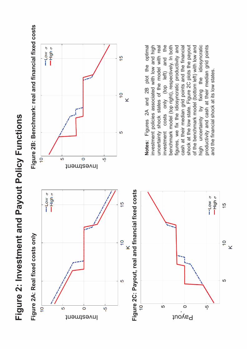
Figu

re 2

: Inv

estm

ent a

nd P

ayou

t Pol

icy

Func

tions

Not

es:

Figu

res

2Aan

d2B

plot

the

optim

alin

vest

men

tpo

licie

sas

soci

ated

with

low

and

high

unce

rtain

tysh

ock

stat

esof

the

mod

elw

ithre

alin

vest

men

tco

sts

only

(top

left)

and

the

benc

hmar

km

odel

(top

right

),re

spec

tivel

y.In

both

figur

es,

we

fixth

eid

iosy

ncra

ticpr

oduc

tivity

and

cash

atth

eir

med

ian

grid

poin

tsan

dth

efin

anci

alsh

ock

atth

elo

wst

ate.

Figu

re2C

plot

sth

epa

yout

ofth

ebe

nchm

ark

mod

el(b

otto

mle

ft)w

ithlo

wan

dhi

ghun

certa

inty

byfix

ing

the

idio

sync

ratic

prod

uctiv

ityan

dca

shat

thei

rm

edia

ngr

idpo

ints

and

the

finan

cial

shoc

kat

itslo

wst

ates

.

Figu

re2A

:Rea

lfix

edco

sts

only

Figu

re2B

:Ben

chm

ark:

real

and

finan

cial

fixed

cost

s

Figu

re2C

:Pay

out,

real

and

finan

cial

fixed

cost

s

Investment

Investment

Payout

Figu

re3:

The

Impa

ctof

apu

reU

ncer

tain

tySh

ock

Not

es:W

epl

otth

epe

rcen

tdev

iatio

nsof

aver

age

capi

tal,

labo

r,ou

tput

,cas

h,in

vest

men

t,an

dag

greg

ate

TFP

from

thei

rva

lues

inqu

arte

r0

ofth

ree

mod

elsp

ecifi

catio

ns:i

)th

em

odel

with

real

cost

only

(bla

ckx-

mar

k);i

i)th

em

odel

with

finan

cial

cost

only

(blu

eci

rcle

),an

diii)

the

benc

hmar

kw

ithbo

thre

alan

dfin

anci

alco

sts

(red

trian

gle)

.All

plot

sar

eba

sed

onsi

mul

atio

nsof

30,0

00fir

ms

of10

00-q

uarte

rlen

gth.

We

impo

sean

unce

rtain

tysh

ock

inth

equ

arte

rlab

elle

d1,

allo

win

gno

rmal

evol

utio

nof

the

econ

omy

afte

rwar

ds.

Figu

re4:

The

Impa

ctof

apu

reFi

nanc

ialS

hock

Not

es:W

epl

otth

epe

rcen

tdev

iatio

nsof

aver

age

capi

tal,

labo

r,ou

tput

,cas

h,in

vest

men

t,an

dag

greg

ate

TFP

from

thei

rva

lues

inqu

arte

r0

ofth

ree

mod

elsp

ecifi

catio

ns:i

)th

em

odel

with

real

cost

only

(bla

ckx-

mar

k);i

i)th

em

odel

with

finan

cial

cost

only

(blu

eci

rcle

),an

diii)

the

benc

hmar

kw

ithbo

thre

alan

dfin

anci

alco

sts

(red

trian

gle)

.All

plot

sar

eba

sed

onsi

mul

atio

nsof

30,0

00fir

ms

of10

00-q

uarte

rlen

gth.

We

impo

sea

finan

cial

shoc

kin

the

quar

terl

abel

led

1,al

low

ing

norm

alev

olut

ion

ofth

eec

onom

yaf

terw

ards

.

Figu

re 5

: The

Impa

ct o

f Unc

erta

inty

and

Fin

anci

al S

hock

s

Not

es:W

epl

otth

epe

rcen

tdev

iatio

nsof

aver

age

capi

tal,

labo

r,ou

tput

,cas

h,in

vest

men

t,an

dag

greg

ate

TFP

from

thei

rval

ues

inqu

arte

r0

ofth

ebe

nchm

ark

mod

elw

ithbo

thre

alan

dfin

anci

alco

sts.

Allp

lots

are

base

don

sim

ulat

ions

of30

,000

firm

sof

1000

-qu

arte

rle

ngth

.W

eim

pose

anun

certa

inty

shoc

k(b

lack

x-m

ark)

,a

finan

cial

shoc

k(b

lue

circ

le)

and

aco

mbi

ned

unce

rtain

tyan

dfin

anci

alsh

ocks

(red

trian

gle)

inth

equ

arte

rlab

elle

d1,

allo

win

gno

rmal

evol

utio

nof

the

econ

omy

afte

rwar

ds.

Figu

re 6

: Inv

estm

ent b

y m

ore

and

less

fina

ncia

lly c

onst

rain

ed fi

rms

Not

es:P

lots

the

inve

stm

entr

ate

forf

inan

cial

lym

ore-

cons

train

edfir

ms

(red

line,

diam

ond

mar

kers

)and

less

-con

stra

ined

firm

s(b

lue

line,

circ

lem

arke

rs)

agai

nstt

hele

ftax

is.F

inan

cial

cons

train

tsde

fined

asa

firm

havi

ngsh

orto

rlo

ngte

rmde

btbu

tno

bond

ratin

g(s

eeD

uchi

n,O

zbas

and

Sens

oy,

JFE

2010

and

Faul

kend

eran

dPe

ters

en,

RFS

2006

).St

ock-

mar

ket

vola

tility

(gre

enlin

e,no

-m

arke

rs)p

lots

daily

S&P5

00vo

latil

ityby

year

,rig

htax

is.

Investment rate (normed to 2006Q1=0)Stock market volatility

Less

con

stra

ined

Mor

e co

nstra

ined

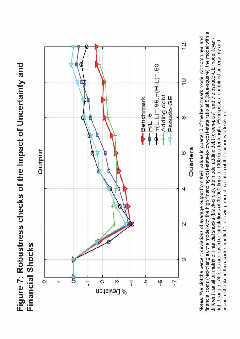
Figu

re 7

: Rob

ustn

ess

chec

ks o

f the

Impa

ct o

f Unc

erta

inty

and

Fi

nanc

ial S

hock

s

Not

es: W

e pl

ot th

e pe

rcen

t dev

iatio

ns o

f ave

rage

out

put f

rom

thei

r val

ues

in q

uarte

r 0 o

f the

ben

chm

ark

mod

el w

ith b

oth

real

and

fin

anci

al c

osts

(red

-tria

ngle

), th

e m

odel

with

the

high

fina

ncin

g-co

st-s

tate

-to-lo

w-c

ost-s

tate

ratio

at 5

(blu

e-sq

uare

), th

e m

odel

with

a

diffe

rent

tran

sitio

n m

atrix

of f

inan

cial

sho

cks

(bla

ck-c

ircle

), th

e m

odel

add

ing

debt

(gre

en-p

lus)

, and

the

pseu

do-G

E m

odel

(cya

n-rig

ht tr

iang

le).

All p

lots

are

bas

ed o

n si

mul

atio

ns o

f 30,

000

firm

s of

100

0-qu

arte

r len

gth.

We

impo

se a

com

bine

d un

certa

inty

and

finan

cial

sho

cks

in th

e qu

arte

r lab

elle

d 1,

allo

win

g no

rmal

evo

lutio

n of

the

econ

omy

afte

rwar

ds.

the finance uncertainty multiplier

Documents