THE FIELD-PROGRAMMABLE GATE ARRAY DESIGN OF THE GRIDDED

RETARDING ION DISTRIBUTION SENSOR

by

Anthony P. Swenson

A thesis submitted in partial fulfillmentof the requirements for the degree

of

MASTER OF SCIENCE

in

Electrical Engineering

Approved:

Ryan Davidson, Ph.D. Alan Marchant, Ph.D.Major Professor Committee Member

Jacob Gunther, Ph.D. Mark R. McLellan, Ph.D.Committee Member Vice President for Research and

Dean of the School of Graduate Studies

UTAH STATE UNIVERSITYLogan, Utah

2017

ii

Copyright c© Anthony P. Swenson 2017

All Rights Reserved

iii

ABSTRACT

The Field-Programmable Gate Array Design of the Gridded Retarding Ion Distribution

Sensor

by

Anthony P. Swenson, Master of Science

Utah State University, 2017

Major Professor: Ryan Davidson, Ph.D.Department: Electrical and Computer Engineering

This thesis project is concerned with two instruments that are used to measure plasma

in the low-Earth orbit space environment. These two instruments are the Retarding Po-

tential Analyzer (RPA), and the Ion Drift Meter (IDM). Work has been done to combine

the functionality from both of these instruments into one unit suitable for a small satellite

in terms of size, power, and mass. An electrical and mechanical design has already been

completed to this end and this new instrument is called the Gridded Retarding Ion Distri-

bution Sensor (GRIDS). The focus of this thesis is completing a field-programmable gate

array (FPGA) design for this instrument.

This document presents the design of the FPGA code along with the testing of that

code. The design includes two modes of operation, referred to as the 50/50 mode and the

10 Hz mode. Also, descriptions of various systems critical to proper instrument function,

such as the data output system and instrument ranging system, are included. Testing shows

that the instrument performs as desired.

(50 pages)

iv

PUBLIC ABSTRACT

The Field-Programmable Gate Array Design of the Gridded Retarding Ion Distribution

Sensor

Anthony P. Swenson

Mankind’s ability to predict weather on earth has been greatly enhanced by new instru-

mentation technology. Similarly, mankind’s ability to predict space weather benefits from

new technologies. Just as increasing the amount of atmospheric measurements on earth

heightened mankind’s ability to predict Earth weather, many scientists expect that ex-

panding the amount of plasma measurements in space could be key to enhancing mankind’s

ability to predict space weather. Small satellites are one of these new technologies that

have the potential to greatly enhance our ability to predict space weather. Utilizing many

low-cost small satellites allows scientists to take data from more locations than possible

with a few high-cost large satellites.

Two instruments that have historic use measuring plasma are the Retarding Potential

Analyzer and the Ion Drift Meter. Previous work has been done to combine the functionality

from both of these instruments into one unit suitable for a small satellite in terms of size,

power, and mass. An electrical and mechanical design has been completed to this end and

this new instrument is called the Gridded Retarding Ion Distribution Sensor. This thesis

describes the design and testing of the FPGA code that runs this new instrument.

v

ACKNOWLEDGMENTS

My major professor, Dr. Ryan Davidson, has been incredibly helpful and patient

through the whole process of my working on this thesis. His professionalism and work ethic

are qualities I hope to emulate one day. I couldn’t ask for a better Major Professor to work

with.

The faculty of Utah State University’s Electrical and Computer Engineering depart-

ment deserve many thanks for their tutoring and enthusiasm for teaching. Without these

professors I wouldn’t have near the knowledge and engineering ability that I have now.

I’d also like to thank my father, Dr. Charles Swenson, as I wouldn’t have pursued a

masters thesis without his influence.

I would like to thank my wife Emma for all of her love and support. Her along with

my family and friends helped me stay sane and motivated through the long and arduous

process of completing this thesis.

Anthony P. Swenson

vi

CONTENTS

Page

ABSTRACT . . . . . . . . . . . . . . . . . . . . . . . . . . . . . . . . . . . . . . . . . . . . . . . . . . . . . . iii

PUBLIC ABSTRACT . . . . . . . . . . . . . . . . . . . . . . . . . . . . . . . . . . . . . . . . . . . . . . . iv

ACKNOWLEDGMENTS . . . . . . . . . . . . . . . . . . . . . . . . . . . . . . . . . . . . . . . . . . . . v

LIST OF TABLES . . . . . . . . . . . . . . . . . . . . . . . . . . . . . . . . . . . . . . . . . . . . . . . . . viii

LIST OF FIGURES . . . . . . . . . . . . . . . . . . . . . . . . . . . . . . . . . . . . . . . . . . . . . . . . ix

1 INTRODUCTION AND LITERATURE REVIEW . . . . . . . . . . . . . . . . . . . . . . . 11.1 Plasma the in Near-Earth Environment . . . . . . . . . . . . . . . . . . . . 11.2 History of the Retarding Potential Analyzer . . . . . . . . . . . . . . . . . . 21.3 History of The Ion Drift Meter . . . . . . . . . . . . . . . . . . . . . . . . . 41.4 Small Satellites . . . . . . . . . . . . . . . . . . . . . . . . . . . . . . . . . . 51.5 Previous Work Done on GRIDS . . . . . . . . . . . . . . . . . . . . . . . . . 61.6 Project Goals . . . . . . . . . . . . . . . . . . . . . . . . . . . . . . . . . . . 7

2 FPGA DESIGN . . . . . . . . . . . . . . . . . . . . . . . . . . . . . . . . . . . . . . . . . . . . . . . . . 102.1 Design Overview and Requirements . . . . . . . . . . . . . . . . . . . . . . . 102.2 FPGA Parameters . . . . . . . . . . . . . . . . . . . . . . . . . . . . . . . . 112.3 Grid Voltage / DAC . . . . . . . . . . . . . . . . . . . . . . . . . . . . . . . 122.4 Current Sensing / DDC chip . . . . . . . . . . . . . . . . . . . . . . . . . . 122.5 Packetizer . . . . . . . . . . . . . . . . . . . . . . . . . . . . . . . . . . . . . 162.6 10 Hz mode . . . . . . . . . . . . . . . . . . . . . . . . . . . . . . . . . . . . 182.7 Toolchain . . . . . . . . . . . . . . . . . . . . . . . . . . . . . . . . . . . . . 18

3 FPGA Testing . . . . . . . . . . . . . . . . . . . . . . . . . . . . . . . . . . . . . . . . . . . . . . . . . . 203.1 Requirement Completeness and Test Setup . . . . . . . . . . . . . . . . . . 203.2 FPGA Parameter State . . . . . . . . . . . . . . . . . . . . . . . . . . . . . 213.3 Grid Voltage Testing . . . . . . . . . . . . . . . . . . . . . . . . . . . . . . . 213.4 Current Sensing Testing . . . . . . . . . . . . . . . . . . . . . . . . . . . . . 223.5 Packetizer Testing . . . . . . . . . . . . . . . . . . . . . . . . . . . . . . . . 263.6 10 Hz mode Testing . . . . . . . . . . . . . . . . . . . . . . . . . . . . . . . 28

4 CONCLUSIONS AND FUTURE WORK . . . . . . . . . . . . . . . . . . . . . . . . . . . . . . 324.1 Conclusion . . . . . . . . . . . . . . . . . . . . . . . . . . . . . . . . . . . . 324.2 Future Work . . . . . . . . . . . . . . . . . . . . . . . . . . . . . . . . . . . 32

REFERENCES . . . . . . . . . . . . . . . . . . . . . . . . . . . . . . . . . . . . . . . . . . . . . . . . . . . 35

vii

APPENDICES . . . . . . . . . . . . . . . . . . . . . . . . . . . . . . . . . . . . . . . . . . . . . . . . . . . . 37A Additional Data . . . . . . . . . . . . . . . . . . . . . . . . . . . . . . . . . . 38

A.1 10 Hz Packet Parser text output . . . . . . . . . . . . . . . . . . . . 38

viii

LIST OF TABLES

Table Page

2.1 List of ranges for current sensing. . . . . . . . . . . . . . . . . . . . . . . . . 16

3.1 List of FPGA parameters for 50/50 mode. . . . . . . . . . . . . . . . . . . . 22

3.2 List of FPGA parameters for 10 Hz mode. . . . . . . . . . . . . . . . . . . . 22

ix

LIST OF FIGURES

Figure Page

1.1 Retarding Potential Analyzer Design . . . . . . . . . . . . . . . . . . . . . . 3

1.2 Ion Drift Meter Collector Segments . . . . . . . . . . . . . . . . . . . . . . . 5

1.3 Ion Drift Meter Parameters . . . . . . . . . . . . . . . . . . . . . . . . . . . 6

1.4 The GRIDS Sensor Head . . . . . . . . . . . . . . . . . . . . . . . . . . . . 7

1.5 GRIDS Electronics . . . . . . . . . . . . . . . . . . . . . . . . . . . . . . . . 8

1.6 Debug code functionality vs. Prototype code functionality . . . . . . . . . . 9

2.1 Voltage Grid DAC Function . . . . . . . . . . . . . . . . . . . . . . . . . . . 13

2.2 Current measuring functionality at a slow measurement rate . . . . . . . . . 15

2.3 Current measuring functionality at a fast measurement rate . . . . . . . . . 15

2.4 Packet Structure . . . . . . . . . . . . . . . . . . . . . . . . . . . . . . . . . 17

2.5 Definition of data field from the packet structure . . . . . . . . . . . . . . . 17

2.6 Coding Toolchain . . . . . . . . . . . . . . . . . . . . . . . . . . . . . . . . . 19

3.1 Plot of the four grid voltages with GRIDS configured for 50/50 mode, datarecorded for 1.1 seconds . . . . . . . . . . . . . . . . . . . . . . . . . . . . . 23

3.2 Raw Values . . . . . . . . . . . . . . . . . . . . . . . . . . . . . . . . . . . . 24

3.3 Reconstructed Current . . . . . . . . . . . . . . . . . . . . . . . . . . . . . . 25

3.4 Plot of Retarding Grid 1 overlaid with the DDC CONV with GRIDS config-ured for 50/50 mode, data recorded for 0.1 seconds . . . . . . . . . . . . . . 26

3.5 Zoomed in plot of the same data from Fig. 3.4 with annotations added . . . 27

3.6 LabView program showing data parsed from a packet containing IDM data 28

3.7 Plot of the four grid voltages with GRIDS configured for 10 Hz mode, datarecorded for 1.1 seconds . . . . . . . . . . . . . . . . . . . . . . . . . . . . . 30

3.8 Annotated plot of the four grid voltages with GRIDS configured for 10 Hzmode, data recorded for 0.2 seconds . . . . . . . . . . . . . . . . . . . . . . 31

CHAPTER 1

INTRODUCTION AND LITERATURE REVIEW

1.1 Plasma the in Near-Earth Environment

Plasma makes up as much as 99% of the mass in the known universe. Plasma is

hot ionized gas in which positive ions and free electrons move in complicated ways. The

ionosphere, a portion of the Earth’s atmosphere, is characterized by the plasma it contains

[1].

Careful consideration of the interactions between space systems and plasma is critical

for the success of space missions due to the harmful effects plasma can have on those systems.

These effects include degradation of materials, unintentional charging, thermal changes,

radiation damage, communication impediment, electrostatic discharges, and more [2]. As

new instruments and techniques that measure plasma are developed, spacecraft system

engineers are better able to plan for these interactions.

Periods of high solar activity causes storms in the ionosphere that severely degrade

communication systems used by both military personnel and civilians [1]. The signal degra-

dations caused by these storms affect a broad set of communication systems, including satel-

lite communications, global positioning system (GPS) location, and high frequency radio.

Scientists can use data generated by instruments measuring the plasma in the ionosphere

to develop models of radio communications loss [3].

Two instruments have a long history of being used to make in-situ measurements of ions

that make up plasma in the ionosphere. Those two instruments are the Retarding Potential

Analyzer (RPA) [4], and the Ion Drift Meter (IDM) [5]. Together these instruments allow

in-situ measurements of ion density, velocity, species ratio, and temperature [6].

2

1.2 History of the Retarding Potential Analyzer

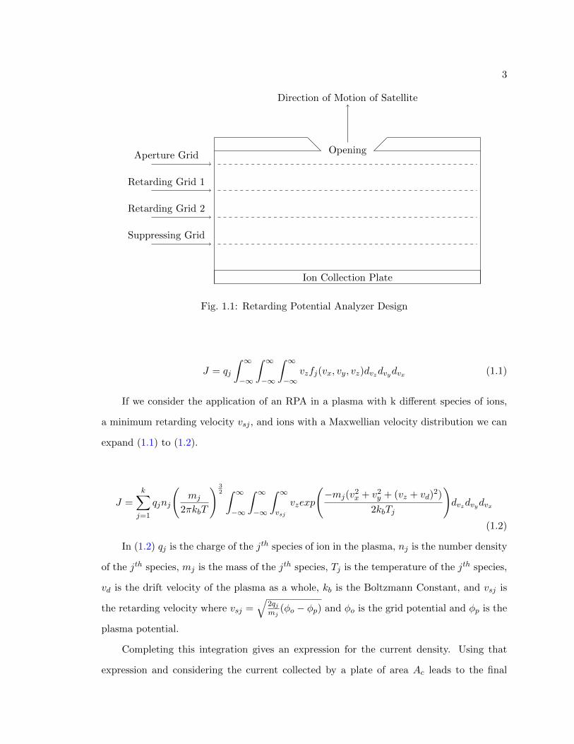
The key components of an RPA include wire-mesh grids to which a voltage is applied,

a current collector plate, and an opening in the direction of motion (ram direction) of the

satellite. A visualization of an RPA is shown in Fig. 1.1. The instrument is placed on a

spacecraft such that the opening is in line with the ram direction of the satellite. The grids

shown in Fig. 1.1 are not all necessary for an RPA to function, as some RPAs don’t use

an aperture grid and some only use one retarding grid. A negative voltage is applied to

the suppressing grid to repel all electrons. The positive voltage applied to the retarding

grids sweeps across a range of values, reducing the number of ions that make it to the ion

collection plate as it is increased. This is because as the voltage is increased fewer incident

ions have the energy required to penetrate the grid and many will instead be repelled [7].

This interaction creates a system where all ions below a minimum retarding velocity get

repelled from the instrument and don’t make it to the current measuring ion collection

plate.

A current-voltage plot (I-V curve) can be made using the current measured on the ion

collection plate for a set of voltages applied to the retarding grids. From the I-V curve much

can be learned about the ions in a plasma. For example, the magnitude of the derivative

of the I-V curve is related to the ion energy distribution [8]. Additionally, using careful

curve-fitting, the ion concentration, temperature, mass ratios, and relative speed of the ions

can be inferred from the I-V curves [7].

The equation describing an I-V curve as a function of physical plasma parameters can

be derived from the current density equation [9]. The current density, J , resulting from

a plasma where the jth particle has charge qj collected by a flat plate is give by equation

(1.1) where vx, vy and vz are the components of the velocity vector of the ion and f(...)

is a distribution function of those components of the velocity vector. The velocity vector

component vz is chosen to be defined as the velocity in the negative of the ram direction of

the satellite.

3

Aperture Grid

Ion Collection Plate

Retarding Grid 1

Retarding Grid 2

Suppressing Grid

Opening

Direction of Motion of Satellite

Fig. 1.1: Retarding Potential Analyzer Design

J = qj

∫ ∞−∞

∫ ∞−∞

∫ ∞−∞

vzfj(vx, vy, vz)dvzdvydvx (1.1)

If we consider the application of an RPA in a plasma with k different species of ions,

a minimum retarding velocity vsj , and ions with a Maxwellian velocity distribution we can

expand (1.1) to (1.2).

J =k∑

j=1

qjnj

(mj

2πkbT

) 32 ∫ ∞−∞

∫ ∞−∞

∫ ∞vsj

vzexp

(−mj(v

2x + v2y + (vz + vd)2)

2kbTj

)dvzdvydvx

(1.2)

In (1.2) qj is the charge of the jth species of ion in the plasma, nj is the number density

of the jth species, mj is the mass of the jth species, Tj is the temperature of the jth species,

vd is the drift velocity of the plasma as a whole, kb is the Boltzmann Constant, and vsj is

the retarding velocity where vsj =√

2qjmj

(φo − φp) and φo is the grid potential and φp is the

plasma potential.

Completing this integration gives an expression for the current density. Using that

expression and considering the current collected by a plate of area Ac leads to the final

4

equation; that the current, I, measured in an RPA due to a plasma is (1.3).

I =1

2vdAc

k∑j=1

qjnj

[1 + erf

(√mj

2kbTj(vsj + vd)

)+

1

vd

√2kbTjπmj

exp

(− mj

2kbTj(vsj + vd)2

)](1.3)

1.3 History of The Ion Drift Meter

The key components of an IDM consists of an opening placed in the ram direction of

the satellite, an aperture grid with a positive voltage applied to it, a suppressing grid with

a negative voltage applied to it, and an ion collector plate. However, the collector plate is

segmented in the IDM as seen in Fig. 1.2. The aperture grid is used to screen out low mass

ions, making the interpretation of IDM data easier.

The RPA is able to measure the ion drift velocity component in the look direction of

the instrument (ram direction of the satellite), but cannot measure the ion drift velocity

components in the other two orthogonal directions [6]. This is where the IDM can be of

use. The ratio of currents to different collector plate segments allows direct calculation of

the ion arrival angle [5].

The total current collected by a segment of the ion collection plate is given by (1.4),

where q is the charge of incoming ions, N is the ion density, A is the area of the plate,

χ is the transparency of the grid stack, and V is the velocity of the incoming particles

perpendicular to the plate.

I = qNAχV (1.4)

Understanding that the current to any segment of the collector plate is proportional

to the illuminated area leads to an expression for the ratio of two currents [9]. That ratio

is based on the physical parameters θ, W , and D as given in (1.5). θ is the arrival angle of

the plasma, W is the width of the instrument opening, and D is the effective depth of the

instrument. A visualization of these parameters is shown in Fig. 1.3. This equation solved

5

for θ is given in (1.6).

R =I1I2

=W2 +D tan(θ)W2 −D tan(θ)

(1.5)

θ = tan−1

(W (1 −R)

2D(1 +R)

)(1.6)

IDM Opening

A B

DC

Collector Segments

Fig. 1.2: Ion Drift Meter Collector Segments

1.4 Small Satellites

Historically, satellites that have included RPAs and IDMs in their instrumentation

packages have traditionally been large satellites with substantial budgets. Some such mis-

sions are the Dynamics Explorer, [10], Communications/Navigation Outage Forecasting

System [11], and Defense Meteorological Satellite Program (DMSP) satellites [12].

Smaller cube satellites (CubeSats) have recently become popular as an alternative to

6

I1 I2

θIncoming Ions

D

W

Fig. 1.3: Ion Drift Meter Parameters

big satellites for conducting meaningful science missions at a lower cost. Some missions,

such as the Dynamic Ionosphere CubeSat Experiment (DICE) mission and Radio Aurora

Explorer mission [13], have proven the worth of the CubeSat model. Another benefit of

using CubeSats is that constellations of CubeSats (two or more) can be sent into orbit for a

fraction of the cost of a constellation of large satellites. Constellations can provide a more

detailed view of plasma processes with fewer spatial or temporal gaps in the collected data.

For these reasons, equipping CubeSats with plasma measurement instruments has become

an important area of research.

1.5 Previous Work Done on GRIDS

Mechanical and electrical design work has been previously done to combine the IDM

and RPA instrument functionality into one lightweight, small, low-power unit ideal for

small satellites [14]. This new instrument is called the Gridded Retarding Ion Distribution

Sensor (GRIDS). Testing has shown that the design, while saving on power and space,

does not compromise much in terms of instrument accuracy relative to using two separate

instruments. A picture of the built sensor head is shown in Fig. 1.4.

7

Fig. 1.4: The GRIDS Sensor Head

The electronics of GRIDS have already been picked out and have been placed on a

circuit board. A picture of these electronics is shown in Fig. 1.5. The FPGA chosen for

GRIDS is the AGLN250V5-VQG100 produced by the Microsemi Corporation. A quad

channel DAC, Linear Technology’s LTC2604, is used to produce the grid voltages GRIDS

requires to operate correctly. To measure the small currents encountered in normal op-

erations, the Texas Instrument’s DDC114 chip was chosen. The DDC114 chip is a 20-bit

precision quad channel current measurement device that takes measurements using a charge

accumulation method.

1.6 Project Goals

The goal of this thesis is to develop and test a Field Programmable Gate Array (FPGA)

design that provides the necessary instrument functionality. This includes sending out data

that GRIDS produces through a standard protocol with a well-defined packet structure,

8

Fig. 1.5: GRIDS Electronics

controlling the grid voltage levels, and implementing current sensing.

The old debug code that was previously developed operates in a very limited capacity

as can be seen on the left side of Fig. 1.6. The purpose of the debug code was to test the

basic functionality of the instrument and only implemented the current measurement part

of the design along with limited communications through a debug port.

The extent that the new prototype code operates is shown on the right side of Fig. 1.6.

The prototype code also implements current measurement, but adds automatic ranging

functionality to it. The prototype code implements a well defined packet structure and

outputs those packets over a RS-422 communication bus. The prototype code additionally

provides controls for the grid voltages. These features provide full instrument functionality

and their design will be discussed in detail in the following chapters.

9

Instrument

Initialization

Current Measurments

Current MeasurmentLoop

Debug Port

Power On

Debug Code

Instrument

Initialization

Current Measurment Loop

Range Sensing loop

Packetizer

RS-422 Data Out

Current Measurments

Power On

Grid Voltage Control

DAC

Prototype Code

Voltage Levels

Fig. 1.6: Debug code functionality vs. Prototype code functionality

10

CHAPTER 2

FPGA DESIGN

2.1 Design Overview and Requirements

GRIDS takes measurements of plasma in two different ways, GRIDS enters RPA mode

to take the same measurements an RPA would, and IDM mode to take the same measure-

ments an IDM would. In the 50/50 mode of operation, GRIDS spends one half second in

RPA mode, then the subsequent half second in IDM mode, then repeats indefinitely. Much

of the operation of the instrument is the same during RPA mode and IDM mode, with

the exception of the grid voltages. RPA mode requires stepping grid voltages while IDM

mode does not. During both RPA and IDM modes, GRIDS takes current measurements,

determines if it needs to range, and reports the data to the packetizer system. The pack-

etizer system places the data into a well-defined packet structure and outputs that packet

to an RS-422 port. The output RS-422 bus would be connected to a spacecraft’s on-board

computer in normal operation. A list of requirements is given in the list below.

1. The grid voltages are set to the correct level during IDM mode.

• Aperture Grid: Non-zero constant

• Retarding Grid 1: Zero volts

• Retarding Grid 2: Zero volts

• Suppressing Grid: Negative twelve volts

2. The grid voltages are set to the correct level during RPA mode.

• Aperture Grid: Zero volts

• Retarding Grid 1: Ramping voltage

• Retarding Grid 2: Ramping voltage

11

• Suppressing Grid: Negative twelve volts

3. Ensure current measurements don’t overlap from one voltage step to the next during

RPA mode.

4. Ignore current measurements that take place during voltage rise time during RPA

mode.

5. Report 100 current measurements in the telemetry every second; 50 in RPA mode

and 50 in IDM mode.

6. Implement an automatic current range sensing system.

7. Define a packet structure for data output from the system.

8. Follow the defined packet structure when outputting data from the system.

9. Create code that communicates through the standard RS-422 protocol.

10. Ensure the full code can be implemented on the FPGA.

11. Implement a secondary mode for GRIDS based on taking 10 sets of measurements a

second.

2.2 FPGA Parameters

An FPGA was chosen as the computing chip for GRIDS because of the accurate timing

FPGAs are known for, the lack of complex math operations required to run the instru-

ment, and the available low-power FPGA options. The FPGA that GRIDS uses is the

AGLN250V5-VQG100 produced by the Microsemi Corporation. This FPGA is a part of

Microsemi’s IGLOO nano device line. The space available on the AGLN250V5-VQG100 is

6144 core cells, eight 4608-Bit RAM blocks, and 68 input/output ports. All of the FPGA

code for GRIDS needs to be designed such that it fits within these resource constraints.

12

2.3 Grid Voltage / DAC

GRIDS has four electrically isolated grids that each need to be driven separately. A

quad channel DAC, Linear Technology’s LTC2604, is used to produce these grid voltages.

These grids operate differently depending on the instrument mode (RPA or IDM). A concept

of operations for the instrument is shown in Fig. 2.1. This figure details how the four

different grid voltages operate during RPA and IDM modes, while additionally showing

that the instrument runs in RPA mode for half a second, then IDM mode for half a second,

then repeats.

During RPA mode: the aperture grid is set to zero volts, retarding grids 1 and 2 both

step 50 times at even intervals between 0 and 12 volts, and the suppressing grid is set to

-12 volts.

During IDM mode: the aperture grid is set to a non-zero constant voltage, retarding

grids 1 and 2 are set to zero volts, and the suppressing grid is set to -12 volts.

2.4 Current Sensing / DDC chip

GRIDS measures four currents, one for each segment of the segmented current collector.

These four current measurements are used separately to reconstruct IDM data and added

together into one measurement to reconstruct RPA data. Texas Instrument’s DDC114 chip

is a 20 bit precision quad channel current measurement device. The DDC114 chip measures

current by charging a capacitor for an amount of time, the integration time. The level of

charge on the capacitor along with the integration time are used to determine the average

current measured over that time. As a result of the DDC114 chip using charge accumulation

to measure currents, the charge accumulators saturate at lower current values with a long

integration timer than they would if the integration timer was short.

The DDC114 chip can only measure two currents at a time. The DDC CONV signal

(labeled Integration Channel) shown in Fig. 2.2 indicates both which two currents are being

measured and how long the integration timer is. In order to get a measurement of all four

currents the DDC CONV signal needs to be both high and low for the same time, so all

four currents are measured for the same integration time.

13

...T = 0 s T = 0.5 s T = 1 s T = 1.5s T = 2s

Data Packet

Generated

Data Packet

Generated

Data Packet

Generated

Data Packet

Generated

Time

Scale

RPA Mode IDM Mode

Retarding

Grid 1

RPA Mode IDM Mode

Ramping Voltage

Ramping Voltage

Constant -12 V

Zero Volts

Zero Volts

Constant -12 VSuppressing

Grid

Aperture

GridZero Volts Zero Volts

Non-Zero Constant Non-Zero Constant

Ramping Voltage

Zero Volts

Ramping Voltage

Zero Volts

Constant -12 V Constant -12 V

Retarding

Grid 2

Fig. 2.1: Voltage Grid DAC Function

14

After the DDC CONV signal changes, there is a delay of 1380 clocks (from the clock

running the DDC114 chip) before the two currents the DDC114 chip just measured are

placed in the output data registers. The DDC DValid signal then pulses indicating that the

digitized current values are ready to be read out of the data registers. The DDC114 chip’s

data register is 80-bits long and only updates the relevant 40-bits when the DDC Dvalid

signal pulses. Because of this, the instrument waits until after the DDC CONV signal has

gone high and low before reading out the data to ensure all four current measurements are

present in the data registers.

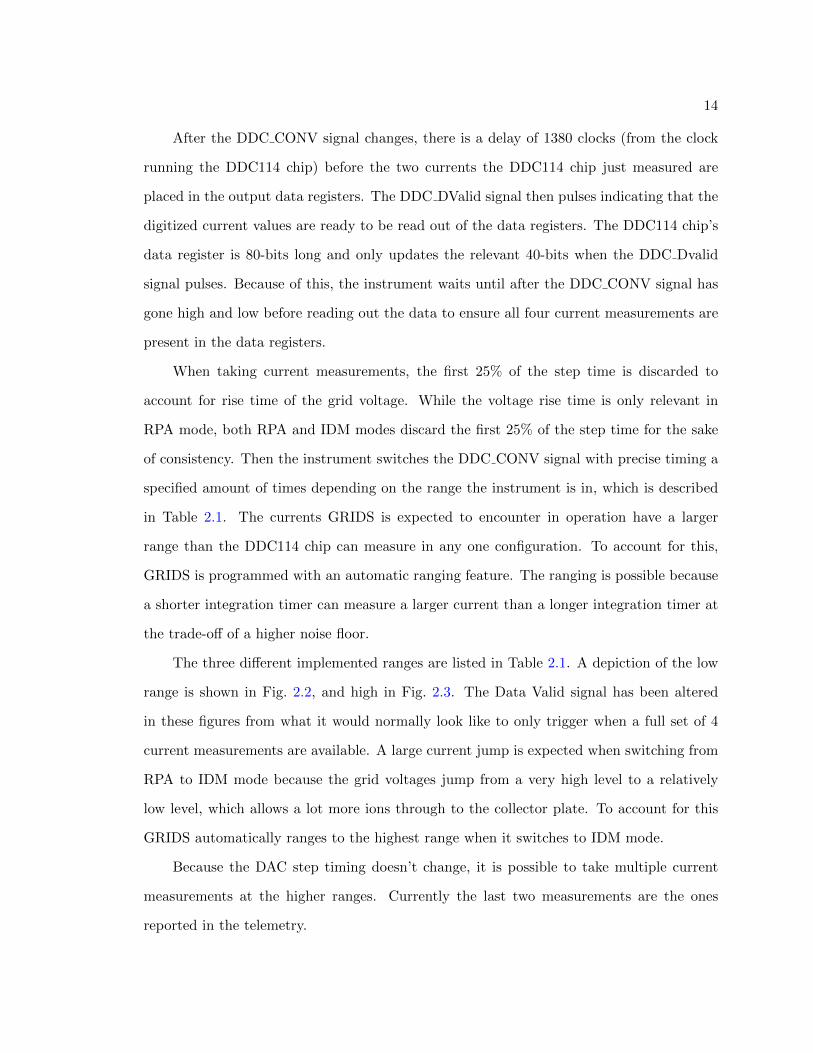
When taking current measurements, the first 25% of the step time is discarded to

account for rise time of the grid voltage. While the voltage rise time is only relevant in

RPA mode, both RPA and IDM modes discard the first 25% of the step time for the sake

of consistency. Then the instrument switches the DDC CONV signal with precise timing a

specified amount of times depending on the range the instrument is in, which is described

in Table 2.1. The currents GRIDS is expected to encounter in operation have a larger

range than the DDC114 chip can measure in any one configuration. To account for this,

GRIDS is programmed with an automatic ranging feature. The ranging is possible because

a shorter integration timer can measure a larger current than a longer integration timer at

the trade-off of a higher noise floor.

The three different implemented ranges are listed in Table 2.1. A depiction of the low

range is shown in Fig. 2.2, and high in Fig. 2.3. The Data Valid signal has been altered

in these figures from what it would normally look like to only trigger when a full set of 4

current measurements are available. A large current jump is expected when switching from

RPA to IDM mode because the grid voltages jump from a very high level to a relatively

low level, which allows a lot more ions through to the collector plate. To account for this

GRIDS automatically ranges to the highest range when it switches to IDM mode.

Because the DAC step timing doesn’t change, it is possible to take multiple current

measurements at the higher ranges. Currently the last two measurements are the ones

reported in the telemetry.

15

DAC rise time,

25% total step

time

75% of step,

measure

DDC_CONV

DAC

Data Valid

Discarded Reported

Data

A B A B

Fig. 2.2: Current measuring functionality at a slow measurement rate

DAC rise time,

25% total step

time

75% of step,

measure

DDC_CONV

DAC

Discarded Ignore Ignore Ignore

Data Valid

A B A B A B A B A B

Reported

Data

Fig. 2.3: Current measuring functionality at a fast measurement rate

16

Table 2.1: List of ranges for current sensing.

Range Current Measurable Time spent per DDC CONV signal # of DDC CONV toggles

Low 0-35nA 3.73 ms 2

Medium 20-90nA 1.87 ms 4

High 70-300nA 0.94 ms 8

2.5 Packetizer

The Packetizer code takes the data produced by GRIDS and orders it into packets.

Having well defined data packets is common practice for space instruments since many on-

board computers on spacecraft require it. The on-board computer is responsible for, among

other things, taking data output by all of the spacecraft’s various subsystems and organizing

it into a format ready for radio downlink. Packets of fixed length or packets that contain

information about their length in the header make this job much easier for the on-board

computer. These packets are then parsed on the ground to retrieve the data produced by

the subsystems.

The packet structure for GRIDS is defined in figure Fig. 2.4. Each packet always starts

with a header which begins with a sync word. The sync word is 4 bytes, and is meant to

help later packet parsing efforts. The next 4 bytes is the Packet Number Counter, which

is a simple counter that is incremented by 1 every time a packet is generated by GRIDS.

Next is the Packet Length, which holds information on how many bytes make up the whole

packet. The rest of the header is made up of eight 2-byte values that contain various

housekeeping information, such as voltage levels and temperature levels. The last of these

2-byte values labeled DDC RANGE contains information on the DDC114 current sensor

chip that is critical for converting the raw data into currents.

After the header is the data portion of the packet, which makes up the bulk of the

packet. The data portion is made up of many 20-byte chunks that contain pertinent in-

formation for a single current measurement. First, the value of all four grid voltage levels

is reported in a series of four 2-byte values. Then the next 10 bytes are used for the raw

DDC114 chip data values. Because the DDC114 chip has 20-bit resolution and we are

17

measuring four currents there is a total of 80 bits of data reported every time a current

measurement is taken. These four 20-bit measurements are placed one next to the other

in the 10 byte data chuck as shown in Fig. 2.5. The last item is a 2-byte value containing

the integration timer, represented as counts of a 10MHz clock. Because there are 50 data

values reported per packet this makes the length of a total packet 1026 bytes.

The original design for the packetizer was to store all the data for a packet in RAM

then to output all the data sequentially without delay. The FPGA hardware, however,

ended up not supporting this design. The RAM module included in the FPGA was unable

to store all the data required for a packet. This issue lead to the current design where the

data is output as it is available rather than all at once. Using careful timing, the structure

of the packet remains intact, despite the hardware limitations.

Fig. 2.4: Packet Structure

Fig. 2.5: Definition of data field from the packet structure

18

2.6 10 Hz mode

In addition to the primary mode of operation for GRIDS (the 50/50 mode) another

operational mode labeled the 10 Hz mode was designed. The 10 Hz mode takes 200 mea-

surements total in a second following a structure of 16 RPA measurements followed by 4

IDM measurements, with that being repeated 10 times in a second.

In 10 Hz mode the aperture and suppressing grids are still set to the same values as

in 50/50 mode. The retarding grids still step over the whole voltage range during RPA

mode, just using a larger step size since the instrument runs for the duration of 16 RPA

measurements instead of 50. The retarding grids are set to the same values during IDM

mode as they are in 50/50 mode.

The 10 Hz mode also requires changes to the packet structure. Both the 50/50 mode

and 10 Hz mode use the same packet header and the same structure for the data portion

of the packet but the number of measurements reported per packet changes. Instead of

generating a packet of data every half second like in 50/50 mode, the 10 Hz mode generates

a total of 20 packets in a second with 10 packets containing RPA data and the other 10

containing IDM data. While both IDM and RPA packets each contain 50 measurements

in 50/50 mode, in the 10 Hz mode IDM packets contain 4 sets of measurements and RPA

packets contain 16 sets of measurements. This makes 10 Hz mode IDM packets 106 bytes

long and RPA packets 346 bytes.

The rest of the instrument functions the same in both 50/50 mode and 10 Hz mode. The

same hardware is used, GRIDS still automatically ranges based on the measured current,

and the packets are still output on the RS-422 port. 10 Hz mode was designed to take faster

measurements than in 50/50 mode, hopefully with the ability to reveal new structures in

plasma due to the higher temporal resolution.

2.7 Toolchain

Typical FPGA programming involves writing code using the VHDL or Verilog lan-

guages. This project takes a different approach and uses Matlab Simulink code. Routing

the Simulink files through Matlabs HDL auto-coder converts Simulink code into an HDL file

19

that Libero, Microsemi’s FPGA design software, can utilize. Libero runs place and route

and compiles the code into a programming file. Place and route is a process integral to

FPGA design where first the electronic components, circuitry and logic elements are placed

on a FPGA fabric where there is limited space. Then routing decides the design of all

the wires needed to connect the components placed in the previous step. Finally a utility

program called FlashPro takes the programming data file (PDB) that Libero generated and

loads it onto the FPGA. This process is shown in figure Fig. 2.6.

Matlab Simulink

Code subsystem functionality

Matlab HDL Coder

Create HDL file from Simulink code

Libero

Connect SubsystemsManage Wire Tracing

Libero Compiler

Create .PDB file from project in Libero

FlashPro

Program FPGA based on .PDB file

FPGA ON BOARD

EXECUTES PROGRAM

Fig. 2.6: Coding Toolchain

Two major benefits are gained through coding an FPGA this way. The first is the

powerful simulation capabilities that Matlab Simulink provides. The ability to simulate

code before testing it on an FPGA is integral to writing high quality code quickly and

makes many bugs easier to find and fix. The second main benefit is that this toolchain is

much easier to learn and use for an individual untrained in FPGA design.

20

CHAPTER 3

FPGA Testing

3.1 Requirement Completeness and Test Setup

A list of the requirements from Chapter 2 is below along with an indication on their

current working level.

1. The grid voltages are set to the correct level during IDM mode.

• Aperture Grid: Non-zero constant Partially Working

• Retarding Grid 1: Zero volts Working

• Retarding Grid 2: Zero volts Working

• Suppressing Grid: Negative twelve volts Working

2. The grid voltages are set to the correct level during RPA mode.

• Aperture Grid: Zero volts Partially Working

• Retarding Grid 1: Ramping voltage Working

• Retarding Grid 2: Ramping voltage Working

• Suppressing Grid: Negative twelve volts Working

3. Ensure current measurements don’t overlap from one voltage step to the next during

RPA mode. Working

4. Ignore current measurements that take place during voltage rise time during RPA

mode. Working

5. Report 100 current measurements in the telemetry every second; 50 in RPA mode

and 50 in IDM mode. Working

21

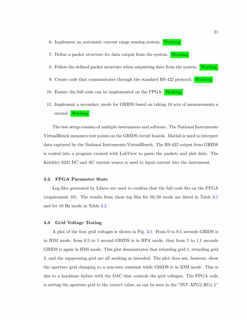
6. Implement an automatic current range sensing system. Working

7. Define a packet structure for data output from the system. Working

8. Follow the defined packet structure when outputting data from the system. Working

9. Create code that communicates through the standard RS-422 protocol. Working

10. Ensure the full code can be implemented on the FPGA. Working

11. Implement a secondary mode for GRIDS based on taking 10 sets of measurements a

second. Working

The test setup consists of multiple instruments and software. The National Instruments

VirtualBench measures test points on the GRIDS circuit boards. Matlab is used to interpret

data captured by the National Instruments VirtualBench. The RS-422 output from GRIDS

is routed into a program created with LabView to parse the packets and plot data. The

Keithley 6221 DC and AC current source is used to input current into the instrument.

3.2 FPGA Parameter State

Log files generated by Libero are used to confirm that the full code fits on the FPGA

(requirement 10). The results from these log files for 50/50 mode are listed in Table 3.1

and for 10 Hz mode in Table 3.2.

3.3 Grid Voltage Testing

A plot of the four grid voltages is shown in Fig. 3.1. From 0 to 0.5 seconds GRIDS is

in IDM mode, from 0.5 to 1 second GRIDS is in RPA mode, then from 1 to 1.1 seconds

GRIDS is again in IDM mode. This plot demonstrates that retarding grid 1, retarding grid

2, and the suppressing grid are all working as intended. The plot does not, however, show

the aperture grid changing to a non-zero constant while GRIDS is in IDM mode. This is

due to a hardware failure with the DAC that controls the grid voltages. The FPGA code

is setting the aperture grid to the correct value, as can be seen in the ”INT APG2 RG1 1”

22

Table 3.1: List of FPGA parameters for 50/50 mode.

Item Total Available Used Does it fit

Core Cells 6144 4540 Yes

I/O ports 68 26 Yes

RAM blocks 8 4 Yes

Table 3.2: List of FPGA parameters for 10 Hz mode.

Item Total Available Used Does it fit

Core Cells 6144 4313 Yes

I/O ports 68 26 Yes

RAM blocks 8 4 Yes

column in Fig. 2.5. This is why requirements 1 and 2 have the aperture grid labeled as

partially working, and the other grids labeled as working. Correcting the hardware failure

would result in the desired functionality without any code changes.

3.4 Current Sensing Testing

To test the current sensing portion of GRIDS the Keithley 6221 DC and AC current

source was used to input a sine wave with 0-120 nA amplitude and 4 Hz frequency into

GRIDS. A plot of one packet worth of DDC114 counts is shown in Fig. 3.2. The shape of a

sine wave can easily be made out in this picture, but there are also two jagged jumps per

curve. These jumps are due to the automatic ranging system changing the integration time.

The DDC114 chip’s 20-bit resolution means that the DDC114 counts can be any number

between 0 and 1,048,575. To convert the DDC114 counts to a current, equation (3.1) is

used. RawV alue is the 20-bit value generated by the DDC 114 chip, Offset is equal to

4096, Capacitance is 300pF, and IntegrationT ime changes based on what the automatic

ranging is set to, but can be equal to 3.73 ms, 1.87 ms, or 0.94 ms.

Current =(RawV alue−Offset) ∗ Capacitance

IntegrationT ime ∗ 220(3.1)

A plot of the DDC114 counts converted into a current is shown in Fig. 3.3. This

23

0 0.1 0.2 0.3 0.4 0.5 0.6 0.7 0.8 0.9 1 1.1−15

−10

−5

0

5

10

15

Time (s)

Vol

tage

(V)

Grid Voltage 50/50 Mode

Aperture GridRetarding Grid 1Retarding Grid 2Suppressing Grid

Fig. 3.1: Plot of the four grid voltages with GRIDS configured for 50/50 mode, data recordedfor 1.1 seconds

24

0 5 10 15 20 25 30 35 40 45 500

0.1

0.2

0.3

0.4

0.5

0.6

0.7

0.8

0.9

1

1.1·106

Time Index

DD

C11

4C

ount

Raw Measured Values

Fig. 3.2: Raw Values

25

meets requirement 6, implementing an automatic range sensing system, because the current

measured by GRIDS matches the input current and ranging is shown happening in Fig. 3.2.

0 5 10 15 20 25 30 35 40 45 500

0.2

0.4

0.6

0.8

1

1.2

1.4

·10−7

Time Index

Cu

rren

t(A

)

Measured Current

Fig. 3.3: Reconstructed Current

Another plot that demonstrates the automatic ranging functionality is presented in

Fig. 3.4. This plot contains the voltage steps from retarding grid 1 during RPA mode,

and the DDC CONV signal that is generated during that same time. In this figure the

DDC CONV signal can be seen to switch from medium range to low range later in the plot.

This figure also shows requirement 3, that the current measurements don’t overlap from

one voltage step to the next, is met. It can be seen that the DDC CONV signal doesn’t

drift in relation to the stepping voltage.

Requirement 4, that GRIDS ignores current measurements during the voltage rise time,

can also be shown to be complete by taking a closer look at Fig. 3.5. The DDC CONV

26

signal switches from high to low in the first 25% of the step time to account for the grid

voltage rise time, just like the intended function detailed in Fig. 2.2. It’s thus concluded

that current measurements made during the rise time aren’t reported.

0.00 0.01 0.02 0.03 0.04 0.05 0.06 0.07 0.08 0.09 0.100

0.1

0.2

0.3

0.4

0.5

0.6

0.7

0.8

0.9

Time (s)

Vol

tage

(V)

DDC CONV signal and Retarding Grid 1

0.00 0.01 0.02 0.03 0.04 0.05 0.06 0.07 0.08 0.09 0.10

Low

High

Con

vers

ion

Sig

nal

Retarding Grid 1DDC CONV

Fig. 3.4: Plot of Retarding Grid 1 overlaid with the DDC CONV with GRIDS configuredfor 50/50 mode, data recorded for 0.1 seconds

3.5 Packetizer Testing

Requirement 7, defining a packet structure, is complete and shown in Fig. 2.4 and Fig.

2.5.

To test that the packetizer functions correctly a LabView parser program was created.

The parser program reads in the data packets output by GRIDS, and parses the packet to

retrieve the embedded data. The packet structure was described to Dr. Ryan Davidson,

who used that information to create the parsing program in LabView. A picture of that

27

25% 75%

Fig. 3.5: Zoomed in plot of the same data from Fig. 3.4 with annotations added

28

LabView program with a packet containing IDM data is shown in Fig. 3.6. Completeness

of requirement 8, which requires GRIDS data output following a defined packet structure,

is demonstrated as a parsing program created to the specifications of the packet structure

was able to retrieve the data embedded in the packet. Requirement 5, which requires 100

current measurements reported every second, is also shown to be completed as the packet

structure defines 50 current measurements in RPA mode, and 50 current measurements in

IDM mode, which each take half a second to complete. The parsing program based on this

packet structure corroborates this.

Fig. 3.6: LabView program showing data parsed from a packet containing IDM data

The packet output of GRIDS was connected to a computer running the LabView pars-

ing program using an RS-422 to USB cable. The fact that the LabView program received the

data through this cable shows completeness of requirement 9, which requires that GRIDS

sends data packets using the RS-422 protocol.

3.6 10 Hz mode Testing

A plot of the grid voltages when GRIDS is in the 10 Hz mode is shown in Fig. 3.7.

Because the 10 Hz mode is run on the same hardware as 50/50 mode, the aperture grid

is not shown functioning properly for the same reasons the aperture grid doesn’t function

29

properly in 50/50 mode. A more detailed view of the function of the grid voltages during

10 Hz mode is shown in Fig. 3.8. In this figure GRIDS is in IDM mode from 0.0 to 0.02

seconds, then RPA mode from 0.02 to 0.1 second, then repeats with IDM mode from 0.1 to

0.12 seconds and RPA mode from 0.12 to 0.20 seconds. This timing is consistent with the

goal of requirement 11, producing 10 sets of measurements per second. However, there is a

hardware issue in regards to the response time of the grid voltages as the retarding grids

are supposed to be set to 0 volts for the duration of IDM mode. In Fig. 3.8 it is observable

that the time it takes for the voltage to fall from 12 volts to 0 volts at the transition of RPA

mode to IDM mode takes long enough to interfere with IDM mode measurements.

The packetizer system for 10 Hz mode was also tested with the LabView parsing pro-

gram, which shows it is working as intended. 0.2 seconds worth of data taken while GRIDS

was in 10 Hz mode is listed in appendix A.1. The rest of the function of the 10 Hz mode

matches that of the 50/50 mode and has already been shown to be functional.

30

0 0.1 0.2 0.3 0.4 0.5 0.6 0.7 0.8 0.9 1 1.1−15

−10

−5

0

5

10

15

Time (s)

Vol

tage

(V)

Grid Voltage 10 Hz Mode

Aperture GridRetarding Grid 1Retarding Grid 2Suppressing Grid

Fig. 3.7: Plot of the four grid voltages with GRIDS configured for 10 Hz mode, data recordedfor 1.1 seconds

31

IDM RPA RPAIDM

Fig. 3.8: Annotated plot of the four grid voltages with GRIDS configured for 10 Hz mode,data recorded for 0.2 seconds

32

CHAPTER 4

CONCLUSIONS AND FUTURE WORK

4.1 Conclusion

This thesis outlines the FPGA design and testing of the GRIDS instrument. GRIDS can

perform the same measurements as both the IDM and RPA in one small, low-weight, low-

power package suitable for CubeSats. The FPGA code was developed in Matlab Simulink,

ported to HDL using an auto-coder, then fed into Libero to run place and route. GRIDS

uses an FPGA to control a quad-channel DAC for setting grid voltages and to control a

quad-channel current sensing chip, the DDC114 chip. An automatic ranging system was

implemented in the current sensing part of the design. This was needed because the range of

currents GRIDS is expected to encounter in normal operation is larger than the capabilities

of the DDC114 chip to measure in any one configuration. A packet structure was created

and used to output the data GRIDS produces through a RS422 bus. Two modes of operation

were implemented, the 50/50 mode and 10 Hz mode. Through testing all of the desired

functionality listed in the requirements was shown to be met with the exception of the

aperture grid due to a hardware malfunction.

4.2 Future Work

The hardware that is shown in Fig. 1.5 is not the final version of the hardware. Some

parts such as the FPGA, housekeeping ADC, and signal filters are going to be updated.

The new FPGA should include phase-locked loops, to run the current sensing chip at it’s

fastest supported rate, and more RAM space to allow for implementation of packet buffering

before packet output. The housekeeping ADC should have enough channels to support all

housekeeping data signals without the need for a multiplexer. The new signal filters should

allow the voltage to fall faster when switching from RPA mode to IDM mode, and shorten

33

the voltage rise time to be within the first 25% of the step time. These hardware changes

will influence what future work needs to be done on the GRIDS FPGA code, along with

additional desired functionality. A list of known future work for the FPGA code of GRIDS

follows.

1. The FPGA code written for this thesis will need to be ported to a new FPGA other

than the currently used AGLN250V5-VQG100 from Microsemi Corporation. So long

as another FPGA made by Microsemi Corporation is used this hardware change should

only necessitate changing pin assignments in Libero.

2. Buffer a whole packets worth of data before outputting a packet. Packet data will be

able to be buffered once additional RAM space is available. The current implemen-

tation doesn’t store packet data in RAM and just outputs the data as it is created.

Correct implementation of packet output means that packet data will be stored in

RAM until a full packets worth of data is available for output.

3. FPGA code to implement the housekeeping data needs to be written. The housekeep-

ing data, which makes up much of the packet header, isn’t working currently. The

decision was made to not spend time implementing the housekeeping code because

much of the hardware surrounding the housekeeping data had plans to change.

4. Implement commanding to give additional control over GRIDS while on orbit. GRIDS

would receive commands through its RS-422 port, parse it, and execute the command.

Some examples of desired commands include the ability to change the value of the non-

zero constant that the aperture grid is set to during IDM mode, and to enable/disable

automatic ranging.

5. Add additional ranges for the ranging system to increase instrument accuracy. With

the addition of phase-locked loops in a new FPGA it should be possible to add ad-

ditional ranges for the ranging system. Also, supposing that the new hardware can

handle the calculations, averaging the multiple current measurements the DDC114

34

chip takes while in the high ranges during a single voltage step would be a desirable

function.

35

REFERENCES

[1] J. L. Barth, C. Dyer, and E. Stassinopoulos, “Space, atmospheric, and terrestrialradiation environments,” IEEE Transactions on Nuclear Science, vol. 50, no. 3, pp.466–482, 2003.

[2] V. Pisacane, The Space Environment and Its Effects on Space Systems, ser. AIAAeducation series. American Institute of Aeronautics and Astronautics, 2008. [Online].Available: https://books.google.com/books?id=se-QKAAACAAJ

[3] R. S. Conker, M. B. El-Arini, C. J. Hegarty, and T. Hsiao, “Modeling the effectsof ionospheric scintillation on gps/satellite-based augmentation system availability,”Radio Science, vol. 38, no. 1, 2003.

[4] C. Chao, S.-Y. Su, and H. Yeh, “Grid effects on the derived ion temperature and ramvelocity from the simulated results of the retarding potential analyzer data,” Advancesin Space Research, vol. 32, no. 11, pp. 2361–2366, 2003.

[5] R. Stoneback, R. Davidson, and R. Heelis, “Ion drift meter calibration and photoe-mission correction for the c/nofs satellite,” Journal of Geophysical Research: SpacePhysics, vol. 117, no. A8, 2012.

[6] M. Kelly. (2000) Ionospheric measurement techniques. [Online]. Available: https://cedarweb.vsp.ucar.edu/wiki/images/9/9e/Kelley 09.pdf

[7] L. Fanelli and e. al., “A versatile retarding potential analyzer for nano-satellite plat-forms,” Review of Scientific Instruments, vol. 86, no. 12, p. 124501, 2015.

[8] K. M. Lemmer, A. D. Gallimore, T. B. Smith, and D. R. Austin, “Review of tworetarding potential analyzers for use in high density helicon plasma,” in Proceedings ofthe 30th International Electric Propulsion Conference, Florence, Italy, 2007.

[9] R. Heelis and W. Hanson, “Measurements of thermal ion drift velocity and temperatureusing planar sensors,” Measurement techniques in space plasmas: particles, pp. 61–71,1998.

[10] W. Hanson, R. Heelis, R. Power, C. Lippincott, D. Zuccaro, B. Holt, L. Harmon, andS. Sanatani, “The retarding potential analyzer for dynamics explorer-b,” Space ScienceInstrumentation, vol. 5, pp. 503–510, 1981.

[11] J. D. Huba, R. W. Schunk, and Khazanov, Modeling the Ionosphere-Thermosphere.John Wiley & Sons, 2014, vol. 201.

[12] H. Fang and C. Cheng, “Retarding potential analyzer (rpa) for sounding rocket,” AnIntroduction to Space Instrumentation, edited by KI Oyama and CZ Cheng, pp. 139–153, 2013.

36

[13] H. Bahcivan, J. Cutler, M. Bennett, B. Kempke, J. Springmann, J. Buonocore,M. Nicolls, and R. Doe, “First measurements of radar coherent scatter by the radioaurora explorer cubesat,” Geophysical Research Letters, vol. 39, no. 14, 2012.

[14] W. S. Hatch, “Plasma velocity vector instruments for small satellites,” Master’s thesis,Utah State University, Logan, UT, 2016.

37

APPENDICES

38

Appendix A

Additional Data

A.1 10 Hz Packet Parser text output

INT APG2 RG1 1 INT RG2 1 INT RG3 1 INT SG 1 Integration Timer DDC 1 DDC

2 DDC 3 DDC 4 I1 (A) I2 (A) I3 (A) I4 (A)

0 0 0 65500 18668 0 4415 5182 4557 -6.277453E-10 4.888935E-11 1.664383E-10 7.065200E-

11

0 4090 4090 65500 18668 0 4413 0 2706 -6.277453E-10 4.858283E-11 -6.277453E-10

-2.130288E-10

0 8180 8180 65500 18668 0 4428 3365 4069 -6.277453E-10 5.088170E-11 -1.120317E-10

-4.137970E-12

0 12270 12270 65500 18668 0 4429 6560 5031 -6.277453E-10 5.103496E-11 3.776281E-10

1.432964E-10

0 16360 16360 65500 18668 0 4428 204 3119 -6.277453E-10 5.088170E-11 -5.964807E-10

-1.497332E-10

0 20450 20450 65500 18668 0 4410 953 3323 -6.277453E-10 4.812306E-11 -4.816903E-10

-1.184685E-10

0 24540 24540 65500 18668 0 4427 7472 5330 -6.277453E-10 5.072844E-11 5.173995E-10

1.891205E-10

0 28630 28630 65500 18668 0 4410 3097 3908 -6.277453E-10 4.812306E-11 -1.531049E-10

-2.881253E-11

0 32720 32720 65500 18668 0 4422 0 2847 -6.277453E-10 4.996215E-11 -6.277453E-10

-1.914194E-10

0 36810 36810 65500 18668 0 4418 5445 4707 -6.277453E-10 4.934912E-11 2.067452E-10

9.364072E-11

39

0 40900 40900 65500 18668 0 4420 4614 4445 -6.277453E-10 4.965564E-11 7.938772E-11

5.348709E-11

0 44990 44990 65500 18668 0 4411 0 2464 -6.277453E-10 4.827631E-11 -6.277453E-10

-2.501173E-10

0 49080 49080 65500 18668 0 4424 3855 4168 -6.277453E-10 5.026867E-11 -3.693521E-11

1.103459E-11

0 53170 53170 65500 18668 0 4409 7114 5120 -6.277453E-10 4.796980E-11 4.625331E-10

1.569363E-10

0 57260 57260 65500 18668 0 4431 55 3069 -6.277453E-10 5.134148E-11 -6.193161E-10

-1.573961E-10

0 61350 61350 65500 18668 0 4419 1961 3554 -6.277453E-10 4.950238E-11 -3.272061E-10

-8.306591E-11

35000 0 0 65500 9332 0 4411 4729 4499 -1.255760E-9 9.657332E-11 1.940664E-10

1.235525E-10

35000 0 0 65500 18668 0 4411 2803 3807 -6.277453E-10 4.827631E-11 -1.981628E-10

-4.429160E-11

35000 0 0 65500 18668 0 4426 0 2888 -6.277453E-10 5.057519E-11 -6.277453E-10 -

1.851358E-10

35000 0 0 65500 18668 0 4419 6167 4850 -6.277453E-10 4.950238E-11 3.173976E-10

1.155566E-10 0 0 0 65500 18668 0 4431 4749 4487 -6.277453E-10 5.134148E-11 1.000776E-

10 5.992393E-11

0 4090 4090 65500 18668 0 4403 0 2478 -6.277453E-10 4.705025E-11 -6.277453E-10

-2.479717E-10

0 8180 8180 65500 18668 0 4434 3394 4052 -6.277453E-10 5.180125E-11 -1.075872E-10

-6.743358E-12

0 12270 12270 65500 18668 0 4417 6445 4973 -6.277453E-10 4.919586E-11 3.600034E-10

1.344074E-10

40

0 16360 16360 65500 18668 0 4432 0 2979 -6.277453E-10 5.149473E-11 -6.277453E-10

-1.711893E-10

0 20450 20450 65500 18668 0 4407 1943 3570 -6.277453E-10 4.766328E-11 -3.299648E-10

-8.061378E-11

0 24540 24540 65500 18668 0 4441 7768 5389 -6.277453E-10 5.287406E-11 5.627639E-10

1.981628E-10

0 28630 28630 65500 18668 0 4411 2566 3776 -6.277453E-10 4.827631E-11 -2.344850E-10

-4.904260E-11

0 32720 32720 65500 18668 0 4431 0 2960 -6.277453E-10 5.134148E-11 -6.277453E-10

-1.741012E-10

0 36810 36810 65500 18668 0 4428 6100 4849 -6.277453E-10 5.088170E-11 3.071293E-10

1.154034E-10

0 40900 40900 65500 18668 0 4436 5080 4545 -6.277453E-10 5.210777E-11 1.508060E-10

6.881290E-11

0 44990 44990 65500 18668 0 4410 0 2801 -6.277453E-10 4.812306E-11 -6.277453E-10

-1.984693E-10

0 49080 49080 65500 18668 0 4419 3933 4196 -6.277453E-10 4.950238E-11 -2.498108E-11

1.532581E-11

0 53170 53170 65500 18668 0 4430 6897 5077 -6.277453E-10 5.118822E-11 4.292760E-10

1.503462E-10

0 57260 57260 65500 18668 0 4432 328 3108 -6.277453E-10 5.149473E-11 -5.774767E-10

-1.514190E-10

0 61350 61350 65500 18668 0 4416 1078 3363 -6.277453E-10 4.904260E-11 -4.625331E-10

-1.123382E-10

35000 0 0 65500 9332 0 4428 5618 4699 -1.255760E-9 1.017852E-10 4.666178E-10

1.848689E-10

35000 0 0 65500 18668 0 4418 2571 3801 -6.277453E-10 4.934912E-11 -2.337187E-10

-4.521115E-11

41

35000 0 0 65500 18668 0 4411 0 2788 -6.277453E-10 4.827631E-11 -6.277453E-10 -

2.004616E-10

35000 0 0 65500 18668 0 4417 5484 4721 -6.277453E-10 4.919586E-11 2.127223E-10

9.578634E-11