the fate of pops in the north sea -...
TRANSCRIPT

The Fate of Persistent Organic Pollutants in the North Sea
Multiple Year Model Simulations
of γ-HCH, α-HCH and PCB 153
Dissertation zur Erlangung des Doktorgrades
der Naturwissenschaften im Department für Geowissenschaften
der Universität Hamburg
vorgelegt von
Tatjana Ilyina
aus
Sankt Petersburg, Russland
Hamburg
2006

2
Als Dissertation angenommen von Department für Geowissenschaften der Universität Hamburg
Auf Grund der Gutachten von Prof. Dr. Jürgen Sündermann
und PD Dr. Gerhard Lammel
Hamburg, den 5 April 2006
Prof. Dr. Kay-Christian Emeis
Leiter des Departments für Geowissenschaften
Contents
3
Contents
CONTENTS ............................................................................................................... 3 ABSTRACT...................................................................................................................................... 7 ZUSAMMENFASSUNG................................................................................................................... 9
CHAPTER 1 ............................................................................................................... 11 INTRODUCTION AND BACKGROUND ..................................................................................... 11
1.1 Persistent organic pollutants (POPs): occurrence and effects ............................... 12 1.2 Legal instruments and measures to control POPs.................................................... 13 1.3 Approaches in POPs modelling .................................................................................. 16 1.4 POPs fate in the aquatic environment ....................................................................... 18 1.5 Objectives and outline of this study ........................................................................... 20
CHAPTER 2...............................................................................................................23 THE FATE AND TRANSPORT OCEAN MODEL (FANTOM): MODEL DESCRIPTION....... 23
2.1 Transport with ocean currents .................................................................................... 24 2.2 Air-sea exchange............................................................................................................ 25
2.2.1 Gaseous air-sea exchange...................................................................................... 26 2.2.2 Dry particle deposition.......................................................................................... 28 2.2.3 Wet deposition ....................................................................................................... 29
2.3 Phase distribution.......................................................................................................... 30 2.3.1 Particulate organic carbon content ...................................................................... 31 2.3.2 Fraction bound to particulate organic carbon.................................................... 33
2.4 Degradation in sea water .............................................................................................. 35
CHAPTER 3...............................................................................................................37 FANTOM: MODEL SETUP....................................................................................................... 37
3.1 Model area ...................................................................................................................... 38

Contents
4
3.2 Ocean circulation .......................................................................................................... 39 3.3 Compound selection..................................................................................................... 40
3.3.1 Gamma–hexachlorocyclohexane (γ–HCH) ....................................................... 42 3.3.2 Alpha–hexachlorocyclohexane (α–HCH) .......................................................... 43 3.3.3 Polychlorinated biphenyl 153 (PCB 153)............................................................ 44
3.4 Initial and boundary conditions .................................................................................. 45 3.4.1 Initialisation ............................................................................................................ 46 3.4.2 Oceanic boundary conditions .............................................................................. 46 3.4.3 River loads .............................................................................................................. 47 3.4.4 Atmospheric boundary conditions ...................................................................... 47 3.4.5 Data compilation and quality ............................................................................... 47
CHAPTER 4 ...............................................................................................................51 FANTOM: MODEL EVALUATION .......................................................................................... 51
4.1 Data used for model evaluation .................................................................................. 51 4.2 Comparison between modelled and measured sea water concentrations of γ-HCH..................................................................................................................................... 53 4.3 Comparison between modelled and measured sea water concentrations of α-HCH..................................................................................................................................... 58 4.4 Comparison between modelled and measured sea water concentrations of PCB 153 ................................................................................................................................. 62 4.5 Uncertainty and sensitivity analysis............................................................................. 67
CHAPTER 5 ...............................................................................................................71 OCCURRENCE AND PATHWAYS OF SELECTED POPS IN THE NORTH SEA....................... 71
5.1 Uptake of γ-HCH, α-HCH and PCB 153 by particulate matter in sea water....... 72 5.1.1 Distribution of particulate organic carbon in the North Sea........................... 72 5.1.2 Fraction of γ-HCH, α-HCH and PCB 153 on particulate organic carbon in sea water ......................................................................................................................... 75 5.1.3 γ-HCH, α-HCH and PCB 153 content in the liver of the North Sea flatfish dab (Limanda Limanda)....................................................................................... 79
5.2 Spatial and temporal distribution of γ-HCH, α-HCH and PCB 153 in sea water ............................................................................................................................ 81
5.2.1 γ-HCH horizontal and vertical distributions...................................................... 81 5.2.2 α-HCH horizontal and vertical distributions..................................................... 83 5.2.3 PCB 153 horizontal and vertical distributions ................................................... 85
5.3 α-HCH to γ-HCH ratio in sea water.......................................................................... 90

Contents
5
CHAPTER 6...............................................................................................................93 CONTRIBUTION OF INDIVIDUAL PROCESSES TO THE CYCLING OF SELECTED POPS IN THE NORTH SEA ................................................................................................................... 93
6.1 Mass budgets of γ-HCH, α-HCH and PCB 153 in the North Sea ........................ 94 6.1.1 Mass budget analysis for γ-HCH ......................................................................... 99 6.1.2 Mass budget analysis for α-HCH ......................................................................100 6.1.3 Mass budget analysis for PCB 153.....................................................................101
6.2 Residence time of γ-HCH, α-HCH and PCB 153 in sea water ............................103 6.3 Relative importance of some key processes for the fate of γ-HCH, α-HCH and PCB 153 in sea water ...................................................................................................105
6.3.1 The role of air-sea exchange, degradation, river and oceanic inflow............105 6.3.2 “Everything but one process” scenario analysis for γ-HCH..........................106 6.3.3 “Everything but one process” scenario analysis for α-HCH.........................107 6.3.4 “Everything but one process” scenario analysis for PCB 153.......................109 6.3.5 The role of temperature and wind speed in the air-sea gaseous exchange ..111
CHAPTER 7............................................................................................................. 115 CONCLUSIONS AND OUTLOOK .............................................................................................115
7.1 Conclusions..................................................................................................................115 7.2 Outlook.........................................................................................................................119
APPENDIX A........................................................................................................... 121
APPENDIX B........................................................................................................... 122
LIST OF FIGURES.................................................................................................. 123
BIBLIOGRAPHY .................................................................................................... 129
ACKNOWLEDGEMENTS ..................................................................................... 140

Contents
6

Abstract
7
Abstract
Persistent organic pollutants (POPs) are harmful to human health and to the environment. Their fate in the marine environment is not yet fully understood. The objective of this study is to advance the understanding about the fate of selected POPs in the marine environment as basis for higher accuracy estimates of their levels in the North Sea. An ocean model (FANTOM) has been developed to investigate the fate of selected POPs in the North Sea. The main focus of the model is on quantifying the distribution of POPs and their aquatic pathways within the North Sea. Key processes are three-dimensional transport of POPs with ocean currents, diffusive air-sea exchange, wet and dry atmospheric depositions, phase partitioning, degradation, and net sedimentation in bottom sediments. This is the first time that a spatially resolved, measurement-based ocean transport model has been used to study POP-like substances, at least on the regional scale.
The model was applied for the southern North Sea and tested by studying the behaviour of γ-HCH, α-HCH and PCB 153 in sea water in the years 1995 to 2001. The model’s structure and processes are described in details. Concentrations of γ-HCH, α-HCH and PCB 153 and their fluxes between upper sediment, sea and atmosphere were modelled, based on discharge and emission estimates available through various monitoring programmes.
Model results are evaluated against measurements. Modelled concentrations of the three selected POPs in sea water are in good agreement with the observations. The spatial distribution and the downward trend of the two HCHs in the entire North Sea are reproduced during the simulation period. The pathways of γ-, α-HCH and PCB 153 in the North Sea, were investigated suggesting the importance of the temperature dependence of the air-sea exchange. Model results showed that for the North Sea as a whole the air-sea flux is depositional, whereas in the German Bight it can be net volatilisational. For PCB 153, for the German Bight and for the whole North Sea net volatilisational flux also occurred. Model experiments suggest that the flux direction and magnitude is altered significantly by the Henry’s law coefficient temperature dependency, which could be responsible for more than 50% of the variability in the sea

Abstract
8
water concentrations of the studied POPs. Uptake by particulate matter in sea water was the most important for PCB 153 with up to 90% of the total concentration being on particles, whereas for the two HCHs this fraction was below 2% during entire simulation period.
For the first time mass budgets of γ-, α-HCH and PCB 153 in the North Sea and in the German Bight were calculated based on a modelling study. Calculated mass budgets show that γ-HCH and PCB 153 are controlled predominantly by the local sources, whereas for α-HCH transport form remote sources is probably the major source for the North Sea environment. This model study proves that transport models, such as FANTOM are capable to reproduce realistic multi-year temporal and spatial trends of selected POPs and can be used to address further scientific questions.

Zusammenfassung
9
Zusammenfassung
Persistente organische Schadstoffe (POPs) gefährden Mensch und Umwelt. Dennoch ist ihr Verhalten in der marinen Umgebung nur unzureichend verstanden. Ziel der vorliegenden Arbeit ist es daher, anhand eines weiterentwickelten numerischen Ozeanmodells (FANTOM) die Transportvorgänge von POPs im Meer besser zu verstehen und die Belastung der Nordsee abschätzen zu können. Das Modell berechnet die zeitliche und räumliche Ausbreitung von POPs innerhalb des Wasserkörpers der Nordsee. Die Schlüsselprozesse des Modells sind der dreidimensionale Transport durch Meeresströmungen, diffusiver Austausch zwischen Luft und Wasser, nasse und trockene atmosphärische Deposition, Aufnahme von POPs durch Schwebstoffe, sowie Sedimentation und Abbau. Im regionalen Bereich ist dieses räumlich auflösende, auf Messwerten basierende, ozeanographische Transportmodell zur Untersuchung von POPs das erste seiner Art.
Das Modell wurde für die südliche Nordsee angewandt und mit Simulationen von Ausbreitungsvorgängen von γ-HCH, α-HCH und PCB 153 für die Jahre 1995-2001 getestet. Die Struktur des Modells und dessen zu Grunde liegende Prozesse wurden detailliert beschrieben. Konzentrationen von γ-HCH, α-HCH und PCB 153 innerhalb des Wasserkörpers und deren Austausch an den Grenzflächen Luft, Boden und zu den benachbarten Gewässern wurden auf Grundlage von verfügbaren Eintragsschätzungen aus Monitoring-Programmen modelliert.
Die Evaluierung des Modells erfolgte durch einen Vergleich der simulierten täglichen Konzentrationen von HCHs und PCB 153 mit Messdaten und weist eine gute Übereinstimmung auf. Die räumliche Verbreitung sowie die generelle Abnahme der HCH-Belastung in der gesamten Nordsee im Laufe der Simulationsperiode zeigen sowohl Simulations- als auch Messdaten. Die Untersuchung der Transportwege von γ-, α-HCH und PCB 153 in der Nordsee erlauben eine Einzelbetrachtung der beeinflussenden Prozesse. So wurde die große Bedeutung der Temperaturabhängigkeit des Austausches zwischen Luft und Wasser festgestellt. Die Modellergebnisse zeigen weiterhin, dass die südliche Nordsee HCH über den Luft-Wasser-Austausch aufnimmt, die Deutsche Bucht jedoch über Volatilisierung HCH abgibt. Im Falle von PCB 153

Zusammenfassung
10
kann sogar in der gesamten Nordsee die Volatilisierung überwiegen. Die Modellergebnisse weisen darauf hin, dass sowohl die Flussrichtung zwischen Luft und Wasser als auch deren Größenordnung durch die Temperaturabhängigkeit des Henry-Koeffizienten bestimmt werden. Der Henry-Koeffizient könnte für 50% der Variabilität der Wasserkonzentrationen von POPs verantwortlich sein. Die Aufnahme von POPs durch absinkende Schwebstoffe ist bei PCB 153 besonders ausgeprägt, weil der Anteil der Gesamtkonzentration an Schwebstoffteilchen 90% ist. Für beide HCH-Isomere ist dieser Anteil während der gesamten Simulationsperiode unter 2%.
Erstmalig wurden basierend auf einer Modellstudie Massenbilanzen von γ-HCH, α-HCH and PCB 153 für die Nordsee und die Deutsche Bucht berechnet. Die Ergebnisse weisen darauf hin, dass γ-HCH und PCB 153 überwiegend von lokalen Einträgen bestimmt werden, während für α-HCH Ferntransport sehr wichtig ist. Die hier beschriebene Modellstudie beweist, dass Transportsmodelle wie FANTOM imstande sind, die räumliche und zeitliche Verbreitung von ausgewählten POPs in einer realistischen Weise zu reproduzieren und eine Vielzahl von Anwendungen finden können, um weitere wissenschaftliche Fragestellungen zu erörtern.

Chapter 1 Introduction and Background
11
Chapter 1
Introduction and Background
Awareness about persistent organic pollutants (POPs) began in the 1960-s with the publication of Rachel Carson's book “Silent Spring” where evidence of harmful effects of DDT (dichlorodiphenyltrichloroethane) on marine mammals and birds were documented.
The fate and behaviour of POPs in the environment has attracted considerable scientific and political interest arising from concern over human exposure to these chemicals and their discovery in pristine environments far from their source regions (Section 1.1). The ability of certain POPs to undergo long-range transport (LRT) has resulted in international actions to reduce and eliminate releases of these chemicals and to reduce the risks to regional and global environments (Section 1.2). International protocols require criteria for assessing the environmental risk posed by POPs based on sound scientific knowledge and models (Section 1.3).
The knowledge of processes and pathways that POPs undergo in the aquatic environment is of specific importance as it is the hydrosphere where POPs in many cases resist degradation and are more prone to bioaccumulation and, thus are more hazardous to living organisms (AMAP, 1998). However, the present knowledge of the processes which control the distribution and fate of POPs in the aquatic environment in general and in the North Sea in particular is clearly insufficient (Section 1.4).
These issues motivated the present study which aimed at advancing the knowledge on the fate of POPs in shelf seas by modelling their environmental behaviour and identifying the driving mechanisms of their cycling in sea water (Section 1.5).

Chapter 1 Introduction and Background
12
1.1 Persistent organic pollutants (POPs): occurrence and effects Persistent organic pollutants (POPs) are synthetic organic chemical compounds which are environmentally persistent, bioaccumulative and toxic. They are released into the environment through a range of processes including release during the industrial production, release during use (e.g. pesticides in agriculture), or release during combustion (e.g. dioxins). POPs have a particular combination of physical and chemical properties that ensure that once they have been released into the environment, they remain intact for exceptionally long periods. Although POPs are mostly produced by anthropogenic processes, natural sources can be also significant for some compounds. For example, emission of polycyclic aromatic hydrocarbons (PAHs) into the atmosphere can occur from forests fires and volcanic eruptions.
POPs migrate between the different environmental compartments and are able to undergo long-range transport (LRT) by natural processes in both the atmosphere and in the ocean, thus becoming ubiquitous global contaminants. High levels of some POPs were detected in the Arctic far from regions where they were released (AMAP, 1998).
Historically, the chemicals that have provoked the greatest concern due to their hazardous effects on the marine environment are the chlorinated hydrocarbons. They include such well known substances as the pesticide DDT and the PCBs (widely used in electrical devices). Hexachlorocyclohexane (HCH) used in agriculture is the most abundant organochlorine pollutant in both the atmosphere and ocean waters.
Although there are many hundreds of different chemicals under the heading of chlorinated hydrocarbons (PCBs alone may consist of up to 209 distinct chemicals) many of them share a number of important properties. In particular, they are generally fairly toxic, they are persistent in the environment and they are bioaccumulative. Bioaccumulation (increase in concentration of a pollutant from the environment to the first organism in a food chain) refers to how pollutants enter a food chain; biomagnification (increase in concentration of a pollutant from one link in a food chain to another) refers to the tendency of pollutants to concentrate as they move from one trophic level to the next. Together these phenomena mean that even small concentrations of chemicals in the environment can find their way into organisms in high enough dosages to pose danger. In order for biomagnification to occur, the pollutant must be long-lived, mobile, soluble in fats and biologically active. If a pollutant is short-lived, it will be broken down before it can become dangerous. If it is not mobile, it will stay in one place and is unlikely to be taken up by organisms. If the pollutant is soluble in water it will be excreted by the organism.

Chapter 1 Introduction and Background
13
The greatest part of wildlife exposure to POPs is attributed to the food chain (AMAP, 1998). Contamination of food may occur through environmental pollution of air, water and soil, or through the previous use or unauthorized use of organochlorine pesticides on food crops. Episodes of massive food contamination have been reported. Some chlorinated hydrocarbon insecticides have been known to be the cause of serious, acute poisonings. Humans can be exposed to POPs through diet, occupation, accidents and the environment, including the indoor environment. It is believed that exposure to certain POPs can have the potential for a significant impact on human health either in the short or long term (WHO, 2003). High (over) exposures at the point of use of some POPs can lead to acute effects, including death, while at lower exposure levels long term effects can occur. In general, exposure to POPs, either acute or chronic, can be associated with a wide range of adverse health effects, including cancer, damage to the central and peripheral nervous systems, diseases of the immune system, reproductive disorders, and interference with infant and child development. However effects resulting from low level chronic exposure are yet to be understood. Human health impacts may be felt most acutely in populations that consume large amounts of fish (e.g., subsistence fishermen), since fish have a high fat content and thus can contain high concentrations of POPs.
Shifting from POPs to chemical and non-chemical alternatives is the key issue in reducing their impact. A high priority is finding alternatives to hazardous chemicals for insect control. POPs can be produced cheaply compared to most other industrial chemicals. There are many safer chemical and non-chemical alternatives, but their development and dissemination will require time, money, and training. For example, replacing DDT (widely used to control malarial mosquitoes) with less hazardous forms of insect control requires time to plan effective actions (e.g., integrated pest management systems, consisting of the sparing use of pest-specific pesticides and biological control methods).
1.2 Legal instruments and measures to control POPs
Although the first publication where toxic effects of POPs were addressed appeared in 1970 (Prest et al., 1970), it was only in 1995 when an international working group was convened by the UNEP1 Governing Council to develop assessments for 12 POPs, thus recognising the threat posed by this chemicals as a global problem which has to be dealt at an international level.
1United Nations Environment Programme: http://www.chem.unep.ch/pops/ (last visited 25 January 2006).
Chapter 1 Introduction and Background
14
Political interest in the fate and behaviour of POPs in the environment arises from concern over human exposure to these chemicals and to their discovery in pristine environments far from source regions (UNEP, 2003). The UNEP Stockholm Convention2, a global treaty to protect human health and the environment from POPs was open for signature/ratification in May, 2001. It forms a framework, based on the precautionary principle, which seeks to guarantee the safe elimination of these substances as well as reductions in their production and use. The Convention covers twelve priority POPs, although the eventual long-term objective is to cover other substances. These 12 POPs are aldrin, chlordane, dichlorodiphenyltrichlorethane (DDT), dieldrin, endrin, heptachlor, mirex, toxaphene, polychlorobiphenyls (PCBs), hexachlorobenzene, dioxins and furanes. The Convention entered into force in May 2005 and most of the twelve POPs currently addressed in international negotiations have been banned or subjected to severe use restrictions in many countries for more than 20 years. Many of them, however, are still in use in many countries, and stockpiles of obsolete POPs exist in many parts of the world.
UNEP also has initiated actions on sharing information, evaluating and monitoring implemented strategies, alternatives to POPs, identification and inventories of PCBs, available destruction capacity, and other issues. UNEP and the Intergovernmental Forum on Chemical Safety (IFCS) also are convening awareness-raising workshops in developing countries and countries with economies in transition. International agreements, i.e. the UNEP Stockholm Convention on Persistent Organic Pollutants, the UNECE Convention on Long-range Transboundary Air Pollution require assessment criteria of the environmental risks posed by POPs based on sound scientific knowledge and models.
The investigation of the environmental contamination by POPs comprises determining emission patterns, field measurements and modelling. Until now there are still important problems and open questions in the context of all listed directions. These are first of all connected to poor information about source inventories and pathways of POPs in different media. Although reporting of emission is required by some international conventions (e.g. Stockholm Convention or CLRTAP3), for the majority of POPs it is difficult to get a hold of their sources to the environment that cover a time scale reflective of their persistence, which may be as large as several decades. Information on POPs releases is therefore, fragmentary and is available only for some parts of the world, e.g. North America and Europe. In the European region
2 Stockholm Convention on Persistent Organic Pollutants: http://www.pops.int/ (last visited 23 December 2005). 3 Convention on Long-Range Transboundary Air Pollution: http://www.unece.org/env/lrtap/welcome.html (last visited 25 January 2006).

Chapter 1 Introduction and Background
15
monitoring of some POP-like chemicals is included in different national and international programmes, e.g. HELCOM4, AMAP5, OSPARCOM6, WFD7, EMEP8 and MEDPOL9. Under the OSPAR monitoring programme, measurement of organic compounds is only mandatory for γ-HCH, while measurement of PCBs is recommended. In 1990, the Ministers of the North Sea countries signed an agreement to reduce inputs of certain toxic substances by 2020 by 50% to 70%. The International Maritime Organisation has agreed to a global ban on new use of TBT (a widely used organotin antifoulant) on ship hulls from 1 January 2003. After 2008, TBT-based antifouling paints must be removed from ship hulls or encapsulated with an impermeable paint excluding leakage to the environment.
The on-going activities on the preparation of protocols for emission reductions of POPs under the UN-ECE/CLRTAP have put focus on the current state of knowledge on atmospheric and oceanic transport and deposition of these compounds. Within the UN-ECE/CLRTAP, protocols for limitations of emissions of sulphur, nitrogen and volatile organic compounds have been negotiated and have also been updated and strengthened.
Within the European Union, a proposed strategy for acidifying pollutants is currently being discussed with even more far-reaching restrictions on emissions of sulphur, nitrogen and other hazardous substances. The EU regulatory framework REACH10 aims at improving the protection of human health and the environment through the better and earlier identification of the properties of chemical substances. For heavy metals and POPs, protocols are expected to be signed within the next few years. The first-phase protocol will be based on available abatement techniques and possible phase-out of POPs. The second phase will probably be based on an effect approach such as critical loads as used in acidification. In this approach the actual deposition loads have to be estimated to be able to assess the exceedence. Source-receptor
4 Helsinki Commission: http://www.helcom.fi/ (last visited 23 December 2005). 5 Arctic Monitoring and Assessment Programme: http://www.amap.no/ (last visited 23 December 2005). 6 Oslo-Paris Commission: http://www.ospar.org/ (last visited 23 December 2005). 7 The EU Water Framework Directive: http://www.ospar.org/ (last visited 23 December 2005). 8 Co-operative Programme for Monitoring and Evaluation of the Long-Range Transmission of Air pollutants in Europe: http://www.emep.int/ (last visited 23 December 2005). 9 The Programme for the Assessment and Control of Pollution in the Mediterranean region. 10 The EU regulatory framework for the Registration, Evaluation and Authorisation of Chemicals REACH): http://europa.eu.int/comm/environment/chemicals/reach.htm. (last visited 25 January 2006).

Chapter 1 Introduction and Background
16
relationships also need to be quantified in order to advice control strategies. A sound scientific understanding of the environmental cycling of POPs is needed to fulfill both these requirements.
All these actions have increased the scientific activity at national and international levels and various programmes are under way on emissions, transport modelling and measurements. Significant contributions in summarising the scientific status and identifying knowledge gaps in this area has been made at the UN-ECE/EMEP Workshops held in Durham, USA, 1993 (EMEP, 1993), Beekbergen, the Netherlands, 1994 (de Leeuw, 1994) and Moscow, Russian Federation 1996 (WMO, 1997).
For many organic contaminants it is still hard to draw conclusions on whether the existing goals and measures are sufficient. There is already a wide-spread restriction on production and use of DDT and PCBs, although levels in the environment suggest that there are still problems. Therefore, their sources should be identified and adequate strategies should be developed to prevent the pollutant from entering the environment.
1.3 Approaches in POPs modelling
Field measurements of POPs are difficult to conduct and costly. Therefore, models investigating the environmental fate of POPs are helpful tools for testing hypotheses and studying systems which are not fully accessible. However, there are serious constraints due to insufficient knowledge about the processes and data on release and presence of POPs in the environment. There are two main approaches in modelling the environmental fate of POPs. These are multimedia box models and models based on transport models of the atmosphere and the ocean. Box models are simpler to construct and use, yet they have only low spatial and temporal resolution. Transport models adequately represent transport patterns, are spatially resolved but they also require high computational effort and more detailed input data.
Multimedia box models are built on mass-balance equations that balance the input and output of a chemical in each environmental compartment. Models constructed that way have been widely used for various purposes and scales. There are several established multimedia box models, e.g. SimpleBox (van de Meent, 1995), ELPOS (Beyer and Matthies, 2001), Chemrange (Scheringer, 1997), EQC (Mackay et al 1996), GloboPOP (Wania and Mackay, 1995). The main advantage of these models is that they are relatively easy to construct and use and that the computational effort required for the model solution is relatively low. The spatial resolution of these models is very low, i.e. a single box represents an area of thousands square kilometers. In most cases they cannot be validated as being too far from reality.
Spatially resolved transport models of the ocean and the atmosphere have been developed and used for simulating the transport and deposition of pollutants such as

Chapter 1 Introduction and Background
17
NOx, aerosol particles in the atmosphere, heavy metals or suspended particulate matter (SPM) and microorganisms in the ocean. The spatial and temporal resolution of such models is relatively high. Transport models can be adapted for the needs of POPs modelling by incorporating the additional processes capturing POPs cycling. Because of the geo-referencing and the ability to resolve environmental conditions and processes, spatially resolved transport models are typically applied for certain periods of time. They can be validated if measurement data are available. The background concentrations in the different media at the beginning of a particular model simulation have to be incorporated into the initial conditions. Calculations with transport models have so far mostly concentrated on the hexachlorocyclohexane (HCH) isomers because the most reliable, spatially resolved emission inventories are available for these chemicals. Several transport models have been developed to describe the atmospheric transport of POPs in regional (van Jaarsveld et al., 1997, Ma et al., 2003), hemispheric (Hansen et al., 2004, Malanichev et al., 2004) and global scales (Semeena and Lammel, 2003, Koziol and Pudykiewicz, 2001). The majority of the existing models take into account POPs behaviour in several environmental compartments. The main environmental compartments included in the models are atmosphere, soil and water. Some models also take into account vegetation, sediments or the cryosphere.
Though both types of models are based on the same principles, i.e. mass conservation, they are constructed for different purposes and accordingly have different advantages and limitations. Box models are easier to understand and use, whereas transport models require large number of model parameters and are more difficult to understand. Box model results are hard to compare with available observational data while transport model results can easily be compared. Furthermore, due to simplification in the dynamic environmental processes, box models may fail to reproduce the transport and spatial variability of the cycling of POPs in the environment. For example using a complex model of the global fate of chemicals in the atmosphere Semeena and Lammel (2005) demonstrated that under certain atmospheric conditions DDT may reach the stratosphere, whereas such a conclusion is not possible to draw by using simplified modelling approaches.
Models have been used for the quantification of the atmospheric input of POPs to receptor areas versus the input via other pathways or for calculating the deposition of POP on a European scale (Baart et al, 1995, Jacobs and van Pul, 1996, van Jaarsveld et al, 1997). The models used in these studies were originally designed for other air pollutants but have been extended by including the soil and sea water compartments.
Research on modelling the LRT and deposition levels of POPs is also encouraged within the framework of CLRTAP (Section 1.2). Furthermore, Jones and de Voogt (1999) conclude that progress in models supplemented by comprehensive geographical coverage of chemical concentration and flux data lies in the area of active research for the next years.

Chapter 1 Introduction and Background
18
1.4 POPs fate in the aquatic environment
Already in the seventies, it was predicted that the oceans may be recipients of most of the persistent pesticides used globally (Goldberg, 1975). Observations (Bidleman et al., 1995) and global budget calculations (Strand and Hov, 1996) show that the oceans are a major storage medium of HCH pesticides. Oceans are traditionally thought to be a global reservoir and ultimate sink (Iwata et al., 1993; Dachs et al., 2002) and may be a slow but significant medium for the long range transport (UNEP, 2003; Wania and Mackay, 1999) of many POPs.
POPs are distributed throughout the world’s oceans as a consequence of atmospheric deposition and direct introduction into aquatic systems. Oceanic biogeochemical processes may play a critical role in controlling the global dynamics and the capacity of the oceans to store or release POPs. The physical and biogeochemical variables affecting the ocean’s capacity to retain POPs show an important spatial and temporal variability and have not been studied in detail so far. Temperature, phytoplankton biomass and mixed layer depth influence the potential POPs reservoir of the oceans. Jurado and co-workers (2004) suggest that settling fluxes will keep the surface oceanic reservoir of PCBs well below its maximum capacity, especially for the more hydrophobic compounds. The strong seasonal and latitudinal variability of the surface ocean's storage capacity plays an important role in the global cycles controlling the ultimate sink of POPs.
Shelf and coastal seas such as the North Sea are important components of the global ocean. They contribute much of the biological production, and are crucial for an accurate quantification of POPs in global budgets. They are highly dynamic systems usually characterised by strong physical-chemical gradients, enhanced biological activity, intense sedimentation and re-suspension and are a subject to tidal forcing. The tidal regime in the shelf seas leads to an increased residence time of the fresh water in the estuarine mixing zones and the generation of a turbidity maximum.
The fate of POPs in the shelf seas and in the coastal areas is different from that in the oceans due to several reasons. The coastal areas receive large amounts of POPs via river input, which in some cases can exceed the atmospheric deposition. Furthermore, for most of the POPs the air concentrations over the coastal waters are expected to be higher than those over the open ocean waters. The higher concentrations of some organic pollutants, e.g. γ-HCH, (Fig. 1-1) in the coastal waters will contribute to their capacity to release these chemical to the atmosphere via volatilisation. In fact, Hornbuckle and co-workers (1993) showed that also in case of PCBs water masses in lakes may act as sources to the atmosphere. Furthermore, in shelf areas the sinking particles carrying POPs down to the bottom sediments may enter the water column again via re-suspension and even reach the surface. Therefore, as primary pollutant

Chapter 1 Introduction and Background
19
sources are reduced, remobilisation from previous repositories, such as water bodies can act as secondary sources to the atmosphere (Jaward et al., 2004).
Figure 1-1: Distribution of γ-HCH concentrations (ng/l) in surface water in 1995 based on measurements campaigns. Source: OSPAR (2000).
The environmental fate of some POPs in the Baltic Sea has been studied using box models within the POPCYCLING-Baltic project during the years 1996-1999. The long-term behaviour of the pesticide components α- and γ-HCH in the Baltic Sea environment was addressed (Pacyna et al., 1999). Besides that, there have been some studies on POPs in open ocean and shelf seas (Iwata et al., 1993, Schulz-Bull et al., 1998, Lakaschus et al., 2002, Jaward et al., 2004). These were very limited in temporal and spatial terms because of practical or analytical constraints. Thus, it is debated whether the shelf seas are a net source or sink of POPs. Furthermore, POPs cycling in the marine environment has not been addressed so far using an ocean transport model, and studies on the impact of climate variability on the environmental fate of POPs have not been conducted. A complex, spatially resolved ocean modelling study will significantly contribute to the understanding of the role of the shelf and shallow seas in the cycling of POPs.

Chapter 1 Introduction and Background
20
Sep
87
Mai
88 Ju
n 89
Nov
89
Jan
90M
rz 9
0M
ai 9
0Ju
l 90
Sep
90
Jul 9
1Au
g 91
Nov
91 D
ez 9
1M
rz 9
2Ju
n 92
Sep
92Ja
n 93
Apr 9
3Se
p 93 Fe
b 94
Nov
94
Sep
95
Mai
98
Sep
98
Jul 9
9
Mai
02
Mai
03
Jun
97
Aug
01 Sep
02
Nov
90
Jan
91Nov
89
Mai
97
Apr 0
0
Sep
96Au
g 96
Nov
02
Jul 0
3
Sep
99M
ai 9
9
Sep
00Jul 0
0
Jul 0
1
Mrz
91
0,00
0,50
1,00
1,50
2,00
2,50
3,00
3,50
4,00
4,50
5,00Ja
n 87
Jan
88
Jan
89
Jan
90
Jan
91
Jan
92
Jan
93
Jan
94
Jan
95
Jan
96
Jan
97
Jan
98
Jan
99
Jan
00
Jan
01
Jan
02
Jan
03
ng/L
53
54
55
56
T 36a;T36b
T41
4 5 6 7 8 9
a-HCH
g-HCH
Figure 1-2: Temporal trend of α- and γ-HCH concentrations in surface water of the German Bight (Station T 41) since 1986. Source: BSH (2005).
The North Sea is a region particularly vulnerable to POPs as highly industrialised countries releasing large amounts of POPs surround it. Monitoring campaigns show that nearly all detected POPs were found in the North Sea deriving from their persistence in sea water and LRT from distant sources (OSPAR, 2000; Weigel et al., 2002). Some POPs in the North Sea have been reducing concentrations since the early 1990s (Fig. 1-2). However the present-day levels still threaten the environment (OSPAR, 2000). With regard to availability of comprehensive data on POPs, the North Sea is comparatively well assessed. The datasets have been accumulated through national and international monitoring programmes (e.g. OSPAR, 2000) and research projects (e.g. Sündermann, 1994). Thus, the data coverage at least for some compounds, e.g. lindane (γ-HCH), α-HCH and some PCB congeners is sufficient for performing the proposed modelling exercise and evaluating the model results.
1.5 Objectives and outline of this study While new pollutants are being produced and released into the environment a modelling tool has to be available to assess their environmental fate. As mentioned in Section 1.4, the role of the oceans in general and shelf and coastal seas in particular as
Chapter 1 Introduction and Background
21
an exchanging compartment and/or permanent sink for POPs is yet to be fully understood. The major objective of this study was to advance the understanding of the fate of POPs in the aquatic environment. This objective was approached in three steps.
First, the fate and transport ocean model (FANTOM) was designed based on the state-of-the-art knowledge about the cycling of contaminants in the environment. The fate of contaminants in sea water depends on a number of mechanical (transport with ocean currents), chemical (amalgamation with other chemicals, transfer to gaseous state, chemical decay, etc.), physical (transfer to another aggregative state, adsorption) and biological (pollutants accumulation and transport by biota) processes. These processes can only be fully taken into account with a three-dimensional, hydrodynamic ocean model.
Second, the model was applied for the North Sea and the calculations were performed based on measured data on levels of γ-HCH, α-HCH and PCB 153 in sea water. The measurements are discrete in time and space. Therefore the objective of such calculations was to obtain realistic spatial and temporal distributions of three contaminants with different physical-chemical properties and sources. It is the first study of its kind.
Third, the multi-year fate of γ-HCH, α-HCH and PCB 153 in the North Sea was investigated. The questions which addressed in this study fall into following categories:
What are the key processes controlling the fate of these three contaminants in the North Sea? Do these processes have the same importance for the North Sea as a whole or does the local dynamic dominate in the subregions of the North Sea?
How to explain the measured levels of these three pollutants in the North Sea: what is the role of local vs. remote sources as well as primary vs. secondary emissions?
What is the current and possible future exposure of the North Sea environment to the contamination by POPs?
Chapter 2 describes the model architecture. The model setup for the 6.5 years of simulations of the fate of γ-HCH, α-HCH and PCB 153 in the North Sea is described in Chapter 3. The model results were evaluated using available measurements and its uncertainties were explored. Model evaluation is presented in Chapter 4. The obtained results are analysed and discussed in Chapter 5 and Chapter 6. Chapter 7 concludes the main findings and presents an outlook for current and future developments.

Chapter 1 Introduction and Background
22

Chapter 2 The Fate and Transport Ocean Model (FANTOM): Model Description
23
Chapter 2
The Fate and Transport Ocean Model (FANTOM): Model Description
FANTOM is a three-dimensional numeric model designed for describing the long-term fate of POP-like contaminants in the coastal and shelf aquatic environment. FANTOM is aimed at tracing substances released from point or diffuse sources.
turbulent mixing
gaseous air–sea exchange
wet & dry atmospheric deposition
sinking
river & ocean inflow
re-suspension
advection
degradationbioturbation
Figure 2-1. Diagram to illustrate key processes affecting POPs fate included in FANTOM.
In the present model configuration the tracers can enter the model domain via rivers, adjacent seas or atmospheric deposition. The key processes are described in Fig. 2-1.

Chapter 2 The Fate and Transport Ocean Model (FANTOM): Model Description
24
The processes considered by FANTOM fall into four broad categories.
(a) Transport with ocean currents. In sea water the pollutant is transported by ocean currents via advection and turbulent diffusion (Sect. 2.1).
(b) Air-sea exchange. Air-sea exchange (Sect. 2.2) is represented by three mechanisms: reversible gaseous exchange (Sect. 2.2.1), dry particle deposition (Sect. 2.2.2) and wet deposition (Sect. 2.2.3).
(c) Phase distribution. The pollutant in the model is either dissolved or bound to suspended particulate matter (SPM) present in sea water (Sect. 2.3). The fraction bound to SPM is subject to gravitational sinking and deposition to the bottom sediments. Redistribution of particles takes place in the sediment due to the disturbance of sediment layers by biological activity (bioturbation). It can also be re-mobilised back to the water column when disturbed by erosion processes (Sect. 2.3.1).
(d) Degradation in sea water. Both tracer fractions (dissolved and bound to particles) are subject to degradation in sea water (Sect. 2.4).
2.1 Transport with ocean currents
Evolution of the total (dissolved and particle bound) concentration of the pollutant C at a fixed location results from the sum of sources, sinks, and mechanical transport of a flow field. The latter has a key role in shaping the pollutant’s field in sea water. It has two components: transport governed by the averaged current velocity field (advection) and transport due to the presence of the random chaotic component in the velocity field (diffusion).
Turbulence in the ocean is determined by the current velocity gradients, surface and deep perturbations, and sea water stratification. It plays an important role in the intensity of the diffusion processes and thus the pollutant’s spatial distribution (Baumert et al., 2005). Eulerian description of motion is used. This implies that changes in the fluid field are considered as they occur at a fixed point in the fluid, whereas Lagrangian approach considers changes which occur as you follow a fluid particle, i.e. along a trajectory.
Transport of tracers due to advection and turbulence is calculated in FANTOM in a way similar to that used by Pohlmann (1987) where only passive transport of conservative and dissolved tracers in the North Sea was considered. Because POPs do not behave as conservative matter, tracers in FANTOM additionally may undergo

Chapter 2 The Fate and Transport Ocean Model (FANTOM): Model Description
25
other processes in sea water (Fig. 1) acting as sources ( CQ ) or sinks ( CR ) in the model, leading to the following formulation:
2-1
Horizontal flow field components in eastern and northern directions (u and v ) at every model grid point are input parameters required for calculating the horizontal advection of the tracer concentration. These parameters are provided by an ocean circulation model (Sect. 2.5.2), with the vertical component of the flow field w being calculated from u , v using the continuity equation. In addition the horizontal and vertical turbulent diffusion is calculated using the horizontal diffusion coefficients ( xK and yK ) and the vertical diffusion coefficient ( vK ) which are also provided by the ocean circulation model.
2.2 Air-sea exchange Atmospheric deposition to the oceans by wet and dry processes and volatilisation from the oceans are key processes affecting the global dynamics and sinks of POPs. Furthermore, air-sea exchange is believed to be the major pathway for atmospheric input to oceans and seas for many persistent organic contaminants (Bidleman et al., 1995; Iwata et al., 1993; Lakaschus et al., 2002; Wania and Mackay, 1999). Atmospheric deposition can occur as dry gaseous or dry particle deposition, or as wet deposition of gases and particles incorporated in rain droplets or snow. Hence, the net flux to the sea surface from the atmosphere surfF (ng m-2 s-1) is represented in FANTOM by the net gaseous air-sea flux w-aF (Sect. 2.2.1), the dry particle deposition flux dryF (Sect. 2.2.2) and the wet deposition flux wetF (Sect. 2.2.3):
2-2
Previous studies have shown that gaseous air-sea exchange dominates over wet and dry particle depositions of organochlorine compounds. Exceptions occur in regions and seasons with intensive precipitation and areas with a high concentration of atmospheric
wadrywetsurf −++= FFFF
( ) ( )zyxtRzyxtQzCw
yCv
xCu
zCK
zyCK
yxCK
xtC
CC
vyx
,,,,,, −+
∂∂
+∂∂
+∂∂
−
∂∂
∂∂
+
∂∂
∂∂
+
∂∂
∂∂
=∂∂

Chapter 2 The Fate and Transport Ocean Model (FANTOM): Model Description
26
aerosol particles. The relative importance of the different mechanisms of the air-sea exchange is still in debate.
2.2.1 Gaseous air-sea exchange
The gaseous air-sea transfer can be treated as a diffusion of the trace gases through spatially and temporally varying thin boundary layers in both media whose thicknesses are a function of near-surface turbulence and molecular diffusivity (Schwarzenbach et al., 1993). For most trace gases the limiting process for the transfer rater across the air-sea interface is the transfer across a thin boundary layer on the water side of the interface (e.g. Liss and Slater 1974), since the diffusion of gases through water is much slower than through air. The air phase, and the water below the surface boundary layer, are assumed to be well mixed by turbulence, and so the gas concentrations there are effectively constant. Wania and Mackay (1999) showed with some illustrative calculations that these assumptions should be reasonable for POPs air-sea exchange. Thus, for any particular location, the flux of POPs between the air and the sea is the product of two principal factors: the difference in partial pressure of POPs between the air and the bulk water, which can be considered as the thermodynamic driving force, and the gas exchange rate (transfer velocity), which is the kinetic parameter. The transfer velocity incorporates both the diffusivity of the gas in water (which varies with temperature and between different gases), and also the effect of physical processes within the water boundary layer.
The kinetics of air-sea exchange in the open ocean is driven by near-surface turbulence with wind stress being the major controlling factor. In a wind driven ocean–atmosphere system, turbulence is generated due to shear, buoyancy, and large- and micro-scale wave breaking. The gas transfer dependency on wind speed over the ocean is often non-linear (Wanninkhof, 1992). In low wind conditions, when buoyancy may dominate in generating the turbulence, this dependency is weaker. Other factors such as gas exchange by bubbles created by breaking waves, organic films in the sea-surface microlayer, and enhancement by chemical transformations, may also affect the transfer velocity at sea. Additionally, variability is introduced by the presence of small-scale waves and rain. However, the impact of these factors on the air-sea exchange of organic contaminants is not yet fully understood. Many organochlorines are semi-volatile so they can occur in the atmosphere in both gaseous and condensed states under ambient temperatures. Therefore temperature may also play a central role in the air-sea transfer of POPs.
FANTOM uses a description of the gaseous air-sea gas exchange based on the stagnant two-film theory formulated by Whitman (1923) and restated by Liss and Slater (1974), with the adoption of the fugacity formulation as described in Mackay (2001). Accordingly, the net mass transfer across the air-sea interface is expressed as a product

Chapter 2 The Fate and Transport Ocean Model (FANTOM): Model Description
27
of a kinetic parameter representing the resistance to interfacial transfer and a term representing the deviation from the chemical equilibrium between air and water as a driving force for interfacial transfer. The chemical equilibrium between the two compartments is controlled by the ambient parameters (e.g. temperature and wind speed), physical-chemical properties of the compound and its abundance in the environment.
The two mass transfer coefficients, 1u and 2u (m s-1) for the stagnant (unstirred) atmospheric boundary layer and for the stagnant water layer close to the air-water interface respectively are calculated as a function of wind speed WS (m s-1) at 10 m above the surface using relationships (according to Schwarzenbach et al., 1993):
2-3
2-4
Fugacity capacities (describing the capacity of a medium to retain a POP at a certain fugacity in that medium) of air and water aZ and wZ (mol m-3 Pa-1) at air temperature
aT (K) and sea surface temperature wT (K) are calculated as:
2-5
2-6
where R is the ideal gas constant ( 314.8=R , Pa m3 mol-1 K-1) and cH is the Henry’s law constant (Pa m3 mol-1) at wT used to describe the equilibrium partitioning of trace gases between air and water. Experimentally derived relationships for cH are calculated from the temperature dependent equation (Kucklick et al., 1991; Paasivitra et al.,1999; Sahsuvar et al., 2003) using slope m (K) and intercept b :
2-7
The overall exchange rate constant waD for volatilisation from sea water (mol Pa-1 s-1) is calculated according to Mackay (2001) and Wania et al. (2000):
2-8
WSWSu ⋅⋅+⋅⋅= − 5.041 )63.01.6(105.6
WSWSu ⋅⋅+⋅⋅= − 5.062 )63.01.6(1075.1
aa
1TR
Z⋅
=
)(1
wcw TH
Z =
wclog
TmbH +=
wa
wwa ZuZu
AD⋅+⋅
=21 11

Chapter 2 The Fate and Transport Ocean Model (FANTOM): Model Description
28
where wA (m2) is the surface area of the water compartment. Since transfers from the atmosphere to the sea surface by dry particle and wet depositions are also calculated (Sect. 2.2.2 and Sect. 2.2.3), the gaseous exchange rate constant for the dry gaseous deposition is assumed to be the same as for volatilisation from sea water.
The net mass transfer rate (mol s-1) is calculated for the tracer gaseous concentrations in the air aC and dissolved in sea water wC expressed in (mol m-3):
2-9
The air-sea flux w-aF (ng m-2 s-1) to the surface is then re-calculated from Eq. (2-9) using the tracer’s molar mass M (g mol-1). The direction of the flux w-aF is determined by its sign (i.e. positive values of w-aF indicate gaseous deposition, and negative values indicate volatilisation from the sea surface).
2.2.2 Dry particle deposition
Organic contaminants sorbed to atmospheric aerosol particles can settle to the sea surface by dry particle deposition. Dry particle atmospheric deposition is known to be an important source of several anthropogenic, particulate-bound POPs in critically important waters such as the north Atlantic Ocean, the coastal mid-Atlantic waters, and the North Sea. The North Sea is especially subject to deposition of anthropogenic air pollutants as it lies in close proximity to the heavily polluted urban and industrial areas.
The dry deposition flux from the atmosphere to the sea surface dryF (ng m-2 s-1) is expressed in FANTOM as a product of the contaminant particle-bound concentration in air apC (ng m-3) at some reference height and an empirical parameter called dry deposition velocity depv (m s-1):
2-10
Dry deposition velocities depend on particle size, underlying surface properties, and meteorological parameters (e.g. wind speed). Accordingly, the pollutant’s deposition velocity over vegetated surfaces is a function of the vegetation activity, the canopy wetness, turbulent transport through the canopy to the soil and uptake by the soil. The pollutant’s deposition velocity over the oceans is controlled by turbulence. Over sea surfaces the effect of bubble bursting, causing the breakdown of the quasi-laminar
( ))( wcwaawaw
w
a
awa
wa THCTRCDZC
ZCD
dtdm
⋅−⋅⋅⋅=
−⋅=−
depapdry vCF ⋅=

Chapter 2 The Fate and Transport Ocean Model (FANTOM): Model Description
29
boundary layer, scavenging of the sulphate aerosol by sea spray and aerosol growth due to high local relative humidity also play role.
The deposition velocity of a pollutant can be calculated using an analogy to Ohm's law in electrical circuits: 1
cba )( −++= RRRvdep , where aR is the aerodynamic resistance, which is the same for all gases, bR is the quasi-laminar sub-layer resistance, and cR is the total surface resistance of the gas. The latter resistance encompasses several separate deposition pathways, depending on the surface type.
For this study a uniform value of 5102 −×=depv (m s-1) was used. This was based on an empirical relationship between depv and the mass median diameter (an average value used to describe aerosols particles) for oceanic conditions (McMahon and Denison, 1979; Slinn, 1983) and the assumption that the pollutant distribution follows the air particles size distribution which peaks in the accumulation mode.
Atmospheric concentrations reported by the monitoring programmes often represent the total (gaseous and particle sorbed) compound concentration in air. The fraction
apf of the total pollutant’s concentration in air sorbed by aerosol particles is needed to estimate the dry particle deposition flux. It can be calculated based on an empiric relation which assumes that the equilibrium between the gaseous and aerosol particles bound fractions is determined by the substance vapour pressure and is independent of the particles chemical properties (Junge, 1977; Pankow, 1987):
2-11
where olP (Pa) is a temperature dependent saturated vapour pressure for supercooled liquid (liquid water at temperatures less than 0°C). Its temperature dependency is calculated using the same relationship as given by Eq. (2-7). The specific aerosol surface θ (m2 m-3) and adsorption constant s (Pa m-1) depending on thermodynamic parameters of adsorption process and on properties of aerosol particle surface used in this study (Table A-1) are constants and represent the North Sea conditions (Pekar et al., 1998).
2.2.3 Wet deposition
Due to their semivolatility POPs are episodically scavenged from the atmosphere by precipitation in both the gas and particulate phases (Pankow, 1987, Bidlemann, 1988). During wet periods the removal of gaseous and particle sorbed compounds dominate
θsPθsf
⋅+⋅
=ol
ap

Chapter 2 The Fate and Transport Ocean Model (FANTOM): Model Description
30
other depositional processes. Because precipitation is an intermittent and a local phenomenon, it is crucial to consider its spatial and temporal variability.
The wet deposition flux wetF (ng m-2 s-1) is calculated in FANTOM as a product of the tracer concentration in precipitation prC (ng l-1) which includes both the dissolved and particulate phases and precipitation rate P (m s-1):
2-12
In the present model configuration no distinction is made between precipitation scavenging of vapours and particles. Spatial and temporal distributions of prC are based on measurements as described in Sect. 3.4.4. Wet deposition contaminants fluxes have high fluctuations in the North Sea region due to differences in precipitation levels.
2.3 Phase distribution Many POPs are hydrophobic which means that they have low solubility in water. They are also lipophilic implying that they have high solubility in lipids. These properties imply that POPs may be present in sea water either freely dissolved or bound to the suspended particulate matter (SPM). Partitioning on SPM occurs because the particles typically contain spaces and surfaces filled and coated with phases that resemble lipids.
Redistribution between the dissolved and particulate phases essentially affects the dynamics of the tracer concentration distribution in the marine environment. The dissolved tracer fraction follows the path of the water masses, while the particles bound fraction quickly sedimentises and remains in areas where sedimentation is promoted. Transport of POPs from sediment to water is of great concern since it is suspected that historically polluted sediments may act as a source to the overlying water column (OSPAR, 2001; BSH, 2005), thereby prolonging the exposure of biota long after emissions are stopped.
In sea water one strongly sorbing phase for POPs is the organic matter, characterised by particulate organic carbon (POC). POC an organic carbon fraction of SPM is used in FANTOM as a sorbing matrix for POPs. Such an approach is commonly used in modelling POPs accumulation in biota (Skoglund and Swackhamer, 1999; Malanichev et al., 2004) and their export to the deep sea (Scheringer et al., 2004).
The substance fraction bound to POC, POCf is calculated (Skoglund and Swackhamer, 1999; Scheringer et al., 2004) as:
PCF ⋅= prwet

Chapter 2 The Fate and Transport Ocean Model (FANTOM): Model Description
31
2-13
The organic carbon–water equilibrium partition coefficient Koc (kg-1) is compound specific (Sect. 2.3.2) and CPOC (mg l-1) is the concentration of POC in solution (Sect. 2.3.1).
Eq. (2-13) implies that the transfer of POPs and thus also their transport behaviour are controlled by the abundance of POC. This implies that increasing POC content will transfer the chemical from the dissolved to the particulate state. Higher POC concentrations result in lower concentrations of POPs in the particulate phase. Most of the POC present in sea water is in the form of particles (Sect. 2.3.1), which sink to the sea bed by gravitational settling with a sinking velocity setv (m s-1). Correspondingly, the fraction of chemicals bound to POC that is removed from the upper sea layers together with sinking particles setF (ng m-2 s-1) is calculated as:
2-14
Many organic compounds are hydrophobic, i.e. they are not easily dissolved in water and are characterised by high values of owK (>105). These are mostly bound to POC and tend to disperse and accumulate in the sediment rather than in the water column.
2.3.1 Particulate organic carbon content
The total SPM in sea water consists of inorganic and organic portions, namely microflocs of mineral particles and organic matter. The fine sediment (mud) or particles smaller than 20 μm make up to 85% of SPM in the North Sea (Eisma and Kalf, 1987). The composition of SPM in sea water is controlled by a number of factors such as the rate of primary productivity, the amount of lithogenous input to the sea, and the sinking rate. Biogeochemical processes leading to release and/or uptake of elements from sea water during the horizontal or vertical fluxes of SPM are also responsible for its composition. The shelf seas are normally more productive than the open ocean. SPM concentrations in the North Sea, for instance, are in the order of 0.1–100 mg/l (Puls et al., 1994). Much of it is biogenic consisting of detritus and planktonic algae (Eisma and Kalf, 1987). In winter the fraction of organic matter is about 20% of the total SPM, whereas in other seasons the appearance of SPM may be dominated by phytoplankton (Puls et al., 1994).
The concentration of POC POCC (mg l-1) in FANTOM is a composite of the concentrations of biogenic organic carbon bioC and sediment organic carbon sedC :
1POCoc
POCocPOC +⋅
⋅=
CKCKf
CfvF ⋅⋅= POCsetset

Chapter 2 The Fate and Transport Ocean Model (FANTOM): Model Description
32
2-15
The biogenic concentration bioC is the POC consisting of phytoplankton, zooplankton, bacteria and slow sinking and fast sinking detritus suspended in the water column. These concentrations are calculated by an ecosystem model, described in details by Pätsch et al. (2002).
Sediment organic carbon concentration sedC is derived from plant and animal detritus, bacteria or plankton formed in situ, or derived from natural and anthropogenic sources in catchments. In the shallow regions under stormy conditions the bottom sediment can reach back to the sea surface. Measurements (van der Zee and Chou, 2005) suggest that this sediment is an important contribution to the POC burden in the North Sea, especially in winter when sea currents are stronger and storm events are more frequent.
The sediment organic carbon is calculated in FANTOM as a portion of the total fine sediment distributed in the upper 2 cm of the sediment bed, a layer where nearly all the benthic biomass is found (Pohlmann and Puls, 1994). The POC content POCp of the bottom fine sediment mudp (in % of dry mass) is calculated based on the measurements reported by Wiesner et al. (1990):
2-16
The bottom sediment enters the near-bottom water layer of the model due to erosion. It is diffused to the upper water layers and may be returned to the bottom sediment via deposition by settling. In FANTOM deposition of SPM and erosion of bottom sediment are controlled by the bed shear velocity. The latter is a characteristic of the bed shear stress that depends on the wind and density driven currents, tidal currents and waves. The shear stress is calculated according to the formulation given by Soulsby (1997). Wave induced shear stress is dominant in shallow waters, such as the North Sea (Puls et al., 1994). Therefore, only bed shear velocity due to waves ∗v is considered in the model. The threshold shear velocity for erosion ecr,
*v is 0.028 m s-1 and the one for deposition dcr,
*v is 0.01 m s-1 (Pohlmann and Puls, 1994). Thus, if ecr,*vv >∗ , sediments
from the disturbed sea bottom enter the water column and are distributed uniformly in the bottom water layer (Sündermann and Puls, 1990). The amount of eroded SPM depends on the fraction of fine sediment at the bottom. Eroded SPM is then diffused through the water column. SPM in the water column is subject to gravitational sinking with the uniform settling velocity setv of about 25 m day-1. Further, if dcr,
*vv <∗ , a portion of SPM in the bottom water layer is deposited back to the bottom sediments.
sedbioPOC CCC +=
( )%50%50
6.2log4.15
mud
mudmudPOC >
<
−
=PP
ifp
p

Chapter 2 The Fate and Transport Ocean Model (FANTOM): Model Description
33
In the sediment where oxygen is present, the deposited SPM is re-distributed vertically by benthic organisms (worms, bivalves and molluscs) constantly disturbing the sediment by burrowing and feeding. Such bioturbation generally increases the transfer of pollutants over the sediment-water interface. Vertical bioturbation is described in the model as a diffusive transport process similar to that used by Pohlmann and Puls (1994).
In the water column SPM settles due to gravitational sinking. In the deep sea this process is the ultimate sink for SPM, whereas in the shallow regions re-suspension (erosion of previously deposited SPM) caused by currents and waves carries it back to the water column. Therefore, in sea water a certain fraction of particles is of resuspended origin. The gross sedimentation refers to the total load of particulate deposition to the sediments. By net sedimentation, the gross sedimentation minus resuspension is meant.
Pejrup et al. (1996) showed that during stratified water column conditions, the resuspended fraction of the gross sedimentation flux decreases exponentially from the bottom upwards. The implication of this for POC fluxes is that under stratified conditions essentially no POC was resuspended more than 6 to 10 m above the bottom in a shallow bay such as the one investigated (Aarhus Bight, Denmark). One other situation where the water column was mixed was also observed. This was encountered when the water column had vertically homogenous temperature and salinity. Thereby it became unstable, and storm winds could mix the water and cause resuspended matter to be distributed throughout the water column.
Finally, knowing the mass of the bottom sediment in the water column at a specific time and its density allows sedC to be calculated.
The approach described here provides first order realistic spatial and temporal POC distributions. The description of full SPM dynamics is given elsewhere (Pohlmann and Puls, 1994; Puls et al., 1994; Sündermann and Puls, 1990).
2.3.2 Fraction bound to particulate organic carbon
The calculation of the particle-bound fraction of POPs is based on the assumption that the equilibrium between the tracer’s concentrations in dissolved and particulate phase is established instantaneously (Skoglund et al., 1996; Skoglund and Swackhamer, 1999). As equilibration time is neglected the following relationship is fulfilled:

Chapter 2 The Fate and Transport Ocean Model (FANTOM): Model Description
34
2-17
where pC (ng l-1) and wC (ng l-1) are the concentrations of POPs associated with POC and in the dissolved phase respectively; and POCC (mg l-1) is the concentration of POC in solution (Sect. 2.3.1).
The organic carbon–water equilibrium partition coefficient ocK (l kg-1) is commonly employed in modelling organic chemicals (Malanichev et al., 2004; Koziol and Pudykiewicz, 2001) to calculate their partitioning in different aquatic particulate matrices. The ocK value is compound specific frequently estimated by empirically derived relations to their hydrophobicity expressed by the dimensionless octanol–water partition coefficient owK according to Karickhoff (1981):
2-18
The octanol–water partition coefficient is the ratio of the concentration of a chemical in octanol and in water at equilibrium at a specified temperature (Karickhoff, 1981). Octanol is an organic solvent that is used as a surrogate for natural organic matter. This approach to describe the phase partitioning in water is valid for the fast uptake into the organic matrix.
Because natural organic matter has variable composition, one could expect its capacity to sorb a POP molecule to vary somewhat. Some studies have indicated that the composition of the organic matter (e.g. C:N ratio) seem to influence the degree of POP association to particles (Koelmans et al., 1997), as well as the uptake in organisms fed with contaminated organic matter of varying composition (Gunarsson et al., 1995).
Furthermore, equilibrium concentrations are not instantaneously established between water and organic matter. This implies that the particle size and content of more condensed organic matter influences the time to reach equilibrium. In the water column, a significant portion of the particles is living plankton (Sect. 2.3.1). It has been suggested that during higher biological activity (i.e. during spring blooms), phytoplankton can grow at a faster rate than the POPs are sorbed on the plankton. Thus the uptake process may be far from the equilibrium and a kinetic description is more adequate (Skoglund et al., 1996; Axelman et al., 1997). However, on the time scale of years, kinetic approach is not needed.
POCocw
p CKCC
⋅=
owoc 411.0 KK ⋅=

Chapter 2 The Fate and Transport Ocean Model (FANTOM): Model Description
35
2.4 Degradation in sea water
Combined abiotic (due to photolysis and hydrolisis) and biotic degradation in sea water is represented in the model by a first order rate coefficient, degk (s-1), with the higher order kinetics being neglected. It is assumed that degradation is linearly dependent on the compound total concentration C :
2-19
No measurements of degradation in sea water exist. Consequently the degk value for pollutant (Table A-1) has been chosen on the basis of a thorough compilation of physical-chemical properties of selected POPs (EU TGD, 1996; Klöpffer and Schmidt, 2001). It is a recommended value for fresh water divided by a factor of 10 to account for reduced biotic degradation in sea water relative to fresh water. Following Lammel (2001) the degk value is assumed to double per 10 K temperature increase. Degradation in the sediment is neglected.
CkdtdC
⋅−= deg

Chapter 2 The Fate and Transport Ocean Model (FANTOM): Model Description
36

Chapter 3 FANTOM: Model Setup
37
Chapter 3
FANTOM: Model Setup
In this study FANTOM was applied for the North Sea. The model area is described in Section 3.1. Ocean circulation drives the pollutants transport in marine environment.
Figure 3-1: FANTOM domain and bathymetry (depth in m) on a grid of 1.5’×2.5’ (corresponding to 2.5–3 km). Locations of stations where measurements of γ-HCH atmospheric concentrations were available are indicated in red (Lista lies outside of the modelling domain). Rivers mouths are indicated in green (the rivers Rhine and Meuse drain into the North Sea through Ijssel, Nordzeekanaal, Nieuwe Waterweg and Haringvliet).
The North Sea circulation pattern and circulation model setup are presented in Section 3.2. Section 3.3 gives introduces distribution of POPs in terms of their physical-
Westerland
Lista (58.1oN, 6.5oE)
HaringvlietScheldt
Nieuwe Waterweg
Nordzeekanaal
KollumerwaardIjssel
EmsWeserElbe
Thames
Humber
Tyne
Forth
Welland
Tees
-2 0 2 4 6 851
52
53
54
55
56
57
50 100 150

Chapter 3 FANTOM: Model Setup
38
chemical properties and environmental behaviour. Section 3.4 gives an overview of the boundary and initial conditions necessary to perform model simulation as well as survey of used input data on POPs levels.
3.1 Model area
The model covers the southern and central North Sea up to 57.1°N (Fig. 3-1), a shallow region with mean depth of 50 m and a maximum depth of 160 m. The area of the open water in selected domain is 311,510 km2 with the volume 13,908 km3. The horizontal resolution of the model is 1.5’×2.5’ (corresponding to 2.5–3 km) and there are 21 vertical layers of varying depth, i.e. 5 m in the upper 50 m, and 10 m in lower layers.
Figure 3-2: Diagram of general circulation in the North Sea. The width of arrows indicates the magnitude of volume transport; red arrows indicate Atlantic water. Source: Turrell et al. (1992).
In the North Sea the distribution and mixing of water masses is largely subject to tidal currents, meteorological conditions, and run-off from rivers Atlantic Ocean and the Baltic Sea. Westerly winds prevail over the North Sea. The predominant circulation driven by winds and tides is anti-clockwise along the North Sea coast (Fig. 3-2) causing short flushing times (retention time of water masses). That means that the existing

Chapter 3 FANTOM: Model Setup
39
climate happens to be favourable for the North Sea ecosystem. However, this circulation pattern can regionally be reversed when transient prevailing easterly winds cause an extension of water mass flushing times (Sündermann et al., 2002).
The flushing time of water, calculated by the inflows and outflows, is estimated to be about 1 year in the entire North Sea (OSPAR, 2000). However the flushing time varies in different subregions of the North Sea: it ranges from 28 days in the northern part to 40 days in the central North Sea (Lenhart and Pohlmann, 1997). The prevailing currents cause polluted coastal waters to have high residence time and be transferred along the coastline. This aspect is of key importance, because lying between land and sea coastal habitats are subject to a range of influences and are particularly sensitive to anthropogenic pressure.
3.2 Ocean circulation
The transport processes in FANTOM which are driven by ocean currents are calculated from the distributions of the flow field (Sect. 2.1) available from ocean circulation models.
boundary conditions
model
HAMSOM
OCEAN:sea surface heightsea temperature
salinity
ATMOSPHERE:cloudiness
relative humiditysolar radiation
evaporationair pressure
sea temperaturesalinity
precipitationair temperature
wind vector
TRACER:in the air
in precipitationin rivers
in neighbouringseas
tracer distribution
river runoff
diffusion coefficientssea surface height
flow fieldflow field variancesea temperature
salinity
tracer concentrationstracer fluxes
tracer budgets
model output
initial conditions
topography
FANTOM
Figure 3-3: The input-output diagram for the integration of HAMSOM and FANTOM.
Chapter 3 FANTOM: Model Setup
40
In this study the HAMburg Shelf Ocean Model (HAMSOM) was coupled with FANTOM (Fig. 3-3). HAMSOM is a baroclinic, primitive equation circulation model based on a semi-implicit numerical scheme described elsewhere (Backhaus, 1985; Pohlmann, 1996).
HAMSOM covers the same domain and uses the same spatial resolution of 1.5’×2.5’ as FANTOM (Fig. 3-1). Simulations were carried out with a time step of 10 minutes. Atmospheric forcing for HAMSOM is calculated using the ERA-40 data provided by ECMWF (ECMWF, 2005). Boundary conditions for the open ocean are obtained from HAMSOM and are applied to the entire North Sea and a part of the north-eastern Atlantic (Pohlmann, 1996).
The results of the circulation model (e.g. flow fields and their variances, vertical diffusion coefficients, sea temperature and salinity distribution and sea surface height – see Fig. 3-3) are stored as daily means averaged over two periods of the predominant semidiurnal lunar tide M2 (Bartels, 1957).
3.3 Compound selection
The presented modelling approach puts certain restrictions to the compounds that can be studied by the model. The first criterion is the environmental behaviour of the pollutant, i.e. it has to retain in water. The physical-chemical properties in combination with environmental conditions in part control the fate of POPs in the environment. These properties include aqueous solubility, vapour pressure, partitioning coefficients between water-solid or between air-solid or liquid, and half-lives in different media. Therefore, it is possible to assess the compound’s environmental fate from its distribution properties. Fig. 3-4 (after UNEP, 2003) uses a space defined by the octanol-air and air-water partition coefficients log KOA and log KAW to characterise a chemical’s distribution properties (octanol serves as a surrogate for organic matter in the environment). Increasing KOA implies decreasing volatility, and increasing KAW -decreasing water solubility. Each organic chemical occupies a location in this map. Most of the organic pollutants plotted on the map (Fig. 3-4) fall into the part where categories “multi-hop”, “single hop” and “no hop required” intersect. Furthermore, the boundaries between the categories are not sharp and a single pollutant can belong to more than one group.
Partitioning coefficients, e.g. KOA and KAW are temperature dependant, meaning that categorisation of POPs and consequently their environmental fate may change depending on the ambient temperature.
The second criterion in selecting compounds is that data availability should be sufficient for the modelling experiment. For this study three compounds were chosen:

Chapter 3 FANTOM: Model Setup
41
the two hexachlorocyclohexanes, i.e. γ-HCH (lindane) and α-HCH and PCB 153 – a congener of polychlorinated biphenyls frequently found in the environment.
Figure 3-4: Categorisation of the behaviour of organic substances as a function of their distribution characteristics defined by the physical-chemical properties: air-water and octanol-air partition coefficients. Four different behaviour categories are identified and assigned sections of the diagram: “no hop” – chemicals that are so volatile that they do not deposit to the Earth’s surface and thus remain in the atmosphere; ‘multi-hop” – chemicals that readily shift their distribution between gas phase and condensed phase (soil, vegetation, water) in response to changes in environmental temperature and phase composition, and therefore can travel long distances in repeated cycles of evaporation and deposition; “single hop” – chemicals that are so involatile or so water-insoluble that they can undergo LRT only by piggybacking on suspended solids in air and water; “no hop required” – chemicals that are sufficiently water soluble to undergo long range transport by being dissolved in the water phase. (Adapted from UNEP Global Report 2003).

Chapter 3 FANTOM: Model Setup
42
3.3.1 Gamma–hexachlorocyclohexane (γ–HCH)
Lindane (almost pure γ-HCH) was chosen as it is a pollutant which is mostly observed in the dissolved phase in water. It is a semi-volatile compound with high vapour pressure, a relatively high water-air partitioning coefficient and a low octanol-water partitioning coefficient (Table A-1). Technical HCH contains five stable isomers which have been shown to have serious short and long term health effects, namely α: 60-70%, β: 10-12%, γ: 6-10%, δ: 3-4%, ε: 3-4% (Willet et al., 1998). The latter two of these compounds are not routinely found in environmental samples.
Figure 3-5: Initial distribution of γ-HCH concentration (ng/l) in the North Sea in the summer, 1995: points-measurements, colours-interpolated field.
Although technical HCH was first prepared in the 19th century, insecticidal properties of lindane were discovered only in the early 1940s. Technical HCH was banned in the 1980 after evidencing its toxic effects in the environment. Lindane contains more than 90% of γ-HCH, but lindane used in many countries is almost pure γ-HCH (Willet et al., 1998). Lindane is still in relatively widespread use in developed nations as well as in the third world as an insecticide in agriculture as a wood and building preservative, and as a biocide to combat lice and scabies. It has been banned by the European Union countries for plant protection and California has banned lindane-based products used to treat lice and scabies. In Europe, lindane usage was reduced by two-third between 1970 and 1996 (Breivik et al., 1999). But despite restrictions and bans, α- β- and γ-HCHs are still widely found in the North Sea. A large proportion enters the water through flooding, run-off from treated areas and incorrect disposal of left-over

Chapter 3 FANTOM: Model Setup
43
mixtures into farm drains and sewage systems. Atmospheric depositions can also contain γ-HCHs transported from remote regions (Semeena and Lammel, 2005).
Human exposure to lindane happens mostly from eating contaminated foods or by breathing contaminated air in the workplace. Inventories and knowledge about HCH isomers in general and γ-HCH in particular are relatively complete. γ-HCH is subject to regular monitoring in the sea through national (Bund-Länder monitoring programme) and international monitoring programmes (OSPAR, HELCOM) (Fig. 3-5).
3.3.2 Alpha–hexachlorocyclohexane (α–HCH)
Alpha-hexachlorocyclohexane (α-HCH) is another isomer of the technical HCH. It possesses similar to γ-HCH properties (Fig. 3-4), but different environmental behaviour, namely alpha was banned two decades ago and lindane is still used in some countries (Sect. 3.3.1). Alpha-HCH has a high vapour pressure, high water-air partitioning coefficient and low octanol-air partitioning coefficient (Fig. 3-4). It partitions more readily into water than into solid particles. Therefore α-HCH is often modelled as a pure gas-phase chemical (Hansen et al., 2004).
Figure 3-6: Initial distribution of α-HCH concentration (ng/l) in the North Sea in the summer, 1995: points-measurements, colours-interpolated field.
Release of α-HCH to the environment probably occurs mainly from the use of technical HCH as a pesticide. Small amounts of α-HCH may result from the
5
5
5
5
5
5
5
- 0 2 8 4 6

Chapter 3 FANTOM: Model Setup
44
isomerisation of lindane upon exposure to sunlight (Hühnerfuss, 1997). When released to water, α-HCH is not expected to volatilize or hydrolyze extensively. It will bioconcentrate slightly in fish and other aquatic organisms.
Monitoring data indicate that α-HCH (Fig. 3-6) is a contaminant in air, water, sediment, soil, fish and other aquatic organisms, foods and humans. Human exposure results primarily from food. No data on the rate of hydrolysis of α-HCH is available, however, and based on the relatively greater stability of α-HCH (in particular its (-) enantiomer) compared to lindane imparted by its smaller number of axial chlorines, it may hydrolyze more slowly than lindane.
3.3.3 Polychlorinated biphenyl 153 (PCB 153)
Polychlorinated biphenyls (PCBs) are industrial chemicals which were synthesized and commercialized in 1929. PCBs were used as coolants and lubricants in transformers, capacitors, and other electrical equipment because they don't burn easily and are good insulators. The manufacture of PCBs was stopped in Europe in 1976 because of evidence they build up in the environment and can cause harmful health effects. Restrictions on the use of PCBs affected a stoppage of their production in all countries surrounding the North Sea by 1985.
Figure 3-7: Initial distribution of PCB 153 concentration (ng/l) in the North Sea in the summer, 1995: points-measurements, colours-interpolated field.
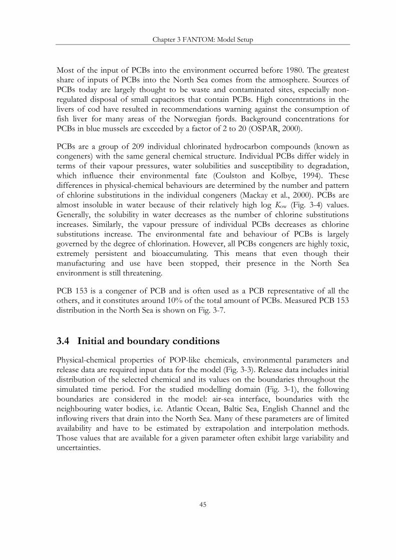
Chapter 3 FANTOM: Model Setup
45
Most of the input of PCBs into the environment occurred before 1980. The greatest share of inputs of PCBs into the North Sea comes from the atmosphere. Sources of PCBs today are largely thought to be waste and contaminated sites, especially non-regulated disposal of small capacitors that contain PCBs. High concentrations in the livers of cod have resulted in recommendations warning against the consumption of fish liver for many areas of the Norwegian fjords. Background concentrations for PCBs in blue mussels are exceeded by a factor of 2 to 20 (OSPAR, 2000).
PCBs are a group of 209 individual chlorinated hydrocarbon compounds (known as congeners) with the same general chemical structure. Individual PCBs differ widely in terms of their vapour pressures, water solubilities and susceptibility to degradation, which influence their environmental fate (Coulston and Kolbye, 1994). These differences in physical-chemical behaviours are determined by the number and pattern of chlorine substitutions in the individual congeners (Mackay et al., 2000). PCBs are almost insoluble in water because of their relatively high log Kow (Fig. 3-4) values. Generally, the solubility in water decreases as the number of chlorine substitutions increases. Similarly, the vapour pressure of individual PCBs decreases as chlorine substitutions increase. The environmental fate and behaviour of PCBs is largely governed by the degree of chlorination. However, all PCBs congeners are highly toxic, extremely persistent and bioaccumulating. This means that even though their manufacturing and use have been stopped, their presence in the North Sea environment is still threatening.
PCB 153 is a congener of PCB and is often used as a PCB representative of all the others, and it constitutes around 10% of the total amount of PCBs. Measured PCB 153 distribution in the North Sea is shown on Fig. 3-7.
3.4 Initial and boundary conditions Physical-chemical properties of POP-like chemicals, environmental parameters and release data are required input data for the model (Fig. 3-3). Release data includes initial distribution of the selected chemical and its values on the boundaries throughout the simulated time period. For the studied modelling domain (Fig. 3-1), the following boundaries are considered in the model: air-sea interface, boundaries with the neighbouring water bodies, i.e. Atlantic Ocean, Baltic Sea, English Channel and the inflowing rivers that drain into the North Sea. Many of these parameters are of limited availability and have to be estimated by extrapolation and interpolation methods. Those values that are available for a given parameter often exhibit large variability and uncertainties.

Chapter 3 FANTOM: Model Setup
46
Daily mean distributions of flow velocity components, their variances, sea surface height, diffusion coefficients, salinity and sea temperature were obtained from the corresponded HAMSOM simulations (Sect. 3.2).
Compound specific physical-chemical properties and degradation rates in seas water are taken from Klöpffer and Schmidt, (2001), Semeena and Lammel (2005) and Sahsuvar et al. (2003) and are listed in Table A-1.
The influence of sources outside the model domain is taken into account by using measurements data.
3.4.1 Initialisation
Initial distribution of POPs concentrations and their values on the sea boundaries were interpolated based on non-filtered samples (Theobald et al., 1996) and therefore represent the total concentration (dissolved and particle-bound). Initial conditions for the concentration are defined by the function 0C :
3-1
Initial distributions of γ-HCH, α-HCH and PCB 153 are shown on Fig. 3-5, 3-6 and Fig. 3-7 respectively.
3.4.2 Oceanic boundary conditions
The oceanic boundary values of POPs concentrations at the North Atlantic, Baltic Sea and the English Channel boundaries are extrapolated from the measured values used for the initialisation. Boundary conditions for the water boundaries B are prescribed:
3-2
where BC is the concentration at the water boundary. The boundary condition at the coast reads:
3-3
At the bottom, with the bottom depth H the tracer flux is:
3-4
( ) ( )zyxCzyxC ,,0,,, 0=
( )tzyxCC BBzyx ,,,),,( =∈
0),,( =∂∂
Γ∈zyxnC
setFF Hz ==

Chapter 3 FANTOM: Model Setup
47
The settling flux setF is calculated according to Eq. (2-14).
3.4.3 River loads
River input is a significant source for some POPs in the North Sea. The river loads of the selected chemicals in FANTOM from the European continental rivers including the Elbe, the Weser, the Ems, the Rhine and Meuse, and the Scheldt (Fig. 3-1) are calculated as a product of the daily fresh water discharge rivQ (m3 s-1) (Lenhart and Pätsch, 2004) and the concentrations of the compound at the last tidal gauge station of each river rivC (ng l-1) (Fig. 3-8b, Fig. 3-9b and Fig. 3-10b). Data for rivC from the German rivers provided by the corresponded Environmental Agencies were used. The pollutant concentrations in the Dutch rivers are available from the Dutch database DONAR. The loads of POPs reported to OSPAR (2000) were used for the Thames and the Humber. Values of rivC are available with different temporal resolutions, e.g. monthly means and have to be interpolated to fit the temporal resolution of the model.
3.4.4 Atmospheric boundary conditions
Boundary conditions at the air-sea interface are based on measured concentrations of POPs in the air and in precipitation (Fig. 3-3) available through the EMEP monitoring programme. The precipitation intensity is calculated using the ECMWF ERA-40 data. The measured values from several EMEP stations (Fig. 3-1) were interpolated to the whole domain. The tracer’s flux on the sea surface is determined as:
3-5
The flux surfF is calculated according to Eq. (2-2). Atmospheric data are discussed in Sect. 3.4.5.
3.4.5 Data compilation and quality
Because many model input parameters are of limited availability they have to be estimated by extrapolation and interpolation methods. Those values that are available for a given parameter often exhibit large variability and uncertainties. Monthly mean atmospheric concentrations used in this study for all three substances were those from the EMEP network (EMEP, 2005). Concentrations in the rivers were available with different temporal resolution: monthly means for the rivers Ems and Weser and weekly or bi-weekly for the other rivers.
surf0 FF z ==
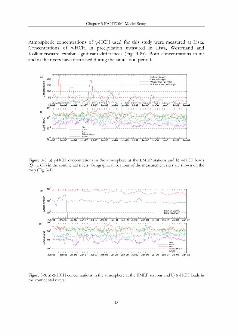
Chapter 3 FANTOM: Model Setup
48
Atmospheric concentrations of γ-HCH used for this study were measured at Lista. Concentrations of γ-HCH in precipitation measured in Lista, Westerland and Kollumerwaard exhibit significant differences (Fig. 3-8a). Both concentrations in air and in the rivers have decreased during the simulation period.
10
-4
10-2
100
102
Load
(mg/
s)
0
50
100
150
200
Con
cent
ratio
n
Jan-96 Jul-96 Jan-97 Jul-97 Jan-98 Jul-98 Jan-99 Jul-99 Jan-00 Jul-00 Jan-01 Jul-01 Jun-95 Jan-02
ElbeWeserEmsRhine & MeuseScheldt
Lista, air (pg/m3)Lista, rain (ng/l)Westerland, rain (ng/l)Kollumerw aard, rain (ng/l)
Jan-96 Jul-96 Jan-97 Jul-97 Jan-98 Jul-98 Jan-99 Jul-99 Jan-00 Jul-00 Jan-01 Jul-01 Jun-95 Jan-02
Jan-96 Jul-96 Jan-97 Jul-97 Jan-98 Jul-98 Jan-99 Jul-99 Jan-00 Jul-00 Jan-01 Jul-01 Jun-95 Jan-02
(a)
(b)
Figure 3-8: a) γ-HCH concentrations in the atmosphere at the EMEP stations and b) γ-HCH loads (Qriv x Criv) in the continental rivers. Geographical locations of the measurement sites are shown on the map (Fig. 3-1).
102
100
10-2
10-4
Load
(mg/
s)
10-2
100
102
Con
cent
ratio
n
ElbeWeserEmsRhine & MeuseScheldt
Lista, air (pg/m3)Lista, rain (ng/l)
Jan-96 Jul-96 Jan-97 Jul-97 Jan-98 Jul-98 Jan-99 Jul-99 Jan-00 Jul-00 Jan-01 Jul-01 Jun-95 Jan-02
Jan-96 Jul-96 Jan-97 Jul-97 Jan-98 Jul-98 Jan-99 Jul-99 Jan-00 Jul-00 Jan-01 Jul-01 Jun-95 Jan-02
(a)
(b)
Figure 3-9: a) α-HCH concentrations in the atmosphere at the EMEP stations and b) α-HCH loads in the continental rivers.

Chapter 3 FANTOM: Model Setup
49
Atmospheric concentrations and river loads of α-HCH and PCB 153 and river loads of γ-HCH exhibit large differences and therefore are presented on a logarithmic scale. Measured atmospheric concentrations of α-HCH and PCB 153 were available only at Lista between 1995 and 2001 (Fig. 3-9 and Fig. 3-10).
Air concentrations of α-HCH measured at Lista decreased, whereas concentrations in precipitations remained more or less at the same level (EMEP, 2005).
Concentrations of PCB 153 in the rain had slightly decreased in the end of 2001. In general, PCB 153 levels in the rivers and in air do not show any trend within the studied time period.
10-4
10-2
100
Load
(mg/
s)
10
-4
10-2
100
Con
cent
ratio
n
Lista, air (pg/m3)Lista, rain (ng/l)
ElbeWeserEmsRhine & MeuseScheldt
Jan-96 Jul-96 Jan-97 Jul-97 Jan-98 Jul-98 Jan-99 Jul-99 Jan-00 Jul-00 Jan-01 Jul-01 Jun-95 Jan-02
Jan-96 Jul-96 Jan-97 Jul-97 Jan-98 Jul-98 Jan-99 Jul-99 Jan-00 Jul-00 Jan-01 Jul-01 Jun-95 Jan-02
(a)
(b)
Figure 4-10: a) PCB 153 concentrations in the atmosphere at the EMEP stations and b) PCB 153 loads in the continental rivers.
Atmospheric concentrations of the three selected pollutants used for this study were measured at coastal stations. Therefore there is no information on possible concentration gradients over the whole North Sea and in the subregions remote from the polluted coastal areas. Concentrations of γ-HCH in precipitation measured in Lista, Westerland and Kollumerwaard exhibit significant differences (Fig. 3-8a). For some pollutants, air concentrations over the coastal waters are expected to be higher than those over the open ocean waters because of the proximity to sources. However, there are indications that air measured in Lista originate from the North Sea about 2/3 of the time (Haugen et al., 1998). Furthermore, measurements of atmospheric depositions of selected POPs in the Yellow Sea (Lammel et al., 2005) showed that gradients in air concentrations of “old” POPs over coastal waters are low. Since the measured air
Chapter 3 FANTOM: Model Setup
50
concentrations were available only from Lista they were used for the whole modelling domain.
Most of the data on the river loads of POPs are available through annual overviews which make a large number of them impossible to use for nowcast simulations. Measured atmospheric concentrations of POPs have a very poor spatial coverage and monitoring stations are located only along the coasts (Fig. 3-8b, Fig. 3-9b and Fig. 3-10b). This can introduce additional uncertainties into the model.

Chapter 4 FANTOM: Model Evaluation
51
Chapter 4
FANTOM: Model Evaluation
Model evaluation for the three compounds is presented in this chapter. Evaluation was preformed by comparing model results with available measurements of these POPs in sea water over the period of simulation. Data used for evaluation is shown in Section 4.1. Model evaluation for γ-HCH as well as for α-HCH and PCB 153 consisted of two stages.
(a) Calculated concentrations in sea water were compared with the measured ones (Sect. 4.2, Sect. 4-3 and Sect. 4-4). Locations of the measurement sites are shown on the Fig. 4-1.
(b) Model sensitivity to input parameters was analysed (Sect. 4-5).
4.1 Data used for model evaluation
Although PCB 153 and α- and γ-HCHs are rather well studied contaminants and subjects to national and international monitoring programmes, data availability remains an important constraint for constructing an observations based, spatially resolved model. Unlike regular monitoring in the atmosphere, where monthly or even weekly measurements of these contaminants are available for the European region (e.g. EMEP), observations of sea water concentrations are discrete in time and space due to operational constraints. This is illustrated by Table B-1 where geographical locations of available stations, number of measurements for α-, γ-HCHs and PCB 153 and months when the sampling was made are listed. Measurements for PCB 153 were not available at the location N, O and P (Dutch EEZ) for the studied period. Furthermore, out of the three substances considered in this study, data on PCB 153 are the scarcest.
Time series for observed γ-HCH concentrations in sea water covering the simulation period were available in 18 locations (Fig. 4-1). Most of the data were provided by the

Chapter 4 FANTOM: Model Evaluation
52
German Oceanographic Data Centre (DOD, 2005) covering only the German exclusive economic zone (EEZ) of the North Sea. Time series at locations N, O and P are from Dutch EEZ of the North Sea provided by the Dutch database Waterbase (DONAR, 2005).
At most of the locations, namely at A, G to P, measurements were made during warm seasons (May–September) corresponding to the predicted maxima (Table B-1). At locations B, C, D and F measurements were conducted between November and February.
AB
C
L
M
H GI
N
K
O
P
J
D
EF
Westerland
Lista (58.1oN, 6.5oE)
HaringvlietScheldt
Nieuw e Waterw eg
Nordzeekanaal
Kollumerw aard
Ijssel
Ems WeserElbe
Thames
Humber
Tyne
Forth
Welland
Tees
-2 0 2 4 6 851
52
53
54
55
56
57
Figure 4-1: FANTOM modelling domain and geographical locations of points where observation time series were available for the model evaluation (labelled with letters). Data for points A to M were provided by the German Oceanographic Centre (DOD, 2005) covering only the German exclusive economic zone of the North Sea. Data for points P, N and O are from the Dutch database Waterbase (DONAR, 2005). Stations where measurements of γ-HCH, α-HCH and PCB 153 atmospheric concentrations were available are indicated in red (Lista lies outside of the modelling domain). Rivers mouths are indicated in green.

Chapter 4 FANTOM: Model Evaluation
53
4.2 Comparison between modelled and measured sea water concentrations of γ-HCH Daily averaged concentrations in the uppermost sea layer were compared with the individual measurements and plotted for some points (Fig. 4-2) located in different subregions of the North Sea and with sufficient number of measurements (Fig. 4-1).
A clear seasonal pattern with higher concentrations in summer is predicted for most years in all locations. Similar patterns are also found in the atmospheric concentrations (Fig. 3-8a) and in the continental river loads of γ-HCH (Fig. 3-8b). The highest concentrations, up to 3.95 ng l-1 (Table 4-1), were found at locations near the coast, e.g. A (Fig. 4-12a), G and K (Fig. 4-2b and Fig.4-3d); the lowest ones, of less than 0.2 ng l-1 (Table 4-1), were found in the open North Sea at locations L and P (Fig. 4-3b and c).
Table 4-1: Stations used for the model results evaluation for γ-HCH, mean and range of measurements and model results and correlation coefficients between measurements and model results.
Symbol on the map
Measurements: mean and range (ng/l)
Model results: mean and range (ng/l)
Correlation coefficient
A 1.50 (0.37 – 3.00) 1.48 (0.58 – 3.03) 0.95
B 0.70 (0.10 – 3.00) 1.41 (0.81 – 2.24) 0.35
C 0.83 (0.10 – 3.00) 1.27 (0.68 – 1.88) 0.40
D 0.80 (0.10 – 2.00) 1.32 (0.69 – 1.32) 0.30
E 1.86 (0.10 – 3.00) 1.32 (0.67 – 2.47) 0.74
F 0.82 (0.10 – 2.00) 1.08 (0.62 – 1.52) 0.23
G 1.65 (0.43 – 3.95) 1.77 (0.86 – 3.00) 0.77
H 1.63 (0.42 – 2.55) 1.19 (0.68 – 1.76) 0.93
I 1.45 (0.30 – 3.49) 0.95 (0.38 – 1.31) 0.77
J 0.71 (0.23 – 1.32) 0.67 (0.35 – 1.23) 0.84
K 1.25 (0.42 – 2.75) 1.50 (0.74 – 2.33) 0.86
L 0.58 (0.17 – 0.95) 0.58 (0.22 – 0.91) 0.84
M 0.42 (0.28 – 0.70) 0.49 (0.38 – 0.59) 0.45
N 0.79 (0.20 – 1.80) 1.00 (0.63 – 1.51) 0.83
O 1.25 (0.50 – 0.70) 1.08 (0.96 – 1.15) 0.68
P 0.72 (0.10 – 1.20) 0.67 (0.32 – 1.07) 0.94
Q 1.16 (0.70 – 1.41) 0.96 (0.45 – 1.17) 0.93
R 0.80 (0.45 – 1.26) 1.06 (0.73 – 1.41) 0.92
Average 1.05 (0.28 – 2.29) 1.11 (0.64 – 1.67) 0.68

Chapter 4 FANTOM: Model Evaluation
54
0
1
2
3
4
Con
cent
ratio
n (n
g/l)
Jan-96 Jul-96 Jan-97 Jul-97 Jan-98 Jul-98 Jan-99 Jul-99 Jan-00 Jul-00 Jan-01 Jul-01 Jun-95 Jan-02
0
1
2
3
4
Con
cent
ratio
n (n
g/l)
Jan-96 Jul-96 Jan-97 Jul-97 Jan-98 Jul-98 Jan-99 Jul-99 Jan-00 Jul-00 Jan-01 Jul-01 Jun-95 Jan-02
0
1
2
3
4
Con
cent
ratio
n (n
g/l)
Jan-96 Jul-96 Jan-97 Jul-97 Jan-98 Jul-98 Jan-99 Jul-99 Jan-00 Jul-00 Jan-01 Jul-01 Jun-95 Jan-02
0
1
2
3
4
Con
cent
ratio
n (n
g/l)
Jan-96 Jul-96 Jan-97 Jul-97 Jan-98 Jul-98 Jan-99 Jul-99 Jan-00 Jul-00 Jan-01 Jul-01 Jun-95 Jan-02
modelobservations
modelobservations
modelobservations
modelobservations
D
G
H
F
(a)
(b)
(c)
(d)
Figure 4-2: Observed (dots) and calculated by FANTOM (solid line) γ-HCH concentrations (ng/l) in the surface layer at the locations D, G, H, F. Geographical locations of points are given in Table B-1 and shown on Fig. 4-1.

Chapter 4 FANTOM: Model Evaluation
55
0
0.5
1
1.5
2
Con
cent
ratio
n (n
g/l)
Jan-96 Jul-96 Jan-97 Jul-97 Jan-98 Jul-98 Jan-99 Jul-99 Jan-00 Jul-00 Jan-01 Jul-01 Jun-95 Jan-02
0
0.5
1
1.5
2
Con
cent
ratio
n (n
g/l)
Jan-96 Jul-96 Jan-97 Jul-97 Jan-98 Jul-98 Jan-99 Jul-99 Jan-00 Jul-00 Jan-01 Jul-01 Jun-95 Jan-02
0
1
2
3
4
Con
cent
ratio
n (n
g/l)
Jan-96 Jul-96 Jan-97 Jul-97 Jan-98 Jul-98 Jan-99 Jul-99 Jan-00 Jul-00 Jan-01 Jul-01 Jun-95 Jan-02
0
0.5
1
1.5
2
Con
cent
ratio
n (n
g/l)
Jan-96 Jul-96 Jan-97 Jul-97 Jan-98 Jul-98 Jan-99 Jul-99 Jan-00 Jul-00 Jan-01 Jul-01 Jun-95 Jan-02
modelobservations
modelobservations
modelobservations
modelobservations
J
L
P
K
(a)
(b)
(c)
(d)
Figure 4-3: Observed (dots) and calculated by FANTOM (solid line) γ-HCH concentrations (ng/l) in the surface layer at the locations J, L, P, K. Geographical locations of points are given in Table B-1 and shown on Fig. 4-1.

Chapter 4 FANTOM: Model Evaluation
56
Concentration of γ-HCH had decreased in all locations throughout the simulation period. The biggest drop in γ-HCH concentrations, 6–7 times, was found in the German Bight, with the smallest, 3–4 times, in the central North Sea. Both observed and modelled concentrations in sea water at all locations increased during the first half of the simulation period, with highest concentrations in 1997–1998. During the second half of the simulation, in the years 1998–2001, there are negative trends in concentrations at all locations, both in observations and predictions by FANTOM. Also atmospheric concentrations of γ-HCH reflect such pattern with the highest concentrations of γ-HCH detected in precipitation during spring and summer of 1997 and decreased concentrations during 1998-2001 (Fig. 3-8a).
Time series of γ-HCH concentration in the southern North Sea surface water reported elsewhere (SRU, 2004) show a gradual decrease since the 1982 due to the restriction in γ-HCH application in the countries adjacent the North Sea. This decrease is captured by the model during the studied period. Furthermore, model results suggest that γ-HCH concentrations declined in the entire modelling domain.
The jagged pattern in the concentration’s time series in the German Bight (Fig. 4-2 and Fig. 4-3) is due to variability of the fresh water inflow (Fig. 3-8b). As opposed to the German Bight, in the open North Sea (Fig. 4-3b, c) remote from the polluted estuaries, time series are smoother and sea water concentrations seem to be balanced by the volatilisation-deposition process.
No measurements of γ-HCH concentrations in the English Channel and on the northern sea boundary were available for this study. Since concentrations in the whole North Sea decreased they have probably also decreased in the English Channel and on the northern sea boundary without being captured by the model. This offers an explanation for the overestimations in calculated concentrations during the years 2000–2001. The overestimation is most pronounced at location N, lying in the passage of the English Channel water.
In order to evaluate the model results, measured γ-HCH concentrations are plotted against calculated ones in scatter plots for some locations (Fig. 4-4). Correlation coefficients for all locations where time series were available are presented in Table . Good correlation was found for locations A, B and P with correlation coefficients of 0.94, 0.93 and 0.94 respectively. Lower correlation coefficients between 0.23 and 0.40 were found for the locations F, D, B and C where the time series consist of the measurements conducted between December and March. The number of measurements and their temporal resolution, in particular at the locations P, O and M, make further statistical analysis inappropriate.

Chapter 4 FANTOM: Model Evaluation
57
0 0.5 1 1.5 20
0.5
1
1.5
2
Mea
sure
d co
ncen
tratio
n (n
g/l)
Calculated concentration (ng/l)
N
0 0.2 0.4 0.6 0.8 1 1.2 1.40
0.2
0.4
0.6
0.8
1
1.2
1.4
Mea
sure
d co
ncen
tratio
n (n
g/l)
Calculated concentration (ng/l)
P
0 1 2 3 40
1
2
3
4
Calculated concentration (ng/l)
Mea
sure
d co
ncen
tratio
n (n
g/l) G
0 0.5 1 1.5 2 2.5 3 3.50
0.5
1
1.5
2
2.5
3
3.5
Calculated concentration (ng/l)
Mea
sure
d co
ncen
tratio
n (n
g/l) A
0 0.5 1 1.5 2 2.5 30
0.5
1
1.5
2
2.5
3
Mea
sure
d co
ncen
tratio
n (n
g/l)
Calculated concentration (ng/l)
K
0 0.2 0.4 0.6 0.8 10
0.2
0.4
0.6
0.8
1
Mea
sure
d co
ncen
tratio
n (n
g/l)
Calculated concentration (ng/l)
L
(a) (b)
(c)
(e)
(d)
(f)
Figure 4-4: Measured vs. calculated γ-HCH concentrations (ng/l) in the surface layer at the locations A, G, K, L, N, P. Geographical locations of points are given in Table B-1 and shown on Figure 4-1.
Correlation coefficients calculated for locations B, C, D and F measured during colder season (Table 4-1) are lower, even though they are situated only within a few model grid points from locations A, E, G and H, where measurements were conducted during warmer seasons and where correlations are much higher. Calculated mean concentrations at locations B, C, D and F are higher than observed (Table 4-1). One explanation for this discrepancy could be that during winter the stronger winds which
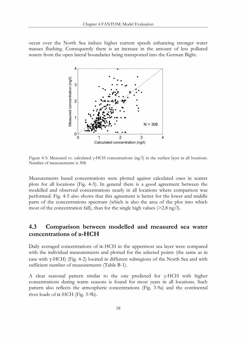
Chapter 4 FANTOM: Model Evaluation
58
occur over the North Sea induce higher current speeds enhancing stronger water masses flushing. Consequently there is an increase in the amount of less polluted waters from the open lateral boundaries being transported into the German Bight.
0 1 2 3 40
1
2
3
4
Calculated concentration (ng/l)
Mea
sure
d co
ncen
tratio
n (n
g/l)
N = 308
Figure 4-5: Measured vs. calculated γ-HCH concentrations (ng/l) in the surface layer in all locations. Number of measurements is 308.
Measurements based concentrations were plotted against calculated ones in scatter plots for all locations (Fig. 4-5). In general there is a good agreement between the modelled and observed concentrations nearly in all locations where comparison was performed. Fig. 4-5 also shows that this agreement is better for the lower and middle parts of the concentrations spectrum (which is also the area of the plot into which most of the concentration fall), than for the single high values (>2.8 ng/l).
4.3 Comparison between modelled and measured sea water concentrations of α-HCH
Daily averaged concentrations of α-HCH in the uppermost sea layer were compared with the individual measurements and plotted for the selected points (the same as in case with γ-HCH) (Fig. 4-2) located in different subregions of the North Sea and with sufficient number of measurements (Table B-1).
A clear seasonal pattern similar to the one predicted for γ-HCH with higher concentrations during warm seasons is found for most years in all locations. Such pattern also reflects the atmospheric concentrations (Fig. 3-9a) and the continental river loads of α-HCH (Fig. 3-9b).

Chapter 4 FANTOM: Model Evaluation
59
Table 4-2: Stations used for the model results evaluation for α-HCH, mean and range of measurements and model results and correlation coefficients between measurements and model results.
Symbol on the map
Model results: mean and range (ng/l)
Measurements: mean and range (ng/l)
Correlation coefficient
A 0.28 (0.18 – 0.46) 0.23 (0.075 – 0.65) 0.75
B 0.31 (0.17 – 0.50) 0.26 (0.04 – 1) 0.51
C 0.34 (0.20 – 0.68) 0.43 (0.07 – 1) 0.27
D 0.34 (0.20 –0.70) 0.40 (0.04 – 2) 0.07
E 0.35 (0.19 – 0.76) 0.31 (0.04 – 1) 0.20
F 0.16 (0.27 –0.42) 0.40 (0.07 – 1) 0.05
G 0.46 (0.22 – 0.79) 0.46 (0.14 – 2) 0.38
H 0.27 (0.12 – 0.40) 0.22 (0.07 – 0.53) 0.81
I 0.25 (0.11 – 0.34) 0.20 (0.07 – 0.44) 0.68
J 0.22 (0.11 – 0.33) 0.19 (0.07 – 0.30) 0.85
K 0.30 (0.19 – 0.44) 0.26 (0.12 –0.63) 0.80
L 0.19 (0.08 – 0.33) 0.23 (0.09 – 0.38) 0.79
N 0.14 (0.04 – 0.25) 0.13 (0.10 – 0.30) 0.64
O 0.13 (0.10 – 0.18) 0.13 (0.10 – 0.30) 0.52
P 0.20 (0.12 – 0.32) 0.16 (0.10 – 0.30) 0.90
Q 0.20 (0.13 – 0.33) 0.15 (0.08 – 0.26) 0.91
R 0.23 (0.18 – 0.27) 0.16 (0.10 – 0.23) 0.24
Average 0.26 (0.14 – 0.43) 0.23 (0.08 – 0.70) 0.43
The highest concentrations, up to 0.7 ng l-1 (Table 4-2), were predicted by the model at locations near the coast, e.g. A (Fig. 4-13a) and K (Fig. 4-7d). Also concentrations measured in the River Elbe were very high (up to 5 ng l-1) in August 1995 indicating that it is still a considerable source of α-HCH. The lowest concentrations, of less than 0.1 ng l-1 (Table 4-2), were predicted in the open North Sea at locations L and P (Fig. 4-7b and c).
The calculated concentrations values are in a good agreement with those from monitoring programs carried out during the same period. Concentration of α-HCH had decreased in all locations throughout the simulation period. However, unlike γ-HCH concentrations, α-HCH concentrations dropped more or less homogeneously in the entire modelling domain indicating the local sources of α-HCH are probably less significant in the entire North Sea than those for γ-HCH. Other studies also show that following the ban on technical HCH, there is an ongoing decrease of α-HCH concentrations in the North Sea detected since 1982 (Theobald et al., 1996; Bethan et al., 2001; OSPAR, 2000; SRU, 2005).
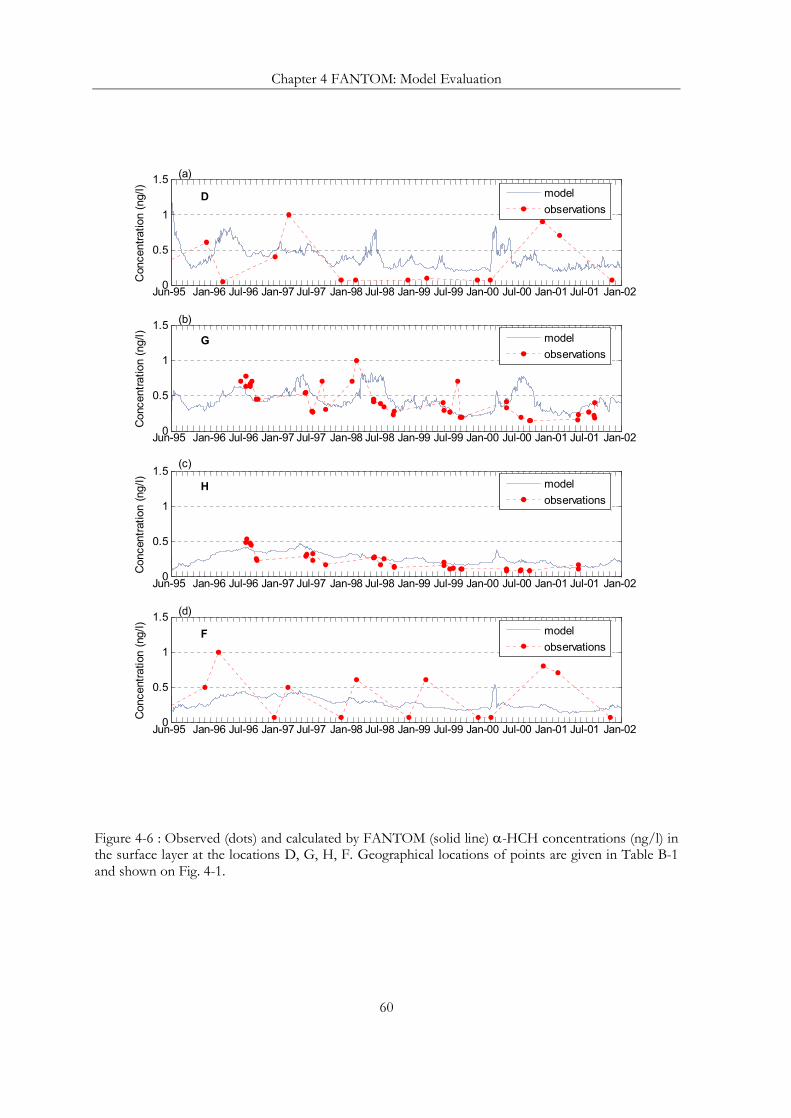
Chapter 4 FANTOM: Model Evaluation
60
0
0.5
1
1.5
Con
cent
ratio
n (n
g/l)
Jan-96 Jul-96 Jan-97 Jul-97 Jan-98 Jul-98 Jan-99 Jul-99 Jan-00 Jul-00 Jan-01 Jul-01 Jun-95 Jan-02
0
0.5
1
1.5
Con
cent
ratio
n (n
g/l)
Jan-96 Jul-96 Jan-97 Jul-97 Jan-98 Jul-98 Jan-99 Jul-99 Jan-00 Jul-00 Jan-01 Jul-01 Jun-95 Jan-02
0
0.5
1
1.5
Con
cent
ratio
n (n
g/l)
Jan-96 Jul-96 Jan-97 Jul-97 Jan-98 Jul-98 Jan-99 Jul-99 Jan-00 Jul-00 Jan-01 Jul-01 Jun-95 Jan-02
0
0.5
1
1.5
Con
cent
ratio
n (n
g/l)
Jan-96 Jul-96 Jan-97 Jul-97 Jan-98 Jul-98 Jan-99 Jul-99 Jan-00 Jul-00 Jan-01 Jul-01 Jun-95 Jan-02
modelobservations
modelobservations
modelobservations
modelobservations
D
G
H
F
(a)
(b)
(c)
(d)
Figure 4-6 : Observed (dots) and calculated by FANTOM (solid line) α-HCH concentrations (ng/l) in the surface layer at the locations D, G, H, F. Geographical locations of points are given in Table B-1 and shown on Fig. 4-1.

Chapter 4 FANTOM: Model Evaluation
61
0
0.1
0.2
0.3
0.4
Con
cent
ratio
n (n
g/l)
Jan-96 Jul-96 Jan-97 Jul-97 Jan-98 Jul-98 Jan-99 Jul-99 Jan-00 Jul-00 Jan-01 Jul-01 Jun-95 Jan-02
0
0.1
0.2
0.3
0.4
Con
cent
ratio
n (n
g/l)
Jan-96 Jul-96 Jan-97 Jul-97 Jan-98 Jul-98 Jan-99 Jul-99 Jan-00 Jul-00 Jan-01 Jul-01 Jun-95 Jan-02
0
0.1
0.2
0.3
0.4
Con
cent
ratio
n (n
g/l)
Jan-96 Jul-96 Jan-97 Jul-97 Jan-98 Jul-98 Jan-99 Jul-99 Jan-00 Jul-00 Jan-01 Jul-01 Jun-95 Jan-02
0
0.2
0.4
0.6
0.8
Con
cent
ratio
n (n
g/l)
Jan-96 Jul-96 Jan-97 Jul-97 Jan-98 Jul-98 Jan-99 Jul-99 Jan-00 Jul-00 Jan-01 Jul-01 Jun-95 Jan-02
modelobservations
modelobservations
modelobservations
modelobservations
J
L
P
K
(a)
(b)
(c)
(d)
Figure 4-7: Observed (dots) and calculated by FANTOM (solid line) α-HCH concentrations (ng/l) in the surface layer at the locations J, L, P, K. Geographical locations of points are given in Table B-1 and shown on Fig. 4-1.
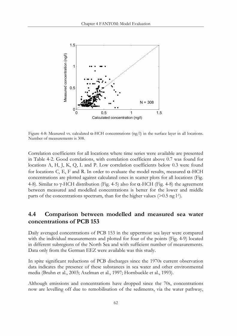
Chapter 4 FANTOM: Model Evaluation
62
0 0.5 1 1.50
0.5
1
1.5
Calculated concentration (ng/l)
Mea
sure
d co
ncen
tratio
n (n
g/l)
N = 308
Figure 4-8: Measured vs. calculated α-HCH concentrations (ng/l) in the surface layer in all locations. Number of measurements is 308.
Correlation coefficients for all locations where time series were available are presented in Table 4-2. Good correlations, with correlation coefficient above 0.7 was found for locations A, H, J, K, Q, L and P. Low correlation coefficients below 0.3 were found for locations C, E, F and R. In order to evaluate the model results, measured α-HCH concentrations are plotted against calculated ones in scatter plots for all locations (Fig. 4-8). Similar to γ-HCH distribution (Fig. 4-5) also for α-HCH (Fig. 4-8) the agreement between measured and modelled concentrations is better for the lower and middle parts of the concentrations spectrum, than for the higher values (>0.5 ng l-1).
4.4 Comparison between modelled and measured sea water concentrations of PCB 153 Daily averaged concentrations of PCB 153 in the uppermost sea layer were compared with the individual measurements and plotted for four of the points (Fig. 4-9) located in different subregions of the North Sea and with sufficient number of measurements. Data only from the German EEZ were available was this study.
In spite significant reductions of PCB discharges since the 1970s current observation data indicates the presence of these substances in sea water and other environmental media (Bruhn et al., 2003; Axelman et al., 1997; Hornbuckle et al., 1993).
Although emissions and concentrations have dropped since the 70s, concentrations now are levelling off due to remobilisation of the sediments, via the water pathway,
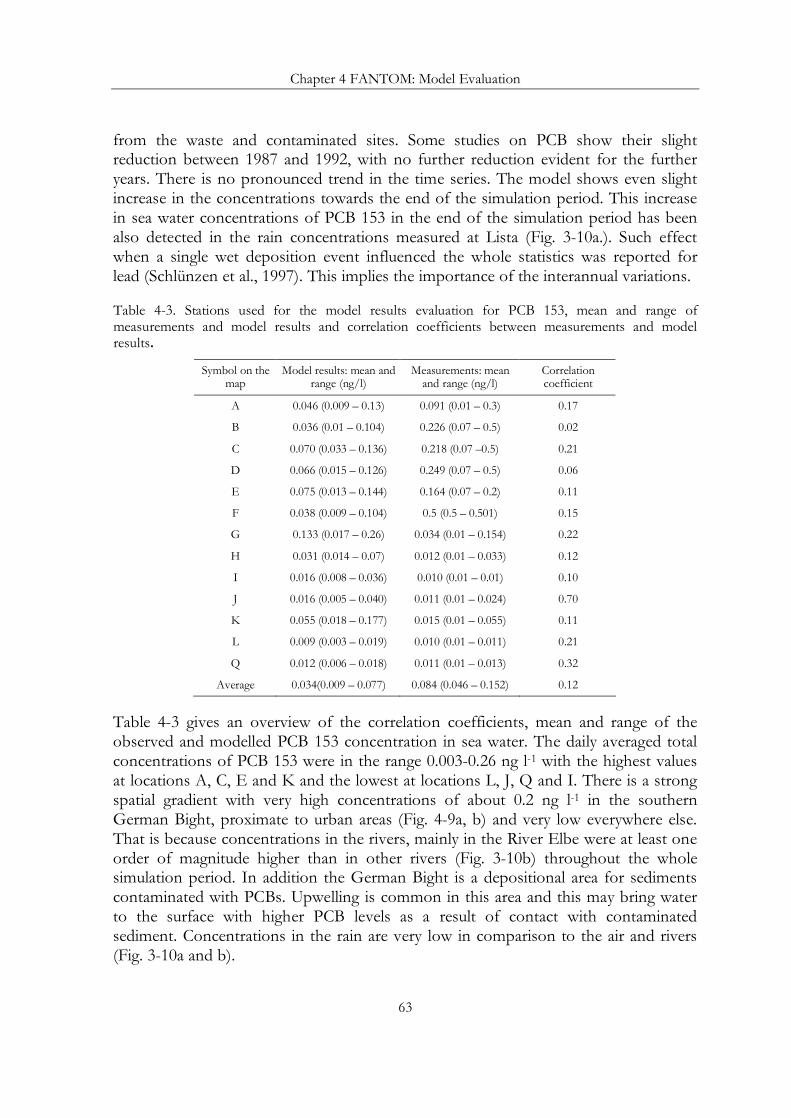
Chapter 4 FANTOM: Model Evaluation
63
from the waste and contaminated sites. Some studies on PCB show their slight reduction between 1987 and 1992, with no further reduction evident for the further years. There is no pronounced trend in the time series. The model shows even slight increase in the concentrations towards the end of the simulation period. This increase in sea water concentrations of PCB 153 in the end of the simulation period has been also detected in the rain concentrations measured at Lista (Fig. 3-10a.). Such effect when a single wet deposition event influenced the whole statistics was reported for lead (Schlünzen et al., 1997). This implies the importance of the interannual variations.
Table 4-3. Stations used for the model results evaluation for PCB 153, mean and range of measurements and model results and correlation coefficients between measurements and model results.
Symbol on the map
Model results: mean and range (ng/l)
Measurements: mean and range (ng/l)
Correlation coefficient
A 0.046 (0.009 – 0.13) 0.091 (0.01 – 0.3) 0.17
B 0.036 (0.01 – 0.104) 0.226 (0.07 – 0.5) 0.02
C 0.070 (0.033 – 0.136) 0.218 (0.07 –0.5) 0.21
D 0.066 (0.015 – 0.126) 0.249 (0.07 – 0.5) 0.06
E 0.075 (0.013 – 0.144) 0.164 (0.07 – 0.2) 0.11
F 0.038 (0.009 – 0.104) 0.5 (0.5 – 0.501) 0.15
G 0.133 (0.017 – 0.26) 0.034 (0.01 – 0.154) 0.22
H 0.031 (0.014 – 0.07) 0.012 (0.01 – 0.033) 0.12
I 0.016 (0.008 – 0.036) 0.010 (0.01 – 0.01) 0.10
J 0.016 (0.005 – 0.040) 0.011 (0.01 – 0.024) 0.70
K 0.055 (0.018 – 0.177) 0.015 (0.01 – 0.055) 0.11
L 0.009 (0.003 – 0.019) 0.010 (0.01 – 0.011) 0.21
Q 0.012 (0.006 – 0.018) 0.011 (0.01 – 0.013) 0.32
Average 0.034(0.009 – 0.077) 0.084 (0.046 – 0.152) 0.12
Table 4-3 gives an overview of the correlation coefficients, mean and range of the observed and modelled PCB 153 concentration in sea water. The daily averaged total concentrations of PCB 153 were in the range 0.003-0.26 ng l-1 with the highest values at locations A, C, E and K and the lowest at locations L, J, Q and I. There is a strong spatial gradient with very high concentrations of about 0.2 ng l-1 in the southern German Bight, proximate to urban areas (Fig. 4-9a, b) and very low everywhere else. That is because concentrations in the rivers, mainly in the River Elbe were at least one order of magnitude higher than in other rivers (Fig. 3-10b) throughout the whole simulation period. In addition the German Bight is a depositional area for sediments contaminated with PCBs. Upwelling is common in this area and this may bring water to the surface with higher PCB levels as a result of contact with contaminated sediment. Concentrations in the rain are very low in comparison to the air and rivers (Fig. 3-10a and b).

Chapter 4 FANTOM: Model Evaluation
64
0
0.05
0.1
0.15
0.2
Con
cent
ratio
n (n
g/l)
Jan-96 Jul-96 Jan-97 Jul-97 Jan-98 Jul-98 Jan-99 Jul-99 Jan-00 Jul-00 Jan-01 Jul-01 Jun-95 Jan-02
0
0.05
0.1
Con
cent
ratio
n (n
g/l)
Jan-96 Jul-96 Jan-97 Jul-97 Jan-98 Jul-98 Jan-99 Jul-99 Jan-00 Jul-00 Jan-01 Jul-01 Jun-95 Jan-02
0
0.05
0.1
Con
cent
ratio
n (n
g/l)
Jan-96 Jul-96 Jan-97 Jul-97 Jan-98 Jul-98 Jan-99 Jul-99 Jan-00 Jul-00 Jan-01 Jul-01 Jun-95 Jan-02
modelobservations
modelobservations
modelobservations
0
0.1
0.2
0.3
0.4
Con
cent
ratio
n (n
g/l)
Jan-96 Jul-96 Jan-97 Jul-97 Jan-98 Jul-98 Jan-99 Jul-99 Jan-00 Jul-00 Jan-01 Jul-01 Jun-95 Jan-02
modelobservations
A
H
J
L
(a)
(b)
(c)
(d)
Figure 4-9: Observed (dots) and calculated by FANTOM (solid line) PCB 153 total concentrations (ng/l) in the surface layer at the locations A, H, J, L. Geographical locations of points are given in Table B-1 and shown on Fig. 4-1.

Chapter 4 FANTOM: Model Evaluation
65
PCB 153 is the most hydrophobic compound among those addressed in this study. According to theoretical expectations more hydrophobic compounds will be exported with SPM downward out of the surface water more effectively than more hydrophilic substances. For the higher chlorinated PCBs, this process can be so efficient that the downward loss cannot be compensated by air-sea exchange, creating a fugacity deficit in the surface water (Dachs et al., 1999, 2002).
Wania et al., (2000) concluded that on average, volatilisation of PCBs exceeded gaseous deposition by a factor of 10 for the Baltic Sea. The differences in the calculated fluxes reported in the literature (Wania et al., 2000; Axelman et al, 2001; Bruhn et al., 2003) arise largely form the choice of the Henry’s law constant. The atmospheric particle bound deposition of PCBs to the Baltic reported in these studies was much greater while the gross gaseous deposition was much smaller. Therefore, it seems that as in case with HCHs the main uncertainty here is due to the choice of physical-chemical properties.
0 0.05 0.1 0.15 0.2 0.25 0.30
0.05
0.1
0.15
0.2
0.25
0.3
0.35
Calculated concentration (ng/l)
Mea
sure
d co
ncen
tratio
n (n
g/l)
N = 186
Figure 4-10: Measured vs. calculated PCB 153 concentrations (ng/l) in the surface layer in all locations. Number of measurements is 186.
Modelled PCB 153 concentrations are plotted against calculated ones in scatter plots for all locations (Fig. 4-10). Correlation coefficients for all locations where time series were available are presented in Table 4-3. Best correlation for PCB 153 was found for location J correlation coefficient of 0.7. Low correlation coefficients between 0.1 and 0.3 were found in most of the locations.
Due to low concentration of PCB 153 in sea water and the potential for shipboard as well as laboratory contamination, its analytical data is the most uncertain and often lie below the detection limit (BSH, 2005.). This problem is demonstrated by Fig. 4-9b, c, d

Chapter 4 FANTOM: Model Evaluation
66
and Fig. 4-10. At many locations measured concentrations remained constant (at the detection limit) throughout the simulation period (Fig. 4-10), whereas modelled concentration time series mirror variability in the input data. To illustrate this phenomenon modelled and measured concentrations at the location E close to the River Elbe mouth were compared with the supplement concentration from the River Elbe (Fig. 4-11). Although the values of both measured and modelled concentration lie in the same range, the concentration pattern is not reproduced. In fact the modelled concentration at this location is influenced by the River Elbe inflow which is also calculated using daily measurements data on the fresh water discharge and PCB 153 concentrations in the Elbe (see Sect. 3.4.3).
0
0.1
0.2
0.3
0.4
Con
cent
ratio
n (n
g/l)
Jan-96 Jul-96 Jan-97 Jul-97 Jan-98 Jul-98 Jan-99 Jul-99 Jan-00 Jul-00 Jan-01 Jul-01 Jan-02 Jun-95
observations at the location Emodel: at the location Esupplement from the Elbe
Figure 4-11: Concentrations of PCB 153: blue line – model simulation in the German Bight at the location E; green – concentration supplement form the River Elbe; red – individual measurements at the location E.
Unlike the two HCH isomers presented in the above sections there is no clear annual signal detected in the concentration time series. Other authors have also found the seasonal variability of gaseous PCB concentrations at marine stations in the southern Baltic Sea to be less than an order of magnitude (Bruhn et al., 2003; Agrell et al., 1999).
Concentrations of PCB 153 in the North Sea appear to be stabilising at lower levels as a result of its declining use since the 1970s (SRU, 2005). This is reproduced by the model. No pronounced seasonal trend is detected in the modelled PCB 153 concentrations. In general, the modelled PCB 153 concentrations are in the same range with respect to observations. However the agreement between measure and modelled concentration patterns is rather poor. This is probably due to both the model uncertainties and the measured data uncertainties.

Chapter 4 FANTOM: Model Evaluation
67
4.5 Uncertainty and sensitivity analysis
Since data from field studies are scarce, quantitative comparison of model results with measured data is difficult. Therefore sensitivity and uncertainty analyses as well as model comparison studies are important means for the evaluation of the model. The uncertainty in the modelling results is introduced by the uncertainties in the:
(a) input data based on field studies (see Sect. 3.4);
(b) substance properties, i.e. physical-chemical properties and degradation rates (Sect. 3.3);
(c) assumptions made in the model connected to the lack of some processes understanding (e.g. see Sect. 2.1).
The input data is discussed in Sect. 3.3. The observational data are scarce. Therefore, it is difficult to obtain quantitative estimates of the input data uncertainties connected to the sampling and analysis methods and data reporting.
As for the source of uncertainties mentioned under point (c), caused by the model formulation and simplification of processes, the sensitivity studies should be aimed at distinguishing the relative importance of one or another process. Such experiments are performed and discussed in Chapter 6.
To evaluate the assumptions made under point (a) and (b) experiments aimed at explaining the deviations in modelled and observed γ-HCH concentrations were performed (Fig. 4-12). In the first experiment it was assumed that the concentration of γ-HCH in water flowing into the North Sea from the English Channel and from the Atlantic Ocean at the northern boundary of the modelling domain is zero, i.e. 0B =C (Eq. 3-2). The resulting time series of the concentration was plotted for location A in the German Bight where the impact of inflow from lateral boundaries was expected to be less pronounced than elsewhere and for the location N lying in the passage of waters flowing from the English Channel. In the second experiment the Henry’s law constant temperature dependency (Eq. 2-7) was calculated using the values obtained by Kucklick et al. (1991) instead of those by Sahsuvar et al. (2003) used in other model runs (Table A-1). Daily averaged concentrations in the uppermost sea layer resulting from the main simulation and both experiments were compared with the individual measurements at the locations A and N (Fig. 4-12).

Chapter 4 FANTOM: Model Evaluation
68
0
0.5
1
1.5
2
2.5
Con
cent
ratio
n (n
g/l)
Jan-96 Jul-96 Jan-97 Jul-97 Jan-98 Jul-98 Jan-99 Jul-99 Jan-00 Jul-00 Jan-01 Jul-01 Jan-02 Jun-95
observationsmodel main simulationmodel: Hc(Tw ) after Kucklick (1991)
model: no Engl. Channel & Atlantic inflow
N
0
0.5
1
1.5
2
2.5
3
3.5C
once
ntra
tion
(ng/
l)
Jan-96 Jul-96 Jan-97 Jul-97 Jan-98 Jul-98 Jan-99 Jul-99 Jan-00 Jul-00 Jan-01 Jul-01 Jan-02 Jun-95
observationsmodel main simulationmodel: Hc(Tw ) after Kucklick (1991)
model: no Engl. Channel & Atlantic inflow
A(a)
(b)
Figure 4-12: Observed (dots) and calculated by FANTOM (solid lines) γ-HCH concentrations (ng/l) in the surface layer at the location A and N, under different model setup: blue line – main model simulation; magenta line – when γ-HCH concentrations inflowing via the lateral boundaries were equal zero; green – when air-sea exchange was calculated using Henry’s law constants given by Kucklick et al. (1991). Geographical location is given in Table B-1 and shown on Fig. 4-1.
As mentioned above the decrease in γ-HCH concentrations in the English Channel and on the northern boundary might not be correctly captured by the model leading to overestimated winter concentrations. This hypothesis is verified by the modelling experiment when γ-HCH concentrations in the English Channel and on the northern boundary of the modelling domain were set to zero for the entire simulation period. Fig. 4-12 shows that concentration without inflow from the lateral boundaries was a significant component of the γ-HCH burden until the second half of the year 2000. Fig. 4-12 also suggests that this effect is more pronounced in winter than in summer. This is confirmed by the correlation coefficients (Table 4-1). Furthermore, ongoing cycling of earlier emitted γ-HCH leakages from inappropriate disposal may play a role.

Chapter 4 FANTOM: Model Evaluation
69
0
0.1
0.2
0.3
0.4
0.5
0.6
0.7
0.8C
once
ntra
tion
(ng/
l)
Jan-96 Jul-96 Jan-97 Jul-97 Jan-98 Jul-98 Jan-99 Jul-99 Jan-00 Jul-00 Jan-01 Jul-01 Jan-02 Jun-95
observationsmodel: main simulationmodel: Hc(Tw ) after Sachsuvar (2003)
model: no Engl. Channel & Atlantic inflow
A(a)
0
0.1
0.2
0.3
0.4
0.5
0.6
0.7
0.8
Con
cent
ratio
n (n
g/l)
Jan-96 Jul-96 Jan-97 Jul-97 Jan-98 Jul-98 Jan-99 Jul-99 Jan-00 Jul-00 Jan-01 Jul-01 Jan-02 Jun-95
observationsmodel: main simulationmodel: Hc(Tw ) after Sahsuvar (2003)
model: no Engl. Channel & Atlantic inflow
N(b)
Figure 4-13: Observed (dots) and calculated by FANTOM (solid lines) α-HCH concentrations (ng/l) in the surface layer at the location A and N, under different model setup: blue line – main model simulation; magenta line – when α-HCH concentrations inflowing via the lateral boundaries were equal zero; green – when air-sea exchange was calculated using Henry’s law constants given by Sahsuvar et al. (2003). Geographical location is given in Table B-1 and shown on Fig. 4-1.
The seasonal pattern predicted by the model with higher γ-HCH concentrations during summer than during winter emphasises the importance of temperature dependency of the air-sea exchange. For the Great Lakes and for the Arctic Ocean it has been found that during summer, the air-sea gas transfer is net volatilisational, whereas during colder period it is depositional (Ridal et al., 1996; Jantunen and Bidleman, 1997). Measurements suggest (Sahsuvar et al., 2003) that temperature dependency of cH has a profound effect on gas exchange predictions. This hypothesis is also illustrated by Fig. 4-12 where γ-HCH concentrations resulting from model calculations using two

Chapter 4 FANTOM: Model Evaluation
70
different temperature dependency coefficients of cH is presented. This experiment shows that most recent data (Sahsuvar et al., 2003) lead to higher (20-50%) sea water concentrations. Therefore, as parameterisation of the air-sea exchange seems to play a key role, its uncertainty should be reduced. Discrepancies in the experimentally determined values of cH and possibly physical processes not included in the model (see Sect. 2.2.1) contribute to this uncertainty.
Similar to those experiments discussed above, aimed at explaining the deviations in modelled and observed concentrations were performed for α-HCH. In the first experiment it was assumed that concentration of α-HCH in water flowing into the North Sea from the English Channel and from the Atlantic Ocean at the northern boundary of the modelling domain equals zero. The resulted concentration time series was plotted for the location A and N (Fig. 4-13). In the second experiment the Henry’s law constant temperature dependency (Table A-1) was calculated using the values obtained by Sahsuvar et al. (2003) instead of those by Kucklick et al. (1991). Daily averaged concentrations in the uppermost sea layer resulted from the main simulation and both experiments were compared with the individual measurements at the location A and N (Fig. 4-13).
As in case with γ-HCH the inflow form the lateral boundaries is more pronounced during winter than during summer. However, this inflow does not seem to play a significant role neither in the German Bight at the location A nor at location N, close to the English Channel. The model experiment results (Fig. 4-13) suggest that unlike γ-HCH concentrations, α-HCH in the German Bight is mostly due to the atmospheric transport from remote regions rather than transport with ocean currents. This phenomenon agrees with the knowledge about the expected fate of HCHs in the North Sea. Because following the ban of technical HCH in the 1980s the regional sources of α-HCH should be decreasing.
The model experiments show that the choice of the Henry’s law constant for α-HCH has a profound effect on the model output as was also shown for γ-HCH. For this experiment the model results using values reported by Kucklick et al. (1991) are in better agreement with the measured concentrations than those obtained by Sahsuvar et al. (2003). Again, as in case with γ-HCH experiments, more recent data (Sahsuvar et al., 2003) lead to higher (up to 60%) sea water concentrations. The model exercise performed using more recent data (Sahsuvar et al., 2003) lead to underestimated volatility capacity of the sea compartment.

Chapter 5 Occurrence and Pathways of Selected POPs in the North Sea
71
Chapter 5
Occurrence and Pathways of Selected POPs in the North Sea
POPs that are discharged into the sea partly sorb to the organic fraction of suspended particulate matter present in sea water (phytoplankton cells, fecal pellets and other aggregates) and therefore occur in dissolved form or as bound to particles. Distribution of POPs between dissolved and particulate phase depends on the physical and chemical characteristics of the contaminant and on the availability of adsorbing material in sea water. Dissolved and suspended substances have different transport behaviour:
The dissolved portion follows the path of the water masses, while the bound portion quickly sedimentises. The uptake of POPs by particulate matter in sea water is presented in Sect. 5.1. The distribution of particulate organic carbon is discussed (Sect. 5.1.1). Model results on the fraction of POPs attached to particles are presented (Sect. 5.1.2).
The contaminant portion attached to particulate organic carbon is the first step in bioaccumulation of POPs in the aquatic food webs. Sea water concentrations of POPs and their accumulation in fish are compared (Sect. 5.1.3). Sect. 5.2 shows spatial and temporal distributions of the three contaminants: γ-HCH (Sect. 5.2.1), α-HCH (Sect. 5.2.2) and PCB 153 (Sect. 5.2.3). The ratio of the two HCHs isomers indicating their sources and the trends in their behaviour are analysed in Sect 5.3.

Chapter 5 Occurrence and Pathways of Selected POPs in the North Sea
72
5.1 Uptake of γ-HCH, α-HCH and PCB 153 by particulate matter in sea water
5.1.1 Distribution of particulate organic carbon in the North Sea
In deep oceans, the contaminant portion which sinks with particles to the see bottom is lost for the further cycling in the environment. In shallow seas, e.g. the North Sea, sediments may be disturbed by sea currents and storms and enter the water column again (resuspension). In most models sorption to particulate organic carbon (POC) and subsequent sinking is treated as an ultimate sink for POPs, whereas in FANTOM also resuspension of previously deposited POC is calculated. The major source of POC is primary production, at least during the phytoplankton growth. Thus, total POC concentration POCC in FANTOM consists of two components (as described in Sect. 2.3.1):
(a) POC of biological activity (phytoplankton, bacteria, detritus), bioC calculated by Pätsch and Kühn (2005)
(b) POC resulting from resuspended sediment, sedC calculated in FANTOM.
Figure 5-1: FANTOM domain and the vertical sections location (brown line) along 3°E presented in this chapter. Geographical locations of points where temporal trends were presented are labelled with letters. Rivers mouths are indicated in green.
AB
C
L
M
H GI
N
K
O
P
J
DE
F
HaringvlietScheldt
Nieuw e Waterw eg
Nordzeekanaal
Ijssel
EmsWeserElbe
Thames
Humber
Tyne
Forth
Welland
Tees
-2 0 2 4 6 851
52
53
54
55
56
57

Chapter 5 Occurrence and Pathways of Selected POPs in the North Sea
73
Vertically integrated spatial distributions of the two POC fractions typical for winter and summer periods in the North Sea are shown (Fig. 5-2). Winter biomass concentration (Fig. 5-2a) calculated in the North Sea is low and lies in the range 0.015-0.15 mg l-1. The concentration during warm season (Fig. 5-2c) resulted by the phytoplankton spring bloom is highest in the southern North Sea topping in the shallow coastal zone with values of up to 0.8 mg l-1 (corresponding to 66 mmol C m-3).
Figure 5-2: Vertically integrated concentrations (mg/l) of particulate organic carbon: (a) and (c) due to biological activity in winter and summer 1996 respectively provided by Pätsch and Kühn, (2005); (b) and (d) are POC concentrations originating from bottom sediment in winter and summer 1996 respectively calculated by FANTOM.
-2 0 2 4 6 851
52
53
54
55
56
57
-2 0 2 4 6 851
52
53
54
55
56
57
0.05 0.1 0.15 0.2
-2 0 2 4 6 851
52
53
54
55
56
57
-2 0 2 4 6 851
52
53
54
55
56
57
0.2 0.4 0.6 0.8 0.2 0.4 0.6 0.8
0.2 0.4 0.6 0.8
(a) (b)
(c) (d)
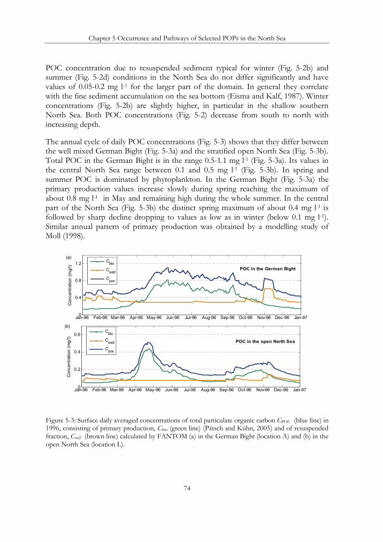
Chapter 5 Occurrence and Pathways of Selected POPs in the North Sea
74
POC concentration due to resuspended sediment typical for winter (Fig. 5-2b) and summer (Fig. 5-2d) conditions in the North Sea do not differ significantly and have values of 0.05-0.2 mg l-1 for the larger part of the domain. In general they correlate with the fine sediment accumulation on the sea bottom (Eisma and Kalf, 1987). Winter concentrations (Fig. 5-2b) are slightly higher, in particular in the shallow southern North Sea. Both POC concentrations (Fig. 5-2) decrease from south to north with increasing depth.
The annual cycle of daily POC concentrations (Fig. 5-3) shows that they differ between the well mixed German Bight (Fig. 5-3a) and the stratified open North Sea (Fig. 5-3b). Total POC in the German Bight is in the range 0.5-1.1 mg l-1 (Fig. 5-3a). Its values in the central North Sea range between 0.1 and 0.5 mg l-1 (Fig. 5-3b). In spring and summer POC is dominated by phytoplankton. In the German Bight (Fig. 5-3a) the primary production values increase slowly during spring reaching the maximum of about 0.8 mg l-1 in May and remaining high during the whole summer. In the central part of the North Sea (Fig. 5-3b) the distinct spring maximum of about 0.4 mg l-1 is followed by sharp decline dropping to values as low as in winter (below 0.1 mg l-1). Similar annual pattern of primary production was obtained by a modelling study of Moll (1998).
0
0.4
0.8
1.2
Jan-96 Feb-96 Mar-96 Apr-96 May-96 Jun-96 Jul-96 Aug-96 Sep-96 Oct-96 Nov-96 Dec-96 Jan-97
Con
cent
ratio
n (m
g/l)
0
0.2
0.4
0.6
Jan-96 Feb-96 Mar-96 Apr-96 May-96 Jun-96 Jul-96 Aug-96 Sep-96 Oct-96 Nov-96 Dec-96 Jan-97
Con
cent
ratio
n (m
g/l)
Cbio
Csed
Cpoc
Cbio
Csed
Cpoc
(a)
(b)
POC in the German Bight
POC in the open North Sea
Figure 5-3: Surface daily averaged concentrations of total particulate organic carbon CPOC (blue line) in 1996, consisting of primary production, Cbio (green line) (Pätsch and Kühn, 2005) and of resuspended fraction, Csed (brown line) calculated by FANTOM (a) in the German Bight (location A) and (b) in the open North Sea (location L).

Chapter 5 Occurrence and Pathways of Selected POPs in the North Sea
75
Resuspended sediment is an important contributor to the total POC content (Fig. 5.3). Resuspension of freshly deposited sediments occurs due to storm events which are more frequent in autumn and winter (Sündermann and Puls, 1990). This seasonality is more pronounced in the shallow German Bight (Fig. 5-3a) where disturbed sediment results in the POC concentration maximum of about 0.6 mg l-1 in November. Observations (van der Zee and Chou, 2005) also show that the contribution of resuspended POC to the total POC content is greater during winter. The central North Sea is deeper, thus the surface POC concentration (Fig. 5-3b) is less influenced by the resuspended portion which is also smaller.
The modelling results suggest that total POC concentration in the German Bight in winter is dominated by resuspended POC (75-85%). During summer the situation is opposite with up to 75% of POC resulting from primary production (Fig. 5-3a). In the central North Sea the winter POC content is equally distributed between the two constituents, whereas in summer the primary production makes up to 85% of the total content (Fig. 5-3b). These results are in a good agreement with other studies (Eisma and Kalf, 1987; Sündermann, 1994; Pohlmann and Puls, 1994; Moll, 1998; van der Zee and Chou, 2005).
5.1.2 Fraction of γ-HCH, α-HCH and PCB 153 on particulate organic carbon in sea water
Most of the POPs are moderately or very low water soluble (UNEP, 2003). Hydrophobic compounds – those not easily dissolved in water – are expected to be bound to POC and thus tend to disperse in the sediment rather than in the water phase. Measuring the concentration of non-water-soluble pollutants, e.g. PCB 153 in seawater is difficult because the concentrations often lie near to or below the detection limit for the substance.
Annual mean spatial distributions of γ-HCH, α-HCH and PCB 153 fractions bound to POC POCf expressed in % of the total sea water concentration (see Sect. 2.3.2) and averaged vertically for the whole modelling domain were calculated (Fig. 5-3a, b and c). Correspondent total POC concentration is shown on Fig. 5-3d. The location of the vertical section is shown on Fig. 5-1.
The amount of POP attached to organic matter is controlled by its lipophilicity often characterised by the octanol-water partition coefficient owK (see Sect. 2.3). Contaminants addressed in this study differ in their owK values (Table A-1) with PCB 153 being the most lipophilic with a owK value of 3 orders of magnitude higher than the one for γ-HCH and α-HCH. Consequently, calculated POCf for the two HCH isomer is about 0.15% in the whole North Sea (Fig. 5-4a and b) with the highest values
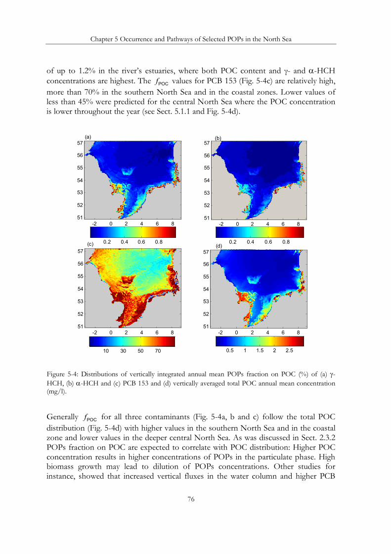
Chapter 5 Occurrence and Pathways of Selected POPs in the North Sea
76
of up to 1.2% in the river’s estuaries, where both POC content and γ- and α-HCH concentrations are highest. The POCf values for PCB 153 (Fig. 5-4c) are relatively high, more than 70% in the southern North Sea and in the coastal zones. Lower values of less than 45% were predicted for the central North Sea where the POC concentration is lower throughout the year (see Sect. 5.1.1 and Fig. 5-4d).
-2 0 2 4 6 851
52
53
54
55
56
57
-2 0 2 4 6 851
52
53
54
55
56
57
-2 0 2 4 6 851
52
53
54
55
56
57
-2 0 2 4 6 851
52
53
54
55
56
57
0.5 1 1.5 2 2.510 30 50 70
0.2 0.4 0.6 0.80.2 0.4 0.6 0.8
(a) (b)
(d)(c)
Figure 5-4: Distributions of vertically integrated annual mean POPs fraction on POC (%) of (a) γ-HCH, (b) α-HCH and (c) PCB 153 and (d) vertically averaged total POC annual mean concentration (mg/l).
Generally POCf for all three contaminants (Fig. 5-4a, b and c) follow the total POC distribution (Fig. 5-4d) with higher values in the southern North Sea and in the coastal zone and lower values in the deeper central North Sea. As was discussed in Sect. 2.3.2 POPs fraction on POC are expected to correlate with POC distribution: Higher POC concentration results in higher concentrations of POPs in the particulate phase. High biomass growth may lead to dilution of POPs concentrations. Other studies for instance, showed that increased vertical fluxes in the water column and higher PCB

Chapter 5 Occurrence and Pathways of Selected POPs in the North Sea
77
concentrations in phytoplankton due to eutrophication have been observed (Gunnarsson et al., 1995; Jeremiason et al., 1999; Dachs et al, 1999).
Another indication for the correlation between POC and POPs distribution is demonstrated by annual mean vertical distributions of γ-HCH, α-HCH and PCB 153 fractions bound to POC and correspondent POC concentration (Fig. 5-5a, b and c and Fig. 5-5d). POC concentrations (Fig. 5-5d) increase with depth due to higher content of resuspended sediment near the bottom and due to sinking of surface POC.
m
(a) γ-HCH51 52 53 54 55 56 57
0 5 10 15 20 25 30 35 40 45 50 60 70 80
0.1 0.2 0.3 0.4 0.5
m
(b) α-HCH51 52 53 54 55 56 57
0 5 10 15 20 25 30 35 40 45 50 60 70 80
0.1 0.2 0.3
m
(c) PCB 153(c) PCB 15351 52 53 54 55 56 57
0 5 10 15 20 25 30 35 40 45 50 60 70 80
m
(d) POC51 52 53 54 55 56 57
0 5 10 15 20 25 30 35 40 45 50 60 70 80
0.2 0.4 0.6 0.8 1 1.240 60 80
Figure 5-5: Vertical sections from south to north along 3oE (see Fig. 5-1) of annual mean POPs fraction on POC (%) of (a) γ-HCH, (b) α-HCH and (c) PCB 153 and (d) annual mean total POC concentration (mg/l).
Sinking organic carbon particles export contaminants to the lower water layers with their subsequent deposition at the bottom sediment.

Chapter 5 Occurrence and Pathways of Selected POPs in the North Sea
78
The annual cycle of daily averaged PCB 153 concentration in the particulate phase and its total sea water concentration in 1996 at locations A in the German Bight and L in the central North Sea are shown on Fig. 5-6a and b. Because both HCH isomers have very low particle-bound fraction values (Fig. 5-4 and Fig.5-5) they are not discussed here.
Uptake by biomass and subsequent sinking can deplete the dissolved concentrations of POPs in surface waters during periods of fast phytoplankton growth (Dachs et al., 1999; 2002; Schulz-Bull et al., 1995). The primary production in the North Sea generally shows a peak in spring followed by a decrease during the summer and a second peak in October-November caused by water column turnover (Moll, 1998). The dissolved concentration of PCB 153 in the North Sea is thus expected to high during winter with a decrease in spring followed by relatively low concentrations during summer and an increase during late autumn. This annual cycle is captured by the model (Fig. 5-6). Such annual cycle is supported by measurements conducted in the Kattegat Sea region (Sundqvist et al., 2004).
0
0.04
0.08
0.12
Jan-96 Feb-96 Mar-96 Apr-96 May-96 Jun-96 Jul-96 Aug-96 Sep-96 Oct-96 Nov-96 Dec-96 Jan-97
Con
cent
ratio
n (n
g/l)
0
0.004
0.008
0.012
Jan-96 Feb-96 Mar-96 Apr-96 May-96 Jun-96 Jul-96 Aug-96 Sep-96 Oct-96 Nov-96 Dec-96 Jan-97
Con
cent
ratio
n (n
g/l)
C PCB 153Cp PCB 153
C PCB 153Cp PCB 153
(a)
(b)
PCB 153 in the German Bight
PCB 153 in the open North Sea
Figure 5-6: PCB 153 total C and bound to particles pC concentrations at the sea surface: (a) in the German Bight (location A) and (b) in the open North Sea (location L).
Other studies suggest that eutrophic conditions lead to a depletion of water column concentrations of PCB 153 due to POC uptake and settling export (Dachs et al,. 1999). This hypothesis is supported by the model results showing that there is a link between
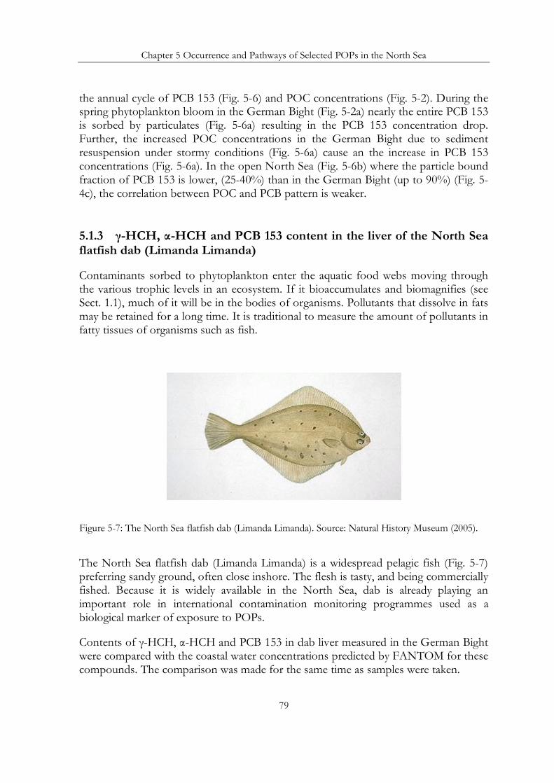
Chapter 5 Occurrence and Pathways of Selected POPs in the North Sea
79
the annual cycle of PCB 153 (Fig. 5-6) and POC concentrations (Fig. 5-2). During the spring phytoplankton bloom in the German Bight (Fig. 5-2a) nearly the entire PCB 153 is sorbed by particulates (Fig. 5-6a) resulting in the PCB 153 concentration drop. Further, the increased POC concentrations in the German Bight due to sediment resuspension under stormy conditions (Fig. 5-6a) cause an the increase in PCB 153 concentrations (Fig. 5-6a). In the open North Sea (Fig. 5-6b) where the particle bound fraction of PCB 153 is lower, (25-40%) than in the German Bight (up to 90%) (Fig. 5-4c), the correlation between POC and PCB pattern is weaker.
5.1.3 γ-HCH, α-HCH and PCB 153 content in the liver of the North Sea flatfish dab (Limanda Limanda)
Contaminants sorbed to phytoplankton enter the aquatic food webs moving through the various trophic levels in an ecosystem. If it bioaccumulates and biomagnifies (see Sect. 1.1), much of it will be in the bodies of organisms. Pollutants that dissolve in fats may be retained for a long time. It is traditional to measure the amount of pollutants in fatty tissues of organisms such as fish.
Figure 5-7: The North Sea flatfish dab (Limanda Limanda). Source: Natural History Museum (2005).
The North Sea flatfish dab (Limanda Limanda) is a widespread pelagic fish (Fig. 5-7) preferring sandy ground, often close inshore. The flesh is tasty, and being commercially fished. Because it is widely available in the North Sea, dab is already playing an important role in international contamination monitoring programmes used as a biological marker of exposure to POPs.
Contents of γ-HCH, α-HCH and PCB 153 in dab liver measured in the German Bight were compared with the coastal water concentrations predicted by FANTOM for these compounds. The comparison was made for the same time as samples were taken.

Chapter 5 Occurrence and Pathways of Selected POPs in the North Sea
80
1995 1996 1997 1998 1999 2000 20010
10
20
Conc
entra
tion
in d
ab (n
g/g
wet
wei
ght)
1995 1996 1997 1998 1999 2000 20010.5
1
1.5
1995 1996 1997 1998 1999 2000 20010
1
2
3
4
1995 1996 1997 1998 1999 2000 20010
0.1
0.2
0.3
0.4
1995 1996 1997 1998 1999 2000 20010
50
100
1995 1996 1997 1998 1999 2000 20010
0.05
0.1
Conc
entra
tion
in s
ea w
ater
(ng/
l)
(a) γ-HCH
(b) α-HCH
(c) PCB 153
Figure 5-8: Concentrations of γ-HCH, α-HCH and PCB 153 in flatfish dab liver (median values of individual measurements provided by the Institut für Fischereiökologie) measured in the German Bight (bars) and vertically integrated annual mean modelled by FANTOM sea water concentrations in the same location (dashed line).
Samples were taken in September each year according to the instructions of the respective guidelines for the marine monitoring programmes. The sampling period was chosen due to the fact that in late summer till early spring the fish are far away from spawning time (dab in the southern North Sea show considerably more migration during the spawning period). Furthermore dab is in relative good condition and so the natural shift is relatively low at that time. The dataset consists of data from individual

Chapter 5 Occurrence and Pathways of Selected POPs in the North Sea
81
fish samples where up to 25 fishes from the same area caught in the same or sometime two hauls were used.
The median values calculated from these data are presented in Fig. 5-8. The median reflects the results of one area and one day, but as the concentration in dab liver will not change as rapidly as in water and due to the selected sampling time the values will be adequate for a period of some weeks or even months (Haarich et al., 2005).
In the German Bight, within the investigation period from 1995 until 2001, only for α-HCH a steadily decreasing trend is observed (Fig. 5-8b). Lindane (Fig. 5-8a) shows low concentrations in the beginning, followed by an increase with a turning point in 1996. The highest concentrations both in dab and in sea water were in 1997. After 1998 lindane concentrations were decreasing continuously in both dab and sea water. High γ-HCH concentrations in the German Bight in 1995 can be explained by high runoff from the Elbe river in autumn 1995, where a correlation between the wet weight-based concentrations and suspended matter concentrations could be confirmed (v. Westernhagen et al., 2000). For PCB 153 (Fig. 5-8c) dab and sea water concentrations in the end of the investigated time period were higher than in the beginning.
Modelled sea water concentrations for all three contaminants follow the pattern detected in dab (Fig. 5-8). As demonstrated by Fig. 5-8 due to persistence and bioaccumulation even very low contaminant concentrations in sea water can lead to much higher concentrations in fish, marine mammals and fish-eating birds. In spite of total reduced inputs of the investigated contaminants, their concentrations in dab have not decreased continuously in the German Bight and also in other regions of the North Sea (Lang and Wosniok, 2003). According to OSPAR assessment (OSPAR, 2000) concentrations of organochlorines in fish from the North Sea are still 3 to 10 times higher than in catches from the Northern Atlantic.
5.2 Spatial and temporal distribution of γ-HCH, α-HCH and PCB 153 in sea water
5.2.1 γ-HCH horizontal and vertical distributions
Measurements in the North Sea’s uppermost layer of 5 m thickness compiled during summer 1995 and interpolated on the modelling domain of FANTOM (Fig. 3-5) show clear gradients of γ-HCH with the highest concentrations in the southern regions of the North Sea, in the estuaries of rivers and in the English Channel. The highest concentration of 8 ng l-1 was found close to the mouth of the River Elbe.

Chapter 5 Occurrence and Pathways of Selected POPs in the North Sea
82
Annual mean γ-HCH concentrations averaged vertically for the whole modelling domain in the years 1996–2001 were calculated (Fig. 5-12). These results show positive gradients of concentration towards the coasts; a similar pattern was found in the initial distribution (Fig. 3-5). During the 1995–1997 total concentration of γ-HCH in the continental coastal water was above 1 ng l-1 with a concentration of more than 25 ng l-1 in the River Elbe estuary. As with the γ-HCH concentration at the selected locations (Fig. 4-2 and Fig. 4-3), concentrations in the whole modelling domain decreased. This effect is more pronounced in the southern regions of the North Sea where initial concentrations had been highest.
Vertical distribution of sea temperature and salinity in January and August 1997 and correspondent γ-HCH distribution from south to north along the 3°E are plotted in Fig. 5-9.
m
33.6
33.6
33.7
33.7
33.8
33.8
33.8
3 3.9
3 3.9
3434
.134
.23 4
.234
.334
.33 4
.434
.434
.534
.534
.634
.6
34.7
51 52 53 54 55 56 57 0
5
10
15
20
25
30
35
40
45
50
60
70
80
2 3 4 5 6
m
33. 8
33.8
3 3.8
33.8 33
. 9
33. 9
34
34 34.134
.1
34. 2
34.334 .4
34. 5
3 4.5
34. 6
34 .634.7
51 52 53 54 55 56 57 0
5
10
15
20
25
30
35
40
45
50
60
70
80
4 6 8 10 12 14 16
m51 52 53 54 55 56 57
0
5
10
15
20
25
30
35
40
45
50
60
70
80
0.2 0.4 0.6 0.8 1 1.2
m
51 52 53 54 55 56 57 0
5
10
15
20
25
30
35
40
45
50
60
70
80
0.2 0.4 0.6 0.8 1 1.2
(a) (b)
(c) (d)
Figure 5-9. Vertical sections from south to north along 3°E of sea temperature (colours, °C) and salinity (lines) in January (a) and August (c) 1997 calculated by HAMSOM and corresponding γ-HCH total concentrations (ng/l) (b and d) calculated by FANTOM.
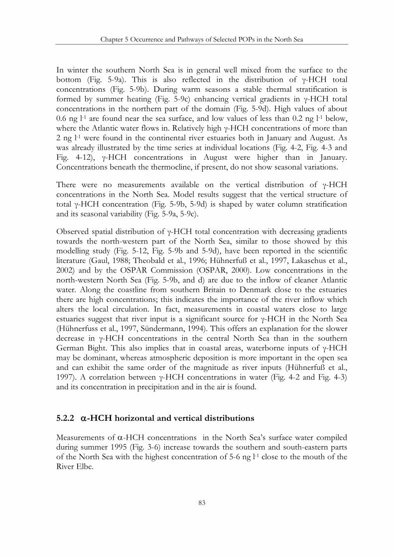
Chapter 5 Occurrence and Pathways of Selected POPs in the North Sea
83
In winter the southern North Sea is in general well mixed from the surface to the bottom (Fig. 5-9a). This is also reflected in the distribution of γ-HCH total concentrations (Fig. 5-9b). During warm seasons a stable thermal stratification is formed by summer heating (Fig. 5-9c) enhancing vertical gradients in γ-HCH total concentrations in the northern part of the domain (Fig. 5-9d). High values of about 0.6 ng l-1 are found near the sea surface, and low values of less than 0.2 ng l-1 below, where the Atlantic water flows in. Relatively high γ-HCH concentrations of more than 2 ng l-1 were found in the continental river estuaries both in January and August. As was already illustrated by the time series at individual locations (Fig. 4-2, Fig. 4-3 and Fig. 4-12), γ-HCH concentrations in August were higher than in January. Concentrations beneath the thermocline, if present, do not show seasonal variations.
There were no measurements available on the vertical distribution of γ-HCH concentrations in the North Sea. Model results suggest that the vertical structure of total γ-HCH concentration (Fig. 5-9b, 5-9d) is shaped by water column stratification and its seasonal variability (Fig. 5-9a, 5-9c).
Observed spatial distribution of γ-HCH total concentration with decreasing gradients towards the north-western part of the North Sea, similar to those showed by this modelling study (Fig. 5-12, Fig. 5-9b and 5-9d), have been reported in the scientific literature (Gaul, 1988; Theobald et al., 1996; Hühnerfuß et al., 1997, Lakaschus et al., 2002) and by the OSPAR Commission (OSPAR, 2000). Low concentrations in the north-western North Sea (Fig. 5-9b, and d) are due to the inflow of cleaner Atlantic water. Along the coastline from southern Britain to Denmark close to the estuaries there are high concentrations; this indicates the importance of the river inflow which alters the local circulation. In fact, measurements in coastal waters close to large estuaries suggest that river input is a significant source for γ-HCH in the North Sea (Hühnerfuss et al., 1997, Sündermann, 1994). This offers an explanation for the slower decrease in γ-HCH concentrations in the central North Sea than in the southern German Bight. This also implies that in coastal areas, waterborne inputs of γ-HCH may be dominant, whereas atmospheric deposition is more important in the open sea and can exhibit the same order of the magnitude as river inputs (Hühnerfuß et al., 1997). A correlation between γ-HCH concentrations in water (Fig. 4-2 and Fig. 4-3) and its concentration in precipitation and in the air is found.
5.2.2 α-HCH horizontal and vertical distributions
Measurements of α-HCH concentrations in the North Sea’s surface water compiled during summer 1995 (Fig. 3-6) increase towards the southern and south-eastern parts of the North Sea with the highest concentration of 5-6 ng l-1 close to the mouth of the River Elbe.

Chapter 5 Occurrence and Pathways of Selected POPs in the North Sea
84
Annual mean α-HCH concentrations averaged vertically for the whole modelling domain in the years 1996–2001 were calculated (Fig. 5-13). These results show positive gradients of concentration towards the coasts; a similar pattern was found in the initial distribution (Fig. 3-6). During 1995–1998 the concentration of α-HCH in the continental coastal water was about 0.3 ng l-1 with a concentration of more than 5 ng l-1 in the River Elbe estuary. Concentrations in the central and north-western parts of the North Sea were about 0.2 ng l-1. Concentrations of α-HCH decreased further during 1999-2001 remaining below 0.2 ng l-1 in nearly the entire North Sea, except for the river estuaries, indicating that rivers still contribute significantly to the α-HCH burden, in particular in the coastal zones. As was already demonstrated by α-HCH concentrations at selected locations (Fig. 4-6 and 4-7), concentrations in the whole modelling domain decreased over the simulation period.
m
51 52 53 54 55 56 57 0
5
10
15
20
25
30
35
40
45
50
60
70
80
m
51 52 53 54 55 56 57 0
5
10
15
20
25
30
35
40
45
50
60
70
80
0.05
0.1
0.15
0.2
0.25
0.3
(a) (b)
Figure 5-10: Vertical sections from south to north along 30E of α-HCH total concentrations in January (a) and August (b) 1997 calculated by FANTOM.
Although α- and γ-HCHs possess similar physical-chemical properties (see Sect. 3.3) their environmental behaviour is different due to various inputs throughout the last decades. Therefore the two isomers have noticeably different distributions in the North Sea. First of all α-HCH sea water concentrations had been decreasing steadily throughout the simulation period, whereas γ-HCH concentrations experienced an increase in 1997-1998. Secondly, unlike γ-HCH temporal distribution, for which the decrease was more pronounced in the southern regions of the North Sea where initial concentrations had been highest, α-HCH decreased more or less homogeneously. This result from the use of pure lindane (γ-HCH) in western Europe (SRU, 2004). Thus, α-HCH can come only from degradation of γ-HCH or atmospheric transport.
Chapter 5 Occurrence and Pathways of Selected POPs in the North Sea
85
Vertical distribution of α-HCH concentration in January and August 1997 from south to north along 3°E (Fig. 5-1) are plotted in Fig. 5-10. Winter concentrations of α-HCH are well mixed along the section, as well as the water masses (Fig. 5-9a). The model predicts vertical gradients in α-HCH concentrations in the northern deeper part of the North Sea (Fig. 5-10b). Similar to γ-HCH vertical distributions, model results for α-HCH suggest that the vertical concentration pattern (Fig. 5-10) is shaped by water column stratification and its seasonal variability (Fig. 5-9a and c).
5.2.3 PCB 153 horizontal and vertical distributions
Annual mean PCB 153 concentrations averaged vertically for the whole modelling domain in the years 1996–2001 were calculated (Fig. 5-14). Generally, concentrations decline moving offshore. Although concentrations in the continental estuaries and in the Thames estuary off the East Anglian coast are higher than in the English Channel and in the central North Sea. Measurements of PCB 153 concentrations in the North Sea’s surface water compiled during summer 1995 and interpolated on the modelling domain of FANTOM (Fig. 3-7) show positive gradients towards the east, with the highest concentrations in the eastern and south-eastern parts of the North Sea. The highest concentration of 0.16 ng l-1 was found close to the mouth of the River Elbe.
m
51 52 53 54 55 56 57 0
5
10
15
20
25
30
35
40
45
50
60
70
80
m
51 52 53 54 55 56 57 0
5
10
15
20
25
30
35
40
45
50
60
70
80
1
2
3
4
5
6
7
8
x 10-3
(a) (b)
Figure 5-12: Vertical sections from south to north along 3°E of PCB 153 total concentrations (ng/l) in January (a) and August (b) 1997 calculated by FANTOM.

Chapter 5 Occurrence and Pathways of Selected POPs in the North Sea
86
This pattern remains throughout the entire simulation period. Concentrations of PCB 153 in 1995-2000 (Fig. 5-14a, b, c and d) do not show any pronounced trend with the values between 0.025-0.05 ng l-1 in the southern North Sea and less than 0.01 ng l-1 in the central North Sea. In 2000 (Fig. 5-14e) and further on the modelled concentrations show an increase with values more than 0.035 ng l-1 nearly in the entire North Sea in 2001 (Fig. 5-14f). As was shown before (Sect. 4.4) this increase was detected also in the measured sea water, riverine and atmospheric concentrations.
Vertical distribution of PCB 153 concentration in January and August 1997 from south to north along the 3°E is plotted in Fig. 5-11. The vertical profile structure for PCB 153 calculated by FANTOM looks different from the one of the two HCH isomers (Fig. 5-9 and Fig. 5-10). This is especially evident for the winter distribution of PCB 153 (Fig. 5-11a). A clearly defined stratification of PCB 153 January concentration (Fig. 5-11a) in well mixed water mass (Fig. 5-9a) is predicted by the model. As was illustrated in Sect. 5.1 PCB 153 is mostly bound to particulate matter in sea water, whereas α- and γ-HCH are prevailingly dissolved. The model results suggest that distribution of the particle bound fraction of PCB 153 follows the POC distribution (Fig. 5-4 and Fig. 5-5). Because of sinking and resuspension of newly deposited sediments, higher concentrations of particulate matter are accumulated near the bottom. This phenomenon is reflected in the vertical distribution of PCB 153 with prevailing share of particle-bound concentration (Fig. 5-11a).
The modelled vertical distribution of PCB 153 in August (Fig. 5-11b) does not show the same structure as in January suggesting that they were shaped by non-intermediate storm events typical for winter periods in the North Sea. Indeed, the summer PCB 153 concentration pattern (Fig. 5-11b) is similar to the one of α- and γ-HCHs (Fig. 5-9d and Fig. 5-10b) influenced by the thermal stratification occurring in summer. The model outcomes are also supported by the measurements results in the German Bight reported by Hühnerfuss et al. (1997).
Due to high persistence and volatility PCB 153 undergo long range transport in the atmosphere. One open question is whether the PCB 153 sea water concentrations are still largely controlled by primary discharges or by re-emission from the sediments a major repository of PCBs in aquatic environment. Recent studies are in favour of the primary emissions. Other contaminated water bodies such as the Great Lakes of North America have been reported to currently be net sources of PCBs to the atmosphere as a result of the release of PCBs which have accumulated in the sediments (Jeremiason et al., 1994). The mass balance studies performed by Wania et al. (2001) and Axelman and Broman (2001) indicate that the Baltic Sea is a net sink of PCBs. The phenomenon illustrated by Fig. 5-11a shows the significance of the sediment contribution to the sea water PCB 153 burden.

Chapter 5 Occurrence and Pathways of Selected POPs in the North Sea
87
1996
(a)
-2 0 2 4 6 851
52
53
54
55
56
57
1997
(b)
-2 0 2 4 6 851
52
53
54
55
56
57
1998
(c)
-2 0 2 4 6 851
52
53
54
55
56
57
1999
(d)
-2 0 2 4 6 851
52
53
54
55
56
57
2000
(e)
-2 0 2 4 6 851
52
53
54
55
56
57
2001
(f)
-2 0 2 4 6 851
52
53
54
55
56
57
0.5 1 1.5 2
Figure 5-12. Vertically integrated annual mean concentrations of γ-HCH (ng/l) in the North Sea calculated by FANTOM.

Chapter 5 Occurrence and Pathways of Selected POPs in the North Sea
88
1996
(a)
-2 0 2 4 6 851
52
53
54
55
56
57
1997
(b)
-2 0 2 4 6 851
52
53
54
55
56
57
1998
(c)
-2 0 2 4 6 851
52
53
54
55
56
57
1999
(d)
-2 0 2 4 6 851
52
53
54
55
56
57
2000
(e)
-2 0 2 4 6 851
52
53
54
55
56
57
2001
(f)
-2 0 2 4 6 851
52
53
54
55
56
57
0.05 0.1 0.15 0.2 0.25 0.3 0.35 0.4 0.45
Figure 5-13. Vertically integrated annual mean concentrations of α-HCH (ng/l) in the North Sea calculated by FANTOM.

Chapter 5 Occurrence and Pathways of Selected POPs in the North Sea
89
1996
(a)
1996
(a)
1996
(a)
-2 0 2 4 6 851
52
53
54
55
56
57
1997
(b)
1997
(b)
1997
(b)
-2 0 2 4 6 851
52
53
54
55
56
57
1998
(c)
1998
(c)
1998
(c)
-2 0 2 4 6 851
52
53
54
55
56
57
1999
(d)
1999
(d)
1999
(d)
-2 0 2 4 6 851
52
53
54
55
56
57
2000
(e)
2000
(e)
2000
(e)
-2 0 2 4 6 851
52
53
54
55
56
57
2001
(f)
2001
(f)
2001
(f)
-2 0 2 4 6 851
52
53
54
55
56
57
0.005 0.01 0.015 0.02 0.025 0.03 0.035 0.04 0.045
Figure 5-14. Vertically averaged annual mean concentrations of PCB 153 (ng/l) in the North Sea calculated by FANTOM.

Chapter 5 Occurrence and Pathways of Selected POPs in the North Sea
90
5.3 α-HCH to γ-HCH ratio in sea water Alpha- and gamma-HCH are the most prevalent isomers in soil, water, and air samples. The ratio of alpha- to gamma- isomers can be used to track global transport of HCHs. Ratios of α/ γ-HCH together with concentrations of each isomer are useful source indicators. The α/γ-HCH ratio is an indicator of current technical HCH application. It can also indicate that present concentrations are being influenced by past use of technical HCH. When technical HCH mixture is the HCH source, α/β and α/γ ratios lie between 5 and 11 and 3 and 7, respectively (Jantunen and Bidleman 1996, Chernyak et al. 1996, Hargrave et al. 1988).
-2 0 2 4 6 851
52
53
54
55
56
57
0.1 0.2 0.3
-2 0 2 4 6 851
52
53
54
55
56
57(a) (b)
January July
Figure 5-15. Monthly mean α/γ-HCH ratio (based on surface concentrations) in sea water in January (a) and July (b) 1997 calculated by FANTOM.
Furthermore, the α/γ-HCH ratio can be used to estimate the age of the air and water masses (Oehme 1991). Air or water masses are considered as being old (or POPs are transported over long distance) when the α/γ-HCH ratio is greater than 3 (Lane et al. 1992; Jantunen and Bidleman, 1997) and as being young (or indicating fresh application of HCH) when the α/γ-HCH ratio is less than 1 (Hoff et al. 1992; Lakaschus et al. 2001). The ratio is strongly influenced by variable partitioning and persistence of the two isomers.
Spatial distribution of α/γ-HCH ratio typical for winter and summer were calculated from the surface α- and γ-HCH concentrations (Fig. 5-15). As was shown before (see Sect. 5.2.1 and 5.2.2), the vertical distributions of α and γ-HCH sea water concentrations (Fig. 5-9 and Fig. 5-10) were very similar in winter and summer, mainly

Chapter 5 Occurrence and Pathways of Selected POPs in the North Sea
91
shaped by the water mass stratification. Therefore, it is adequate to use surface sea water concentrations for further analysis. A lindane source will show α/γ-HCH ratio near or less than unity. The modelled α/γ-HCH ratio less than 1 in the entire North Sea could be explained by the ban of technical HCH more than two decades ago and by the geographic remoteness of the North Sea from the regions where technical HCH is applied (e.g. India, Philippines). High α/γ-HCH ratios are observed in the Sea of Japan and Okhotsk, as well as in the Chukchi and East and South China Seas (Olsson, 2002). The γ-HCH arriving to the North Sea comes not only from around the site but also via long-range transport. The α/γ-HCH ratios for the central parts of the North Sea are low (<0.5), so we can consider local emissions predominant and the water masses young. Winter values (Fig. 5-15a) of the α/γ-HCH ratio are 0.3-0.5 higher than the summer ones (Fig. 5-15b) which are 0.1-0.2 caused by higher inputs of γ-HCH from rivers and atmosphere during summer. The higher levels found in winter are influenced by the low temperatures, and the presence of a thermocline, which minimises mixing and dilution.
The ratios between α- and γ-HCH isomers can be used to explore time trends, because the relative concentrations are less affected by methodological differences. Temporal distributions of α/γ-HCH at different locations of the North Sea based on the daily averaged sea surface concentrations are calculated and compared with the correspondent ratios derived from measurements (Fig. 5-16). There was no pronounced trend in α/γ-HCH ratio predicted for the simulation period. Besides the annual signal, the values in the end of the simulation period are within a factor of 2 with regard to the starting values in all four locations (Fig. 5-16). In general, the α/γ-HCH ratio resulted from FANTOM calculations are in good agreement with observations. The underestimated values at location N near the English Channel are probably due to the overestimated lindane concentrations in this region as was discussed in Sect. 4.2. Other studies based on observations (Iwata et al., 1993; Lakaschus et al., 2002) showed that the α/γ-HCH ratio is observed to increase pole-ward, only to decrease on the Atlantic side as a result of present usage of lindane in this region.

Chapter 5 Occurrence and Pathways of Selected POPs in the North Sea
92
0
0.4
0.8
Jan-96 Jul-96 Jan-97 Jul-97 Jan-98 Jul-98 Jan-99 Jul-99 Jan-00 Jul-00 Jan-01 Jul-01 Jun-95 Jan-02
0
0.4
0.8
Jan-96 Jul-96 Jan-97 Jul-97 Jan-98 Jul-98 Jan-99 Jul-99 Jan-00 Jul-00 Jan-01 Jul-01 Jun-95 Jan-02
0
0.4
0.8
Jan-96 Jul-96 Jan-97 Jul-97 Jan-98 Jul-98 Jan-99 Jul-99 Jan-00 Jul-00 Jan-01 Jul-01 Jun-95 Jan-02
0
0.4
0.8
Jan-96 Jul-96 Jan-97 Jul-97 Jan-98 Jul-98 Jan-99 Jul-99 Jan-00 Jul-00 Jan-01 Jul-01 Jun-95 Jan-02
A
J
L
N
(a)
(b)
(c)
(d)
Figure 5-16. α/γ-HCH concentration ratio in sea water at the locations A, J, L, N. Solid lines are model results derived from the main runs for α-HCH and γ-HCH; dashed lines are derived from observations.

Chapter 6 Contribution of Individual Processes to the Cycling of Selected POPs in the North Sea
93
Chapter 6
Contribution of Individual Processes to the Cycling of Selected POPs in the North Sea
A deeper insight on the pathways of contaminants in the environment can be obtained through their mass budgets in the respective compartments. Such budget calculations for the North Sea based on the measurement results were already performed for cadmium, several organic contaminants (namely HCHs, PCBs and triazines), suspended matter and nutrients. These calculations resulted from the PRISMA11 and ZISCH12 experiments (Sündermann and Radach, 1997). The present study is the first attempt to estimate mass budgets of the three POPs based on a model calculations. Mass budgets were calculated for individual years within the simulation period for the entire modelling domain and for the inner German Bight (Sect. 6.1). The residence times of the three POPs were calculated in order to understand the export and import relationships of the driving processes in the fate of POPs (Sect. 6.2). The contribution of the key processes to the burden of these POPs in the North Sea and in the German Bight are presented based on
(a) Modelling scenarios when one key process was switched off for the entire simulation period (Sect. 6.3.1).
(b) Dependencies of some processes on the environmental parameters, i.e. wind speed and sea surface and air temperatures (Sect. 6.3.2).
11 Prozesse im Schadstoffkreislauf Meer-atmosphäre (PRISMA). 12 Zirkulation und Schadstoffkreislauf in der Nordsee (ZISCH).
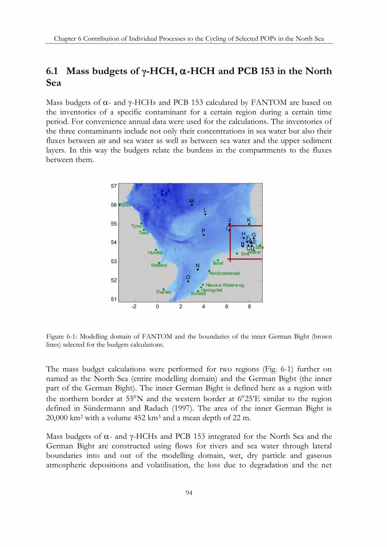
Chapter 6 Contribution of Individual Processes to the Cycling of Selected POPs in the North Sea
94
6.1 Mass budgets of γ-HCH, α-HCH and PCB 153 in the North Sea
Mass budgets of α- and γ-HCHs and PCB 153 calculated by FANTOM are based on the inventories of a specific contaminant for a certain region during a certain time period. For convenience annual data were used for the calculations. The inventories of the three contaminants include not only their concentrations in sea water but also their fluxes between air and sea water as well as between sea water and the upper sediment layers. In this way the budgets relate the burdens in the compartments to the fluxes between them.
Figure 6-1: Modelling domain of FANTOM and the boundaries of the inner German Bight (brown lines) selected for the budgets calculations.
The mass budget calculations were performed for two regions (Fig. 6-1) further on named as the North Sea (entire modelling domain) and the German Bight (the inner part of the German Bight). The inner German Bight is defined here as a region with the northern border at 55°N and the western border at 6°25’E similar to the region defined in Sündermann and Radach (1997). The area of the inner German Bight is 20,000 km2 with a volume 452 km3 and a mean depth of 22 m.
Mass budgets of α- and γ-HCHs and PCB 153 integrated for the North Sea and the German Bight are constructed using flows for rivers and sea water through lateral boundaries into and out of the modelling domain, wet, dry particle and gaseous atmospheric depositions and volatilisation, the loss due to degradation and the net
AB
C
L
M
H GI
N
K
O
P
J
DE
F
HaringvlietScheldt
Nieuw e Waterw eg
Nordzeekanaal
Ijssel
EmsWeserElbe
Thames
Humber
Tyne
Forth
Welland
Tees
-2 0 2 4 6 851
52
53
54
55
56
57

Chapter 6 Contribution of Individual Processes to the Cycling of Selected POPs in the North Sea
95
transfer to the bottom sediments. The mass balance equation of these processes described in Chapter 2 can be written as:
6-1
The survey of the model results on the mass budgets calculations for γ-, α-HCHs and PCB 153 in the North Sea and the inner German Bight are summarised in Tables 6-1, 6-2 and Table 6-3 and plotted in Fig. 6-2 and Fig. 6-3.
Table 6-1: Cumulative contributions of different processes calculated by FANTOM in the γ-HCH yearly mass budgets in kg a-1.
γ-HCH Processes contribution North Sea German Bight
[kg/a] 1996 1997 1998 1999 2000 2001 1996 1997 1998 1999 2000 2001
Wet deposition 5470.25 7074.4 4838 3480.65 3019.48 1673.42 350 453 310 223 193 107
Dry particle deposition 0.05218 0.04302 0.04389 0.02281 0.01788 0.01118 0.0033 0.0027 0.0028 0.0015 0.0011 0.0007
Dry gaseous deposition 8849.8 8562.3 8902.1 4854.7 3654.3 2339.1 761.07 780.03 811.11 439.28 338.44 210.32
Volatilisation 3415.3 3865 3498.9 2427.4 2059.3 1587.6 605.25 885.33 861.8 514.19 449.65 326.11
Degradation 2.49 3.41 2.69 1.93 1.7 1.26 0.16 0.22 0.17 0.12 0.11 0.08
Sinking 1964.9 2239.2 2064 1478.7 1308.8 983.19 63.8 72.7 67 48 42.5 31.91
Resuspension 213.92 241.66 207.91 138.2 116.67 98.123 6.94 7.84 6.75 4.49 3.79 3.19
River inflow 430.56 646.72 554.15 398.86 317.07 243.14 169.01 356.03 260.55 103.32 135.71 67.295
Lateral boundaries inflow 8273.5 7803.6 8410.6 8174 8399 7902.8 4339.6 5345.6 5427.8 3531.64 3044.9 2337.46
Lateral boundaries outflow 8415.43 8650.46 9716.3 9453.93 10044.11 8226.23 4474 5632.3 6096.4 3862.04 3274.35 2542.79
Total 3028.7 3291.7 2830.3 1931.3 1689.7 1388 313.221 422.390 415.019 237.515 213.592 178.727
∫∫∫
∫∫∫∫
∫∫∫
+−−
−+++
+−=−
ttt
tttt
ttt
t
dtResuspendtSinkingdtDegrad
dtVolatildtGasDepdtPartDepdtWetDep
dtRiversdtOutflowdtInflowMM
000
0000
0000
][][][
][][][][
][][][

Chapter 6 Contribution of Individual Processes to the Cycling of Selected POPs in the North Sea
96
Table 6-2: Cumulative contributions of different processes calculated by FANTOM in the α-HCH yearly mass budgets in kg a-1.
α-HCH Processes contribution North Sea German Bight
[kg/a] 1996 1997 1998 1999 2000 2001 1996 1997 1998 1999 2000 2001
Wet deposition 811.55 346.17 350.58 473.5 249.05 218.75 51.96 22.16 22.45 30.32 15.95 14.01
Dry particle deposition 0.0138 0.0101 0.0075 0.0048 0.0036 0.0034 0.00089 0.00065 0.00048 0.00030 0.00023 0.00021
Dry gaseous deposition 8978.3 7082.1 5893.8 3780.7 2949.9 2564.8 774.76 641.18 530.24 338.27 277.62 235.02
Volatilisation 4294.3 3745.9 3112.1 2242.1 1210.9 982.79 667.44 681.18 840.99 420.21 277.59 183.81
Degradation 2.7364 2.3641 1.8021 1.2815 1.2071 1.0405 0.18 0.15 0.12 0.08 0.08 0.07
Sinking 966.87 852.36 744.63 501.76 530.57 385.5 31.39 27.67 24.17 16.29 17.22 12.51
Resuspension 50.013 44.801 35.107 24.432 24.547 21.398 1.62 1.45 1.14 0.79 0.80 0.69
River inflow 258.5 265.7 558.78 257.41 308.22 201.26 151.61 183.49 468.76 102.2 155.02 85.814
Lateral boundaries
inflow 2808.7 2850.6 3161.9 3009.3 3017.5 3017.3 1395.53 1314.41 1107.21 780.96 782.72 557.1
Lateral boundaries
outflow 3884.5 3765.9 3922.1 3746.1 4100.6 3352.6 1460.32 1378.19 1246.69 870.17 888.61 619.82
Total 1173 1013.4 772.48 549.33 517.42 446.02 141.094 143.318 151.109 59.788 50.673 38.897
Table 6-3: Cumulative contributions of different processes calculated by FANTOM in the PCB 153 yearly mass budgets in kg a-1.
PCB 153 Processes contribution North Sea German Bight
[kg/a] 1996 1997 1998 1999 2000 2001 1996 1997 1998 1999 2000 2001
Wet deposition 266.58 301.1 350.76 326.7 358.16 457.81 4.233 9.521 5.460 5.837 7.212 16.668
Dry particle deposition
9.13E-06
5.62E-06
6.00E-06
5.34E-06
6.17E-06
5.25E-06
5.84E-07
3.60E-07
3.84E-07
3.42E-07
3.95E-07
3.36E-07
Dry gaseous deposition 106.25 74.15 95.06 82.47 99.29 72.71 8.9499 6.2955 7.4858 6.4532 7.9016 5.5588
Volatilisation 66.11 148.71 85.27 91.17 112.64 260.33 55.562 46.828 128.43 109.26 111.38 117.81
Degradation 2.08 2.83 2.29 2.2 2.52 2.91 0.133 0.181 0.147 0.141 0.161 0.186
Sinking 486.89 626.65 546.81 522.39 606.11 659.51 15.81 20.34 17.75 16.96 19.68 21.41
Resuspension 195.45 420.85 406.66 280.58 374.17 596.38 6.34 13.66 13.20 9.11 12.15 19.36
River inflow 37.45 28.85 11.23 95.32 91.78 86.72 32.889 23.82 105.37 87.968 84.899 78.653
Lateral boundaries inflow 71.9 73.3 85.8 82.4 79.8 79.5 30.362 80.801 117.177 57.081 111.729 216.44
Lateral boundaries outflow 83.7 80.5 85.3 82.3 88.6 73.1 45.357 112.47 164.464 112.126 175.816 260.61
Total 1333.95 1716.85 1498.12 1431.23 1660.6 1806.9 278.029 267.010 548.533 478.654 516.411 464.976

Chapter 6 Contribution of Individual Processes to the Cycling of Selected POPs in the North Sea
97
1,00E+00
1,00E+01
1,00E+02
1,00E+03
1,00E+04
1996 1997 1998 1999 2000 2001
kg
dry deposition
wet deposition
volatill isation
s inking
resuspension
rivers inflow
degradation
inflow AO
outflow AO
inflow EC
outflow EC
1,00E-02
1,00E-01
1,00E+00
1,00E+01
1,00E+02
1,00E+03
1,00E+04
1996 1997 1998 1999 2000 2001
kg
1,00E-04
1,00E-03
1,00E-02
1,00E-01
1,00E+00
1,00E+01
1,00E+02
1,00E+03
1996 1997 1998 1999 2000 2001
kg
(c) PCB 153
(b) α-HCH
(a) γ-HCH North Sea
Figure 6-2: Cumulative masses (kg) calculated by FANTOM (for entire modelling domain, for each year) for γ-HCH (a), α-HCH (b) and PCB 153 (c) contributed by different processes acting in sea water as sources, i.e.: dry and wet atmospheric deposition, resuspension from the sea bottom, rivers inflow, inflow from the Atlantic Ocean (through the northern boundary) and from the English Channel (southern boundary); or sinks, i.e.: volatilisation, sinking to the sea bottom, degradation, outflow through the northern and southern boundaries.
Because the processes presented on Fig. 6-2 and 6-3 differ in their scales (i.e. contribution of dry gaseous deposition into γ-HCH burden is almost 4 orders of magnitude larger than degradation), the results are presented on a logarithmic scale with values given in Tables 6-1, 6-2 and 6-3.

Chapter 6 Contribution of Individual Processes to the Cycling of Selected POPs in the North Sea
98
(a) γ-HCH German Bight
1,00E-02
1,00E-01
1,00E+00
1,00E+01
1,00E+02
1,00E+03
1,00E+04
1996 1997 1998 1999 2000 2001
kg
dry deposition
wet deposition
volatill isation
s inking
resuspension
rivers inflow
degradation
inflow North
outflow North
inflow West
outflow West
1,00E-02
1,00E-01
1,00E+00
1,00E+01
1,00E+02
1,00E+03
1,00E+04
1996 1997 1998 1999 2000 2001
kg
(b) α-HCH
1,00E-01
1,00E+00
1,00E+01
1,00E+02
1,00E+03
1996 1997 1998 1999 2000 2001
kg
(c) PCB 153
Figure 6-3: Cumulative masses (kg) calculated by FANTOM (for the inner German Bight, for each year) for γ-HCH (a), α-HCH (b) and PCB 153 (c) contributed by different processes acting in sea water as sources, i.e.: dry and wet atmospheric deposition, resuspension from the sea bottom, rivers inflow, inflow through the western and the northern boundaries or sinks, i.e.: volatilisation, sinking to the sea bottom, degradation and outflow through the northern and western boundaries.
The question which is addressed in this section is whether the contribution of these processes to the contaminant burden is similar for the entire North Sea and for the German Bight. The following sections present analysis of the obtained annual budget calculations separately for the three substances.

Chapter 6 Contribution of Individual Processes to the Cycling of Selected POPs in the North Sea
99
6.1.1 Mass budget analysis for γ-HCH
In the case of γ-HCH, the largest input for the North Sea (Fig. 6-2a) for all six years occurs through gaseous atmospheric deposition and the lateral transport with ocean currents. The total atmospheric deposition (wet, dry gaseous and particle deposition) is much higher than the total flow through water pathways, i.e. in- and outflows through the lateral boundaries and river inflow. Although the volatilisation flux has the same order of magnitude as the gas depositional one, the net flux is positive for the North Sea as a whole (Fig. 6-2a). The model results also suggest that deposition of particles is negligibly low compared to other depositional processes. However, compared to the whole North Sea (Fig. 6-2a), the atmospheric input of lindane becomes less important in the scale of the inner German Bight (Fig. 6-3a).
The model results suggest that the river inflow does is not the most dominant source with the values of more than one order of magnitude below those for the flux from the atmosphere (Table 6-1). The inflow through the southern oceanic boundary was always greater than the outflow. This results support the conclusions made in the previous chapters that the English Channel contributed to the North Sea burden of lindane throughout the simulation period (see Chapter 4). Large values of outflow through the northern oceanic boundary (Fig. 6-2a) indicate the North Sea is influenced mainly by local discharges of γ-HCH.
In the German Bight the distribution of γ-HCH burdens between the processes differs from the one in the entire North Sea (Fig. 6-3a and Table 6-1). First of all this is seen in the air-sea gaseous flux direction. The model results suggest that the German Bight volatilised lindane throughout the entire simulation period (Fig. 6-3a). Spatial distributions of lindane in the German Bight (Chapter 4 and 5) showed increasing gradients towards the coast. High concentrations there are due to the proximity to the River Elbe and also due to the cyclonic circulation pattern in the North Sea. Indeed, the relative importance of the inflow from the rivers (the rivers Elbe, Weser and Ems) in the German Bight is higher than for the North Sea as a whole. The contribution from river inflow was up to 11% of the total input in the German Bight and less than 2% in the whole North Sea (Table 6-1) varying between 0.65 t a-1 and 0.24 t a-1 for the entire North Sea and between 0.56 t a-1 and 0.20 t a-1 for the German Bight.
It is remarkable that although the γ-HCH fraction on particles was below 2% (see Chapter 5) the contribution of sedimentation to the sea bottom calculated by FANTOM is distinguished as being among the most significant process both for the North Sea and for the inner German Bight (Fig. 6-2a and Fig. 6-3a). This phenomenon is probably due to the relatively high content of organic carbon in the North Sea throughout a year comparing to the global ocean. Under present model assumptions with regard to the settling velocity and critical erosion velocity for particulate matter (see Chapter 2), the resuspension flux comprises around 10% of the sinking one. On
Chapter 6 Contribution of Individual Processes to the Cycling of Selected POPs in the North Sea
100
the time interval such as years, it is a significant contribution: over 200 kg for the years 1996 to 1998 (Table 6-1).
The total inflow of lindane through the oceanic boundaries of the inner German Bight varies between 5.4 and 3.3 t a-1 during the simulation period. Model calculations suggest that larger amounts of lindane are being transferred out the inner German Bight region than into it during the entire simulation period. According to measurement based mass budgets reported by Hühnerfuss et al. (1997) the outflow of γ-HCH is lower than the inflow. This study suggests that the inner German Bight receives large amounts of γ-HCH due to river inflow and atmospheric deposition with the wet deposition component being the largest one resulting in larger outflow than inflow into the region. Hühnerfuss concludes that the lower inflow from the inner German Bight is because γ-HCH is being degraded more readily by photooxidation and marine microorganisms than α-HCH and because a partial isomerisation of γ-HCH to α-HCH induced by marine microorganisms occurs. The latter process is not resolved in FANTOM. This could explain the disagreement between results of this study and those from Hühnerfuss et al. (1997).
6.1.2 Mass budget analysis for α-HCH
The budget calculations for α-HCH in the entire modelling domain and in the inner German Bight are presented in Table 6-2 and Fig. 6-2b and Fig. 6-3b. The major processes contributing to the α-HCH budgets in sea water as in case with γ-HCH, are atmospheric depositions and oceanic transport. Such similarities could be expected as α-HCH has similar physical-chemical properties as γ-HCH.
The calculated burdens suggest that the most significant pathways of α-HCH in sea water are atmospheric deposition and transfer through the northern boundary. The distinguishable feature in α-HCH budgets is comparatively low, in contrast to γ-HCH, values of wet deposition. This is also seen from α-HCH concentrations in rain used as boundary conditions presented in Chapter 3. The net gaseous transfer of α-HCH was always positive (depositional) for the entire North Sea during the simulation period with the volatilisational flux being one order of magnitude lower than the gaseous deposition flux. The deposition of particles was negligibly small comparing to other deposition mechanisms (Table 6-2).
Although α-HCH is fairly water soluble, the flux into and from the bottom sediment layer is rather high, having similar magnitudes as the wet deposition flux. As in case with lindane this is caused by high contents of POC in sea water. The resuspension flux for α-HCH compensates up to 20% of the loss due to settling to the bottom sediments.
Chapter 6 Contribution of Individual Processes to the Cycling of Selected POPs in the North Sea
101
The calculated annual burdens of α-HCH in the North Sea (Table 6-2) suggest that inflow through the southern boundary from the English Channel was relatively insignificant, three orders of magnitude less than the inflow through the northern boundary. In fact the predicted values of the net transfer of α-HCH through the southern boundary have the same magnitude as the degradation flux (Fig. 6-2b). According to the model calculations, the outflow from the northern boundary, ranging between 2.8 t a-1 and 3 t a-1, is higher than the inflow which is in the range of 3.7 t a-1 and 4.1 t a-1. Furthermore, the total outflow flux increased gradually during the 6 years of the model calculations. This, together with gradually decreasing α-HCH concentrations (Chapters 4 and 5) suggest that the North Sea system as a whole can loose α-HCH due to its wash out through oceanic boundaries.
The major difference predicted for α-HCH burden in the inner German Bight (Fig. 6-3b) is the net volatilisational flux through the entire simulation period which exceeds even the transport through the lateral boundaries. Also sea surface temperatures in the German Bight are higher than in the North Sea in general. All this favours conditions for the reversed air-sea gaseous flux. The river inflow of α-HCH into the German Bight makes up to 20% of the total inflow into the system. This phenomenon is supported by measured high river loads of α-HCH during the simulation period (Chapter 3).
The total transfer of α-HCH through the western and the northern boundaries of the inner German Bight is larger than the outflow comprising 0.5-1.39 t a-1 and 0.6-1.4 t a-1 for inflows and outflows respectively. These results are supported by the measurements based study of Hühnerfuss et al. (1997) indicating that larger amounts of α-HCH are leaving the German Bight than actually transferred into this area through the ocean boundaries. This study suggests that the atmospheric inputs of α-HCH play a minor role in the German Bight as compared with the lateral inflow at the western boundary.
6.1.3 Mass budget analysis for PCB 153
Results on PCB 153 budget calculations are presented in Table 6-3 and on Fig. 6-2c and Fig. 6-3c. PCB 153 is the least water soluble and the most lipophilic contaminant addressed in this study. As was shown in the previous chapter (see Sect. 5.1.2) about 30-50% of PCB 153 is in the particle bound fraction in the open North Sea and 90% and more in the German Bight. This provides an explanation for the large contribution of settling together with resuspension into the PCB 153 annual burdens both in the whole North Sea (Fig. 6-2c) and in the inner German Bight (Fig. 6-3c). In fact, the model predicts that the sinking flux can be high enough to dominate all other key processes which showed their importance for the burdens of two HCHs isomers.

Chapter 6 Contribution of Individual Processes to the Cycling of Selected POPs in the North Sea
102
The importance of air-sea exchange is evaluated by comparing it to wet and dry particle depositional fluxes. The results suggest that wet deposition was a significant source of PCB 153 for the North Sea (Fig. 6-2c) during the studied time period. The wet deposition flux even dominated the gaseous input of PCB 153 which ranged between 74 kg a-1 and 106 kg a-1. The net gaseous flux was positive in 1996 and reversed in 1997 and 2001. During the other three years (1998-2000) the net air-sea flux integrated for the entire modelling domain was close to equilibrium.
The lateral inflow of PCB 153 was another significant process identified by the model (Table 6-3). In particular, the flux through the northern boundary had the largest contribution with values from 30 kg a-1 to up to 260 kg a-1. However, the inflow-outflow rates for the northern boundary were very close (Fig. 6-2c). The inflow through the English Channel was low in 1996 increasing in 2000 and 2001. This phenomenon is supported by the annual mean PCB 153 concentrations (see Sect. 5.2.3) predicted by the model, with relatively high values in 2001 compared to the previous years.
The relative importance of the processes contributing into the PCB 153 budgets in the whole North Sea (Fig. 6-2c) did not show any trend throughout the simulation period as well as its sea water concentrations (see Sect. 5.2.3 and Chapter 4).
The net gaseous air-sea flux integrated for the inner German Bight was volatilisational during all 6 years of the simulation period (Fig. 6-3c). Also in the German Bight the wet deposition dominates other depositional processes for PCB 153 as was already shown for the entire North Sea (Fig. 6-2c).
The sinking and resuspension of PCB 153 in the inner German Bight are the next important processes contributing to the overall burden. These fluxes were in the range of 15.8 kg a-1 and 21.4 kg a-1 for the settling flux of PCB 153 and 6.34 kg a-1 up to 19.36 kg a-1 for the resuspended PCB 153 respectively. But in contrast to the whole North Sea the ratio between sinking and resuspension of PCB 153 is close to one for the inner German Bight. This follows the dynamics of POC in the German Bight presented in the previous chapter (see Sect. 5.1.1). Particulate matter in the shallow German Bight is remobilised easier than in the open North Sea bringing the previously settled PCB 153 back to the water column. Because PCB 153 is mostly prone to be carried with particles as compared to the two fairly water soluble HCHs, this phenomenon is also better demonstrated in for PCB 153.
For the inner German Bight (Fig. 6-3c) the model predicts high contributions of river inflow, which even exceeds the gaseous deposition of PCB 153 and the settling and resuspension processes in contrast to the entire North Sea. The river inflow ranging between 32.8 kg a-1 and 105.4 kg a-1 was also higher than the inflow from the western boundary. This is explained by very high concentrations in the River Elbe measured for PCB 153 (see Chapter 3). PCB 153 concentrations in sea water are very low,

Chapter 6 Contribution of Individual Processes to the Cycling of Selected POPs in the North Sea
103
making measurements and further analysis difficult and prone to errors. The budget calculations depend a lot on the chosen input data as well as on physical-chemical properties of the compound. This can lead to uncertainties in the modelled values.
The transfer of PCB 153 through the lateral boundary is an important constituent of the mass budgets in the German Bight (Fig. 6-3c). The model results suggest that the inflow through the western boundary was greater than the outflow through the northern boundary. The total inflow into the German Bight lies between 30 kg a-1 and 117 kg a-1. This phenomenon is supported by large river inflow calculated for the inner German Bight during the simulation period (Table 6-3). Following the study by Hühnerfuss et al. (1997), the German Bight loses more PCB 153 through the northern boundary than is imported through the western boundary.
Model results analysed in this section can answer the question addressed in Chapter 5 on whether PCB 153 sea water concentrations are mostly controlled by primary discharges or by re-emission from the sediments. Other studies (Hornbuckle et al., 1993; Jeremiason et al., 1994) are in favour of the primary emissions. With large atmospheric inputs and oceanic inflow of PCB 153, similar conclusions can be drawn from this study.
6.2 Residence time of γ-HCH, α-HCH and PCB 153 in sea water Residence times are commonly used to measure the retention of water or pollutants, as a scalar quantity transported with ocean currents. The term residence time is determined as the time it takes for a substance to leave the reservoir or how long a substance, starting from a specified location within a water body, will remain in the water body before exiting. It is conceived here as a measure of a pollutant’s retention within defined boundaries. It is an important indicator for understanding the fate of contaminants in sea water.
The residence time of a pollutant in seawater can be calculated based on the mass conservation principle under non-steady state (see Eq. 2-1 in Chapter 2). Accordingly, the rate of a pollutant mass accumulation in a given volume ( t
C∂
∂ ) is the rate of a
pollutant flowing into this volume ( inF ) minus the rate of a pollutant flowing out of this volume ( outF ) plus the rate of introduction ( cQ ) minus the removal rate ( cR ). The equation for the residence time of a pollutant in seawater swτ reads:

Chapter 6 Contribution of Individual Processes to the Cycling of Selected POPs in the North Sea
104
6-2
Following Eq. 6-2, regions with a short residence time will export POPs more rapidly then regions with longer residence time.
Residence times of γ-, α-HCH and PCB 153 were calculated in this study based on their annual burdens. Overall residence times for the three compounds for the individual years during the 6 year simulation period in the entire modelling domain and in the German Bight are summarised (Table 6-4).
The residence time values presented in Table 6-4 have large variations from year to year. Residence times calculated in this way (Eq. 6-2) are strongly dependent on the used physical-chemical properties of a pollutant, environmental conditions and input data (see also Chapter 3 and Chapter 4). Therefore, variability and uncertainties in the input data will introduce variability and uncertainties in the residence times.
Table 6-4: Residence times of γ-HCH, α-HCH and PCB 153 in sea water (days) calculated by FANTOM based on yearly data.
North Sea German Bight swτ
[days] 1996 1997 1998 1999 2000 2001 1996 1997 1998 1999 2000 2001
γ-HCH 117.43 125.53 135.40 191.32 295.00 348.29 237.01 439.29 379.51 329.99 282.21 530.26
α-HCH 114.24 166.40 127.04 190.22 268.23 125.08 142.58 245.21 387.05 665.17 134.92 102.58
PCB 153 4391.6 3210 1438.2 1912.2 1372.4 642.7 1479.8 1372.9 1089 1296 1505.6 1221.4
The largest variability is in the atmospheric data used in this study, i.e. air and precipitation concentrations of POPs. This could offer an explanation for the different residence time values calculated for individual years. Moreover, the air-sea flux, namely its temperature dependency introduces uncertainties in the calculated flux magnitude, its direction and sea water concentrations of POPs (see Chapter 4).
The model results suggest that PCB 153 has the largest residence time among the three POPs addressed in this study, ranging between 1.8 and 4 years. Shorter residence times were predicted for the HCH isomers: 117-530 days for γ-HCH and 114-665 days for α-HCH.
)()( ccoutin
totalsw RQFF
M−+−
=τ

Chapter 6 Contribution of Individual Processes to the Cycling of Selected POPs in the North Sea
105
The mean anti-clockwise currents pattern commonly observed in the North Sea (Sect. 2.5.1) favours short residence times (stronger transport) of water mass along the south eastern coast of about 11 days and longer ones of about 40 days in the central North Sea (OSPAR, 2000, Lehnart and Pohlmann, 1997). According to the results obtained by Lenhart and Pohlmann (1997) the water masses of the German Bight are exchanged within 33 days in the mean. This number ranges from 10 to 56 days. The mean water masses residence time for the whole basin determined by Lenhart and Pohlmann is about 167 days.
Weaker transports (or longer residence times) in some subregions of the North Sea suggest that concentrations of some POPs should be more sensitive to vertical exchange rates and less dependent on the horizontal circulation. This also implies that a relatively water soluble compound, e.g. HCH isomers which end up in these areas of the North Sea may not be subject to transport with sea currents to any significant extent. On the other hand, POPs in the subregions with stronger transports, e.g. in the German Bight where the concentrations are also higher, will be transported northwards within the coastal current.
6.3 Relative importance of some key processes for the fate of γ-HCH, α-HCH and PCB 153 in sea water
6.3.1 The role of air-sea exchange, degradation, river and oceanic inflow
In order to demonstrate the importance of one or another key process for the abundance of the studied POPs in the North Sea, “everything but one process” scenario model runs were performed. Under these scenarios the model was running without one process with the other processes working as usual. The following scenarios were calculated:
(a) “no atm. deposition” – wet, dry gas and particle depositions were switched off;
(b) “no volatilisation”;
(c) “no degradation”;
(d) “no rivers”;
(e) “no EC and AO inflow” – the pollutant’s concentrations on the lateral boundaries (English Channel and Atlantic Ocean) were set to zero.
The first four scenario runs identified under point a, b, c and d are presented in this section for each substance with results plotted in Fig. 6-4, 6-5 and Fig. 6-6 for the two

Chapter 6 Contribution of Individual Processes to the Cycling of Selected POPs in the North Sea
106
HCHs and PCB 153 respectively. Their concentrations were analysed and compared with concentrations obtained under “all processes” run (when all processes were included) at two locations: (a) in the German Bight and (b) in the open North Sea. Results from the experiment identified under point (e) were performed and discussed in Chapter 4 within the model evaluation.
6.3.2 “Everything but one process” scenario analysis for γ-HCH
The levels of γ-HCH in the German Bight seem to be controlled by the river inflow (Fig. 6-4a, Section 6.1.2). Moreover, the river inflow determines the jagged pattern of the concentration. Concentrations obtained under “no rivers” scenario (Sect. 6.3.1) lie below 3 ng l-1, whereas they go up to 4 ng l-1 under “all processes” run.
Spatial distributions (see Chapter 5) show that the highest levels of lindane are in the southern North Sea and around the German Bight. The Elbe and Weser estuaries in Germany have high concentrations of lindane up to 15 ng l-1 and the Humber Estuary in the UK has levels of 5.3 ng l-1. It seems likely that higher levels around estuaries occur as a result of agricultural use of lindane.
Annual riverine input of lindane to the North Sea within the simulation period is estimated to be between 243 and 647 kg a-1 — although this does not include data from France and Sweden.
Although volatilisation seems to be levelled off by the atmospheric (wet+dry) deposition (see Section 6.1.1), its contribution is responsible for doubling the concentration values. This effect is more pronounced during late summer. The model experiment results suggest that the atmospheric deposition is responsible for the annual cycle detected in the concentrations predicted for lindane (see Chapter 4). This phenomenon is better demonstrated by the results from the “no atm. deposition” experiment in the open North Sea (Fig. 6-4b).
In the open North Sea at location M (Fig. 6-4b) the importance of the river inflow is not pronounced suggesting that the predicted levels of γ-HCH here result mainly from the atmospheric deposition. Concentrations of lindane are three to four times lower than in the German Bight. Contribution of volatilisation is relatively low compared to the German Bight. The run without atmospheric deposition clearly shows that it is the main supplier of lindane into this area. This hypothesis is supported by the knowledge that the sea currents in this subregion of the North Sea are also weaker favouring weaker exchange and thus longer residence times of water masses.
At both locations the increase in concentrations due to the absence of degradation is not significant (Fig. 6-4a and b).

Chapter 6 Contribution of Individual Processes to the Cycling of Selected POPs in the North Sea
107
0
1
2
3
Con
cent
ratio
n (n
g/l)
Aug-95
Nov-95
Feb-96
May-96
Aug-96
Nov-96
Feb-97
May -97
A ug-97
Nov-97
Feb-98
May-98
Aug-98
Nov-98
Feb-99
May -99
Aug-99
Nov-99
Feb-00
May-00
A ug-00
Nov-00
Feb-01
May-01
Aug-01
Nov-01
everythingno volatilsationno degradationno atm depositionno rivers
0
4
8
12
Con
cent
ratio
n (n
g/l)
Aug-95
Nov-95
Feb-96
May-96
Aug-96
Nov-96
Feb-97
May -97
A ug-97
Nov-97
Feb-98
May-98
Aug-98
Nov-98
Feb-99
May -99
Aug-99
Nov-99
Feb-00
May-00
A ug-00
Nov-00
Feb-01
May-01
Aug-01
Nov-01
everythingno volatilisationno degradationno atm depositionno rivers
(a)
(b)
Figure 6-4: γ-HCH concentrations in the surface layer in the German Bight (a) and in the open North Sea (b) calculated by FANTOM under different model scenarios (“all but one process”): all processes were included (black line); model run without volatilisation (green); model run without deposition (both dry and wet) from the atmosphere (red); model run without river inflow (magenta); model run without degradation in sea water (blue).
6.3.3 “Everything but one process” scenario analysis for α-HCH
For α-HCH concentrations in the German Bight, the river inflow (dominated by the River Elbe) can be responsible for more than 50% of the concentration increase (Fig. 6-5a). This phenomenon is more pronounced during spring when the fresh water inflow is the largest. As in case with lindane, significant contribution of the river inflow explains the “unsmoothness” in the concentration patterns.
The model scenario “no volatilisation” (Sect. 6.3.1) shows high significance of volatilisation for α-HCH levels (Fig. 6-5a and b). The concentrations without

Chapter 6 Contribution of Individual Processes to the Cycling of Selected POPs in the North Sea
108
volatilisation are up to a factor of 4 higher than under conditions when all processes are included.
The role of volatilisation is equally high at both analysed locations. The open North Sea concentrations of α-HCH are largely impacted by the “no atm. deposition” experiment (Fig. 6-5b). This suggests that, volatilisation of α-HCH is higher in the German Bight than in the open North Sea. The contribution of the “no degradation” experiment is very low deriving from high persistence of α-HCH.
0
0.3
0.6
0.9
Con
cent
ratio
n (n
g/l)
Aug-95
Nov-95
Feb-96
May-96
Aug-96
Nov-96
Feb-97
May -97
A ug-97
Nov-97
Feb-98
May-98
Aug-98
Nov-98
Feb-99
May -99
Aug-99
Nov-99
Feb-00
May-00
A ug-00
Nov-00
Feb-01
May-01
Aug-01
Nov-01
everythingno volatilisationno degradationno atm depositionno rivers
0
5
10
15
Con
cent
ratio
n (n
g/l)
Aug-95
Nov-95
Feb-96
May-96
Aug-96
Nov-96
Feb-97
May -97
A ug-97
Nov-97
Feb-98
May-98
Aug-98
Nov-98
Feb-99
May -99
Aug-99
Nov-99
Feb-00
May-00
A ug-00
Nov-00
Feb-01
May-01
Aug-01
Nov-01
everythingno volatilisationno degradationno atm depositionno rivers
(a)
(b)
Figure 6-5: α-HCH concentrations in the surface layer in the German Bight (a) and in the open North Sea (b) calculated by FANTOM under different model scenarios (“all but one process”): all processes were included (black line); model run without volatilisation (green); model run without deposition (both dry and wet) from the atmosphere (red); model run without river inflow (magenta); model run without degradation in sea water (blue).

Chapter 6 Contribution of Individual Processes to the Cycling of Selected POPs in the North Sea
109
The importance of re-emissions of some POPs from sea surfaces has been demonstrated for other water bodies, e.g. for the Great Lakes in USA as well as in the Arctic sea areas (Hornbuckle et al., 1993; Bidleman et al., 1995). Bidleman et al. (1995) showed that a decline in the atmospheric concentration of α-HCH in the Arctic had reversed the net direction of air sea exchange. Thus some northern waters are now sources for α-HCH.
Air concentrations of α-HCH over the North Sea used in this study were low and gradually decreasing during the simulation period (Chapter 3). However, sea water concentrations in the North Sea experience a slower decrease. Therefore similar conclusions to those made by Bidleman et al. (1995) could be drawn from this study which suggests that some subregions of the North Sea, such as for example the German Bight are also net sources of α-HCH for the atmosphere – also throughout the whole year (see also Sect. 6.2.2).
6.3.4 “Everything but one process” scenario analysis for PCB 153
Results of the “everything but one process” scenario for PCB 153 are presented on Fig. 6-6. The most distinguished feature following from these model experiments is that also for PCB 153 “no volatilisation” model experiment plays a very significant role. The model experiments suggest that volatilisation is responsible for the factor of 6 increase in sea water concentrations of PCB 153 in the German Bight (Fig. 6-6a) and a factor of 20 increase in the open sea concentrations (Fig. 6-6b).
The latter phenomenon is less pronounced in the open North Sea (Fig. 6-6b) where sea water concentrations of PCB 153 were one order of magnitude lower than in the German Bight, also under “all processes” run.
The model “everything but one process” experiments support conclusions made in Sect. 6.1.3 that not only the German Bight, but also the North Sea as a whole can re-volatilise PCB 153 with the annual air-sea flux going from depositional to volatilisational for some years (see also Fig. 6-1c and Fig. 6-2c). Recent studies (Axelman et al., 2001; Wania et al., 2001) showed that the gaseous air-sea exchange is one the most important processes governing the fate of PCBs. Measurements based study showed that volatilisation is the major loss of PCBs in the Lake Superior (Hornbuckle et al., 1993; Hornbuckle et al., 1994; Jeremiason et al., 1994). However, as was shown by Bruhn et al. (2003) these estimates depend to great extent on the selected temperature dependency of Henry’s Law Constant (HLC).
Measurements conducted in the Kattegat Sea showed that this region acts as a source of PCBs to the atmosphere but periods of net deposition also occur (Sundqvist et al., 2003). Other contaminated water bodies such as the Great Lakes have been reported
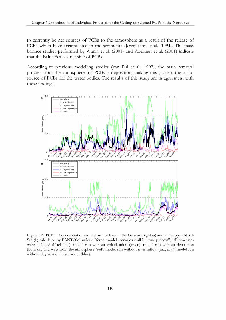
Chapter 6 Contribution of Individual Processes to the Cycling of Selected POPs in the North Sea
110
to currently be net sources of PCBs to the atmosphere as a result of the release of PCBs which have accumulated in the sediments (Jeremiason et al., 1994). The mass balance studies performed by Wania et al. (2001) and Axelman et al. (2001) indicate that the Baltic Sea is a net sink of PCBs.
According to previous modelling studies (van Pul et al., 1997), the main removal process from the atmosphere for PCBs is deposition, making this process the major source of PCBs for the water bodies. The results of this study are in agreement with these findings.
0
0.1
0.2
0.3
Con
cent
ratio
n (n
g/l)
A ug- 9
5
Nov-95
Feb-96
May -96
A ug- 9
6
Nov-96
Feb-97
May -97
A ug-97
Nov-97
Feb-98
May -98
A ug-98
Nov-98
Feb- 9
9
May -99
Aug-99
Nov-99
Feb- 0
0
May-00
Aug-00
Nov-00
Feb-01
May-01
Aug-01
Nov-01
everythingno volatilisationno degradationno atm depositionno rivers
0
0.2
0.4
0.6
Con
cent
ratio
n (n
g/l)
A ug- 9
5
Nov-95
Feb-96
May -96
A ug- 9
6
Nov-96
Feb-97
May -97
A ug-97
Nov-97
Feb-98
May -98
A ug-98
Nov-98
Feb- 9
9
May -99
Aug-99
Nov-99
Feb- 0
0
May-00
Aug-00
Nov-00
Feb-01
May-01
Aug-01
Nov-01
everythingno volatilisationno degradationno atm depositionno rivers
(a)
(b)
Figure 6-6: PCB 153 concentrations in the surface layer in the German Bight (a) and in the open North Sea (b) calculated by FANTOM under different model scenarios (“all but one process”): all processes were included (black line); model run without volatilisation (green); model run without deposition (both dry and wet) from the atmosphere (red); model run without river inflow (magenta); model run without degradation in sea water (blue).

Chapter 6 Contribution of Individual Processes to the Cycling of Selected POPs in the North Sea
111
In contrast to α-HCH, air concentrations of PCB 153 over the North Sea used in this study have not shown a fast decline. Although some localised trends may be apparent, overall, no obvious changes in PCB 153 levels in sea water have been established.
6.3.5 The role of temperature and wind speed in the air-sea gaseous exchange
It the previous section it has been shown that the gaseous air-sea flux plays a key role in controlling the fate of the three selected POPs in the North Sea. For the North Sea as a whole the net air-sea flux for γ- and α-HCH was depositional, whereas for the inner German Bight it is volatilisational. PCB 153 concentrations showed potential for net volatilisation in the entire North Sea. In the inner German Bight the air-sea flux remained net volatilisational during the entire simulation period.
Besides the non-equilibrium state between air and sea concentrations, the air-sea gaseous flux is also driven by the wind speed and temperature (see Sect. 2.2.1). It is believed that the wind speed determines the rate of the air-sea flux, whereas the temperature can have a significant role in determining the flux direction (Bidleman et al., 1995).
The fortnightly mean air-sea fluxes of γ-, α-HCH and PCB 153 were plotted together with the correspondent air, sea surface temperatures (SST) and wind speeds for the German Bight and for the open North Sea for the entire simulation period (Fig. 6-7).
The SST values calculated by HAMSOM (Sect. 3.2) lie in a range between 1°C and 20°C in the German Bight (Fig. 6-7a) and between 4°C and 15°C in the open North Sea (Fig. 6-7c) during the simulation period. The measured air temperatures have higher temporal gradients, dropping to negative values in winter 1996. The peaks in the SST occur generally after the peaks in air temperatures having the maxima of SST in late August and minima in February. The wind speeds are generally higher in winter season.
The values of the air-sea gaseous flux for γ-HCH range between -0.3⋅10-3 ng m-2 s-1 and +0.8⋅ 10-3 ng m-2 s-1 in the German Bight and 0.1⋅10-3 ng m-2 s-1 and 1.2⋅10-3 ng m-2 s-1 in the open North Sea. The air-sea flux of γ-HCH in the German Bight calculated for the 6 years revealed a clear seasonal pattern. In winter the air-sea flux of γ-HCH in the German Bight is volatilisational. In April until June it turns to net depositional. Later from July to October it turns to volatilisational again, turning back to depositional in October – December. The maxima in depositional flux often corresponded to the maxima in the wind speeds, i.e. in winter.
Chapter 6 Contribution of Individual Processes to the Cycling of Selected POPs in the North Sea
112
The air-sea exchange of γ-HCH both in the German Bight and in the open North Sea has gone to a near equilibrium state in 1999. Although the air-sea flux of γ-HCH in the open North Sea has a similar annual cycle as the one in the German Bight, it was net depositional throughout the whole simulation. This pattern is in agreement with the results of budget calculations (Sect 6.1.1).
The air-sea gaseous flux values for α-HCH ranges between -0.5⋅10-3 ng m-2 s-1 and +1.2⋅10-3 ng m-2 s-1 in the German Bight (Fig. 6.7b) up to 1.9⋅10-3 ng m-2 s-1 in the open North Sea (Fig. 6-7c). The model results suggest that the air-sea gaseous flux in the German Bight has a seasonal cycle: it is mostly volatilisational in winter, i.e. between December and February, than the flux turns to depositional in March and remains so until August with episodic volatilisation events. In August until October the volatilisation prevails, later on reversing to deposition. The air-sea flux of α-HCH in the North Sea was always depositional with a near equilibrium state in 2001.
The gaseous air-sea flux of PCB 153 during the studied period was in the range between -6⋅10-5 ng m-2 s-1 and 1.9⋅10-5 ng m-2 s-1 in the German Bight (Fig. 6.7b) and -5⋅10-5 ng m-2 s-1 and 2.1⋅10-3 ng m-2 s-1 in the open North Sea (Fig. 6-7c). These values are in agreement with the measurements based atmospheric deposition fluxes calculated for the eastern Skagerak (Palm et al., 2003) which were in 5.5 ng m-2 day-1 in summer and 0.57 ng m-2 day-1 in winter. The model predicts that volatilisation of PCB 153 occurred during spring although there was no clear seasonal cycle.
The major difference between the air-sea fluxes of two HCHs and PCB 153 is that volatilisation of PCB 153 also occurs in the open North Sea, whereas the HCHs volatilise in the German Bight. The temperature dependency of the air-sea flux was the process which is thought to be least certain under present model setup. The temperature dependency of the HLC was shown to be a very significant factor determining the magnitude and direction of the air-sea flux (see Chapter 4). The choice of different HLC values altered the HCH concentration by 50%. Such experiments were not performed for PCB 153 because of the lack of data on the HLC dependency on temperature.

Chapter 6 Contribution of Individual Processes to the Cycling of Selected POPs in the North Sea
113
Jan-96 Jul-96 Jan-97 Jul-97 Jan-98 Jul-98 Jan-99 Jul-99 Jan-00 Jul-00 Jan-01 Jul-01 Jan-02-50
10
20
30
Tem
pera
ture
, 0 C
0
5
10
15
Win
d S
peed
, m s
- 1
Jan-96 Jul-96 Jan-97 Jul-97 Jan-98 Jul-98 Jan-99 Jul-99 Jan-00 Jul-00 Jan-01 Jul-01 Jan-02-1
0
1
2x 10
-3
Flux
, ng
m-2
s-1
-6
-4
-2
0
2
4
Flux
, ng
m-2
s-1
Jan-96 Jul-96 Jan-97 Jul-97 Jan-98 Jul-98 Jan-99 Jul-99 Jan-00 Jul-00 Jan-01 Jul-01 Jan-020
1
2
3x 10
-3
Flux
, ng
m-2
s-1
-6
-4
-2
0
2
4
Flux
, ng
m-2
s-1
Jan-96 Jul-96 Jan-97 Jul-97 Jan-98 Jul-98 Jan-99 Jul-99 Jan-00 Jul-00 Jan-01 Jul-01 Jan-02-50
10
20
30Te
mpe
ratu
re, 0 C
0
5
10
15
Win
d S
peed
, m s
- 1
Tair Tsea WS
Tair Tsea WS
Fa-w for γ-HCH Fa-w for α -HCH Fa-w for PCB 153
Fa-w for γ-HCH Fa-w for α -HCH Fa-w for PCB 153
(a)
(b)
(c)
(d)
x 10-5
x 10-5
German Bight
open North Sea
Figure 6-7: Fortnightly means of measured air temperature and sea surface temperature calculated by HAMSOM (a) in the German Bight (location A) and (c) in the open North Sea (location M) and the correspondent gaseous air-sea fluxes of γ-, α-HCH and PCB 153 in ng m-2 s-1 (b) and (d) calculated by FANTOM.

Chapter 6 Contribution of Individual Processes to the Cycling of Selected POPs in the North Sea
114

Chapter 7 Conclusions and Outlook
115
Chapter 7
Conclusions and Outlook
7.1 Conclusions Persistent organic pollutants are harmful to human health and the environment. However their fate and pathways in the different environmental compartments are not yet fully understood. Models of POPs are recognised as helpful tools for assessing their cycling in natural systems. Model application is encouraged under the Convention on LRTAP and the Stockholm Convention. The objective of this thesis was to advance the understanding of the fate of POPs in the aquatic environment as basis for realistic estimates of their spatial and temporal distribution and pathways in the North Sea. With such information current and future exposure of the North Sea to contamination by POPs can be addressed.
In chapter 2 the fate and transport ocean model FANTOM developed to assess the fate of POPs in the North Sea is described. FANTOM is based on the state-of-the-art knowledge about the mechanisms governing POPs behaviour in sea water. Considered processes are transport with sea currents, atmospheric deposition and air-sea exchange, degradation in sea water, partitioning to particles suspended in sea water and subsequent sedimentation or resuspension from the bottom. In other POPs models settling with particles in the oceanic compartment is treated as an ultimate sink. Recent measurements in the North Sea (van der Zee and Chou, 2005) showed that resuspended sediments can have a significant contribution to the POC load in sea water. The resuspension of previously settled POC has been considered in FANTOM.
In chapter 3 the model setup for investigating the sea water fate of γ-HCH, α-HCH and PCB 153 in the North Sea during the years 1995-2001 is presented. For the first time a measurement based ocean model is applied on the regional scale. The three pollutants were chosen based on the differences in their physical-chemical properties (and consequently environmental behaviour) and data availability on the time scales of several years. To assure a realistic representation of POPs fate in sea water, a survey on physical-chemical properties and available observational data was performed.

Chapter 7 Conclusions and Outlook
116
• The physical-chemical properties in some cases can differ in more than one or even two orders of magnitude. Recently reported physical-chemical properties were chosen for the model calculations.
• The compilation of observational data on POPs in the North Sea substances revealed that although it is relatively well assessed comparing to other seas, data for sea water are sparse in time and space. The data sets for γ- and α-HCH were the best in terms of spatial and temporal coverage. Measured sea water concentrations of PCB 153 are low and were often very close or below the detection limit.
In chapter 4 modelled γ-HCH, α-HCH and PCB 153 concentrations in the surface water were compared with the measured ones at different locations in the North Sea. No measurements of the vertical concentration profiles were available. As far as comparison was possible, it was found that FANTOM is able to reproduce the spatial distribution of γ-HCH, α-HCH and PCB 153 concentrations in sea water.
Gradual decrease in α-HCH sea water concentrations and increase in γ-HCH until 1998 with subsequent decrease in the 1998-2001 concentrations were captured by the model. The decrease predicted for the central part of the North Sea for both HCHs is slower than the one for the areas remote from the polluted estuaries. In most of the compared location there is a good correlation between observations and the model results with correlation coefficient values up to 0.95. Weaker correlation was found for the colder periods when calculated concentrations were higher than observed. This is due to insufficient temporal resolution of the observational time series and due to the uncertainties in the temperature dependency of HLC (Henry’s law constants) used for the air-sea flux calculations. The latter hypothesis was verified by the model experiments using two different temperature dependencies of HLC for γ- and α-HCH. These model experiments revealed:
• Different HLC temperature dependencies are responsible for 20-50% change in γ-HCH and in up to 60% change in α-HCH sea water concentrations.
A model experiment with boundary conditions set up at the lateral boundaries showed:
• Overestimations in the modelled concentrations of γ-HCH in 2000-2001 seem to be due to insufficient input data at the open sea boundaries.
• Inflows from the English Channel and the Atlantic Ocean at the northern boundary contribute to the loads of γ-HCH even in the German Bight. However this contribution seems to be decreasing now.

Chapter 7 Conclusions and Outlook
117
• A similar experiment for α-HCH showed that its transport through the oceanic boundaries is less significant for the levels of α-HCH in the North Sea than for γ-HCH.
The model captures the spatial and temporal gradients of the concentration for HCHs as well as the concentration range for PCB 153, although correlations between observed and modelled concentrations were not higher than 0.7 which is lower than for the two HCHs. Also the observational data for PCB 153 are more uncertain due to its low concentrations in sea water. The model results suggest that the predicted PCB 153 pattern is determined by the input data variability. No clear temporal trend for PCB 153 is detected.
Concentrations in the atmosphere correlate with concentrations in sea water, indicating the significance of the atmospheric input of γ-HCH, α-HCH and PCB 153 in the North Sea. Although the air-sea exchange is one of the most important driving mechanisms, it also introduces major variability in the model results.
In chapter 5 occurrence of γ-HCH, α-HCH and PCB 153 and their pathways within the North Sea were studied. The model results showed:
• Partitioning to suspended particles in sea water is expected to be most important for PCB 153 as it is the most lipophilic pollutant addressed in this study. FANTOM estimates that up to 90% of the total PCB 153 concentration can be in particulate form. For the two HCHs this fraction is below 2%. A correlation between the annual cycle of biomass and PCB 153 sea water concentrations is predicted.
• The temporal pattern of modelled concentrations of the three pollutants in sea water is also reflected in fish concentrations of these POPs. Although PCB 153 sea water concentrations were up to two orders of magnitude lower than the concentrations of γ-HCH and α-HCH, the levels in fish for PCB 153 are up to two orders of magnitude higher than those of HCHs. The expected bioaccumulation potential of PCB 153 is confirmed. This implies that even very low concentrations of PCB 153 in sea water are still hazardous for the North Sea ecosystem.
• The vertical distributions of γ-HCH, α-HCH predicted by FANTOM follow the water mass stratification, i.e. well mixed from the surface to the bottom in winter and stratified due to thermal stratification in summer. In case of PCB 153, the vertical concentration is shaped by the dynamics of POC when there are sufficiently high concentrations of POC available and by water mass stratification otherwise.

Chapter 7 Conclusions and Outlook
118
• The calculated α/γ-HCH ratio shows no pronounced trend during the simulation period. The ratio values remained low (<0.5) nearly in the entire modelling domain indicating the predominance of sources of lindane in the region.
In chapter 6 the contribution of individual processes to the abundance of γ-HCH, α-HCH and PCB 153 was assessed. The annual mass budgets and residence times of these three pollutants were presented. The entire North Sea (within the modelling domain) was compared to the inner German Bight.
• Atmospheric deposition and rivers are the two largest sources of γ-HCH, α-HCH and PCB 153 (for the system). The relative importance of these sources is different for the German Bight and the North Sea as a whole. Atmospheric deposition contribution to the loads of the three selected contaminants was up to 85% in the North Sea (entire modelling domain) and below 45% in the German Bight. Air-sea flux and transport with sea currents are the major mechanisms which determine the cycling of the three POPs in the North Sea.
• According to the annual budgets, the net air-sea gaseous flux is depositional in the whole North Sea for γ- and α-HCH. This is consistent with findings of POPCYCLING-Baltic project (Pacyna et al. 1999), the air-sea flux of α-HCH was found depositional in Skagerrak in 1980-2000. FANTOM predicts volatilisational flux of γ- and α-HCH in the inner German Bight. For PCB 153 it was both net depositional and volatilisational for individual years in the two compared regions. Measurements in the Baltic Sea showed that with regard to PCBs temperature dependency of the HLC can significantly alter the air-sea flux magnitude and direction (Bruhn et al., 2003). This means that the choice of HLC introduces significant uncertainties to the calculated gaseous fluxes of PCB 153. A similar effect can be expected for HCHs based on test runs using another HLC temperature dependency.
• The contribution of water to POC partitioning of γ-HCH, α-HCH and PCB 153 to the budgets is also distinguished. This is probably due to the relatively high content of POC in the North Sea compared to the global ocean. Even for such a fairly water soluble compound as α-HCH the sinking flux of POC associated fraction has the same order of magnitude as the river inflow. According to the model calculations, POC resuspension returns up to 80% of the previously deposited contaminants.

Chapter 7 Conclusions and Outlook
119
7.2 Outlook
Measurements of most POPs in sea water are still too limited (maybe with the exception of HCH isomers) to allow comprehensive assessment of their spatial and temporal distributions. Therefore models have to be further developed and used to assess their sources and establish their environmental effects.
From this study, it has become clear that transport models can address the fate of some POPs, at least on the regional scale. Despite the uncertainties in some input parameters and lack of observational data, FANTOM was capable to reproduce realistic multi-year temporal and spatial distributions of γ-HCH, α-HCH and PCB 153 in the North Sea and even can indicate their concentrations in biota (fish tissue).
The model in present developmental stage can be used for several purposes.
• Evaluating “new” substances, for accessing the impact of historical (past time) emissions in the present conditions of the North Sea.
• Evaluating import (influence of discharges of other countries to contamination in waters of a given country) and export (influence of discharges of each country to contamination of coastal waters of other countries) of a certain POP. Moreover, if atmospheric depositions can be allocated to countries, the import and export evaluation can be performed with regard to atmospheric emission of these countries too.
• Elaborating case studies for possible scenarios. For example scenarios of economic development and related usage of coastal and marine environments.
• To address the effects of climate change and variability in the 21st century. Climate change and variability can have profound effects on the pathways of POPs globally and in the North Sea in particular, both in response to physical and biological factors. Ocean currents, the air-sea exchange of POPs are all subject to alteration as a result of climate change. Therefore the current exposure of the North Sea to contamination of POPs could alter dramatically as climate-related physical and biological phenomena change over the coming decades.
The modelling concept developed and applied in this study is also valid for simulating the fate of other contaminants in the North Sea which do not behave as passive tracers, e.g. radioactive substances or heavy metals. FANTOM can be also applied to other seas, e.g. the Baltic Sea or the Irish Sea.
The most significant gaps to fill for future development and application of POPs fate models are:

Chapter 7 Conclusions and Outlook
120
• Improvement of input parameters including both observational data and compounds physical-chemical properties. This refers first of all to HLC as it is the most important for model applications in the marine environment.
• Refined description of the key processes. This applies first of all to the air-sea flux parameterisation which is one of the major mechanisms driving the POPs fate in aquatic systems, but is so far incompletely described, e.g. effect of rain, spray drops, surface films. For example, volatilisation could be limited by the presence of organic films. This would significantly change the budgets of PCB 153 (Fig. 6-6).
In conclusion, it remains a future task to investigate the fate of compounds with different environmental behaviour. This model could be the base for further research on the contribution of different sources and sinks and sensitivity of contaminants behaviour in the marine environment to the individual processes under present and future climate conditions.

Appendix A
121
Appendix A
Table A-1: Parameters used in FANTOM.
Parameter Symbol Units Value, reference
γ-HCH α-HCH PCB 153
Molar mass M g mol-1 290.85 360.88
10.14 ± 0.55 [1] 10.13 ± 0.29 [1] Intercept of the temperature dependent Henry’s law constant
b - 7.54 ± 0.54 [2] 9.31 ± 0.38 [2]
14.05 [4]
- 3208 ± 161 [1] -3098 ± 84 [1] Slope of the temperature dependent Henry’s law
constant m K
- 2382 ± 160 [2] -2810 ± 110 [2] -3662 [4]
Octanol-water partitioning coefficient owK - 3.98×10³ [3] 5.89×10³ [3] 5.62×10⁶ [5]
Degradation rate in ocean water at 298 K degk s-1 2.3×10⁻⁸ [3] 2.7×10⁻⁸ [3] 1.6×10⁻⁹ [5]
Dry particle deposition velocity depv m s-1 2×10⁻⁵ [6], [7]
Specific aerosol surface θ m2 m-3 1.5×10⁻⁴ [8]
Adsorption constant s Pa m 0.17 [9]
Settling velocity of SPM setv m s-1 3×10⁻⁴ [10]
Threshold shear velocity for erosion of SPM
ecr,*v m s-1 0.028 [10]
Threshold shear velocity for deposition of SPM
dcr,*v m s-1 0.01 [10]
[1] Sahsuvar et al., 2003; [2] Kucklick et al., 1991; [3] Klöpffer and Schmidt, 2001; [4] Paasivitra et al., 1999; [5] Beyer et. al., 2001; [6] McMahon and Denison, 1979; [7] Slinn, 1983; [8] Pekar et al., 1998; [9] Junge, 1977; [10] Pohlmann and Puls, 1994

Appendix B
122
Appendix B
Table B-1: List of stations used for the model results evaluation, their geographical locations and number of measurements available for γ-HCH, α-HCH and PCB 153 within the simulation period (1995-2001).
Symbol on the map
Lat. Long. Months of sampling
Number of measurements γ-
HCH
Number of measurements
α-HCH
Number of measurements PCB
153
A 54.00o N 8.00o E 5-9 36 36 31
B 53.72o N 7.45o E 11-2 14 14 14
C 53.85 o N 8.06 o E 11-2 14 14 14
D 53.86 o N 8.13 o E 11-2 14 14 14
E 53.98 o N 8.22 o E 11-3, 5, 7-9 26 14 14
F 54.05 o N 7.86 o E 11-2 14 14 14
G 54.22 o N 8.38 o E 1, 2, 5-9 41 40 21
H 54.25 o N 7.50 o E 5-9 25 30 17
I 54.67 o N 6.33 o E 5-9 20 17 10
J 55.00 o N 6.25 o E 5-8 12 17 9
K 55.00 o N 8.25 o E 5-9 21 25 22
L 55.50 o N 4.17 o E 5, 9, 12 18 23 0
M 56.00 o N 3.00 o E 7 4 0 0
N 52.58 o N 3.53 o E 2, 3, 5, 8, 11, 12 21 22 0
O 51.96 o N 2.68 o E 2, 5, 8, 11 7 7 0
P 54.42 o N 4.04 o E 8 6 6 0
Q 55.00 o N 6.20 o E 9, 10 8 8 6
R 55.00 o N 8.00 o E 5,6 8,9 7 7 0
Total number of measurements: 308 308 186

List of Figures
123
List of Figures
Figure 1-1: Distribution of γ-HCH concentrations (ng/l) in surface water in 1995 based on measurements campaigns. Source: OSPAR (2000).
Figure 1-2: Temporal trend of α- and γ-HCH concentrations in surface water of the German Bight (Station T 41) since 1986. Source: BSH (2005).
Figure 2-1. Diagram to illustrate key processes affecting POPs fate included in FANTOM.
Figure 3-1: FANTOM domain and bathymetry (depth in m) on a grid of 1.5’×2.5’ (corresponding to 2.5–3 km). Locations of stations where measurements of γ-HCH atmospheric concentrations were available are indicated in red (Lista lies outside of the modelling domain). Rivers mouths are indicated in green (the rivers Rhine and Meuse drain into the North Sea through Ijssel, Nordzeekanaal, Nieuwe Waterweg and Haringvliet).
Figure 3-2: Diagram of general circulation in the North Sea. The width of arrows indicates the magnitude of volume transport; red arrows indicate Atlantic water. Source: Turrell et al. (1992).
Figure 3-3: The input-output diagram for the integration of HAMSOM and FANTOM.
Figure 3-4: Categorisation of the behaviour of organic substances as a function of their distribution characteristics defined by the physical-chemical properties: air-water and octanol-air partition coefficients. Four different behaviour categories are identified and assigned sections of the diagram: “no hop” – chemicals that are so volatile that they do not deposit to the Earth’s surface and thus remain in the atmosphere; ‘multi-hop” – chemicals that readily shift their distribution between gas phase and condensed phase (soil, vegetation, water) in response to changes in environmental temperature and phase composition, and therefore can travel long distances in repeated cycles of evaporation and deposition; “single hop” – chemicals that are so involatile or so water-insoluble that they can undergo LRT only by piggybacking on suspended solids

List of Figures
124
in air and water; “no hop required” – chemicals that are sufficiently water soluble to undergo long range transport by being dissolved in the water phase. (Adapted from UNEP Global Report 2003).
Figure 3-5: Initial distribution of γ-HCH concentration (ng/l) in the North Sea in the summer, 1995: points-measurements, colours-interpolated field.
Figure 3-6: Initial distribution of α-HCH concentration (ng/l) in the North Sea in the summer, 1995: points-measurements, colours-interpolated field.
Figure 3-7: Initial distribution of PCB 153 concentration (ng/l) in the North Sea in the summer, 1995: points-measurements, colours-interpolated field.
Figure 3-8: a) γ-HCH concentrations in the atmosphere at the EMEP stations and b) γ-HCH loads (Qriv x Criv) in the continental rivers. Geographical locations of the measurement sites are shown on the map (Fig. 3-1).
Figure 3-9: a) α-HCH concentrations in the atmosphere at the EMEP stations and b) α-HCH loads in the continental rivers.
Figure 3-10: a) PCB 153 concentrations in the atmosphere at the EMEP stations and b) PCB 153 loads in the continental rivers.
Figure 4-1: FANTOM modelling domain and geographical locations of points where observation time series were available for the model evaluation (labelled with letters). Data for points A to M were provided by the German Oceanographic Centre (DOD, 2005) covering only the German exclusive economic zone of the North Sea. Data for points P, N and O are from the Dutch database Waterbase (DONAR, 2005). Stations where measurements of γ-HCH, α-HCH and PCB 153 atmospheric concentrations were available are indicated in red (Lista lies outside of the modelling domain). Rivers mouths are indicated in green.
Figure 4-2: Observed (dots) and calculated by FANTOM (solid line) γ-HCH concentrations (ng/l) in the surface layer at the locations D, G, H, F. Geographical locations of points are given in Table B-1 and shown on Fig. 4-1.
Figure 4-3: Observed (dots) and calculated by FANTOM (solid line) γ-HCH concentrations (ng/l) in the surface layer at the locations J, L, P, K. Geographical locations of points are given in Table B-1 and shown on Fig. 4-1.
Figure 4-4: Measured vs. calculated γ-HCH concentrations (ng/l) in the surface layer at the locations A, G, K, L, N, P. Geographical locations of points are given in Table B-1 and shown on Figure 4-1.

List of Figures
125
Figure 4-5: Measured vs. calculated γ-HCH concentrations (ng/l) in the surface layer in all locations. Number of measurements is 308.
Figure 4-6: Observed (dots) and calculated by FANTOM (solid line) α-HCH concentrations (ng/l) in the surface layer at the locations D, G, H, F. Geographical locations of points are given in Table B-1 and shown on Fig. 4-1.
Figure 4-7: Observed (dots) and calculated by FANTOM (solid line) α-HCH concentrations (ng/l) in the surface layer at the locations J, L, P, K. Geographical locations of points are given in Table B-1 and shown on Fig. 4-1.
Figure 4-8: Measured vs. calculated α-HCH concentrations (ng/l) in the surface layer in all locations. Number of measurements is 308.
Figure 4-9: Observed (dots) and calculated by FANTOM (solid line) PCB 153 total concentrations (ng/l) in the surface layer at the locations A, H, J, L. Geographical locations of points are given in Table B-1 and shown on Fig. 4-1.
Figure 4-10: Measured vs. calculated PCB 153 concentrations (ng/l) in the surface layer in all locations. Number of measurements is 186.
Figure 4-11: Concentrations of PCB 153: blue line – model simulation in the German Bight at the location E; green – concentration supplement form the River Elbe; red – individual measurements at the location E.
Figure 4-12: Observed (dots) and calculated by FANTOM (solid lines) γ-HCH concentrations (ng/l) in the surface layer at the location A and N, under different model setup: blue line – main model simulation; magenta line – when γ-HCH concentrations inflowing via the lateral boundaries were equal zero; green – when air-sea exchange was calculated using Henry’s law constants given by Kucklick et al. (1991). Geographical location is given in Table B-1 and shown on Fig. 4-1.
Figure 4-13: Observed (dots) and calculated by FANTOM (solid lines) α-HCH concentrations (ng/l) in the surface layer at the location A and N, under different model setup: blue line – main model simulation; magenta line – when α-HCH concentrations inflowing via the lateral boundaries were equal zero; green – when air-sea exchange was calculated using Henry’s law constants given by Sahsuvar et al. (2003). Geographical location is given in Table B-1 and shown on Fig. 4-1.
Figure 5-1: FANTOM domain and the vertical sections location (brown line) along 3°E presented in this chapter. Geographical locations of points where temporal trends were presented are labelled with letters. Rivers mouths are indicated in green.
List of Figures
126
Figure 5-2: Vertically integrated concentrations (mg/l) of particulate organic carbon: (a) and (c) due to biological activity in winter and summer 1996 respectively provided by Pätsch and Kühn, (2005); (b) and (d) are POC concentrations originating from bottom sediment in winter and summer 1996 respectively calculated by FANTOM.
Figure 5-3: Surface daily averaged concentrations of total particulate organic carbon CPOC (blue line) in 1996, consisting of primary production, Cbio (green line) (Pätsch and Kühn, 2005) and of resuspended fraction, Csed (brown line) calculated by FANTOM (a) in the German Bight (location A) and (b) in the open North Sea (location L).
Figure 5-4: Distributions of vertically integrated annual mean POPs fraction on POC (%) of (a) γ-HCH, (b) α-HCH and (c) PCB 153 and (d) vertically averaged total POC annual mean concentration (mg/l).
Figure 5-5: Vertical sections from south to north along 3oE (see Fig. 5-1) of annual mean POPs fraction on POC (%) of (a) γ-HCH, (b) α-HCH and (c) PCB 153 and (d) annual mean total POC concentration (mg/l).
Figure 5-6: PCB 153 total C and bound to particles pC concentrations at the sea surface: (a) in the German Bight (location A) and (b) in the open North Sea (location L).
Figure 5-7: The North Sea flatfish dab (Limanda Limanda). Source: Natural History Museum (2005).
Figure 5-8: Concentrations of γ-HCH, α-HCH and PCB 153 in flatfish dab liver (median values of individual measurements provided by the Institut für Fischereiökologie) measured in the German Bight (bars) and vertically integrated annual mean modelled by FANTOM sea water concentrations in the same location (dashed line).
Figure 5-9. Vertical sections from south to north along 3°E of sea temperature (colours, °C) and salinity (lines) in January (a) and August (c) 1997 calculated by HAMSOM and corresponding γ-HCH total concentrations (ng/l) (b and d) calculated by FANTOM.
Figure 5-10: Vertical sections from south to north along 30E of α-HCH total concentrations in January (a) and August (b) 1997 calculated by FANTOM.
Figure 5-11: Vertical sections from south to north along 3°E of PCB 153 total concentrations (ng/l) in January (a) and August (b) 1997 calculated by FANTOM.

List of Figures
127
Figure 5-12: Vertically integrated annual mean concentrations of γ-HCH (ng/l) in the North Sea calculated by FANTOM.
Figure 5-13: Vertically integrated annual mean concentrations of α-HCH (ng/l) in the North Sea calculated by FANTOM.
Figure 5-14: Vertically averaged annual mean concentrations of PCB 153 (ng/l) in the North Sea calculated by FANTOM.
Figure 5-15: Monthly mean α/γ-HCH ratio (based on surface concentrations) in sea water in January (a) and July (b) 1997 calculated by FANTOM.
Figure 5-16: α/γ-HCH concentration ratio in sea water at the locations A, J, L, N. Solid lines are model results derived from the main runs for α-HCH and γ-HCH; dashed lines are derived from observations.
Figure 6-1: Modelling domain of FANTOM and the boundaries of the inner German Bight (brown lines) selected for the budgets calculations.
Figure 6-2: Cumulative masses (kg) calculated by FANTOM (for entire modelling domain, for each year) for γ-HCH (a), α-HCH (b) and PCB 153 (c) contributed by different processes acting in sea water as sources, i.e.: dry and wet atmospheric deposition, resuspension from the sea bottom, rivers inflow, inflow from the Atlantic Ocean (through the northern boundary) and from the English Channel (southern boundary); or sinks, i.e.: volatilisation, sinking to the sea bottom, degradation, outflow through the northern and southern boundaries.
Figure 6-3: Cumulative masses (kg) calculated by FANTOM (for the inner German Bight, for each year) for γ-HCH (a), α-HCH (b) and PCB 153 (c) contributed by different processes acting in sea water as sources, i.e.: dry and wet atmospheric deposition, resuspension from the sea bottom, rivers inflow, inflow through the western and the northern boundaries or sinks, i.e.: volatilisation, sinking to the sea bottom, degradation and outflow through the northern and western boundaries.
Figure 6-4: γ-HCH concentrations in the surface layer in the German Bight (a) and in the open North Sea (b) calculated by FANTOM under different model scenarios (“all but one process”): all processes were included (black line); model run without volatilisation (green); model run without deposition (both dry and wet) from the atmosphere (red); model run without river inflow (magenta); model run without degradation in sea water (blue).
Figure 6-5: α-HCH concentrations in the surface layer in the German Bight (a) and in the open North Sea (b) calculated by FANTOM under different model scenarios (“all

List of Figures
128
but one process”): all processes were included (black line); model run without volatilisation (green); model run without deposition (both dry and wet) from the atmosphere (red); model run without river inflow (magenta); model run without degradation in sea water (blue).
Figure 6-6: PCB 153 concentrations in the surface layer in the German Bight (a) and in the open North Sea (b) calculated by FANTOM under different model scenarios (“all but one process”): all processes were included (black line); model run without volatilisation (green); model run without deposition (both dry and wet) from the atmosphere (red); model run without river inflow (magenta); model run without degradation in sea water (blue).
Figure 6-7: Fortnightly means of measured air temperature and sea surface temperature calculated by HAMSOM (a) in the German Bight (location A) and (c) in the open North Sea (location M) and the correspondent gaseous air-sea fluxes of γ-, α-HCH and PCB 153 in ng m-2 s-1 (b) and (d) calculated by FANTOM.

Bibliography
129
Bibliography
AMAP Assessment Report: Arctic Pollution Issues: Arctic Monitoring and Assessment Programme. Oslo, Norway, 1998.
Axelman, J., Broman, D., Näf, C.: Field measurements of PCB between water and planktonic organisms: influence of growth, particle size, and solute-solvent interactions, Environ. Sci. Technol., 31, 665-669, 1997.
Axelman, J., Broman, D.: Budget calculations for polychlorinated biphenyls (PCBs) in the Northern Hemisphere - a single-box approach. Tellus B, Volume 53, Number 3, 235-259(25), 2001.
Baart, A., Berdowski, J., van Jaarsveld, J., Wulffraat, K.: Calculation of atmospheric deposition of contaminants on the North Sea. TNO-MEP-R 95/138, Delft, The Netherlands, 1995.
Backhaus, J. O.: A three-dimensional model for the simulation of shelf sea dynamics, Deutsche Hydrographische Zeitschrift, 38, 167-187, 1985.
Bartels, J.: Gezeitenkräfte, Handbuch der Physik, Band XLVIII, Geophysik, II, 1957.
Baumert, H., Simpson, J., Sündermann, J. (Eds.): Marine Turbulence - Theories, Observations and Models, Cambridge University Press, 652 pp., 2005.
Bethan, B., Dannecker, W., Gerwig, H., Hühnerfuss, H., Schulz, M.: Seasonal dependence of the chiral composition of alpha-HCH in coastal deposition at the North Sea. Chemosphere, 44(4), 591-597, 2001.
Beyer, A., Matthies, M.: Long-Range Transport Potential of Semivolatile Organic Chemicals in Coupled Air-Water Systems. Environ. Sci. Poll. Res. 8, 173-179, 2001.
Bidleman, T. F.: Atmospheric process, Environ. Sci. Technol., 22, 361-367, 1988.
Bidleman, T. F., Jantunen, L. M., Falconer, R. L., Barrie, L. A., Fellin, P.: Decline of hexachlorocyclohexane in the arctic atmosphere and reversal of air-sea gas exchange, Geophys. Res. Lett., 22(3), 219-222, 10.1029/94GL02990, 1995.

Bibliography
130
Breivik, K., Pacyna, J.M., Münch, J.: Use of alpha-, beta- and gamma-hexachlorocyclohexane in Europe, 1970-1996. Science Total Environ. 239, 151-163, 1999.
Bruhn, R., Lakaschus S., McLachlan, M., S.: Air/sea gas exchange of PCBs in the southern Baltic Sea, Atmospheric Environment, 37(24), 3445-3454, 2003.
BSH: Nordseezustand 2003. Authors: Loewe, P., Schmolke, S., Becker, G., Brockmann, U., Dick, S., Engelke, C., Frohse, A., Horn, W., Klein, H., Müller-Navarra., S., Nies, H., Schmelzer, N., Schrader, D., Schulz, A., Theobald, N., Weigelt, S., Berichte des BSH No38, 2005.
Chernyak, S. M., Rice, C. P., McDonnell, L. L.: Evidence of Currently-Used Pesticeds in Air, Ice, Fog, Seawater and Surface Microlayer in the Bering and Chukchi Seas. Marine Pollution Bulletin, 32, 410-419, 1996.
Coulston, F., and Kolbye, A. (Eds.): Regulatory Toxicology and Pharmacology, vol. 20, no. 1, part 2, 1994.
Dachs, J., Lohmann, R., Ockenden, W.A., Mejanelle, L., Eisenreich, S.J, Jones, K.C.: Oceanic biogeochemical controls on global dynamics of persistent organic pollutants. Environ. Sci. Technol., 36, 4229-4237, 2002.
DOD: German Oceanographic Data Centre, http://www.bsh.de/, 2005.
DONAR: Dutch online database Waterbase, http://www.waterbase.nl/, 2005.
Eisma, D., Kalf, J.: Distribution, organic content and particle size of suspended matter in the North Sea, Netherlands Journal of Sea Research 21(4), 265-285, 1987.
EMEP: Proceedings of the First Workshop on Emissions and Modelling of Atmospheric Transport of Persistent Organic Pollutants and Heavy Metals. Durham, N.C., United States, 6-7 May 1993. Editors: Pacyna, J.M., Voldner, E., Keeler, G.J., Evans, G. Lillestrøm, Norwegian Institute for Air Research (EMEP/CCC-Report 7/93), 1993.
EMEP: EMEP Data Online, http://www.emep.int/, 2005.
EU TGD, 1996. Technical Guidance Document in support of Commission Directive 93/67/EEC on Risk Assessment for new notified substances, Commission Regulation (EC) No 1488/94 on Risk Assessment for existing substances and Directive 98/8/EC of the European Parliament and of the Council concerning the placing of biocidal products on the market. European Chemicals Bureau, ISPRA.

Bibliography
131
Gaul, H.: Der Eintrag von Organohalogenverbindungen über die Atmosphäre in die Nordsee. Deutsche Hydrographische Zeitschrift, 36, 191-212, 1988.
Goldberg, E. D.: Synthetic organohalides in the sea. Proceedings of the Royal Society London, Series B 189, 277-289, 1975.
Gunnarsson J, Broman D, Jonsson P, Olsson M, Rosenberg R.: Interactions between eutrophication and contaminants: towards a new research concept for the European aquatic environment. Ambio, 24: 383-385, 1995.
Haarich, M.; Theobald, N.; Bachor, A.; Weber, M.v.; Grünwald, K.; Petenati, T.; Schröter-Kermani, C.; Jansen, W.; Bladt, A.: Organische Schadstoffe. Messprogramm Meeresumwelt (Heft 4): Zustandsbericht 1999–2002 für Nordsee und Ostsee. Hamburg und Rostock: Bundesamt für Seeschifffahrt und Hydrographie (Hrsg.), 195-218, ISSN 1611-2059, 2005.
Hansen, K. M., Christensen, J. H., Brandt, J., Frohn, L. M., Geels, C.: Modelling atmospheric transport of persistent organic pollutants in the Northern Hemisphere with a 3-D dynamical model: DEHM-POP. Atmos. Chem. Phys. Discuss., 4, 1339-1369, 2004.
Hargrave, B. T., Vass, W. P., Erickson, P. E.: Atmospheric transport of organochlorines to the Arctic Ocean. Tellus 40B: 480-493, 1988.
Haugen, J. E., Wania, F., Ritter, N, Schlabach, M.: Hexachlorocyclohexanes in air in Southern Norway. Temporal variation, source allocation, and temperature dependence, Environ. Sci. Technol., 32, 2, 217-224, 1998.
Hoff, R. M., Muir, D. C. G., Grift, N. P.: Annual Cycle of Polychlorinated Biphenyls and Organohalogen Pesticides in Air in Southern Ontario. 1. Air Concentration data. Environ. Sci. Technol., 26(2), 266-275, 1992.
Hornbuckle, K. C., Achman, D. R., Eisenreich, S. J.: Over-water and over-land polychlorinated biphenyls in Green Bay, Lake Michigan, Environ. Sci. Technol., 27(1): 87-98, 1993.
Hornbuckle, K. C., Jeremiason, J. D., Sweet, S. W., Eisenreich, S. J.: Seasonal variation in air-water exchange of polychlorinated biphenyls in Lake Superior. Environ. Sci. Tech., 28, 1491-1501, 1994.
Hühnerfuss, H., Bester, K., Landgraff, O., Pohlmann, T., Selke, K.: Annual balances of hexachlorocyclohexanes, polychlorinated biphenyls, and triazines in the German Bight. Mar. Pollut. Bull., 34, 419-426, 1997.
Bibliography
132
Iwata, H., Tanabe, S., Sakai, N. and Tatsukawa, R.: Distribution of persistent organochlorines in the oceanic air and surface seawater and the role of ocean on their global transport and fate, Environ. Sci. Technol., 27, 1080–1098, 1993.
Jacobs, C. M. J., van Pul, W. A. J.: Long-range atmospheric transport of persistent organic pollutants, I: Description of surface - atmosphere exchange modules and Implementation in EUROS. National institute of public health and the environment, Bilthoven, the Netherlands. Report No722401013, 1996.
Jantunen, L.M., Bidleman, T.F.: Air-water gas exchange of hexachlorocyclohexanes (HCHs) and the enantiomers of α-HCH in Arctic regions, Journal of Geophysical Research 101, 28837-28846, 1996 (corrections 102, 19279-19282, 1997).
Jaward, F. M., Barbera, J. L., Booijb, K., Jones, K. C.: Spatial distribution of atmospheric PAHs and PCNs along a north–south Atlantic transect, Environ. Pollut. 132: 173-181, 2004.
Jeremiason, J. D., Hornbuckle, K. C., Eisenreich, S. J.: PCBs in Lake Superior, 1978–1992: Decreases in water concentrations reflect loss by volatilization. Environ. Sci. Technol., 28, 903–914, 1994.
Jeremiason, J. D., Eisenreich, S. J., Paterson, M. J., Beaty, K. G., Hecky, R., Elser, J. J.: Biogeochemical Cycling of PCBs in Lakes of Variable Trophic Status: A Paired-Lake Experiment. Limnology and Oceanography, 44(3), 889-902, 1999.
Jones, K. C., de Voogt, P.: Persistent Organic Pollutants (POPs): state of the science. Environ. Poll., 100, 209-221, 1999.
Junge, C. E.: Basic considerations about trace constituent in the atmosphere is related to the fate of global pollutant. In: Fate of pollutants in the air and water environment. Part I, I.H. Suffet (ed.), John Wiley & Sons, New York, 484 pp, 1977.
Jurado, E., Lohmann, R., Meijer, S., Jones, K.C., Dachs, J.: Latitudinal and seasonal capacity of the surface oceans as a reservoir of PCBs. Environ. Pollut. 128: 149-162, 2004.
Jurado, E., Jaward, F., Lohmann, R., Jones, K. C., Simo, R., Dachs, J.: Wet deposition of persistent organic pollutants to the global oceans. Environ. Sci Tech., 39, 2426-2435, 2005.
Karickhoff, S. W.: Semi-empirical estimation of sorption of hydrophobic pollutants on natural sediments and soils. Chemosphere 10, 833-846, 1981.
Klöpffer, W. and Schmidt, E.: A multimedia load model for the Baltic Sea. Environ. Sci. Pollut. Res., 8, 180-188, 2001.
Bibliography
133
Koelmans, A. A., Gillissen, F., Makatita, W., van den Berg, M.: Organic carbon normalisation of PCB, PAH and pesticide concentrations in suspended solids. Wat. Res., 31, 461-470, 1997.
Koziol, A. and Pudykiewicz, J.: Global-scale environmental transport of persistent organic pollutants. Chemosphere, 45, 1181-1200, 2001.
Kucklick, J. R., Hinckley, D. A., Bidleman, T. F.: Determination of Henry’s law constants for hexachlorocyclohexanes in distilled water and artificial seawater as a function of temperature. Marine Chemistry, 34, 197-209, 1991.
Laane, R. W. P. M. (Ed.): Background concentrations of natural compounds in rivers, sea water, atmosphere and mussels. Report DGGW – 92.033, 1992.
Lakaschus, S., Weber, K., Wania, F., Bruhn, R., Schrems, O.: The air–sea equilibrium and time trend of hexachlorocyclohexanes in the Atlantic ocean between the Arctic and Antarctica, Environ. Sci. Technol., 36, 138-145, 2002.
Lammel, G., Feichter, J., Leip, A., 2001. Long-range transport and multimedia partitioning of semivolatile organic compounds: A case study on two modern agrochemicals. Report No. 324 MPI for Meteorology, Hamburg.
Lammel, G., Ghim, Y.S., Grados, A., Hühnerfuss, H., Lohmann, R., Gao, H. W.: Organochlorine compounds in air at the Yellow Sea: measurements in Qingdao, China, and Gosan, Jeju Island, Korea, Organohalogen Compounds 67, 1052-1053, 2005.
Lang, T., Wosniok, W.: Abschlussbericht BMBF-Projekt EFFSTAT, Februar 2003. 275 pp, 2003.
de Leeuw, F.: EMEP Workshop on European monitoring, modelling and assessment of heavy metals and persistent organic pollutants. Beckbergen, Netherlands, 3-5, 1994.
Lenhart, H., Pätsch, J.: Daily loads of nutrients, total alkalinity, dissolved inorganic carbon and dissolved organic carbon of the European continental rivers for the years 1977-2002, Berichte aus dem Zentrum für Meeres- und Klimaforschung, 2004.
Lenhart, H. J., Pohlmann, T.: The ICES-boxes approach in relation to results of a North Sea circulation model. Tellus, 49A: 139-160, 1997.
Liss, P.S., Slater, P.G.: Flux of gases across the air-sea interface, Nature 247, 181-184, 1974.
Luff, R. and Pohlmann, T.: Calculation of water exchange times in the ICES-boxes with a eulerian dispersion model using a half-life time approach, Deutsche Hydrographische Zeitschrift, 47, 4, 287-299, 1995.
Bibliography
134
Ma, J., Daggupaty, S., Harner, T., Li, Y. F.: Impacts of lindane usage in the Canadian prairies on the Great Lakes ecosystem, 1. Coupled atmospheric transport model and modelled concentrations in air and soil. Environ. Sci, Technol., 37, 17, 3774-3781, 2003.
Mackay, D., Di Guardo, A., Paterson, S., Kicsi, G., Cowen, C. E.: Evaluating the environmental fate of a variety of types of chemicals using the EQC model. Environ. Toxicol. Chem., 15, 1627-1637, 1996.
Mackay, D., A., Shiu, W.-Y., and Ma, K.-C.: Physical-Chemical Properties and environmental Fate Handbook. CD-ROM, Chapman & Hall / CRnetBASE, London, 2000.
Mackay, D.: Multimedia environmental models: the fugacity approach, second ed. Lewis Publishers, Boca Raton, 272 pp, 2001.
McMahon and Denison: Empirical atmospheric deposition parameters – a survey. Atmos. Environ., 13: 571-585, 1979.
Malanichev, A., Mantseva, E., Shatalov, V., Strukov, B., and Vulykh, N.: Numerical evaluation of the PCB transport over the Northern hemisphere, Env. Poll., 128, 279-289, 2004.
Moll, A.: Regional distribution of primary production in the North Sea simulated by a three-dimensional model. Journal of Marine Systems, Vol.16:151-170, 1998.
Natural History Museum: http://www.nhm.ac.uk/ , last visited 4 November 2005.
NLOE: Niedersächsisches Landesamt für Ökologie, http://www.nloe.de/ , 2005.
Oehme, M.: Dispersion and transport paths of toxic persis-tent organochlorines to the Arctic - levels and consequences. Sci. Total. Environ., 106: 43–53, 1991.
Olsson, K.: Arctic surface ocean HCH data for model validation and scenario testing. Report to the Norwegian Ministry of Environment, Transport programme. Phase II, APN- 414. 01.2271, 29, 15 pp. Begrenset, 2002.
OSPAR Commission for the protection of the marine environment of the North-East Atlantic: Quality status report 2000. Region II – Greater North Sea, OSPAR Commission London, 136 pp, 2000.
Paasivirta, J., Sinkkonen, S., Mikkelson, M., Raantio, T., Wania, F.: Estimation of vapor pressures, solubilities and Henry’s law constants of selected persistent organic pollutants as functions of temperature, Chemosphere, 39, 811-832, 1999.

Bibliography
135
Pacyna, J. M.: Final report for Project POPCYCLING-Baltic. EU DGXII, Environment and Climate Program ENV4-CT96-0214, CD-rom, NILU, 1999.
Palm, A., Cousins, Gustafsson, Ö., Axelman, J., Grunder, K., Broman, D., Brorström-Lunden, E.: Evaluation of sequentially-coupled POP fluxes estimated from simultaneous measurements in multiple compartments of an air-water-sediment system. Environ. Poll., 128, 85-97, 2004.
Pankow, J. F.: Review and comparative analysis of the theories on partitioning between the gas and aerosol particulate phases in the atmosphere. Atmos. Environ. 21, 2275-2283, 1987.
Pätsch, J., Kühn, W., Radach, G., Santana Casiano, J.M., Gonzalez Davila, M., Neuer, S., Freudenthal, T., Llinas, O.: Interannual variability of carbon fluxes at the North Atlantic station ESTOC, Deep-Sea Research II 49, 253-288, 2002.
Pejrup, M., Valeur, J., Jensen, A.: Vertical fluxes of particulate matter in Aarhus Bight, Denmark. Continental Shelf Research, 16, 1047-1064, 1996.
Pekar, M., Pavlova, N., Erdman, L., Ilyin, I., Strukov, B., Gusev, A., Dutchak, S.: Long-range transport of selected persistent organic pollutants. Part I: development of transport models for lindane, polychlorinated biphenys, benzo(a)pyrene, EMEP/MSC-E Report 2/98, 1998.
Pohlmann, T.: Validation of a three dimensional dispersion model for 137Cs in the North European Shelf Sea, ICES, C.M. 1987 / C:34, 1987.
Pohlmann, T., Puls, W.: Currents and transport in water, In Circulation and contaminant fluxes in the North Sea (ed. J. Sündermann). Berlin, Heidelberg, New York: Springer, 345-402, 1994.
Pohlmann, T.: Predicting the thermocline in a circulation model of the North Sea. Part I: Model description, calibration, and verification. Cont. Shelf Res. 7, 131-146, 1996.
Prest, I., Jefferies, D. J., Moore, N. W.: Polychlorinated biphenyls in wild birds in Britain and their avian toxicity. Environ. Pollut. 1, 3–26, 1970.
Puls, W., Doerffer, R., Sündermann, J.: Numerical simulation and satellite observations of suspended matter in the North Sea, IEEE J Ocean Engin., 19, 3-9, 1994.
Ridal, J. J., Kerman, B., Durham, L., Fox, M., E.: Seasonality of air-water fluxes of hexachlorocyclohexanes in lake Ontario. Envron. Sci. Technol., 30, 852-858, 1996.
Sahsuvar, L., Helm, P., Jantunen, L., Bidleman, T.F.: Henry’s law constants for α-, β-, and γ-hexachlorocyclohexanes (HCHs) as a function of temperature and revised
Bibliography
136
estimates of gas exchange in Arctic regions, Atmospheric Environment 37, 983-992, 2003.
Scheringer, M.: Characterization of the environmental distribution behavior of organic chemicals by means of persistence and spatial range. Environ. Sci. Technol. 31(10): 2891-2897, 1997.
Scheringer, M., Stroebe, M., Wania, F., Wegmann, F., Hungerbühler, K.: The effect of export to the deep sea on the lon-range transport potential of persistent organic pollutants. Environ. Sci. Pollut. Res., 11, 41–48, 2004.
Schlünzen K. H., Stahlschmidt T., Rebers A., Niemeier U., Kriews M. and Dannecker W.: Atmospheric input of lead into the German Bight - A high resolution measurement and model case study for April 23rd to 30th, 1991, Mar. Ecol. Prog. Ser., 156, 299-309, 1997.
Schulz-Bull, D. E., Petrick, G., Bruhn, R., Duinker, J. C.: Chlorobiphenyls (PCB) and PAHs in water masses of the northern North Atlantic, Marine Chemistry 61, pp. 101–114, 1998.
Schwarzenbach, R. E., Gschwend, P. M., Imboden, D. M.: Environmental Organic Chemistry. New York, Wiley, 1993.
Semeena, V. S., Lammel, G.: Effects of various scenarios of entry of DDT and γ-HCH on the global environmental fate as predicted by a multicompartment chemistry-transport model, Fresenius Environ. Bull. 12, 925-939, 2003.
Semeena, V. S., Lammel, G.: The significance of the grasshopper effect on the atmospheric distribution of persistent organic substances. Geophys. Res. Lett., 32, L07804, doi:10.1029/2004GL022229, 2005.
Skoglund, R. S., Stange, K., Swackhamer, D. L.: A kinetics model for predicting the accumulation of PCBs in phytoplankton, Environ. Sci. Technol., 30, 2113-2120, 1996.
Skoglund, R. S., Swackhamer, D. L.: Evidence for the use of organic carbon as the sorbing matrix in the modelling of PCB accumulation in phytoplankton, Eviron. Sci. Technol., 33, 1516-1519, 1999.
Slinn, W. G. N.: A potpourri of deposition and resuspension questions. In: Pruppacher, H. R., Semonin, R. G. and Slinn, W. G. N. (Eds). Precipitation Scavenging, Dry Deposition and Resuspension. Elsevier, New York, pp. 1361-1416, 1983.
Soulsby, R.: Dynamics of marine sands. Tomas Telford, London, 270 pp, 1997.

Bibliography
137
SRU, The German Advisory Council on the Environment: Marine environment protection for the North and Baltic Seas, special report, 2004.
Strand, A., Hov, O.: A model strategy for the simulation of chlorinated hydrocarbon distribution in the global environment, Water, Air and Soil Pollution 86, 283-316, 1996.
Sundqvist, K. L., Wingfors, H., Brorstöm-Lundén, E., Wiberg, K.: Air–sea gas exchange of HCHs and PCBs and enantiomers of α-HCH in the Kattegat Sea region. Environ. Poll., 128, 73-83, 2004.
Sündermann, J., Puls, W.: Modelling of suspended sediment dispersion and related transport of lead in the North Sea, Mitt. Geol.-Paläont. Institut Univ. Hamburg 69, 143-155, 1990.
Sündermann, J., (ed.): Circulation and contaminant fluxes in the North Sea. Berlin, Heidelberg, New York: Springer, 654 pp, 1994.
Sündermann, J., Radach, G.: Fluxes and budgets of contaminants in the German Bight. Marine Pollution Bulletin, 34, 395-397, 1997.
Sündermann, J., Beddig, S., Radach, G., Schlünzen, H.: The North Sea – problems and research needs, Centre for Marine and Climate Research, University of Hamburg, 64 pp, 2002.
Swackhamer, D. L., Skoglund, R. S.: Bioaccumulation of PCBs by algae: kinetics versus equilibrium: Environ. Toxicol. Chem. 12 831–838, 1993.
Theobald, N., Gaul, H., Ziebarth, U.: Verteilung von organischen Schadstoffen in der Nordsee und angrenzenden Seegebieten, Deutsche Hydrographische Zeitschrift, 81-93, 1996.
UNEP: Regionally based assessment of persistent toxic substances, Global report, UNEP Chemicals, Geneva, Switzerland, 2003.
Van Jaarsveld, J. A., van Pul, W. A. J., de Leeuw, F. A. A. M.: Modelling transport and deposition of persistent organic pollutants in the European region. Atmos. Env., 31, 7, 1011-1024, 1997.
Van de Meent D., de Bruijn, J.: A modeling procedure to evaluate the coherence of independently derived environmental quality objectives for air, water and soil.Environ. Toxicol. Chem., 14, 177-186, 1995.
Van der Zee, C., Chou, L.: Seasonal cycling of phosphorus in the southern bight of the North Sea, Biogeosciences, 2, 27-42, 2005.

Bibliography
138
Van Pul, W. A. J., de Leeuw, F. A. A. M., van Jaarsveld, J. A., Sliggers, C. J.: The atmospheric transport potential of substances. Report 259101005, RIVM, Bilthoven, The Netherlands, 1997.
Wania, F., Mackay, D.: A global distribution model for persistent organic chemicals. Sci. Total Environ. 160/161: 211-232, 1995.
Wania, F., Mackay, D.: Global chemical fate of alpha-hexachlorocyclohexane. 2. Use of a global distribution model for mass balancing, source apportionment, and trend predictions, Environmental Toxicology and Chemistry, 18, 1400-1407, 1999.
Wania, F., Persson, J., Di Guardo, A., McLachlan, M. S.: The POPCYCLING-Baltic Model. A non-steady state multicompartment mass balance model of the fate of persistent organic pollutants in the Baltic Sea environment. NILU: OR 10/2000, U-96069, 2000.
Wania, F., Broman, D., Axelman, J., Näf, C., Agrell C.: A multi-compartmental, multi-basin fugacity model describing the fate of PCBs in the Baltic Sea. In: Wulff F, Larsson P, Rahm L (eds.). A System Analysis of the Changing Baltic Sea. Springer-Verlag, Heidelberg, 417-447, 2001.
Wanninkhof, R.: Relationship between wind speed and gas exchange over the ocean, Journal of Geophysical Research 97(C5), 7373-7382, 1992.
Weigel, S., Kuhlmann, J., Hühnerfuss, H.: Drugs and personal care products as ubiquitous pollutants: occurrence and distribution of chlofibric acid, caffeine and DEET in the North Sea, Sci.Total Environ., 295, 131-141, 2002.
v. Westernhagen, H., Dethlefsen, V., Haarich, M.: Temporal trends in malformations of pelagic fish emryos from the southern North Sea in relation to anthropogenic xenobiotics. ICES Annual Science Conference, CM 2000/S:01, 10 pp., 2000.
Whitman, W. G.: The two-film theory of gas absorption, Chemical and Metallurgical Engineering, 29, 146-150, 1923.
WHO: Joint WHO/Convention Task Force on the Health Aspects of Air Pollution, Helath Risks of Persistent Organic Pollutants from long-range transboundary air polution, 274 pp., 2003.
Wiesner, M. G., Haake, B., Wirth, H.: Organic facies of surface sediments in the North Sea, Org. Geochem., 15, 4, 419-432, 1990.
Willet, K. L., Ulrich, E. M., Hites, R. A.: Differential toxicity and environmental fates of hexachlorocyclohexane isomers, Environ. Sci. Technol., 32, 15, 2197-2207, 1998.

Bibliography
139
WMO: Report and proceedings of the workshop on the assessment of EMEP activities concerning heavy metals and persistent organic pollutants and their further development, Vol. I and II. Editors: Varygina, M., Soudine, A. Geneva, World Meteorological Organization (WMO-GAW No.117/EMEP/MSC-E Report 1/97), 1997.

Acknowledgements
140
Acknowledgements
First I would like to thank my supervisors Prof. Dr. Jürgen Sündermann, PD Dr. Gerhard Lammel and PD Dr. Thomas Pohlmann for their constant support, for inspiring and teaching me and for the interesting project they involved me in.
The International Max Planck Research School for Maritime Affairs and in particular Prof. Dr. Dr. h.c., LL.M. (Harvard Univ.) Jürgen Basedow are thanked for giving me the opportunity to perform this study in Hamburg.
Further, I would like to thank my colleagues at the Institute of Oceanography, in particular Dr. W. Kühn, Dr. H. Lenhrat, Dr. A. Moll, Dr. J. Pätsch, Dr. I. Hamann, D. Hainbucher, Dr. P. Damm, as well as Dr. W. Puls, Dr. A. Aulinger (GKSS Research Centre), Prof. Dr. H. Hühnerfuss (Institute of Organic Chemistry), Prof. Dr. H. Schlünzen (Meteorological Institute), Dr. U. Brockmann (Abteilung für Organomeereschemie at the University of Hamburg) for valuable discussions during my studies.
I would like to acknowledge Prof. Dr. Peter Ehlers of Bundesamt für Seeschifffarht und Hydrographie for providing great training opportunities throughout my studies, as well as other colleagues at BSH, Dr. H. Nies and Dr. N. Theobald, for providing necessary data for this thesis.
Many thanks to my colleagues and friends Philipp Weis and Stiig Wilkenskjeld for all the fun at work and to my other friends: Francesca Guglielmo, Semeena V.S., C. Röckmann, S. Kloster, M. Pfeffer, E. Marmer, A. Valdebenito, P. Wetzel for encouraging me and great time together.
Last but not least many thanks to my husband Mikhail Dobrynin and my son Alexej for believing in me, for their patients, support and understanding.
This work has been funded by the International Max Planck Research School for Maritime Affairs.