The Farm Business Environment and

New Generation Cooperatives as an

Innovation Strategy

Peter D. Goldsmith

Samuel Kane

Paper Presented at NCR-194 Research on Cooperatives Annual Meeting

November 13, 2002 St. Louis, MO, USA

brought to you by COREView metadata, citation and similar papers at core.ac.uk

provided by Research Papers in Economics

The Farm Business Environment and

New Generation Cooperatives as an

Innovation Strategy

Peter D. Goldsmith1 and

Samuel Kane

Draft Version

\

1 Peter Goldsmith is an assistant professor of Agribusiness Management and Samuel Kane is a former graduate student in the Department of Agricultural and Consumer Economics Department at the University of Illinois

1

Complexity theory has emerged as a relatively new line of research to study the

evolutionary behavior of the firm. Recent articles (Leifer, 1989; Stacey, 1995;

MacIntosh and Maclean, 1999) follow the foundation work of Prigogine and Stengers’

(1984) theory of how physical objects behave at the edge of chaos. This theory provides

a framework for analyzing firm behavior where disequilibrium and entropy are the norms

and firms attempt to navigate in highly dynamic and nonlinear business environments2.

The literature to date has served to integrate the physical theories with managerial

and organizational applications. The goal of these theoretical exercises is to understand

change which is radical, all-encompassing and rapid (MacIntosh and Maclean, 1999). In

dynamic and non linear environments firms are challenged by two competing strategies;

exploiting their own bureaucracies to address the short run and operational while

harnessing the power of informal networks and self reorganization properties for

addressing acute uncertainties and the long run (Stacey, 1995).

Consistent with Austrian economics (Schumpeter, 1934) the edge of chaos is

necessary for economic growth by inciting creativity and innovation. Feedback is both

positive and negative in an environment of disorder. This creates new patterns, order,

direction, and correspondingly innovation. Complexity theory, applied to organizational

behavior, serves as a foundation for theorists to depart from the Newtonian paradigm of

underlying system equilibrium and move to an alternative where disequilibrium is the

2 See Levy (1994) as well who writes about managerial applications of chaos theory.

2

norm. This places the organization continually at odds with its environment (Leifer,

1989). Any stability is assumed to be short-lived at best. This paradigm is especially

appealing to better understand knowledge-based economies where, diseconomies are

common, informal networks are highly valuable, and end-user preferences are significant,

dynamic, and highly non linear. Taken to its most extreme, planning is futile as even

small events create unexpected outcomes (Levy, 1994; Stacey, 1995).

While the literature has focused on and developed theory about existence in an

environment of acute flux, little work has been done about the dimensions of the edge of

chaos. How do firms know the difference between short-term turbulence and structural

change? What about the edge of the edge of chaos? What firm level properties and

processes lead to innovation and rejuvenation? In application this is a significant

challenge for managers and organizations.

Similarly, are only far-from-equilibrium states recognized ex-post? While the

literature emphasises environmental hostility and a lack of fitness as important

characteristics of operating far-from-equilibrium, are there dimensions other than

hostility that affect organizational behavior as firms operate in unstable environments?

The complexity literature appears to assume that the environment at the bifurcation point

is clearly understood. Somehow drawing from the behavior of physical systems we can

impute what the edge of chaos is like. We disagree. In this manuscript we extend the

complexity model of the firm by drawing on the literature of organizations and their

environment. Specifically we attempt to accomplish four objectives: 1) develop the

notion of environmental munificence more explicitly; 2) differentiate munificence from

hostility where hostility is decidedly temporal and munificence is not; 3) model

3

munificence as a dampening as well as nurturing force; 4) empirically operationalize this

more complex view of the decent towards chaos.

Firms do not entirely manage their environments nor are they entirely managed by

their environments. This debate has been ongoing as organizational theorists attempt to

sort out firm-level capabilities, i.e. contingency theory (Lawrence and Lorsch, 1967;

Carroll, 1988) from population level forces (Hannan and Freeman, 1977). It is not well

understood which force trumps in the evolutionary process. Generally speaking as

environments become increasingly more unpredictable generalist firms (R-types) have

the highest probability of survival because of their adaptability and low bureaucracy

costs. Specialist firms (K-types) with fixed capital and an efficiency orientation are

preferred in stable environments (Zammuto, 1988). The behavior of these archetypes

becomes quite interesting when they are removed from their static niche environments

and forced to compete for survival in a more realistic dynamic and complex world (Ng

and Goldsmith, 1998).

The organizational behavior literature dealing with dynamic environments

demonstrates an important element missing from the current complexity theory literature.

The business environment is not simply life at the edge of chaos or among perpetual

trigger events (Leifer, 1989), but a dynamic process, of varying degrees of ill-fitness.

Brown and Eisenhardt (2001) describe a continual change process while others (Tushman

and Romanelli, 1985; Anderson and Tushman, 2001) describe the notion of punctuated

equilibrium. This dynamic process involves both convergence (incremental behavior)

and reorientation (discontinuous changes in strategy).

4

Munificence has traditionally been viewed as a bounty from which firm fitness

and survival are enhanced (Staw and Szwajkowski, 1975; Mintzberg, 1979; Dess and

Beard, 1984; Anderson and Tushman, 2001). The notion being that the more resources

available to firms the greater their ability to grow and thrive. Dess and Beard’s (1984)

seminal work, and the extensions that followed (Castrogiovanni, 1991; Rasheed and

Prescott, 1992, Anderson and Tushman, 2001) empirically link munificence, complexity

and dynamics in the environment with firm response.

The over-abstractions involved in the Dess and Beard taxonomy were addressed

by Castrogiovanni (1991). He offers a structured framework by which researchers can

invoke greater precision in their analysis and discussion of business behavior and the

environment. The Castrogiovanni taxonomy involves five categories that pertain to

specific levels of analysis representing the environmental system of the firm: the macro

environment; the aggregation environment; the task environment; the sub-environment,

and the resource pool (Figure 1). That is if we want to understand what drives a firm’s

fitness, munificence, complexity, and dynamic properties need to be understood at these

five levels. By adding greater rigor to the Dess and Beard framework, Castrogiovanni

directs researchers to correct for over simplification and is a lesson students of

complexity theory can apply to their models.

The Dess and Beard concept of munificence becomes more complex with analysis

across the various levels. The taxonomy highlights opportunities for substitution and

cross utilization of resources and heterogeneous issues of competition (inter-firm, inter-

industry, and intra-industry) (Castrogiovanni, 1991). This appears consistent with the

notion of epistasis where landscape ruggedness is a positive function of industry

5

complexity and degree of necessary inter-firm linkages (McKelvey, 1999). If indeed

environmental munificence contains redundancies, compensating factors, and opposing

forces across multiple dimensions and multiple levels, then firms at any one time can face

a very conflicting set of signals about their environment and performance and

correspondingly are challenged by a conflicting set of alternatives.

While disequilibrium as the norm and an on-going struggle for fitness make sense

in this Schumpeterian world of unrelenting competition, firm responses may be varied.

While the complexity literature has focused on life at the edge of chaos, understanding

firm behavior in the decent to chaos may be more important for understanding optimum

firm performance. In the limit, we would argue that the edge of chaos is a myth, in that it

is not a discrete state. In reality it is a continuum whereby the complexity described by

Castrogiovanni makes numerous types of firm-level responses possible at any time,

whether they be punctuated, continuous, or radical. For example, even when managers

think they are at the edge of chaos they may still have internal resources at their disposal

or rates of change may not in fact be relatively acute. At any point in time comparable

firms within an industry may be driven to exit, to innovate at the margin (short jumping),

innovate at the architectural level (long jumping), or diversify outside of their immediate

industry (cross jumping).

Part of the confusion about the decent towards bifurcation is that authors have

been unclear about the time dimension relevant to the firm’s response. That is, when

does environmental deterioration become “hostile?” Khandwalla (1973) and Mintzberg

(1979) defined hostility as the opposite of munificence without a time dimension. The

complexity literature, though describing the state of the edge of chaos well, leaves the

6

temporal nature untouched. Other authors have been less explicit about the difference

between hostility and munificence but more explicit about the temporal dimension of

munificence: less than one year decline/growth (Fredrickson and Iaquinto, 1989); annual

decline/growth (Dess and Beard, 1984; Rasheed and Prescott, 1992; Anderson and

Tushman, 2001); a two year decline/growth (Fredrickson and Iaquinto, 1989; a five year

decline/growth (Staw and Szwajkowski, 1975).

While certain environmental effects do vary over time, stable environmental

features too affect firm strategy and the evolutionary path. For example, one can

certainly imagine certain regions of the country more conducive to innovation than

others. The bounty of available resources might not be temporal but a structural feature

of the location, e.g. the human resources associated with Silicon Valley. Alternatively

temporal flows of available resources too affect organizational response. To account for

differing dynamic properties in the environment we extend the Castrogiovanni taxonomy

to include temporal dimensions at each level.

Using this extension, munificence might better represent the more static structural

environmental features, and hostility the first derivative of the temporal environment.

Thus at any one time the environment could be hostile and munificent. For example,

over the short run (i.e. two years) performance at the task level is poor, but the resource

pool may be deep enough to allow the firm to weather the turbulence with only moderate

adaptation. In foresight is a firm myopic or patient? Ex-post, environmental

munificence’s muting of hostile signals may have been to the long run detriment of the

firm. Under such complexities, the edge of chaos becomes much less definable or, in

practicality, unknowable.

7

Also unclear are the signs of the forces emerging from the environment. Des &

Beard, (1984) proposed that high munificence may allow for the accumulation of slack,

in the context of that used by Cyert & March, (1963), which can provide a buffer in times

of relative scarcity. We can imagine this buffer limiting adaptive behavior. The

complexity literature, drawing from theories of thermodynamics, posits that greater

innovative activity is correlated with declining levels of munificence. The edge of chaos

is a space of frenetic search and energy importation (dissipation).

Alternatively, Yasai-Ardekani, (1989) finds that high munificence environments

result in decentralization of decision making, and a general opening of the organizational

structure to permit an effective and timely response to environmental demands. That is,

munificence at the task and sub-environment levels results in the ability to fluidly (and

radically) respond to environmental context. In low munificence environments on the

other hand, pressures stimulate procedure formalization and centralization of decision-

making in want of greater control and efficiencies, (Yasai-Ardekani, 1989). This would

restrict innovative activity and limit organizational adaptation to incrementalism. This is

consistent with Kahnwallas (1973) finding that scarcity of resources leads to avoidance of

excessive risk taking by firms, and greater attention to conservation of resources. The

finance literature also supports this notion of decreasing risk aversion with increasing

wealth (Rosenzweig and Binswanger, 1993; Blake, 1996).

Still the notion of a direct mapping between environment and risk taking may not

be entirely uniform (Ng and Goldsmith, 1998). In immature environments, R-type

generalist firms dominate because of their flexible architectures. Current wealth and

option values are low, and failure relatively painless (Ng and Goldsmith, 1998). These

8

are the most dynamic environments in terms of innovation. The risk taking is driven by

the allure of first-mover-benefits, future wealth, and relatively little downside risk.

Alternatively, in very mature environments where competition wanes, K-type specialists

dominate. But eventually wealth declines as markets shift and assets become

cumbersome to redeploy. In such an advanced state the firm struggles in its search for

fitness hesitating to radically reconfigure (Hannan and Freeman, 1977). In such hostile

environment short-term down-side risk of reorientation is high and, though not globally

optimal, incrementalism may be preferred.

Therefore wealth may at times serve as an inertial force inhibiting risk taking and

architectural innovation or a liberating force providing the necessary resources for

exploration. Therefore the expected direction of the effects on the firm from

munificence and hostility may be unclear or contradictory when trying to empirically

analyze firm behavior vis-à-vis their environment. Munificence and hostility can be

either pulling or pushing forces as the firm interacts with its multi-layered environment.

The lack of precision that authors (Castrogiovanni, 1991; McArthur & Nystrom, 1991)

have been concerned with is due to the contradictory forces driving firm-level innovation

and the continuum of response alternatives available to the firm.

Empirical Setting

Because of these complexities more grounded empirical work is needed to better

understand the behavior of firms as they operate in declining environments. The

following empirical exercise explores adaptive responses on the decent towards

bifurcation. The models has two overall objectives; to provide insight into the

9

differences between hostility and munificence, and second by empiricizing

Castrogiovanni’s taxonomy, provide a greater understanding of the firm’s decent.

To do this US agriculture, specifically crop production, serves as the empirical

setting to explore the above theory. Reports of severe economic hardship at the farm

level of the US agriculture industry are familiar; “farmers are hurting right now”3

(Washington Post, 2002). The agricultural business environment continues to change as

the industry shifts from a commodity paradigm with isolated organizations to one

involving greater product and service differentiation with greater interconnectedness.

Biotechnologies, industrial concentration, shifts in power distribution within the supply

chain, and incessantly changing consumer demands, are just a few examples of the forces

effecting change (Goldsmith and Gow, 2001). Meanwhile, it appears farm performance

continues to decline. Over recent years there has been a continuous flow of reports about

the economic stress in farm communities: “US Farms Under Considerable Stress, Study

Shows” (AgNews, 1999); “Gloom and Doom, Ideas From Washington” was the title of a

conference discussing ideas for improving the “well being of struggling US farmers”

(Successful Farming, 1999). The theme for the National Corn Growers 1999 convention

was "Call for Survival: a Rally to Address the Crisis in Agriculture." The association

even made the registration fee voluntary in recognition of the “severe financial hardships

facing many producers.”

The average return on assets for US agricultural enterprises at the producer level

was 21 percent lower during the 1990-2000 decade than throughout 1960-1970 (ERS,

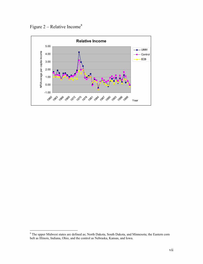
2000a, b). Further, relative farm income (Figure 2) has decreased at an average rate of 4

3 A comment by Chuck Conner, Special Assistant to the President for Agricultural Trade and Food Assistance.

10

percent per year over the last decade (ERS, 2000a; BEA, 2001). Nominal crop prices

have been static, if not declining, while the volatility of prices remains high. For

example, the average nominal price of a weighted basket of corn, soybean, and wheat has

declined at an average rate of 1 percent per year over the last 10 years (NASS, 2001),

while price volatility on a year-to-year basis ranges between 10-15 percent (NASS,

2001). Using Illinois crop farmers as an example, every year over the 5 year period

1996-2000, farmers experienced an average loss of $19,300 on corn and soy production

alone (FBFM, 2001). This is equivalent to a 1.5 billion dollar loss for the state, and if

extrapolated, a loss of $ 4.7 billion each year for the nation. Not only have losses been

incurred over recent years, but they have increasing as well. Over the last 20 years, losses

have risen at an average rate of 8 percent per year.

The ability for crop farmers to sustain these substantial losses is partly attributable

to increasing government support. Over the last 20 years, government payments to the

agricultural industry have increased at an average rate of $520 million per year (ERS,

2001a). In 2000 alone, government payments to the agricultural industry amounted to a

total of $23 billion (ERS, 2001a). Further, the 2002 Farm Bill, at $180 billion, more than

doubles the support to agriculture (Elliott, 2002). The need for these transfers indicates a

fundamental structural problem of fitness at the farm level.

The objective of the empirical analysis is to explore how farmers are responding

to this apparent hostile environment. To analyze farmers’ adaptive practices a cross-

sectional time series representing crop production (corn, soybeans and wheat) in nine US

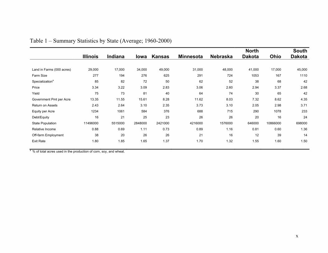
Midwestern states4 from 1963 – 1999 is employed (Table 1). Agriculture being a

competitive industry, allows for relatively high degrees of homogeneity compared to 4 Ohio, Illinois, Indiana, North Dakota, South Dakota, Minnesota Kansas, Nebraska, and Iowa

11

other industries. Technology and information technologies are relatively symmetric

across the industry. This reduces the immeasurable idiosyncratic effects found in

traditional cross-sectional series. In crop production the business form too is relatively

homogeneous being comprised of small corporations underlayed by family ownership

and control. Market prices are exogenous and government payments are allocated by

crop not be region. These features not only allow for less “noise” arising from the data,

but also easier imputation of managerial behavior from industry-level responses. This

research studies five adaptive responses (dependent variables); increasing scale,

increasing specialization, ex-industry diversification, exit and architectural innovation

(Table 2). Two regression models, munificence and hostility, are built to analyze in

forces affecting strategic choice.

Operational Measures5

Incremental change (short jumping) – Romanelli and Tushman (1994)

operationally define incremental change as small-scale changes of internal power

distributions and market breadth, across a considerable time period. Prahalad (1993)

describes this as addressing the productivity gap; a focus on improving performance

across existing dimensions of the firm. Incremental changes are consistent with low risk,

and reversibility that have little affect on the underlying deep structure of the

organization.

Average rate of change of farm size is the first dependent variable analyzed. It

reflects reinvestment associated with scale economies; “doing what one does better.”

The second incremental strategy modeled is the degree of specialization (the percentage

of farm area used for the production of corn, soy and wheat). This reflects a strategy of 5 Summary statistics shown in Table 4.

12

not only increasing efficiency through focus, but also is reflective of environmental risk.

In crop production, diversification is a strategy to manage risk. If one crop fails or one

crop’s price falls, the remainder of the cropping portfolio compensate. Specialization

reflects the “absence” of such turbulence.

Ex-industry diversification (cross jumping) – The third adaptive practiced studied

is off-farm employment. Non-farm income is a particularly important source of

household income for most types of US farms (Offutt, 2000). Agriculture Census data

indicates that off-farm employment levels have been increasing at an average rate of

approximately three percent per year over the last 25 years (NASS, 1999). Ex-industry

diversification is measured as the percentage of farmers working more than 200 days off

farm each year. It is hypothesized such a choice is motivated by forces different from

those inducing within-industry incremental change. That is, an increase in non-business

diversification could be as motivated by a pulling from the macro level of the

environment, as a direct push from low munificence at the resource, sub-environment or

task levels.

Radical Adaptation (long jumping)- Such adaptive strategies typically require a

major reorganization of resources within the firm. This may involve leveraging core

competencies and outside resources or simply de-assetation and exit from the industry.

Industry exit reflects environmental selection against the firm as described by Hannan &

Freeman, (1977) and Aldrich & Pfeffer, (1976). In terms of complexity theory, this

selection is equivalent to the system ‘dying’ after ineffective adaptation at the point of

bifurcation: failure to correct for the fundamental mismatch of organizational form and

environmental context (Prigogine & Stengers, 1984; MacIntosh & MacLean, 1999). It is

13

hypothesised that exit will increase with a pulling force from the macro and aggregate

environment and decrease with the supportive nature of task, sub, and resource

environments. The measure of exit (following Anderson & Tushmans’ (2001)

identification of exit as the termination of production and withdrawal from the industry)

is derived from statistics tracking the decline in the number of farms within any one state

(ERS, 1996).

Alternatively a long jump may entail architectural innovation, similar to

Prahalad’s (1993) opportunity gap approach. In agriculture the adoption of relationship

management (one-to-one marketing) orientation by commodity firms, or the

establishment of ‘long-jump producer-owned ventures,’ such as new generation

cooperatives (NGC’s6) have been identified as a form of long jumping (Goldsmith and

Gow, 2001). NGC establishment involves a large investment of resources, commitments

that are not necessarily reversible, and the acquisition of competencies that are not

necessarily within the existing set of competencies of the producer. As investments of

this type are irrecoverable (irreversible), irrespective of the performance of the venture,

they can be likened to the complexity concept of entropy where firms import new

“energy” and ideas as firms approach bifurcation. The ‘new ideas’, ‘new products’, and

‘new markets’ discussed by Cobia (1997) in relation to NGC’s correspond to Prahalad’s

(1993) ‘imaginative configurations’ and requirement for a stretch of aspiration, and

acquisition of new competencies. Data about NGC formation in the US since 1970 are

6 New generation cooperatives are a relatively modern organizational form, unique to the US. These cooperatives are generally small (<200 producers), closed (meaning not everyone can be a member), require significant equity participation (for capitalizing the firm), commitment in terms of delivery obligations, not purely democratic, involve some form of integrative step (horizontal or vertical), and many times are formed as limited liability companies.

14

used as a proxy for agricultural radical innovation and originate from a data set compiled

by Merritt et al (1999) and Merritt (2002).

Explanatory Variables7

Hostility – Previous theory measures hostility in terms of unexpected

environmental changes and shocks (Covin & Slevin 1989; McArthur & Nystrom, 1991).

In many respects, the operational measures adopted here are not unlike measures of

concepts such as dynamism, malevolence, threat, turbulence, and instability used in

previous studies. In a practical sense, the operational measures adopted here are similar

to Dess and Beard’s (1984) measures of dynamism (stability-instability, turbulence) that

account for variability in the environment, and uncertainty of this variability. Dess and

Beard (1984) found measures such as the variability of sales, margins, employment, and

value added to be valid means of measuring dynamism. This practice to capture

dynamism has since been followed by subsequent research (Shafman & Dean, 1991;

Rasheed & Prescott, 1992; Goll & Rasheed, 1997).

The average change over two year periodsi is used to study hostility’s impact on

organizational adaptation. The lagged measures capture the degree of short term

turbulence of the environment. The independent variables are price, yield, net farm

income, return on assets, and government payments (Table 3). Yield change represents

the general ‘hostility’ of the physical environment (the resource pool level) and captures

7 Summary statistics shown in Table 6.

15

the affects of weather patterns, weeds, pests, plant diseases, and other physical,

biological, and climatic factors effecting the quantity and quality of production.

Net farm income, and return on assets are two firm-level measures that reflect the

current favorability (or hostility) of the sub environment. The two measures are valuable

to account for costs of production; increases being reflective of sub- environmental

hostility.

Crop prices (after appropriately weightingii) are widely reported, thus highly

visible, reflect the task environment in terms of the economic climate and market

conditions. Also, consistent with Aldrich and Pfeffer (1976), temporal declines in

government support are indicative of hostility. Government support has become a large

and influential part of the environment itself in that payments to farmers have been

capitalized into land prices on the basis that they positively contribute to expectations of

future earnings (ERS, 2001). Any short term decline in the level of this support is thus

perceived as an increase in the adversity of the aggregate environment.

Munificence – Previous studies of environmental munificence have generally

empiricized munificence in terms of growth in sales (Yasai-Ardekani, 1989; McArthur &

Nystrom, 1991). More comprehensive investigations of munificence used a variety of

measures including; number of employees, value of shipments, firm concentration ration,

and average market share (Dess & Beard, 1984; Shafman & Dean, 1991). The

munificence model used in this study attempts to reflect the ‘state’ of the environment in

terms of resource abundance or scarcity rather than indirect measures such as “rates of

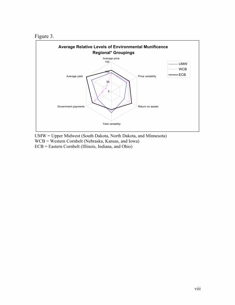
growth.” These measures, made in relative terms (see Figure 3), more accurately reflect

the ‘state’ nature of resource availability and the time dependent development of

16

perceptions that condition behavior in response to munificence. Using relative ten year

averages provides the ability to better capture the way in which the farm managers

perceive the state of their resources base (Figure 4). This differentiates the measurement

of munificence from that of hostility and previous research.

The most basic level of resources are captured by two variables: quality of the soil

and weather, reflected in long term yield differences; and firm wealth, reflected in long

term equity levels. High quality soils or elevated equity levels as resource pools

potentially provide opportunity for a wider variety of adaptive strategies.

Long term trends in return on assets are used to reflect the sub-environment

associated with firms themselves and their control of the resource pool. Higher prices,

like demand growth as measured by Des & Beard (1984) and Shafman & Dean (1991),

are a significant resource in the regional (task) environment. Castrogiovanni (1991)

points to task resources as those affecting the firm and those firms with which it must

interact.

The aggregate level is a higher order still reflecting resources available to not only

the firms but the stakeholder community as well. Government payments, as noted above,

have considerable effects on the expectations of crop producers and as such significantly

influence the decision-making process. Consistent with the aggregate level, these

resources are not entirely dedicated. They can not only reduced but more importantly

redirected to other sectors and missions of the USDA, i.e. nutrition, conservation, and

food safety.

Relative income and munificence of the ex-industry environment reflect the

attraction/repulsion force of the greater macro environment. Relative income is the ratio

17

of average net farm income per farm to average per capita income for the state. An

adaptive response to low relative income would move resources to higher valued

opportunities. Ceteris paribus, under conditions of low relative income a farm-firm

would be expected to reduce investment in agriculture and either increase investment

outside of agriculture or even exit.

Outside opportunities to redeploy capital may be limited at the same time relative

income is low. The ex-industry macro environment is proxied by the number of

metropolitan areas of population greater than 100,000 multiplied by the total number of

people residing in those areas divided by the crop acres in the state. The variable serves

as a proxy for the pool of off-farm or exit opportunities available to farm managers. At

the same time, a high level of industrial activity associated with a significant metropolitan

presence in the state could serve as valuable resource for farm businesses seeking to

shorten the supply chain and serve end-users more directly through new generation

cooperatives.

Results

Final presentation of results was not ready at the time of publication of this version.

Results and discussion and an updated manuscript will be provided at the seminar.

Appendices 1 and 2, which are attached, show the regression results.

i

References AgNews. (1999). “Farmers Under Considerable Stress, Study Shows.” AgNews, News

and Public Affairs, March 17, 1999. Aldrich, H., and J. Pfeffer. (1976). “Environments of Organizations.” Annual Review of

Sociology. 2:79-105. Anderson, P., and M. Tushman. (2001). “Organizational Environments and Industry Exit:

The Effects of Uncertainty, Munificence, and Complexity.” Industrial and Corporate Change. 10, 3:675-711.

Bureau of Economic Analysis. (2001). “State and Local Area Data, Gross State Product

Estimates.” Retrieved 10 January 2001 from the World Wide Web: http://www.bea.doc.gov/ .

Blake, D. (1996). Efficiency, Risk Aversion and Portfolio Insurance: An Analysis of

Financial Asset Portfolios Held by Investors in the United Kingdom.” The Economic Journal. Vol. 106. September. 1175-1192.

Brown, S.L. and K.M. Eisenhardt. (1997). “The Art of Continuous Change: Linking

Complexity Theory and Time-Paced Evolution in Relentlessly Shifting Organizations. “ Administrative Science Quarterly. V.42 N1. March: 1-34.

Carroll, G. R. (1988). "Organizational Ecology in Theoretical Perspective." Ecological

Models of Organizations. G. R. Carroll ed. 1-31. Castrogiovanni, G. (1991). “Environmental Munificence: A Theoretical Assessment.”

Academy of Management Review. 16, 3:542-565. Cobia, D. (1997). “New Generation Cooperatives: External Environment and Investor

Characteristics.” Presentation for the 1997 Food and Agricultural Marketing Consortium Conference, Las Vegas, NV, January 16-17.

Covin, J., and D. Slevin, (1989). “Strategic Management of Small Firms in Hostile and

Benign Environments.” Strategic Management Journal. 10:75-87. Cyert, R., and J. March. (1963). A Behavioral Theory of the Firm. Prentice Hall Inc. New

Jersey. Dess, G., and D. Beard. (1984). “Dimensions of Organizational Task Environments.”

Administrative Science Quarterly. 29:2-73. Economic Research Service. (1996). “Are Farm Bankruptcies a Good Indicator of Rural

Financial Stress?” Agriculture Information Bulletin. No. 724-06, December.

ii

Economic Research Service. (2000a). “U.S. and State Farm Income Data.” Selected states/selected years. Retrieved 10 January 2001 from the World Wide Web: http://www.ers.usda.gov/Data/FarmIncome/finfidmu.htm .

Economic Research Service. (2000b). “Farm Business Balance Sheet and Financial

Ratios.” Selected states/selected years. Retrieved 10 January 2001 from the World Wide Web: http://www.ers.usda.gov/Data/FarmBalanceSheet/fbsdmu.htm .

Economic Research Service. (2001). “Government Payments to Farmers Contribute to

Rising Land Values.” Agricultural Outlook. June-July, 22-26. Elliott, I. (2002). “U.S. trading partners want more farm bill details.” Feedstuffs. Vol. 74

Issue 29. July 15. FBFM. (2001). Farm Income and Production Costs for 2000. Illinois Farm Business

Farm Management Association, Urbana, Illinois. April 2001. Fredrickson, J.W. and A.L. Iaquinto. (1989). “Inertia and Creeping Rationality in

Strategic Decision Processes. Academy of Management Journal. Vol. 32 N. 3. 516-542.

Goldsmith, P. D. and H. R. Gow. (2001). “Strategic Positioning Under Agricultural

Structural Change: A Critique of Long Jump Co-operative Ventures.” International Food and Agribusiness Management Review. Under Review. January, 2002.

Goll, I., and M. Rasheed. (1997). “Rational Decision-Making and Firm Performance: The

Moderating Role of the Environment.” Strategic Management Journal. 18(7):583-591.

Hannan, M. and J. Freeman. (1977). “The Population Ecology of Firms.” American

Journal of Sociology. 82(5):929-964. Khandwalla, P. 1973. “Environment and Its Impact on the Organization.” 297-313. Lagmeyer, J. (2002). Population Statistics 1999/2002. "Populstat" site: Jan Lahmeyer.

Retrieved 10 March 2002 from the World Wide Web: http://www.library.uu.nl/wesp/populstat/Americas/usat.htm .

Lawrence, P.R. and L.W. Lorch. 1967. Organization and Environment; Managing

Differentiation and Integration. Cambridge, MA: Harvard University Press. Leifer, R. (1989). “Understanding Organizational Transformation Using a Dissipative

Structure Model.” Human Relations. 42(10):899-916.

iii

Levinthal, D. (1997). “Adaptation on Rugged Landscapes.” Management Science. 43:934-950.

Levy, D. (1994). “Chaos Theory and Strategy: Theory, Application, and Managerial

Implications.” Strategic Management Journal. 15:167-178. MacIntosh, R. and D. MacLean. (1999). “Conditioned Emergence: A Dissipative

Structures Approach to Transformation.” Strategic Management Journal. 20:297-316.

McArthur, A. and P. Nystrom. (1991). “Environmental Dynamism, Complexity, and

Munificence as Moderators of Strategy-Performance Relationships.” Journal of Business Research. 23:49-361.

McKelvey, B. (1999). “Avoiding Complexity Catastrophy in Coevolutionary Pockets:

Strategies for Rugged Landscapes.” Organization Science. 10(3):294-321. Merrett, C., M. Holmes, and J. Waner. (1999) “Directory of New Generation

Cooperatives.” Illinois Institute for Rural Affairs. Western Illinois University. Merrett, C. (2002). Updated data of New Generation Cooperatives. Unpublished. Illinois

Institute for Rural Affairs. Western Illinois University. Mintzberg, H. (1979). The Structuring of Organizations. Prentice-Hall, Inc., Englewood

Cliffs, N.J. National Agricultural Statistic Service. (1999). 1997 Census of Agriculture. Retrieved 10

January 2001 from the World Wide Web: http://www.nass.usda.gov:81/ipedb/ . National Agricultural Statistics Service. (2001). Agricultural Statistics Series, 1950-2000.

Retrieved 10 January 2002 from the World Wide Web: http://www.usda.gov/nass/ .

Ng, D. and P. D. Goldsmith. (1998). “Micro Economic Evolution of an Organization: A

Dynamic Programming Model of Organizational Evolution.” Annual Meeting of the Canadian Agricultural Economics Association. Vancouver. July.

Offutt, S. (2000). “Can the Farm Problem be Solved?” Economic Research Service, U.S.

Department of Agriculture. ME John Lecture, The Pennsylvania State University, October.

Prahalad, C. (1993). “The Role of Core Competencies in the Corporation.”

Research/Technology Management. November-December:40-47. Prigogine, I. and I. Stengers. (1984) Order Out of Chaos. Bantam. Toronto.

iv

Rasheed, A., and J. Prescott. (1992). “Towards an Objective Classification Scheme for Organizational Task Environments.” British Journal of Management. 3:197-206.

Romanelli, E. and M. Tushman. (1994). “Organizational Transformation as Punctuated

Equilibrium: An Empirical Test.” Academy of Management Journal. 37(5):1141-1168.

Rosenzweig, M.R. and H.P. Binswanger. (1993). “Wealth, Weather Risk and the

Composition and Profitability of Agricultural Investments.” The Economic Journal. Vol. 103. January: 56-78.

Schumpeter, J. A. (1934). The Theory of Economic Development. 5th Edition (1997).

Transaction Publishers. New Brunswick, New Jersey and London, England. Shafman, M., and J. Dean. (1991). “Conceptualizing and Measuring the Organizational

Environment: A Multidimensional Approach.” Journal of Management, 17(4):681-700.

Stacey R. (1995). “The Science of Complexity: An Alternative Perspective for Strategic

Change Processes.” Strategic Management Journal. 16:477-495. Staw, B., and E. Szwajkowski. (1975). “The Scarcity-Munificence Component of

Organizational Environments and the Commission of Illegal Acts.” Administrative Science Quarterly, 20:345-354.

Successful Farming. (1999). Doom and Gloom, Ideas from Washington. 22 February,

1999. Tushman. M., and E. Romanelli. (1985). “Organizational Evolution: A Metamorphism

Model of Convergence and Reorientation.” In Research in Organizational Behavior. L. Cummings, and B. Straw (Eds). Greenwich, CT: JAI Press. 7:171-222.

U.S. Census Bureau. (1990). Decennial Census 1990, Geographic Comparison Tables,

Retrieved January 10, 2001, from the World Wide Web: http://factfinder.census.gov/servlet/BasicFactsServlet on 10-01-02 .

Washington Post, (2002). “Bush Signs Bill Providing Big Farm Subsidy Increases.”

Washington Post. 14 May. Yasai-Ardekani, M. (1989). “Effects of Environmental Scarcity and Munificence on the

Relationship of Context to Organizational Structure.” Academy of Management Journal. 32 (1): 131-156.

v

Zammuto. R. F. (1988). "Organizational Adaptation: Some Implications of Organizational Ecology for Strategic Choice." Journal of Management Studies 25(2): 105-120.

vi

Figure 1. Castrogiovanni (1991) Taxonomy

Macro Environment

Aggregate Environment

Task Environment

Sub-Environment

Resource Pool

vii

Figure 2 – Relative Income8

Relative Income

-1.00

0.00

1.00

2.00

3.00

4.00

5.00

1960

1963

1966

1969

1972

1975

1978

1981

1984

1987

1990

1993

1996

1999

Year

NFI/A

vera

ge p

er c

apita

inco

me UMW

Control

ECB

8 The upper Midwest states are defined as; North Dakota, South Dakota, and Minnesota; the Eastern corn belt as Illinois, Indiana, Ohio, and the control as Nebraska, Kansas, and Iowa.

viii

Figure 3.

Average Relative Levels of Environmental Munificence Regional* Groupings

0

50

100

150Average price

Price variability

Return on assets

Yield variability

Government payments

Average yield

UMW WCB ECB

UMW = Upper Midwest (South Dakota, North Dakota, and Minnesota) WCB = Western Cornbelt (Nebraska, Kansas, and Iowa) ECB = Eastern Cornbelt (Illinois, Indiana, and Ohio)

ix

Figure 4. Conceptual Framework

H Hostility

Hostility Munificence

Macro Environment

Aggregate Environment

Resource Pool

Sub-Environment

Task Environment

Yield

Price

Gov.

Yield/Wealth

Gov.

Price

Metro/Rel. Inc.

ROA ROA

x

Table 1 – Summary Statistics by State (Average; 1960-2000)

Illinois Indiana Iowa Kansas Minnesota NebraskaNorth

Dakota OhioSouth

Dakota Land in Farms (000 acres) 29,000 17,000 34,000 49,000 31,000 48,000 41,000 17,000 45,000

Farm Size 277 194 276 625 291 724 1053 167 1110

Specializationa 85 82 72 50 62 52 38 68 42

Price 3.34 3.22 3.09 2.83 3.06 2.60 2.94 3.37 2.68

Yield 75 73 81 40 64 74 30 65 42

Government Pmt per Acre 13.35 11.55 15.61 8.28 11.62 8.03 7.32 8.62 4.35

Return on Assets 2.43 2.64 3.10 2.35 3.73 3.10 2.05 2.98 3.71

Equity per Acre 1234 1061 584 376 688 715 290 1078 233

Debt/Equity 16 21 25 23 26 26 20 16 24

State Population 11496000 5515000 2848000 2421000 4216000 1576000 646000 10866000 698000

Relative Income 0.88 0.69 1.11 0.73 0.89 1.16 0.81 0.60 1.36

Off-farm Employment 38 20 26 26 21 16 12 39 14

Exit Rate 1.80 1.85 1.65 1.37 1.70 1.32 1.55 1.60 1.50

a % of total acres used in the production of corn, soy, and wheat.

xi

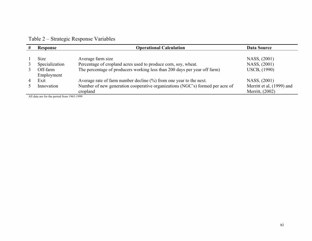
Table 2 – Strategic Response Variables # Response Operational Calculation Data Source 1 Size Average farm size NASS, (2001) 3 Specialization Percentage of cropland acres used to produce corn, soy, wheat. NASS, (2001) 3 Off-farm

Employment The percentage of producers working less than 200 days per year off farm) USCB, (1990)

4 Exit Average rate of farm number decline (%) from one year to the next. NASS, (2001) 5 Innovation Number of new generation cooperative organizations (NGC’s) formed per acre of

cropland Merritt et al, (1999) and Merritt, (2002)

All data are for the period from 1963-1999

xii

Table 3 – Explanatory Variablesa (all models) No. Characteristic Operational Calculation Data Source 1 Price Average weighted price/bushel of a basket corn/soy/wheat NASS, (2001) 2 Price Volatility Longitudinal standard deviation of price for each subject NASS, (2001) 3 Soil Quality Average weighted yield (bushels) of a basket of corn, soy, and wheat, per acre of

cropland NASS, (2001)

4 Weather Longitudinal standard deviation of yield for each subject NASS, (2001) 5 Net Farm Income Average farm income (excluding direct government transfers) per acre of farmlandb ERS, (2000a) 6 Return on Assets Net farm income/total value of farm assets ERS, (2000a), ERS,

(2000b) 7 Government Payments Total direct government transfers per acre of total cropland ERS, (2000a), 8 Metropolitan Areas Number of metropolitan areas (of population greater than 100,000) multiplied by the cumulative

population of those metropolitan areas, on a per acre of farmland basis Lagmeyer, (2002), NASS, (2001)

9 Relative Income Net farm income divided by per capita income ERS, (2001a), BEA, (2001)

10 Equity Average equity value per acre of total farmland (net worth/acre) ERS, (2001b), aRelevant munificence measures are expressed in terms of relative averages. Relevant hostility measures are calculated on an average 2-year difference value. b This net farm income measure does not allow for a return to management.

xiii

Table 4 – Summary Statistics for Munificence Variables MUNIFICENCE Std.dev. (1) (2) (3) (4) (5) (6) (7) (8) 1 Price 0.22 2 Price Variability 0.10 -0.86* 3 Yield 15.82 0.37* -0.08 4 Yield Variability 2.54 0.11* -0.27* -0.64* 5

Return on Assets 0.73 0.05

0.00 0.24* -0.02 6 Government Payments 1.81 0.52* -0.30* 0.69* -0.30* 0.08 7 Metropolitan Areas 0.33 0.61* -0.42* 0.32* 0.04 -0.10 0.09 8 Relative Income 0.28 -0.42* 0.23* -0.07 -0.07 0.48* -0.13* -0.63* 9 Equity 236.98 0.69* -0.43* 0.72* -0.46* -0.06 0.49* 0.63* -0.42*

Mean VIF = 5.0 (Maximum VIF = 11.8) Condition Index for model = 7.5 *p<.05 Table 5 – Summary Statistics for Hostility Variablesa Variable Mean Std. Devb. 1 2 3 4 1 Price 0.04 11.64 2 Yield 0.95 6.25 -0.56 3 Net Farm Income -0.08 -155.70 0.08* 0.424 Return on Assets -0.11 5.62 0.23 0.34 0.755 Government 0.81 -10.89 -0.09* -0.17 -0.60 -0.37 a These are mean difference values (i.e. they represent the average annual change over the 36-year period) b This measure of variance has been standardized for the mean value of the variable. Mean VIF = 2.44 (Maximum = 3.4) Condition Index for model = 3.6 *p<.05

xiv

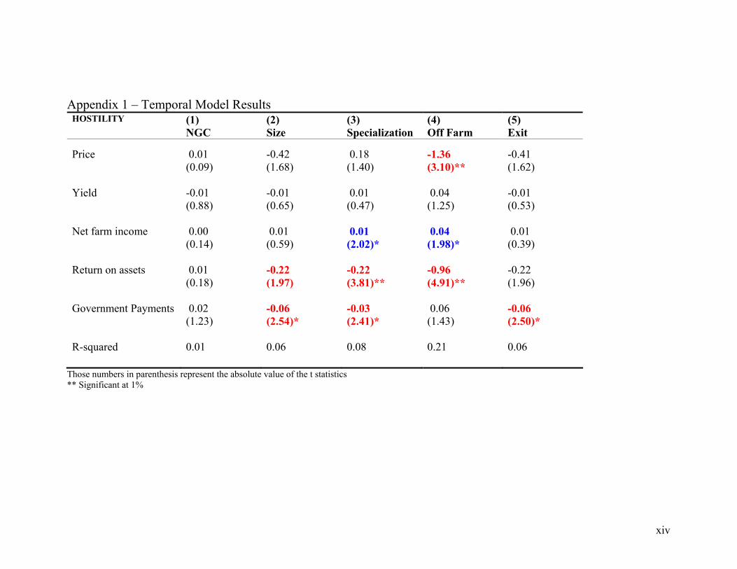
Appendix 1 – Temporal Model Results

HOSTILITY (1) (2) (3) (4) (5) NGC Size Specialization Off Farm Exit Price 0.01 -0.42 0.18 -1.36 -0.41 (0.09) (1.68) (1.40) (3.10)** (1.62) Yield -0.01 -0.01 0.01 0.04 -0.01 (0.88) (0.65) (0.47) (1.25) (0.53) Net farm income 0.00 0.01 0.01 0.04 0.01 (0.14) (0.59) (2.02)* (1.98)* (0.39) Return on assets 0.01 -0.22 -0.22 -0.96 -0.22 (0.18) (1.97) (3.81)** (4.91)** (1.96) Government Payments 0.02 -0.06 -0.03 0.06 -0.06 (1.23) (2.54)* (2.41)* (1.43) (2.50)* R-squared 0.01 0.06 0.08 0.21 0.06

Those numbers in parenthesis represent the absolute value of the t statistics ** Significant at 1%

xv

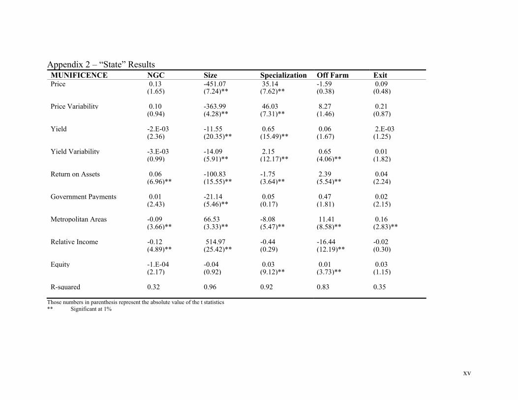
Appendix 2 – “State” Results MUNIFICENCE NGC Size Specialization Off Farm Exit Price 0.13 -451.07 35.14 -1.59 0.09 (1.65) (7.24)** (7.62)** (0.38) (0.48) Price Variability 0.10 -363.99 46.03 8.27 0.21 (0.94) (4.28)** (7.31)** (1.46) (0.87) Yield -2.E-03 -11.55 0.65 0.06 2.E-03 (2.36) (20.35)** (15.49)** (1.67) (1.25) Yield Variability -3.E-03 -14.09 2.15 0.65 0.01 (0.99) (5.91)** (12.17)** (4.06)** (1.82) Return on Assets 0.06 -100.83 -1.75 2.39 0.04 (6.96)** (15.55)** (3.64)** (5.54)** (2.24) Government Payments 0.01 -21.14 0.05 0.47 0.02 (2.43) (5.46)** (0.17) (1.81) (2.15) Metropolitan Areas -0.09 66.53 -8.08 11.41 0.16 (3.66)** (3.33)** (5.47)** (8.58)** (2.83)** Relative Income -0.12 514.97 -0.44 -16.44 -0.02 (4.89)** (25.42)** (0.29) (12.19)** (0.30) Equity -1.E-04 -0.04 0.03 0.01 0.03 (2.17) (0.92) (9.12)** (3.73)** (1.15) R-squared 0.32 0.96 0.92 0.83 0.35

Those numbers in parenthesis represent the absolute value of the t statistics ** Significant at 1%

xvi

Endnotes i The two-year lagged period is adopted only after having first found that the one and three year lagged periods were less desirable predictors of strategic response (that is, after having modeled them against the dependent variables). Also, the measures are deliberately not detrended on the basis that the holistic impact of both variability and trend (cumulative for the various response variables) is an important component of the model as determinants of strategic change. Had the study focused on a more micro-analysis of organizational adaptation (e.g. one specific strategic response), then detrending would be an appropriate if not necessary part of the analytical process. Future research efforts may attempt to distinguish between the specific influence of the trend and the year to year variability. Though it is recognized that both affect strategic response, for the sake of comprehensiveness and parsimony, the effects are not separately analyzed in this investigation. ii Yield is weighted for the proportion of crop type grown. Careful consideration was given to the weighting scheme used (alternatives included weighting relative to the average yield for the population, and no weighting at all). It was found that there is little variation between these indexes (analysis of pair-wise correlation coefficients showed that all relationships were significant at the 0.0001 level), such that potential effects (of differing alternative weighting schemes) on model results are minimal. Thus, a weighting scheme by crop area was selected for its ability to more accurately reflect changes observed at the farm level. This was made on the assumption that firstly, deviation of percentage yield variability across the three major crops is minimal, and secondly farmers are more perceptive to the variability in their own yields than they are to those of neighboring farms, or state or population averages. The same rationale is made for the weighting of price. Again it was found that alternative schemes produce indexes of very high covariance and thus have minimal effect on regression results (this is likely attributable to the high degree of competition both within and between markets for crop products and the relatively high degree of substitutability of crop products (especially in feed markets) in the case of price, and similar effects of rainfall, sunshine hours etc. on all crop types produced in relation to yields). The degree to which risk is endogenized or exogenized by this means of indexing yield and price for the three crop products is an interesting topic for further research.