the externality of driving luxury cars - · pdf file2 the externality of driving luxury cars...
TRANSCRIPT

1
The Externality of Driving Luxury Cars
Sojung Carol Park1
Associate Professor of Finance
College of Business Administration
Seoul National University
1 Gwanak-ro, Gwanak-gu,
Seoul, 151-916, Korea
Email: [email protected]
Phone: +82-02-880-8085
and
Sangeun Han
College of Business Administration
Seoul National University
1 Gwanak-ro, Gwanak-gu,
Seoul, 151-916, Korea
Email: [email protected]
Phone: +82-02-880-8085
This Draft: 2015-01-23
1 Corresponding author
2
The Externality of Driving Luxury Cars
Abstract
Due to a striking difference in repair cost between foreign and domestic car in Korea, the
foreign car drivers increased the property damage liability insurance costs of domestic car
drivers. That is, driving foreign car creates negative externalities. We estimate auto accident
externalities of driving luxury cars (more specifically foreign cars) by running a two part
model (TPM) using individual level panel data on insurance claims and insured’s
characteristics. We find that negative externalities do exist in all of our specifications. To be
specific, a 1% increase in foreign cars raises the property damage liability cost by 3-5.5%
which indicates externality in severity. Each foreign car driver increases the property damage
cost by USD 37-78 per year on average, depending on the specification. The nationwide
increased liability cost is USD 27-48 million per year In Korea, this cost is currently shared
by all drivers including the majority of domestic car drivers.
Key Words: Negative Externalities; Luxury Car; Auto Accidents; Tort Liability
1. Introduction
Two vehicles get into an accident. Under the tort system, the at-fault driver pays for the losses
of both cars. Where a comparative negligence is applicable, the degree of negligence
contributed to the accident is determined and each driver pays for their portion of losses. This
comparative negligence tort system is adapted in many countries including Korea. This
comparative negligence is considered to be quite fair and has been well accepted adjusting
auto accident losses until recent. However, the increasing number of luxury cars generates a

3
debate questioning the fairness of the system.
If the repairing costs of two cars involved in an accident are fairly similar, the
comparative negligence works well. However, when the values of properties vary
significantly, this may not be the case. Consider an accident between an expensive and cheap
car. Let’s assume that the driver of the luxury car was 90% at-fault and the driver of the cheap
car was only 10% at-fault for not doing excellent defensive driving. Both cars had minor
scratches but the repair costs resulted to be $5,000 and $100 respectively. Now the driver of
the luxurious car must pay $90 to his counterparty, and the driver of the cheap car needs to
pay $500. If the repair cost of the luxury car had equaled that of the cheap car that is, $100,
the driver of the cheap car would have only needed to pay $10. Suppose that all of a sudden
your vicinity becomes full of luxury cars. The drivers of cheap cars do not really do anything
bad but the liability costs of the cheap car driver increases as a result of increased luxury cars
around. However, one’s personal preference for luxury cars does not involve an increase in
liability cost for others. The aforementioned example illustrates a negative externality from
driving luxury cars which the tort system is not designed to address.
Repairing costs of cars vary to some extent but this seems to be a universal
phenomenon observed in most countries. However, the price discrepancy becomes a problem
in countries like Korea and China where the repair costs between domestic and foreign cars
differ exceedingly. For example, in Korea, the repair cost of foreign cars is more than five
times higher on average than that of domestic cars of similar size.2 This striking difference is
mostly caused by the costs of expensive parts of foreign cars. The abnormal gap between
foreign and domestic cars is a dramatic issue in China. According to Chinese government, the
2Table A1 and A2 in Appendix shows the repairing cost difference of domestic and foreign cars
and the repairing cost of domestic cars by car type.

4
sum value of individual parts is 12 times more expensive than the price of the car itself. In
August 2014, Chinese authorities fined Volkswagen and Chrysler according to the anti-trust
law for imposing higher prices in China for both vehicles and replacement parts. The
exorbitant costs for spare car parts in Korea and China compared to other countries, lies in
the fact that many automakers in these two countries insist replacement parts to be sold only
through authorized dealers. This kind of monopolistic behavior raises the price of repairing
costs of foreign automakers. Of course, it is not only the repairing cost that differs. Excessive
rental and vehicle prices of foreign luxury cars also burdens drivers and insurers.
As a result, the insurance premiums of foreign cars are more expensive than that of
domestic cars. Korean Insurance Development Institution recently announced that own car
property damage coverage rate will be adjusted in 2015 and this will increase the rate of
foreign cars by 11% on average. Some may consider that the increase in coverage solves the
externality problem. However, it does not address the negative externality issue of foreign
cars because the raise only applies to the property damage of own cars.
Along with the dramatic speed of economic development, the size of automobile
market in Korea also grew very fast during the last few decades. Number of cars increased
from 53,000 in 1980 to 1,940,000 in 2013, which is a 3,660% increase in 30 years. The
Korean automobile market was dominated by domestic cars for a long time. However,
recently, due to the rapid increase in income and active market opening, the number of
foreign cars has been grown rapidly. The number of foreign cars quintupled in eight years;
the number of registered foreign cars was 138,000 (1.25% of all registered car) in 2005 and
this increased to 724,000 (4.8% of registered car) in 2013. In some districts in Seoul, the ratio
of registered foreign cars is more than 20%. The growth in foreign car segment in the overall
automobile market is expected to accelerate even further since the FTA with EU and the

5
United States came into effect, granting price competitiveness to foreign cars.
As shortly mentioned above, repairing foreign cars is much more costly than
domestic cars and this may affect the decision of purchasing foreign cars. However, this cost
is not fully borne by the owner of the vehicle but is shared by all other drivers on the road
through the liability costs under the tort system. Therefore, the expensive repair cost may not
fully provide an incentive to hinder the purchase of luxurious cars. This results in increased
liability costs of all other drivers. Such situation arouses controversy since usually wealthy
people tend to purchase foreign cars. That is, personal decisions of affluent people may
burden people with relatively lower income in a circuitous route.
Does this negative externality of driving luxury car really exist in practice? That is,
did the liability cost really increase? It is, in fact, not that obvious. Due to driver’s awareness
of high repair costs of foreign cars, drivers may show defensive driving as an effort to reduce
losses. For example, drivers may try to hold distance from luxury cars on the road or in
parking lots. Such behavior may help foreign cars not to increase accident severity, or may
even reduce accident frequency.
Our paper is not the first research examining the accident externalities of driving.
Vickrey (1968) discussed accident externality from driving. Through examining two groups
of California highways he found out that higher traffic density leads to substantially higher
accident rates. Vickrey’s work was further extended by Edlin and Kraca-Mandic (2006) who
attempted to provide better estimates of the aggregated accident externality from driving.
Huang, Tzeng, and Wang (2013) used individual-level data in Taiwan and showed the
negative externality exists. All of the studies focus on the quantity of driving.
However, there is no work examining the magnitude and the sign of the externality
from driving luxury cars despite of its significance and the controversy it raises. The purpose

6
of this paper is to empirically examine the existence of negative externality of driving luxury
cars and estimate the extent of it. We estimate the relationship between the foreign car ratio
and the accident frequency and severity using two part model.
The liability cost is measured by insurer costs in this study. Figure 1 shows the
positive relationship between insurer costs of property damage liability per accident (claim
severity) and the foreign car ratio of a given region in 2013. This positive correlation
indicates possibly existing negative externality from driving luxury cars.
[ FIGURE 1 ABOUT HERE]
Difference in foreign car ratio is not the only possible explanation for the relationship
shown in Figure 1. In order to address alternative reasons such as differences in car types,
road conditions, and demographics, we run multivariate regressions with panel data from
2009-2013 controlling for region and year fixed effect, and individual level variables that are
known to affect accident frequency and severity. We also include density, following previous
researches on driving externality.
We find that negative externalities do exist. The claim severity of property damage
liability increases significantly, as foreign car ratio increases whereas accident frequency
stays unaffected. As severity increases and frequency is not affected, the total effect of
foreign car on liability loss is positive. In Seoul, which has the highest ratio of foreign cars,
we estimate that foreign cars increase auto liability costs by 3,798 won (appx. USD 3.8) to
6,694 won (appx. USD 6.7) per driver per year depending on the specification. This
corresponds to a total annual increase of 11,474,627,742 won (appx. USD 11 million) to
20,224,106,926 won (appx. USD 20 million) in loss. The total increase in costs nationwide

7
reaches over USD 27-48 million. Our conclusion is robust to all specifications.
In the next part we suggest the framework for luxury car accident externality. The
data are presented in section 3. Section 4 presents the main results of regressions. The
robustness of results is discussed in section 5. Section 6 concludes.
2. The Framework
Let N be the number of total cars on road and let F be the number of foreign cars. The ratio of
foreign cars is F/N. When considering a car accident, the probability of encountering a
foreign car will be F/N the expected liability cost of a given driver i can be illustrated as
follows:
c = c1 ×N−F
N+ c2 ×
F
N= c1 + (c1 − c2) ×
F
N= α1 + α2 ×
F
N (1)
where c1 represents the average liability when the other car is domestic car and c2 is the
average liability when your other party drives a foreign car. (c1-c2) is the increased cost due to
the foreign car on roads. We expect the cost of property damage liability per accident to be
strictly positive for α2. The effect on accident frequency is however, uncertain. If high costs
of repairing foreign car encourages drivers to drive more cautiously, accident frequency and
foreign car ratio may have negative relationship. The combined effect of all of these on total
liability cost is, therefore, ambiguous.
3. Data
Our data was obtained from one of the largest insurance companies in Korea. The individual-

8
level insurance data contains auto insurance claim records, coverage choice, premium, and
rating factors. Rating factors includes variables such as policyholder’s age, gender, car age,
type of car, capacity, and registered. The claim records can be used as a proxy for accident
information including accident frequency and severity.
In order to examine the effect of foreign car on liability cost, we obtained foreign car
ratio of 16 administrative regions in Korea from The Ministry of Land, Infrastructure and
Transportation. Table 1 shows the 16 district and the registered foreign car ratio in 2009 and
2013. The cross sectional and time series difference of foreign car ratio during the sample
period is quite significant; in 2013, the foreign car ratio of Seoul area is about 7% and the
foreign car ratio of Gyeongbuk region is only 1.36%. Moreover, during the sample period,
the foreign car ratio increased more than 350% in Daegu area whereas the increase rate only
comes to 10% in Busan area.
[TABLE 1 ABOUT HERE]
Unfortunately, information on foreign car registration is somewhat contaminated by
car registration fee difference across regions. In order to attract more vehicles to be registered
and collect more tax, Gyeongnam province reduced its tax rate significantly in 2008. Since
vehicle registration requires a valid address in the given area, for personally owned cars,
registration region mostly corresponds with the region of residence. However, the policy
leaved loopholes for auto lease firms. Many auto lease firms opened up a little office in
Gyeongnam and registered their cars there. Gyeongnam province even opened up a vehicle
registration office in Gangnam district, Seoul where the foreign car ratio is the highest in
Korea for convenience. Inchoen, which is very close to Seoul, followed Gyeongnam's

9
strategy, they lowered tax rate in 2011. As a result, Gyeongnam, which is not a metro city but
a country area, has very an extremely high foreign car ratio and especially an unusually high
business vehicle ratio as is shown in Table A3 in Appendix II. The foreign car growth rate in
Gyeongnam drops substantially in 2011 when Inchoen lowered the tax rate. From 2012, we
can see that the foreign car growth rate is unusually high and the business vehicle registration
surges in Incheon.
Because of this contamination, we adapt a few strategies to minimize noise created
by this tax issue. First, we discard Gyeongnam data, which we consider to be unsound due to
the aforementioned reasons. Second, we calculate a modified foreign car ratio as follows and
apply the modified ratio in further analyses. We first assume that Gyeongnam's true foreign
car ratio is close to Gyeongbuk, which shares the most similarities in geographical, cultural,
political, and economical aspects. Then, we estimate the number of foreign cars driven in
Seoul but registered in Gyeongnam by subtracting the number of registered foreign cars in
Gyeongbuk from the number of registered foreign cars in Gyeongnam. Then we add back this
number to the number of foreign cars in Seoul. For Inchoen, we assume the foreign car
growth rate is 40% in 2012 and 2013 and estimate the true foreign cars driven in Incheon.
Again, we add back the difference to Seoul for year 2012 and 2013. As a robustness check,
we run regressions with original foreign car ratio without Gyeongnam for whole years and
Inchoen in 2012 and 2013. The results remain the same. Additionally, we run regressions
using Gangnam district dummy variable as an alternative measure for foreign car. The
procedure of Gangnam regression is detailed in section 6 robustness checks.
From year 2009 to year 2013, we obtained 17,597,536 individual level panel
observations. We also delete Sejong which is a small special administrative city at the border
of three other regions because the lack of information during the former years. After the

10
deletion of Sejong and Gyeongnam province, we have 16,124,423 observations. The sample
has 15,324,560 observations after the deletion of missing variables. Only a quarter of the
policies in 2013 data have completed one year information because the termination date of
the other 3/4 were not arrived when we attained the data. Therefore, we discard these
observations when we analyze total loss and claim frequency. After the deletion of part of
2013 observation, we have 14,061,546 observations. For the analysis of per accident severity,
we only analyze the observations with positive liability property damage claims. In this part
we include all data of 2013 year data because per accident severity is not affected by the fact
the accident information does not contain the full year information. The number of
observation of this sample is 1,534,388. Table 2 shows the definitions for all variables used in
the study.
[TABLE 2 ABOUT HERE]
We control for region and year fixed effect in the regression analysis. In addition, we
add density as a control variable as is suggested by Vickrey(1968), Edlin and Kraca-Mandic
(2006), and Huang, Tzeng, and Wang (2013). Density is defined as the yearly average km
driven divided by the average length of lanes in each region following Edlin and Kraca-
Mandic (2006). The average driven km of each district is obtained from the Korean
Transportation Safety Authority and the average length of lanes is from Korean Statistical
Information Service.
[TABLE 3 ABOUT HERE]

11
Summary statistics are presented in Table 3 and 4. Panel A of Table 3 presents summary
statistics of dependent variables and continuous explanatory variables. The probability of
property damage liability claim is about 11% in our sample. The average claim size was
approximately USD 1,000. Figure 2 shows the distribution of claim severity. The distribution
is skewed and is far from normal distribution. For regression analyses, we log-transform the
severity. The log severity is close to the normal distribution as is shown in Figure 3.
Panel B. of Table 3 presents the correlation between continuous variables and
dependent variables. The correlation between foreign car ratio and density is quite high at
0.57. Although we have a very large number of observations, the foreign car ratio and density
variables only vary at the level of region and year. Due to the concern of possible
multicollinearity issue, we run regressions with and without density variable. In this
univariate relationship, the correlations between severity and foreign car ratio and between
frequency and foreign car ratio are positive. The correlation between density and severity is
negative and the correlation between density and frequency is negative. All correlations are
significant at 1% level.
[FIGURE2 ABOUT HERE]
Table 4 provides summary statistics of rating variables. All of the variables in this
table are categorical rating variables. Percentage shows the percentage each category
accounts for. Mean loss is the average loss reflecting both frequency and severity of claims.
Claim probability and claim severity shows the average claim frequency and average per
accident claim amount for each categorical variable. Accident severity and frequency is
lowest for the age group 30 to 40, car age older than 15, small capacity cars, age limit of 35

12
year old or higher, driving experience more than 4 years, couple only coverage option, low
mileage option, no traffic violation group, and higher BMS coefficient group (bonus group).
Gender, foreign car, and sports car show the opposite effect on frequency and
severity. Male drivers tend to have higher accident severity but lower frequency. Male drivers
are possibly more aggressive but skillful at the same time, so they tend to have fewer
accidents but given an accident the severity tends to be higher. Foreign car has a negative
sign in frequency but positive in severity. Foreign car drivers tend to drive more carefully but
once they have an accident, the severity is higher. This also applies to sports cars. A possible
explanation for this is that the total driven mileage of a sports car may be lower in
comparison with others since they are generally used as a second car for leisure purposes. As
a result, sport cars may have lower accident frequency but higher severity.
4. Methodology
4.1. Two-part model
The goal of our paper is to estimate the effect of foreign cars on the liability claims. Because
loss data only have positive numbers when accidents occur and claim is reported, the loss
data has a large proportion of zeros. The liability losses can be considered as having two
separate data generating processes: one for the accident frequency and the other for the
severity if claims. One simple approach for large proportion of zeros is running the well-
known Tobit model with lower censored boundary at zero. Tobit model assumes that there is
a latent variable yi∗ which has the following linear regression model:
yi∗ = Xi
′β + ϵi (2)
13
We observe yi = max(yi∗, lb), where lb is the lower boundary of observations. In our case,
lb corresponds to zero. Tobit regression allows estimating the unbiased marginal effect of X
on the latent variable yi∗ and yi in many cases. This, however, is inappropriate because
Tobit regression assumes that a single latent variable determines both the magnitude of
severity and the frequency of losses, which may not be the case. For example, more skillful
but aggressive male drivers may have lower accident frequency but higher severity given an
accident than female drivers.
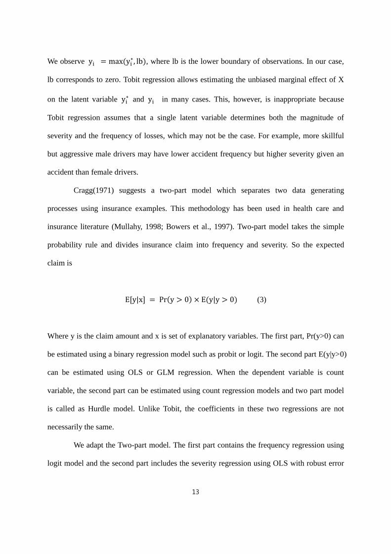
Cragg(1971) suggests a two-part model which separates two data generating
processes using insurance examples. This methodology has been used in health care and
insurance literature (Mullahy, 1998; Bowers et al., 1997). Two-part model takes the simple
probability rule and divides insurance claim into frequency and severity. So the expected
claim is
E[y|x] = Pr(y > 0) × E(y|y > 0) (3)
Where y is the claim amount and x is set of explanatory variables. The first part, Pr(y>0) can
be estimated using a binary regression model such as probit or logit. The second part E(y|y>0)
can be estimated using OLS or GLM regression. When the dependent variable is count
variable, the second part can be estimated using count regression models and two part model
is called as Hurdle model. Unlike Tobit, the coefficients in these two regressions are not
necessarily the same.
We adapt the Two-part model. The first part contains the frequency regression using
logit model and the second part includes the severity regression using OLS with robust error

14
adjustment. The total marginal effect is estimated from the equation (4).
4.2. First part: the effect of density on loss frequency
Our five year panel data includes the number of claims filed by policyholders. We run a logit
regression with dependent variables being zero if there is no claim and one if there is a
claim.3
The model is expressed as following:
Number of claims = Logit(𝛼𝑡 + 𝐹𝑜𝑟𝑒𝑖𝑔𝑛𝑖,𝑡𝛽𝑓 + 𝑋𝑖,𝑡𝛽𝑥 + 𝑍𝑖,𝑡𝛽𝑧)(4)
The βs are the corresponding coefficients and 𝑋𝑖 is the vector of information on each insured,
including characteristics of both the policyholder and the vehicle and 𝑍𝑖 represents the
vector of region information. In order to control fixed effects of year, year dummies are
included. A significant and negative 𝛽𝑓 means that more foreign vehicles in region cause
fewer accidents. Out of concern of multicollinearity, we run regressions with and without
density. In this claim frequency regression, we expect the density variable to have positive
and significant coefficient as is shown in the previous driving externality literature.
4.3. The effect of foreign car ratio on loss severity
In order to examine the externality of driving foreign car on the loss severity we use the OLS
3 As we can observe the number of reported auto insurance claim, we also consider either poisson or negative
binomial regression. Negative binomial regression fits better when modeling over-dispersed count outcome
variables, which is the case of our sample. We additionally run negative binomial regression. The results of
negative binomial regression are almost the same as the one with logit regression. Results are available upon
requests.
15
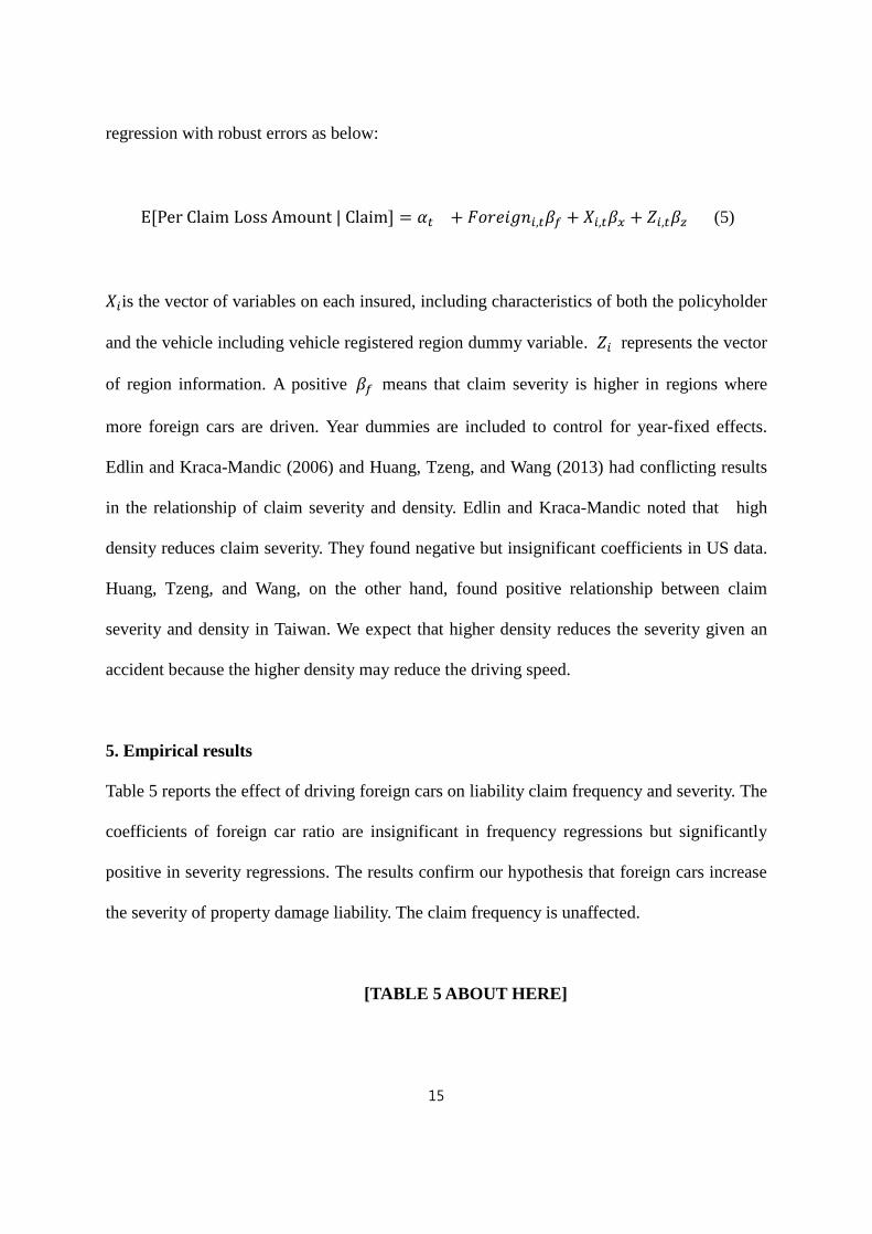
regression with robust errors as below:
E[PerClaim LossAmount|Claim] = 𝛼𝑡 + 𝐹𝑜𝑟𝑒𝑖𝑔𝑛𝑖,𝑡𝛽𝑓 + 𝑋𝑖,𝑡𝛽𝑥 + 𝑍𝑖,𝑡𝛽𝑧 (5)
𝑋𝑖is the vector of variables on each insured, including characteristics of both the policyholder
and the vehicle including vehicle registered region dummy variable. 𝑍𝑖 represents the vector
of region information. A positive 𝛽𝑓 means that claim severity is higher in regions where
more foreign cars are driven. Year dummies are included to control for year-fixed effects.
Edlin and Kraca-Mandic (2006) and Huang, Tzeng, and Wang (2013) had conflicting results
in the relationship of claim severity and density. Edlin and Kraca-Mandic noted that high
density reduces claim severity. They found negative but insignificant coefficients in US data.
Huang, Tzeng, and Wang, on the other hand, found positive relationship between claim
severity and density in Taiwan. We expect that higher density reduces the severity given an
accident because the higher density may reduce the driving speed.
5. Empirical results
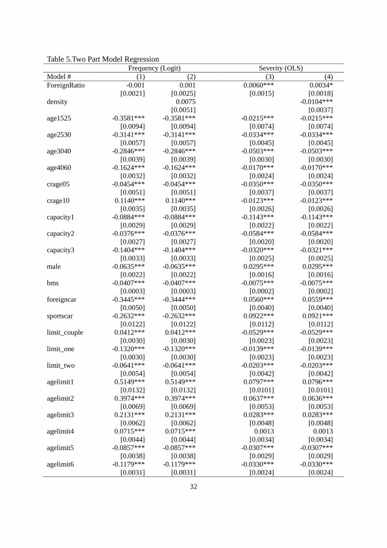
Table 5 reports the effect of driving foreign cars on liability claim frequency and severity. The
coefficients of foreign car ratio are insignificant in frequency regressions but significantly
positive in severity regressions. The results confirm our hypothesis that foreign cars increase
the severity of property damage liability. The claim frequency is unaffected.
[TABLE 5 ABOUT HERE]

16
The results of density are noteworthy. Our frequency results show that density has a
positive but insignificant impact, suggesting possible negative driving externalities as is
found in Edlin and Kraca-Mandic (2006) and Huang, Tzeng, and Wang (2013). However, the
severity is rather lower in areas with high density. This result is consistent with Edlin and
Kraca-Mandic (2006) but opposes the results of Huang, Tzeng, and Wang (2013). Conflicting
results are not so strange, though, because the negative externality of density may vary in
different locations. When the density is too high, higher density may reduce frequency. It is
also possible to have lower severity in high density area if better planned roads are
constructed as demanded, or safer conditioned roads attract more drivers, high density may
yield lower frequency and severity. Therefore, the verification of driving externality is left to
empirical studies.
The results of other control variables are mostly significant and have expected signs.
Most individual characteristic variables have the same sign in both severity and frequency
regression implying that high risk drivers tend to have both more and heavier accidents . A
few variables show the opposite sign as is already shown in the data section. The multivariate
regression results are mostly consistent with the univariate comparison in Table 5. The only
difference is the age variables. This could be due to the fact that the age limit options and age
variables are highly correlated and the age variable shows incremental information after
controlling for the age limit coverage. Among all variables, bonus-malus coefficient had by
far the highest Chi-square in the frequency regression followed by driving experience of one
year. It suggests that there are much of unobserved or unused information in auto insurance
rating, and those are well captured in the bonus malus coefficients. In severity regression,
capacity1 and bonus-malus coefficient had the highest t value.
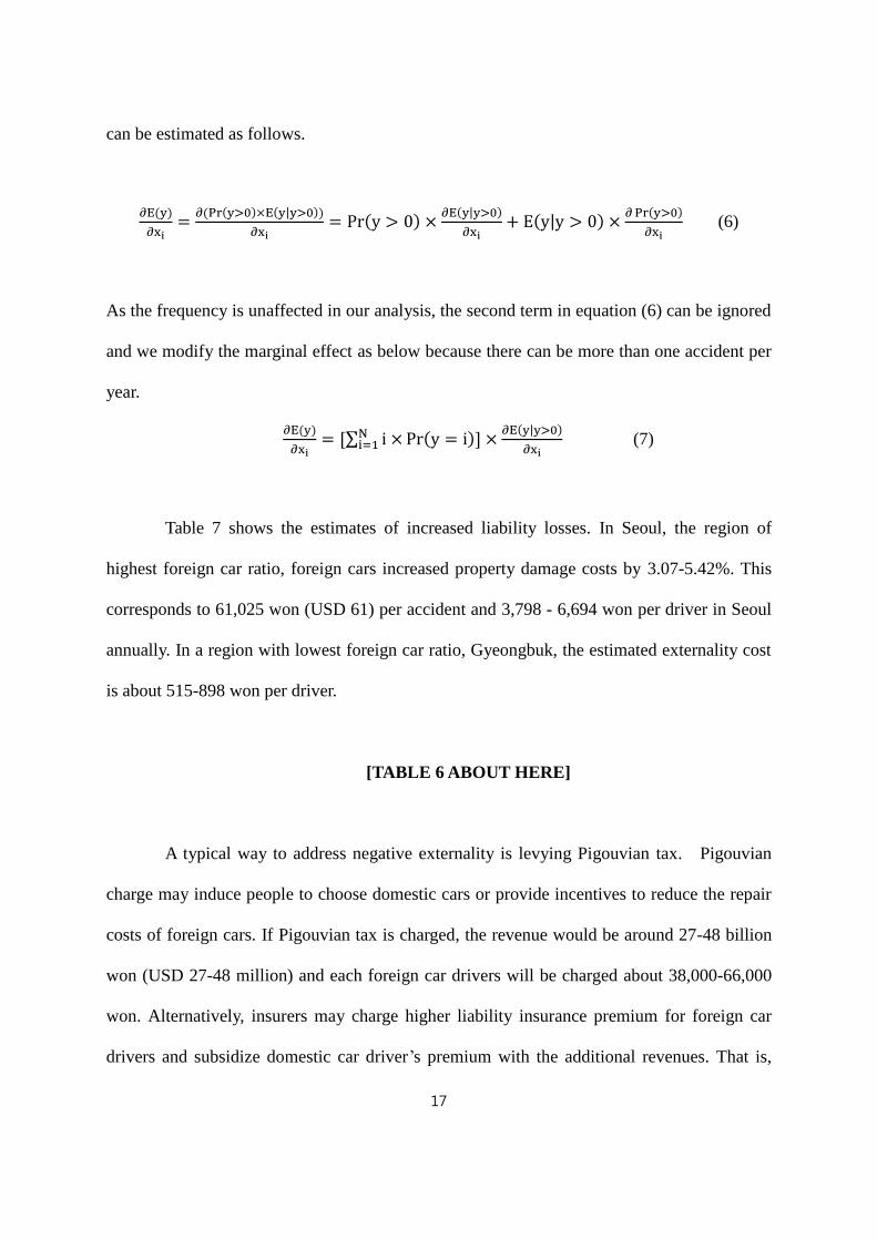
After running two-part model, the marginal effect of a continuous variable xi on y
17
can be estimated as follows.
∂E(y)
∂xi=
∂(Pr(y>0)×E(y|y>0))
∂xi= Pr(y > 0) ×
∂E(y|y>0)
∂xi+ E(y|y > 0) ×
∂Pr(y>0)
∂xi (6)
As the frequency is unaffected in our analysis, the second term in equation (6) can be ignored
and we modify the marginal effect as below because there can be more than one accident per
year.
∂E(y)
∂xi= [∑ i ×N
i=1 Pr(y = i)] ×∂E(y|y>0)
∂xi (7)
Table 7 shows the estimates of increased liability losses. In Seoul, the region of
highest foreign car ratio, foreign cars increased property damage costs by 3.07-5.42%. This
corresponds to 61,025 won (USD 61) per accident and 3,798 - 6,694 won per driver in Seoul
annually. In a region with lowest foreign car ratio, Gyeongbuk, the estimated externality cost
is about 515-898 won per driver.
[TABLE 6 ABOUT HERE]
A typical way to address negative externality is levying Pigouvian tax. Pigouvian
charge may induce people to choose domestic cars or provide incentives to reduce the repair
costs of foreign cars. If Pigouvian tax is charged, the revenue would be around 27-48 billion
won (USD 27-48 million) and each foreign car drivers will be charged about 38,000-66,000
won. Alternatively, insurers may charge higher liability insurance premium for foreign car
drivers and subsidize domestic car driver’s premium with the additional revenues. That is,
18
liability insurance premium can be raised by 38,000-66,000 won (USD 38-66) for foreign car
drivers and domestic car driver’s insurance premium can be cut by 1,400-2,500 (USD 1.4-2.5)
per person annually. This means 21%-37% premium increase for foreign car drivers and
0.8%-1.5% decrease for domestic car drivers.
6. Robustness Checks
6.1. Gangnam district regression
The registered foreign car ratio data is somewhat contaminated because of vehicle
registration tax issue detailed in data section. In order to reduce the noise created by this issue,
we have created a modified foreign car ratio. Out of concern that our modified ratios are still
somewhat inaccurate, we examine the effect of foreign cars in an alternative way.
In Seoul, the capital city of Korea reside about 20% of Korean population in 2014.
Also, the foreign car ratio is the highest in this region. There are 25 districts in Seoul. These
districts are pretty homogeneous compared to other regions in Korea in terms of population
distribution, hospital costs, and etc., but wealth distribution and foreign car ratios within in
Seoul vary quite significantly. Among the 25 two - Gangnam gu and Seocho gu, are theso-
called “Gangnam” area, also being spotlighted in the famous singer Psy's "Gangnam Style". .
Gangnam area can be considered as Seoul's Beverly Hills. Housing prices are notoriously
high and the foreign car ratio is known to be the highest among all districts in Korea.
Due to data restriction, we do not have an access to the foreign car ratios of 25
districts in Seoul. So we instead make a dummy variable for Gangnam. Our strategy is to run
regressions with this dummy variable using observations of Seoul and test whether the per
claim severity is higher in these areas. Figure 3 shows the average foreign car ratio calculated
from our database. The foreign car ratio in Figure 3 might be biased if foreign car owners

19
show preference for the certain insurance company we gained our data from. However, if the
preference is a stable factor and does not differ across time and districts, our estimates in
figure 3 will be relatively plausible.
Because the number of foreign cars increased explosively in this area during the
sample period we also run regressions year by year and examine whether the coefficient of
Gangnam dummy changes or not. We hypothesize that the per claim severity of the property
damage liability is larger in Gangnam area and the difference increases over time. For
frequency, we conjecture that accident frequency is higher in this region as it has higher
density. We expect that the accident frequency difference between Gangnam and non-
Gangnam does not change over time if foreign car ratio does not affect the accident frequency
as is found in the previous section.
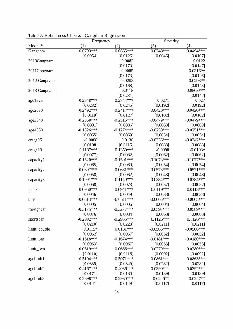
[TABLE 7 ABOUT HERE]
Table 7 presents the result of Gangnam regressions. The results are consistent with
our hypotheses. The property damage severity is higher compared to other districts in Seoul.
As predicted, property damage severity monotonically increases over time in Gangnam area,
supporting the foreign car effect. Frequency is also higher in Gangnam, which reflects the
density effect. Time trend is not found in frequency regression.
6.2. Censored Losses
Since we used claims as a proxy of actual accidents our data is prone to variable truncation
issues. First, very minor accidents may not be observable due to the so-called bonus hunger
behavior. Although we do not have an issue with deductibles because the deductible only

20
applies to the own car's property damage, not the liability losses, some people may not report
small accidents because their auto insurance premium will increase as a result of a claim.
This is less likely to be an issue in Korea because Korea adopts a somewhat unique national
bonus-malus system which reflects the severity of an accident. Korea's bonus-malus system
does not penalize accidents which only involves minor property damages. So it is known that
most of the accidents are reported. Consistent with this, we do observe quite a few
observations with property damage severity below 200,000 won (appx. USD 200); 7 % of
property damage liability losses are below 200,000 won in our sample.
Another possible problem is that the loss exceeds the limit of liability coverage. For
property damage liability, there are ten options to choose from. The coverage choice is shown
in Figure 4. Most drivers chose 100,000,000 won (appx. USD 100,000) as a limit in 2009 and
about 60% opt for a coverage of higher than 200,000,000 won (appx. USD 200,000) in 2013.
This dramatic change is probably due to the foreign car ratio increase. Auto insurance
agencies explicitly mention on their websites “We recommend higher limits due to the
increased number of foreign cars.” In addition, cases of accidents with extra ordinarily
expensive property damage liability costs were publicized through SNS and media,
encouraging people to change their limits.
This, in fact, may bias our results. If the coverage change coincides with foreign car
ratio, which is likely if policyholders behave rationally, and property damage liability losses
are often truncated due to the limit, foreign car ratio and the claimed loss severity may have a
positive relationship even without any actual cost changes due to foreign cars. Out of this
concern, we first examine the possibly censored losses. About 5% of people chose the
mandatory coverage of 10,000,000 won. Among over the 1.5 million property damage
liability losses, in 84 cases the size of loss equaled the limit of property damage and 68 out of
21
84 cases had the lowest limit of 10,000,000 won. So the impact of censored loss seems to be
minor.
To address censored data issue, we conduct regressions excluding those who selected
10,000,000 won limit. This new sample includes 20 censored cases out of over 1.5 million
claims. In addition, we run Tobit regression with an upper limit of 10,000,000 using the full
sample. The results of these two regressions are presented in Table 8. Results remain mostly
unchanged in both specifications.
[TABLE 8 ABOUT HERE]
7. Conclusions
This article examines the externalities of driving luxury cars. We examine the effect of
foreign car ratio on property damage liability claims in a sample of 14,061,546 individual
level panel data between 2009 and 2013 in Korea.
Using the two-part model, we find significant evidence that driving foreign cars
generates negative externality in Korea. We find that foreign cars increase per claim severity
of property damage liability and have insignificant effect on the frequency. The combined
effect increases liability costs of all drivers. Specifically, on average, in Seoul, the region of
highest foreign car ratio, foreign cars increased property damage costs by 3.07%-5.42%. This
corresponds to 61,025 won (USD 61) per accident and 3,798 - 6,694 won per driver in Seoul
annually. This result is robust to numerous specifications such as censored regression and
small sample regression. The same negative externality was found when we run an alternative
regression using Gangnam dummy variable for Seoul sample only.
The results suggest that foreign car owners cause negative externality and this cost is

22
currently shared by the majority of domestic car drivers. As foreign car owners are generally
wealthier than domestic car driver, this is a quite controversial issue in Korea. According to a
project perception survey by KAIDA (Korean Automobile Importers & Distributers
Association) in 2008, 56 percent of people show negative public opinion on foreign car
owners. 24 percent of foreign car owners have a fear of personal harm or loss due to this
negative perception (KAIDA, 2008). Mass media partly aggravates such negative perception
by often publicizing the unfairness of liability losses when having an accident with foreign
cars.
Regulators are aware of this fact and try to resolve the issue. In order to reduce the
increased property damage costs, insurers currently consider offering a similar sized domestic
car as a rental car when foreign car is under repair, using alternative parts instead of the
authentic dealer provided parts in order to lower repair costs, and etc. Some even argue to
move on no-fault system. Considering the current negative perception and the fear of harm
that foreign car owners have, no-fault system does not seems to be a good solution because
this may create large moral hazard issue. Unless Korean government finds a way to reduce
the repair cost disparity between foreign cars and domestic cars to a reasonable level, the
social stress caused by the negative externality will keep increasing.
Our research focuses on the negative externality caused by luxury cars in Korea. This,
however, is not limited in Korea. For example, China faces the same issue. Many other
countries whose domestic car manufacturers compete with foreign brands may have the same
repair cost structure, thus suffer from similar kind of negative externalities. Although the
level of repair cost can be much smaller in other countries, luxury cars on road about
anywhere in the world are just more expensive to repair, causing the same issue. This kind of
negative externality also does not need to be limited to cars. Expensive properties around

23
may increase the liability risk. An expansion and application of this idea can be numerous.
References
Bowers, Newton L., Hans U. Gerber, James C. Hickman, Donald A. Jones and Cecil J.
Nesbitt, 1977, Acturial Mathematics, Society of Actuaries, Schaumburg, IL.
Cragg, John G., 1971, Some statistical models for limited dependent variables with
application to the demand for durable goods, Econometrica 39(5), 829-844.
Edlin, A. S., and P. Karaca-Mandic, 2006, the Accident Externality from Driving, Journal of
Political Economy, 114(5): 931-955.
Huang,R.J, L.Y.Tzeng, and K.C. Wang, 2013, Heterogeneity of the accident externality from
driving, Journal of Risk and Insurance
Korea Automobile insurance repair research and training center, 2011, available at:
http://www.kidi.or.kr/about/about06_view.asp?no=371&Cur_Page=1&s_kw=%BC%F6%B8%AE%B
A%F1&select2=0
Mullahy, John, 1998, Much ado about two: Reconsidering retransformation and the two part
model in health econometrics, Journal Health Economics 17, 247-281.
Parry, I. W. H., M. Walls, and W. Harrington. 2007. Automobile Externalities and Policies,
Journal of Economic Literature, 45(2): 373-399.
Vickrey, W., 1968, Automobile Accidents, Tort Law, Externalities, and Insurance: An
Economist’s Critique, Law and Contemporary Problems 33(summer): 464-487.

24
Figure 1. Foreign car ratio and claim severity
0
2
4
6
8
70 80 90 100 110 120
Fore
ign c
ar
ratio(%
)
Per Claim Severity(10,000 won)
Foreign Car Ratio and Claim Severity in 2013

25
Figure 2. Claim Severity Distribution

26
Figure 3. Foreign car ratio change in Seoul
Figure 4. Change in Liability: Property damage Coverage Distribution (unit: won)
23.4 25.5 25.1
30
34.7
6.7 7.5 7.7 10.2
12.8
16.7 18 17.4
19.8 21.9
0
5
10
15
20
25
30
35
40
2009 2010 2011 2012 2013
Ratio(%
)
Gangnam
Non-Gangnam
Difference
0%
20%
40%
60%
80%
100%
2009 2010 2011 2012 2013
1,000,000,000
500,000,000
300,000,000
200,000,000
100,000,000
70,000,000
50,000,000
30,000,000
20,000,000
10,000,000

27
Table 1. Foreign Car Ratio by State/Year Number of Registered Foreign Cars Percentage of Registered Foreign Cars to
All Registered Cars(unit: %)
2009 2013 % Increase 2009 2013 % Increase
Seoul 120,643 205,676 70.48% 4.08% 6.93% 69.85%
Busan 55,655 64,319 15.57% 4.97% 5.45% 9.66%
Daegu 10,548 54,376 415.51% 1.16% 5.23% 350.86%
Inchon* 9,108 45,229 396.59% 1.01% 3.97% 293.07%
Gwangju 6,675 17,478 161.84% 1.36% 3.07% 125.74%
Daejon 5,713 16,354 186.26% 1.04% 2.68% 157.69%
Ulsan 2,822 7,960 182.07% 0.66% 1.62% 145.45%
Gyeonggi 68,207 157,675 131.17% 1.70% 3.48% 104.71%
Gangwon 3,786 9,960 163.07% 0.64% 1.53% 139.06%
Gyeongbuk 5,785 16,409 183.65% 0.54% 1.36% 151.85%
Gyeongnam* 29,803 66,131 121.89% 2.29% 4.44% 93.89%
Chungbuk 4,128 11,533 179.38% 0.70% 1.72% 145.71%
Chungnam 5,984 15,968 166.84% 0.75% 1.79% 138.67%
Jeonbuk 5,031 16,015 218.33% 0.74% 2.05% 177.03%
Jeonnam 4,507 12,587 179.28% 0.65% 1.57% 141.54%
Jeju 1,057 4,808 354.87% 0.44% 1.46% 231.82%

28
Table 2.Variables and their definitions Variables Definition
Dependent Variables
Claim The number of claims filed by the policyholder
Per claim amount The per claim amount (in ten thousand won)
The insured’s characteristics
Foreign car ratio Foreign car ratio of each district (number of foreign cars/number of
registered cars)
density The average kilometers driven per year in each area divided by lanes
age1525 1 if age in years between 15 to 25
age2530 1 if age in years between 26 to 30
age3040 1 if age in years between 31 to 40
age4060 1 if age in years between 41 to 60
crage05 1 if age of car in years between 0 to 5
crage10 1 if age of car in years between 10 to 15
crage15 Base category
capacity1 1 if capacity is categorized as small
capacity2 1 if capacity is categorized as medium
capacity3 1 if capacity is categorized as large
foreign 1 if car is of foreign brand
sportscar 1 if car is categorized as sportscar
foreign 1 if car is of foreign brand
male 1 if insured is male
expr1 1 if driving experience is 1 year
expr2 1 if driving experience is 2 years
expr3 1 if driving experience is 3 years
expr4 1 if driving experience is 4 years
limit_couple 1 if special contract on couple is included
limit_one 1 if special contract on one person is included
limit_two 1 if special contract on two person is included
agelimit1 Base category (no special contract on age)
agelimit2 1 if special contract on age over 20 is included
agelimit3 1 if special contract on age over 24 is included
agelimit4 1 if special contract on age over 26 is included
agelimit5 1 if special contract on age over 30 is included
agelimit6 1 if special contract on age over 35 is included
agelimit7 1 if special contract on age over 43 is included
agelimit8 1 if special contract on age over 48 is included
lowmile 1 if special contract on low miles driven is included
violation 1 if violation is observed
bms Bonus Malus coefficient. 11 is the starting class. 1-10 are malus (panelty)
and 12-25 are bonus (discount) classes
Note: Base variables are age60up, crage15, capacity4, domestic, non-sportscar, exp4up, no limit or family only,
no age limit, non-lowmile, non-violation

29
Table 3. Summary statistics of dependent and continuous variables
Panel A. Summary statistics
Variable N Mean Median Std Dev Maximu
m Minimum
Dependent variables
Number of Claim 14,061,546 0.11 0 0.34 12 0
Claim Severity 1,352,755 99.32 53.5 182.56 26178 1
Continuous explanatory variables
Foreign car ratio 14,061,546 2.67 2.06 1.76 6.93 0.44
Density 14,061,546 4.33 5.32 1.94 6.68 0.89
Panel B. Correlations between continuous variables
Frequency Severity Foreign Car Ratio Density
Frequency 1
Severity -0.0040*** 1
Foreign Car Ratio 0.0059*** 0.0184*** 1
Density 0.0115*** -0.0121*** 0.5652*** 1

30
Table 4. Summary Statistics of Rating Variables Category
Variable Percentage(%) Mean Loss
(10,000 won)
Claim
Probability (%)
Claim Severity
(10,000 won)
Age
age1525 1.06 18.30 13.85 114.54
age2530 6.53 13.30 11.27 106.15
age3040 27.62 9.48 8.99 97.05
age4060 54.10 10.14 9.46 98.46
age60up 10.69 10.09 9.39 98.52
crage05 40.47 10.89 9.70 102.12
crage10 31.65 11.21 10.34 99.04
crage15 22.15 8.82 8.50 95.05
capacity1 34.34 9.28 9.36 90.79
capacity2 30.66 10.76 9.80 100.10
capacity3 15.90 10.67 9.00 108.71
capacity4 19.10 11.70 10.00 105.30
sportscar 0.73 11.64 7.00 146.09
nonsports 99.27 10.41 9.60 99.06
foreign 5.25 10.17 7.60 123.73
domestic 94.75 10.43 9.70 98.26
male 76.09 10.12 9.20 100.39
female 23.91 11.36 10.66 96.34
expr1 6.05 16.73 13.73 105.19
expr2 4.84 12.76 11.10 103.82
expr3 4.79 11.66 10.38 102.24
expr4 4.29 10.80 9.90 99.92
expr4up 80.30 9.70 9.10 98.08
limit_others 17.19 12.14 10.63 103.55
limit_couple 33.20 9.61 9.50 92.70
limit_one 37.89 9.90 8.70 102.07
limit_two 3.33 11.01 9.98 100.18
agelimit1(all) 0.34 19.68 15.49 109.73
agelimit2 1.81 17.80 14.37 109.56
agelimit3 2.66 14.85 12.43 107.26
agelimit4 12.61 12.77 11.05 104.67
agelimit5 19.47 10.25 9.45 99.34
agelimit6 27.21 9.05 87.40 95.54
agelimit7 13.67 9.31 8.91 96.34
agelimit8 22.23 10.31 9.50 98.97

31
lowmile 3.65 8.54 8.30 95.69
non-lowmile 96.35 10.49 9.64 99.43
violation 3.16 11.82 10.03 107.54
non-violation 96.84 10.37 9.58 99.03
bms(1~10) 7.23 14.75 12.20 107.07
bms(=11) 13.78 14.03 11.84 104.25
bms(12~18) 48.58 10.25 9.57 97.86
bms(19~25) 30.39 8.02 7.99 94.31
32
Table 5.Two Part Model Regression Frequency (Logit) Severity (OLS)
Model # (1) (2) (3) (4)
ForeignRatio -0.001 0.001 0.0060*** 0.0034*
[0.0021] [0.0025] [0.0015] [0.0018]
density 0.0075 -0.0104***
[0.0051] [0.0037]
age1525 -0.3581*** -0.3581*** -0.0215*** -0.0215***
[0.0094] [0.0094] [0.0074] [0.0074]
age2530 -0.3141*** -0.3141*** -0.0334*** -0.0334***
[0.0057] [0.0057] [0.0045] [0.0045]
age3040 -0.2846*** -0.2846*** -0.0503*** -0.0503***
[0.0039] [0.0039] [0.0030] [0.0030]
age4060 -0.1624*** -0.1624*** -0.0170*** -0.0170***
[0.0032] [0.0032] [0.0024] [0.0024]
crage05 -0.0454*** -0.0454*** -0.0350*** -0.0350***
[0.0051] [0.0051] [0.0037] [0.0037]
crage10 0.1140*** 0.1140*** -0.0123*** -0.0123***
[0.0035] [0.0035] [0.0026] [0.0026]
capacity1 -0.0884*** -0.0884*** -0.1143*** -0.1143***
[0.0029] [0.0029] [0.0022] [0.0022]
capacity2 -0.0376*** -0.0376*** -0.0584*** -0.0584***
[0.0027] [0.0027] [0.0020] [0.0020]
capacity3 -0.1404*** -0.1404*** -0.0320*** -0.0321***
[0.0033] [0.0033] [0.0025] [0.0025]
male -0.0635*** -0.0635*** 0.0295*** 0.0295***
[0.0022] [0.0022] [0.0016] [0.0016]
bms -0.0407*** -0.0407*** -0.0075*** -0.0075***
[0.0003] [0.0003] [0.0002] [0.0002]
foreigncar -0.3445*** -0.3444*** 0.0560*** 0.0559***
[0.0050] [0.0050] [0.0040] [0.0040]
sportscar -0.2632*** -0.2632*** 0.0922*** 0.0921***
[0.0122] [0.0122] [0.0112] [0.0112]
limit_couple 0.0412*** 0.0412*** -0.0529*** -0.0529***
[0.0030] [0.0030] [0.0023] [0.0023]
limit_one -0.1320*** -0.1320*** -0.0139*** -0.0139***
[0.0030] [0.0030] [0.0023] [0.0023]
limit_two -0.0641*** -0.0641*** -0.0203*** -0.0203***
[0.0054] [0.0054] [0.0042] [0.0042]
agelimit1 0.5149*** 0.5149*** 0.0797*** 0.0796***
[0.0132] [0.0132] [0.0101] [0.0101]
agelimit2 0.3974*** 0.3974*** 0.0637*** 0.0636***
[0.0069] [0.0069] [0.0053] [0.0053]
agelimit3 0.2131*** 0.2131*** 0.0283*** 0.0283***
[0.0062] [0.0062] [0.0048] [0.0048]
agelimit4 0.0715*** 0.0715*** 0.0013 0.0013
[0.0044] [0.0044] [0.0034] [0.0034]
agelimit5 -0.0857*** -0.0857*** -0.0307*** -0.0307***
[0.0038] [0.0038] [0.0029] [0.0029]
agelimit6 -0.1179*** -0.1179*** -0.0330*** -0.0330***
[0.0031] [0.0031] [0.0024] [0.0024]

33
agelimit7 -0.0978*** -0.0978*** -0.0150*** -0.0150***
[0.0033] [0.0033] [0.0025] [0.0025]
lowmile -0.1339*** -0.1337*** -0.0406*** -0.0407***
[0.0054] [0.0054] [0.0035] [0.0035]
violation 0.0643*** 0.0643*** 0.0465*** 0.0465***
[0.0051] [0.0051] [0.0042] [0.0042]
lntotcarval 0.0671*** 0.0671*** 0.0271*** 0.0271***
[0.0019] [0.0019] [0.0015] [0.0015]
expr1 0.2924*** 0.2925*** 0.0424*** 0.0424***
[0.0039] [0.0039] [0.0030] [0.0030]
expr2 0.0889*** 0.0889*** 0.0173*** 0.0173***
[0.0044] [0.0044] [0.0034] [0.0034]
expr3 0.0358*** 0.0358*** 0.0022 0.0022
[0.0044] [0.0044] [0.0035] [0.0035]
expr4 -0.0046 -0.0046 -0.0027 -0.0027
[0.0047] [0.0047] [0.0036] [0.0036]
Observations 14,061,144 14,061,144 1,534,388 1,534,388
R-squared 0.0107 0.0107 0.019 0.019 Note: Region and year fixed effect included but not shown due to space.
Table 6. Yearly Externality Cost of Luxury Car for Selected Regions, 2012 Region Foreign
Car
Ratio
Model
Percent
Severity
Increase
Increased
cost per
accident
Increased
cost per
driver
Total Cost
Increased in
Region
Cost
increased
by one
foreign
car in
region
Seoul 8.65% w/o density 5.42% 61,025 6,694 20,224,106,926 78,722
w/ density 3.07% 34,620 3,798 11,474,627,742 44,665
Daejun 2.68% w/o density 1.65% 18,051 2,025 1,235,250,000 75,532
w/ density 0.94% 10,321 1,158 706,380,000 43,193
Gyeong
buk
1.36% w/o density 0.83% 8,557 898 1,087,166,850 66,254
w/ density 0.48% 4,901 515 622,672,050 37,947
Whole
Region
3.73% w/o density 2.30% 22,963 2,482 48,026,700,000 66,475
w/ density 1.31% 13,111 1,417 27,418,950,000 37,951
34
Table 7. Robustness Checks - Gangnam Regression Frequency Severity
Model # (1) (2) (3) (4)
Gangnam 0.0793*** 0.0665*** 0.0748*** 0.0494***
[0.0054] [0.0126] [0.0046] [0.0107]
2010Gangnam 0.0083 0.0122
[0.0173] [0.0147]
2011Gangnam -0.0085 0.0316**
[0.0173] [0.0146]
2012 Gangnam 0.0253 0.0298**
[0.0168] [0.0143]
2013 Gangnam -0.0115 0.0505***
[0.0231] [0.0147]
age1525 -0.2648*** -0.2744*** -0.0271 -0.027
[0.0232] [0.0245] [0.0192] [0.0192]
age2530 -0.2492*** -0.2417*** -0.0420*** -0.0420***
[0.0119] [0.0127] [0.0102] [0.0102]
age3040 -0.2568*** -0.2516*** -0.0479*** -0.0479***
[0.0081] [0.0086] [0.0068] [0.0068]
age4060 -0.1326*** -0.1274*** -0.0250*** -0.0251***
[0.0065] [0.0069] [0.0054] [0.0054]
crage05 -0.0088 0.0136 -0.0336*** -0.0342***
[0.0108] [0.0116] [0.0088] [0.0088]
crage10 0.1187*** 0.1350*** -0.0098 -0.0103*
[0.0077] [0.0082] [0.0062] [0.0062]
capacity1 -0.1520*** -0.1501*** -0.1078*** -0.1077***
[0.0065] [0.0069] [0.0054] [0.0054]
capacity2 -0.0697*** -0.0681*** -0.0573*** -0.0571***
[0.0058] [0.0062] [0.0048] [0.0048]
capacity3 -0.1091*** -0.1140*** -0.0384*** -0.0384***
[0.0068] [0.0073] [0.0057] [0.0057]
male -0.0960*** -0.0941*** 0.0119*** 0.0118***
[0.0046] [0.0049] [0.0038] [0.0038]
bms -0.0513*** -0.0511*** -0.0065*** -0.0065***
[0.0005] [0.0006] [0.0004] [0.0004]
foreigncar -0.3175*** -0.3277*** 0.0597*** 0.0589***
[0.0076] [0.0084] [0.0068] [0.0068]
sportscar -0.2992*** -0.2955*** 0.1126*** 0.1126***
[0.0210] [0.0223] [0.0211] [0.0211]
limit_couple 0.0115* 0.0181*** -0.0566*** -0.0566***
[0.0062] [0.0067] [0.0052] [0.0052]
limit_one -0.1618*** -0.1674*** -0.0181*** -0.0180***
[0.0063] [0.0067] [0.0053] [0.0053]
limit_two -0.0619*** -0.0666*** -0.0279*** -0.0280***
[0.0110] [0.0116] [0.0092] [0.0092]
agelimit1 0.5104*** 0.5071*** 0.0861*** 0.0863***
[0.0335] [0.0349] [0.0282] [0.0282]
agelimit2 0.4167*** 0.4036*** 0.0390*** 0.0392***
[0.0171] [0.0180] [0.0139] [0.0139]
agelimit3 0.2898*** 0.2930*** 0.0246** 0.0247**
[0.0141] [0.0149] [0.0117] [0.0117]

35
agelimit4 0.1640*** 0.1598*** 0.0038 0.0039
[0.0091] [0.0096] [0.0077] [0.0077]
agelimit5 -0.0073 -0.0024 -0.0299*** -0.0299***
[0.0080] [0.0086] [0.0067] [0.0067]
agelimit6 -0.0601*** -0.0527*** -0.0341*** -0.0342***
[0.0067] [0.0071] [0.0056] [0.0056]
agelimit7 -0.0670*** -0.0664*** -0.0139** -0.0141**
[0.0073] [0.0078] [0.0061] [0.0061]
Lowmile -0.2479*** -0.1913*** -0.0378*** -0.0380***
[0.0081] [0.0098] [0.0066] [0.0066]
Violation 0.1157*** 0.1058*** 0.0359*** 0.0358***
[0.0125] [0.0131] [0.0107] [0.0107]
Lntotcarval 0.0364*** 0.0375*** 0.0338*** 0.0341***
[0.0041] [0.0044] [0.0036] [0.0036]
expr1 0.3150*** 0.3148*** 0.0297*** 0.0296***
[0.0077] [0.0082] [0.0064] [0.0064]
expr2 0.0762*** 0.0757*** 0.0140* 0.0139*
[0.0088] [0.0095] [0.0074] [0.0074]
expr3 0.0295*** 0.0211** -0.0124 -0.0125
[0.0090] [0.0097] [0.0077] [0.0077]
expr4 -0.0027 0.0001 -0.0176** -0.0175**
[0.0096] [0.0103] [0.0080] [0.0080]
Year 2010 0.0483*** 0.0465*** 0.0758*** 0.0739***
[0.0064] [0.0069] [0.0053] [0.0058]
Year 2011 0.0172*** 0.0169** 0.1409*** 0.1358***
[0.0063] [0.0069] [0.0053] [0.0057]
Year 2012 0.0856*** 0.0722*** 0.1815*** 0.1767***
[0.0064] [0.0070] [0.0053] [0.0058]
Year 2013 -0.1114*** -0.0655*** 0.2094*** 0.2012***
[0.0067] [0.0095] [0.0056] [0.0061]
Observations 3,116,622 3,116,622 295,626 295,626
R-squared 0.016 0.016
Chi-square 30,700 25,241

36
Table 8. Robustness Check - Small Sample Small Tobit Gangnam
Linear Quadratic Linear Quadratic Small Tobit
Model # (1) (2) (3) (4) (5) (6)
ForeignRatio 0.0062*** 0.0037** 0.0060*** 0.0035**
[0.0015] [0.0018] [0.0015] [0.0018]
density -0.0104*** -0.0104***
[0.0038] [0.0037]
Gangnam 0.0497*** 0.0490***
[0.0108] [0.0106]
2010Gangnam 0.0099 0.0122
[0.0148] [0.0146]
2011Gangnam 0.0314** 0.0321**
[0.0147] [0.0145]
2012Gangnam 0.0302** 0.0300**
[0.0144] [0.0142]
2013Gangnam 0.0500*** 0.0508***
[0.0148] [0.0146]
age1525 -0.0193** -0.0192** -0.0214*** -0.0213*** -0.02 -0.0265
[0.0075] [0.0075] [0.0073] [0.0073] [0.0195] [0.0191]
age2530 -0.0335*** -0.0335*** -0.0332*** -0.0332*** -0.0413*** -0.0418***
[0.0046] [0.0046] [0.0045] [0.0045] [0.0103] [0.0102]
age3040 -0.0507*** -0.0507*** -0.0503*** -0.0503*** -0.0484*** -0.0480***
[0.0031] [0.0031] [0.0030] [0.0030] [0.0068] [0.0068]
age4060 -0.0172*** -0.0172*** -0.0170*** -0.0170*** -0.0247*** -0.0254***
[0.0024] [0.0024] [0.0024] [0.0024] [0.0055] [0.0054]
crage05 -0.0363*** -0.0364*** -0.0347*** -0.0347*** -0.0351*** -0.0339***
[0.0038] [0.0038] [0.0037] [0.0037] [0.0089] [0.0088]
crage10 -0.0126*** -0.0126*** -0.0121*** -0.0121*** -0.0107* -0.0102
[0.0026] [0.0026] [0.0026] [0.0026] [0.0063] [0.0062]
capacity1 -0.1147*** -0.1147*** -0.1136*** -0.1136*** -0.1079*** -0.1069***
[0.0022] [0.0022] [0.0022] [0.0022] [0.0055] [0.0054]
capacity2 -0.0589*** -0.0589*** -0.0580*** -0.0580*** -0.0573*** -0.0566***
[0.0020] [0.0020] [0.0020] [0.0020] [0.0049] [0.0048]
capacity3 -0.0329*** -0.0329*** -0.0319*** -0.0319*** -0.0391*** -0.0380***
[0.0026] [0.0026] [0.0025] [0.0025] [0.0057] [0.0056]
male 0.0293*** 0.0293*** 0.0295*** 0.0295*** 0.0127*** 0.0119***
[0.0017] [0.0017] [0.0016] [0.0016] [0.0038] [0.0037]
bms -0.0076*** -0.0076*** -0.0075*** -0.0075*** -0.0067*** -0.0065***
[0.0002] [0.0002] [0.0002] [0.0002] [0.0004] [0.0004]
foreigncar 0.0554*** 0.0553*** 0.0551*** 0.0551*** 0.0597*** 0.0583***
[0.0040] [0.0040] [0.0040] [0.0040] [0.0068] [0.0067]
sportscar 0.0938*** 0.0938*** 0.0887*** 0.0887*** 0.1117*** 0.1078***
[0.0115] [0.0115] [0.0110] [0.0110] [0.0215] [0.0207]
limit_couple -0.0527*** -0.0527*** -0.0527*** -0.0527*** -0.0554*** -0.0563***
[0.0023] [0.0023] [0.0023] [0.0023] [0.0052] [0.0052]
limit_one -0.0144*** -0.0144*** -0.0141*** -0.0141*** -0.0174*** -0.0184***
[0.0024] [0.0024] [0.0023] [0.0023] [0.0053] [0.0053]
limit_two -0.0212*** -0.0212*** -0.0202*** -0.0202*** -0.0267*** -0.0281***
[0.0043] [0.0043] [0.0042] [0.0042] [0.0093] [0.0092]
agelimit1 0.0850*** 0.0850*** 0.0792*** 0.0791*** 0.0954*** 0.0844***

37
[0.0102] [0.0102] [0.0100] [0.0100] [0.0284] [0.0278]
agelimit2 0.0646*** 0.0646*** 0.0632*** 0.0631*** 0.0424*** 0.0380***
[0.0054] [0.0054] [0.0053] [0.0053] [0.0140] [0.0138]
agelimit3 0.0277*** 0.0277*** 0.0278*** 0.0278*** 0.0252** 0.0245**
[0.0049] [0.0049] [0.0048] [0.0048] [0.0118] [0.0117]
agelimit4 0.0012 0.0012 0.0008 0.0008 0.0049 0.0031
[0.0035] [0.0035] [0.0034] [0.0034] [0.0078] [0.0077]
agelimit5 -0.0309*** -0.0309*** -0.0309*** -0.0309*** -0.0291*** -0.0302***
[0.0030] [0.0030] [0.0029] [0.0029] [0.0068] [0.0067]
agelimit6 -0.0337*** -0.0337*** -0.0330*** -0.0330*** -0.0335*** -0.0346***
[0.0024] [0.0024] [0.0024] [0.0024] [0.0057] [0.0056]
agelimit7 -0.0149*** -0.0149*** -0.0151*** -0.0151*** -0.0138** -0.0144**
[0.0025] [0.0025] [0.0025] [0.0025] [0.0062] [0.0061]
lowmile -0.0406*** -0.0407*** -0.0402*** -0.0403*** -0.0391*** -0.0375***
[0.0035] [0.0035] [0.0034] [0.0034] [0.0067] [0.0066]
violation 0.0440*** 0.0440*** 0.0463*** 0.0463*** 0.0382*** 0.0363***
[0.0042] [0.0042] [0.0041] [0.0041] [0.0109] [0.0107]
lntotcarval 0.0277*** 0.0277*** 0.0268*** 0.0269*** 0.0342*** 0.0338***
[0.0015] [0.0015] [0.0015] [0.0015] [0.0036] [0.0036]
expr1 0.0427*** 0.0427*** 0.0426*** 0.0426*** 0.0291*** 0.0298***
[0.0031] [0.0031] [0.0030] [0.0030] [0.0064] [0.0064]
expr2 0.0169*** 0.0169*** 0.0172*** 0.0172*** 0.0135* 0.0139*
[0.0034] [0.0034] [0.0034] [0.0034] [0.0075] [0.0074]
expr3 0.0025 0.0025 0.0021 0.0021 -0.0142* -0.0126*
[0.0035] [0.0035] [0.0034] [0.0034] [0.0077] [0.0076]
expr4 -0.0029 -0.0029 -0.0026 -0.0026 -0.0186** -0.0173**
[0.0036] [0.0036] [0.0036] [0.0036] [0.0081] [0.0080]
Observations 1,508,402 1,508,402 1,534,388 1,534,388 291,695 295,626
R-squared 0.019 0.019 0.016
F-Value 601.8 589.9 121.1

38
Appendix I. Car Repair Cost (Table A1) Repair cost of foreign and domestic cars
Foreign Domestic
(A/B) Taurus camry 320d Average(A) Grandeur
HG
K7 Alpheon Average(B)
parts 1277 811 513 867 148 133 133 138 6.3
Cost of
labor
144 348 589 360 70 76 59 68 5.3
painting 178 294 215 229 81 76 48 68 3.4
total 1599 1453 1317 1456 299 240 275 275 5.3
Source: Korea Automobile insurance repair research and training center (2011)
(Table A2) Repair cost of car types
displacem
ent
(1000cc)
brand model Vehicle
Price
(10,000)
Repair cost
front back total
Subcompa
ct
1.0 KIA Allnewmorning 1,015 816 455 1,271
Compact 1.4 Hyundai Accent RB 1,240 1,186 678 1,864
1.6 GM Korea aveo 1,406 1,113 326 1,439
KIA allnewpride 1,640 981 479 1,460
Hyundai I30 1,845 1,009 585 1,594
Hyundai velostar 1,790 1,279 413 1,692
Hyundai AvanteMD 1,520 1,229 946 2,175
Mid-sized 1.7 Hyundai I40 2,695 1,518 742 2,260
2.0 GM Korea Malibu 2,514 1,224 532 1,756
SUV 2.0 GM Korea orlando 2,463 1,045 574 1,619
ssangyong Korando C 2,455 2,336 830 3,166
Source: Korea Automobile insurance repair research and training center (2011)

39
Appendix II . Foreign car ratio adjustment
Year
Number of
Registered
Foreign Cars
Foreign
Car Ratio
Percentage
Business car
newly registered
Number of
Foreign
Car
Growth
Modified
Foreign Car
Ratio
Gyeongnam 2013 66,131 4.44% 0.7506 6.83% 1.36%
2012 61,902 4.21% 0.8502 14.85% 1.08%
2011 53,896 3.72% 0.9272 38.32% 0.87%
2010 38,964 2.82% 0.9296 30.74% 0.68%
2009 29,803 2.29% 0.9373 -2.06% 0.54%
Seoul 2013 205,676 6.93% 0.1659 15.55% 8.65%
2012 178,004 6.59% 0.1779 12.69% 8.26%
2011 157,956 5.3% 0.2346 13.60% 6.62%
2010 139,048 4.67% 0.3343 15.26% 5.60%
2009 120,643 4.08% 0.3524 0.15% 4.81%
Inchon 2013 45,229 3.97% 0.7968 61.74% 3.09%
2012 27,964 2.66% 0.7537 50.34% 2.38%
2011 18,600 1.9% 0.5719 46.07% 1.82%
2010 12,734 1.37% 0.3926 39.81% 1.37%
2009 9,108 1.01% 0.1559 23.23% 1.01%
Gyeongbuk 2013 16,409 1.36% 0.0979 29.37% 1.36%
2012 12,684 1.08% 0.1187 28.55% 1.08%
2011 9,867 0.87% 0.1354 31.23% 0.87%
2010 7,519 0.68% 0.1239 29.97% 0.68%
2009 5,785 0.54% 0.1528 31.00% 0.54%
Average of 7
non-city
region
2013 12,469 1.64% 0.1862 33.06%
2012 9,370 1.28% 0.1635 28.35%
2011 7,301 0.99% 0.158 30.31%
2010 5,602 0.79% 0.2097 29.52%
2009 4,325 0.64% 0.2137 30.18%
Note: 7 non-city regions are Chungnam, Chungbuk, Gyeongbuk, Junnam, Junbuk, Gangwon, Jeju.