the extent of sprawl in the fringe of jakarta metropolitan area from the

Contributed paper to 55th annual Australian Agricultural and Resource Economics Society

conference, Melbourne, February 2011.

1

THE EXTENT OF SPRAWL IN THE FRINGE OF JAKARTA

METROPOLITAN AREA FROM THE PERSPECTIVE OF

EXTERNALITIES

By

Rahma Fitriani

PhD student

[email protected]

[email protected]

and

Michael Harris

Associate Professor

[email protected]

Agricultural and Resource Economics

Faculty of Agriculture, Food and Natural Resources

University of Sydney

ABSTRACT

The Jakarta Metropolitan area has experienced urban sprawl. Existing planning processes do not

appear to manage sprawl effectively. The aim of this study is to empirically analyse the

contribution of spatial externalities on sprawl, and its effect on proximate agricultural land and

conservation areas. A residential location choice model incorporating externalities is constructed,

and a Tobit panel data analysis is conducted using grid-based land use data. The analysis finds

significant empirical evidence regarding the contribution of neighbourhood development

externalities to sprawl. Implications for policy are discussed.

Keywords: sprawl, Jakarta, urban development, spatial externalities.

Draft version: preliminary and incomplete. Please contact first author before citing.



2

1. INTRODUCTION

Jakarta, the capital city of Indonesia, is one of the fastest growing metropolises in the

world. During the past three decades (1980-2010), it has had strong economic growth resulting

in considerable migration from other smaller cities across the country. From 1990 to 2000, the

population number grew from 17 to 21 million, or an average of more than 800,000 people each

year (Douglass 2005). The remarkable population and economic growth in the region increased

the demand for land, mostly for residential development and industrial estates. As a result, the

metropolis has grown spatially. It was 664 square kilometers in 1960 and in 2001 it had shifted

outward to a larger region of 5,500 square kilometers, which had spread into the adjoining

cities in West Java Province (Bogor, Bekasi, Depok) and Banten Province (Tangerang) (Douglass

2005).

The development activities in the fringe of Jakarta Metropolitan area (Bogor, Bekasi,

Tangerang and Depok) have been dominated by low density, non–contiguous and land intensive

residential projects. They have scattered across the regions and consumed large area of prime

agricultural land. As a result the predominantly agricultural activities in the fringe area were

transformed into industrial and service based activities (Firman 1997). In term of its spatial

pattern, based on some urban spatial indicators, Bertaud (2001) defines the development

practice in the fringe of Jakarta as sprawl.

A number of definitions of sprawl can be found in the literature (Brueckner and Fansler

1983; Lowry 1988; Sierra Club 1998; Galster, Hanson et al. 2001; Burchell and Mukherji 2003;

Nechyba and Walsh 2004). A common element in those definitions is that sprawl is always

associated with the expansion of metropolitan areas as population grows or with unplanned

growth in any form. In terms of the spatial pattern, it has been associated with a number of

development patterns: scattered, leapfrog, strip or ribbon, low density, or any non compact

development. This study uses a definition of sprawl based on the one defined in Burchell et al.

(1998): It is the type of low density development that expands in an unlimited and non-

contiguous (leapfrog) way outward from the solidly built up core of a metropolitan area.

Sprawl is generally regarded as emerging from market forces subject to various market

failures, suggesting that sprawl cannot be assumed to be the outcome of an efficient pattern of

urban development (Brueckner 2000; Ewing 2008). Key market failures in this context include

the failure to take into account the social value of open space, the failure of an individual

commuter to take into account the social costs of congestion, and the failure of the real estate

developers to take account of all the public infrastructure costs (Brueckner 2000). In the

context of a monocentric city (high density CBD, decreasing in density outwards to lower

density suburbia and a rural-urban fringe), particular externalities are likely to result from

sprawl, namely traffic congestion and air pollution, the loss of open space at urban fringe, and

the unrecovered infrastructure costs associated with new low density development (Nechyba

and Walsh 2004).

This contrasts with an earlier literature which looked at monocentric cities as being the

result of a dynamic inter-temporally efficient allocation of land for development (Fujita 1976;

Mills 1981; Bar-Ilan and Strange 1996). The challenge then is to explain the leap-frogging

pattern often observed. Mills (1981) argues that land inside the urban fringe may be withheld



3

from early development for expectation of higher return in the future. In the presence of

uncertainty, too much land will be reserved for future development. Bar-Ilan and Strange

(1996) in turn explain leapfrogging of development as being driven by the lags between the

decision to develop and the completion of development.

Since the analysis in those studies is based on the monocentric city model, the

underlying assumption is that the land rent and the residential development are mainly decided

by the distance to the CBD in term of commuting cost. The monocentric model of unalterable

outward development with decreasing density has been challenged by a number of

observations that do not fit with its structure such as declining rates of development in the

central city, the increasing rate of lower density and fragmented residential development with

large open space in suburban and exurban areas, and the emergence of mixed housing–farming

arrangement in suburban areas.

Accordingly, more recent papers argue that sprawl is better explained through the

economic interaction among spatially distributed agents, emphasising competing (offsetting)

externalities. In particular, Caruso et al. (2007) argue that sprawl isthe result of households’

significant appreciation towards both neighbourhood open space (green externalities) and

social interaction (social externalities). The key implication is that sprawl is the result of an

inefficient process, with costs higher than benefits.

Key features of the situation in Jakarta include: the setting of zoning divisions of the

spatial plan (Ministry of Department of Public Works 2006) which allows the possibility of

mixed used of land within a zone and the lack of regulatory power of the spatial plan to manage

the urban growth effectively (Firman 1997; Winarso and Firman 2002; Douglass 2005).

Therefore, the urban development in this area is more dominated by the neighbourhood land

use externalities, with significant deviations from the spatial plan, especially in upstream region

in the south (79.5% violation of land use), which is supposed to be conserved for environmental

reason (see Figure 1).

FIGURE 1. THE GEOGRAPHICAL CONDITION OF JAKARTA METROPOLITAN AREA AND THE

DEVELOPMENT DIRECTION. JKT: CENTRAL JAKARTA, BGR: BOGOR



4

Those features motivate this study to analyse the extent of sprawl mainly from the

perspective of the neighbourhood externalities and how these externalities shape the urban

spatial pattern and affect the proximate agricultural land and conservation areas in the fringe of

the Jakarta Metropolitan. The analysis is based on a microeconomic model of residential choice

of location with externalities. The model follows the formulation in Fujita (1989), Caruso,

Peeters et al. (2007) and some others (Irwin and Bockstael 2002; Irwin and Bockstael 2004), in

which the choice of residential location is influenced by various factors: land characteristics,

infrastructure provision, policies, individual characteristics and neighbourhood land use

externalities. In particular, as defined in Caruso, Peeters et al. (2007), the model takes into

account two types of neighbourhood externalities, the negative (green) and positive (social)

neighbourhood development externalities, which are both functions of development density.

They theoretically show that the shape of urban development pattern (fragmented–sprawl or

compact) is defined by the relative importance that the households attach to neighbourhood

social externalities with respect to neighbourhood green externalities. The leapfrog

development or sprawl occurs when the preference for neighbourhood open space increases,

creating a mixed area of agricultural – residential use at the periphery.

An empirical study of land use change on the fringe of Jakarta Metropolitan area is then

followed, to test the significance of spatial externalities on sprawl. A grid based land use panel

data of the region at 1995, 2000, and 2006 are used to estimate the empirical model based on

Tobit analysis. The results explain the contribution of neighbourhood land use externalities on

the sprawled development pattern in the fringe of Jakarta Metropolitan area.

The model of residential choice of location with externalities is defined in the next

section. Subsequently the empirical model and the results of the empirical study follow. The

paper concludes with a summary and some policy implications.

2. MODEL OF RESIDENTIAL CHOICE OF LOCATION WITH EXTERNALITIES

This model is an extension of the monocentric open city model to accommodate the

externalities. It follows the formulation of the crowding externalities model of Fujita (1989),

which assumes the neighbourhood land offers a ‘green’ type of externalities as a decreasing

function of the neighbourhood density. Following Caruso et al. (2007), this study also

accommodates the ‘social’ type of externalities. Both types of externalities are defined as

functions of the neighbourhood density.

Assumptions

The monocentric city is assumed, in which all job opportunities are located in CBD and

accessible from any location. One of the following agents: household or farmer occupies the

space. Households are all identical and composed of a single worker/consumer, who trade off

accessibility, space and environmental amenities when choosing residential location. They

commute to the CBD for work, rent a fixed space of residential and consume composite goods.

They enjoy environmental amenities in the form of their neighbourhood land use externalities.

Two type of externalities considered in this case, the first type is ‘social’ which is the result of

the presence of other households in the neighbourhood, and the second type is ‘green’ created

by the surrounding agricultural land.



5

Both farmer and household have von Thunen’s type of bid rent for their location. The

bid rent for agricultural use by farmer depends on the production and the distance to the CBD,

the market of their product, whereas the bid rent of a household depends on commuting costs

and on the combination of those two types of neighbourhood externalities.

The landowner is absentee and he sells the land to the highest bidder within a

competitive land market. Furthermore, with an open city assumption, households from the ‘rest

of the World’ may migrate into the city as long as they can obtain a utility surplus. The migration

thus, leads to the growth of the city around the CBD, which is assumed can provide enough

employment. Finally, for simplicity, it is assumed here that the city is linear: the CBD is the

initial point and the specific location in the city has been r unit distant away from it. However,

the properties of the model can still be generalized into a more realistic circular city

assumption.

The Model

Farmers use land as the input to produce agricultural product and amenities that are by-

product of farming. The production of the farm is sold at the CBD. With � the unitary transport

cost and � the distance from the CBD, the agricultural bid rent is defined as:

Φ = Φ� − ��. (1)

To choose the residential location, households have all identical utility function, which depends

on a non spatial composite good �, a residential lot space � and location specific neighbourhood

‘green’ externalities and ‘social’ externalities. Both types of externalities are function of location

specific neighbourhood density (inverse of lot space), �� and �� respectively for

‘green’ and ‘social’ externalities. Distance to the CBD � is used in this case to specify the location

specific of neighbourhood density and neighbourhood externalities, such that the households’

utility defined as follows:

��, �, �� , �� = � log � + � log � + � log �� + � log �� , (2)

where �� > 0, ��! > 0, ��"!�#�$%� > 0 ��&!�#�$%� > 0, �, � > 0, � + � = 1. The taste of households

for the ‘green’ and ‘social’ externalities are represented by � > 0 and � > 0 respectively, and � + � = 1. The function for ‘green’ type of externalities is defined as:

�� = �� ) = ��), by assuming that is decreasing

in �� , *"+!�#�$%,*!�#�$%� < 0

(3)

and the function for ‘social’ type of externalities is defined as:

�� = �� ∅, by assuming that � is increasing in �� , *"+!�#�$%,*!�#�$%� > 0 (4)

The definition of the externalities in (3) and (4) are similar with the definition in Caruso et al.

(2007). In their work, the change in the social externalities given the increase in density



6

neighbourhood is assumed to have greater marginal effect on externalities. Therefore their

restrictions on the parameters / ∈ �0,1�, ∅ ∈ �0,0.5�, are also used here.

The utility function can be reformulated by substituting (3) and (4) into the utility

function in (2):

�2�, �, ��3 = � log 4 + � log � + 5 log ��, (5)

where 5 = �/ − �6, and additional assumption that / > 6, to ensure the property that the

household’s utility increases with the better environmental amenities offered by the two types

of neighbourhood externalities. This assumption is also well defined in Caruso et al. (2007).

The household’s problem is to maximize its utility subject to the budget constraint,

which defined as:

max#,�,! �2�, �, ��3 = � log � + � log � + 5 log ��

Subject to � + :�� = ; − <�.

(6)

To obtain the location for residential, any household offer the bid rent =. It is defined as the

maximum rent per unit of land that the household can pay for residing at distance � while

enjoying a fixed utility level >, by still accommodating its neighbouring average lot size ��. The

particular bid rent function is formulated as:

ψ2; − <�, >, ��3 = max�,! @A; − <� − �� B �2�, �, ��3 = >C. (7)

The maximization problem in (7) is solved at the following composite good � and lot size �,

which both defined as functions of distance �:

� = 4��, ��, >� = DE F⁄ � H FI �� J/F = ��; − <��, (8)

and

� = L2; − <�, >, ��3 = � F H⁄ �; − <�� F H⁄ DE H⁄ �� J H⁄ . (9)

By substitution, those functions are used to defined the following maximum bid rent function

=2; − <�, >, ��3 = ��F H⁄ �; − <�� H⁄ D E H⁄ ��J H⁄ . (10)

In the equilibrium it is assumed that all households at the same distances r consume on average

the same amount of land or space such that �2; − <�, >, ��3 = ��. By letting �∗�; − <�, >� be

the solution to the following equation:

�� = �−� �⁄ �; − <��−� �⁄ D> �⁄ ��−5 �⁄ (11)

then the equilibrium lot size function is defined as:

�∗�; − <�, >� = �−� ��+5�⁄ �; − <��−� ��+5�⁄ D> ��+5�⁄ . (12)

Setting �� = �∗�; − <�, >� in (10), the associated equilibrium bid rent function is:



7

=∗2; − <�, >, ��3 = ��F �HNJ�⁄ �; − <��NJ� �HNJ�⁄ D E �HNJ�⁄ . (13)

Furthermore the equilibrium condition for population constraint and boundary condition are

defined as:

O P��∗�; − <�, >� Q�#R� = S (14)

=∗2; − <�T , >3 = Φ (15)

where is the agricultural rent, �T is the urban fringe boundary distance, and P�� = / is the

amount available at distance r by assuming linear city.

Using the equilibrium bid rent function in (13) in the relation in (15), the urban fringe

boundary distance is defined as:

�T = 1< 2; − Φ�UNV� ��NV�⁄ β �UNV� ��NV�⁄ α Y ��NV�⁄ DE ��NJ�⁄ 3 (16)

Based on the definition in (16), the urban fringe boundary distance is an increasing function of

c, which implies that in the presence of externality (5 > 0) the urban fringe boundary distance

will be bigger than the distance without externalities (5 = 0) (see Appendix A for the complete

proof). The definition of urban fringe boundary distance in (16) will be used to show that the

spatial size of the city is dictated by the different taste the household attaches to the the ‘green’

(the value of �) relative to the ‘social’ (the value of �) neighbourhood externalities. While in

Caruso et al. (2007) this difference defines the compactness or the fragmented spatial pattern of

urban development in the city. The more the households prefer the ‘green’ neighbourhood than

the ‘social’ neighbourhood leads to more fragmented spatial pattern or sprawl.

In the first situation, it is assumed that the households’ taste for ‘social’ neighbourhood

(�) is higher than for ‘green’ neighbourhood (�), such that: �� < �� and 5� = ��/ − ��6. The

second situation is the opposite case: �Z > �Z and 5Z = �Z/ − �Z6. With the assumption that 5 = �/ − �6>0, and / > 6, then 5� < 5Z. Furthermore, since �T is an increasing function of 5, the

following holds:

�T�5�� < �T�5Z�. (17)

It implies that the first situation leads to a smaller city size than the second one, in other words,

when the households prefer more ‘green’ neighbourhood than the ‘social’ neighbourhood, the

city size will be bigger. Thus, if sprawl is reviewed based on the city size, the presence of

externalities, second situation specifically, leads to more sprawled city.



8

FIGURE 2. THE MAP OF THE STUDY REGION: THE FRINGE AREA OF JAKARTA METROPOLITAN AND THE

PLANNED URBAN CENTRES

3. DATA AND THE EMPIRICAL MODEL

This section provides the description of the observed region, the data, and the empirical

model. It also presents the discussion of the estimation results of the Tobit Regression, generally

as well as specifically to analyze the contribution of neighbourhood externalities on sprawl in

the fringe of Jakarta Metropolitan area.

The observed region and the sampling scheme

For the purpose of the empirical work, the observed region is divided into 1 by 1 square

miles grids. The choice of the area of the grid is motivated by a semi-variogram analysis of the

effect of neigbhourhood development on land use by Flemming (1999) in Irwin and Bockstael

(2004), in which 1 mile is the average distance that the interaction effect can be expected.

Therefore, the 1 by 1 square miles grid is the unit of observation in this study.

The study area covers the fringe of Jakarta Metropolitan Area: Bogor Regency, Bogor

Municipality, Depok, Bekasi Regency, Bekasi Municipality, Tangerang Regency and Tangerang

Municipality. Each region has some districts at the lower administration level, such that in



9

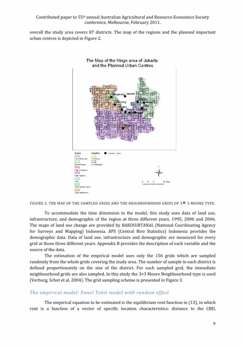
overall the study area covers 87 districts. The map of the regions and the planned important

urban centres is depicted in Figure 2.

FIGURE 3. THE MAP OF THE SAMPLED GRIDS AND THE NEIGHBOURHOOD GRIDS OF 3 3 MOORE TYPE.

To accommodate the time dimension in the model, this study uses data of land use,

infrastructure, and demographic of the region at three different years, 1995, 2000 and 2006.

The maps of land use change are provided by BAKOSURTANAL (National Coordinating Agency

for Surveys and Mapping) Indonesia. BPS (Central Biro Statistics) Indonesia provides the

demographic data. Data of land use, infrastructure and demographic are measured for every

grid at those three different years. Appendix B provides the description of each variable and the

source of the data.

The estimation of the empirical model uses only the 156 grids which are sampled

randomly from the whole grids covering the study area. The number of sample in each district is

defined proportionately on the size of the district. For each sampled grid, the immediate

neighbourhood grids are also sampled. In this study the 3×3 Moore Neighbourhood type is used

(Verburg, Schot et al. 2004). The grid sampling scheme is presented in Figure 3.

The empirical model: Panel Tobit model with random effect

The empirical equation to be estimated is the equilibrium rent function in (13), in which

rent is a function of a vector of specific location characteristics: distance to the CBD,



10

geographical conditions, and neighbourhood land use externalities. The equation will be defined

for each grid for different point of time t.

A proxy for development rent in (13) is the development proportion in each grid. The

small proportion of development in each grid implies that the particular grid is very less likely

to be developed or it has low development value. On the other hand, the higher the proportion

of development in a grid represents its potential for development or its high development value.

A non negative value of a grid development proportion measures the land consumption

for development in that grid. When the development carried out horizontally, the observed grid

development proportion captures well the amount of the development. Furthermore when the

land in a particular grid is fully developed, or the development proportion of that grid equals

one, it is still possible that more development occurs vertically, implying that the development

proportion is greater than one. However, this additional development cannot be observed

directly when the proportion reaches one. Therefore, Tobit Regression is used, where the data is

censored for value less than 0 and more than 1.

The empirical equation to be estimated is defined as follows:

:[∗�\,]� = ^[�\,]�_ + `[�\,]�, (18)

where `[�\,]�~S�0, bZ�. ^[�\,]� is the vector of land characteristics which are observed for all

cases, :[∗�\,]� is a latent variable measuring the observed development amount in grid �c, d� at

time t. The index �c, d� in (18) is the Cartesian coordinate for the position of the centre of the

sampled grid: �c, d� ∈ L, where L is the set of 156 sampled grids. The point of origin (0, 0) is the

location of the CBD. As mentioned earlier this empirical study uses three different years.

However, by assuming that the development decision accommodates the previous time

neighbourhood externalities, the time index is one less than the available time index. Thus, if e = 1,2,3 correspond to year 1995, 2000 and 2006 respectively, the time index defines in (18)

corresponds to e = 2,3.

The development proportion measuring the amount of development variable in (18) is

defined as a latent type of variable. It is observed for any proportion value between 0 and 1, and

it is censored for any value less than 0 or more than 1:

:[�\,]� = h 0 if :[∗�\,]� < 0:[∗�\,]� if 0 ≤ :[∗�\,]� ≤ 11 if :[∗�\,]� > 1 A. (19)

By the definition of :\][∗ in (18), the following holds:

:[�\,]� = h 0, if :[∗�\,]� < 0:[∗�\,]� = ^[�\,]�_ + `[�\,]�, if 0 ≤ :[∗�\,]� ≤ 11, if :[∗�\,]� > 1 A (20)

which is the definition of the Tobit Model for censored outcome (Long 1997). The latent

variable describes the amount of any occurred development :∗�\,]�, while the censored variable

defines the observed development which consumes previously open space or agricultural site



11

:∗�\,]�. Furthermore, since the sampled grids are drawn randomly from the overall grids which

cover the studied region, it is assumed that:

`[�\,]� = ��\,]� + >[�\,]�, (21)

where ��\,]�~c. cQ. S�0, bFZ� is the individual specific error for each grid �c, d� which is

independent of ^[�\,]�, and >[�\,]�~c. cQ. S�0, bEZ� is the idiosyncratic error. Therefore, the

particular model in (18) is defined as the Panel Tobit model with random effect. In the

definition of the error terms, bFZ is the panel level variance component which measures the

variability between grids or locations in the impact of the unmeasured time constant variables,

whereas bEZ measures the variability within a particular grid across time periods in the impact

of the unmeasured time-varying variables.

The independent variables

:\][∗ in (18) is a function of ^[�\,]� the vector of land characteristics for each grid �c, d� at

time t. The following land characteristic variables: distance to urban centre, green and social

externalities (in term of density) at time �e − 1� and conversion costs, are the elements of ^[�\,]�.

Distance to the CBD

This variable is defined as l (km) to represent the distance of the grid location to the

CBD, through the road network.

The Externalities

Household’s decision for the residential location is based on the neighbourhood

externalities that are observed at the previous time period. In this empirical study the average

density of a grid’s 3×3 Moore neighbour grids defines the neighbourhood externalities which

are enjoyed by the particular grid. There are two types of externalities considered, green and

social externalities. They are both functions of the neighbourhood density at the previous

period of time. The green type of externalities decreases in neighbourhood density, and the

social type of externalities increases in neighbourhood density. Both types of externalities in

(13) define the rent through the household’s utility, such that the increase in neighbourhood

density affects the utility in two ways: it decreases the utility through the green externalities

and it increases the utility through the social externalities. However, the rate of decrease in the

utility is higher than the rate of its increase, which motivates the use of different power to the

neighbourhood density. The powers used in this study are based on the restriction of the

parameter for both externalities defined in Caruso et al. (2007), power one for the green

externalities and the square root for the social externalities, which lead to their following

definitions:

[�\,]� = −SmDn�ceo[ ��\,]�, (22)

for the green neighbourhood externalities and

L[�\,]� = pSmDn�ceo[ ��\,]�, (23)



12

for the social neighbourhood externalities, where

SmDn�ceo[ ��\,]� = 18 r mDn�ceo[ ��\,]��\,]�∈s

mDn�ceo[ ��\,]�: the population density (people/square km) of grid �c, d� at time e − 1, and

S: the 8 grids as a set of 3 × 3 Moore Neigbhourhood of grid �c, d�.

The Cost of Conversion

The topographic condition of each grid represents the costs needed to convert the land

in that particular grid to be converted for development use. It is assumed that the grid with

mostly flat topographic condition needs less cost for conversion and more likely to be

developed than the grid with the other defined topographic conditions: hilly or swampy. The

following vector defines the topographic condition for the grid �c, d�:

uvw�\,]� = +xyzz{�\,]� |}~�w�\,]�,

The time index is omitted in this variable, since it is assumed there was no significant change in

the topographical condition through the years of observation. It is a 1 × 2 vector with two

dummy variables as its elements:

xyzz{�\,]� = @1, if grid �c, d� is dominated by mountain or hill0, otherwise A |}~�w�\,]� = @1, if grid �c, d� is dominated by swamp, river of lake0, otherwise A

If grid �c, d� is dominated by flat terrain, both of the indicator variables have 0 values.

The cost of conversion is also represented by the available utility or infrastructure in

that grid, which can be one of the following facilities: school, market, religious building,

government office, road, and electricity.

This variable is defined as:

�u��[�\,]� = @1, if utility is provided in grid �c, d� at time e0, otherwise A The matrix of independent variables

The above defined variables are the elements of matrix ^y�� in (18) such that:

^[�\,]� = � �[�\,]� [�\,]� L[�\,]�u��\,]� ��P[�\,]� 1�. (24)

4. THE RESULTS OF THE EMPIRICAL STUDY

The Generalized Least Square (GLS) estimators of the coefficients of the empirical model

in (18) are calculated using STATA. The output of the analysis is presented in Figure 4. In



13

overall the estimated coefficients for the model are jointly significant at 5% level of confidence

(see Wald Chi Square statistics: Wald chi2(6) in Figure 4). Thus, there is strong evidence that

the chosen independent variables can explain the amount of the occurred development very

well.

In addition to the overall significance of the model, the following statistics are provided

to analyse the significance of the panel setting of the model. The first statistic is the percent

contribution to the total variance of the panel level variance component (rho in Figure 4 ):

� = b�FZb�FZ + b�EZ = 0.87726 where b��Z = �c��<_>2 = 0.1853074

2 is the estimated panel level variance component and b�EZ = �c��<_DZ = 0.06931412 is the estimated overall variance component. The value of �

which is close to 1 defines the domination of the panel level variance component. It is supported

by the significance of the second statistic: chibar2,the likelihood ratio test statistic presented

below the analysis of variance table in Figure 4. The test reveals that the panel estimator is

significantly different from the pooled estimator. Furthermore, the estimated panel level

variance component which is significantly bigger than the estimated overall variance

component, indicates that the variability between grids or location due to the unmeasured time

constant variable is bigger than the variability within a location across time due to the

unmeasured time varying variable. It implies that the chosen independent variables explain

much the variability of development amount of a particular location across time, and the

between grids variability shows the significant difference among the location of the

development.



14

Random-effects tobit regression Number of obs = 320

Group variable: id Number of groups = 160

Random effects u_i ~ Gaussian Obs per group: min = 2

avg = 2.0

max = 2

Wald chi2(6) = 311.30

Log likelihood = 128.38743 Prob > chi2 = 0.0000

R | Coef. Std. Err. z P>|z| [95% Conf. Interval]

r | -2.89e-06 1.73e-06 -1.67 0.096 -6.29e-06 5.09e-07

G | .0000724 .0000208 -3.49 0.000 -.0001131 -.0000317

S | .0132007 .0020903 6.32 0.000 .0091038 .0172976

hilly | -.0635602 .0325437 -1.95 0.051 -.1273446 .0002242

swampy | -.1416495 .123776 -1.14 0.252 -.3842461 .100947

util | .2644578 .0471819 5.61 0.000 .1719828 .3569327

_cons | -.0362003 .0954222 -0.38 0.704 -.2232244 .1508238

-------------+----------------------------------------------------------------

/sigma_u | .1853074 .0122569 15.12 0.000 .1612844 .2093305

/sigma_e | .0693141 .0043486 15.94 0.000 .0607911 .0778372

-------------+----------------------------------------------------------------

rho | .87726 .020564 .8322483 .9130388

Likelihood-ratio test of sigma_u=0: chibar2(01)= 194.43 Prob>=chibar2 = 0.000

Observation summary: 47 left-censored observations

269 uncensored observations

4 right-censored observations

FIGURE 4. THE STATA OUTPUT OF GLS ESTIMATORS OF PANEL TOBIT WITH RANDOM EFFECTS MODEL.

Before analysing the estimated coefficients, there are two interested outcome based on

the estimators of the Tobit model: (1) the amount of any occurred development (latent variable: :∗); and (2) the observed or the censored development proportion in term of land consumption

(:), thus the expected value and the marginal effect of this model have different form for each

outcome (Greene 2008). Furthermore, since the Tobit model used in this study involves a

polynomial term of independent variable (SmDn�ceo in the externalities variables and L), the

partial derivative for this variable will be different to the linearly independent variable. Table 1

presents all the formulations of the expected value and the marginal effect.

Based on the formulation on Table 1, and the estimated coefficients on Figure 4, the

marginal effect of each independent variable is calculated and presented in Table 2. Each value

defines how the change of the particular variable affecting the development amount, both the

latent and the censored ones. In general, the directions of the marginal effect of all independent

variables are in accordance with the urban theory. The further the distance from the CBD (l)

and the topographical condition others than flat (Hilly and Swampy) decrease the development

amount. The higher the externalities offered by the neighbourhood and the provided utility

increase the development amount.



15

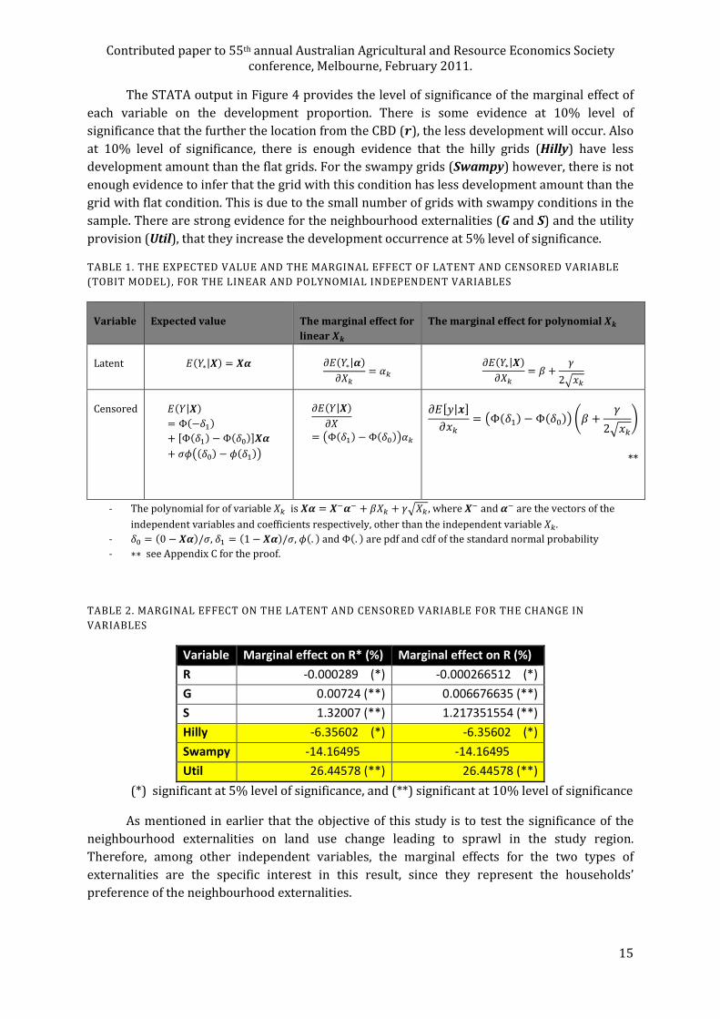
The STATA output in Figure 4 provides the level of significance of the marginal effect of

each variable on the development proportion. There is some evidence at 10% level of

significance that the further the location from the CBD (l), the less development will occur. Also

at 10% level of significance, there is enough evidence that the hilly grids (Hilly) have less

development amount than the flat grids. For the swampy grids (Swampy) however, there is not

enough evidence to infer that the grid with this condition has less development amount than the

grid with flat condition. This is due to the small number of grids with swampy conditions in the

sample. There are strong evidence for the neighbourhood externalities (G and S) and the utility

provision (Util), that they increase the development occurrence at 5% level of significance.

TABLE 1. THE EXPECTED VALUE AND THE MARGINAL EFFECT OF LATENT AND CENSORED VARIABLE

(TOBIT MODEL), FOR THE LINEAR AND POLYNOMIAL INDEPENDENT VARIABLES

Variable Expected value The marginal effect for

linear ^

The marginal effect for polynomial ^

Latent ¡�A;∗|^� = ^£ ¤¡�A;∗|£�¤¥¦ = �¦ ¤¡�A;∗|^�¤¥¦ = � + �2§¨¦

Censored ¡�A;|^�= Φ�−©��+ Φ�©�� − Φ�©��^£+ b62�©�� − 6�©��3

¤¡�A;|^�¤¥= 2Φ�©�� − Φ�©��3�¦

¤¡Ao|ª�¤¨¦ = 2Φ�©�� − Φ�©��3 «� + �2§¨¦¬

**

- The polynomial for of variable ¥¦ is ^£ = ^ £ + �¥¦ + �§¥¦ , where ^ and £ are the vectors of the

independent variables and coefficients respectively, other than the independent variable ¥¦ .

- ©� = �0 − ^£�/b, ©� = �1 − ^£�/b, 6�. � and Φ�. � are pdf and cdf of the standard normal probability

- ∗∗ see Appendix C for the proof.

TABLE 2. MARGINAL EFFECT ON THE LATENT AND CENSORED VARIABLE FOR THE CHANGE IN

VARIABLES

Variable Marginal effect on R* (%) Marginal effect on R (%)

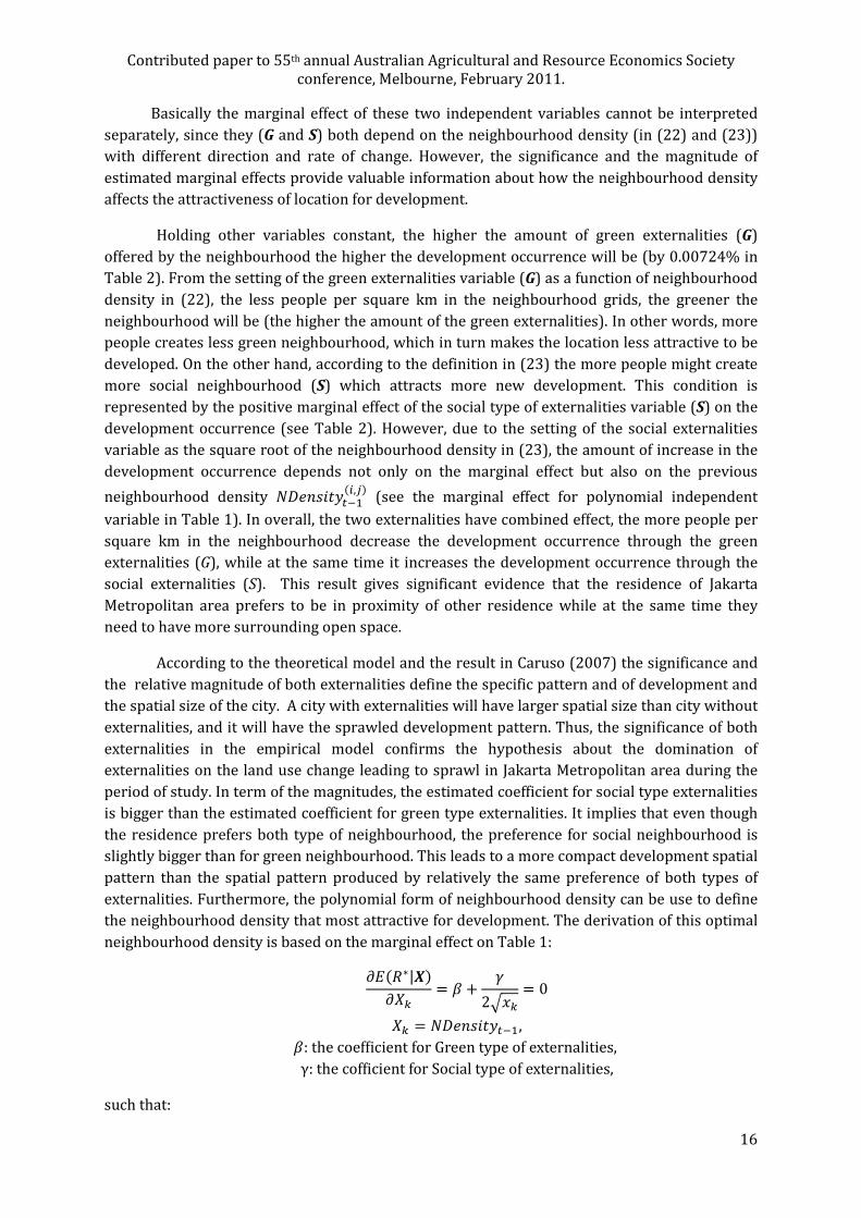
R -0.000289 (*) -0.000266512 (*)

G 0.00724 (**) 0.006676635 (**)

S 1.32007 (**) 1.217351554 (**)

Hilly -6.35602 (*) -6.35602 (*)

Swampy -14.16495 ( -14.16495 (

Util 26.44578 (**) 26.44578 (**)

(*) significant at 5% level of significance, and (**) significant at 10% level of significance

As mentioned in earlier that the objective of this study is to test the significance of the

neighbourhood externalities on land use change leading to sprawl in the study region.

Therefore, among other independent variables, the marginal effects for the two types of

externalities are the specific interest in this result, since they represent the households’

preference of the neighbourhood externalities.



16

Basically the marginal effect of these two independent variables cannot be interpreted

separately, since they (G and S) both depend on the neighbourhood density (in (22) and (23))

with different direction and rate of change. However, the significance and the magnitude of

estimated marginal effects provide valuable information about how the neighbourhood density

affects the attractiveness of location for development.

Holding other variables constant, the higher the amount of green externalities (G)

offered by the neighbourhood the higher the development occurrence will be (by 0.00724% in

Table 2). From the setting of the green externalities variable (G) as a function of neighbourhood

density in (22), the less people per square km in the neighbourhood grids, the greener the

neighbourhood will be (the higher the amount of the green externalities). In other words, more

people creates less green neighbourhood, which in turn makes the location less attractive to be

developed. On the other hand, according to the definition in (23) the more people might create

more social neighbourhood (S) which attracts more new development. This condition is

represented by the positive marginal effect of the social type of externalities variable (S) on the

development occurrence (see Table 2). However, due to the setting of the social externalities

variable as the square root of the neighbourhood density in (23), the amount of increase in the

development occurrence depends not only on the marginal effect but also on the previous

neighbourhood density SmDn�ceo[ ��\,]� (see the marginal effect for polynomial independent

variable in Table 1). In overall, the two externalities have combined effect, the more people per

square km in the neighbourhood decrease the development occurrence through the green

externalities (G), while at the same time it increases the development occurrence through the

social externalities (S). This result gives significant evidence that the residence of Jakarta

Metropolitan area prefers to be in proximity of other residence while at the same time they

need to have more surrounding open space.

According to the theoretical model and the result in Caruso (2007) the significance and

the relative magnitude of both externalities define the specific pattern and of development and

the spatial size of the city. A city with externalities will have larger spatial size than city without

externalities, and it will have the sprawled development pattern. Thus, the significance of both

externalities in the empirical model confirms the hypothesis about the domination of

externalities on the land use change leading to sprawl in Jakarta Metropolitan area during the

period of study. In term of the magnitudes, the estimated coefficient for social type externalities

is bigger than the estimated coefficient for green type externalities. It implies that even though

the residence prefers both type of neighbourhood, the preference for social neighbourhood is

slightly bigger than for green neighbourhood. This leads to a more compact development spatial

pattern than the spatial pattern produced by relatively the same preference of both types of

externalities. Furthermore, the polynomial form of neighbourhood density can be use to define

the neighbourhood density that most attractive for development. The derivation of this optimal

neighbourhood density is based on the marginal effect on Table 1:

¤¡�A:∗|^�¤¥¦ = � + �2§¨¦ = 0

¥¦ = SmDn�ceo[ �, �: the coef¯icient for Green type of externalities, γ: the cof¯icient for Social type of externalities,

such that:



17

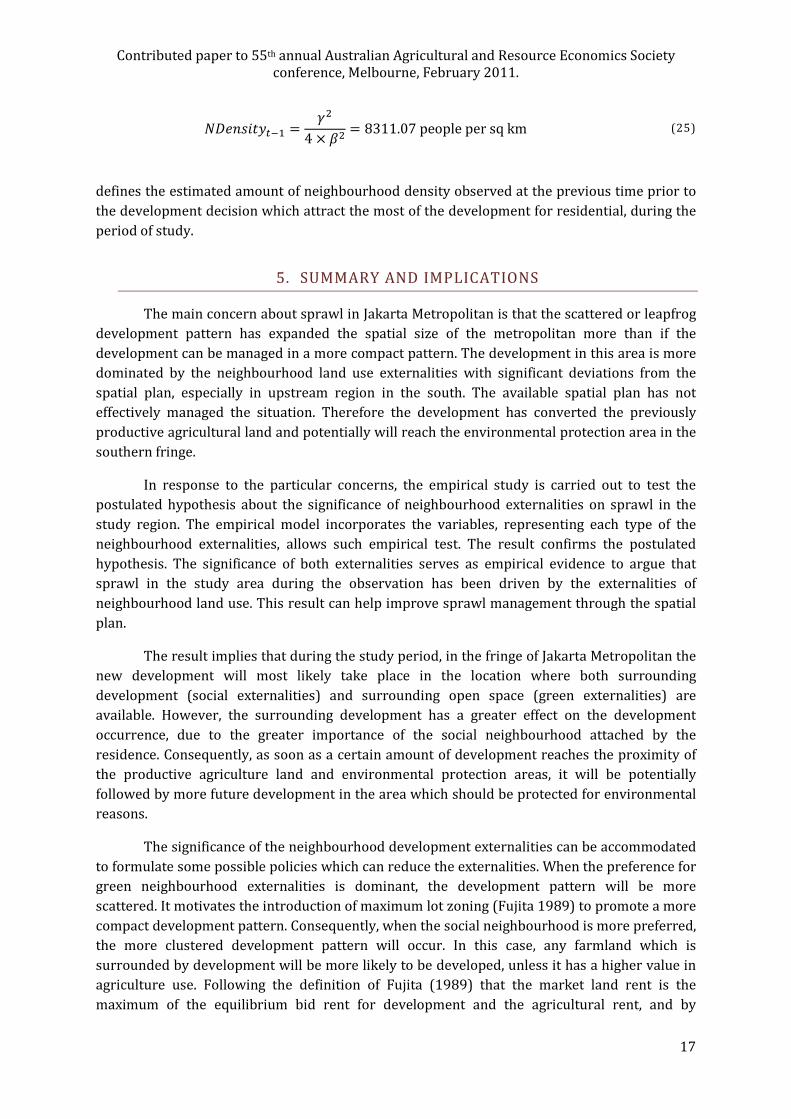
SmDn�ceo[ � = �Z4 × �Z = 8311.07 people per sq km (25)

defines the estimated amount of neighbourhood density observed at the previous time prior to

the development decision which attract the most of the development for residential, during the

period of study.

5. SUMMARY AND IMPLICATIONS

The main concern about sprawl in Jakarta Metropolitan is that the scattered or leapfrog

development pattern has expanded the spatial size of the metropolitan more than if the

development can be managed in a more compact pattern. The development in this area is more

dominated by the neighbourhood land use externalities with significant deviations from the

spatial plan, especially in upstream region in the south. The available spatial plan has not

effectively managed the situation. Therefore the development has converted the previously

productive agricultural land and potentially will reach the environmental protection area in the

southern fringe.

In response to the particular concerns, the empirical study is carried out to test the

postulated hypothesis about the significance of neighbourhood externalities on sprawl in the

study region. The empirical model incorporates the variables, representing each type of the

neighbourhood externalities, allows such empirical test. The result confirms the postulated

hypothesis. The significance of both externalities serves as empirical evidence to argue that

sprawl in the study area during the observation has been driven by the externalities of

neighbourhood land use. This result can help improve sprawl management through the spatial

plan.

The result implies that during the study period, in the fringe of Jakarta Metropolitan the

new development will most likely take place in the location where both surrounding

development (social externalities) and surrounding open space (green externalities) are

available. However, the surrounding development has a greater effect on the development

occurrence, due to the greater importance of the social neighbourhood attached by the

residence. Consequently, as soon as a certain amount of development reaches the proximity of

the productive agriculture land and environmental protection areas, it will be potentially

followed by more future development in the area which should be protected for environmental

reasons.

The significance of the neighbourhood development externalities can be accommodated

to formulate some possible policies which can reduce the externalities. When the preference for

green neighbourhood externalities is dominant, the development pattern will be more

scattered. It motivates the introduction of maximum lot zoning (Fujita 1989) to promote a more

compact development pattern. Consequently, when the social neighbourhood is more preferred,

the more clustered development pattern will occur. In this case, any farmland which is

surrounded by development will be more likely to be developed, unless it has a higher value in

agriculture use. Following the definition of Fujita (1989) that the market land rent is the

maximum of the equilibrium bid rent for development and the agricultural rent, and by



18

assuming that the rent to agriculture use initially exceeds the rent to development until the

value of development use increases which lead to conversion (Livanis, Moss et al. 2006), the

higher the value of land for agricultural use, the less will be its probability to be developed.

Thus, to reduce this type of externality, the agricultural zoning, or any exclusive rights for the

farmer to increase the land productivity can be introduced.

In the study region, since both types of externalities are significant, the combination of

both policies should be implemented. Particularly, the maximum lot size zoning can be

implemented by maintaining the boundary of urban area at a certain distance from the CBD.

Therefore the development can be contained and limited such that it will not reach the

environmental protection zone in the fringe. This particular distance can be seen as an inner

metropolitan boundary. For the study region, based on the empirical result, this distance can be

defined as the distance where the optimal neighbourhood density achieved: the density where

the neighbourhood externalities preferred the most. With the introduction of this inner

boundary, the average space consumed for future residential development outside the inner

boundary has to be set below certain lot size (maximum lot) which optimized the

neighbourhood density (see (25)). Together with better infrastructure provision inside the

boundary, with the social neighbourhood are slightly more preferred than the green

neighbourhood, this type of urban containment policy will not necessarily decrease the

residence’s utility. However, whether the sprawl or a more compact spatial development

pattern is socially optimum for the study region is beyond the scope of this study.



19

APPENDIX A THE DERIVATIVE OF THE URBAN FRINGE BOUNDARY DISTANCE WITH RESPECT TO

THE EXTERNALITIES

The following definitions are the equilibrium bid rent function and the urban fringe boundary

distance:

=∗2; − <�, >, ��3 = ��F �H+J�⁄ �; − <��1+J� �H+J�⁄ D−E �H+J�⁄

and

�T =1< 2; − Φ

�β+c� �1+c�⁄ β

−�β+c� �1+c�⁄ α−α �1+c�⁄ DE �1+J�⁄ 3

respectively. By assuming < = 1 without losing generality, the following urban fringe boundary

distance is defined as function of 5, which measures the extent of externalities:

�T�5� = ; − µ�5� = ; − µ1�5�µ2�5�

µ1�5� = 2Φ�−13�β+c� �1+c�⁄

µ2�5� = 2�−1DE31 �1+J�⁄

It will be proven that �T is an increasing function of c. The first derivative of µ1�5� and µ2�5�

with respect to c:

¤µ1�5�¤5 = µ1�5� 1 − β�1 + c�2ln2 Φ�−13

and

¤µ2�5�¤5 = µ2�5� −1�1 + c�2ln2�−1DE3

respectively. It leads to the following derivative:

Qµ�5�Q5 = µ1�5� ¤µ2�5�¤5 + µ2�5� ¤µ1�5�¤5 = µ�5� ¶ 1 − β�1 + c�2ln2 Φ�−13 −

1�1 + c�2ln2�−1DE3·

With the parameter conditions that � + � = 1, the following holds:

Qµ�5�Q5 = µ�5� 1�1 + c�2+� ln2 Φ�−13 − ln �−1 − >, < 0,

in which ln2 Φ�−13 > 0, ln �−1 > 0 due to the assumptions 0 < � ≤ 1 and 0 < � ≤ 1, and > > 0

dominates the first and the second terms. The above result implies that:

Q�T�5�Q5 = −Qµ�5�Q5 > 0

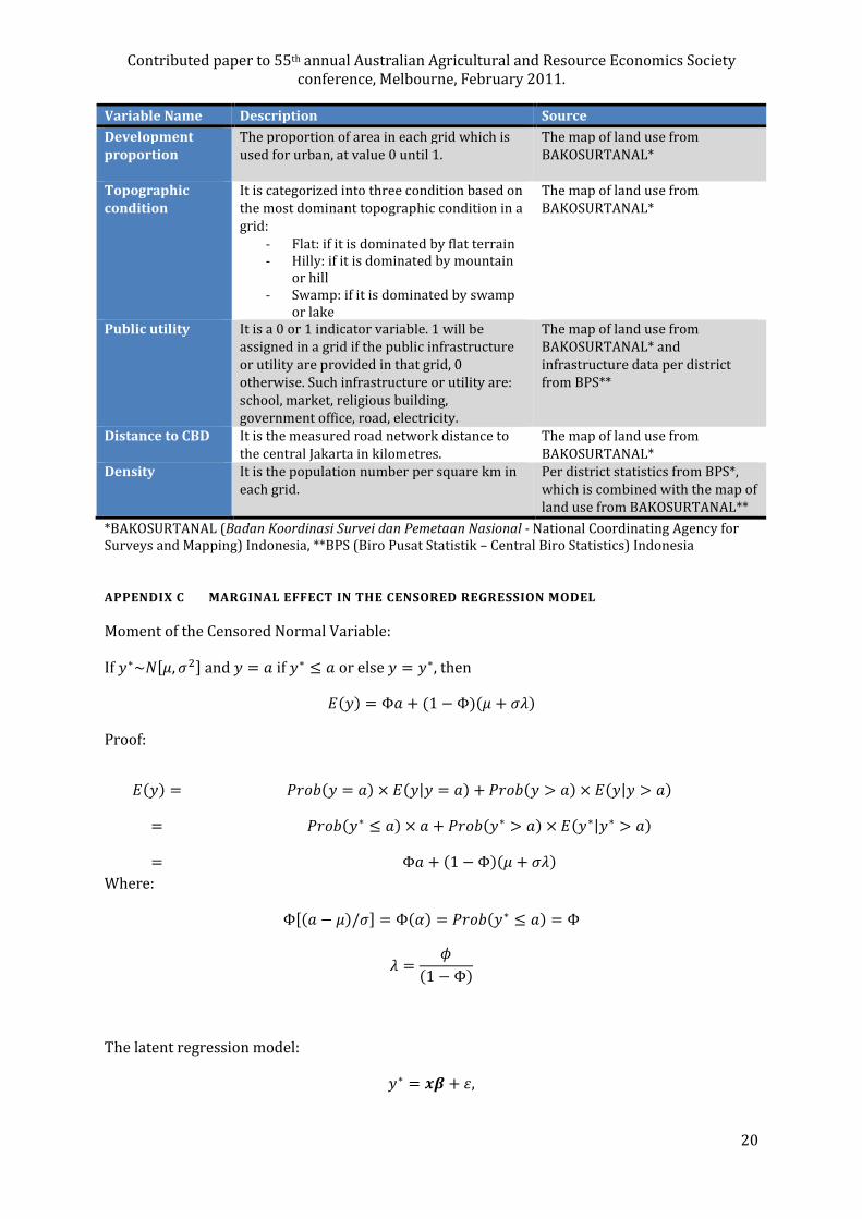
APPENDIX B THE DESCRIPTION OF THE VARIABLES



20

Variable Name Description Source

Development

proportion

The proportion of area in each grid which is

used for urban, at value 0 until 1.

The map of land use from

BAKOSURTANAL*

Topographic

condition

It is categorized into three condition based on

the most dominant topographic condition in a

grid:

- Flat: if it is dominated by flat terrain

- Hilly: if it is dominated by mountain

or hill

- Swamp: if it is dominated by swamp

or lake


BAKOSURTANAL*

Public utility It is a 0 or 1 indicator variable. 1 will be

assigned in a grid if the public infrastructure

or utility are provided in that grid, 0

otherwise. Such infrastructure or utility are:

school, market, religious building,

government office, road, electricity.


BAKOSURTANAL* and

infrastructure data per district

from BPS**

Distance to CBD It is the measured road network distance to

the central Jakarta in kilometres.


BAKOSURTANAL*

Density It is the population number per square km in

each grid.

Per district statistics from BPS*,

which is combined with the map of

land use from BAKOSURTANAL**

*BAKOSURTANAL (Badan Koordinasi Survei dan Pemetaan Nasional - National Coordinating Agency for

Surveys and Mapping) Indonesia, **BPS (Biro Pusat Statistik – Central Biro Statistics) Indonesia

APPENDIX C MARGINAL EFFECT IN THE CENSORED REGRESSION MODEL

Moment of the Censored Normal Variable:

If o∗~S¸, bZ� and o = < if o∗ ≤ < or else o = o∗, then

¡�o� = Φ< + �1 − Φ��¸ + b��

Proof:

¡�o� = ¹�º��o = <� × ¡�Ao|o = <� + ¹�º��o > <� × ¡�Ao|o > <�

= ¹�º��o∗ ≤ <� × < + ¹�º��o∗ > <� × ¡�Ao∗|o∗ > <�

= Φ< + �1 − Φ��¸ + b��

Where:

Φ�< − ¸�/b� = Φ�� = ¹�º��o∗ ≤ <� = Φ

� = 6�1 − Φ�

The latent regression model:

o∗ = ª_ + »,



21

and observed dependent variable, o = < if o∗ ≤ < , o = � if o∗ ≥ � and o = o∗ otherwise. a and b

are constant.

Let 6�»� and Φ�»� as the density and cdf of ». Assume that »~S�0, bZ�. For the non linearity of x

in the Tobit model: ¨¦ appears in the equation two times with power one and 0.5 respectively.

ª_ = ª _ + �¦�¨¦ + �¦Z§¨¦ , (**)

where ª and _ are the vectors of the independent variables and coefficients respectively,

other than the independent variable k. The marginal effect on the censored outcome:

¤¡Ao|ª�¤¨¦ = Φ�δ� «�¦� + �¦Z2§¨¦¬, where: © = ª_¾ and (**) holds

Proof:

By definition (Greene 2008):

¡Ao|ª� = <¹�º�Ao∗ ≤ <|ª� + �¹�º�Ao∗ ≥ �|ª� + ¹�º�A< < o∗ < �|ª�¡A< < o∗ < �|ª�

Let:

©¿ = �< − ª_�b , ©À = �� − ª_�b and ** holds. Then:

¡Ao|ª� = <Φ�©¿� + �21 − Φ�©À�3 + 2Φ�©À� − Φ�©¿�3¡A< < o∗ < �|ª�.

Because:

o∗ = ª_ + b�o∗ − ª_�/b�, The conditional mean may be written as:

¡Ao∗|< < o∗ < �� = ª_ + b¡ ¶Ao∗ − ª_b B < − ª_b < o∗ − ª_b < � − ª_b ·

= ª_ + b O �»/b�6�»/b�Φ�©À� − Φ�©¿� Q Á»bÂÃÄÃÅ

Collecting terms:

¡Ao|ª� = <Φ�©¿� + �21 − Φ�©À�3 + 2Φ�©À� − Φ�©¿�3ª_ + b O Á»bÂ 6 Á»bÂ Q Á»bÂÃÄÃÅ

Now, differentiate with respect to ¨¦.

The complication is the last term, for which the differentiation is with respect to the limits of

integration. The Leibnitz’s theorem is used and use the assumption that 6�»� does not involve ª.



22

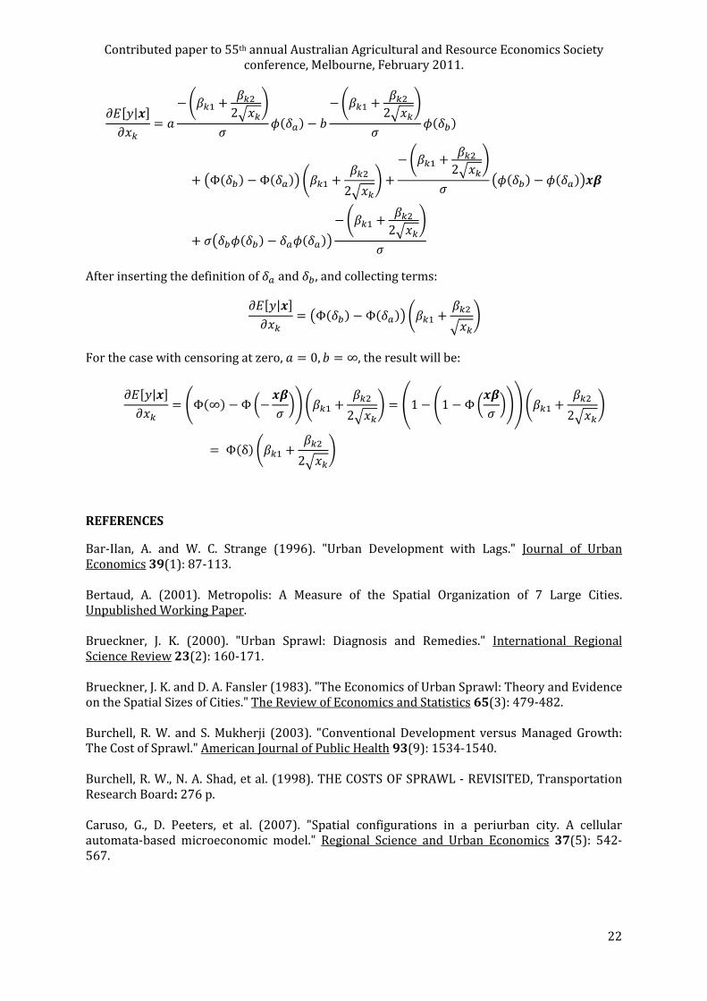
¤¡Ao|ª�¤¨¦ = < − «�¦� + �¦Z2§¨¦¬b 6�©¿� − � − «�¦� + �¦Z2§¨¦¬

b 6�©À�+ 2Φ�©À� − Φ�©¿�3 «�¦� + �¦Z2§¨¦¬ + − «�¦� + �¦Z2§¨¦¬

b 26�©À� − 6�©¿�3ª_+ b2©À6�©À� − ©¿6�©¿�3 − «�¦� + �¦Z2§¨¦¬

b

After inserting the definition of ©¿ and ©À , and collecting terms:

¤¡Ao|ª�¤¨¦ = 2Φ�©À� − Φ�©¿�3 «�¦� + �¦Z§¨¦¬

For the case with censoring at zero, < = 0, � = ∞, the result will be:

¤¡Ao|ª�¤¨¦ = ÇΦ�∞� − Φ È− ª_b ÉÊ «�¦� + �¦Z2§¨¦¬ = Ë1 − Ç1 − Φ Èª_b ÉÊÌ «�¦� + �¦Z2§¨¦¬= Φ�δ� «�¦� + �¦Z2§¨¦¬

REFERENCES

Bar-Ilan, A. and W. C. Strange (1996). "Urban Development with Lags." Journal of Urban

Economics 39(1): 87-113.

Bertaud, A. (2001). Metropolis: A Measure of the Spatial Organization of 7 Large Cities.

Unpublished Working Paper.

Brueckner, J. K. (2000). "Urban Sprawl: Diagnosis and Remedies." International Regional

Science Review 23(2): 160-171.

Brueckner, J. K. and D. A. Fansler (1983). "The Economics of Urban Sprawl: Theory and Evidence

on the Spatial Sizes of Cities." The Review of Economics and Statistics 65(3): 479-482.

Burchell, R. W. and S. Mukherji (2003). "Conventional Development versus Managed Growth:

The Cost of Sprawl." American Journal of Public Health 93(9): 1534-1540.

Burchell, R. W., N. A. Shad, et al. (1998). THE COSTS OF SPRAWL - REVISITED, Transportation

Research Board: 276 p.

Caruso, G., D. Peeters, et al. (2007). "Spatial configurations in a periurban city. A cellular

automata-based microeconomic model." Regional Science and Urban Economics 37(5): 542-

567.



23

Douglass, M. (2005). Globalization, Mega-projects and the Environment: Urban Form and Water

in Jakarta. Internatial Dialogic Conference on Global Cities: Water, Infrastructure and

Environment. The UCLA Globalization Research Center - Africa.

Ewing, R. H. (2008). Characteristics, Causes, and Effects of Sprawl: A Literature Review. Urban

Ecology: 519-535.

Firman, T. (1997). "Land Conversion and Urban Development in the Northern Region of West

Java, Indonesia." Urban Studies 34(7): 1027-1046.

Fujita, M. (1976). "Spatial patterns of urban growth: Optimum and market." Journal of Urban

Economics 3(3): 209-241.

Fujita, M. (1989). Urban economic theory : land use and city size / Masahisa Fujita. Cambridge

[Cambridgeshire] ; New York :, Cambridge University Press.

Galster, G., R. Hanson, et al. (2001). "Wrestling Sprawl to the Ground: Defining and measuring an

elusive concept." Housing Policy Debate 12(4): 681-717.

Greene, W. H. (2008). Econometric analysis. Upper Saddle River, N.J., Pearson/Prentice Hall.

Irwin, E. G. and N. E. Bockstael (2002). "Interacting agents, spatial externalities and the

evolution of residential land use patterns." J Econ Geogr 2(1): 31-54.

Irwin, E. G. and N. E. Bockstael (2004). "Land use externalities, open space preservation, and

urban sprawl." Regional Science and Urban Economics 34(6): 705-725.

Livanis, G., C. B. Moss, et al. (2006). "Urban sprawl and farmland prices." 88(4): 915-929.

Long, J. S. (1997). Regression models for categorical and limited dependent variables. Thousand

Oaks :, Sage Publications.

Lowry, I. S. (1988). Planning for Urban Sprawl. Transportation Research Board Special Report

No 220: 275 - 312.

Mills, D. E. (1981). "Growth, speculation and sprawl in a monocentric city." Journal of Urban

Economics 10(2): 201-226.

Ministry of Department of Public Works, R. (2006). Penjelasan Menteri Pekerjaan Umum

Mengenai Rencana Tata Ruang Kawasan Jabodetabek Punjur Sebagai Masukan untuk RUU

Pemerintahan Provinsi Daerah Khusus Ibukota Negara Republik Indonesia. Jakarta, Departemen

Pekerjaan Umum Republik Indonesia.

Nechyba, T. J. and R. P. Walsh (2004). "Urban Sprawl." The Journal of Economic Perspectives

18(4): 177-200.

Sierra Club (1998). The Dark SIde of the American Dream: The Costs and Consequences of

Suburban Sprawl, Challenge to Sprawl Campaign. College Park, MD. undated.

Verburg, P. H., P. P. Schot, et al. (2004). "Land use change modelling: current practice and

research priorities." GeoJournal 61(4): 309-324.

Winarso, H. and T. Firman (2002). "Residential land development in Jabotabek, Indonesia:

triggering economic crisis?" Habitat International 26(4): 487-506.



24

the extent of sprawl in the fringe of jakarta metropolitan area from the

Documents