the extensive margin of exporting products: the continuum...

The Extensive Margin of Exporting Products:The Continuum Case∗

Costas Arkolakis‡

Yale University, CESifo and NBER

Marc-Andreas Muendler¶

UC San Diego, CESifo and NBER

First version: November 13, 2007This version: August 3, 2011

Abstract

We present a heterogeneous-firm model with product choice in continuous space. The con-tinuum model yields similar estimation equations to a companion paper in discrete space andalso generates the documented empirical regularities within and across firms (Arkolakis andMuendler 2010). In a generalization, we consider a cannibalization effect, by which a firmloses infra-marginal sales as it adds additional products in a market. To fit empirical relation-ships more closely, we allow for product sales that drop off faster than log linearly as the firmadds additional products. Estimates of the key entry cost parameters in the generalized modelconfirm those in our more parsimonious model: firms face a strong decline in product saleswith scope but market-specific entry costs drop fast so that wide-scope exporters sell theirlowest-selling products in minor amounts.Keywords: International trade; heterogeneous firms; multi-product firms; firm and productpanel data; BrazilJEL Classification: F12, L11, F14

∗We thank David Atkin, Thomas Chaney, Arnaud Costinot, Don Davis, Gilles Duranton, Jonathan Eaton, ElhananHelpman, Kalina Manova, Gordon Hanson, Lorenzo Caliendo, Sam Kortum, Giovanni Maggi, Marc Melitz, PeterNeary, Jim Rauch, Steve Redding, Kim Ruhl, Peter Schott, Daniel Trefler and Jon Vogel as well as several seminarand conference participants for helpful comments and discussions. Roberto Alvarez kindly shared Chilean exporterand product data for the year 2000, for which we report comparable results to our Brazilian findings in an onlineData Appendix at URL econ.ucsd.edu/muendler/research. Oana Hirakawa and Olga Timoshenko provided excellentresearch assistance. Muendler and Arkolakis acknowledge NSF support (SES-0550699 and SES-0921673) with grati-tude. A part of this paper was written while Arkolakis visited the University of Chicago, whose hospitality is gratefullyacknowledged.

‡[email protected] (www.econ.yale.edu/∼ka265).¶[email protected] (www.econ.ucsd.edu/muendler). Ph: +1 (858) 534-4799.

1

1 Introduction

Market entry costs are a key component in recent trade theory with heterogeneous firms. To assess

the relative magnitudes and relevance of entry costs components, we study multi-product exporters.

Multi-product exporters face different entry cost components when they enter markets and when

they widen their local product scope. In this paper, we present a generalized model of multi-product

exporters set in continuous product space. We allow for two additional components of market entry

costs compared to a companion paper in discrete product space (Arkolakis and Muendler 2010).

We consider a cannibalization effect, by which additional products reduce the sales of a firm’s

infra-marginal products; and we model product sales that drop with scope faster than log linearly to

fit empirical relationships more closely. We show that continuous product space delivers compact

theoretical relationships for empirical work, even though the number of products is countable in

the data.

Our model has heterogeneous firms and products, where firms face destination-specific local

entry costs for each of their products. Replicating our model for countably many products (Arko-

lakis and Muendler 2010), the model in this paper rests on a single source of firm heterogeneity:

productivity. Firms face declining efficiency in producing their less successful products, similar to

Eckel and Neary (2010) and Mayer, Melitz and Ottaviano (2011). Our setup extends the Melitz

(2003) framework to the multi-product setting where the firm decides along three export margins:

its entry into export destinations at a first extensive margin, its exporter scope (the number of prod-

ucts) in a destination at a second extensive margin, and its individual product sales in a destination

at the residual intensive margin. Our generalized model of multi-product exporters continues to

preserve predictions of previous trade theory. At the firm level, the model reproduces predictions

of Melitz (2003) and Chaney (2008) for the upper tail of the total sales distribution. At the country

level, our model generates a gravity equation for bilateral trade flows where the Pareto shape pa-

rameter plays a similar role as the Frechet shape parameter in Eaton, Kortum and Kramarz (2010),

and fixed market entry costs affect bilateral trade.

A parametric specification of our model generates a relationship between a product’s sales,

exporter scope and the product’s local sales rank, where product sales drop off faster than log

linearly in the product’s sales rank. When estimated, this relationship yields coefficient estimates

for the relevant market entry cost components. We use three-dimensional panel data of Brazilian

manufacturing producers, their destination markets and their products at the Harmonized System

2

(HS) 6-digit level as in Arkolakis and Muendler (2010). We then compare the results for this

sample to evidence from a sample of Chilean manufacturing producers and a sample of Brazilian

commercial intermediaries selling manufactures.

For Brazilian manufacturing producers, our non-linear least squares estimates confirm the more

restrictive ones from Arkolakis and Muendler (2010), and we find estimates for Chilean manufac-

turing producers to be close to the ones for Brazilian producers. Our non-linear estimates suggest

that incremental local entry costs drop at an elasticity of around −1.4 when producers introduce

additional products in a market where they are present. But firm-product efficiency drops off even

faster with an elasticity of around 2.6 at the sample mean, as producers introduce products further

away from their core competency. Adding the two fixed scope cost components, there are net

overall diseconomies of scope with a scope elasticity of around 1.2, similar to what we find in our

companion paper (Arkolakis and Muendler 2010).1

Our generalized estimates show that the simpler model in Arkolakis and Muendler (2010)

approximates main parameters reasonably well for manufacturing producers. Manufacturers are

the focus of much of the related empirical literature (Eaton, Kortum and Kramarz 2004, Bernard,

Redding and Schott 2011, e.g.). For commercial intermediaries, however, the non-log-linearity

in product introduction costs matters considerably: the according scope elasticity estimate would

be downward biased by almost 40 percent in the more restrictive log-linear estimation model.

Our evidence suggests that the relevant curvature in product introduction costs mainly stems from

products with minor sales. The existence of products with minor sales is, in turn, consistent with

the main mechanism of our theory. In our model, highly productive wide-scope firms overcome

local entry costs for their lowest-selling products relatively easily but they face fast increasing

marginal production costs away from core competency. Together, these two features explain why

sales of the lowest-selling products are minor at wide-scope firms.

Our nested demand system is based on conventional constant elasticities of substitution (CES)

in continuous product space and can provide an alternative multi-product framework compared

to the influential work by Bernard, Redding and Schott (2011 and 2011), who also use contin-

uous product space. Similar to Feenstra and Ma (2008), our model allows for a cannibalization

effect. In contrast to our CES framework with monopolistic competition, however, Feenstra and

Ma (2008) consider a countable number of firms and find a varying cannibalization effect to yield

1The cannibalization effect augments the costs of a wider exporter scope in addition, but we do not attempt toestimate this demand-side aspect using firm-level supply data.

3

a well defined exporter scope optimum in the absence of diseconomies of scope on the cost side.

A countable number of firms with product-market power, however, does not lead to closed-form

estimation relationships. Similar to recent work by Mayer et al. (2011), the parametric specifi-

cation of our model generates a non-log-linear relationship between firm-product sales and the

product rank. Beyond that similarity, the Mayer et al. (2011) framework complements our model

in demonstrating how variable markups further improve specific predictions.

The remainder of this paper is organized as follows. We introduce the general model in Sec-

tion 2. In Section 3 we derive predictions for bilateral trade under a Pareto distribution and adopt

parametric functional forms for firm-level predictions. We obtain structural estimates of entry cost

parameters in Section 4. Section 5 concludes. Some details on derivations and data sources are

relegated to the Appendix.

2 A Model of Exporter Scope and Product Scale

Our model has heterogeneous firms that sell a finite measure of products in the markets where

they enter. Our continuum model rests on a single source of firm heterogeneity and there are

three key ingredients, just as in the corresponding model with countably many discrete products:

a firm’s productivity explains total sales of the firm’s products worldwide; firm-product specific

efficiency determines individual product sales worldwide; and a firm repeatedly incurs fixed entry

costs per product destination by destination. Beyond the benchmark specification in Arkolakis and

Muendler (2010), we consider a cannibalization effect by which additional products reduce the

sales of a firm’s infra-marginal products and we allow for product sales that drop off faster than

log linearly as a firm adds products.

2.1 Consumers

There are N countries. We label the source country of an export shipment with s and the export

destination with d. There is a measure of Ld consumers at destination d. Consumers have sym-

metric preferences with a constant elasticity of substitution σ over a continuum of varieties. A

conventional “variety” becomes the product composite

Xsd(ω) ≡

[∫ Gsd(ω)

g

xsd(ω; g)ε−1ε dg

] εε−1

4

in continuous product space, where Gsd(ω) is the measure of products that firm ω sells in country

d, and xsd(ω; g) is the quantity of product g that consumers consume. In marketing terminology,

the product composite is a firm’s product line or product mix. The index numbers g start at some

initial index g.2 The elasticity of substitution ε is constant across products within the product line

and possibly different from σ. We assume that every product line is uniquely offered by a single

firm, but a firm may ship different product lines to different destinations.

The set of product lines shipped from source country s to destination d for consumption is Ωsd.

So the consumer’s utility at destination d is N∑s=1

∫ω∈Ωsd

[∫ Gsd(ω)

g


] εε−1

σ−1σ

dω

σ

σ−1

where ε > 1, σ > 1, ε = σ. (1)

Allanson and Montagna (2005) use a similar nested utility to study implications of the product

life-cycle for market structure. Atkeson and Burstein (2008) adopt a similar nested CES form in

a heterogeneous-firms model of trade but do not consider multi-product firms. The specification

generalizes monopolistic-competition models of trade (such as Krugman 1980).3 For preferences

to be well defined, we require that ε > 1 and σ > 1. Subsequent derivations do not materially

differ if we assume that products within a product line are more substitutable among each other

than with outside products (ε > σ > 1), or less substitutable (σ > ε > 1). Evidence in Broda and

Weinstein (2007) suggests that products are stronger substitutes within brands than across brands

so we consider ε > σ > 1 our main case.4

The consumer receives per-capita income yd = wd + πd, where wd is the wage for labor,

inelastically supplied to producers in country d, and πd ≡∫ N

ω=1πsdω/Ld is the consumer’s share in

total profits earned by the country’s producers. Country d’s total income is ydLd. The consumer’s

2When we turn to parametric estimation equations we set g = 1 similar to discrete product space.3The counterpart to (1) in discrete product space are consumer preferences at d N∑

s=1

∫ω∈Ωsd

Gsd(ω)∑g=1

xsd(ω; g)ε−1ε

εε−1

σ−1σ

dω

σ

σ−1

where ε > 1, σ > 1, ε = σ,

where Ωsd is the set of product lines shipped from s to d. We analyze that case in Arkolakis and Muendler (2010).We could make the elasticities of substitution country-specific (εd and σd), and all our results would continue to

apply. We keep the elasticities the same across destinations to emphasize that our results do not depend on preferenceassumptions.

4Their preferred estimates for ε and σ within and across domestic U.S. brand modules are 11.5 and 7.5.

5

first-order conditions of utility maximization imply a product demand

xsd(ω; g) =

(psd(ω; g)

Psd(ω;Gsd)

)−ε

Xsd(ω;Gsd), (2)

given the firm’s product line Xsd(ω;Gsd) and the product-line price Psd(ω;Gsd):

Xsd(ω;Gsd)≡

[∫ Gsd(ω)

g


] εε−1

and Psd(ω;Gsd)≡

[∫ Gsd(ω)

g

psd(ω; g)−(ε−1)dg

]− 1ε−1

.

The first-order conditions also imply a product-line demand

Xsd(ω;Gsd) =

(Psd(ω;Gsd)

Pd

)−σ

Xd with Xd≡

[N∑s=1

∫ω∈Ωsd

Xsd(ω;Gsd)σ−1σ dω

] σσ−1

(3)

and the consumer price index

Pd≡

[N∑s=1

∫ω∈Ωsd

Psd(ω;Gsd)−(σ−1) dω

]− 1σ−1

. (4)

So, the demand for firm ω’s product g, produced in source country s and sold to destination country

d, is

xsd(ω; g) =

(psd(ω; g)

Psd(ω;Gsd)

)−ε (Psd(ω;Gsd)

Pd

)−σydLd

Pd

(5)

with Pd Xd = ydLd.

This relationship gives rise to a cannibalization effect for ε > σ. Since Psd(ω;Gsd) strictly

decreases in exporter scope for ε > 1, wider exporter scope diminishes infra-marginal sales and

reduces xsd(ω; g) for ε > σ. In other words, if products within a product line are more substitutable

among each other than with outside products, widening exporter scope is costly to the exporter

because it diminishes the sales of infra-marginal products.5

2.2 Firms

Following Chaney (2008), we assume that there is a continuum of potential producers of measure

Js in each source country s. Productivity is the single source of firm heterogeneity so that, under the5Under constant elasticities of substitution in our model, the cannibalization effect does not vary by scope. So

the cannibalization effect does not limit exporter scope at a finite level, and we have to require local entry costs foran optimum to exist. Feenstra and Ma (2008) show in a related framework that a countable number of firms withproduct-market power implies that widening exporter scope more than proportionally cannibalizes the sales of infra-marginal products. A countable number of firms as in Feenstra and Ma (2008), however, does not lead to a closed-formequilibrium.

6

model assumptions below, firms of the same type ϕ from country s face an identical optimization

problem in every destination d. Since all firms with productivity ϕ will make identical decisions in

equilibrium, it is convenient to name them by their common characteristic ϕ from now on.

A firm of type ϕ chooses the measure of products Gsd(ϕ) to sell to a given market d. We call

an exporter’s measure of products Gsd shipped to destination d the exporter scope at destination d.

A firm produces each product g ∈ [g,Gsd(ϕ)] with a linear production technology qsdg(ϕg) = ϕg ℓ

where ϕg is the efficiency of the g-th product of a firm ϕ and ℓ is employment contracted at the

source country’s wage ws. When exported, a product incurs a standard iceberg trade cost so that

τsd > 1 units must be shipped from s for one unit to arrive at destination d. We normalize τss = 1

for domestic sales. Note that this iceberg trade cost is common to all firms and to all firm-products

shipping from s to d. A firm’s sales of its individual product g at destination d are psd(g)xsdg,

where psd(g) is the product price.

Without loss of generality we order each firm’s products in terms of their efficiency so that

∂ϕg/∂g < 0 for all g. Under the convention that a firm’s lowest-index product is its most produc-

tive product, we write the efficiency of the g-th product of a firm ϕ as6

ϕg ≡ϕ

h(g)with h′(g) > 0. (6)

An implication of a strictly increasing marginal-cost schedule h′(g) > 0 is that a firm will enter

export market d with the most efficient product first and then expand its scope moving up the

marginal-cost ladder product by product. We normalize h(g) = 1 so that ϕg = ϕ. Varying firm-

product efficiencies will support the result that some products systematically sell higher across

markets, consistent with empirical evidence (Arkolakis and Muendler 2010). The assumption

that the firm faces a drop in efficiency for each additional product as its exporter scope widens

is a common assumption in multi-product models of exporters. Related models include Eckel

and Neary (2010), who call the lowest-index product the firm’s core competency, and Nocke and

Yeaple (2006) and Mayer et al. (2011). Bernard et al. (2011) offer a stochastic generalization of

this framework, in which firms endogenously adopt products of different competency levels.

Related to the marginal-cost schedule h(g) we define firm ϕ’s product efficiency index as

H(Gsd) ≡

(∫ Gsd

g

h(g)−(ε−1) dg

)− 1ε−1

. (7)

6The function h(g) could be considered destination specific but such generality would introduce degrees of freedomthat are not relevant for empirical regularities in three-dimensional firm-product-destination data.

7

This unweighted efficiency index will play an important role in the firm’s optimal scope choice.

Since the marginal-cost schedule strictly increases in exporter scope, a firm’s product efficiency

index strictly falls as its exporter scope widens. Similar to the stochastic setting with endogenous

choice in Bernard et al. (2011), a wide-scope firm tolerates less efficient products in its product

line.

As the firm widens its exporter scope, it also incurs a destination-specific fixed local entry cost

that is non-zero at the minimum scope and weakly increases in exporter scope:

Fsd(Gsd) with Fsd(g) > 0 and F ′sd(Gsd) ∈ (0,+∞) . (8)

There is a non-zero beachhead cost Fsd(g) to enter a foreign market with at least one incremental

product because a firm would otherwise export to all destinations worldwide.7 For any additional

product, marginal local entry cost must be strictly positive and finite for a well-defined optimum

to exist.

To summarize, there are two scope-dependent cost components in our model. There is the mar-

ginal-cost schedule h(g), which rises as the product index g increases. And there is the incremental

local entry cost F ′sd(g), which may fall with the product index g.8 Suppose the incremental local

entry cost is constant and independent of g with F ′sd(g) = fsd. Then a firm in our model exhibits

diseconomies of scope because the marginal-cost schedule h(g) strictly increases with the product

index g (the firm’s total cost function violates subadditivity). Multi-product firms may still arise

in equilibrium because a highly productive firm ϕ may produce products far from its core more

cheaply than a single-product firm with low productivity.

A firm ϕ’s profit in a given destination market d is

πsd(ϕ) = maxGsd,Psd,psd(g)g∈[g,Gsd]

∫ Gsd

g

(psd(g)−

τsdws

ϕ/h(g)

)psd(g)

−ε (Psd)ε−σ

(Pd)−(σ−1) ydLd dg

− Fsd(Gsd) (9)

by demand (5), where πsd(ϕ) denotes maximized profits.7No fixed local entry cost is needed in the discrete product-space version of our model where the firm’s first product

causes a nontrivial fixed local entry cost.8A definition of economies of scope at the firm level is that a firm’s total cost function is subadditive. A firm’s total

cost function is subadditive if the firm can produce an output vector more cheaply than when it is broken up into twoor more firms. Formally, a firm ϕ’s total cost function Cϕ(·) is subadditive at the infinite-dimensional output vectorx = (xg · · · xg · · · xGsd

) if and only ifCϕ(x) <

∑ni=1 Cϕ(x

i),

where the non-negative vectors xi satisfy∑n

i=1 xi = x for all xi and for at least two xi non-zero.

8

The firm’s profit maximization problem can be broken into two steps. First is the choice of

the price index Psd along with the individual product prices psd(g) to maximize (9), given Gsd and

subject to the constraint that (Psd)−(ε−1) =

∫(psd(g))

−(ε−1)dg by (2).9 The first-order conditions

with respect to the product-line price Psd and individual prices psd(g) imply product prices

psd(ϕ; g) = σ τsd ws h(g)/ϕ (10)

with an identical markup over marginal cost σ ≡ σ/(σ−1) > 1 for σ > 1 (see Appendix A). The

optimal product-line price

Psd(ϕ;Gsd) = [σ τsdws/ϕ]H(Gsd)

strictly decreases in Gsd (because the firm’s product efficiency index strictly falls). The optimal

markup, however, does not depend on exporter scope for constant elasticities of substitution under

monopolistic competition.10

A firm’s choice of optimal prices implies optimal sales for product g:11

psd(ϕ; g) xsdg(ϕ; g) = ydLd

(ϕPd

σ τsdws

)σ−1

H(Gsd)ε−σ h(g)−(ε−1). (11)

Integrating (11) over the firm’s products at destination d, firm ϕ’s optimal total exports to destina-

tion d are

tsd(ϕ) =

∫ Gsd

g

psd(ϕ; g)xsdg(ϕ; g) dg = ydLd

(ϕPd

σ τsdws

)σ−1

H(Gsd)−(σ−1) (12)

and, given constant markups over marginal cost, profits from exporting to destination d become

πsd(ϕ) = maxGsd

tsd(ϕ)

σ− Fsd(Gsd) = max

Gsd

ydLd

σ

(ϕPd

σ τsdws

)σ−1

H(Gsd)−(σ−1) − Fsd(Gsd).

Second is the choice of exporter scope Gsd, given the optimal product-line price Psd(ϕ;Gsd)

and optimal individual product prices psd(ϕ; g). For optimal exporter scope Gsd to be well defined,

we make the following assumption.9We thank Elhanan Helpman for pointing out the Lagrangian solution strategy.

10In discrete product space, too, the optimal markup does not vary with exporter scope for constant elasticities ofsubstitution under monopolistic competition.

11This relationship is consistent with an important empirical regularity in the data: within firms and destinations,exports are concentrated in few top-selling products (Fact 1 in Arkolakis and Muendler 2010). Note that h(g) increaseswith rank g so exports drop with a product’s rank in the firm’s sales. Adequate restrictions on h(g) can be used tovary the degree of concentration of exports in few products. In fact, the existence of H(G) in definition (7) requiresa sufficient degree of convexity in h(g) already, which in turn gives rise to some concentration of exports in fewproducts.

9

Assumption 1 (Strictly increasing combined incremental scope costs). Combined incremental

scope costs Zsd(G) ≡ F ′sd(G)h(G)ε−1/H(G)ε−σ strictly increase in exporter scope G at any G ∈

[g,∞).

Assumption 1 is a global condition and implies that the second-order condition is not only satisfied

at the local optimum Gsd(ϕ), but globally, so that the combination of variable product introduction

costs and fixed local entry costs is globally strictly convex in exporter scope.12 Assumption 1

guarantees that a firm will choose finite exporter scope.

Taking the first derivative of the profit function with respect to Gsd and setting it to zero, optimal

exporter scope Gsd(ϕ) must satisfy the first-order condition

σ ydLd

σ

(ϕPd

σ τsdws

)σ−1

= F ′sd (Gsd(ϕ))h (Gsd(ϕ))

ε−1 H (Gsd(ϕ))−(ε−σ) ≡ Zsd(Gsd(ϕ)), (13)

where the composite elasticity term σ ≡ (σ−1)/(ε−1) is strictly less than one if and only if

products within the product line are closer substitutes among each other than with outside products

(ε > σ > 1) so that widening scope cannibalizes inframarginal sales. Note that the left-hand side

is constant. So, for a well-defined optimum to exist combined marginal scope costs Zsd(G) ≡F ′sd(G)h(G)ε−1/H(G)ε−σ must strictly increase in exporter scope at the optimal Gsd(ϕ) (that is

profits must be concave in Gsd at the optimal Gsd(ϕ)).

The combined incremental scope costs Zsd(G) ≡ F ′sd(G)h(G)ε−1/H(G)ε−σ consist of three

intuitive effects. The first term F ′sd(G) captures the incremental local entry cost as a firm widens

its scope. The second term is the marginal cost level that a firm faces for the incremental product

as it widens its scope, where the firm considers the related revenue impact h(G)ε−1 by (11). The

third term reflects the cannibalization effect: as a firm widens its scope, it reduces the sales of its

infra-marginal products if products within a product line are more substitutable among each other

than with outside products (ε > σ).

12Evaluated at an extremum, the second-order condition for optimal product scope is equivalent to

F ′′d (Gsd(ϕ))

F ′sd (Gsd(ϕ))

+ (ε−1)h′(Gsd(ϕ))

h (Gsd(ϕ))+ (1−σ)

h (Gsd(ϕ))−(ε−1)

H (Gsd(ϕ))−(ε−1) > 0,

where the composite elasticity term σ ≡ (σ−1)/(ε−1) satisfies σ < 1 if and only if ε > σ > 1 (that is if and only ifproducts within the product line are closer substitutes among each other than with outside products so that wideningexporter scope cannibalizes inframarginal sales). The first term in the condition reflects changes in incremental localentry cost, the second term changes in the marginal cost of an incremental product, and the third term changes in thecannibalization effect.

10

We seek to express the first-order condition for optimal scope in terms of firm productivity ϕ.

Firm ϕ exports from s to d if and only if πsd(ϕ) ≥ 0. This break-even condition is equivalent

to the condition that exporter scope weakly exceed a minimum profitable scope Gsd(ϕ) ≥ G∗sd

and to the condition that the firm’s productivity weakly exceed a productivity threshold ϕ ≥ ϕ∗sd.

Using first-order condition (13) in the profit function and restricting profits to zero, the minimum

profitable scope G∗sd is implicitly given by

F ′sd(G

∗sd)

Fsd(G∗sd)

= σh(G∗

sd)−(ε−1)

H(G∗sd)

−(ε−1) . (14)

Equivalently, reformulating the break-even condition and using the above expression for minimum

profitable scope, the productivity threshold for exporting from s to d is

ϕ∗sd ≡

(σ

σ

Zsd(G∗sd)

ydLd

) 1σ−1 σ τsdws

Pd

. (15)

Using the definitions of minimum profitable scope (14) and minimum productivity (15), we

restate the first-order condition for optimal scope (13) more succinctly as

Zsd(Gsd (ϕ)) = Zsd(G∗sd)

(ϕ

ϕ∗sd

)σ−1

. (16)

Note that the left-hand side of (16) must strictly increase in Gsd(ϕ) by the second-order condition

(Assumption 1) and that the right-hand side of (16) strictly increases in ϕ. So, Gsd(ϕ) strictly

increases in ϕ.

Using (13) in (11), we can rewrite individual product sales (11) and total sales (12) as

psd(ϕ; g)xsdg(ϕ; g) =σ

σF ′sd (Gsd(ϕ))h (Gsd(ϕ))

ε−1 h(g)−(ε−1) for g ≤ Gsd(ϕ) (17)

and

tsd(ϕ) =σ

σZsd(Gsd (ϕ))H (Gsd(ϕ))

−(σ−1) . (18)

The following proposition summarizes the findings.

Proposition 1 If Assumption 1 holds (combined incremental scope costs strictly increase in ex-

porter scope), then for all s, d ∈ 1, . . . , N

• exporter scope Gsd(ϕ) is positive and strictly increases in ϕ for ϕ ≥ ϕ∗sd;

• total firm exports tsd(ϕ) are positive and strictly increase in ϕ for ϕ ≥ ϕ∗sd.

11

Proof. The first statement follows from (16) because combined incremental scope costs Zsd(G)

strictly increase in exporter scope G by Assumption 1 and σ > 1. The second statement follows

from (18) because combined incremental scope costs Zsd(G) strictly increase in exporter scope G

by Assumption 1 and Gsd(ϕ) strictly increases in ϕ so that H(·)−(σ−1) strictly increases in ϕ.

We define exporter scale in market d as

asd(ϕ) ≡tsd(ϕ)

Gsd(ϕ)=

σ

σ

Zsd(Gsd (ϕ))

Gsd(ϕ)H (Gsd(ϕ))

−(σ−1) , (19)

where both numerator and denominator are conditional on exporting from s to d. In (19), both

Zsd(·) and H(·)−(σ−1) increase in exporter scope. So, to generate exporter scale that increases in

exporter scope (as our data suggest), it is sufficient that either Zsd(·) or H(·)−(σ−1) increase in scope

more than proportionally. We turn to Zsd(G)/G and choose to impose a restriction that is more

stringent than Assumption 1.13

Case C1 (Strong diseconomies of scope). The combined incremental scope costs Zsd(G) ≡F ′sd(G)H(G)−(ε−σ)h(G)ε−1 strictly increase in G at any G ∈ [g,∞) with an elasticity

∂ lnZsd(G)

∂ lnG=

GZ ′sd(G)

Zsd(G)> 1.

The restriction requires that Zsd increases more than proportionally with G, that is the scope elas-

ticity of combined incremental scope costs exceeds one. So it implies Assumption 1 by which Zsd

increases with G.

Proposition 2 If Zsd(G) satisfies Case C1 (if combined incremental scope costs exhibit strong

diseconomies), then exporter scale asd(ϕ) strictly increases in ϕ for ϕ ≥ ϕ∗sd.

Proof. Recall that exporter scope Gsd(ϕ) strictly increases in ϕ (Proposition 1). So by (19),

asd(G(ϕ)) strictly increases in ϕ if and only if ∂ ln asd(G)/∂G = ∂ lnZ(G)/∂G − 1/G − (σ−1)∂ lnH(G)/∂G > 0. Since ∂ lnH/∂G < 0 by definition (7), the inequality is satisfied if

∂ lnZ(G)/∂G > 1/G or, equivalently, if ∂ lnZ(G)/∂ lnG > 1 (Case C1).

In summary, if combined incremental scope costs strictly increase then exporter scope Gsd(ϕ)

and total exports tsd(ϕ) increase with the firm’s productivity (Proposition 1). But exporter scale

13Our later parametrization implies that the alternative sufficient condition that H(G)−(σ−1)/G strictly increases inG (in addition to Assumption 1) is equivalent to G−α/(1−G−α) > σ/α for some α > 0 to be derived. This conditionmay or may not be satisfied as scope G varies. In contrast, Case C1 is equivalent to a simple parameter restriction andindependent of G in our later parametrization.

12

asd(ϕ) = tsd(ϕ)/Gsd(ϕ) increases in productivity only if combined incremental scope costs in-

crease more than proportionally in scope (Proposition 2). So strong diseconomies in combined

incremental scope costs generate the empirical regularity that, within destinations, mean exporter

scope and mean exporter scale are positively associated (Fact 3 in Arkolakis and Muendler 2010).14

The intuition for this result is that if Zsd(G) increases fast enough a firm will introduce additional

products only if its productivity and thus the profitability of its products is sufficiently high. There-

fore only highly productive firms will be wide scope firms and those firms have a high scale per

product.

3 Model Predictions

To derive clear predictions for the model equilibrium we specify a Pareto distribution of firm pro-

ductivity following Helpman, Melitz and Yeaple (2004) and Chaney (2008). To match regularities

in the cross section of firms, we adopt parametric functional forms in addition to specifying a Pareto

distribution. These assumptions generate an important regularity observed in the data: within des-

tinations, there are few wide-scope and large-sales firms but many narrow-scope and small-sales

firms (Fact 2 in Arkolakis and Muendler 2010).

Consider a firm’s productivity ϕ to be drawn from a Pareto distribution with a source-country

dependent location parameter bs and a worldwide shape parameter θ over the support [bs,+∞)

for s = 1, . . . , N . So the cumulative distribution function of ϕ is Pr = 1 − (bs)θ/ϕθ and the

probability density function is θ(bs)θ/ϕθ+1, where more advanced countries are thought to have

a higher location parameter bs. Therefore the measure of firms selling to country d, that is the

measure of firms with productivity above the threshold ϕ∗sd, is

Msd = Js(bs)θ/(ϕ∗

sd)θ. (20)

14To be precise, we document in Arkolakis and Muendler (2010) that scope-weighted mean exporter sale at anygiven percentile strictly increases with mean exporter scope. It is easy to work with exporter scale asd(ϕ) and tocharacterize its properties such as in Proposition 2. Those properties carry over to scope-weighted mean exporterscale. The reason is that exporter scale is tightly related to scope-weighted mean exporter scale since asd(ϕ) is amonotonic function of productivity if and only if scope-weighted mean exporter scale is a monotonic function ofproductivity. To see this note that (t(ϕ) + x) / (G(ϕ) + y) ≤ x/y ⇐⇒ t(ϕ)/G(ϕ) ≤ x/y. Thus, including lowerpercentiles in the mean exporter scale will lead to declines in value only if t/G declines.

13

The probability density function of the conditional distribution of entrants is given by

µsd(ϕ; θ) =

θ(ϕ∗sd)

θ/ϕθ+1 if ϕ ≥ ϕ∗sd,

0 otherwise.(21)

3.1 Aggregate properties and the gravity equation

Under the Pareto assumption we can compute several aggregate statistics for the model. We denote

aggregate bilateral sales of firms from s to country d with Tsd. The corresponding average sales

per firm are defined as Tsd, so that Tsd = MsdTsd and

Tsd =

∫ϕ∗sd

tsd(ϕ)µsd(ϕ; θ) dϕ (22)

=σ

σ

∫ ∞

ϕ∗sd

F ′sd(Gsd(ϕ))

h(Gsd(ϕ))ε−1

H(Gsd(ϕ))ε−1µsd(ϕ; θ) dϕ.

The latter equality follows by substituting in optimal total exports (18) and using expression (13)

for optimal scope. To guarantee that average sales per firm Tsd are finite and positive we require

two additional necessary assumptions.

Assumption 2 (Pareto probability mass in low tail). The Pareto shape parameter satisfies θ >

σ−1.

Assumption 3 (Bounded local fixed costs and product efficiency). Incremental local entry costs

and product efficiency satisfy

Fsd(g) ≡∫ ∞

g

F ′sd(G)

G

h(G)ε−1

H(G)ε−1Zsd(G)−θ GZ ′

sd(G)

Zsd(G)dG ∈ (0,+∞) ,

where θ ≡ θ/(σ−1).

To express average sales (22) as a function of fundamentals, recall that exporter scope Gsd(ϕ)

strictly increases in ϕ (Proposition 1) so we can change variables from ϕ to G. The first-order

condition for optimal scope (16) implies that

ϕ

ϕ∗sd

=

(Zsd(G)

Zsd(G∗sd)

) 1σ−1

anddϕϕ

=1

σ−1

Z ′sd(G)

Zsd(G)dG

so that using (21)

µsd(ϕ; θ) dϕ = θZsd(G

∗sd)

θ

Zsd(G)θZ ′

sd(G)

Zsd(G)dG ≡ µsd(G; θ) dG, (23)

14

where θ ≡ θ/(σ−1). Using this expression in (22), average sales can be rewritten as

Tsd =σ

σθ Zsd(G

∗sd)

θ Fsd(G∗sd), (24)

where Fsd(G∗sd) is defined in Assumption 3. So, despite the choice of multiple products, bilateral

average sales can be summarized as a function of the model’s parameters θ, σ, ε, Zsd(G∗sd) and the

properties of Fsd(G∗sd). Assumptions 2 and 3 guarantee that average sales per firm are positive and

finite.

Finally, we can use definition (20) of Msd together with definition (15) of ϕ∗sd and expres-

sion (24) for average sales to derive bilateral expenditure shares of country d on products from

country s

λsd =MsdTsd∑k MkdTkd

=Js(bs)

θ(τsdws)−θ Fsd(G

∗sd)∑

k Jk(bk)θ(τkdwk)−θ Fkd(G∗

kd). (25)

Remarkably, the elasticity of trade with respect to variable trade costs is −θ, as in Eaton and

Kortum (2002) and Chaney (2008).15 Thus, our framework is consistent with bilateral gravity. The

difference between our model, in terms of aggregate bilateral trade flows, and the framework of

Eaton and Kortum (2002) is that fixed costs affect bilateral trade as in Chaney (2008). Beyond

previous work, we provide a micro-foundation of how changes in fixed costs affect aggregate

bilateral trade through the effects of the term Fsd(G∗sd) on λsd. So the model offers a tool to

consider the responsiveness of overall trade to changes in fixed cost components (for a simulation

see Arkolakis and Muendler 2010).

We can also compute mean exporter scope in a destination. For the average number of products

to be a well defined and finite we will need the necessary assumption that

Assumption 4 (Strongly increasing combined incremental scope costs). Combined incremental

scope costs satisfy ∫ ∞

g

Zsd(G)−θGZ ′sd(G)

Zsd(G)dG ∈ (0,+∞) ,

where θ ≡ θ/(σ−1).

Then average exporter scope of firms from s selling to destination d is

Gsd =

∫ϕ∗sd

Gsd(ϕ)µsd(ϕ; θ) dϕ = θ Zsd(G∗sd)

θ

∫ ∞

G∗sd

Zsd(G)−θGZ ′sd(G)

Zsd(G)dG, (26)

15In our model, the elasticity of trade with respect to trade costs is the (negative) Pareto shape parameter, whereasit is the (negative) Frechet shape parameter in Eaton and Kortum (2002).

15

where the second equality follows from (23). Expression (26) implies that mean exporter scope is

invariant to destination market characteristics other than local entry costs if G∗sd is constant across

destinations. A priori there is no reason why mean exporter scope Gsd should be strongly related

to variables such as bilateral distance between s and d or to the size of the destination market. As

we will show shortly for a specific parametrization, we can make G∗sd destination invariant while

making local entry costs source and destination specific. This resonates with the evidence of highly

robust scope distributions across destinations as presented in Arkolakis and Muendler (2010).

3.2 Predictions for the cross section of firms

We pick specific functional forms for empirical predictions. Our parametrization serves a double

purpose: the parametrization yields convenient relationships for estimation and simulation, and

it accounts for non-log-linearity in the relationship between firm-product sales and product rank.

Evidence in Arkolakis and Muendler (2010, Figure 1) suggests that product sales drop off faster

than log linearly for a firm’s lowest-selling products.

Guided by the regularities documented in Arkolakis and Muendler (2010, Facts 1 through 3),

we set local entry cost Fsd(Gsd) and the product cost schedule h(g) to16

Fsd(Gsd) = γsd wd κ+ γsd wd (Gsd)δ+1/(δ+1) for δ ∈ (−∞,+∞),

h(g) = (g+β)α for β > 0.(27)

Local entry cost Fsd(Gsd) are defined in terms of destination-country labor units. The beachhead

cost γsdwd κ for presence in a market is proportional to the local entry cost for additional products

with a constant factor of κ. This assumption will result in constant minimum scope worldwide,

independent of source and destination countries. Note that incremental local entry cost F ′sd(G) are

strictly positive irrespective of the value of δ. In particular, δ < −1 is possible (for sufficiently

high γsdκ so that Fsd(Gsd) > 0 for all Gsd ∈ [g,+∞)).

Corresponding to the product cost schedule h(g), there is the firm-product efficiency index (7).

For consistence with empirical evidence, we impose an additional restriction.17

16For estimation, we will consider the generalization to industry-specific local entry costs

Fisd(Gisd) = γiγsdwd κ+ γiγsd wd (Gisd)δ+1

/(δ+1).

For it is straightforward to derive the so generalized estimation relationships, we suppress the industry index to saveon notation.

17The alternative parametrization of h(g) = gα for α < 1/(ε−1) and some g < 1 would result in a simpler

16

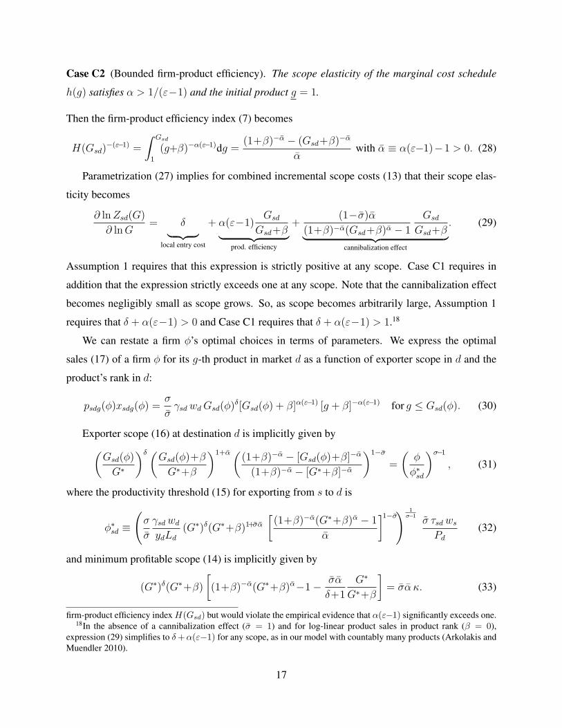
Case C2 (Bounded firm-product efficiency). The scope elasticity of the marginal cost schedule

h(g) satisfies α > 1/(ε−1) and the initial product g = 1.

Then the firm-product efficiency index (7) becomes

H(Gsd)−(ε−1) =

∫ Gsd

1

(g+β)−α(ε−1)dg =(1+β)−α − (Gsd+β)−α

αwith α ≡ α(ε−1)−1 > 0. (28)

Parametrization (27) implies for combined incremental scope costs (13) that their scope elas-

ticity becomes

∂ lnZsd(G)

∂ lnG= δ︸︷︷︸

local entry cost

+ α(ε−1)Gsd

Gsd+β︸︷︷︸prod. efficiency

+(1−σ)α

(1+β)−α(Gsd+β)α − 1

Gsd

Gsd+β︸︷︷︸cannibalization effect

. (29)

Assumption 1 requires that this expression is strictly positive at any scope. Case C1 requires in

addition that the expression strictly exceeds one at any scope. Note that the cannibalization effect

becomes negligibly small as scope grows. So, as scope becomes arbitrarily large, Assumption 1

requires that δ + α(ε−1) > 0 and Case C1 requires that δ + α(ε−1) > 1.18

We can restate a firm ϕ’s optimal choices in terms of parameters. We express the optimal

sales (17) of a firm ϕ for its g-th product in market d as a function of exporter scope in d and the

product’s rank in d:

psdg(ϕ)xsdg(ϕ) =σ

σγsdwd Gsd(ϕ)

δ[Gsd(ϕ) + β]α(ε−1) [g + β]−α(ε−1) for g ≤ Gsd(ϕ). (30)

Exporter scope (16) at destination d is implicitly given by(Gsd(ϕ)

G∗

)δ (Gsd(ϕ)+β

G∗+β

)1+α((1+β)−α − [Gsd(ϕ)+β]−α

(1+β)−α − [G∗+β]−α

)1−σ

=

(ϕ

ϕ∗sd

)σ−1

, (31)

where the productivity threshold (15) for exporting from s to d is

ϕ∗sd ≡

(σ

σ

γsd wd

ydLd

(G∗)δ(G∗+β)1+σα[(1+β)−α(G∗+β)α − 1

α

]1−σ) 1

σ−1σ τsdws

Pd

(32)

and minimum profitable scope (14) is implicitly given by

(G∗)δ(G∗+β)

[(1+β)−α(G∗+β)α−1− σα

δ+1

G∗

G∗+β

]= σα κ. (33)

firm-product efficiency index H(Gsd) but would violate the empirical evidence that α(ε−1) significantly exceeds one.18In the absence of a cannibalization effect (σ = 1) and for log-linear product sales in product rank (β = 0),

expression (29) simplifies to δ+α(ε−1) for any scope, as in our model with countably many products (Arkolakis andMuendler 2010).

17

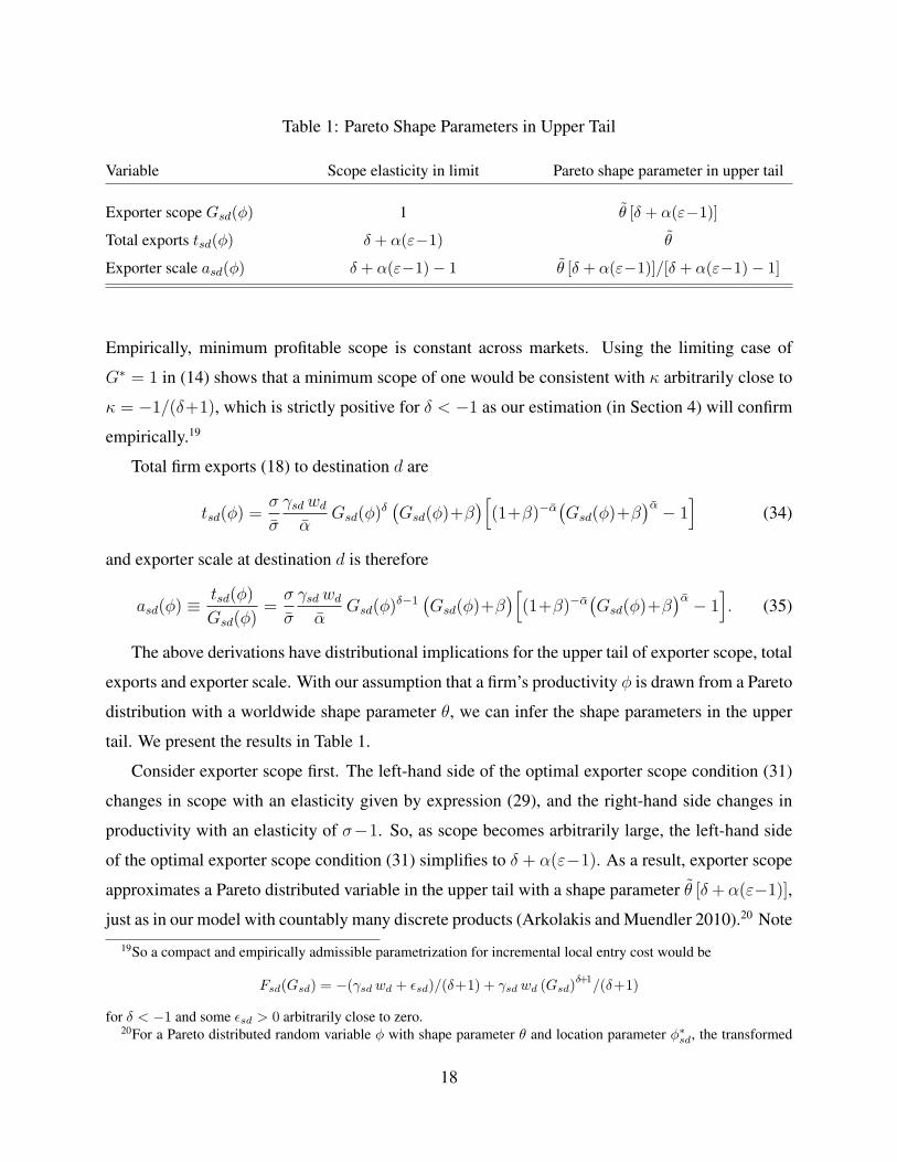
Table 1: Pareto Shape Parameters in Upper Tail

Variable Scope elasticity in limit Pareto shape parameter in upper tail

Exporter scope Gsd(ϕ) 1 θ [δ + α(ε−1)]

Total exports tsd(ϕ) δ + α(ε−1) θ

Exporter scale asd(ϕ) δ + α(ε−1)− 1 θ [δ + α(ε−1)]/[δ + α(ε−1)− 1]

Empirically, minimum profitable scope is constant across markets. Using the limiting case of

G∗ = 1 in (14) shows that a minimum scope of one would be consistent with κ arbitrarily close to

κ = −1/(δ+1), which is strictly positive for δ < −1 as our estimation (in Section 4) will confirm

empirically.19

Total firm exports (18) to destination d are

tsd(ϕ) =σ

σ

γsd wd

αGsd(ϕ)

δ(Gsd(ϕ)+β

)[(1+β)−α

(Gsd(ϕ)+β

)α − 1]

(34)

and exporter scale at destination d is therefore

asd(ϕ) ≡tsd(ϕ)

Gsd(ϕ)=

σ

σ

γsd wd

αGsd(ϕ)

δ−1(Gsd(ϕ)+β

)[(1+β)−α

(Gsd(ϕ)+β

)α − 1]. (35)

The above derivations have distributional implications for the upper tail of exporter scope, total

exports and exporter scale. With our assumption that a firm’s productivity ϕ is drawn from a Pareto

distribution with a worldwide shape parameter θ, we can infer the shape parameters in the upper

tail. We present the results in Table 1.

Consider exporter scope first. The left-hand side of the optimal exporter scope condition (31)

changes in scope with an elasticity given by expression (29), and the right-hand side changes in

productivity with an elasticity of σ−1. So, as scope becomes arbitrarily large, the left-hand side

of the optimal exporter scope condition (31) simplifies to δ + α(ε−1). As a result, exporter scope

approximates a Pareto distributed variable in the upper tail with a shape parameter θ [δ+α(ε−1)],

just as in our model with countably many discrete products (Arkolakis and Muendler 2010).20 Note19So a compact and empirically admissible parametrization for incremental local entry cost would be

Fsd(Gsd) = −(γsd wd + ϵsd)/(δ+1) + γsd wd (Gsd)δ+1

/(δ+1)

for δ < −1 and some ϵsd > 0 arbitrarily close to zero.20For a Pareto distributed random variable ϕ with shape parameter θ and location parameter ϕ∗

sd, the transformed

18

that in the absence of a cannibalization effect (σ = 1) and for log-linear product sales in product

rank (β = 0), expression (29) simplifies to δ + α(ε−1) for any scope so that exporter scope is a

Pareto distributed variable at any level.21

Now turn to total exports (34). Total exports change in exporter scope with an elasticity of

δ +G

G+β+

α

1− (1+β)α(G+β)−α

G

G+β,

which approaches δ+1+α = δ+α(ε−1) as G grows arbitrarily large. So, total exports approximate

a Pareto distributed variable in the upper tail with a shape parameter θ, which is reminiscent of

results in the Chaney (2008) and Eaton et al. (2010) models. Finally, by its definition, exporter scale

changes in exporter scope with the above elasticity less one. So, exporter scale is approximately

Pareto distributed in the upper tail with a shape parameter θ [δ + α(ε−1)]/[δ + α(ε−1)− 1].

In Appendix B we provide a comparison to the model with countably many products (Arkolakis

and Muendler 2010).

4 Estimation

Equation (30) is the basis for our estimation of the continuum model. The most important gen-

eralization compared to our estimation in Arkolakis and Muendler (2010) is that this estimation

equation accounts for a possible non-log-linearity in the relationship between firm-product sales

and product rank.22 We augment the equation by a multiplicative error term ϵsdg and estimate it in

its log form. In addition, we make local entry costs industry specific with parameters γiγsd instead

of just γsd.

random variable x = A (ϕ)B is Pareto distributed with shape θ/B and location A (ϕ∗sd)

B . To see this, apply the changeof variables theorem to ϕ(x) = (x/A)1/B and the Pareto probability density function µ(ϕ) to find that

∫ b

aµ(ϕ) dϕ =∫ x(b)

x(a)µ(ϕ(x))ϕ′(x) dx =

∫ x(b)

x(a)(θ/B) [A(ϕ∗

sd)B ]θ/B/(x)θ/B+1 dx.

21Gsd(ϕ) approaches a Pareto distribution in the upper tail because the second and third factors on the left-handside of (31) converge to a constant as Gsd(ϕ) grows. If σ approaches one, that is in the absence of a cannibalizationeffect, the third factor on the left-hand side of (31) vanishes. If β approaches zero, that is if product sales are log-linearin product rank, the first and second factor collapse to a single factor. So, in the absence of a cannibalization effectand for log-linear product sales in product rank, exporter scope is Pareto distributed at any level.

22In contrast, the presence or absence of a cannibalization effect, if products within a product line are more substi-tutable among each other than with outside products (σ < 1), is of no consequence for estimation because the resultingterm gets absorbed in the regression constant.

19

So our estimation equation becomes

ln psdg(ϕ)xisdg(ϕ) = δ lnGisd(ϕ) + α(ε−1) logGisd(ϕ) + β

− α(ε−1) log

g + β

+ ln σγi/σ + ln γsdwd + ln ϵsdg. (36)

The relationship is not log linear and we estimate equation (36) with non-linear least squares. Using

data on firm-level product sales, estimation of (36) identifies the three relevant market entry cost

parameters: the scope elasticity of incremental local entry costs δ, the scope elasticity of product

introduction costs α(ε−1), and the curvature parameter β of product introduction costs.

Firm-level sales data appear less suitable (than consumption data say) to estimate the composite

elasticity term σ ≡ (σ−1)/(ε−1), which determines the cannibalization effect. We therefore do

not attempt to quantify the cannibalization effect, which augments the costs of a wider exporter

scope.23

We use the same data on Brazilian manufacturing exporters as in Arkolakis and Muendler

(2010), which come from the universe of customs declarations for merchandize exports during

the year 2000 by any firm. From the pristine Brazilian customs records, we constructed a three-

dimensional panel of Brazilian exporters, their respective destination countries, and their export

products at the Harmonized System (HS) 6-digit level. On the product side, we restrict our data

to manufactured products only (excluding agricultural and mining products). Beyond evidence

on Brazilian manufacturing producers, we also obtain estimates for two further samples in this

paper. First, we obtain estimates for Chile, a neighboring Latin American country. We construct

a comparable three-dimensional panel of Chilean manufacturing exporters derived from the uni-

verse of customs declarations by Chilean manufacturing producers in 2000 (Alvarez, Faruq and

Lopez 2007, aggregated to the HS 6-digit level for comparison). Second, we seek evidence on lo-

cal entry costs and incremental scope costs for commercial intermediaries that ship manufactured

products.24 We report additional detail on our data and summary statistics in Appendix C. In Arko-

lakis and Muendler (2010), we present further stylized facts that robustly emerge from tabulating

and plotting our data. Our continuum model in this paper is fully consistent with those regularities.

23Evidence in Broda and Weinstein (2007) suggests that products are stronger substitutes within firms than acrossfirms so we consider a cannibalization effect with ¯σ < 1 the relevant case. Their preferred estimates for ε and σ withinand across domestic U.S. brand modules are 11.5 and 7.5.

24In 2000, our SECEX data for manufactured merchandize sold by Brazilian firms from any sector, including com-mercial intermediaries, covers 95.9 percent of Brazilian exports recorded in the World Trade Flow data (Feenstra,Lipsey, Deng, Ma and Mo 2005). Exports of manufactured merchandize shipped directly by Brazilian manufactur-

20

Table 2: Non-linear Estimates of Individual Product Sales: Continuum Casesample Any sales Sales ≥ US$100

controls Dest. Dest.&Ind. Dest. Dest.&Ind.Log Exp./prod. (1) (2) (3) (4) (5) (6)

Brazilian Producers exporting ManufacturesScope elasticity of

incr. local entry cost (δ) -1.453 -1.426 -1.332 -1.072 -1.069 -1.057(.005) (.005) (.005) (.005) (.005) (.006)

prod. efficiency (α(ε−1)) 2.985 2.965 2.951 1.872 1.945 2.079(.015) (.014) (.012) (.013) (.013) (.011)

Curvature ofprod. efficiency (β) .833 .753 .623 -.065 -.031 .014

(.025) (.023) (.019) (.017) (.017) (.015)

Obs. 162,570 162,570 162,570 141,163 141,163 141,163R2 .496 .541 .646 .370 .433 .562

Chilean Producers exporting ManufacturesScope elasticity of

incr. local entry cost (δ) -1.495 -1.394 -1.281 -1.195 -1.074 -1.009(.011) (.012) (.011) (.012) (.012) (.012)


Curvature ofprod. efficiency (β) .590 .430 .562 -.109 -.195 -.028

(.054) (.048) (.047) (.040) (.035) (.037)

Obs. 37,172 37,172 37,172 34,024 34,024 34,024R2 .419 .451 .557 .329 .375 .496

Brazilian Commercial Intermediaries exporting ManufacturesScope elasticity of

incr. local entry cost (δ) -1.281 -1.247 -1.107 -1.079 -1.015 -.913(.008) (.009) (.009) (.009) (.009) (.009)


Curvature ofprod. efficiency (β) 10.450 7.165 5.740 9.062 4.795 3.420

(.306) (.226) (.182) (.313) (.192) (.142)

Obs. 35,960 35,960 35,960 31,326 31,326 31,326R2 .489 .536 .599 .409 .469 .539

Source: Brazilian SECEX 2000, manufacturing firms as well as commercial intermediaries shipping manufacturedproducts, and Chilean customs data 2000 (Alvarez et al. 2007).Note: Products at the Harmonized-System 6-digit level. Industry fixed effects at the CNAE two-digit level for Braziland at the most frequent HS 2-digit level for Chile (highest-sale or, if tie, mode HS 2-digit product group). Constantand destination fixed effects not reported. Standard errors in parentheses. Regression equation (for g≤Gsdω):

ln psdgωxisdgω = ln γsdwd+lnσγi/σ + δ lnGisdω + α(ε−1) logGisdω+β − α(ε−1) logg + β + ln ϵisdgω,

where i indexes the industry, s the source country, d the destination, and ω the firm.

21

Table 2 presents results from estimating (36) with non-linear least squares (NLLS). To assess

robustness we estimate equation (36) with and without destination and industry fixed effects, and

separately for the subsample of firm-product sales observations of at least US$100.

Estimates for scope elasticity coefficients are robust across different specifications for the full

sales sample (columns 1 through 3). For Brazilian manufacturing producers, NLLS estimates for

the scope elasticity of incremental local entry costs δ fall in the range from −1.33 to −1.45. NLLS

estimates for the scope elasticity of product introduction costs α(ε−1) range in a narrow band

between 2.95 and 2.98. These estimates are close to the preferred OLS estimates in our companion

paper (Arkolakis and Muendler 2010, Table 3, column 4) of −1.38 for δ and 2.66 for α(σ−1).25

The NLLS estimates for Chilean manufacturing producers are close too (middle panel of Table 2),

with δ estimates ranging between −1.28 and −1.50 and α(ε−1) estimates ranging between 2.55

and 2.63. All these estimates suggest that both Case C1 and C2 are satisfied in the data. The

magnitude of the δ estimate implies that incremental local entry costs drop at an elasticity of around

−1.4 when producers introduce additional products in a market where they are present. But, as

producers introduce products further away from their core competency, firm-product efficiency

drops off even faster with an elasticity of around 2.6 in NLLS estimation at the sample mean (that

is 3.0 · 3.5/(3.5 + .6) by the elasticity of product introduction cost in equation (29) for an exporter

scope of 3.5 at the sample mean and α(ε−1) = 3.0 as well as β = .6). Combining the two

fixed scope cost components, there are net overall diseconomies of scope with a scope elasticity of

around 1.2.

The curvature parameter β in product introduction costs is statistically significantly different

from zero for the full sales sample (columns 1 through 3). This curvature parameter seems to

become relevant only because wide-scope firms introduce products with minor sales. When we

restrict the sample to products with sales of at least US$100 (columns 4 through 6), for instance,

then the curvature parameter β becomes statistically indistinguishable from zero for Brazilian man-

ufacturers in two out of three specifications (column 5 and 6), and for Chilean manufacturers in

the main specification with destination and industry fixed effects (column 6). This evidence sug-

gests that the relevant curvature in product introduction costs mainly stems from products with

ers accounts for 81.7 percent of the total manufactures exports, and manufactured merchandize shipped indirectly byBrazilian commercial intermediaries accounts for 14.2 percent.

25In Arkolakis and Muendler (2010), we restrict the relationship between firm-product sales and product rank to belog-linear, and account for residual firm-destination effects because of discrete product space.

22

minor sales. It would be misguided, however, to drop sales observations below US$100 from the

sample when estimating scope elasticities. Precisely these products with minor sales provide the

identifying information that wide-scope firms relatively easily overcome local entry costs for their

lowest-selling products, although firms must sell these minor products at fast dropping scale (in our

theory because of high marginal cost away from core competency). Estimates of scope elasticity

coefficients would not be informative in a sample with sales restricted to a minimum threshold.

The lower-most panel in Table 2 allows us to compare estimates for Brazilian commercial

intermediaries to the upper estimates for manufacturing producers. (Products in both samples

are manufactures only.) The comparison provides us with a sense of plausibility. Compared to

Brazilian manufacturing firms, Brazilian intermediaries face a less favorable scope elasticity of

incremental local entry costs δ, in a range from −1.11 to −1.28. Put differently, intermediaries do

not encounter as favorable economies of scope in local entry costs as do producers. A consistent

interpretation of this finding is that intermediaries with no production of their own do not benefit

from as rapidly declining incremental local entry costs when they introduce lower-ranked products

in a market, perhaps because they cannot count on producer reputation or brand recognition to the

same degree as a producer can. In addition, intermediaries face faster increases in product intro-

duction costs than producers, with α(ε−1) estimates ranging between 3.35 and 4.02. In addition,

intermediaries face considerably more strongly curved product introduction costs, with β estimates

between 5.7 and 10.5, compared to only between .62 and .83 for producers. One interpretation of

the latter findings is that intermediaries cannot introduce products for global sales more easily than

producers, who might also adopt products for resale, perhaps again because intermediaries cannot

rely as much on brand reputation or brand recognition. Together, these findings of more adverse

entry cost elasticities for intermediaries are consistent with the overall finding that intermediaries

account for only about a seventh of Brazilian manufacturing-product exports.

How strongly biased would a linear estimator be? For an empirical answer, we set the curvature

parameter β to zero and estimate equation (36) with OLS. Table 3 reports the results for four alter-

native specifications of fixed effects. The coefficient magnitudes are similar across specifications,

which gradually augment OLS with destination, industry and firm fixed effects. For Brazilian man-

ufacturing producers, log-linear estimates for the scope elasticity of incremental local entry costs

δ fall in the range from −1.17 to −1.56 (embracing the NLLS estimates). Log-linear estimates

for the scope elasticity of product introduction costs α(ε−1) range in a band between 2.51 and

23

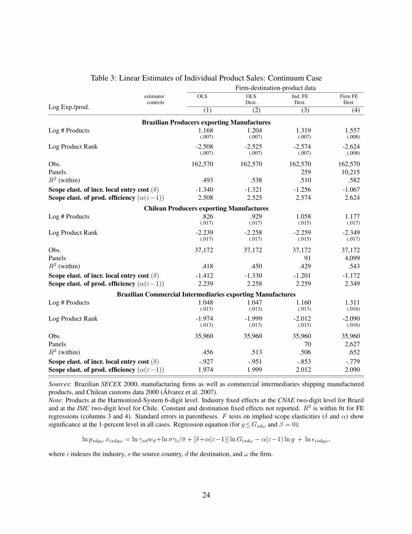
Table 3: Linear Estimates of Individual Product Sales: Continuum CaseFirm-destination-product data

estimator OLS OLS Ind. FE Firm FEcontrols Dest. Dest. Dest.

Log Exp./prod. (1) (2) (3) (4)

Brazilian Producers exporting ManufacturesLog # Products 1.168 1.204 1.319 1.557

(.007) (.007) (.007) (.008)

Log Product Rank -2.508 -2.525 -2.574 -2.624(.007) (.007) (.007) (.008)

Obs. 162,570 162,570 162,570 162,570Panels 259 10,215R2 (within) .493 .538 .510 .582Scope elast. of incr. local entry cost (δ) -1.340 -1.321 -1.256 -1.067Scope elast. of prod. efficiency (α(ε−1)) 2.508 2.525 2.574 2.624

Chilean Producers exporting ManufacturesLog # Products .826 .929 1.058 1.177

(.017) (.017) (.015) (.017)

Log Product Rank -2.239 -2.258 -2.259 -2.349(.017) (.017) (.015) (.017)

Obs. 37,172 37,172 37,172 37,172Panels 91 4,099R2 (within) .418 .450 .429 .543Scope elast. of incr. local entry cost (δ) -1.412 -1.330 -1.201 -1.172Scope elast. of prod. efficiency (α(ε−1)) 2.239 2.258 2.259 2.349

Brazilian Commercial Intermediaries exporting ManufacturesLog # Products 1.048 1.047 1.160 1.311

(.013) (.013) (.013) (.016)

Log Product Rank -1.974 -1.999 -2.012 -2.090(.013) (.013) (.013) (.016)

Obs. 35,960 35,960 35,960 35,960Panels 70 2,627R2 (within) .456 .513 .506 .652Scope elast. of incr. local entry cost (δ) -.927 -.951 -.853 -.779Scope elast. of prod. efficiency (α(ε−1)) 1.974 1.999 2.012 2.090

Sources: Brazilian SECEX 2000, manufacturing firms as well as commercial intermediaries shipping manufacturedproducts, and Chilean customs data 2000 (Alvarez et al. 2007).Note: Products at the Harmonized-System 6-digit level. Industry fixed effects at the CNAE two-digit level for Braziland at the ISIC two-digit level for Chile. Constant and destination fixed effects not reported. R2 is within fit for FEregressions (columns 3 and 4). Standard errors in parentheses. F tests on implied scope elasticities (δ and α) showsignificance at the 1-percent level in all cases. Regression equation (for g≤Gsdω and β = 0):

ln psdgω xisdgω = ln γsdwd+lnσγi/σ + [δ+α(ε−1)] lnGisdω − α(ε−1) ln g + ln ϵisdgω,

where i indexes the industry, s the source country, d the destination, and ω the firm.

24

2.62 (somewhat below the NLLS estimates). These estimates too are close to the preferred OLS

estimates in our companion paper (Arkolakis and Muendler 2010, Table 3, column 4) of −1.38 for

δ and 2.66 for α(σ−1).

Their similarity notwithstanding, the variation in coefficient magnitudes across specifications

confirms an expected underlying bias from log-linear estimation. For a zero curvature parameter

β, the theoretically most adequate specification contains industry and destination fixed effects (col-

umn 3). We know from NLLS estimation, however, that the curvature parameter is non-zero. We

expect the omission of the non-linear curvature component to introduce a negative bias into OLS

estimation. The reason is that the curvature parameter β matters most for narrow-scope firms with

low productivity, because their exports per product are pushed relatively higher (β > 0) than prod-

uct sales by the mean firm, while the curvature parameter matters little for wide-scope firms with

high productivity, because their scope is large compared to β so that their exports per product are

pushed up less than product sales by the mean firm. A firm fixed effect is a simple non-parametric

way to control for omitted firm characteristics such as unobserved productivity.26 Indeed, inclusion

of a firm fixed effect raises the regression coefficient on the number of products in confirmation of

a negative bias (comparing columns 3 and 4).

In economic terms, however, the bias from omitting the non-linear curvature term is small for

manufacturing producers. In the Brazilian producer sample, the scope elasticity of incremental

local entry costs δ is estimated to be −1.26 under OLS (column 3) instead of −1.33 under NLLS

(Table 2 column 3), and the scope elasticity of product introduction costs α(ε−1) is estimated as

2.57 under OLS instead of 2.95 under NLLS. In the Chilean producer sample, the scope elasticity

of incremental local entry costs δ is estimated to be −1.20 under OLS instead of −1.28 under

NLLS, and the scope elasticity of product introduction costs α(ε−1) is estimated as 2.26 under

OLS instead of 2.63 under NLLS.

These small differences justify our restriction to log-linearity of firm-product sales and OLS

estimation in our companion paper (Arkolakis and Muendler 2010). For commercial intermedi-

aries, however, the non-log-linearity in product introduction costs matters considerably for product

introduction cost estimation. In the Brazilian intermediary sample, the scope elasticity of incre-

mental local entry costs δ is estimated to be −1.16 under OLS and still close to the estimate of

26Our model with countably many products (Arkolakis and Muendler 2010) also calls for a firm fixed effect tocontrol for incrementally changing exports per product as a firm becomes more productive, while its exporter scoperemains unchanged between discrete thresholds.

25

−1.11 under NLLS, but the scope elasticity of product introduction costs α(ε−1) is estimated as

only 2.01 under OLS instead of 3.35 under NLLS, a downward bias of forty percent under OLS.

5 Conclusion

Market entry costs are a crucial component in recent trade theory. Combined with firm hetero-

geneity, fixed market entry costs can provide novel predictions of exporter behavior and aggregate

exports. This companion paper to Arkolakis and Muendler (2010) presents a generalized model of

multi-product exporters that allows for two additional components of market entry costs. In contin-

uous product space, we consider a cannibalization effect by which additional products reduce the

sales of a firm’s infra-marginal products, and we allow for product sales that drop off faster than

log linearly as a firm adds products that sell for ever smaller amounts. The model preserves main

predictions of prior heterogeneous-firm models of trade, such as a single elasticity of exporting and

a power-law distribution of exports in the upper tail. Our model generates in addition estimable

equations to identify several relevant market entry cost parameters.

Our evidence suggests that there is relevant curvature in product introduction costs, and that

this curvature mainly stems from products with minor sales. The existence of products with minor

sales is, in turn, consistent with the main mechanism of our theory: highly productive wide-scope

firms overcome local entry costs for their lowest-selling products relatively easily but they face

fast increasing marginal production costs away from core competency. For Brazilian manufac-

turing producers, our non-linear least squares estimates confirm the more restrictive ones from

earlier work. The estimates continue to be consistent with the hypothesis that producers encounter

economies of scope in fixed local entry costs but even stronger diseconomies of scope in product

introduction costs so that the firms face overall diseconomies of scope in every destination market.

26

Appendix

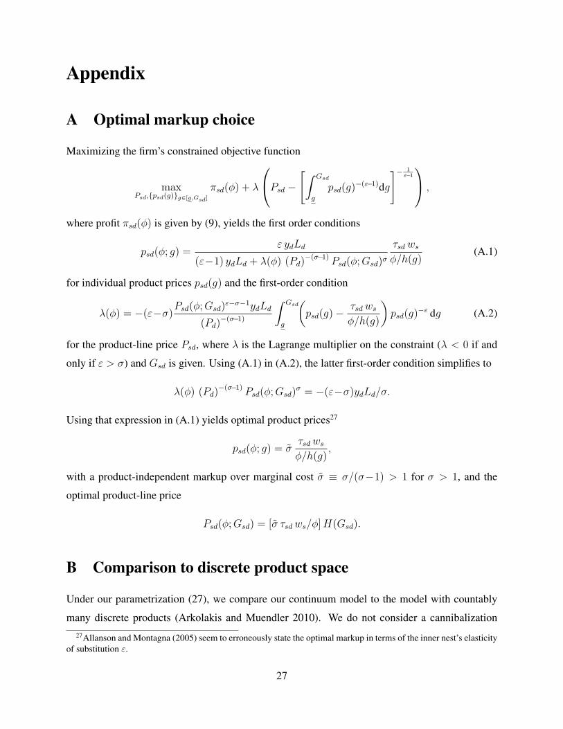
A Optimal markup choice

Maximizing the firm’s constrained objective function

maxPsd,psd(g)g∈[g,Gsd]

πsd(ϕ) + λ

Psd −

[∫ Gsd

g

psd(g)−(ε−1)dg

]− 1ε−1 ,

where profit πsd(ϕ) is given by (9), yields the first order conditions

psd(ϕ; g) =ε ydLd

(ε−1) ydLd + λ(ϕ) (Pd)−(σ−1) Psd(ϕ;Gsd)σ

τsd ws

ϕ/h(g)(A.1)

for individual product prices psd(g) and the first-order condition

λ(ϕ) = −(ε−σ)Psd(ϕ;Gsd)

ε−σ−1ydLd

(Pd)−(σ−1)

∫ Gsd

g

(psd(g)−

τsdws

ϕ/h(g)

)psd(g)

−ε dg (A.2)

for the product-line price Psd, where λ is the Lagrange multiplier on the constraint (λ < 0 if and

only if ε > σ) and Gsd is given. Using (A.1) in (A.2), the latter first-order condition simplifies to

λ(ϕ) (Pd)−(σ−1) Psd(ϕ;Gsd)

σ = −(ε−σ)ydLd/σ.

Using that expression in (A.1) yields optimal product prices27

psd(ϕ; g) = στsd ws

ϕ/h(g),

with a product-independent markup over marginal cost σ ≡ σ/(σ−1) > 1 for σ > 1, and the

optimal product-line price

Psd(ϕ;Gsd) = [σ τsdws/ϕ]H(Gsd).

B Comparison to discrete product space

Under our parametrization (27), we compare our continuum model to the model with countably

many discrete products (Arkolakis and Muendler 2010). We do not consider a cannibalization27Allanson and Montagna (2005) seem to erroneously state the optimal markup in terms of the inner nest’s elasticity

of substitution ε.

27

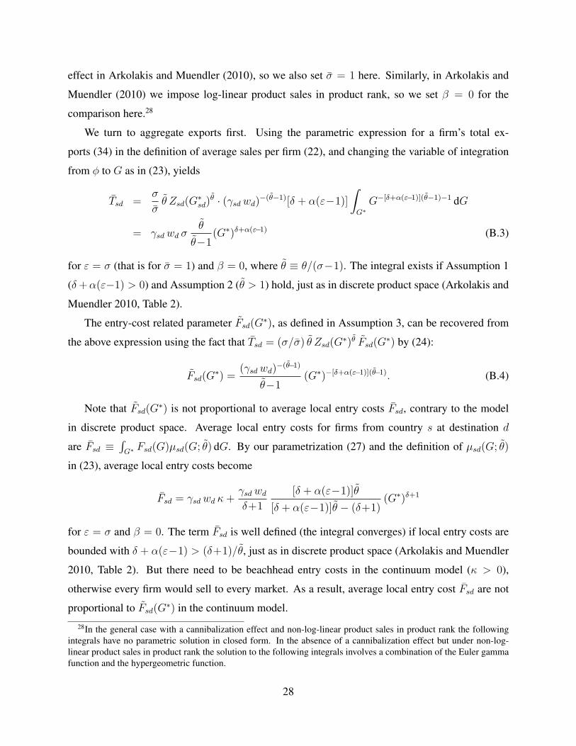
effect in Arkolakis and Muendler (2010), so we also set σ = 1 here. Similarly, in Arkolakis and

Muendler (2010) we impose log-linear product sales in product rank, so we set β = 0 for the

comparison here.28

We turn to aggregate exports first. Using the parametric expression for a firm’s total ex-

ports (34) in the definition of average sales per firm (22), and changing the variable of integration

from ϕ to G as in (23), yields

Tsd =σ

σθ Zsd(G

∗sd)

θ · (γsdwd)−(θ−1)[δ + α(ε−1)]

∫G∗

G−[δ+α(ε−1)](θ−1)−1 dG

= γsd wd σθ

θ−1(G∗)δ+α(ε−1) (B.3)

for ε = σ (that is for σ = 1) and β = 0, where θ ≡ θ/(σ−1). The integral exists if Assumption 1

(δ+α(ε−1) > 0) and Assumption 2 (θ > 1) hold, just as in discrete product space (Arkolakis and

Muendler 2010, Table 2).

The entry-cost related parameter Fsd(G∗), as defined in Assumption 3, can be recovered from

the above expression using the fact that Tsd = (σ/σ) θ Zsd(G∗)θ Fsd(G

∗) by (24):

Fsd(G∗) =

(γsdwd)−(θ−1)

θ−1(G∗)−[δ+α(ε−1)](θ−1). (B.4)

Note that Fsd(G∗) is not proportional to average local entry costs Fsd, contrary to the model

in discrete product space. Average local entry costs for firms from country s at destination d

are Fsd ≡∫G∗ Fsd(G)µsd(G; θ) dG. By our parametrization (27) and the definition of µsd(G; θ)

in (23), average local entry costs become

Fsd = γsdwd κ+γsd wd

δ+1

[δ + α(ε−1)]θ

[δ + α(ε−1)]θ − (δ+1)(G∗)δ+1

for ε = σ and β = 0. The term Fsd is well defined (the integral converges) if local entry costs are

bounded with δ + α(ε−1) > (δ+1)/θ, just as in discrete product space (Arkolakis and Muendler

2010, Table 2). But there need to be beachhead entry costs in the continuum model (κ > 0),

otherwise every firm would sell to every market. As a result, average local entry cost Fsd are not

proportional to Fsd(G∗) in the continuum model.

28In the general case with a cannibalization effect and non-log-linear product sales in product rank the followingintegrals have no parametric solution in closed form. In the absence of a cannibalization effect but under non-log-linear product sales in product rank the solution to the following integrals involves a combination of the Euler gammafunction and the hypergeometric function.

28

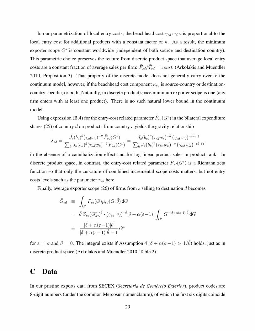
In our parametrization of local entry costs, the beachhead cost γsdwd κ is proportional to the

local entry cost for additional products with a constant factor of κ. As a result, the minimum

exporter scope G∗ is constant worldwide (independent of both source and destination country).

This parametric choice preserves the feature from discrete product space that average local entry

costs are a constant fraction of average sales per firm: Fsd/Tsd = const. (Arkolakis and Muendler

2010, Proposition 3). That property of the discrete model does not generally carry over to the

continuum model, however, if the beachhead cost component κsd is source-country or destination-

country specific, or both. Naturally, in discrete product space minimum exporter scope is one (any

firm enters with at least one product). There is no such natural lower bound in the continuum

model.

Using expression (B.4) for the entry-cost related parameter Fsd(G∗) in the bilateral expenditure

shares (25) of country d on products from country s yields the gravity relationship

λsd =Js(bs)

θ(τsdws)−θ Fsd(G

∗)∑k Jk(bk)

θ(τkdwk)−θ Fkd(G∗)=

Js(bs)θ(τsdws)

−θ (γsd wd)−(θ−1)∑

k Jk(bk)θ(τkdwk)−θ (γkd wd)−(θ−1)

in the absence of a cannibalization effect and for log-linear product sales in product rank. In

discrete product space, in contrast, the entry-cost related parameter Fsd(G∗) is a Riemann zeta

function so that only the curvature of combined incremental scope costs matters, but not entry

costs levels such as the parameter γsd here.

Finally, average exporter scope (26) of firms from s selling to destination d becomes

Gsd ≡∫G∗

Fsd(G)µsd(G; θ) dG

= θ Zsd(G∗sd)

θ · (γsd wd)−θ[δ + α(ε−1)]

∫G∗

G−[δ+α(ε−1)]θ dG

=[δ + α(ε−1)]θ

[δ + α(ε−1)]θ − 1G∗

for ε = σ and β = 0. The integral exists if Assumption 4 (δ + α(σ−1) > 1/θ) holds, just as in

discrete product space (Arkolakis and Muendler 2010, Table 2).

C Data

In our pristine exports data from SECEX (Secretaria de Comercio Exterior), product codes are

8-digit numbers (under the common Mercosur nomenclature), of which the first six digits coincide

29

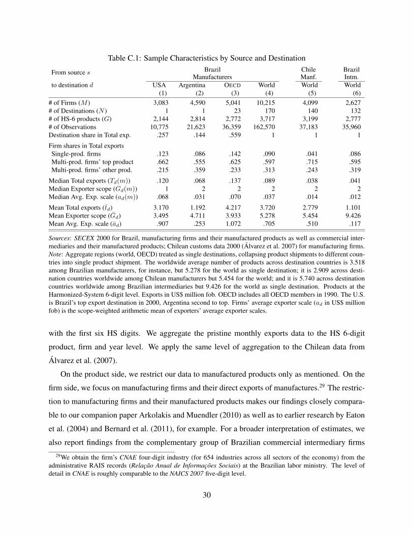
Table C.1: Sample Characteristics by Source and DestinationBrazil Chile BrazilFrom source s

Manufacturers Manf. Intm.to destination d USA Argentina OECD World World World

(1) (2) (3) (4) (5) (6)# of Firms (M ) 3,083 4,590 5,041 10,215 4,099 2,627# of Destinations (N ) 1 1 23 170 140 132# of HS-6 products (G) 2,144 2,814 2,772 3,717 3,199 2,777# of Observations 10,775 21,623 36,359 162,570 37,183 35,960Destination share in Total exp. .257 .144 .559 1 1 1

Firm shares in Total exportsSingle-prod. firms .123 .086 .142 .090 .041 .086Multi-prod. firms’ top product .662 .555 .625 .597 .715 .595Multi-prod. firms’ other prod. .215 .359 .233 .313 .243 .319

Median Total exports (Td(m)) .120 .068 .137 .089 .038 .041Median Exporter scope (Gd(m)) 1 2 2 2 2 2Median Avg. Exp. scale (ad(m)) .068 .031 .070 .037 .014 .012

Mean Total exports (td) 3.170 1.192 4.217 3.720 2.779 1.101Mean Exporter scope (Gd) 3.495 4.711 3.933 5.278 5.454 9.426Mean Avg. Exp. scale (ad) .907 .253 1.072 .705 .510 .117

Sources: SECEX 2000 for Brazil, manufacturing firms and their manufactured products as well as commercial inter-mediaries and their manufactured products; Chilean customs data 2000 (Alvarez et al. 2007) for manufacturing firms.Note: Aggregate regions (world, OECD) treated as single destinations, collapsing product shipments to different coun-tries into single product shipment. The worldwide average number of products across destination countries is 3.518among Brazilian manufacturers, for instance, but 5.278 for the world as single destination; it is 2.909 across desti-nation countries worldwide among Chilean manufacturers but 5.454 for the world; and it is 5.740 across destinationcountries worldwide among Brazilian intermediaries but 9.426 for the world as single destination. Products at theHarmonized-System 6-digit level. Exports in US$ million fob. OECD includes all OECD members in 1990. The U.S.is Brazil’s top export destination in 2000, Argentina second to top. Firms’ average exporter scale (ad in US$ millionfob) is the scope-weighted arithmetic mean of exporters’ average exporter scales.

with the first six HS digits. We aggregate the pristine monthly exports data to the HS 6-digit

product, firm and year level. We apply the same level of aggregation to the Chilean data from

Alvarez et al. (2007).

On the product side, we restrict our data to manufactured products only as mentioned. On the

firm side, we focus on manufacturing firms and their direct exports of manufactures.29 The restric-

tion to manufacturing firms and their manufactured products makes our findings closely compara-

ble to our companion paper Arkolakis and Muendler (2010) as well as to earlier research by Eaton

et al. (2004) and Bernard et al. (2011), for example. For a broader interpretation of estimates, we

also report findings from the complementary group of Brazilian commercial intermediary firms

29We obtain the firm’s CNAE four-digit industry (for 654 industries across all sectors of the economy) from theadministrative RAIS records (Relacao Anual de Informacoes Sociais) at the Brazilian labor ministry. The level ofdetail in CNAE is roughly comparable to the NAICS 2007 five-digit level.

30

and their exports of manufactures. We remove export records with zero value from the Brazilian

data, which include shipments of commercial samples but also potential reporting errors, and lose

408 of initially 162,978 exporter-destination-product observations. Our results on exporter scope

do not materially change when including or excluding zero-shipment products from the product

count. There are no reported shipments with zero value in the Chilean data.

Our Brazilian manufacturer sample includes 10,215 firms with shipments of 3,717 manufac-

turing products at the 6-digit Harmonized System level to 170 foreign destinations, and a total of

162,570 exporter-destination-product observations. The Chilean manufacturer sample is consid-

erably smaller; it has 4,099 firms with shipments of 3,199 manufacturing products at the 6-digit

Harmonized System level to 140 foreign destinations, and a total of 37,183 exporter-destination-

product observations. Our Brazilian intermediary sample includes 2,627 firms in the commercial

sector with shipments of 2,777 manufacturing products at the 6-digit Harmonized System level to

132 foreign markets, and a total of 35,960 exporter-destination-product observations. Exporters

shipping multiple products dominate. They ship more than ninety percent of all exports both

from Brazil and Chile, and their single top-selling products account for almost sixty percent of all

Brazilian exports and more than seventy percent of all Chilean exports.

To analyze export behavior, we decompose a firm ϕ’s total exports tdϕ from Brazil or Chile to

destination market d into the firm’s number of products sold at d (the exporter scope) Gdϕ and the

firm’s average sales per export product in d (the average exporter scale) adϕ ≡ tdϕ/Gdϕ:

tdϕ =∑Gdϕ

g=1 pdgϕxdgϕ = Gdϕ adϕ,

where pdgϕ is the price of product g and xdgϕ its export quantity. To calculate summary medians and

means of these variables for regional aggregates and the world as a whole in Table C.1 (columns 3

to 6), we treat the aggregate as if it were a single destination and collapse all product shipments

to different countries into a single product shipment. For estimation in the text, in contrast, we

analyze these variables country by country.

The median exporter is a relatively small exporter, with sales to the rest of the world totalling

around US$ 90,000 from Brazil (column 4) and US$ 40,000 from Chile (column 5). The mean

Brazilian (Chilean) exporter, in contrast, sells around US$ 3.7 (2.8) million abroad, more than

40 (70) times as much as the median manufacturer. Exporter scope and average exporter scale

exhibit similarly stark differences between mean and median. The median Brazilian manufacturer

sells two products worldwide, but the mean scope per firm is 5.3 products. The median Brazilian

31

manufacturer has sales of around US$ 40,000 per product, but the mean exporter scale per exporter

is US$ 700,000, or around 20 times as high as that for the median firm.30

The importance of the top-selling product at multi-product exporters and the mean-median ra-

tios repeat across destinations. To investigate the robustness across countries, we select Brazil’s top

two export destinations (United States and Argentina), as well as the OECD aggregate. Our theory

emphasizes the importance of exporting behavior within destinations. Within single countries, the

mean manufacturer’s exports exceed the median manufacturer’s exports by similarly large factors

as in the aggregate, between 14 (in Argentina, column 2) and 26 (in the United States, column 1).

In the OECD aggregate (column 3), exports of the mean firm exceed the exports of the median

firm by a factor of about 30. Interestingly, the same mean-median ratio of about 30 prevails in the

non-OECD aggregate (not reported).

We also investigate Brazil’s commercial intermediaries and their manufacturing-product ship-

ments. The shares of single- and multi-product firms are strikingly similar for intermediaries sell-

ing manufactured products (column 6) and the manufacturers shipping directly (column 4). The

mean-median ratios vary more, however. While the mean Brazilian manufacturer sells more than

40 times as much as the median manufacturer, the mean Brazilian commercial intermediary sells

only around 30 times as much as the median intermediary. This differences between Brazilian

manufacturers and intermediaries is due to a smaller mean-median ratio for average exporter scale

at intermediaries than at manufacturers (10 times versus 20 times), whereas the mean intermediary

sells more than nine products worldwide compared to the mean manufacturer with only five.

30 The means in Table C.1 are calculated as follows. A source country’s total exports Td are decomposed into Td =Md Gd ad, where Md is the number of exporters to destination d, Gd ≡

∑Md

ϕ=1 Gd(ϕ)/Md is the exporters’ mean ex-porter scope, and ad ≡ td/Gd is the average exporter scale (the products’ mean sales at those firms). Equivalently, adis the weighted arithmetic mean of ad(ϕ) over all ϕ, with weights Gd(ϕ): ad =

∑Md

ϕ=1 Gd(ϕ) ad(ϕ)/[∑Md

ϕ=1 Gd(ϕ)] =

td/Gd. As the decomposition shows, scope weighting is necessary for the mean scope and the mean exporter scale toyield total exports when multiplied.

32

ReferencesAllanson, Paul and Catia Montagna, “Multiproduct Firms and Market Structure: An Explorative Appli-

cation to the Product Life Cycle,” International Journal of Industrial Organization, September 2005, 23(7-8), 587–597.

Alvarez, Roberto, Hasan Faruq, and Ricardo A. Lopez, “New Products in Export Markets: Learningfrom Experience and Learning from Others,” August 2007. Indiana University, Bloomington, unpublishedmanuscript.

Arkolakis, Costas and Marc-Andreas Muendler, “The Extensive Margin of Exporting Products: A Firm-level Analysis,” NBER Working Paper, December 2010, 16641.

Atkeson, Andrew and Ariel T. Burstein, “Pricing-to-Market, Trade Costs, and International RelativePrices,” American Economic Review, December 2008, 98 (5), 1998–2031.

Bernard, Andrew B., Stephen J. Redding, and Peter K. Schott, “Multi-product Firms and Trade Liber-alization,” Quarterly Journal of Economics, 2011. advance access July 19, 2011.

Broda, Christian and David E. Weinstein, “Product Creation and Destruction: Evidence and Price Impli-cations,” NBER Working Paper, 2007, 13041.

Chaney, Thomas, “Distorted Gravity: The Intensive and Extensive Margins of International Trade,” Amer-ican Economic Review, September 2008, 98 (4), 1707–21.

Eaton, Jonathan and Samuel Kortum, “Technology, Geography, and Trade,” Econometrica, September2002, 70 (5), 1741–79.

, , and Francis Kramarz, “Dissecting Trade: Firms, Industries, and Export Destinations,” AmericanEconomic Review: Papers and Proceedings, May 2004, 94 (2), 150–54.

, , and , “An Anatomy of International Trade: Evidence from French Firms,” February 2010. Uni-versity of Chicago, unpublished manuscript.

Eckel, Carsten and J. Peter Neary, “Multi-Product Firms and Flexible Manufacturing in the Global Econ-omy,” Review of Economic Studies, January 2010, 77 (1), 188–217.

Feenstra, Robert C. and Hong Ma, “Optimal Choice of Product Scope for Multiproduct Firms under Mo-nopolistic Competition,” in Elhanan Helpman, Dalia Marin, and Thierry Verdier, eds., The Organizationof Firms in a Global Economy, Cambridge, Mass.: Harvard University Press, November 2008, chapter 6,pp. 173–199.

, Robert E. Lipsey, Haiyan Deng, Alyson C. Ma, and Hengyong Mo, “World Trade Flows: 1962-2000,” NBER Working Paper, January 2005, 11040.

Helpman, Elhanan, Marc J. Melitz, and Stephen R. Yeaple, “Export versus FDI with HeterogeneousFirms,” American Economic Review, March 2004, 94 (1), 300–316.

Krugman, Paul R., “Scale Economies, Product Differentiation, and the Pattern of Trade,” American Eco-nomic Review, 1980, 70 (5), 950–59.

33

Mayer, Thierry, Marc J. Melitz, and Gianmarco I.P. Ottaviano, “Market Size, Competition, and theProduct Mix of Exporters,” NBER Working Paper, April 2011, 16959.

Melitz, Marc J., “The Impact of Trade on Intra-Industry Reallocations and Aggregate Industry Productiv-ity,” Econometrica, November 2003, 71 (6), 1695–1725.

Nocke, Volker and Stephen R. Yeaple, “Globalization and Endogenous Firm Scope,” NBER WorkingPaper, June 2006, 12322.

34

the extensive margin of exporting products: the continuum...

Documents