The expanding universe: an introduction

Lecture at the WE Heraeus Summer School“Astronomy from Four Perspectives”, Heidelberg

Markus Possel, Haus der Astronomie

28 August 2017

Contents

1 Introduction 3

2 Length scales and the realm of cosmology 4

3 General relativity 63.1 Equivalence principle . . . . . . . . . . . . . . . . . . . . . . . . . 63.2 Tidal forces and the limits of the equivalence principle . . . . . . 83.3 The equivalence principle, reformulated . . . . . . . . . . . . . . 103.4 Tidal deformations and attraction . . . . . . . . . . . . . . . . . 103.5 Newtonian limit and Einstein’s equation(s) . . . . . . . . . . . . 133.6 What we need from general relativity . . . . . . . . . . . . . . . . 15

4 A homogeneous, isotropic, expanding universe 154.1 What can change in a homogeneous universe? . . . . . . . . . . . 184.2 Scale-factor expansion . . . . . . . . . . . . . . . . . . . . . . . . 204.3 Cosmic time t and proper distance d . . . . . . . . . . . . . . . . 22

5 The Hubble relation 235.1 Free-falling galaxies and the Doppler effect . . . . . . . . . . . . 255.2 Measuring astronomical distances . . . . . . . . . . . . . . . . . . 275.3 Measuring the Hubble constant . . . . . . . . . . . . . . . . . . . 305.4 Approximating a(t) . . . . . . . . . . . . . . . . . . . . . . . . . . 33

6 Consequences of scale-factor expansion 346.1 Diluting the universe . . . . . . . . . . . . . . . . . . . . . . . . . 356.2 Redshifting photons . . . . . . . . . . . . . . . . . . . . . . . . . 386.3 Light propagation in an expanding universe . . . . . . . . . . . . 406.4 Cosmological redshift revisited . . . . . . . . . . . . . . . . . . . 436.5 Redshift drift . . . . . . . . . . . . . . . . . . . . . . . . . . . . . 456.6 The geometry of space . . . . . . . . . . . . . . . . . . . . . . . . 466.7 Luminosity, apparent brightness, and distance . . . . . . . . . . . 496.8 Luminosity distance and distance moduli . . . . . . . . . . . . . 50

1

arX

iv:1

712.

1031

5v1

[gr

-qc]

29

Dec

201

7

7 Dynamics: how a(t) changes over (cosmic) time 517.1 Friedmann’s equations . . . . . . . . . . . . . . . . . . . . . . . . 527.2 Filling the universe with different kinds of matter . . . . . . . . . 557.3 Dimensionless Friedmann equation and light-travel distance . . . 567.4 Densities and geometry . . . . . . . . . . . . . . . . . . . . . . . 587.5 Different eras of cosmic history; the Big Bang singularity . . . . 607.6 Expansion and collapse . . . . . . . . . . . . . . . . . . . . . . . 647.7 Explicit solutions . . . . . . . . . . . . . . . . . . . . . . . . . . . 65

8 Consequences of cosmic evolution 698.1 Horizons . . . . . . . . . . . . . . . . . . . . . . . . . . . . . . . . 698.2 Do galaxies, humans, atoms expand? . . . . . . . . . . . . . . . . 708.3 The fate of our own universe . . . . . . . . . . . . . . . . . . . . 778.4 The generalized redshift-distance relation . . . . . . . . . . . . . 798.5 Comparing distances . . . . . . . . . . . . . . . . . . . . . . . . . 81

9 The Redshift-distance diagram revisited 83

10 Conclusions 84

11 Bibliography 86

Index 93

A Fitting the supernova data 97

B What we need from special relativity 98B.1 Inertial reference frames . . . . . . . . . . . . . . . . . . . . . . . 98B.2 Relativity principle and constant light speed . . . . . . . . . . . . 99B.3 Transformations . . . . . . . . . . . . . . . . . . . . . . . . . . . 100B.4 Time dilation . . . . . . . . . . . . . . . . . . . . . . . . . . . . . 101B.5 Doppler effect . . . . . . . . . . . . . . . . . . . . . . . . . . . . . 102B.6 E = mc2 . . . . . . . . . . . . . . . . . . . . . . . . . . . . . . . . 104B.7 Energy, momentum, and pressure . . . . . . . . . . . . . . . . . . 106

Acknowledgements 107

2

1 Introduction

Modern cosmology is based on general relativity. Teaching general relativity isa challenge — if you go all the way, you will need mathematical concepts soadvanced that they are not even included in the usual mathematics courses forstudents of physics. Typical graduate-level lectures on general relativity thusneed to include sections introducing the necessary mathematical formalism,notably concepts from differential geometry.

For introducing general relativity to undergraduates, or even in a high schoolsetting, simplifications are necessary, leading to the central question: in generalrelativity, how far can you go without the full formalism? In this lecture, we willask this question in the context of cosmology: Which aspects of the expandinguniverse, of the modern cosmological models, can you understand without usingthe formalism of general relativity?

On the simplest level, this brings us to the various models commonly usedto explain cosmic expansion – the expanding rubber balloon, the linear rubberband as a one-dimensional universe, and the raisin cake (Eddington 1930, Lotze1995, Price and Grover 2001, Fraknoi 1995, Strauss 2016). Used judiciously,these models can convey a basic understanding of what it means for a universeto be expanding. The main focus of this lecture is on quantitative results,though: How many of the calculations of standard cosmology can we reproducewithout employing the formalism of general relativity?

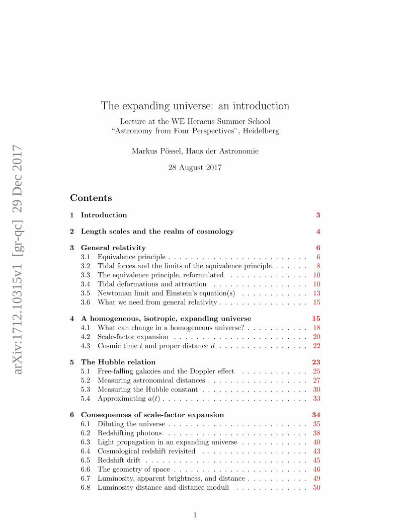
As it turns out, in the context of cosmology, the basic tenets of generalrelativity can take you quite a long way. Our goal in these lecture notes will be tounderstand the basic predictions of the Friedmann-Lemaıtre-Robertson-Walkermodels, expanding homogeneous universes that form the backbone of the BigBang models of modern cosmology, along these lines. More specifically, ourgoal will be to understand one of the most important links between cosmologicalmodels and astronomical observations: the generalized Hubble diagram, linkingthe distances of certain standard candles (that is, objects of known brightness)and their redshifts. Figure 1 shows an example (namely figure 4 in Suzuki etal. 2012).

How come that all these sources lie along this particular curve? How do wederive the curve’s shape, and how is it linked to fundamental properties of theuniverse?

The following notes have grown out of a lecture with the title “Introducingthe expanding universe without using the concept of a spacetime metric,” whichI held on 28 August 2017 at Haus der Astronomie, at our WE Heraeus Sum-mer School “Astronomy from four perspectives,” a summer school for teachers,students training to be teachers, astronomers and astronomy students fromHeidelberg, Padova, Jena, and Florence. This year’s theme was “The DarkUniverse,” an exploration of dark matter and dark energy. An edited versionof the lecture can be found on YouTube at

http://youtu.be/gA-0C-88WbE

The aim of the lecture was to give a basic overview of modern cosmologicalmodels, in order to prepare our participants for more specialized lectures and

3

15

0.0 0.2 0.4 0.6 0.8 1.0 1.2 1.4

Redshift

32

34

36

38

40

42

44

46D

ista

nce

Modulu

s

Hamuy et al. (1996)Krisciunas et al. (2005)Riess et al. (1999)Jha et al. (2006)Kowalski et al. (2008) (SCP)Hicken et al. (2009)Contreras et al. (2010) Holtzman et al. (2009)

Riess et al. (1998) + HZTPerlmutter et al. (1999) (SCP)Barris et al. (2004)Amanullah et al. (2008) (SCP)Knop et al. (2003) (SCP)Astier et al. (2006)Miknaitis et al. (2007)

Tonry et al. (2003)Riess et al. (2007)Amanullah et al. (2010) (SCP)Cluster Search (SCP)

Figure 4. Hubble diagram for the Union2.1 compilation. The solid linerepresents the best-fit cosmology for a flatΛCDM Universe for supernovae alone.SN SCP06U4 falls outside the allowedx1 range and is excluded from the current analysis. When fit witha newer version of SALT2, this supernova passes thecut and would be included, so we plot it on the Hubble diagram,but with a red triangle symbol.

Table 4Assumed instrumental uncertainties for SNe in this paper.

Source Band Uncertainty Reference

HST WFPC2 0.02 Heyer et al. (2004)ACS F850LP 0.01 Bohlin (2007)ACS F775W 0.01ACS F606W 0.01ACS F850LP 94A Bohlin (2007)ACS F775W 57AACS F606W 27ANICMOS J 0.024 Ripoche et. al. (in prep), Section 3.2.1NICMOS H 0.06 de Jong et al. (2006)

SNLS g, r, i 0.01 Astier et al. (2006)z 0.03

ESSENCE R, I 0.014 Wood-Vasey et al. (2007)SDSS u 0.014 Kessler et al. (2009)

g, r, i 0.009z 0.010

SCP: Amanullah et al. (2010) R, I 0.03 Amanullah et al. (2010)J 0.02

Other U -band 0.04 Hicken et al. (2009a)Other Band 0.02 Hicken et al. (2009a)

Figure 1: Distance moduli plotted against redshift for various standard candles. Figure 4 inSuzuki et al. 2012, available at http://www-supernova.lbl.gov/

tutorials. The lecture’s goal of making cosmology understandable without in-troducing the underlying formalism was motivated both by the diverse back-grounds of the listeners and by the summer school’s underlying goal of makingmodern astronomical research accessible to high school students.

On the part of the reader, I assume familiarity with basic classical me-chanics, including Newton’s law of gravity, and the basics of special relativity;in order to make the text more accessible, the content we need from specialrelativity is summarised in appendix B.

2 Length scales and the realm of cosmology

Seen naively, cosmology is the most ambitious science. We aim to understandthe universe as a whole! The universe, as everyday experience shows, is rathercomplex, with many different interesting scales, comprising everything frominsects via humans, city-scale structures, moons, planets, stars, and galaxies– and that list doesn’t even list all the interesting stuff at the submicroscopiclevel!

Of course, cosmology is really much simpler than that (although still veryambitious!). We do what all astronomers and physicists do: We concentrateon a specific subset of phenomena, and formulate simplified models to describewhat is happening in that subset — do describe the physical objects involved,and their interactions.

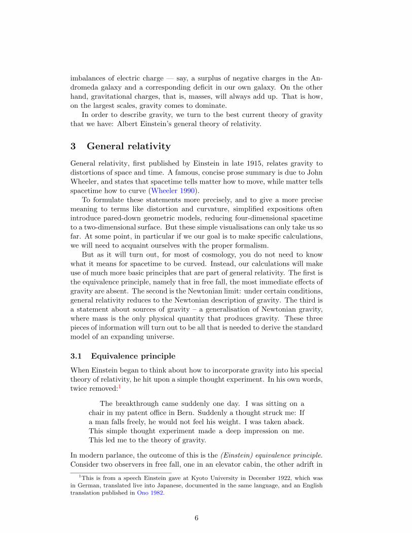
In the case of cosmology, the defining feature is scale. Figure 3 shows thevarious length scales, from the smallest objects we can still see with the naked

4

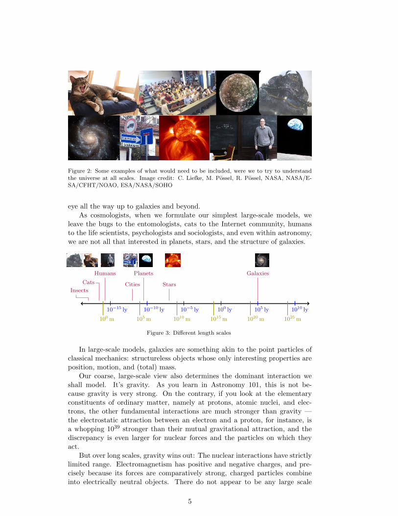
Figure 2: Some examples of what would need to be included, were we to try to understandthe universe at all scales. Image credit: C. Liefke, M. Possel, R. Possel, NASA, NASA/E-SA/CFHT/NOAO, ESA/NASA/SOHO

eye all the way up to galaxies and beyond.As cosmologists, when we formulate our simplest large-scale models, we

leave the bugs to the entomologists, cats to the Internet community, humansto the life scientists, psychologists and sociologists, and even within astronomy,we are not all that interested in planets, stars, and the structure of galaxies.

100 m 105 m 1010 m 1015 m 1020 m 1025 m

10−15 ly 10−10 ly 10−5 ly 100 ly 105 ly 1010 ly

Insects

Cats

Humans

Cities

Planets

Stars

Galaxies

Figure 3: Different length scales

In large-scale models, galaxies are something akin to the point particles ofclassical mechanics: structureless objects whose only interesting properties areposition, motion, and (total) mass.

Our coarse, large-scale view also determines the dominant interaction weshall model. It’s gravity. As you learn in Astronomy 101, this is not be-cause gravity is very strong. On the contrary, if you look at the elementaryconstituents of ordinary matter, namely at protons, atomic nuclei, and elec-trons, the other fundamental interactions are much stronger than gravity —the electrostatic attraction between an electron and a proton, for instance, isa whopping 1039 stronger than their mutual gravitational attraction, and thediscrepancy is even larger for nuclear forces and the particles on which theyact.

But over long scales, gravity wins out: The nuclear interactions have strictlylimited range. Electromagnetism has positive and negative charges, and pre-cisely because its forces are comparatively strong, charged particles combineinto electrically neutral objects. There do not appear to be any large scale

5

imbalances of electric charge — say, a surplus of negative charges in the An-dromeda galaxy and a corresponding deficit in our own galaxy. On the otherhand, gravitational charges, that is, masses, will always add up. That is how,on the largest scales, gravity comes to dominate.

In order to describe gravity, we turn to the best current theory of gravitythat we have: Albert Einstein’s general theory of relativity.

3 General relativity

General relativity, first published by Einstein in late 1915, relates gravity todistortions of space and time. A famous, concise prose summary is due to JohnWheeler, and states that spacetime tells matter how to move, while matter tellsspacetime how to curve (Wheeler 1990).

To formulate these statements more precisely, and to give a more precisemeaning to terms like distortion and curvature, simplified expositions oftenintroduce pared-down geometric models, reducing four-dimensional spacetimeto a two-dimensional surface. But these simple visualisations can only take us sofar. At some point, in particular if we our goal is to make specific calculations,we will need to acquaint ourselves with the proper formalism.

But as it will turn out, for most of cosmology, you do not need to knowwhat it means for spacetime to be curved. Instead, our calculations will makeuse of much more basic principles that are part of general relativity. The first isthe equivalence principle, namely that in free fall, the most immediate effects ofgravity are absent. The second is the Newtonian limit: under certain conditions,general relativity reduces to the Newtonian description of gravity. The third isa statement about sources of gravity – a generalisation of Newtonian gravity,where mass is the only physical quantity that produces gravity. These threepieces of information will turn out to be all that is needed to derive the standardmodel of an expanding universe.

3.1 Equivalence principle

When Einstein began to think about how to incorporate gravity into his specialtheory of relativity, he hit upon a simple thought experiment. In his own words,twice removed:1

The breakthrough came suddenly one day. I was sitting on achair in my patent office in Bern. Suddenly a thought struck me: Ifa man falls freely, he would not feel his weight. I was taken aback.This simple thought experiment made a deep impression on me.This led me to the theory of gravity.

In modern parlance, the outcome of this is the (Einstein) equivalence principle.Consider two observers in free fall, one in an elevator cabin, the other adrift in

1This is from a speech Einstein gave at Kyoto University in December 1922, which wasin German, translated live into Japanese, documented in the same language, and an Englishtranslation published in Ono 1982.

6

the cabin of a space-ship, far from any sources of gravity; these two cases areshown in figure 4.

Figure 4: Different observers in free fall: An observer in free fall in a gravitational field (left),and one who is far from any sources of gravity

A key question is: Can these two observers tell the difference? When theyperform physics experiments in their little cabins, can they tell whether or notthere are sources of gravity nearby?

To a large extent, the answer is no. After all, in free fall, the most commonindicators of a gravitational field are absent.

In everyday life, if I release a ball, it will fall to the ground. If I am in anelevator cabin in free fall, and gently release a ball, it will continue to float infront of me. Water will float, forming a wobbling giant droplet. If I positionmyself on a balance, that balance will show my weight to be zero. Behind allthis is the fact that, in a Newtonian gravitational field, objects that are in thesame place accelerate at the same rate.2

In fact, this rather good correspondence between a gravity-free situationand a free-fall situation is routinely used in physics. A widely known exampleis the International Space Station (ISS). At the cruising height of the ISS, at analtitude of about 400 km above sea level, the gravitational acceleration causedby the Earth is about 89% as strong as on Earth’s surface. The reason theastronauts, and all unattached objects around them, are floating is not becausegravity is weak, but because the ISS is in a free-fall orbit around Earth. Droptowers, where experiments are dropped inside a vacuum tube, can create similarmicrogravity conditions, albeit for a much shorter time of a few seconds, andin a much smaller volume.

2In the Newtonian picture, this is because the same object mass occurs both in the formulalinking force and acceleration, and in the formula specifying the gravitational force between apoint mass m and a much larger mass M . In the field of M , the point mass will be acceleratedin the radial direction as

a =1

mF = − 1

m

GMm

r2= −GM

r2,

which is independent of the object mass m.

7

Our first rough version of the principle tries to summarize these observationsas follows:

Einstein equivalence principle, draft version: Physics experimentsperformed by an observer in free fall will have the same outcome asexperiments performed by an observer who is infinitely far from allsources of gravity. In particular, the rules governing space and timeare those of special relativity.

3.2 Tidal forces and the limits of the equivalence principle

If we look more closely, we will soon realise that there are fundamental problemswith this version. Consider a truly gigantic elevator cabin falling towards Earth,with two giant spheres inside.3 What happens next is shown in figure 5. Clearly,

Figure 5: A giant cabin containing two spheres, falling towards Earth, shown here at sometime t1 (left) and at a later time t2 (right)

it’s becoming important that the two spheres are not both falling downwardson parallel trajectories. Instead, they both fall towards the center of the Earth.This falling motion brings them closer together over time, as the figure shows.This is an effect an observer inside the cabin can detect. He or she need onlylet these two spheres float, making sure that, initially, they are at rest relativeto each other, and wait until the two spheres have started to accelerate towardseach other. An observer drifting along in a space-ship, far removed from allsources of gravity, will not see this effect.

What the observer in free fall in a gravitational field sees, and the gravity-free observer doesn’t, are effects known as tidal effects, which are due to thefact that gravitational fields typically vary from location to location and/or over

3Worrying about the gigantic mass of such a cabin? That aspect of our thought experimentis admittedly inconsistent; so far, we have treated all falling particles as test particles, whoseown gravitational influence has no significant consequences. We will continue to do so. Justimagine that our giant cabin and giant spheres are made of truly fluffy, low-mass material.

8

time. As the term indicates, these varying gravitational fields are responsible forEarth’s tides. The main reason our home planet’s oceans have tides is becausethe Moon’s gravity acting on the water directly below is slightly stronger thanthe Moon’s gravity at the Earth’s center-of-mass, which in turn is stronger thanthe Moon’s gravity acting on water on the opposite side of the Earth.

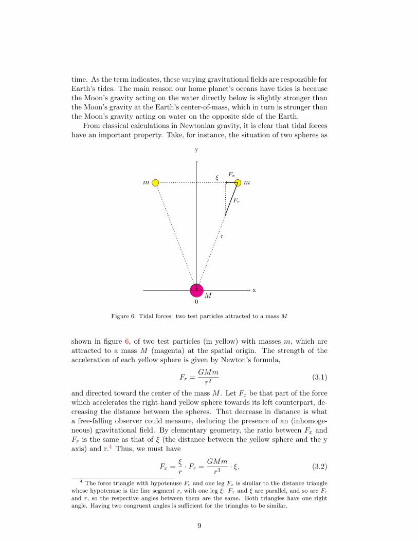
From classical calculations in Newtonian gravity, it is clear that tidal forceshave an important property. Take, for instance, the situation of two spheres as

mm

M0

x

y

r

ξ

Fr

Fx

Figure 6: Tidal forces: two test particles attracted to a mass M

shown in figure 6, of two test particles (in yellow) with masses m, which areattracted to a mass M (magenta) at the spatial origin. The strength of theacceleration of each yellow sphere is given by Newton’s formula,

Fr =GMm

r2(3.1)

and directed toward the center of the mass M . Let Fx be that part of the forcewhich accelerates the right-hand yellow sphere towards its left counterpart, de-creasing the distance between the spheres. That decrease in distance is whata free-falling observer could measure, deducing the presence of an (inhomoge-neous) gravitational field. By elementary geometry, the ratio between Fx andFr is the same as that of ξ (the distance between the yellow sphere and the yaxis) and r.4 Thus, we must have

Fx =ξ

r· Fr =

GMm

r3· ξ. (3.2)

4 The force triangle with hypotenuse Fr and one leg Fx is similar to the distance trianglewhose hypotenuse is the line segment r, with one leg ξ: Fx and ξ are parallel, and so are Fr

and r, so the respective angles between them are the same. Both triangles have one rightangle. Having two congruent angles is sufficient for the triangles to be similar.

9

Two properties of this result are typical for tidal forces: they fall of fasterthan the ordinary gravitational force when it comes to the distance r from thegravitational source, namely 1/r3 instead of 1/r2. And they are proportionalto the separation 2ξ of the two test masses whose relative distance they change.

Conversely, this means that tidal effects get smaller if we restrict our atten-tion to smaller regions of space. In a small region, only small separations 2ξare possible. Still, even a small acceleration will lead to considerable speeds,and observable effects, if we allow too much time to pass. We need to restrictobservation time, as well. All in all, we need to restrict our attention to a smallspacetime region.

3.3 The equivalence principle, reformulated

Even in a small, but finite spacetime region, there will in general be non-zerotidal effects. But in practice, our ability to detect small effects will be limited.All in all, here is a new version of the equivalence principle, which takes intoaccount the limitations imposed by tidal forces:

Einstein equivalence principle: Consider two observers whose mea-suring devices and instruments have a given limit of sensitivity.Then we can always find a maximum size S (defining spatial ex-tent as well as a maximum observation time), so that the followingholds: Physics experiments performed by the first observer in freefall in a restricted spacetime region of size S will have the sameoutcome as experiments performed by an observer in a restrictedspacetime region of size S who is infinitely far from all sources ofgravity. In particular, the rules governing space and time are thoseof special relativity.

In the infinitesimal limit, where we make the experimental region infinitelysmall, tidal forces vanish altogether. In this limit, the effects of tidal forcesare not even detectable with ideal measuring devices and instruments. This isless unrealistic than it sounds: Differential calculus teaches us about systematicways of describing the infinitesimally small.

In this modified version, the equivalence principle is quite useful. It providesguidance when it comes to finding general-relativistic versions of existing lawsof physics: If you know how these laws are defined in the context of specialrelativity, you know how these laws will be for a free-falling observer – at leastin an infinitesimal region.

This provides us with a powerful tool for deriving predictions of generalrelativity (or, for that matter, other theories as long as they incorporate theequivalence principle. In particular, the gravitational redshift of light in agravitational field can be derived directly from the equivalence principle (Schild1960, Schutz 1985, Schroter 2002).

3.4 Tidal deformations and attraction

So far, tidal forces have only been considered in their role as a limiting influence.Now, let us turn to what these forces actually do. Also, to be more precise,

10

we should talk about tidal accelerations – after all, in a gravitational field, theacceleration is independent of an object’s mass, and it makes sense to talk aboutgravitational acceleration, and the way it changes from location to location.

One effect, we have already seen: Two test masses, transversally separatedas they fall towards a point mass, will approach each other. There is anothereffect: the acceleration caused by the gravitational attraction of a point massdecreases with distance as 1/r2. Thus, the distance between two test massesthat are separated in the direction of their fall will increase, since the lower testmass feels a greater acceleration than the upper mass.

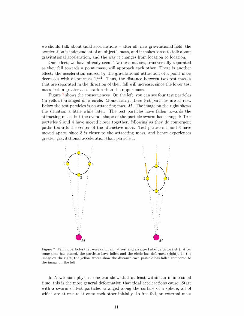
Figure 7 shows the consequences. On the left, you can see four test particles(in yellow) arranged on a circle. Momentarily, these test particles are at rest.Below the test particles is an attracting mass M . The image on the right showsthe situation a little while later. The test particles have fallen towards theattracting mass, but the overall shape of the particle swarm has changed: Testparticles 2 and 4 have moved closer together, following as they do convergentpaths towards the center of the attractive mass. Test particles 1 and 3 havemoved apart, since 3 is closer to the attracting mass, and hence experiencesgreater gravitational acceleration than particle 1.

M

1

3

42

M

1

3

42

Figure 7: Falling particles that were originally at rest and arranged along a circle (left). Aftersome time has passed, the particles have fallen and the circle has deformed (right). In theimage on the right, the yellow traces show the distance each particle has fallen compared tothe image on the left

In Newtonian physics, one can show that at least within an infinitesimaltime, this is the most general deformation that tidal accelerations cause: Startwith a swarm of test particles arranged along the surface of a sphere, all ofwhich are at rest relative to each other initially. In free fall, an external mass

11

configuration that is outside the particle sphere will deform the sphere into anellipsoid of the same volume. More concretely, the acceleration of the changein volume will initially be zero,5

V |t=0 = 0, (3.3)

where t = 0 is the time at which our particles were at rest relative to each other.The only time when tidal forces will change the volume of a sphere of

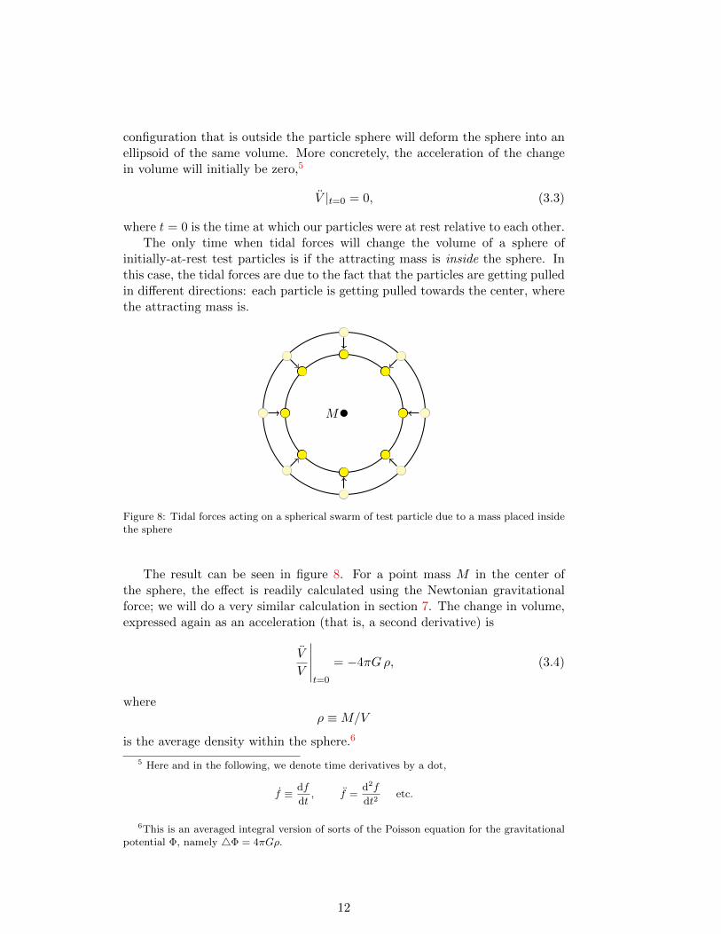
initially-at-rest test particles is if the attracting mass is inside the sphere. Inthis case, the tidal forces are due to the fact that the particles are getting pulledin different directions: each particle is getting pulled towards the center, wherethe attracting mass is.

M

Figure 8: Tidal forces acting on a spherical swarm of test particle due to a mass placed insidethe sphere

The result can be seen in figure 8. For a point mass M in the center ofthe sphere, the effect is readily calculated using the Newtonian gravitationalforce; we will do a very similar calculation in section 7. The change in volume,expressed again as an acceleration (that is, a second derivative) is

V

V

∣∣∣∣∣t=0

= −4πGρ, (3.4)

whereρ ≡M/V

is the average density within the sphere.6

5 Here and in the following, we denote time derivatives by a dot,

f ≡ df

dt, f =

d2f

dt2etc.

6This is an averaged integral version of sorts of the Poisson equation for the gravitationalpotential Φ, namely 4Φ = 4πGρ.

12

3.5 Newtonian limit and Einstein’s equation(s)

In the preceding sections, we have performed a number of calculations usingNewtonian gravity, and the concepts of motion and dynamics taken from clas-sical mechanics. How much of this carries over to general relativity?

Quite a lot, as it turns out. Historically, when Einstein developed generalrelativity, all but one of the many astronomical and terrestrial observations in-volving gravity were explained very accurately using Newtonian mechanics andthe Newtonian gravitational force. The one exception was the anomalous peri-helion advance of the planet Mercury, which Einstein took to be a fundamentaleffect, and used to shape his evolving theory of gravity.

But nonetheless, Newtonian gravity was highly successful. Any theory aim-ing to replace it had to be able to explain the successful predictions of Newtoniangravity. Under those conditions where the Newtonian predictions held — allof which involved comparatively weak gravitational fields, and objects movingmuch more slowly than c, the speed of light in vacuum — Einstein’s theoryneeded to include Newtonian gravity as a limiting case.

Elementary derivations of this Newtonian limit are a standard topic in text-books on general relativity. (“Post-Newtonian” derivations that not only showthe Newtonian limit, but add the various relativistic effects as a series develop-ment in 1/c2, are considerably more complicated; see e.g. Poisson 2014.)

Concerning the Einstein equivalence principle, we have seen that in a lo-cal, free-falling reference frame, physics is special-relativistic — at least up totidal forces, which can be kept arbitrarily small by restricting the spacetimeregion under consideration, but are always present to some degree. But clas-sical mechanics is itself a limit of special relativity, namely the limit where allparticle motion is slow compared with the vacuum speed of light. This suggeststhat free-falling systems are likely to have another interesting limit, at least aslong as this slow-motion condition is met: Whatever tidal forces remain can bedescribed using Newtonian gravity.

This is indeed the case, and even better: even allowing for fast-moving par-ticles, the full predictions of general relativity can be recovered with no morethan a simple change in the source term for gravitational attraction! Before wetalk about that simple change, for the record: The general description for howmatter and gravity are linked are Einstein’s equations, also called Einstein fieldequations (EFE), the centerpiece of his general theory of relativity; togetherwith the definition of the terms involved (including their physical interpreta-tion), they are general relativity. In their most general form, these equationscan be written as

Rµν −1

2Rgµν =

8πG

c4Tµν , (3.5)

where the Ricci tensor Rµν , Ricci scalar R and metric tensor gµν representspacetime geometry, while on the right-hand side, the energy-momentum tensorTµν describes mass, energy, momentum and pressure of the matter containedwithin spacetime. Each of the indices µ and ν can take on values between 0and 3, so equation (3.5) is really a concise way of writing 16 equations at once— or, in this case, 10 independent equations, since all terms involved remain

13

the same if we switch µ and ν. Together, these equations are the mathematicalembodiment of Wheeler’s summary of spacetime telling matter how to move,and matter telling spacetime how to curve.

As shown in a highly recommended article by Baez and Bunn 2005, fromthe full Einstein field equations linking spacetime curvature and the energy-momentum content of the spacetime, one can derive a much simpler form. Inorder to do so, one needs to go into free-fall and consider test particles arrangedinto a sphere. If these test particles are initially at rest relative to each other,one can show that the volume of the test particle sphere will change as

V

V

∣∣∣∣∣t=0

= −4πG (ρ+ [px + py + pz]/c2), (3.6)

where the average density ρ inside the test particle sphere includes contri-butions from all applicable kinds of energy (as per E = mc2), and where wehave added pressure terms px, py, pz for pressure into the x-, y-, and z-direction.Some additional information on the motivation of this in the context of specialrelativity is given in sections B.10 and B.7.

In the isotropic case, no direction is special, and we have px = py = pz = p,leading to the equation

V

V

∣∣∣∣∣t=0

= −4πG (ρ+ 3p/c2). (3.7)

As Bunn and Baez show, this form of Einstein’s equation can be used to re-derive Newton’s law of gravity for test particles surrounding a spherical mass.

If there is no mass, energy, pressure inside the test sphere, all that externalgravitational sources can do is deform the sphere, keeping its volume unchangedas per

V∣∣∣t=0

= 0. (3.8)

That is the simplest form of the vacuum Einstein’s equations.What should we make of the modified source terms in equations (3.6) and

(3.7)? Including energy as a source of gravity should come as no surprise, givenE = mc2. But energy, even in special relativity, is not a scalar quantity. Instead,it is one aspect of relativistic four-momentum, which includes both energy andmomentum. When we are looking at a gas, for instance, the particles involvedwill have energy as well as momentum. The latter becomes important wheneverthe particles bounce off the confining walls of a cylinder, creating pressure, or, inthe absence of a confining wall, for keeping track of what part of the momentumis flowing out of a particular region, or into it.

Given that energy and momentum are part of the same relativistic quantity,and pressure directly related to momentum, we should not be too surprisedthat, in a relativistic description, all these quantities occur together as sourcesof gravity.

14

3.6 What we need from general relativity

Now we have all that we will need from general relativity! We know that:

• in a reference frame in free fall, the laws of physics are almost the same asin special relativity; the deviations from special relativity are due to tidalforces, grow smaller as we look at smaller and smaller spacetime regions,and vanish as such a region becomes infinitesimally small.

• in such a reference frame in free fall, as long as all motions are muchslower than the vacuum speed of light c, what happens is described bythe Newtonian limit of general relativity, and can make use of Newtoniancalculations. Having all motions much slower than c also includes thecondition ρ p/c2 for pressure terms, since pressure is the result ofrandom particle motion.

• even if we have fast-moving matter (notably matter with a large pressurecomponent), the only correction to the usual Newtonian formula is thatthe source of gravity is not the mass density %M alone. It’s the massdensity %M+E including energy terms, and there is an extra pressure term,

%M → %M+E + 3p/c2, (3.9)

or the corresponding, slightly more complicated right-hand side of (3.6)for the non-isotropic case.

With this knowledge, let us consider cosmology.

4 A homogeneous, isotropic, expanding universe

What is the simplest realistic large-scale model of the universe as a whole? Asper our earlier considerations, we will be satisfied with our model representingonly the very largest scales, treating galaxies as point particles with no relevantinner structure. So how are galaxies distributed, at large scales? Figure 9shows two views of a wedge-like subregion of the universe, out to a distanceof 1.4 billion light-years, giving a good overview of the large-scale structure.7

Every blue dot is a galaxy; we as the observers are at the apex of the wedge.This is not perfectly, but fairly homogeneous, at least on average. On av-

erage, the properties of this universe are the same, regardless of an observer’slocation — or are they? At least from this wedge diagram, it’s not so easyto be sure one way or the other. For instance, the somewhat emptier regionnear the apex is due to the fact that the wedge is particularly slim near itsapex, thus contains fewer galaxies. The emptier regions at great distances, onthe other hand, are a typical selection effect. At greater distances, it is more

7 The diagram shows galaxies in the 2MASX catalogue (“2Micron All-Sky Survey, Extendedsource catalogue,” Jarrett et al. 2000) (catalog VII/233 on Vizier) that have an entry in theNED-D tabulation of extragalactic, redshift-independent distances, Version 14.1.0 February2017, http://ned.ipac.caltech.edu/Library/Distances/, as compiled by Ian Steer, Barry F.Madore, and the NED Team.

15

200400

600800

10001200

1400

0millio

n light-years

200 600 1000 14000

million light-years

Figure 9: Galaxy distribution in a wedge-like subregion of the universe: top view (top) andview from the side (bottom). Data from combining the NED distance catalogue and the2MASX catalogue, 25231 data points in total. We as the observers are at the point 0 at theapex of the wedge

difficult to detect, and measure the distances to, less luminous galaxies; thus,only the brighter very distant galaxies will be included in our catalogue. Inastronomy, this kind of selection effect due to brightness limitations is knownas Malmquist bias. Also, there are some radial strips where there are somewhatfewer galaxies, probably due to the fact that, in that particular direction, ourview into the distance is obscured by dust in our own galaxy.

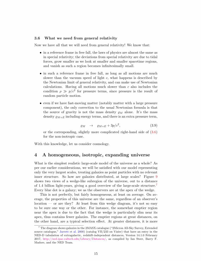
Figure 10 shows galaxies from the same data set in a rectangular box ofspace, viewed from the top. There are some hints of structure, some slightly-denser-than-average areas, but overall, the galaxy distribution looks fairly ho-mogeneous. There is no drastic clumping, say, with parts of the diagram devoidof galaxies altogether. Additional observations bear this out: Matter in our uni-verse is distributed fairly uniformly – at least on average, on sufficiently largescales.

Truly three-dimensional statements in astronomy are always difficult, sincedistance measurements are anything but easy. But there is one direct conse-quence of a homogeneous universe that is more straightforward to test. If theuniverse is basically the same everywhere, then the universe should look thesame, regardless where in the sky we point our telescopes. That is indeed thecase: In whatever direction we look, we will, on average, see the same numberof distant objects, with similar average properties. From our point of view,the universe is, on average, isotropic. (As an exercise, how are isotropy andhomogeneity related? Convince yourself that a universe that is isotropic for atleast two observers at different locations is necessarily isotropic, as well.)

16

-600 -500 -400 -300 -200 -100 0 100 200million light-years

400

500

600

700

800

900

mill

ion lig

ht-

years

Figure 10: Galaxy distribution in a box 800 times 500 times 30 million light-years in size;data and x-y coordinates are the same as in figure 9

Taking all these observations into account, we arrive at what HermannBondi, , in or before 1952, called the cosmological principle. In his own summary(“broadly speaking”; Bondi 1960), “[T]he universe presents the same aspectfrom every point except for local irregularities.” This extends the Copernicanprinciple, in that the Earth is nothing special — not when it comes to our homeplanet’s role in the solar system, nor when it comes to our position in the largeruniverse.

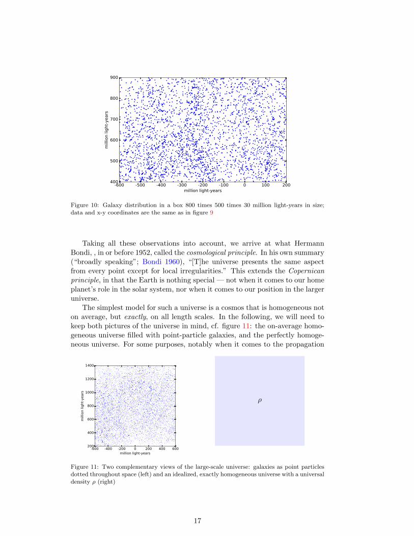
The simplest model for such a universe is a cosmos that is homogeneous noton average, but exactly, on all length scales. In the following, we will need tokeep both pictures of the universe in mind, cf. figure 11: the on-average homo-geneous universe filled with point-particle galaxies, and the perfectly homoge-neous universe. For some purposes, notably when it comes to the propagation

-600 -400 -200 0 200 400 600million light-years

200

400

600

800

1000

1200

1400

mill

ion lig

ht-

years

ρ

Figure 11: Two complementary views of the large-scale universe: galaxies as point particlesdotted throughout space (left) and an idealized, exactly homogeneous universe with a universaldensity ρ (right)

17

of light, we will keep talking about separate galaxies. We will be asking, forinstance, how long it takes light to travel from one galaxy to another, and howthat light is redshifted. Let us call this the galaxy dust picture of the universe.But when we talk about overall properties of the universe, such as the densityvalues for matter or radiation, we will switch to the continuum picture. We willassume that the density is constant throughout the universe; after all, that iswhat (idealized) homogeneity means.

If you take these pictures too literally, they contradict each other. But youshouldn’t, really. Both are models, which are meant to map certain aspectsof the large-scale universe. Physicists are allowed to use models — simple, yetsuitable models are what allows us to make powerful and predictive calculationsin the first place!

4.1 What can change in a homogeneous universe?

The homogeneity condition is a powerful constraint on how the universe canchange over time. If we demand continued homogeneity, certain types of changeare ruled out. After all, in that case, matter cannot move in any way that resultsin large-scale inhomogeneities.

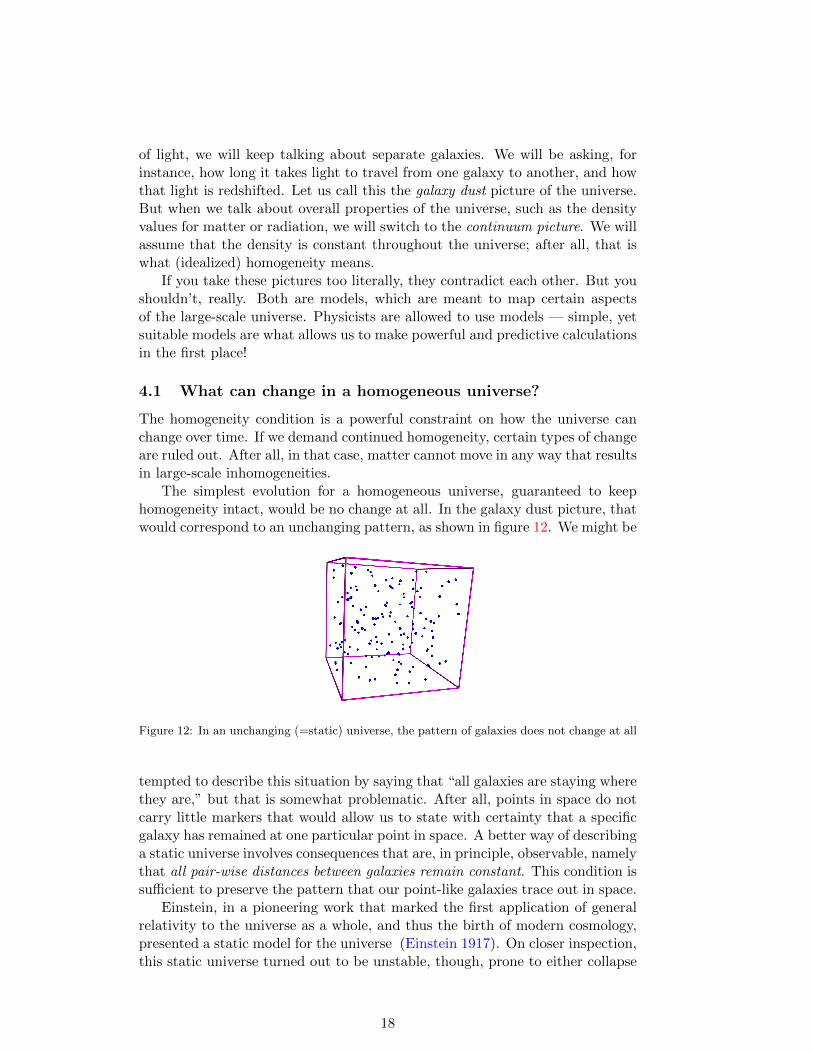
The simplest evolution for a homogeneous universe, guaranteed to keephomogeneity intact, would be no change at all. In the galaxy dust picture, thatwould correspond to an unchanging pattern, as shown in figure 12. We might be

Figure 12: In an unchanging (=static) universe, the pattern of galaxies does not change at all

tempted to describe this situation by saying that “all galaxies are staying wherethey are,” but that is somewhat problematic. After all, points in space do notcarry little markers that would allow us to state with certainty that a specificgalaxy has remained at one particular point in space. A better way of describinga static universe involves consequences that are, in principle, observable, namelythat all pair-wise distances between galaxies remain constant. This condition issufficient to preserve the pattern that our point-like galaxies trace out in space.

Einstein, in a pioneering work that marked the first application of generalrelativity to the universe as a whole, and thus the birth of modern cosmology,presented a static model for the universe (Einstein 1917). On closer inspection,this static universe turned out to be unstable, though, prone to either collapse

18

or expand, at any rate: it would depart from its static state in response to thesmallest perturbations (Eddington 1930).

What, then, is the next simplest kind of change that preserves homogeneity?It is when all pairwise distances between galaxies change in the same way, inproportion to one and the same time-dependent factor a(t), commonly calledthe (universal) cosmic scale factor, which depends on a suitably defined time

Figure 13: Expansion with a universal scale factor: a portion of the universe, pictured at anearlier (left) and a later time (right)

parameter t that is commonly called cosmic time (about which more below).That way, ratios between pair-wise galaxy distances do not change over time.The pattern of all these galaxies’ locations in space does not change except forits overall scale. In an expanding universe as in figure 13, all distances becomelarger over time. But in terms of preserving homogeneity, a contracting universewhere all distances shrink in proportion to the same scale factor works just aswell.

The systematic motions associated with scale-factor expansion, and its char-acteristic change of pair-wise distances, is called the Hubble flow. Galaxieswhose pair-wise distances change in exactly the way described by a changingoverall scale factor are said to be “in the Hubble flow” or “part of the Hubbleflow.” These systematic pair-wise distance changes are what is meant whencosmologists talk about cosmic expansion.

The motions of real galaxies can deviate from the Hubble flow for differentreasons. Many are part of galaxy clusters, orbiting each other; in this case,while the cluster’s center of mass is in the Hubble flow, individual galaxies’motions will be slightly different. And even galaxies that are not in a cluster(so-called “field galaxies”) will typically deviate from the Hubble flow at leasta little bit. Collectively, these deviations from the Hubble flow are known aspeculiar motion. In the following sections, we will disregard peculiar motion,and assume that all galaxies are faithfully following the Hubble flow.

A natural follow-up question is the following: In an expanding cosmos, whatabout bound systems? Do galaxies themselves grow larger, too? How abouthumans? Or atoms? This question is particularly natural whenever cosmicexpansion is explained in terms like “space itself is expanding” — languagewhich I have avoided, precisely because I think that it leads to misconceptions,and does not evoke a faithful image of what is happening. I will address the

19

question of bound systems, and what happens to them during cosmic expansion,later on in section 8.2.

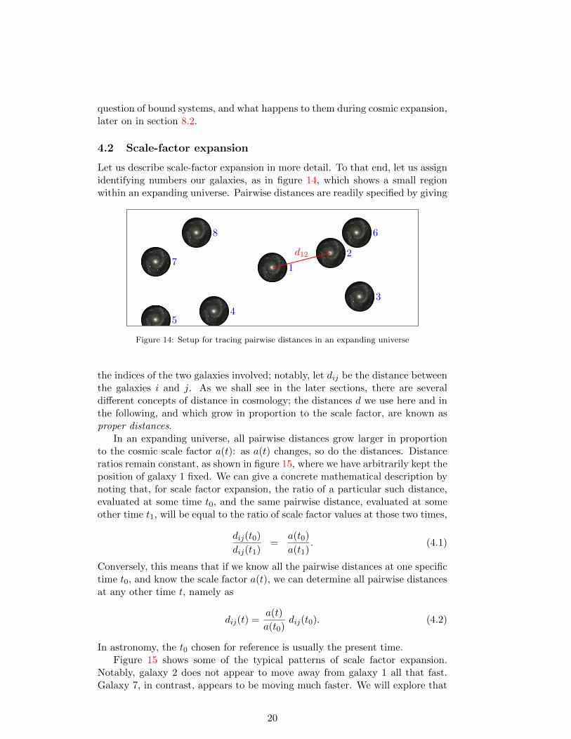
4.2 Scale-factor expansion

Let us describe scale-factor expansion in more detail. To that end, let us assignidentifying numbers our galaxies, as in figure 14, which shows a small regionwithin an expanding universe. Pairwise distances are readily specified by giving

1

2

3

45

6

7

8

d12

Figure 14: Setup for tracing pairwise distances in an expanding universe

the indices of the two galaxies involved; notably, let dij be the distance betweenthe galaxies i and j. As we shall see in the later sections, there are severaldifferent concepts of distance in cosmology; the distances d we use here and inthe following, and which grow in proportion to the scale factor, are known asproper distances.

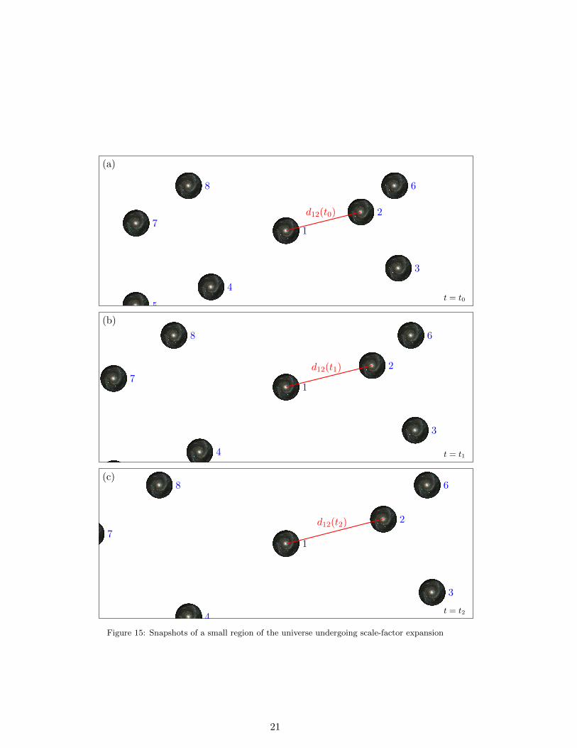
In an expanding universe, all pairwise distances grow larger in proportionto the cosmic scale factor a(t): as a(t) changes, so do the distances. Distanceratios remain constant, as shown in figure 15, where we have arbitrarily kept theposition of galaxy 1 fixed. We can give a concrete mathematical description bynoting that, for scale factor expansion, the ratio of a particular such distance,evaluated at some time t0, and the same pairwise distance, evaluated at someother time t1, will be equal to the ratio of scale factor values at those two times,

dij(t0)

dij(t1)=

a(t0)

a(t1). (4.1)

Conversely, this means that if we know all the pairwise distances at one specifictime t0, and know the scale factor a(t), we can determine all pairwise distancesat any other time t, namely as

dij(t) =a(t)

a(t0)dij(t0). (4.2)

In astronomy, the t0 chosen for reference is usually the present time.Figure 15 shows some of the typical patterns of scale factor expansion.

Notably, galaxy 2 does not appear to move away from galaxy 1 all that fast.Galaxy 7, in contrast, appears to be moving much faster. We will explore that

20

(a)

1

2

3

4

5

6

7

8

t = t0

d12(t0)

(b)

1

2

3

4

5

6

7

8

t = t1

d12(t1)

(c)

1

2

3

4

5

6

7

8

t = t2

d12(t2)

Figure 15: Snapshots of a small region of the universe undergoing scale-factor expansion

21

systematic correlation in section 5. But before we do, it’s time for a closer lookat the parameter t.

4.3 Cosmic time t and proper distance d

So far, we have introduced the cosmic time t only via the cosmic scale factora(t), and we have implicitly assumed that t is a useful time coordinate, to beused in statements like “the position of galaxy i at time t0” or about positionschanging with time. Likewise, we have blithely talked about (proper) distancesd as if that were a well-defined concept.

If the only purpose of t were to parametrize the universal scale factor a,then any other t′ = f(t), with f a monotonically increasing function (i.e. afunction with derivative df/dt > 0 everywhere) would serve as well. But t canbe defined to be much more than an arbitrary parameter.

In order to connect t to the physical concept of time, let us zoom in on oneof our galaxies. For each galaxy, we can define a notion of time by consideringclocks that are moving along with the galaxy in question — for each galaxy, weconsider a clock that is at rest relative to that galaxy. Time as measured by anobject’s co-moving clock is called that object’s proper time. In the vicinity ofone particular galaxy, we can see how a(t) changes, and we can determine howthe proper time clock ticks. So why not combine the two, and use that galaxy’sproper time to parametrize the scale factor a(t)?

If we do so for one galaxy, though, the same needs to hold for every othergalaxy in the Hubble flow, as well. After all, in our simplified model, theuniverse is homogeneous. No location, no galaxy is special. If the parameter t ina(t) corresponds to proper time for one particular galaxy, it must correspond toproper time for any other galaxy in the Hubble flow. Otherwise, we could devisean experiment, namely comparing the evolution of a(t) with the passage ofproper time, that would have different outcomes depending on where, in whichgalaxy, we perform the experiment. In other words, the physical propertiesof our cosmos would vary with location, which would make the universe inquestion inhomogeneous.

Note that, by defining cosmic time in this manner, we have also implicitlysupplied another necessary part of defining a global time coordinate: a definitionof simultaneity. Switching to the continuum picture, we can track how thedensity of the universe ρ(t) changes over time. In a homogeneous universe,by definition, ρ(t) at some constant time t will be the same at any location,wherever we measure the local density. You can turn this around, and use ρvalues to define which events in our universe are simultaneous.8

Note that, given our particular definition, the global time coordinate t willhave some unusual properties. Recall that in special relativity, we have the effectof time dilation: when inertial observers in relative motion use their reference

8In fact, the proper relativistic definition is that a homogeneous universe is a universe inwhich it is possible to define simultaneity in such a way that the local density ρ will havethe same value at all simultaneous events. Exercise: Convince yourself using reasoning fromspecial relativity that in a homogeneous universe, an observer moving relative to the mattercontent of the cosmos will detect local inhomogeneities on a large scale.

22

frames to describe each other’s (proper time) clocks, each will deduce thatthe other’s clocks are ticking more slowly than his own, giving rise to directlyobservable effects as in the case of the space-travelling twin (cf. section B.4 fora lightning review of the pertinent concepts of special relativity). If one were tocombine such clocks in relative motion, the result would be markedly differentfrom any of the usual time coordinates defined by inertial observers. Statementsthat are true using the usual inertial time coordinates, notably those about themotion of light or material objects, do not necessarily hold for such an unusualcombined time coordinate.9

Similarly, in defining cosmic time to correspond to proper time for all galax-ies in the Hubble flow, we have created such an unusual “compound time coor-dinate”. As long as we restrict our attention to a single galaxy and its directneighbourhood, we can invoke the equivalence principle. Our cosmic time coor-dinate, which in that neighbourhood corresponds to that galaxy’s proper time,can be used in calculations of speeds, accelerations and the like. But as soonas we zoom out and consider t as a global coordinate, we need to be careful.

Also, we should not forget that the choice of time coordinate affects thenotion of distance. Whenever we talk about the distance of two galaxies atcosmic time t, we are implicitly defining a three-dimensional space, namely thesubset of all points in spacetime that have this particular value of the cosmictime coordinate. Choose an unusual time coordinate, and that subset, in otherwords: space, will have unusual properties as well. At small scales, all should bewell, in line with the equivalence principle. But as one goes to larger distances,these distances need to be interpreted carefully. They will not, in general,correspond to ordinary physical distances, and their derivatives with respect tocosmic time will not, in general, correspond to physical speeds.

In conclusion, cosmic time t is an unusual coordinate, and we must be carefulnot make unwarranted assumptions about how physical systems behave whendescribed using a coordinate of this kind.

5 The Hubble relation

Back to galaxies in the expanding universe. Figure 15, with its snapshots ofa universe that is undergoing scale-factor expansion, illustrates a systematiccorrelation: Galaxies that are further away from our spatial origin (arbitrarilychosen to be at the location of galaxy 1) move faster than their less distant kin.

The reason behind this is, of course, the unusual pattern of motions wheredistances change in proportion to one and the same factor. If I multiply adistance of 100 million light-years by a factor of 1.3 (corresponding to thescale-factor change between panels a and c of figure 15), The 100 become 130million light-years, and absolute difference of 30 million light-years.

If I multiply 200 million light-years by the same factor, the absolute differ-

9In fact, if you combine inertial time coordinates of systems in relative motion in this way,you will end up with a toy model that mimics most of the defining properties of moderncosmological models — using mathematical tools no more complicated than the simplest formof the Lorentz transformations, and solving linear equations (Possel 2017).

23

ence is twice as large, namely 60 million light-years. The larger the originaldistance, the larger the absolute difference — and since these changes happenduring the same period of time, we also have: the larger the original distance,the larger the rate of change of the distance.

We can make this more precise as follows: Consider any pair-wise distancedij(t), which changes as specified in equation (4.2). Then we can calculate therate of change, namely the derivative with respect to the time coordinate, as

vij(t) ≡ dij(t) =d

dt

(a(t)

a(t0)dij(t0)

)=

a(t)

a(t0)dij(t0)

=a(t)

a(t)

a(t)

a(t0)dij(t0) =

a(t)

a(t)dij(t). (5.1)

The function

H(t) ≡ a(t)

a(t)(5.2)

is called the Hubble parameter, and its value at the present time t0,

H0 ≡ H(t0) =a(t)

a(t)

∣∣∣∣t=t0

(5.3)

is the Hubble constant. The relation

vij(t) = H(t) · dij(t) (5.4)

is called the Hubble relation. Sometimes, instead of the Hubble constant H0,astronomers will use the (dimensionless) reduced Hubble constant h defined by

H0 = h · 100km/s

Mpc, (5.5)

where 1 Mpc (“mega-parsec”), a distance measure commonly used in astron-omy, corresponds to 3.26 million light-years. Typical Hubble constant valuesare such that the reduced Hubble constant is around h ≈ 0.7.

Naively, the Hubble relation is a relation between pair-wise relative velocitiesand pair-wise distances, valid at any specific time t. Whenever we can determinethese distances and velocities, the expanding universe model predicts a clearrelationship between the two – a prediction to be tested against observationaldata. In particular, if we take one of the two galaxies to be our own, thenequation (5.4) is a relation between distant galaxies’ distances from us and thesegalaxies’ radial velocities; since, in an expanding universe, those velocities areaway from us, they are commonly called recession speeds.

But taking into account the unusual properties of the cosmic time t dis-cussed in section 4.3, we know to be be cautious. In particular, there is noreason to think that on large scales, the cosmic-time derivatives of the quan-tities dij correspond to a relativistic generalisation of the concept of relativespeed. Closer examination shows that they do not. There is, in fact, a sensiblerelativistic generalisation of the concept of relative speeds for the situation of

24

two galaxies exchanging light signals in an expanding universe, and it gives aresult that is very different from the cosmic-time derivative of the correspondingdij (Narlikar 1994, Bunn and Hogg 2009). In fact, the most obvious propertyunbecoming a relativistic relative speed, namely the fact that by the Hubblerelation is that we can have vij > c for sufficiently large distances dij , whichtaken at face value would mean superluminal motion. This is a direct indicationthat vij is no generalised relativistic relative speed.

In the direct cosmic neighbourhood of each free-falling galaxy in the Hubbleflow, on the other hand, cosmic time t is a good approximation for the usualtime coordinate of special relativity and classical mechanics. There, the inter-pretation of the Hubble relation as linking our usual notion of distances andrelative speeds is valid. This is true in the cosmic neighbourhood of our owngalaxy, and in this approximation, we can link the Hubble relation to an actualobservable: the redshift of light reaching us from another galaxy.

5.1 Free-falling galaxies and the Doppler effect

All the galaxies in our simplified model are in free fall, so the crucial conditionfor applying the equivalence principle is fulfilled: at least in the direct vicinityof each galaxy, the laws of special relativity should hold – limited by any tidalforces that might be present. We know from the Hubble relation (5.4) that inthe close vicinity of that galaxy, all distance changes happen rather slowly. Infact, by focusing on a sufficiently small region of space we can ensure that all thedij , and consequently all vij , are below some given limit. Given the observedvalue of the Hubble constant, of around 20 km/s per million light-years, evengalaxies as far away as 140 million light-years will not reach recession speedvalues of more than about 1 percent of the speed of light in vacuum.

In this limit we can talk about motion in the usual way of classical physics —we can talk about galaxies moving, and about light travelling from one galaxyto another along straight lines at the speed c, about dij being an ordinarydistance to be covered, and about t behaving like an ordinary time coordinate.In this limit, we will also find that the light from distant galaxies is subject tothe (classical) Doppler shift.

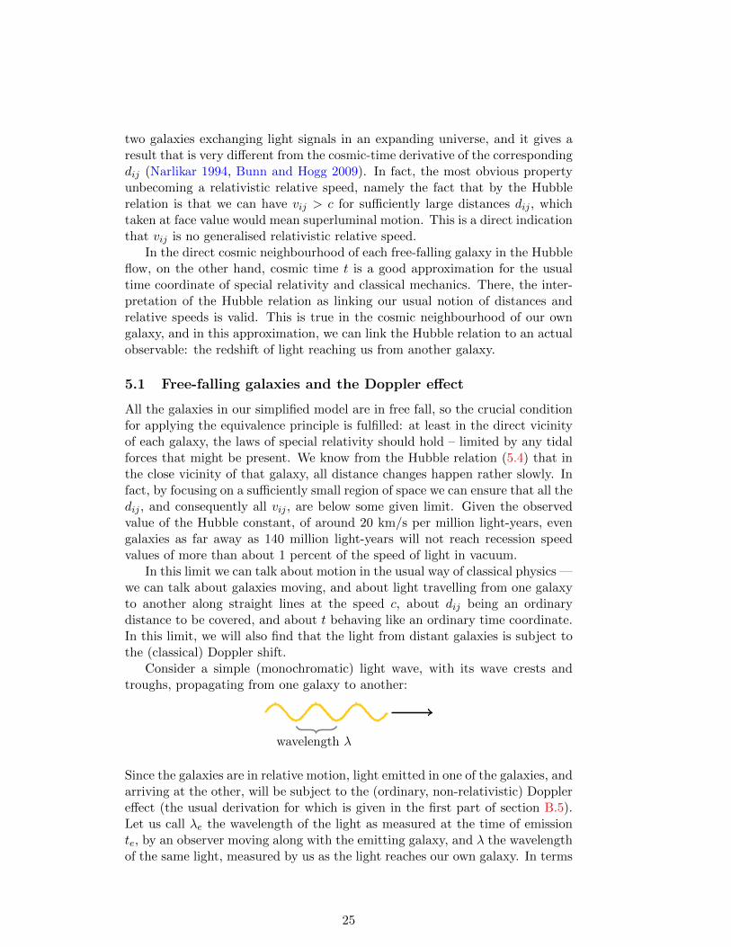
Consider a simple (monochromatic) light wave, with its wave crests andtroughs, propagating from one galaxy to another:

wavelength λ

Since the galaxies are in relative motion, light emitted in one of the galaxies, andarriving at the other, will be subject to the (ordinary, non-relativistic) Dopplereffect (the usual derivation for which is given in the first part of section B.5).Let us call λe the wavelength of the light as measured at the time of emissionte, by an observer moving along with the emitting galaxy, and λ the wavelengthof the same light, measured by us as the light reaches our own galaxy. In terms

25

of these quantities, the redshift z is defined as

z =λ− λeλe

. (5.6)

The classical Doppler effect links z with the emitting object’s radial speed v(that is, the component of its speed directly away from us or, for negativevalues, directly towards us) as

z =v

c. (5.7)

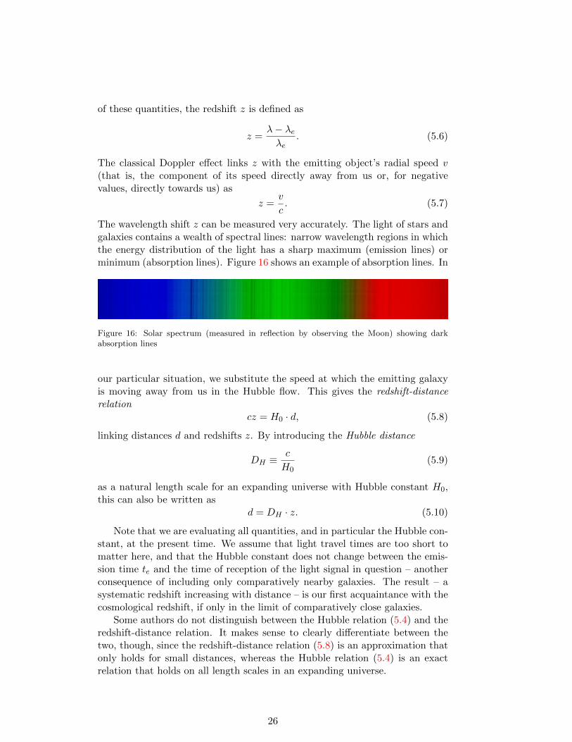
The wavelength shift z can be measured very accurately. The light of stars andgalaxies contains a wealth of spectral lines: narrow wavelength regions in whichthe energy distribution of the light has a sharp maximum (emission lines) orminimum (absorption lines). Figure 16 shows an example of absorption lines. In

Figure 16: Solar spectrum (measured in reflection by observing the Moon) showing darkabsorption lines

our particular situation, we substitute the speed at which the emitting galaxyis moving away from us in the Hubble flow. This gives the redshift-distancerelation

cz = H0 · d, (5.8)

linking distances d and redshifts z. By introducing the Hubble distance

DH ≡c

H0(5.9)

as a natural length scale for an expanding universe with Hubble constant H0,this can also be written as

d = DH · z. (5.10)

Note that we are evaluating all quantities, and in particular the Hubble con-stant, at the present time. We assume that light travel times are too short tomatter here, and that the Hubble constant does not change between the emis-sion time te and the time of reception of the light signal in question – anotherconsequence of including only comparatively nearby galaxies. The result – asystematic redshift increasing with distance – is our first acquaintance with thecosmological redshift, if only in the limit of comparatively close galaxies.

Some authors do not distinguish between the Hubble relation (5.4) and theredshift-distance relation. It makes sense to clearly differentiate between thetwo, though, since the redshift-distance relation (5.8) is an approximation thatonly holds for small distances, whereas the Hubble relation (5.4) is an exactrelation that holds on all length scales in an expanding universe.

26

5.2 Measuring astronomical distances

Determining distances is one of the more difficult problems in astronomy. Ourbest current solution is the cosmic distance ladder: a combination of variousmethods used by astronomers to successively determine distances within ourcosmic neighbourhood and beyond (de Grijs 2011). The term derives from thefact that the different methods for determining astronomical distances buildone upon the other, representing the consecutive “ladder steps”.

The first steps involve measurements to establish the distance scale withinthe solar system, notably the average Earth-Sun distance, which is known asthe astronomical unit. The traditional method for determining this basic scalemade use of parallax measurements (corresponding to the way astronomicalobservations change as the observer changes location), notably during Venustransits in front of the Sun. Modern measurements are based on the light-travel time of radar signals sent to the nearest planets. The next step involvesmeasurements of stellar parallax, that is, the change in the stars’ apparentpositions as the Earth orbits the Sun. At the time of this writing, ESA’s Gaiamission is measuring highly accurate distances to more than a billion stars inthis way.

With accurate parallax measurements, one can hope to eliminate what usedto be some extra steps of the ladder; in any case, extragalactic distances typ-ically involve what are known as standard candles: objects whose total lightoutput per unit time, that is, each object’s luminosity, is known, either becauseall objects of a certain type have the same luminosity, or because the luminositycan be derived from certain observable properties of the object.

Of great importance, both historically and for the modern distance scale,are Cepheid variables. The luminosity of these comparatively rare, massiveand bright stars changes periodically over time, with periods between days andmonths. The change is caused by an overall pulsation of the star: as the star getsbigger, it gets brighter. Size and time-scale are related, and so are the pulsationperiod and the star’s brightness (both average and maximal/minimal).

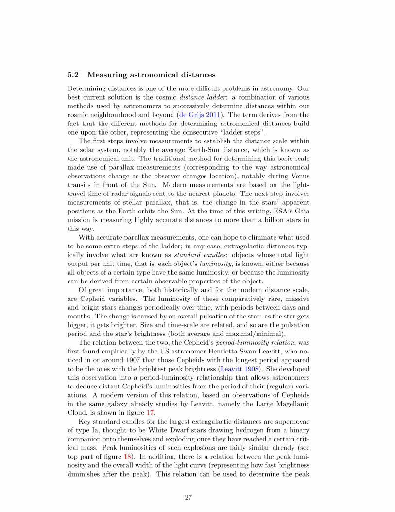
The relation between the two, the Cepheid’s period-luminosity relation, wasfirst found empirically by the US astronomer Henrietta Swan Leavitt, who no-ticed in or around 1907 that those Cepheids with the longest period appearedto be the ones with the brightest peak brightness (Leavitt 1908). She developedthis observation into a period-luminosity relationship that allows astronomersto deduce distant Cepheid’s luminosities from the period of their (regular) vari-ations. A modern version of this relation, based on observations of Cepheidsin the same galaxy already studies by Leavitt, namely the Large MagellanicCloud, is shown in figure 17.

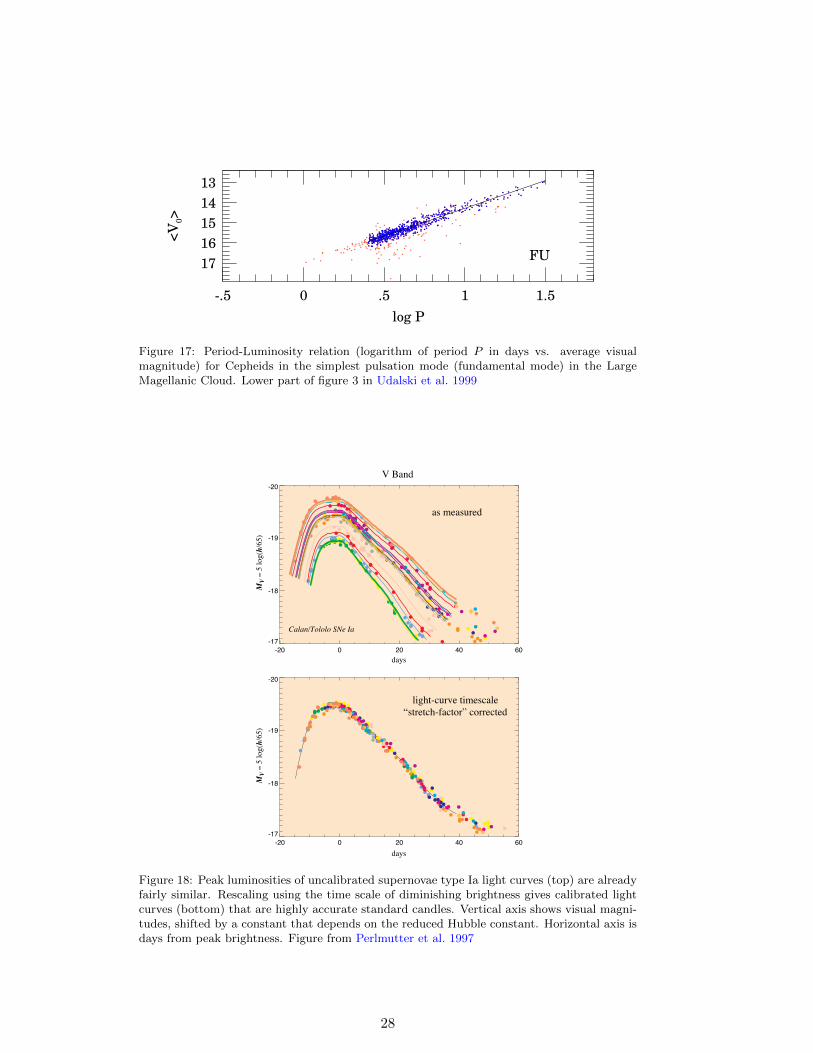
Key standard candles for the largest extragalactic distances are supernovaeof type Ia, thought to be White Dwarf stars drawing hydrogen from a binarycompanion onto themselves and exploding once they have reached a certain crit-ical mass. Peak luminosities of such explosions are fairly similar already (seetop part of figure 18). In addition, there is a relation between the peak lumi-nosity and the overall width of the light curve (representing how fast brightnessdiminishes after the peak). This relation can be used to determine the peak

27

Vol. 49 213

17

16

15

14

13

<V

0>

LMC Cepheids

-.5 0 .5 1 1.5

17

16

15

14

13<

V0>

FU

log P

Fig. 3. Upper panel: V-band P–L relation of the LMC Cepheids. Darker and lighter dots indicate FUand FO mode Cepheids, respectively. Lower panel: P–L relation for the FU Cepheids. Solid lineindicates adopted approximation (Table 2). Dark and light dots correspond to stars used and rejectedin the final fit, respectively.

16

14

12

<W

I>

LMC Cepheids

-.5 0 .5 1 1.5

16

14

12

<W

I>

FU

log P

Fig. 4. Upper panel: WI index P–L relation of the LMC Cepheids. Darker and lighter dots indicateFU and FO mode Cepheids, respectively. Lower panel: P–L relation for the FU Cepheids. Solid lineindicates adopted approximation (Table 2). Dark and light dots correspond to stars used and rejectedin the final fit, respectively.

Figure 17: Period-Luminosity relation (logarithm of period P in days vs. average visualmagnitude) for Cepheids in the simplest pulsation mode (fundamental mode) in the LargeMagellanic Cloud. Lower part of figure 3 in Udalski et al. 1999

0.6 0.70.5 0.8 0.90.40.30.20.10.0

2

1

3

5

7

9

10

11

12

13

14

8

6

4

0

Dec

. 1

99

5 S

Ne

Mar

. 1

99

6 S

Ne

Redshift

NSN

Redshifts

-20 0 20 40 60

-17

-18

-19

-20

-20 0 20 40 60

-17

-18

-19

-20

V Band

as measured

light-curve timescale

“stretch-factor” corrected

days

MV

– 5

lo

g(h

/65

)

days

MV

– 5

lo

g(h

/65

)

Calan/Tololo SNe Ia

Low Redshift Type Ia Template Lightcurves

http://www-supernova.lbl.gov/

C. Pennypacker M. DellaValle R. Ellis, R. McMahon Univ. of Padova IoA, Cambridge

B. Schaefer P. Ruiz-Lapuente H. Newberg Yale University Univ. of Barcelona Fermilab

We have discovered well over 50 high redshift Type Ia supernovae so

far. Of these, approximately 50 have been followed with spectroscopy

and photometry over two months of the light curve. The redshifts

shown in this histogram are color coded to show the increasing depth

of the search with each new “batch” of supernova discoveries. The

most recent supernovae, discovered the last week of 1997, are now

being followed over their lightcurves with ground-based and (for those

labeled “HST”) with the Hubble Space Telescope.

Type Ia supernovae observed “nearby” show a relationship between

their peak absolute luminosity and the timescale of their light curve: the

brighter supernovae are slower and the fainter supernovae are faster (see

Phillips, Ap.J.Lett., 1993 and Riess, Press, & Kirshner, Ap.J.Lett.,

1995). We have found that a simple linear relation between the absolute

magnitude and a “stretch factor” multiplying the lightcurve timescale

fits the data quite well until over 45 restframe days past peak. The lower

plot shows the “nearby” supernovae from the upper plot, after fitting

and removing the stretch factor, and “correcting” peak magnitude with

this simple calibration relation.

Mar

. 1

99

7 S

Ne

Dec. 1997 SNe

Jan

. 1

99

7 S

Ne

Fir

st 7

SN

e

HST

HST

HST

HST

HST

Figure 18: Peak luminosities of uncalibrated supernovae type Ia light curves (top) are alreadyfairly similar. Rescaling using the time scale of diminishing brightness gives calibrated lightcurves (bottom) that are highly accurate standard candles. Vertical axis shows visual magni-tudes, shifted by a constant that depends on the reduced Hubble constant. Horizontal axis isdays from peak brightness. Figure from Perlmutter et al. 1997

28

brightness more accurately, resulting in calibrated supernova Ia light curvesthat are fairly accurate standard candles (bottom part of figure 18), which playa key role for modern cosmological observations.

Standard candles are useful for determining distances since the apparentbrightness of an object of given luminosity is a direct measure of that object’sdistance from us. This is a matter of everyday experience – we perceive aflashlight that is directly in front of us as much brighter than the same flashlighta hundred meters away.

The relation between luminosity, distance, and flux density can be moreprecise in the following way. We had already defined the luminosity, the amountof energy emitted by an object per unit time, as a physical measure of anobject’s intrinsic brightness. For the apparent brightness, we need to measurethe amount of radiation we receive from a distant object.

But that amount will depend on our collecting area – within any givenperiod of time, larger telescopes collect more light than smaller telescopes. Thephysical measure of the apparent brightness of an observed object is thus whatis known in technical terms as the irradiance or (radiation) flux density: theamount of radiation energy received per unit time, per unit area.

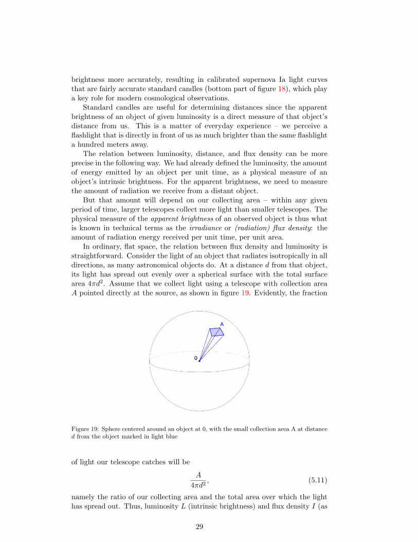
In ordinary, flat space, the relation between flux density and luminosity isstraightforward. Consider the light of an object that radiates isotropically in alldirections, as many astronomical objects do. At a distance d from that object,its light has spread out evenly over a spherical surface with the total surfacearea 4πd2. Assume that we collect light using a telescope with collection areaA pointed directly at the source, as shown in figure 19. Evidently, the fraction

Figure 19: Sphere centered around an object at 0, with the small collection area A at distanced from the object marked in light blue

of light our telescope catches will be

A

4πd2, (5.11)

namely the ratio of our collecting area and the total area over which the lighthas spread out. Thus, luminosity L (intrinsic brightness) and flux density I (as

29

a measure of apparent brightness) are related by the inverse square law

I =L

4πd2. (5.12)

This relation is the basis of standard candle distance measurements: Determinethe luminosity L from the properties of the standard candle, measure the fluxdensity I directly using a telescope, and you can solve equation (5.12) for thedistance.

At least, this is true for our cosmic neighbourhood, up to distances of afew hundred million light-years. For very distant objects, there is a modifiedinverse square law, which we will derive below, in section 6.7.

5.3 Measuring the Hubble constant

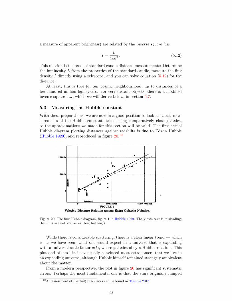
With these preparations, we are now in a good position to look at actual mea-surements of the Hubble constant, taken using comparatively close galaxies,so the approximations we made for this section will be valid. The first actualHubble diagram plotting distances against redshifts is due to Edwin Hubble(Hubble 1929), and reproduced in figure 20.10

ASTRONOMY: E. HUBBLE

corrected for solar motion. The result, 745 km./sec. for a distance of1.4 X 106 parsecs, falls between the two previous solutions and indicatesa value for K of 530 as against the proposed value, 500 km./sec.

Secondly, the scatter of the individual nebulae can be examined byassuming the relation between distances and velocities as previouslydetermined. Distances can then be calculated from the velocities cor-rected for solar motion, and absolute magnitudes can be derived from theapparent magnitudes. The results are given in table 2 and may becompared with the distribution of absolute magnitudes among the nebulaein table 1, whose distances are derived from other criteria. N. G. C. 404

o~~~~~~~~~~~~~~~~

0.

S0OKM

0

DISTANCE0 IDPARSEC S 2 ,10 PARSECS

FIGURE 1

Velocity-Distance Relation among Extra-Galactic Nebulae.Radial velocities, corrected for solar motion, are plotted against

distances estimated from involved stars and mean luminosities ofnebulae in a cluster. The black discs and full line represent thesolution for solar motion using the nebulae individually; the circlesand broken line represent the solution combining the nebulae intogroups; the cross represents the mean velocity corresponding tothe mean distance of 22 nebulae whose distances could not be esti-mated individually.

can be excluded, since the observed velocity is so small that the peculiarmotion must be large in comparison with the distance effect. The objectis not necessarily an exception, however, since a distance can be assignedfor which the peculiar motion and the absolute magnitude are both withinthe range previously determined. The two mean magnitudes, - 15.3and - 15.5, the ranges, 4.9 and 5.0 mag., and the frequency distributionsare closely similar for these two entirely independent sets of data; andeven the slight difference in mean magnitudes can be attributed to theselected, very bright, nebulae in the Virgo Cluster. This entirely unforcedagreement supports the validity of the velocity-distance relation in a very

PRoc. N. A. S.172

Figure 20: The first Hubble diagram, figure 1 in Hubble 1929. The y axis text is misleading;the units are not km, as written, but km/s

While there is considerable scattering, there is a clear linear trend — whichis, as we have seen, what one would expect in a universe that is expandingwith a universal scale factor a(t), where galaxies obey a Hubble relation. Thisplot and others like it eventually convinced most astronomers that we live inan expanding universe, although Hubble himself remained strangely ambivalentabout the matter.

From a modern perspective, the plot in figure 20 has significant systematicerrors. Perhaps the most fundamental one is that the stars originally lumped

10An assessment of (partial) precursors can be found in Trimble 2013.

30

as Cepheids really belong to two different types, and have two different period-luminosity relations, as first pointed out by Walter Baade at an IAU meetingin 1952 (Hoyle 1954, Baade 1956).

I will not give an account of the complete history of Hubble constant mea-surements. Instead, I fast-forward to a milestone: the Hubble Key Project,which took advantage of the Hubble Space Telescope to calibrate the Cepheidsperiod-luminosity relation and, on that basis, other standard candle methodsthat reach out to much greater distances, including supernovae of type Ia andstandard candles for the brightness of whole galaxies. The project’s aim was tomeasure the Hubble constant with an accuracy of 10%.

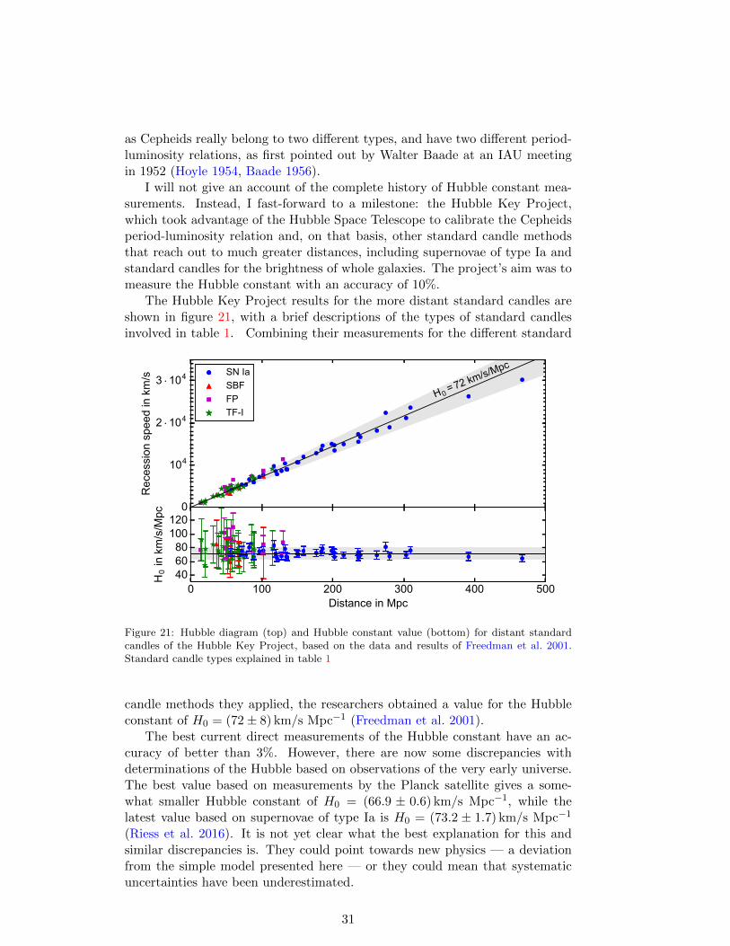
The Hubble Key Project results for the more distant standard candles areshown in figure 21, with a brief descriptions of the types of standard candlesinvolved in table 1. Combining their measurements for the different standard

0

104

2 104

3 104

Rec

essi

on s

peed

in k

m/s

H 0 = 72 km/s/MpcSN IaSBFFPTF-I

0 100 200 300 400 500Distance in Mpc

406080

100120

H0

in k

m/s

/Mpc

Figure 21: Hubble diagram (top) and Hubble constant value (bottom) for distant standardcandles of the Hubble Key Project, based on the data and results of Freedman et al. 2001.Standard candle types explained in table 1

candle methods they applied, the researchers obtained a value for the Hubbleconstant of H0 = (72± 8) km/s Mpc−1 (Freedman et al. 2001).

The best current direct measurements of the Hubble constant have an ac-curacy of better than 3%. However, there are now some discrepancies withdeterminations of the Hubble based on observations of the very early universe.The best value based on measurements by the Planck satellite gives a some-what smaller Hubble constant of H0 = (66.9 ± 0.6) km/s Mpc−1, while thelatest value based on supernovae of type Ia is H0 = (73.2 ± 1.7) km/s Mpc−1

(Riess et al. 2016). It is not yet clear what the best explanation for this andsimilar discrepancies is. They could point towards new physics — a deviationfrom the simple model presented here — or they could mean that systematicuncertainties have been underestimated.

31

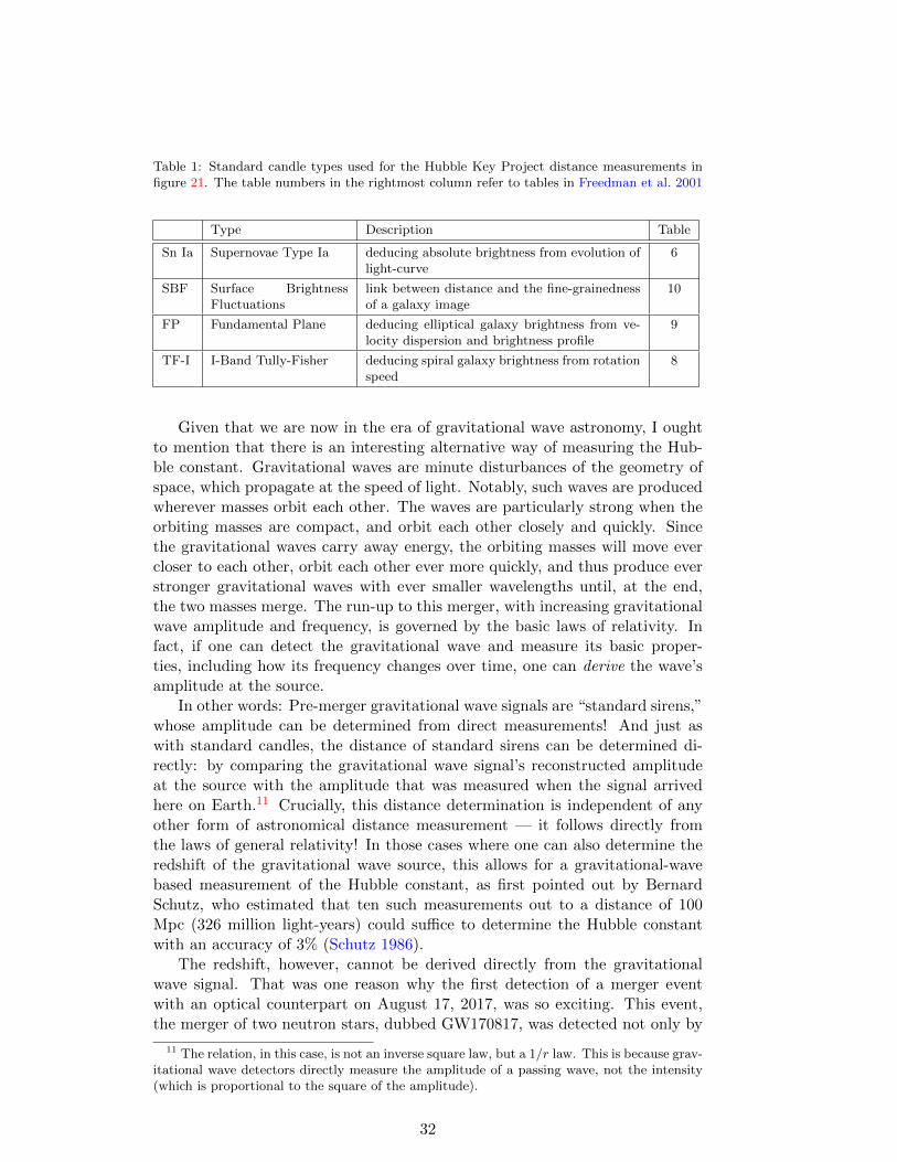
Table 1: Standard candle types used for the Hubble Key Project distance measurements infigure 21. The table numbers in the rightmost column refer to tables in Freedman et al. 2001

Type Description Table

Sn Ia Supernovae Type Ia deducing absolute brightness from evolution oflight-curve

6

SBF Surface BrightnessFluctuations

link between distance and the fine-grainednessof a galaxy image

10

FP Fundamental Plane deducing elliptical galaxy brightness from ve-locity dispersion and brightness profile

9

TF-I I-Band Tully-Fisher deducing spiral galaxy brightness from rotationspeed

8

Given that we are now in the era of gravitational wave astronomy, I oughtto mention that there is an interesting alternative way of measuring the Hub-ble constant. Gravitational waves are minute disturbances of the geometry ofspace, which propagate at the speed of light. Notably, such waves are producedwherever masses orbit each other. The waves are particularly strong when theorbiting masses are compact, and orbit each other closely and quickly. Sincethe gravitational waves carry away energy, the orbiting masses will move evercloser to each other, orbit each other ever more quickly, and thus produce everstronger gravitational waves with ever smaller wavelengths until, at the end,the two masses merge. The run-up to this merger, with increasing gravitationalwave amplitude and frequency, is governed by the basic laws of relativity. Infact, if one can detect the gravitational wave and measure its basic proper-ties, including how its frequency changes over time, one can derive the wave’samplitude at the source.

In other words: Pre-merger gravitational wave signals are “standard sirens,”whose amplitude can be determined from direct measurements! And just aswith standard candles, the distance of standard sirens can be determined di-rectly: by comparing the gravitational wave signal’s reconstructed amplitudeat the source with the amplitude that was measured when the signal arrivedhere on Earth.11 Crucially, this distance determination is independent of anyother form of astronomical distance measurement — it follows directly fromthe laws of general relativity! In those cases where one can also determine theredshift of the gravitational wave source, this allows for a gravitational-wavebased measurement of the Hubble constant, as first pointed out by BernardSchutz, who estimated that ten such measurements out to a distance of 100Mpc (326 million light-years) could suffice to determine the Hubble constantwith an accuracy of 3% (Schutz 1986).

The redshift, however, cannot be derived directly from the gravitationalwave signal. That was one reason why the first detection of a merger eventwith an optical counterpart on August 17, 2017, was so exciting. This event,the merger of two neutron stars, dubbed GW170817, was detected not only by

11 The relation, in this case, is not an inverse square law, but a 1/r law. This is because grav-itational wave detectors directly measure the amplitude of a passing wave, not the intensity(which is proportional to the square of the amplitude).

32

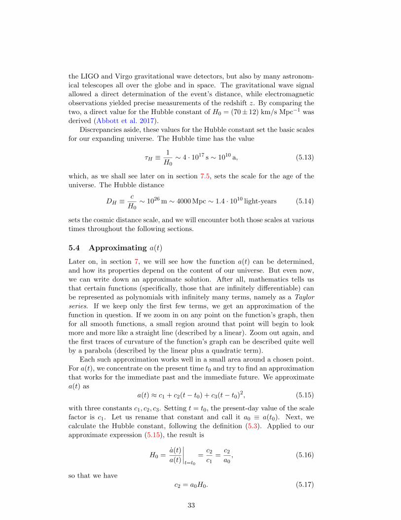
the LIGO and Virgo gravitational wave detectors, but also by many astronom-ical telescopes all over the globe and in space. The gravitational wave signalallowed a direct determination of the event’s distance, while electromagneticobservations yielded precise measurements of the redshift z. By comparing thetwo, a direct value for the Hubble constant of H0 = (70± 12) km/s Mpc−1 wasderived (Abbott et al. 2017).

Discrepancies aside, these values for the Hubble constant set the basic scalesfor our expanding universe. The Hubble time has the value

τH ≡1

H0∼ 4 · 1017 s ∼ 1010 a, (5.13)

which, as we shall see later on in section 7.5, sets the scale for the age of theuniverse. The Hubble distance

DH ≡c

H0∼ 1026 m ∼ 4000 Mpc ∼ 1.4 · 1010 light-years (5.14)

sets the cosmic distance scale, and we will encounter both those scales at varioustimes throughout the following sections.

5.4 Approximating a(t)

Later on, in section 7, we will see how the function a(t) can be determined,and how its properties depend on the content of our universe. But even now,we can write down an approximate solution. After all, mathematics tells usthat certain functions (specifically, those that are infinitely differentiable) canbe represented as polynomials with infinitely many terms, namely as a Taylorseries. If we keep only the first few terms, we get an approximation of thefunction in question. If we zoom in on any point on the function’s graph, thenfor all smooth functions, a small region around that point will begin to lookmore and more like a straight line (described by a linear). Zoom out again, andthe first traces of curvature of the function’s graph can be described quite wellby a parabola (described by the linear plus a quadratic term).

Each such approximation works well in a small area around a chosen point.For a(t), we concentrate on the present time t0 and try to find an approximationthat works for the immediate past and the immediate future. We approximatea(t) as

a(t) ≈ c1 + c2(t− t0) + c3(t− t0)2, (5.15)

with three constants c1, c2, c3. Setting t = t0, the present-day value of the scalefactor is c1. Let us rename that constant and call it a0 ≡ a(t0). Next, wecalculate the Hubble constant, following the definition (5.3). Applied to ourapproximate expression (5.15), the result is

H0 =a(t)

a(t)

∣∣∣∣t=t0

=c2

c1=c2

a0, (5.16)

so that we havec2 = a0H0. (5.17)

33

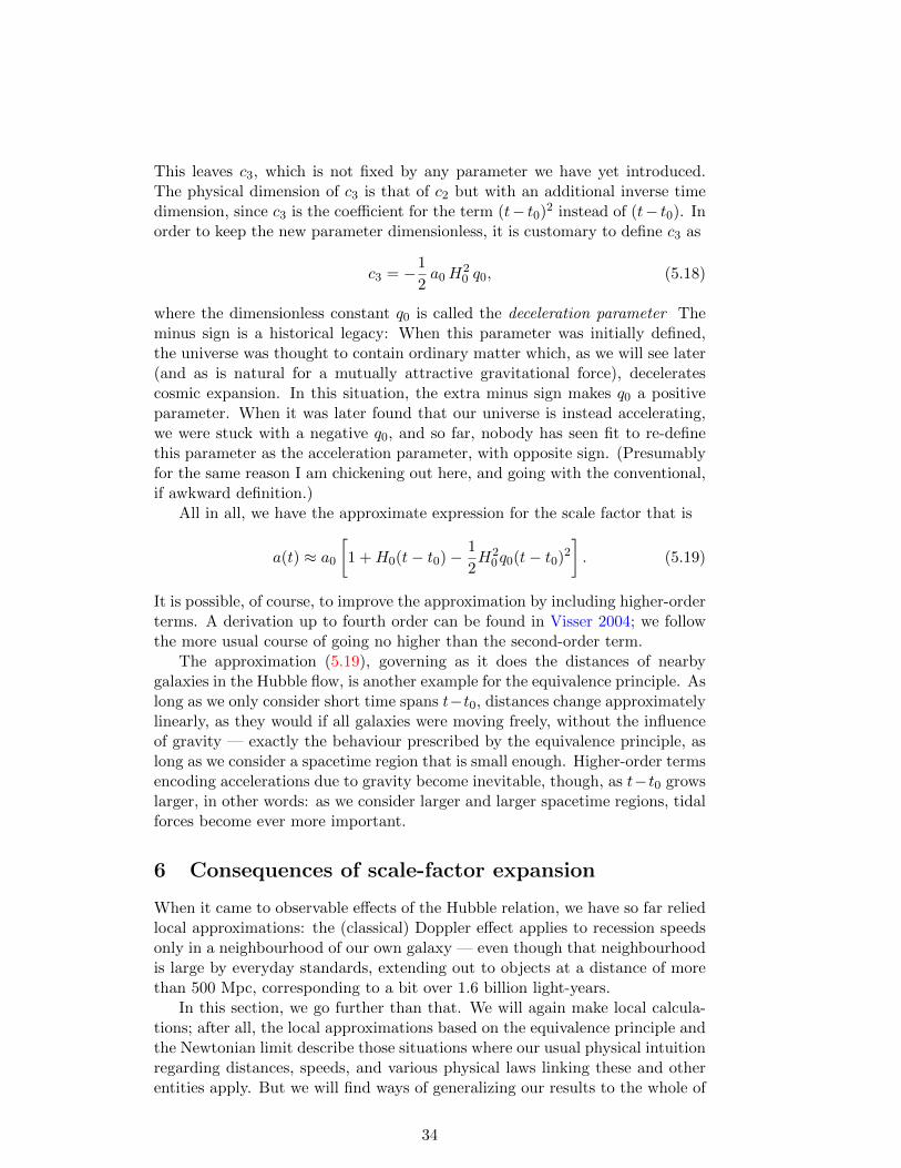
This leaves c3, which is not fixed by any parameter we have yet introduced.The physical dimension of c3 is that of c2 but with an additional inverse timedimension, since c3 is the coefficient for the term (t− t0)2 instead of (t− t0). Inorder to keep the new parameter dimensionless, it is customary to define c3 as

c3 = −1

2a0H

20 q0, (5.18)

where the dimensionless constant q0 is called the deceleration parameter Theminus sign is a historical legacy: When this parameter was initially defined,the universe was thought to contain ordinary matter which, as we will see later(and as is natural for a mutually attractive gravitational force), deceleratescosmic expansion. In this situation, the extra minus sign makes q0 a positiveparameter. When it was later found that our universe is instead accelerating,we were stuck with a negative q0, and so far, nobody has seen fit to re-definethis parameter as the acceleration parameter, with opposite sign. (Presumablyfor the same reason I am chickening out here, and going with the conventional,if awkward definition.)

All in all, we have the approximate expression for the scale factor that is

a(t) ≈ a0

[1 +H0(t− t0)− 1

2H2

0q0(t− t0)2

]. (5.19)

It is possible, of course, to improve the approximation by including higher-orderterms. A derivation up to fourth order can be found in Visser 2004; we followthe more usual course of going no higher than the second-order term.

The approximation (5.19), governing as it does the distances of nearbygalaxies in the Hubble flow, is another example for the equivalence principle. Aslong as we only consider short time spans t−t0, distances change approximatelylinearly, as they would if all galaxies were moving freely, without the influenceof gravity — exactly the behaviour prescribed by the equivalence principle, aslong as we consider a spacetime region that is small enough. Higher-order termsencoding accelerations due to gravity become inevitable, though, as t−t0 growslarger, in other words: as we consider larger and larger spacetime regions, tidalforces become ever more important.

6 Consequences of scale-factor expansion

When it came to observable effects of the Hubble relation, we have so far reliedlocal approximations: the (classical) Doppler effect applies to recession speedsonly in a neighbourhood of our own galaxy — even though that neighbourhoodis large by everyday standards, extending out to objects at a distance of morethan 500 Mpc, corresponding to a bit over 1.6 billion light-years.

In this section, we go further than that. We will again make local calcula-tions; after all, the local approximations based on the equivalence principle andthe Newtonian limit describe those situations where our usual physical intuitionregarding distances, speeds, and various physical laws linking these and otherentities apply. But we will find ways of generalizing our results to the whole of

34

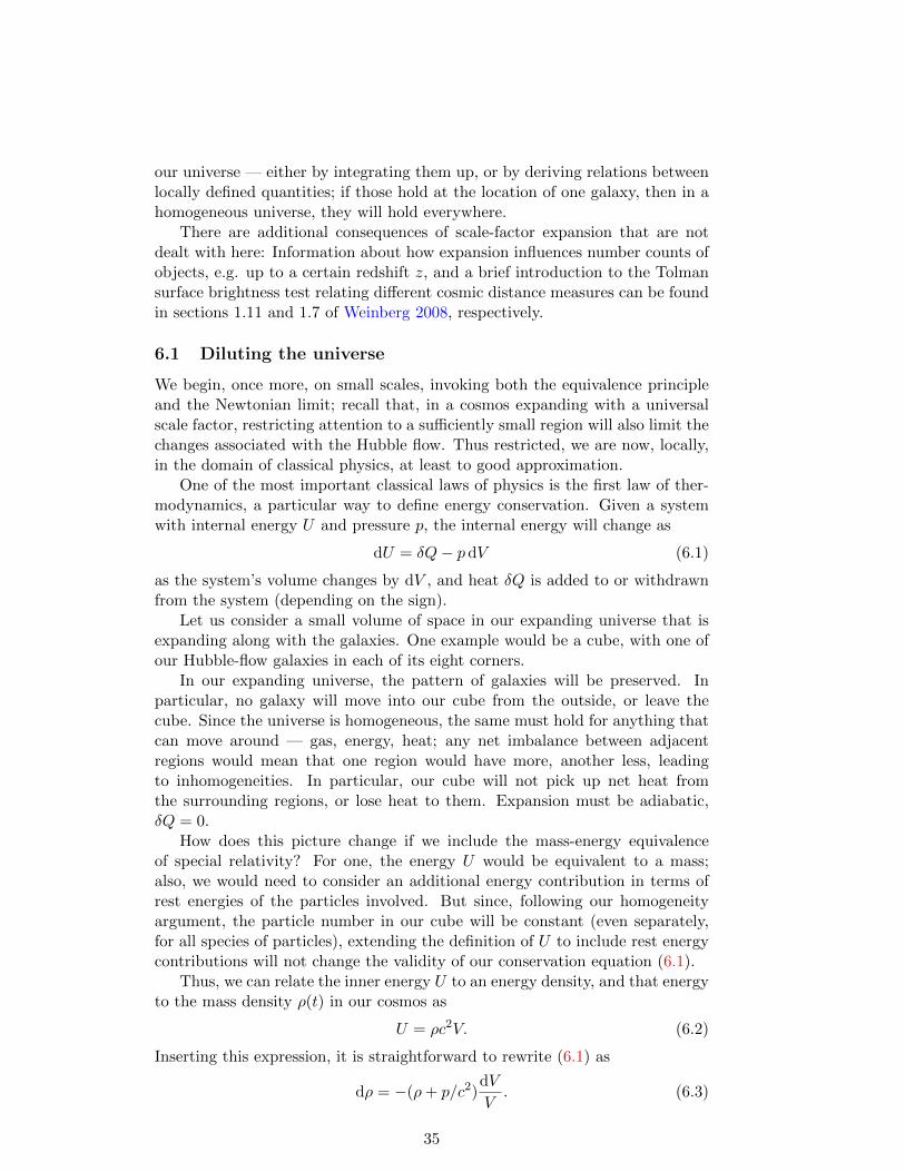
our universe — either by integrating them up, or by deriving relations betweenlocally defined quantities; if those hold at the location of one galaxy, then in ahomogeneous universe, they will hold everywhere.

There are additional consequences of scale-factor expansion that are notdealt with here: Information about how expansion influences number counts ofobjects, e.g. up to a certain redshift z, and a brief introduction to the Tolmansurface brightness test relating different cosmic distance measures can be foundin sections 1.11 and 1.7 of Weinberg 2008, respectively.

6.1 Diluting the universe

We begin, once more, on small scales, invoking both the equivalence principleand the Newtonian limit; recall that, in a cosmos expanding with a universalscale factor, restricting attention to a sufficiently small region will also limit thechanges associated with the Hubble flow. Thus restricted, we are now, locally,in the domain of classical physics, at least to good approximation.

One of the most important classical laws of physics is the first law of ther-modynamics, a particular way to define energy conservation. Given a systemwith internal energy U and pressure p, the internal energy will change as

dU = δQ− p dV (6.1)

as the system’s volume changes by dV , and heat δQ is added to or withdrawnfrom the system (depending on the sign).

Let us consider a small volume of space in our expanding universe that isexpanding along with the galaxies. One example would be a cube, with one ofour Hubble-flow galaxies in each of its eight corners.

In our expanding universe, the pattern of galaxies will be preserved. Inparticular, no galaxy will move into our cube from the outside, or leave thecube. Since the universe is homogeneous, the same must hold for anything thatcan move around — gas, energy, heat; any net imbalance between adjacentregions would mean that one region would have more, another less, leadingto inhomogeneities. In particular, our cube will not pick up net heat fromthe surrounding regions, or lose heat to them. Expansion must be adiabatic,δQ = 0.

How does this picture change if we include the mass-energy equivalenceof special relativity? For one, the energy U would be equivalent to a mass;also, we would need to consider an additional energy contribution in terms ofrest energies of the particles involved. But since, following our homogeneityargument, the particle number in our cube will be constant (even separately,for all species of particles), extending the definition of U to include rest energycontributions will not change the validity of our conservation equation (6.1).

Thus, we can relate the inner energy U to an energy density, and that energyto the mass density ρ(t) in our cosmos as

U = ρc2V. (6.2)

Inserting this expression, it is straightforward to rewrite (6.1) as

dρ = −(ρ+ p/c2)dV

V. (6.3)

35

Recall that we are not considering an arbitrary volume, but one that is linkedto cosmic expansion. If all lengths scale ∼ a(t), then any volume will scale∼ a(t)3. This is easily seen in the case of a cube, where the volume is the cubeof the side length, and the side length scales with a(t).

In consequence, the volume changes as

V (t) =

(a(t)

a(t0)

)3

V (t0), (6.4)

so the differential change in volume, dV , corresponding to a small change da inthe scale factor, is

dV

V= 3

da

a. (6.5)

Insert this into (6.3) and you get the differential change in density, dρ, corre-sponding to the small scale factor change, namely

dρ = −3(ρ+ p/c2)da

a. (6.6)

A special case of this is how densities change with cosmic time,

ρ = −3(ρ+ p/c2)a

a= −3(ρ+ p/c2) H(t). (6.7)

This depends on two quantities describing the state of cosmic matter: the(mass) density ρ and the pressure p. In order to find a solution to this equation,we will need additional information: we will need to know how density andpressure are related. This information is encapsulated in what is called theequation of state of the matter in question, p = p(ρ).

In cosmology, it is usual to consider different equations of state, all of whichare of the form

p = w · ρc2 (6.8)

for some specific constant w:

Matter (“galaxy dust”): p = 0, w = 0

Electromagnetic radiation: p = ρc2/3, w = 13

Dark energy (scalar field): p = −ρc2, w = −1.

Matter, in this particular context, refers to our “galaxy dust” of galaxy pointparticles. In a local frame, the speed values for such galaxies are much slowerthan the speed of light, and their momentum values much smaller than theirenergy divided by c. That is why it is an excellent approximation to set thepressure to zero, p = 0.

For electromagnetic radiation filling an expanding universe — for instancein the form of thermal radiation — we can make no such approximation. FromMaxwell’s theory, physicists know, and have known for some time (Maxwell1873, §792), that radiation pressure and radiation energy density ρE are linkedas p = ρE/3.

36

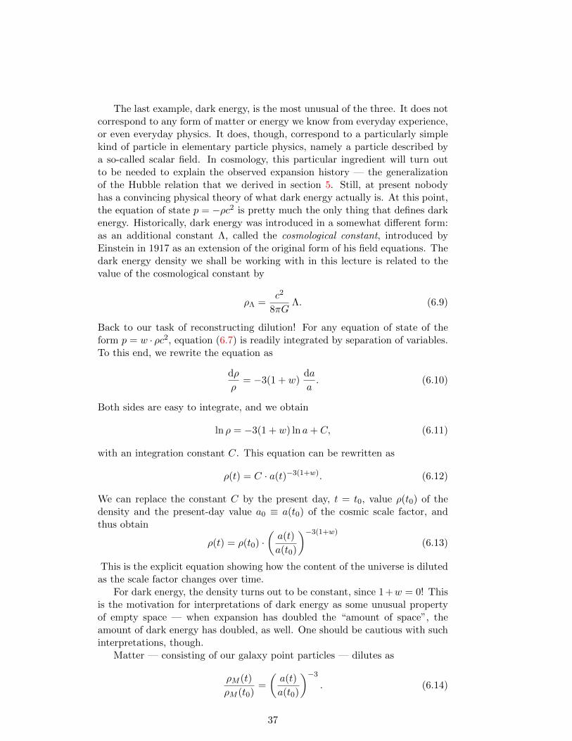
The last example, dark energy, is the most unusual of the three. It does notcorrespond to any form of matter or energy we know from everyday experience,or even everyday physics. It does, though, correspond to a particularly simplekind of particle in elementary particle physics, namely a particle described bya so-called scalar field. In cosmology, this particular ingredient will turn outto be needed to explain the observed expansion history — the generalizationof the Hubble relation that we derived in section 5. Still, at present nobodyhas a convincing physical theory of what dark energy actually is. At this point,the equation of state p = −ρc2 is pretty much the only thing that defines darkenergy. Historically, dark energy was introduced in a somewhat different form:as an additional constant Λ, called the cosmological constant, introduced byEinstein in 1917 as an extension of the original form of his field equations. Thedark energy density we shall be working with in this lecture is related to thevalue of the cosmological constant by

ρΛ =c2

8πGΛ. (6.9)

Back to our task of reconstructing dilution! For any equation of state of theform p = w · ρc2, equation (6.7) is readily integrated by separation of variables.To this end, we rewrite the equation as

dρ

ρ= −3(1 + w)

da

a. (6.10)

Both sides are easy to integrate, and we obtain

ln ρ = −3(1 + w) ln a+ C, (6.11)

with an integration constant C. This equation can be rewritten as

ρ(t) = C · a(t)−3(1+w). (6.12)

We can replace the constant C by the present day, t = t0, value ρ(t0) of thedensity and the present-day value a0 ≡ a(t0) of the cosmic scale factor, andthus obtain

ρ(t) = ρ(t0) ·(a(t)

a(t0)

)−3(1+w)

(6.13)

This is the explicit equation showing how the content of the universe is dilutedas the scale factor changes over time.

For dark energy, the density turns out to be constant, since 1 +w = 0! Thisis the motivation for interpretations of dark energy as some unusual propertyof empty space — when expansion has doubled the “amount of space”, theamount of dark energy has doubled, as well. One should be cautious with suchinterpretations, though.

Matter — consisting of our galaxy point particles — dilutes as

ρM (t)

ρM (t0)=

(a(t)

a(t0)

)−3

. (6.14)

37

This is as expected: the number of galaxies within our “co-moving cube” re-mains constant, since the pattern inside the cube, defined by the galaxies andtheir locations, remains the same; each galaxy’s mass remains unchanged, sothe total mass due to galaxies inside the cube remains unchanged. On the otherhand, as we have seen, volume scales as V ∼ a3, so the density should indeedscale ∼ a−3.

While this is not surprising, it is always good to have a cross-check toperform. The next case, that of electromagnetic radiation, is more illuminating(no pun intended).

6.2 Redshifting photons

The mass density ρR of electromagnetic radiation, with its equation of statep = ρc2/3, scales as

ρR(t)

ρR(t0)=

(a(t)

a(t0)

)−4

. (6.15)

What does that tell us about light? The easiest way to answer this is to re-member that light is a mixture of light particles, called photons:

Each photon has a frequency ν and wavelength λ, with an energy E = hν =hc/λ where h is Planck’s constant, and photons travel at the vacuum speed oflight c. Photons behave like particles, and we will take that to include thatthey do not vanish suddenly, or pop into existence.

The mass density of a bunch of photons is proportional to their energydensity, and that is proportional to the sum of all the energy contributionsfrom the various photons. As space expands, the same number of photonsspread out over a larger volume V ∼ a3. If that were all, we would expect thephoton mass density to vary as ρ ∼ a−3. The extra factor a−1 must mean thatthe energies of all the separate photons decrease with time, as well, as E ∼ a−1.

Given that for these photon energies, E = hc/λ, this means that eachphoton wavelength gets stretched in proportion to a(t), namely as

λ(t) = λ0 ·a(t)

a(t0). (6.16)

This is an alternative form of the cosmological redshift we had encounteredas an approximate Doppler shift in section 5.1: photon wavelengths increase inproportion to the universal scale factor, just like the distances between galaxiesin the Hubble flow.

There are some aspects of this derivation one might well be skeptical about.Is photon number really conserved, or is that taking our physical intuition too

38

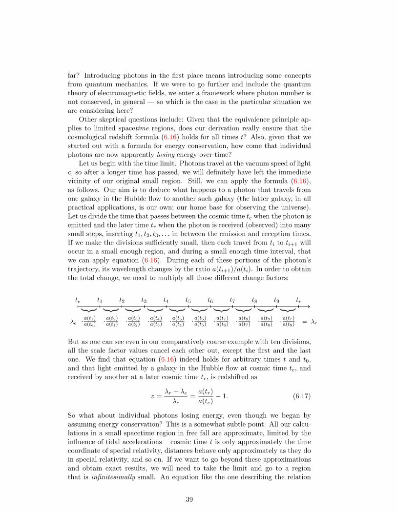
far? Introducing photons in the first place means introducing some conceptsfrom quantum mechanics. If we were to go further and include the quantumtheory of electromagnetic fields, we enter a framework where photon number isnot conserved, in general — so which is the case in the particular situation weare considering here?

Other skeptical questions include: Given that the equivalence principle ap-plies to limited spacetime regions, does our derivation really ensure that thecosmological redshift formula (6.16) holds for all times t? Also, given that westarted out with a formula for energy conservation, how come that individualphotons are now apparently losing energy over time?

Let us begin with the time limit. Photons travel at the vacuum speed of lightc, so after a longer time has passed, we will definitely have left the immediatevicinity of our original small region. Still, we can apply the formula (6.16),as follows. Our aim is to deduce what happens to a photon that travels fromone galaxy in the Hubble flow to another such galaxy (the latter galaxy, in allpractical applications, is our own; our home base for observing the universe).Let us divide the time that passes between the cosmic time te when the photon isemitted and the later time tr when the photon is received (observed) into manysmall steps, inserting t1, t2, t3, . . . in between the emission and reception times.If we make the divisions sufficiently small, then each travel from ti to ti+1 willoccur in a small enough region, and during a small enough time interval, thatwe can apply equation (6.16). During each of these portions of the photon’strajectory, its wavelength changes by the ratio a(ti+1)/a(ti). In order to obtainthe total change, we need to multiply all those different change factors:

t1 t2 t3 t4 t5 t6 t7 t8 t9

·a(t2)a(t1) ·a(t3)

a(t2) ·a(t4)a(t3) ·a(t5)

a(t4) ·a(t6)a(t5) ·a(t7)

a(t6) ·a(t8)a(t7) ·a(t9)

a(t8)

︸ ︷︷ ︸ ︸ ︷︷ ︸ ︸ ︷︷ ︸ ︸ ︷︷ ︸ ︸ ︷︷ ︸ ︸ ︷︷ ︸ ︸ ︷︷ ︸ ︸ ︷︷ ︸ ︸ ︷︷ ︸ ︸ ︷︷ ︸te tr

·a(t1)a(te) ·a(tr)

a(t9)λe = λr

But as one can see even in our comparatively coarse example with ten divisions,all the scale factor values cancel each other out, except the first and the lastone. We find that equation (6.16) indeed holds for arbitrary times t and t0,and that light emitted by a galaxy in the Hubble flow at cosmic time te, andreceived by another at a later cosmic time tr, is redshifted as

z =λr − λeλe

=a(tr)

a(te)− 1. (6.17)

So what about individual photons losing energy, even though we began byassuming energy conservation? This is a somewhat subtle point. All our calcu-lations in a small spacetime region in free fall are approximate, limited by theinfluence of tidal accelerations – cosmic time t is only approximately the timecoordinate of special relativity, distances behave only approximately as they doin special relativity, and so on. If we want to go beyond these approximationsand obtain exact results, we will need to take the limit and go to a regionthat is infinitesimally small. An equation like the one describing the relation

39

between the density and the scale factor, equation (6.13), remains valid in thatinfinitesimal limit, since the density of an infinitesimally region is well-defined— which is why, in an inhomogeneous situation, we are able to talk about thedensity of a continuum at a specific location.

But an equation like the one we have just derived for the redshift of aphoton, (6.17), is not preserved if we go to the infinitesimal limit. The limitof restricting ourselves to an infinitesimal region, tr → te, is the limit wherez → 0, that is, where the photon is not redshifted at all. Equation (6.17), asit stands, describes a non-infinitesimal region. Which is fine, but it also meansthat we have to face up to cosmic time t being an unusual coordinate. The twogalaxies emitting and receiving the light are not at rest relative to each other,yet cosmic time links their proper time coordinates to create the global timecoordinate we call cosmic time. And for galaxies that are not at rest relativeto each other, there will be a Doppler shift.

In special relativity, when light is emitted by an observer, and received byan observer who is in motion relative to the first, of course the second observerwill measure a different wavelength, and thus energy, for each individual photon(cf. the brief account of the Doppler effect in special relativity in section B.5).In that situation, we would never wonder how the photon in question had “lost”or “gained” energy. We would see quite clearly what had happened, namelythat we are dealing with more than one frame of reference. The initial energywas measured in one inertial frame, and the receiver was in another inertialframe. Emitter and receiver are in relative motion; hence, the Doppler effectand the fact that the receiver measures a different energy.

In our cosmological situation, we know that at least in the small-region ap-proximation, our galaxies are in motion; at large scales, we know that cosmictime t is not an ordinary, special-relativistic time coordinate, but somethingmore unusual. Given those two circumstances, even with our rather limitedunderstanding, the most parsimonious explanation is that the apparent loss ofphoton energy is due to the fact that emitter and receiver are in relative motion,or in what passes for relative motion in the more general framework of an ex-panding universe. A more thorough examination, including a generalization ofthe special-relativistic notion of relative speed by introducing a concept knownas parallel transport, confirms this (Narlikar 1994, Bunn and Hogg 2009).

Still, with the remaining doubts about photon number conservation, and thequestion of whether or not equation (6.17) remains valid beyond the (trivial)infinitesimal limit z → 0, it makes sense for us to look at a more rigorousderivation of how photons propagate, and are redshifted.

6.3 Light propagation in an expanding universe

Consider the propagation of light that was emitted by one galaxy at time te, andreceived in another galaxy at a later time tr. We think of light as a point-likepulse with a well-defined location at each moment in time, and follow the samestrategy as before: We make our calculations locally, in freely falling systems,considering only a small spacetime region for each and exploiting the fact thatcosmic time t is an inertial coordinate there, at least approximately. A similar

40

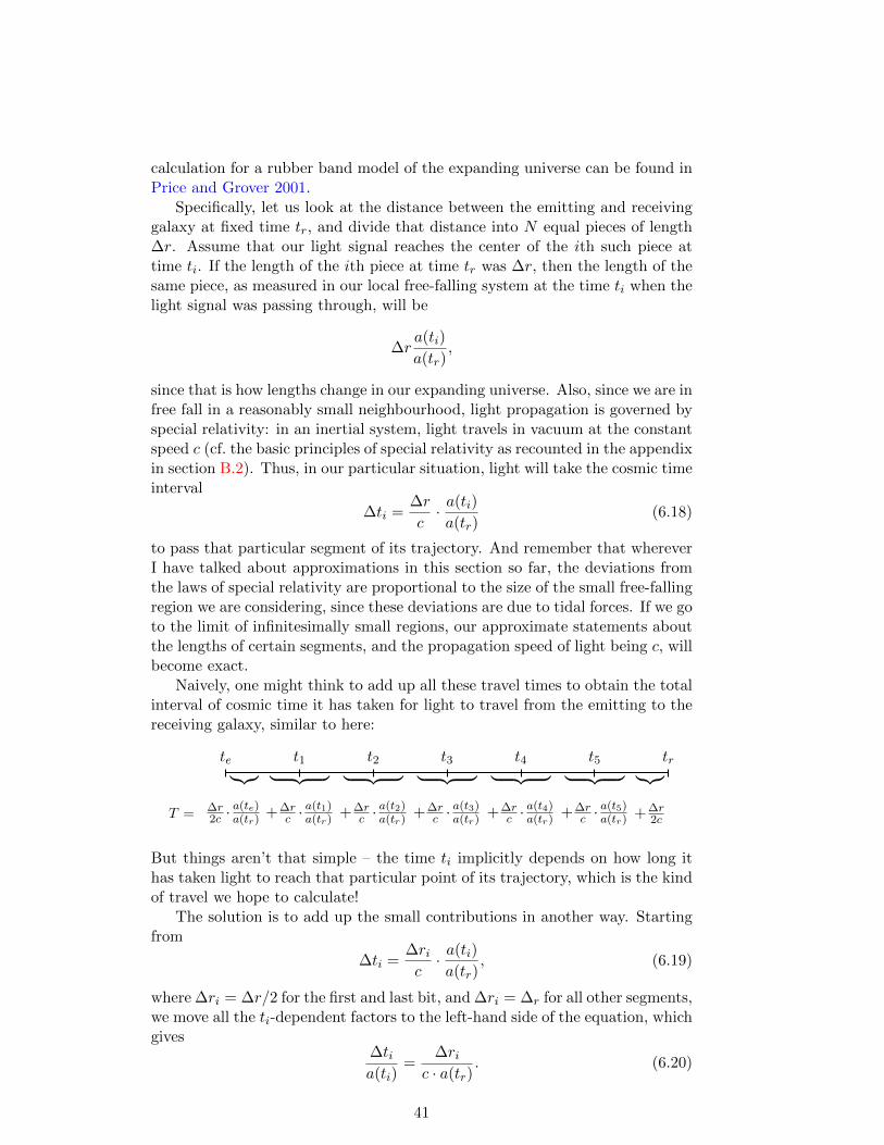
calculation for a rubber band model of the expanding universe can be found inPrice and Grover 2001.

Specifically, let us look at the distance between the emitting and receivinggalaxy at fixed time tr, and divide that distance into N equal pieces of length∆r. Assume that our light signal reaches the center of the ith such piece attime ti. If the length of the ith piece at time tr was ∆r, then the length of thesame piece, as measured in our local free-falling system at the time ti when thelight signal was passing through, will be

∆ra(ti)

a(tr),

since that is how lengths change in our expanding universe. Also, since we are infree fall in a reasonably small neighbourhood, light propagation is governed byspecial relativity: in an inertial system, light travels in vacuum at the constantspeed c (cf. the basic principles of special relativity as recounted in the appendixin section B.2). Thus, in our particular situation, light will take the cosmic timeinterval

∆ti =∆r

c· a(ti)

a(tr)(6.18)

to pass that particular segment of its trajectory. And remember that whereverI have talked about approximations in this section so far, the deviations fromthe laws of special relativity are proportional to the size of the small free-fallingregion we are considering, since these deviations are due to tidal forces. If we goto the limit of infinitesimally small regions, our approximate statements aboutthe lengths of certain segments, and the propagation speed of light being c, willbecome exact.

Naively, one might think to add up all these travel times to obtain the totalinterval of cosmic time it has taken for light to travel from the emitting to thereceiving galaxy, similar to here:

t1 t2 t3 t4 t5

+∆rc ·

a(t1)a(tr) +∆r

c ·a(t2)a(tr) +∆r

c ·a(t3)a(tr) +∆r

c ·a(t4)a(tr) +∆r

c ·a(t5)a(tr)

︸ ︷︷ ︸ ︸ ︷︷ ︸ ︸ ︷︷ ︸ ︸ ︷︷ ︸ ︸ ︷︷ ︸te tr

∆r2c ·

a(te)a(tr) +∆r

2cT =

︸︷︷︸ ︸︷︷︸

But things aren’t that simple – the time ti implicitly depends on how long ithas taken light to reach that particular point of its trajectory, which is the kindof travel we hope to calculate!

The solution is to add up the small contributions in another way. Startingfrom

∆ti =∆ric· a(ti)

a(tr), (6.19)

where ∆ri = ∆r/2 for the first and last bit, and ∆ri = ∆r for all other segments,we move all the ti-dependent factors to the left-hand side of the equation, whichgives

∆tia(ti)

=∆ri

c · a(tr). (6.20)

41

Summing over all the segments involved, we get

N∑i=1

∆tia(ti)

=1

c · a(tr)dr,e(tr), (6.21)

where on the right-hand side we have used the fact that, by definition, thelength segments add up to the distance of the emitting and receiving galaxiesat the time tr of reception.

If we make N infinitely large, and our segments infinitesimally small, theleft-hand side becomes an integral, and we end up with12

dr,e(tr) = c · a(tr) ·tr∫te

dt

a(t). (6.22)

This is the key equation for light propagation in an expanding universe, linkinglight travel time tr − te to the distance dr,e(tr) at the time of reception. Ofcourse, in order to evaluate the integral, we will need the explicit form of theuniversal scale factor as a function of cosmic time, a(t). This requires additionalcalculations, which I will present in section 7.

For signals we receive at the present time, tr = t0, it is again straightforwardto see how this distance is related to the look-back time if we consider our seriesexpansion for a(t) given in equation (5.19). Inserting that approximation, wehave

dr,e(t0) = c ·t0∫te

dt

1 +H0(t− t0)− 12H

20q0(t− t0)2

. (6.23)

We can simplify this integral in two ways. For the denominator, we make useof the geometric series approximation

1

1 +X= 1−X + . . . ; (6.24)

this formula gives a good approximation whenever X is small, in our case:whenever t0 − t is considerably smaller than the Hubble time τH = 1/H0.In addition, we choose another integration variable, namely t′ = t0 − t. Ourexpression for the distance then becomes

dr,e(t0) = c ·t0−te∫0

dt′

1−H0t′ − 12H

20q0(t′)2

≈ c ·t0−te∫0

dt′(1 +H0t

′)= c(t0 − te) +

1

2cH0(t0 − te)2, (6.25)

where we have again only kept terms up to second order. This expression showsthat, at least for shorter distances, the proper distance dr,e is approximately

12Why does this appear to have a minus sign, compared to the usual derivation using themetric and radial coordinate? Because with the radial coordinate, we specifically look at lighttravelling inwards towards smaller radius values, so rr − re is equal to minus the comovingdistance.

42

equal to the look-back time t0−te times the usual vacuum speed of light, just asin special relativity. For larger distances, and thus larger look-back times t0−te,additional effects come into play, and the relation becomes more complicated.

In fact, the look-back time, as the time it takes light from a distant objectto reach us, is one possible definition of a distance in an expanding universe.Our formula shows that for smaller distance values, the look-back time and theproper distance dr,e are approximately the same, while for larger distances, thetwo definitions diverge.

6.4 Cosmological redshift revisited

Even though we do not yet have the knowledge to find explicit solutions to thelight propagation equation (6.22), since we do not yet know the explicit formof a(t), there are some conclusions we can draw already. Imagine two lightsignals leaving a distant galaxy at r = re at consecutive cosmic times te andte + δte, arriving at a second galaxy at time tr and tr + δtr. Then by our lightpropagation equation (6.22), we have

tr∫te

c dt

a(t)=dr,e(tr)

a(tr)and

tr+δtr∫te+δte

c dt

a(t)=dr,e(tr + δtr)

a(tr + δtr). (6.26)

But the expressions on the right-hand sides of these two equations are thesame — after all, that is how distances change in a universe expanding with auniversal scale factors, cf. equation (4.1). That means we have tr+δtr∫

te+δte

−tr∫te

c dt

a(t)= 0, (6.27)

or, exploiting the facts that we can split integration ranges into separate seg-ments, and combine adjacent segments, and that an integral changes sign if youreverse upper and lower limit,13 tr+δtr∫

tr

+

tr∫te+δte

−tr∫te

c dt

a(t)=

tr+δtr∫tr

−te+δte∫tr

−tr∫te

c dt

a(t)

=

tr+δtr∫tr

−te+δte∫te

c dt

a(t)= 0. (6.28)

13 Written out, this means that we have additivity,

b∫a

f(x)dx =

c∫a

f(x)dx+

b∫c

f(x)dx,

and a sign change when we reverse the boundary values,

b∫a

f(x)dx = −a∫

b

f(x)dx.

43

However, for very small integral ranges δt, there is an approximate equality

t+δt∫t

f(t) dt ≈ f(t) · δt, (6.29)

which in our case translates to

δtra(tr)

=δtea(te)

. (6.30)

Our two light signals, one closely following the other, could be one of severalthings: real light pulses, but also consecutive crests (or troughs) of elementarylight waves of frequency f ∝ 1/δt. In the latter case, we would have

frfe

=a(te)

a(tr), (6.31)

so the wavelength of the light changes as

λrλe

=a(tr)

a(te), (6.32)

reproducing formula (6.16) for the cosmological redshift, namely

z =λr − λeλe

=a(tr)

a(te)− 1. (6.33)

Note that while there was still some approximation involved in the derivation,it is of a different kind than before. Our only assumption now, necessary forevaluating the integral as in (6.29), was that a(t) should be approximatelyconstant during the time interval between the first and the second signal (crest,trough. . . ). For all realistic a(t) we are dealing with in cosmology, with theexception of the so-called inflationary phase in the very early universe, thatapproximation is valid.

Also note that not only does the derivation in this section validate ourearlier results – it extends them: formula (6.30) is valid not only for wavecrests or troughs, but more generally for light-like signals following each other.The arrival time difference of these signals will be larger than the emission timedifference. The same will apply to all consecutive signals that carry informationabout what is happening in a distant region of the cosmos. Formula (6.30)describes not only a cosmological redshift, but, more generally, cosmologicaltime dilation. The corresponding effects have been observed in the light-curvesof more vs. less distant supernovae of type Ia (Leibundgut et al. 1996).

The most common application is the case where we receive the light of adistant object at the present time, tr = t0. In that case, we can make equation(6.33) more concrete by using the series approximation for the scale factora(t) around the present time t0 which is given in equation (5.19) in termsof the constants a0, H0, q0. In order to get everything nice and polynomial,we will again use the series approximation (6.24). The series expansion for

44

a(t) is in terms of t0 − te, called the lookback time, namely the time that haspassed between the emission of the light and us receiving it. Putting everythingtogether, we get

z ≈ H0(t0 − te) +1

2H2

0 (q0 + 2)(t0 − te)2. (6.34)

This can be inverted to give the lookback time as a polynomial of the redshiftz, again keeping only terms up to second order, namely

H0(t0 − te) ≈ z −1

2(q0 + 2)z2. (6.35)

Using this in our approximate relation (6.25) between the present-day distancedr,e(t0) and the look-back time, we can derive an approximate redshift-distancerelation, which turns out to be

dr,e(z) =c

H0

(z − 1

2(q0 + 1)z2

)= DH

(z − 1

2(q0 + 1)z2

), (6.36)

where the last expression again uses the Hubble distance DH ≡ c/H0. Theterm linear in z is the linear redshift-distance relation we had already derivedas equation (5.8), while the term that is second order in z is the lowest-ordercorrection.

6.5 Redshift drift

Consider once more the cosmological redshift formula

z(tr) =a(tr)

a(te(tr))− 1, (6.37)

here rewritten to make explicit that, given a fixed reception time and a fixeddistant galaxy in the Hubble flow, both the redshift of that galaxy’s light arriv-ing at our own location at time tr and the time at which that light was emittedare functions of tr, namely z(tr) and te(tr).

We can differentiate both sides of this equation to see how these quantitieschange as the reception time changes. The result ist

dz

dtr=

a(tr)

a(te(tr))− a(tr)

a2(te(tr))a(te(tr))

dtedtr

. (6.38)

We can replace the a-terms using the Hubble parameter H(t) defined in equa-tion (5.2), and obtain

dz

dtr=

a(tr)

a(te(tr))

[H(tr)−H(te(tr))

dtedtr

]. (6.39)

But in equation (6.30) during our derivation of the cosmic redshift formula, wesaw that the ratio of infinitesimal changes in the emission and reception timesis proportional to the ratio of scale factor values at those times,

dtedtr

=a(te(tr))

a(tr). (6.40)

45

Finally, we can make use of the redshift formula (6.37) to rewrite all scale factorratios in terms of the redshift z(tr). The result, now once more dropping theexplicit tr-dependence-notation and noting that the Hubble parameter at thereception time is the Hubble constant H0, is

H(te) = H0(1 + z)− dz

dtr. (6.41)

On the right-hand side, we have H0, which can be measured as described insection 5.3, and we have the redshift, which is straightforward to measure. Ifwe could measure the derivative, as well, and observe how the redshift of thatdistant galaxy changes a little bit over time, then using this formula, we coulddirectly reconstruct the value H(te) of the Hubble parameter at the time thelight was emitted! By performing such measurements for galaxies at differentredshifts, we could reconstruct the change of the Hubble parameter over time,and in this way, reconstruct the expansion history of the universe!

Excitingly, such measurements are just about within reach for the next gen-eration of telescope, namely 40-meter-class telescopes such as ESO’s ExtremelyLarge Telescope currently under construction in Chile. With patience, namelyinvesting 4000 hours of observing time over 20 years, the effect could be mea-sured for extremely distant cosmic clouds of hydrogen at redshifts 2 < z < 5(Liske et al. 2008).

6.6 The geometry of space

We have seen in section 5.2 how astronomers measure distances, using standardcandles and the inverse-square law (5.12). Which parts of the derivation ofthe inverse-square law needs to be changed in an expanding universe? In thelecture itself, I immediately assumed Euclidean geometry for my calculations,mentioning in passing that this does indeed turn out to be the geometry of ourparticular expanding universe. In the written version, I will be more general,although not to the extent of writing down explicit proofs. These proofs, noneof which require familiarity with the concept of a space(time) metric, can befound in chapter 26 of Schutz 2004, on which this section is largely based.

To begin with, we should be cautious when it comes to the geometry ofspace as defined by constant values of the cosmic time t. As we saw in section4.3, we should be very careful about which of the concepts of special relativity,regarding both time and space, we can legitimately apply in an expandinguniverse.

Fortunately, the fact that our simple model universe is homogeneous andisotropic restricts the possibilities to a remarkably small number, namely three.The geometric arguments are beyond the scope of this lecture, but they, too canbe formulated without recourse to the concept of a metric. The three kinds ofthree-dimensional spaces that are compatible with homogeneity and isotropy are(1) ordinary Euclidean space, (2) a spherical space that is the three-dimensionalanalogue of a two-dimensional spherical surface, and (3) a hyperbolic space thatis the three-dimensional analogue of a two-dimensional saddle-shaped surface.

46

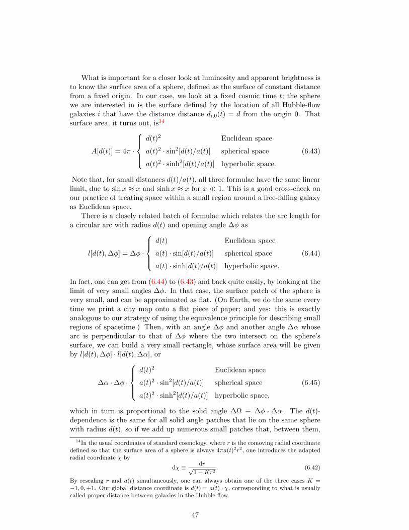
What is important for a closer look at luminosity and apparent brightness isto know the surface area of a sphere, defined as the surface of constant distancefrom a fixed origin. In our case, we look at a fixed cosmic time t; the spherewe are interested in is the surface defined by the location of all Hubble-flowgalaxies i that have the distance distance di,0(t) = d from the origin 0. Thatsurface area, it turns out, is14

A[d(t)] = 4π ·

d(t)2 Euclidean space

a(t)2 · sin2[d(t)/a(t)] spherical space

a(t)2 · sinh2[d(t)/a(t)] hyperbolic space.

(6.43)

Note that, for small distances d(t)/a(t), all three formulae have the same linearlimit, due to sinx ≈ x and sinhx ≈ x for x 1. This is a good cross-check onour practice of treating space within a small region around a free-falling galaxyas Euclidean space.

There is a closely related batch of formulae which relates the arc length fora circular arc with radius d(t) and opening angle ∆φ as

l[d(t),∆φ] = ∆φ ·

d(t) Euclidean space

a(t) · sin[d(t)/a(t)] spherical space

a(t) · sinh[d(t)/a(t)] hyperbolic space.

(6.44)

In fact, one can get from (6.44) to (6.43) and back quite easily, by looking at thelimit of very small angles ∆φ. In that case, the surface patch of the sphere isvery small, and can be approximated as flat. (On Earth, we do the same everytime we print a city map onto a flat piece of paper; and yes: this is exactlyanalogous to our strategy of using the equivalence principle for describing smallregions of spacetime.) Then, with an angle ∆φ and another angle ∆α whosearc is perpendicular to that of ∆φ where the two intersect on the sphere’ssurface, we can build a very small rectangle, whose surface area will be givenby l[d(t),∆φ] · l[d(t),∆α], or

∆α ·∆φ ·

d(t)2 Euclidean space

a(t)2 · sin2[d(t)/a(t)] spherical space

a(t)2 · sinh2[d(t)/a(t)] hyperbolic space,

(6.45)

which in turn is proportional to the solid angle ∆Ω ≡ ∆φ · ∆α. The d(t)-dependence is the same for all solid angle patches that lie on the same spherewith radius d(t), so if we add up numerous small patches that, between them,

14In the usual coordinates of standard cosmology, where r is the comoving radial coordinatedefined so that the surface area of a sphere is always 4πa(t)2r2, one introduces the adaptedradial coordinate χ by

dχ ≡ dr√1−Kr2

. (6.42)

By rescaling r and a(t) simultaneously, one can always obtain one of the three cases K =−1, 0,+1. Our global distance coordinate is d(t) = a(t) · χ, corresponding to what is usuallycalled proper distance between galaxies in the Hubble flow.

47

cover the whole sphere, the solid angle patches by themselves will add up tothe full solid angle 4π. Thus, the total area will indeed turn out to be given by(6.43).

The arc length equations (6.44) can be used to define an interesting measureof distance in cosmology, called the angular diameter distance . Assume we havetwo objects A and B in the Hubble flow, equally distant from us, separatedby a proper distance L perpendicularly to the line of sight, and that bothobjects emit light towards Earth at some past time te. The geometry at thetime of light emission is as shown in figure 22. Note that while the triangle is

A

B

LG ∆φ

Figure 22: The geometry of two Hubble-flow objects A and B, separated perpendicularly tothe line of sight by a proper distance L, emitting light towards an observer within our owngalaxy G at some past time te. The diagram shows the geometry at time te

drawn with straight lines, geometry need not be flat, and in fact, the distancedang ≡ AG = BG, the distance L and the angle ∆φ shown in the figure willnot, in general, be related following the rules governing triangles in Euclideanspace. For small angles ∆φ, the straight distance L is approximately equal tothe corresponding arc length, and for ∆φ measured in radians, we have

L = ∆φ · dang, (6.46)

For a configuration of known size L, we can measure the apparent size ∆φfrom observations and use (6.46) to derive the configuration’s angular diameterdistance dang.

Following (6.44), the angular diameter distance is related to the properdistance as

dang =

d(te) Euclidean space

a(te) · sin[d(te)/a(te)] spherical space

a(te) · sinh[d(te)/a(te)] hyperbolic space.

(6.47)

The same expression can be re-written in a different form, which we will makeuse of later. By the definition of scale factor expansion, equation (4.1), wehave d(te)/a(te) = d(t0)/a0, with proper distance and scale factor evaluatedat the present time t0. Also, the formula (6.17) for the cosmological redshiftrelates the redshift z of light received from a distant object to the scale factorvalues at the time te of emission and the time t0 of reception of the light as1 + z = a0/a(te). As a result, we have

dang =

d(t0)/(1 + z) Euclidean space

a0/(1 + z) · sin[d(t0)/a0] spherical space

a0/(1 + z) · sinh[d(t0)/a0] hyperbolic space.

(6.48)

48

The most important application of the concept of angular distance concernsmeasurements of the fluctuations in the cosmic microwave background (CMB),the radiation that reaches us from the hot, dense Big Bang phase of our uni-verse, 13.8 billion years ago. From models of the universe, one can derive amaximum size for such fluctuations, given by how far a sound wave in the earlyuniverse’s plasma can travel from the time of the Big Bang to the time thecosmic microwave radiation is set free. In that case, the radius of the corre-sponding arc segment in terms of proper distance can be calculated directly,as long as we know the cosmic time now, and the cosmic time the CMB wasproduced. The angular size of the largest fluctuations can be measured on thesky, and the proper distance of these fluctuations from us can be derived fromreconstructions of cosmic history — we can tell at what age, and at what red-shift, the cosmic microwave background was set free. The only unknown, then,is which of the three formulae in (6.47) best describes the relationship betweenthese quantities, in other words: these measurements and deductions constrainthe geometry of the universe. The evidence shows that the space of our expand-ing universe is Euclidean, within the limits of accuracy of these measurements(de Bernardis et al. 2000, Bennett et al. 2013, Planck Collaboration 2016).

6.7 Luminosity, apparent brightness, and distance

After these geometric preparations, let us return to the questions of luminosity,apparent brightness, and distance. Just as we argued in section 5.2, in anexpanding universe, light sent out isotropically from a distant source will spreadout uniformly over the surface of a sphere; when we measure that light, thefraction we capture is the ratio of our telescope area (pointed directly at thedistant source!) and the total surface area of the sphere upon which the lighthas spread out.

Consider light that was emitted at some previous time te and is just nowreaching us at the present time t0. By (6.43), we know how the sphere’s surfacearea is related to the proper distance di,0(t0) between the light source and us,the observers, evaluated at the moment our telescope receives the light.

But that is not all. Both luminosity and flux density are measured in termsof energy per unit time. In the case of an expanding universe, this quantity isaffected by the cosmological redshift, and by cosmological time dilation. Eachindividual photon will undergo a redshift, so by equation (6.16), its energy Eeat the time of emission and E0 at the time t0 of reception will be related by

E0 =a(te)

a0· Ee. (6.49)

But these photons, with the energy of each individual photon diminished, areflying towards our detector in a steady stream. In this respect, they are like thelight pulses we considered in section (6.4), and their rate of arrival is afflicted bythe cosmological redshift: the distance between one photon and the followingincreases in proportion to the universal scale factor. A stream of ne photonsper second sent out by the emitting galaxy will arrive in our telescope as a

49

diminished stream of particles, at the rate

n0 =a(te)

a0· ne. (6.50)

The relation between an object’s luminosity and its apparent brightness, de-scribed as the flux density measured by a distant observer, is given by thecombination of these three effects: the homogeneous spreading-out, individualphoton redshift and a diminution of the flux rate by cosmic time dilation. Theresult is

I =L

4π·(a(te)

a0

)2

·

d(t0)−2 Euclidean space

a−20 · sin−2[d(t0)/a0] spherical space

a−20 · sinh−2[d(t0)/a0] hyperbolic space.

(6.51)

There are several ways to simplify this expression. We can eliminate thesine/hyperbolic sine terms by using the angular distance. Also, we can re-place the scale factor ratio by the redshift z, a quantity that has the advantageof being directly observable, as per the redshift formula (6.17),

1 + z =a0

a(te). (6.52)

When we apply both simplifications, the result is

I =L

4π · d2ang(t) · (1 + z)4

. (6.53)

Motivated by the simple inverse square formula, the quantity

dL(t) ≡ dang(t) · (1 + z)2 (6.54)

is called the luminosity distance. In terms of the luminosity distance, the rela-tion simply becomes

I =L

4π dL(t)2, (6.55)

just like in an ordinary, non-expanding, Euclidean-space universe.

6.8 Luminosity distance and distance moduli

Astronomy has a traditional system of expressing apparent brightness in termsof apparent magnitude — a logarithmic system that originated at a time whenastronomers still relied chiefly on that logarithmically sensitive measuring in-strument, the human eye. The apparent magnitude m2 of an object is definedrelative to that of another object with apparent magnitude m1 via the respec-tive fluxes F2 and F1, that is, the amounts of energy received from each objectper unit time, as

m2 −m1 = −2.5 log10

(F2

F1

). (6.56)

50

Since the flux only enters as a ratio, flux densities, measured with the sametelescope, can be substituted for the fluxes. Magnitude scales typically havereference objects to define what m = 0 means, so that stand-alone apparentmagnitude values can be given.

(There is a whole area of complications that arises since real astronomicalmeasurements involve measuring not the total flux, but the flux in a certainwavelength band only, using appropriate filters. We neglect this complication;strictly speaking, we will always talk about the total flux, or bolometric flux, touse the technical term. A helpful introduction to these complications, and theso-called k correction, can be found in Hogg et al. 2002.)

The absolute magnitude M of an object is defined as that object’s apparentmagnitude m when observed from a distance of 10 pc = 32.6 light-years.

Using this definition, and applying the formula (6.54) for the luminositydistance, a distant object’s absolute magnitude M and its apparent magnitudem as measured by an observer are related by

m−M = −2.5 log10

(I(dL)

I(10 pc)

)= −2.5 log10

(10 pc

dL

)2

= 5 log10

(dL

10 pc

).

(6.57)The quantity on the right is called the distance modulus corresponding to theluminosity distance dL,

µ(dL) ≡ 5 log10

(dL

10 pc

)= 5 log10

(dL

1 Mpc

)+ 25, (6.58)

sometimes designated as DM, where the re-write in terms of Mpc is to betteraccommodate typical extragalactic distance scales.

Recall the initial diagram figure 1 we are working to understand? The yaxis represents exactly this: distance moduli for the luminosity distances of theobjects in question, derived by comparing standard candles’ known luminositiesL and measured flux intensities I.

We have already made substantial strides in understanding the original di-agram, but there is still one ingredient missing: we need to look at what deter-mines the functional form of the universal scale factor a(t).

7 Dynamics: how a(t) changes over (cosmic) time

So far, a(t) was an unknown function, and all we did was calculate variousconsequences of an expansion with a given universal scale factor a(t), or aseries approximation thereof. Now, it’s time to go a step further and lookat what determines the functional form of a(t). This involves exploring thedynamics of our expanding universe — how the matter content influences cosmicexpansion. Newtonian cosmological calculations meant as a replacement of themodels of general relativity go back to the 1930s (Milne 1934, McCrea and Milne1934, McCrea 1955). Newtonian calculations as an aid to understanding can befound in a number of text books, e.g. Rindler 1977, Harrison 2000, Lotze 2002,Weinberg 2008. There are also texts that argue (as I do in these lecture notes)

51

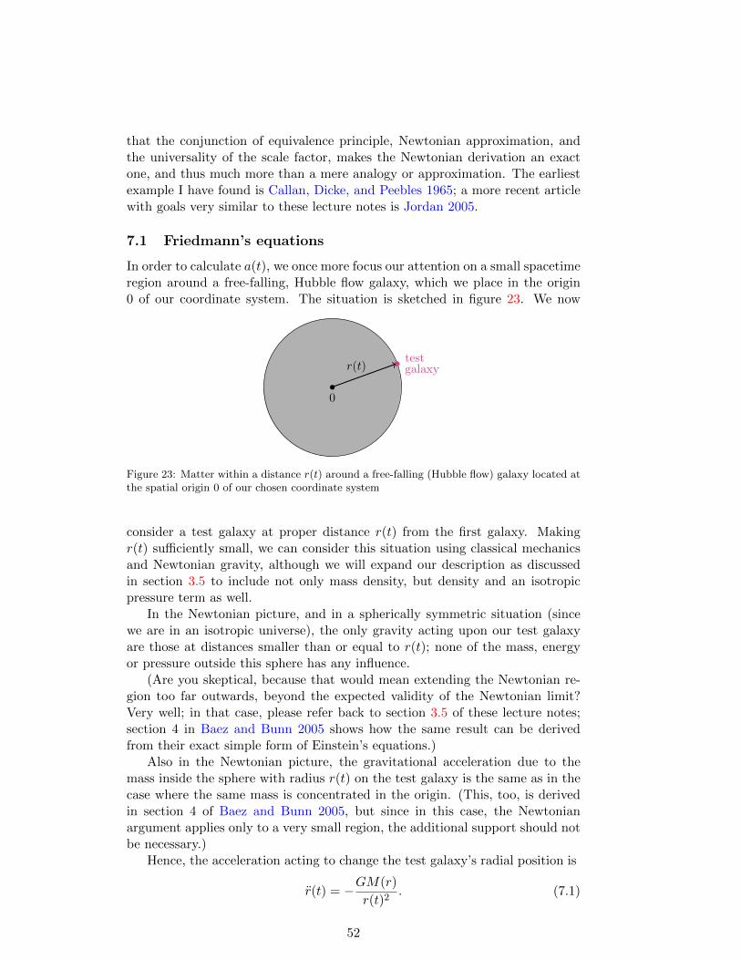
that the conjunction of equivalence principle, Newtonian approximation, andthe universality of the scale factor, makes the Newtonian derivation an exactone, and thus much more than a mere analogy or approximation. The earliestexample I have found is Callan, Dicke, and Peebles 1965; a more recent articlewith goals very similar to these lecture notes is Jordan 2005.

7.1 Friedmann’s equations

In order to calculate a(t), we once more focus our attention on a small spacetimeregion around a free-falling, Hubble flow galaxy, which we place in the origin0 of our coordinate system. The situation is sketched in figure 23. We now

testgalaxy

0

r(t)

Figure 23: Matter within a distance r(t) around a free-falling (Hubble flow) galaxy located atthe spatial origin 0 of our chosen coordinate system

consider a test galaxy at proper distance r(t) from the first galaxy. Makingr(t) sufficiently small, we can consider this situation using classical mechanicsand Newtonian gravity, although we will expand our description as discussedin section 3.5 to include not only mass density, but density and an isotropicpressure term as well.

In the Newtonian picture, and in a spherically symmetric situation (sincewe are in an isotropic universe), the only gravity acting upon our test galaxyare those at distances smaller than or equal to r(t); none of the mass, energyor pressure outside this sphere has any influence.

(Are you skeptical, because that would mean extending the Newtonian re-gion too far outwards, beyond the expected validity of the Newtonian limit?Very well; in that case, please refer back to section 3.5 of these lecture notes;section 4 in Baez and Bunn 2005 shows how the same result can be derivedfrom their exact simple form of Einstein’s equations.)

Also in the Newtonian picture, the gravitational acceleration due to themass inside the sphere with radius r(t) on the test galaxy is the same as in thecase where the same mass is concentrated in the origin. (This, too, is derivedin section 4 of Baez and Bunn 2005, but since in this case, the Newtonianargument applies only to a very small region, the additional support should notbe necessary.)

Hence, the acceleration acting to change the test galaxy’s radial position is

r(t) = −GM(r)

r(t)2. (7.1)

52

The effective mass inside the sphere is

M(r) = V (r) · (ρ+ 3p/c2), (7.2)

where V is the volume of the sphere, ρ the mass density (including contributionsfrom all available types of energy), and p the pressure, as per our discussion insection 3.5 about sources of gravity.

Since we are in a small region, geometry is approximately Euclidean, andthe volume of the sphere is given by the usual formula,

V (r) =4

3π r3, (7.3)

and since the test galaxy is in the Hubble flow, we have

r(t) =a(t)

a(t0)· r0, (7.4)

for r0 the proper radius of the sphere at some reference time t0. Putting every-thing together, it turns out that the situation-specific parameters, notably r0

and t0, cancel out, and that we are left with a second-order equation for a(t),namely

a(t)

a(t)= −4πG

3

(ρ+ 3

p

c2

). (7.5)

This is known as the second (order) Friedmann equation, after the Russiancosmologist Alexander Friedmann, the first to write down general cosmologicalmodels for an expanding universe.

Note that this is a purely local equation: We can make our region infinites-imally small and still obtain the same relation between the local quantities ρand p and the universal function a(t). Also note that while we have restrictedour attention to a small spacetime region in order to apply our equivalenceprinciple and Newtonian limit approximations, there is nothing special aboutthe cosmic time t we examined. The same reasoning can be applied to a smallspacetime region at any cosmic time, showing that equation (7.5) holds for allmoments t of cosmic time.

That (7.5) is a second order equation is no surprise. It continues a generaltrend in physics: dynamical laws concern second time derivatives, accelerationsof some sort.

Given the equation we had derived for how density changes over (cosmic)time, equation (6.7), we can in fact integrate the second order Friedmann equa-tion. To do so, we use equation (6.7) to replace the pressure term on theright-hand side of the Friedmann equation, which yields

a(t)

a(t)=

4πG

3

(ρa

a+ 2ρ

)(7.6)

or, multiplying both sides with aa,

aa =4πG

3

(ρa2 + 2ρaa

). (7.7)

53

This is readily integrated as

1

2(a)2 =

4πG

3ρa2 + C. (7.8)

Until now, we have not addressed the question of the uniqueness of a. In fact,by going through the equations we have developed so far, you will see that theonly thing that matters are ratios of scale factor values at different time. Thatmeans we have the freedom of rescaling a with a positive constant. We chooseto give a the physical dimension of a length, so that both sides of (7.8) have thedimension of speed to the second power. Also, we rescale a by a constant factorso that the integration constant C becomes C = −Kc2, with c the vacuumspeed of light and K now restricted to the three possible values −1, 0,+1.

The result is the standard form of the first (order) Friedmann equation,

(a)2 +Kc2

a2=

8πG

3ρ. (7.9)

In fact, we were a little less free in our choices than I have led you to believe.The geometrical formulae for the area of a sphere, and the length of a circulararc, as given in section 6.6, already presume this particular rescaling of the scalefactor. This is due to one of the relations in an expanding universe that I willnot derive here, but which follows directly from general relativity (and, I haveno doubt, also from a closer look at the interplay between light and geometryin an expanding universe in the manner of the arguments in this lecture): theconnection between the parameter K and the geometry of space, namely thatK = 0 corresponds to Euclidean space, K = +1 to spherical and K = −1 tohyperbolic space.

The general-relativistic models of a homogeneous, isotropic universe, ex-panding with a universal scale factor, the dynamics of the expansion governed bythe Friedmann equation(s), are called Friedmann-Lemaıtre-Robertson-Walkermodels, abbreviated FLRW, after the four scientists who made key contribu-tions to their development: the Russian mathematician Alexander Friedmann,who discovered that general relativity allowed for different types of matter-filledexpanding universe (Friedmann 1922; 1924); the Belgian astronomer GeorgesLemaıtre who discovered expanding universe solutions independently, propos-ing a link with astronomical observation and, later, pioneering the notion ofa dense primordial state of the universe (Lemaıtre 1927; 1931a;b); the mathe-matician and physicist Howard P. Robertson from the US, who also discoveredexpanding universes independently (Robertson 1927) and who, like the Britishmathematician Arthur Geoffrey Walker, , put the models on a solid mathemat-ical foundations, showing that these are indeed the only possibilities to describeisotropic and homogeneous universes in Einstein’s theory (Walker 1935).

Synonyms of “FLRW models” are “FLRW spacetimes,” “FLRW solutions”(of Einstein’s equations) or “FLRW universes”. What we will be developing inthe following sections is called FLRW cosmology. Variations omitting one ormore names, such as Robertson-Walker spacetimes or Friedmann-Robertson-Walker models, can be found throughout the literature.

54

7.2 Filling the universe with different kinds of matter

Recall that, in the context of how expansion dilutes the contents of the cosmos,we had already introduced three simple kinds of matter, with different dilutionbehaviour as the scale factor grows, to wit:

Name index scaling behavior

matter M ρM (t) ∼ a(t)−3

radiation R ρR(t) ∼ a(t)−4

dark energy Λ ρΛ(t) ∼ const.

In the following, we assume that there is no significant interaction betweenthese different kinds of content, in the sense that no significant fraction of onetype turns into content of another, and that no significant new energy termsarise merely because these three types of content are now present together inall regions of the cosmos.

Under these circumstances, the mass density (again including energy terms)will simply be the sum of the partial densities,

ρ = ρM + ρR + ρΛ, (7.10)

and the overall pressure the sum of partial pressures.A considerable simplification stems from the fact that the Hubble constant

H0 and the gravitational constant G can be combined into a constant with thephysical dimension of a density, which in cosmology is called the critical densityand made to absorb as many numerical factors as possible,

ρc0 ≡3H2

0

8πG. (7.11)

Using this critical density, we can bring the Friedmann equations into a partic-ularly simple dimensionless form. This process is a bit tedious, as it involves aconsiderable number of steps of substitution and redefinition, but the result isworth it.

First, let us make use of the fact that we know how each density changesover cosmic time from the various special cases of the scaling equation (6.13),namely

ρ(t) = ρM (t) + ρR(t) + ρΛ(t)

= ρM (t0) ·(a(t)

a(t0)

)−3

+ ρR(t0) ·(a(t)

a(t0)

)−4

+ ρΛ(t0), (7.12)

where the reference time t0 is taken to be the present time. The second simpli-fication is to express all the present-time densities as multiples of the criticaldensity (7.11). To this end, we introduce dimensionless parameters Ω via

ρM (t0) ≡ ΩM · ρc0, ρR(t0) ≡ ΩR · ρc0, ρΛ(t0) ≡ ΩΛ · ρc0, (7.13)

55

and finally an Ω term of a different kind for the integration constant,

Kc2 ≡ −ΩK · [a0 ·H0]2 ⇔ K ≡ ΩK

[a0

DH

]2

, (7.14)

where for the second version we have used the Hubble distance DH ≡ c/H0.Note that, with these definitions, the dark energy term ΩΛ is related to thecosmological constant Λ introduced in (6.9) as

ΩΛ =c2

3H20

Λ. (7.15)

There is a direct connection between these Ω parameters and the decelerationparameter q0 we had introduced in our series expansion of a(t), equation (5.19).In that series expansion, the second-order term was

a

a

∣∣∣∣t=t0

= −q0H20 . (7.16)

Using the second Friedmann equation (7.5) to express the left-hand side of (7.16)in terms of density and pressure, using the appropriate equations of state (6.8)to eliminate the pressure terms, and expressing the remaining densities by thecritical density (7.11) and Ω parameters (7.13), we have

a

a

∣∣∣∣t=t0

= −4πG

3

(ρ+ 3

p

c3

)∣∣∣t=t0

= −4πG

3(ρM + 2ρR − 2ρΛ)|t=t0

= −H20

(1

2ΩM + ΩR − ΩΛ

), (7.17)

so that

q0 =1

2ΩM + ΩR − ΩΛ. (7.18)

7.3 Dimensionless Friedmann equation and light-travel distance

With the Ω parameters, we can also rewrite the relation between the look-backtime for light reaching us from a distant object and the redshift z of that light.In order to do so, let us begin by abbreviating the cumbersome scale factorratio, defining

x(t) ≡ a(t)

a0. (7.19)

The present-day value of this function, x(t0), is equal to one.For t0 > t, this function x(t) is directly related to the redshift z associated

with light that is emitted by a distant galaxy at time t and received by us attime t0; by our redshift formula (6.17),

x(t) =1

1 + z. (7.20)

56

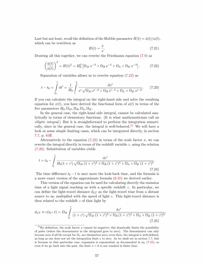
Last but not least, recall the definition of the Hubble parameterH(t) = a(t)/a(t),which can be rewritten as

H(t) =x

x. (7.21)

Drawing all this together, we can rewrite the Friedmann equation (7.9) as(a(t)

a(t)

)2

= H(t)2 = H20

[ΩM x−3 + ΩR x

−4 + ΩΛ + ΩK x−2]. (7.22)

Separation of variables allows us to rewrite equation (7.22) as

t− t0 =

t∫t0

dt′ =1

H0

x∫1

dx′

x′√

ΩM x′−3 + ΩR x′−4 + ΩΛ + ΩK x′−2. (7.23)

If you can calculate the integral on the right-hand side and solve the resultingequation for x(t), you have derived the functional form of a(t) in terms of thefive parameters H0,ΩM ,ΩR,ΩΛ,ΩK .

In the general case, the right-hand side integral, cannot be calculated ana-lytically in terms of elementary functions. (It is what mathematicians call anelliptic integral.) But it is straightforward to perform the integration numeri-cally, since in the general case, the integral is well-behaved.15 We will have alook at some simple limiting cases, which can be integrated directly, in section7.7, p. 65ff.

Alternatively to the equation (7.23) in terms of the scale factor x, we canrewrite the integral directly in terms of the redshift variable z, using the relation(7.20). Substitution of variables yields

t = t0 −z∫

0

dz′

H0(1 + z′)√

ΩM (1 + z′)3 + ΩR (1 + z′)4 + ΩΛ + ΩK (1 + z′)2.

(7.24)The time difference t0 − t is once more the look-back time, and the formula is

a more exact version of the approximate formula (6.35) we derived earlier.This version of the equation can be used for calculating directly the emission

time of a light signal reaching us with a specific redshift z. In particular, wecan define the light-travel distance dLT as the light-travel time from a distantsource to us, multiplied with the speed of light c. This light-travel distance isthen related to the redshift z of that light by

dLT ≡ c(t0−t) = DH

z∫0

dz′

(1 + z′)√

ΩM (1 + z′)3 + ΩR (1 + z′)4 + ΩΛ + ΩK (1 + z′)2,

(7.25)

15By definition, the scale factor x cannot be negative; this drastically limits the possibilityof poles (where the denominator in the integrand goes to zero). The denominator can onlybecome zero if all Ωs except for ΩΛ are themselves zero; even then, the integral is well-defined,as long as one does not set the integration limit x to zero. As we shall see in section 7.7, thisis because in that particular case, expansion is exponential, as documented in eq. (7.45), soeven if we go back into the past, the limit x = 0 is not reached in finite time.

57

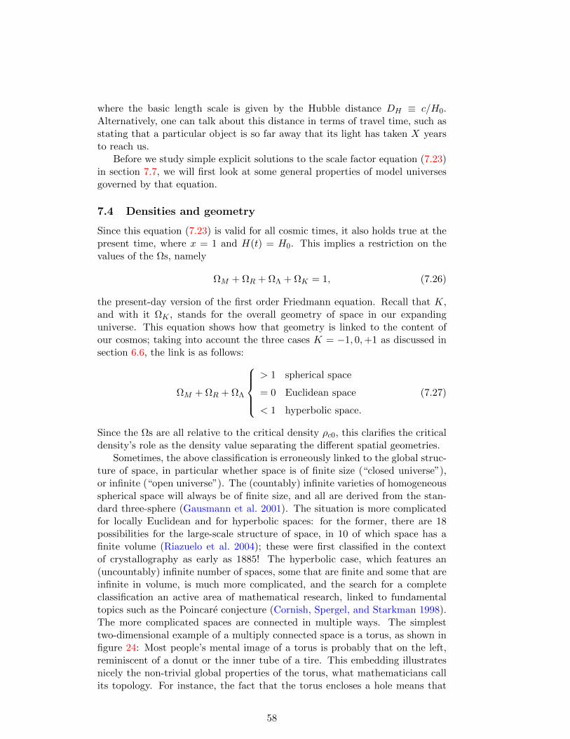
where the basic length scale is given by the Hubble distance DH ≡ c/H0.Alternatively, one can talk about this distance in terms of travel time, such asstating that a particular object is so far away that its light has taken X yearsto reach us.

Before we study simple explicit solutions to the scale factor equation (7.23)in section 7.7, we will first look at some general properties of model universesgoverned by that equation.

7.4 Densities and geometry

Since this equation (7.23) is valid for all cosmic times, it also holds true at thepresent time, where x = 1 and H(t) = H0. This implies a restriction on thevalues of the Ωs, namely

ΩM + ΩR + ΩΛ + ΩK = 1, (7.26)

the present-day version of the first order Friedmann equation. Recall that K,and with it ΩK , stands for the overall geometry of space in our expandinguniverse. This equation shows how that geometry is linked to the content ofour cosmos; taking into account the three cases K = −1, 0,+1 as discussed insection 6.6, the link is as follows:

ΩM + ΩR + ΩΛ

> 1 spherical space

= 0 Euclidean space

< 1 hyperbolic space.

(7.27)

Since the Ωs are all relative to the critical density ρc0, this clarifies the criticaldensity’s role as the density value separating the different spatial geometries.

Sometimes, the above classification is erroneously linked to the global struc-ture of space, in particular whether space is of finite size (“closed universe”),or infinite (“open universe”). The (countably) infinite varieties of homogeneousspherical space will always be of finite size, and all are derived from the stan-dard three-sphere (Gausmann et al. 2001). The situation is more complicatedfor locally Euclidean and for hyperbolic spaces: for the former, there are 18possibilities for the large-scale structure of space, in 10 of which space has afinite volume (Riazuelo et al. 2004); these were first classified in the contextof crystallography as early as 1885! The hyperbolic case, which features an(uncountably) infinite number of spaces, some that are finite and some that areinfinite in volume, is much more complicated, and the search for a completeclassification an active area of mathematical research, linked to fundamentaltopics such as the Poincare conjecture (Cornish, Spergel, and Starkman 1998).The more complicated spaces are connected in multiple ways. The simplesttwo-dimensional example of a multiply connected space is a torus, as shown infigure 24: Most people’s mental image of a torus is probably that on the left,reminiscent of a donut or the inner tube of a tire. This embedding illustratesnicely the non-trivial global properties of the torus, what mathematicians callits topology. For instance, the fact that the torus encloses a hole means that

58

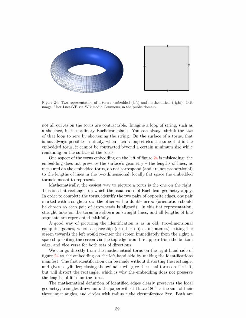
Figure 24: Two representation of a torus: embedded (left) and mathematical (right). Leftimage: User LucasVB via Wikimedia Commons, in the public domain.

not all curves on the torus are contractable. Imagine a loop of string, such asa shoelace, in the ordinary Euclidean plane. You can always shrink the sizeof that loop to zero by shortening the string. On the surface of a torus, thatis not always possible – notably, when such a loop circles the tube that is theembedded torus, it cannot be contracted beyond a certain minimum size whileremaining on the surface of the torus.

One aspect of the torus embedding on the left of figure 24 is misleading: theembedding does not preserve the surface’s geometry – the lengths of lines, asmeasured on the embedded torus, do not correspond (and are not proportional)to the lengths of lines in the two-dimensional, locally flat space the embeddedtorus is meant to represent.

Mathematically, the easiest way to picture a torus is the one on the right.This is a flat rectangle, on which the usual rules of Euclidean geometry apply.In order to complete the torus, identify the two pairs of opposite edges, one pairmarked with a single arrow, the other with a double arrow (orientation shouldbe chosen so each pair of arrowheads is aligned). In this flat representation,straight lines on the torus are shown as straight lines, and all lengths of linesegments are represented faithfully.

A good way of picturing the identification is as in old, two-dimensionalcomputer games, where a spaceship (or other object of interest) exiting thescreen towards the left would re-enter the screen immediately from the right; aspaceship exiting the screen via the top edge would re-appear from the bottomedge, and vice versa for both sets of directions.

We can go directly from the mathematical torus on the right-hand side offigure 24 to the embedding on the left-hand side by making the identificationsmanifest. The first identification can be made without distorting the rectangle,and gives a cylinder; closing the cylinder will give the usual torus on the left,but will distort the rectangle, which is why the embedding does not preservethe lengths of lines on the torus.

The mathematical definition of identified edges clearly preserves the localgeometry; triangles drawn onto the paper will still have 180 as the sum of theirthree inner angles, and circles with radius r the circumference 2πr. Both are

59

diagnostics that clearly show that this is locally Euclidean geometry. Similarly,the more complicated spaces belonging to expanding universes will locally havea spherical, or Euclidean, or hyperbolic geometry, but will be multiply con-nected.

7.5 Different eras of cosmic history; the Big Bang singularity

The general solution of the Friedmann equation (7.23) for the scale factor a(t)is not readily written down in terms of elementary functions — although easyenough to solve numerically. We can, however, make some fairly general state-ments about solutions.

The first batch of general statements follows directly from the scaling be-haviour of the different content types, which we had derived in section 6.1 fromthe equations of state. If a grows ever larger, then if dark energy is present,it will come eventually to dominate any further evolution, simply because theother densities have been diluted away, ρM ∼ a−3 and ρR ∼ a−4. If a wasvery small in the past, then if there is a radiation component, it will have beendominant back then because of ρR ∼ (1/a)4. In between, there may have beena phase where matter was the dominant contribution to the overall density, ata time when the density due to radiation had already been diluted, but beforedark energy becomes dominant.

This progression of various eras of dominance is fairly generic whenever allthree components are present; an example, using the best estimates for densityvalues in our own universe (cf. table 2 on page 67), is shown in figure 25.

10−6 10−5 10−4 10−3 10−2 10−1 100 101 10210−14

10−7

100

107

1014

1021

Relative scale factor a(t)/a(t0)

Den

sity

/pre

sent

den

sity

Radiation

Dark energy

Matter

Figure 25: Different types of content dominate at different scale factors: fairly generic pro-gression of eras, using the estimates for our own universe given in table 2 on page 67

In this diagram with two logarithmic scales, the line representing the matterdensity has slope −3, the radiation line −4, while dark energy density remains,

60

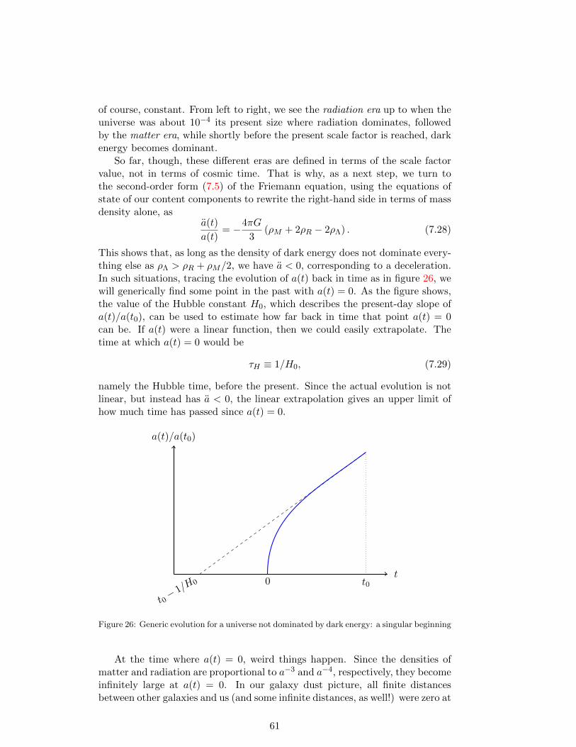
of course, constant. From left to right, we see the radiation era up to when theuniverse was about 10−4 its present size where radiation dominates, followedby the matter era, while shortly before the present scale factor is reached, darkenergy becomes dominant.

So far, though, these different eras are defined in terms of the scale factorvalue, not in terms of cosmic time. That is why, as a next step, we turn tothe second-order form (7.5) of the Friemann equation, using the equations ofstate of our content components to rewrite the right-hand side in terms of massdensity alone, as

a(t)

a(t)= −4πG

3(ρM + 2ρR − 2ρΛ) . (7.28)

This shows that, as long as the density of dark energy does not dominate every-thing else as ρΛ > ρR + ρM/2, we have a < 0, corresponding to a deceleration.In such situations, tracing the evolution of a(t) back in time as in figure 26, wewill generically find some point in the past with a(t) = 0. As the figure shows,the value of the Hubble constant H0, which describes the present-day slope ofa(t)/a(t0), can be used to estimate how far back in time that point a(t) = 0can be. If a(t) were a linear function, then we could easily extrapolate. Thetime at which a(t) = 0 would be

τH ≡ 1/H0, (7.29)

namely the Hubble time, before the present. Since the actual evolution is notlinear, but instead has a < 0, the linear extrapolation gives an upper limit ofhow much time has passed since a(t) = 0.

a(t)/a(t0)

t

t0− 1/

H0 t00

Figure 26: Generic evolution for a universe not dominated by dark energy: a singular beginning

At the time where a(t) = 0, weird things happen. Since the densities ofmatter and radiation are proportional to a−3 and a−4, respectively, they becomeinfinitely large at a(t) = 0. In our galaxy dust picture, all finite distancesbetween other galaxies and us (and some infinite distances, as well!) were zero at

61

that time. With these disquieting properties, the point at which a(t) = 0 is a so-called singularity, more specifically the initial singularity, Big Bang singularity,or just Big Bang for short. The time of that singularity is commonly chosen asthe zero point of cosmic time t = 0.

Our argument for why the Big Bang singularity must occur is a very crudeversion of much more rigorous singularity theorems, notably the cosmologicalsingularity theorem first formulated by Stephen Hawking and Roger Penrose,which show that Big Bang singularities occur under much more general circum-stances than in simple homogeneous models.

The Big Bang singularity is a problem for our models; in fact, singularitiesand infinities like this commonly indicate the limits of the model in question. Awidely accepted limit that would apply at such small scales in any case wouldbe that neither our simplified description nor the more complete description inthe framework of general relativity takes into account quantum effects, whichone should expect to become important at such small length scales and suchhigh energies. Unfortunately, no consistent and complete theory of quantumgravity has been found yet, although physicists have been searching for one forthe past 70+ years.

The good news is that, even without understanding the Big Bang singular-ity at t = 0, it is possible to model what happens directly afterwards, at a timewhen the universe was still very crowded, when the scale factor was smallerthan a thousandth of its present value, and densities for matter and radiationwere correspondingly high. The key factor in this is that, at present, the uni-verse contains about a billion times more photons than matter particles suchas protons, neutrons, and electrons. When we extrapolate back to smaller scalefactor values, when these photons were much more energetic (cosmic redshift!),we end up with a very hot soup of elementary particles, dominated by thesephotons — the Big Bang phase, sometimes called the Big Bang for short, aswell. The choice of terms here requires some caution: a cosmologist talkingabout the Big Bang could be referring to this [fairly well understood] phase ofthe early universe, or to the [highly problematic] Big Bang singularity — learnto deduce from the context what is meant!

The physics of the Big Bang phase is beyond the scope of this lecture, andwas covered at this summer school by Matthias Bartelmann’s lecture, a videorecording of which is available at

http://youtu.be/m35fXJoQLA0

The distinction between the Big Bang and the Big Bang phase is an im-portant one to make to both students and to the general public. Naturally,the Big Bang itself, as the beginning of everything, holds a special fascinationfor anyone interested in the big questions. It’s important to be honest at thispoint, and state clearly that cosmologists do not have reliable models for thatsingular beginning. We do not even know whether it is an abrupt beginning, ormerely the end of an earlier phase. But it is equally important to communicatethat this ignorance about the Big Bang singularity does not mean we can saynothing worthwhile about the beginning of the universe as we know it.

62

On the contrary: When it comes to the Big Bang phase, our knowledgebecomes more and more secure with increasing cosmic time, and after a bitless than a second of cosmic time, we have reached the realm of standard,experimentally testable physics. Our models of the Big Bang phase and itsaftermath have a lot to say about how the universe became what it is today– from the abundances of light elements to the existence and properties of thecosmic background radiation to the evolution the first stars, the first galaxies,and the large-scale structure of the observable universe.

Let us briefly talk about what a(0) = 0 does and doesn’t mean. Taken atface value, it does mean that all particles that are at finite distance from usat present had distance zero from us (and from each other) at the Big Bangsingularity at t = 0. In particular, everything we can observe around us, in otherwords: everything in the observable universe was, at that time zero, compressedinto an arbitrarily small volume. (The concept of the observable universe willbe made more precise in section 8.1.)

This does not necessarily mean that the whole universe was compressed intoa mathematical point. In those models where the universe is infinite, there areHubble flow galaxies that are infinitely far away from us at the present moment.Multiplying an infinite present distance with a zero-valued scale factor is an ill-defined problem. So is the Big Bang singularity a “spacetime point”, or in someway like a spacetime point, or not?

There is a way of understanding light propagation in relativistic spacetimesthat shows the situation to be more complicated. There exists a way of mappingeven an infinite universe into a finite, so-called conformal diagram (also knownas a Penrose diagram or, more rarely, Carter-Penrose diagram). Such mapsshow that when it comes to causality — which regions of spacetime can, inprinciple influence which other regions? — the initial singularity has morein common with infinite space than with an ordinary point in space (section5.3 in Hawking and Ellis 1973). For matter emerging from an ordinary singlepoint of space, one might assume that all this matter could have “inherited”common properties, such as a common temperature, from its common origin.But for matter shortly after the Big Bang, this kind of inheritance is impossible.Notably, a common origin of this particular kind is insufficient to explain thefact that early on, all baryonic matter in the observable universe appears to havehad nearly the same temperature (chapter 5 in Earman 1995). This is knownas the horizon problem, and one of the stated motivations of modifying theexpansion history of the very early universe by introducing an early inflationaryphase of exponential expansion prior to cosmic time t = 10−30 s.

Again, we will not go into the history of the very early universe in theselecture notes. We do take away the message that, in order to avoid confusion,if we feel the need to talk about how dense and compressed matter was in theearly universe, we had better avoid the singularity at t = 0. It is perfectlycorrect to say that, within these models, all the matter within the observableuniverse (alternatively, “all the matter we see around us”) was once compressedinto a volume the size of a basketball, or a cricket ball, or the pin of a needle,and so on. But talking about it all being compressed “into a single point”or “a region of volume zero” skips over significant complications, doesn’t add

63

anything significant in terms of understanding, and should not detract from thefacts that (a) within the general-relativistic models, the Big Bang singularity isnot part of spacetime, (b) the occurrence of the singularity a strong indicationthat our model breaks down at cosmic time t = 0, and (c) that at the presenttime, nobody has a solid alternative model for the very early universe.

On to less problematic matters: Now that we have chosen the zero point ofcosmic time t = 0 to correspond to the Big Bang singularity, at which x = 0,we can use equation (7.23) to obtain the age of the universe as

t0 =1

H0

1∫0

dx′

x′√

ΩM x′−3 + ΩR x′−4 + ΩΛ + ΩK x′−2. (7.30)

The time scale for the age of the universe is set by the Hubble time τH ≡ 1/H0

(cf. equation 7.29).

7.6 Expansion and collapse

Will an expanding universe keep expanding forever? Or might it collapse backonto itself, all pairwise distances now shrinking in proportion to the universalscale factor, just as they grew in unison before, ending in what has been calleda Big Crunch, as the opposite of the Big Bang (or, more facetiously, the GnabGib, [Adams 1980])?

For an answer, let us revisit the dimensionless Friedmann equation,(a(t)

a(t)

)2

= H(t)2 = H20

[ΩM x−3 + ΩR x

−4 + ΩΛ + ΩK x−2]. (7.22)

For an expansion phase a(t) > 0 to make the transition into a contractionphase with a(t) < 0, there must be a moment in between where a(t) = 0, andhence the whole equation (7.22) must be zero. Let us assume that if at all,this happens only after the early Big Bang phase, so that we can neglect theradiation term. Since x 6= 0, we can rewrite the condition that (7.22) be zeroas

ΩM + ΩΛx3 + ΩK x = 0, (7.31)

and since we know how to express ΩK in terms of the other two terms as perequation (7.26), the necessary condition for re-collapse is

ΩΛx3 + (1− ΩM − ΩΛ)x+ ΩM = 0. (7.32)

In the absence of any dark energy, ΩΛ = 0, this is readily solved as

x =ΩM

ΩM − 1, (7.33)

and since x must always be positive, this is only a solution if ΩM > 1, in otherwords: if the present-day matter density is larger than the present-day criticaldensity. In older text books, written before it was discovered that ΩΛ playeda significant role in our own universe, this circumstance was often linked to

64

space geometry: if only matter is present, a spherical geometry correspondsto a re-collapsing universe, while Euclidean and hyperbolic universes expandforever.

We can at least make some statements about the general case of equation(7.32). At the present day, x = 1, and we must have ΩM+ΩΛ+ΩK = 1 > 0. Andif ΩΛ < 0, corresponding to a type of dark energy that seeks to decelerate theuniverse, then for suitably large x, the cubic term will dominate, and the left-hand side of (7.32) will be negative; if it was positive before, and negative then,it must have been zero some time between. Will such large x values be reached,or could the evolution approach some constant x value, asymptotically? No,because then the acceleration would need to go to zero, which is not compatiblewith the acceleration equation (7.28). Such universes will always re-collapse.

For ΩΛ > 0, the situation is less clear, but it is clear that equation (7.32)can only be zero for some (necessarily positive!) x if the linear coefficient isnegative, 1− ΩM − ΩΛ = ΩK < 0. So in this case, as in the case without darkenergy, re-collapse is only possible if the space geometry is spherical. This is anecessary, but not a sufficient condition – for instance for ΩM = 0, there willbe no collapse even in a spherical space: in that case, the only solution for theturning point is

x =

√ΩΛ − 1

ΩΛ< 1, (7.34)

which, in a currently expanding universe, is a point in the past, when theuniverse was smaller. For there to be a turning point, we must have had auniverse that was initially collapsing, but then turned and is now expanding,and will keep expanding forever.

7.7 Explicit solutions

After these general considerations, let us turn to special cases of the Friedmannequation (7.23), which allow for simple solutions. We concentrate on solutionswith an initial singularity, and change the integration limits to include thesingularity a(0) = 0. Then we have

t =

t∫0

dt′ =

x∫0

dx′

H0x′√

ΩM x′−3 + ΩR x′−4 + ΩΛ + ΩK x′−2. (7.35)

We begin with a universe that contains only radiation — as we have seen insection 7.5, this is a good approximation for the very early universe, shortlyafter the Big Bang. Given the scaling of the term containing ΩK , we canneglect that term (and thus any non-Euclidean geometry of the universe) whenwe restrict ourselves to the early universe with small values of a. This leavesus with

t =

x∫0

dx′ x′

H0

√ΩR

=1

2H0

√ΩR

x2, (7.36)

which is readily solved as

a(t) = a(t0) ·√√

ΩR · 2H0t ∼ t1/2. (7.37)

65

If this is not just an approximation, with ΩK neglected, but instead a genericEuclidean model universe with ΩK = 0, then by the present-day Friedmannequation (7.26), which states that all the Ωs must sum up to one, we must haveΩR = 1, and our evolution is given by

a(t) = a(t0) ·√

2H0t. (7.38)

For consistency, if we insert the present age t0 of the universe, we must recovera(t = t0) = a(t0). This means that the age of a pure radiation universe mustbe given by

t0 =1

2H0, (7.39)

half the Hubble time, in other words: half as old as for a linearly expandinguniverse. In particular, this means that we can write the scale factor in theparticularly simple form

a(t) = a(t0) ·√t/t0. (7.40)

Next, consider a Euclidean (ΩK = 0), matter-only universe. This solution,which is called the Einstein–de-Sitter (EdS) universe, must have ΩM = 1 inorder to satisfy the present-day Friedmann equation (7.26). Integrating up, weobtain

a(t) = a(t0) · (3/2 ·H0t)2/3 ∼ t2/3. (7.41)

Again, consistency demands, and direct calculation of H(t) confirms, that theage t0 of such a universe must be

t0 =2

3H0, (7.42)

and the simplest form for the scale factor is

a(t) = a(t0) · (t/t0)2/3. (7.43)

Our last elementary case is a universe with Euclidean space (ΩK = 0) thatonly contains dark energy, so ΩΛ = 1. In this case, there will be no finite timeat which a(t) = 0, so we revert to the original integration limits of (7.23) toobtain

t− t0 =

x∫1

dx′

H0 x′=

1

H0ln(x) (7.44)

so thata(t) = a(t0) · exp [H0(t− t0)] . (7.45)

This type of exponential solution, albeit disguised by another choice of coor-dinates, was first found by the Dutch astronomer Willem de Sitter (de Sitter1917). In modern cosmology, it is important for the latest stages of evolution,when dark energy dominates, but also for a very early, hypothetical stage knownas inflation, postulated to explain, among other things, the homogeneity of theuniverse as well as the absence of certain exotic particles.

66

The de Sitter scale factor can also be written in terms of the cosmologicalconstant. In the de Sitter universe, the critical density (7.11) is equal to the darkenergy density, which can be expressed in terms of the cosmological constantas in equation (6.9). Equating the two, we have

H0 = c√

Λ/3, (7.46)

and can re-write the de Sitter scale factor as

a(t) = a(t0) · exp[√

Λ/3 · c (t− t0)]. (7.47)

This concludes our gallery of selected explicit solutions; a more complete overviewcan be found in chapter 23 of d’Inverno 1992 or chapter 9 of Rindler 1977.

With the arguments concerning the different eras, and these simple solu-tions, we can make a reasonable estimate for how a(t) looks for our own uni-verse. Our cosmos contains radiation (in particular the cosmic backgroundradiation), matter in the form of galaxies, and dark energy. Thus, we wouldexpect a beginning that looks like a(t) ∼ t1/2 while radiation dominates, ex-ponential expansion at the later stages, and some kind of interpolation linkingthe two.

Table 2: Parameter estimates for our universe

H0 = 67.74 km/s/Mpc= 1/(4.6 · 1017 s) = 1/(1.4 · 1010 a)

ΩΛ = 0.69

ΩM = 0.31

ΩR = 0.0001

The parameter values applying to our specific universe need to derive fromobservation. A set of realistic estimates combining the measurements of ESA’sPlanck satellite with other observations (notably of the redshift-distance re-lation, cf. section 8.4) can be found in table 2 (Planck Collaboration 2016).16

The matter part ΩM can be split in baryonic matter (such as protons, neutrons,electrons and the nuclei, atoms and molecules they form) with Ωb = 0.05 anda dark matter part with Ωdm = 0.26.

The critical density (7.11) in such a universe amounts to

ρc0 = 8.6 · 10−27 kg

m3= 4.8

GeV/c2

m3, (7.48)

which corresponds to about five proton masses per cubic meter.A numerical solution using these parameter values is shown in figure 27. The

16Rightmost column in table 4. The density parameter for radiation can be derived fromΩM and the redshift zeq specified in the table, which indicates the redshift at which matter andradiation density were equal. Given the scaling behaviour for radiation and matter discussedin section 6.1, we must have ΩR = ΩM/(1 + zeq), which yields the value for ΩR quoted intable 2.

67

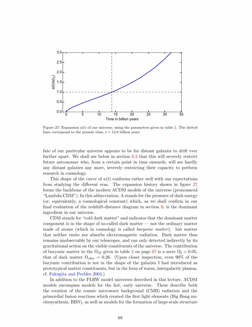
0 5 10 15 20 25 30 35Time in billion years

0.0

0.5

1.0

1.5

2.0

2.5

3.0a(

t)/a(

t 0)

Figure 27: Expansion a(t) of our universe, using the parameters given in table 2. The dottedlines correspond to the present time, t = 13.8 billion years

fate of our particular universe appears to be for distant galaxies to drift everfurther apart. We shall see below in section 8.3 that this will severely restrictfuture astronomer who, from a certain point in time onwards, will see hardlyany distant galaxies any more, severely restricting their capacity to performresearch in cosmology.

This shape of the curve of a(t) conforms rather well with our expectationsfrom studying the different eras. The expansion history shown in figure 27forms the backbone of the modern ΛCDM models of the universe (pronounced“Lambda-CDM”). In this abbreviation, Λ stands for the presence of dark energy(or, equivalently, a cosmological constant) which, as we shall confirm in ourfinal evaluation of the redshift-distance diagram in section 9, is the dominantingredient in our universe.

CDM stands for “cold dark matter” and indicates that the dominant mattercomponent is in the shape of so-called dark matter — not the ordinary mattermade of atoms (which in cosmology is called baryonic matter), but matterthat neither emits nor absorbs electromagnetic radiation. Dark matter thusremains unobservable by our telescopes, and can only detected indirectly by itsgravitational action on the visible constituents of the universe. The contributionof baryonic matter to the ΩM given in table 2 on page 67 is a mere Ωb = 0.05,that of dark matter Ωcdm = 0.26. (Upon closer inspection, even 90% of thebaryonic contribution is not in the shape of the galaxies I had introduced asprototypical matter constituents, but in the form of warm, intergalactic plasma,cf. Fukugita and Peebles 2004.)

In addition to the FLRW model universes described in this lecture, ΛCDMmodels encompass models for the hot, early universe. These describe boththe creation of the cosmic microwave background (CMB) radiation and theprimordial fusion reactions which created the first light elements (Big Bang nu-cleosynthesis, BBN), as well as models for the formation of large-scale structure

68

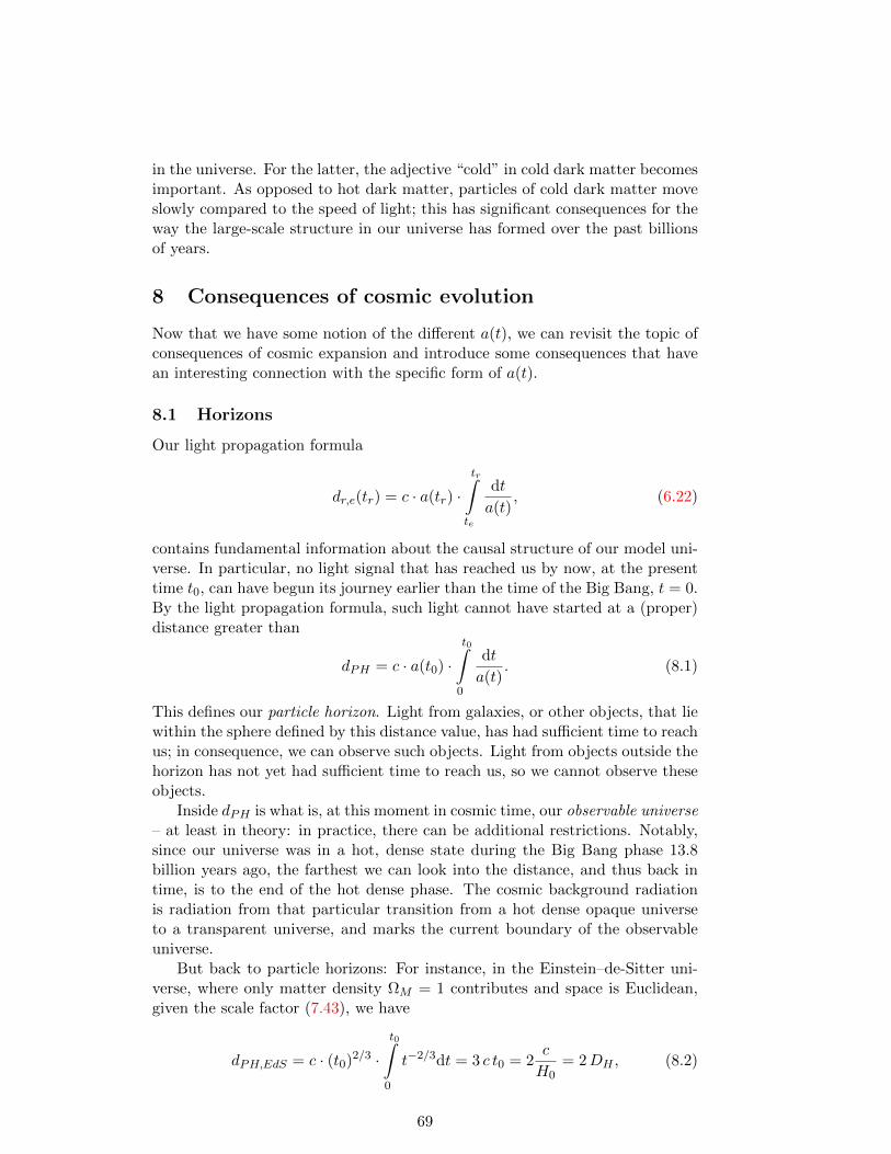
in the universe. For the latter, the adjective “cold” in cold dark matter becomesimportant. As opposed to hot dark matter, particles of cold dark matter moveslowly compared to the speed of light; this has significant consequences for theway the large-scale structure in our universe has formed over the past billionsof years.

8 Consequences of cosmic evolution

Now that we have some notion of the different a(t), we can revisit the topic ofconsequences of cosmic expansion and introduce some consequences that havean interesting connection with the specific form of a(t).

8.1 Horizons

Our light propagation formula

dr,e(tr) = c · a(tr) ·tr∫te

dt

a(t), (6.22)

contains fundamental information about the causal structure of our model uni-verse. In particular, no light signal that has reached us by now, at the presenttime t0, can have begun its journey earlier than the time of the Big Bang, t = 0.By the light propagation formula, such light cannot have started at a (proper)distance greater than

dPH = c · a(t0) ·t0∫

0

dt

a(t). (8.1)

This defines our particle horizon. Light from galaxies, or other objects, that liewithin the sphere defined by this distance value, has had sufficient time to reachus; in consequence, we can observe such objects. Light from objects outside thehorizon has not yet had sufficient time to reach us, so we cannot observe theseobjects.

Inside dPH is what is, at this moment in cosmic time, our observable universe– at least in theory: in practice, there can be additional restrictions. Notably,since our universe was in a hot, dense state during the Big Bang phase 13.8billion years ago, the farthest we can look into the distance, and thus back intime, is to the end of the hot dense phase. The cosmic background radiationis radiation from that particular transition from a hot dense opaque universeto a transparent universe, and marks the current boundary of the observableuniverse.

But back to particle horizons: For instance, in the Einstein–de-Sitter uni-verse, where only matter density ΩM = 1 contributes and space is Euclidean,given the scale factor (7.43), we have

dPH,EdS = c · (t0)2/3 ·t0∫

0

t−2/3dt = 3 c t0 = 2c

H0= 2DH , (8.2)

69

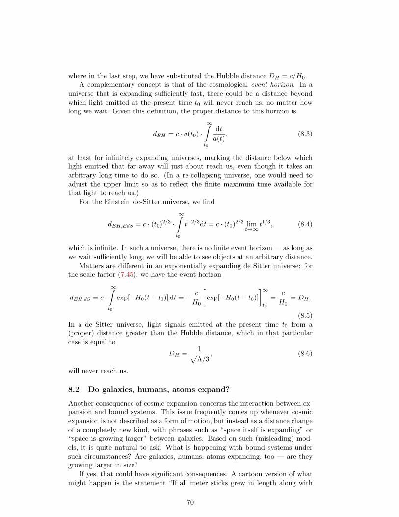
where in the last step, we have substituted the Hubble distance DH = c/H0.A complementary concept is that of the cosmological event horizon. In a

universe that is expanding sufficiently fast, there could be a distance beyondwhich light emitted at the present time t0 will never reach us, no matter howlong we wait. Given this definition, the proper distance to this horizon is

dEH = c · a(t0) ·∞∫t0

dt

a(t), (8.3)

at least for infinitely expanding universes, marking the distance below whichlight emitted that far away will just about reach us, even though it takes anarbitrary long time to do so. (In a re-collapsing universe, one would need toadjust the upper limit so as to reflect the finite maximum time available forthat light to reach us.)

For the Einstein–de-Sitter universe, we find

dEH,EdS = c · (t0)2/3 ·∞∫t0

t−2/3dt = c · (t0)2/3 limt→∞

t1/3, (8.4)

which is infinite. In such a universe, there is no finite event horizon — as long aswe wait sufficiently long, we will be able to see objects at an arbitrary distance.

Matters are different in an exponentially expanding de Sitter universe: forthe scale factor (7.45), we have the event horizon

dEH,dS = c ·∞∫t0

exp[−H0(t− t0)] dt = − c

H0

[exp[−H0(t− t0)]

]∞t0

=c

H0= DH .

(8.5)In a de Sitter universe, light signals emitted at the present time t0 from a(proper) distance greater than the Hubble distance, which in that particularcase is equal to

DH =1√Λ/3

, (8.6)

will never reach us.

8.2 Do galaxies, humans, atoms expand?

Another consequence of cosmic expansion concerns the interaction between ex-pansion and bound systems. This issue frequently comes up whenever cosmicexpansion is not described as a form of motion, but instead as a distance changeof a completely new kind, with phrases such as “space itself is expanding” or“space is growing larger” between galaxies. Based on such (misleading) mod-els, it is quite natural to ask: What is happening with bound systems undersuch circumstances? Are galaxies, humans, atoms expanding, too — are theygrowing larger in size?

If yes, that could have significant consequences. A cartoon version of whatmight happen is the statement “If all meter sticks grew in length along with

70

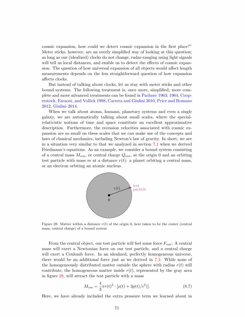
cosmic expansion, how could we detect cosmic expansion in the first place?”Meter sticks, however, are an overly simplified way of looking at this question;as long as our (idealized) clocks do not change, radar-ranging using light signalswill tell us local distances, and enable us to detect the effects of cosmic expan-sion. The question of how universal expansion of all objects would affect lengthmeasurements depends on the less straightforward question of how expansionaffects clocks.

But instead of talking about clocks, let us stay with meter sticks and otherbound systems. The following treatment is, once more, simplified; more com-plete and more advanced treatments can be found in Pachner 1963; 1964, Coop-erstock, Faraoni, and Vollick 1998, Carrera and Giulini 2010, Price and Romano2012, Giulini 2014.

When we talk about atoms, humans, planetary systems and even a singlegalaxy, we are automatically talking about small scales, where the special-relativistic notions of time and space constitute an excellent approximativedescription. Furthermore, the recession velocities associated with cosmic ex-pansion are so small on these scales that we can make use of the concepts andlaws of classical mechanics, including Newton’s law of gravity. In short, we arein a situation very similar to that we analyzed in section 7.1 when we derivedFriedmann’s equations. As an example, we consider a bound system consistingof a central mass Mcen, or central charge Qcen, at the origin 0 and an orbitingtest particle with mass m at a distance r(t): a planet orbiting a central mass,or an electron orbiting an atomic nucleus.

testparticle

0

r(t)

Figure 28: Matter within a distance r(t) of the origin 0, here taken to be the center (centralmass, central charge) of a bound system

From the central object, our test particle will feel some force Fcen: A centralmass will exert a Newtonian force on our test particle, and a central chargewill exert a Coulomb force. In an idealized, perfectly homogeneous universe,there would be an additional force just as we derived in 7.1: While none ofthe homogeneously distributed matter outside the sphere with radius r(t) willcontribute, the homogeneous matter inside r(t), represented by the gray areain figure 28, will attract the test particle with a mass

Mcos =4

3πr(t)3 · [ρ(t) + 3p(t)/c2)]. (8.7)

Here, we have already included the extra pressure term we learned about in

71

section 3.5, and where the density ρ includes contributions from the energydensity. For short, we will refer to the mass of the homogeneous matter, andto the force on the test particle resulting from it, as “cosmological”, Mcos andFcos respectively, in order to distinguish it from the central force Fcen.

That mass Mcos will act as if it were the mass of a point particle at theorigin, so the gravitational force from the homogeneous matter that our testparticle feels will be radial, and of the strength

Fcos = −4G

3πr(t) ·m[ρ(t) + 3p(t)/c2]. (8.8)

Which kinds of cosmic matter contribute to this force Fcos? Ordinary matter,while assumed to be homogeneous on large scales, is most certainly not homo-geneously distributed on the scales of atoms, humans, or planetary systems.When we talk about atoms and their typical length scales, all of the ordinarymatter except for the atomic nucleus, whose influence is accounted for in Fcen,will be outside, and not contribute to Fcos.

Does dark matter contribute? If dark matter is in the form of particles, asis commonly believed, that would depend on the particle mass. Going by theparameter estimate based listed in table 2 on page 67 and the critical densityvalue in (7.48), the present mass density of dark matter amounts to

ρdm = Ωdm ρc0 = 2.2 · 10−27 kg

m3= 1.2

GeV/c2

m3. (8.9)

No dark matter particle has yet been detected, and estimates for their massesdepend on the chosen hypothetical model. For so-called axions, their (current)masses could be in the range of 0.1 meV/c2, corresponding to ∼ 1013 suchparticles per cubic meter. But the typical volume of an atom is on the orderof 10−29 m3 at most. The probability to find a single one of these dark matterparticles inside a randomly placed atom would be 10−16. One might try tocalculate the minute influence these particles might have on an atom whenthey happen to pass through, but numbers are such that approximating darkmatter as a homogeneous continuum on the scale of atoms makes no sense. Thenumbers are, of course, much worse, for heavier dark matter candidates, suchas WIMPs (for “weakly interacting massive particle”) with expected massesof 10 GeV/c2 and more (Patrignani and Particle Data Group 2016). On theother hand, over planet- or solar-system-size volumes, we will find so manyeven of these heavy particles that a homogeneous distribution should be a goodapproximation.

Inserting the respective equations of state (6.8) for dark matter and darkenergy into equation (8.8) and, in a second step, the definition of the criticaldensity (7.11), we find that

Fcos =4πG

3rm[2ρΛ − ρdm] = mrH2

0 [ΩΛ − Ωdm/2]. (8.10)

On atomic or molecular scales, as per the argument given above, we will neglectthe dark matter contribution; on planetary scales and above we will include dark

72

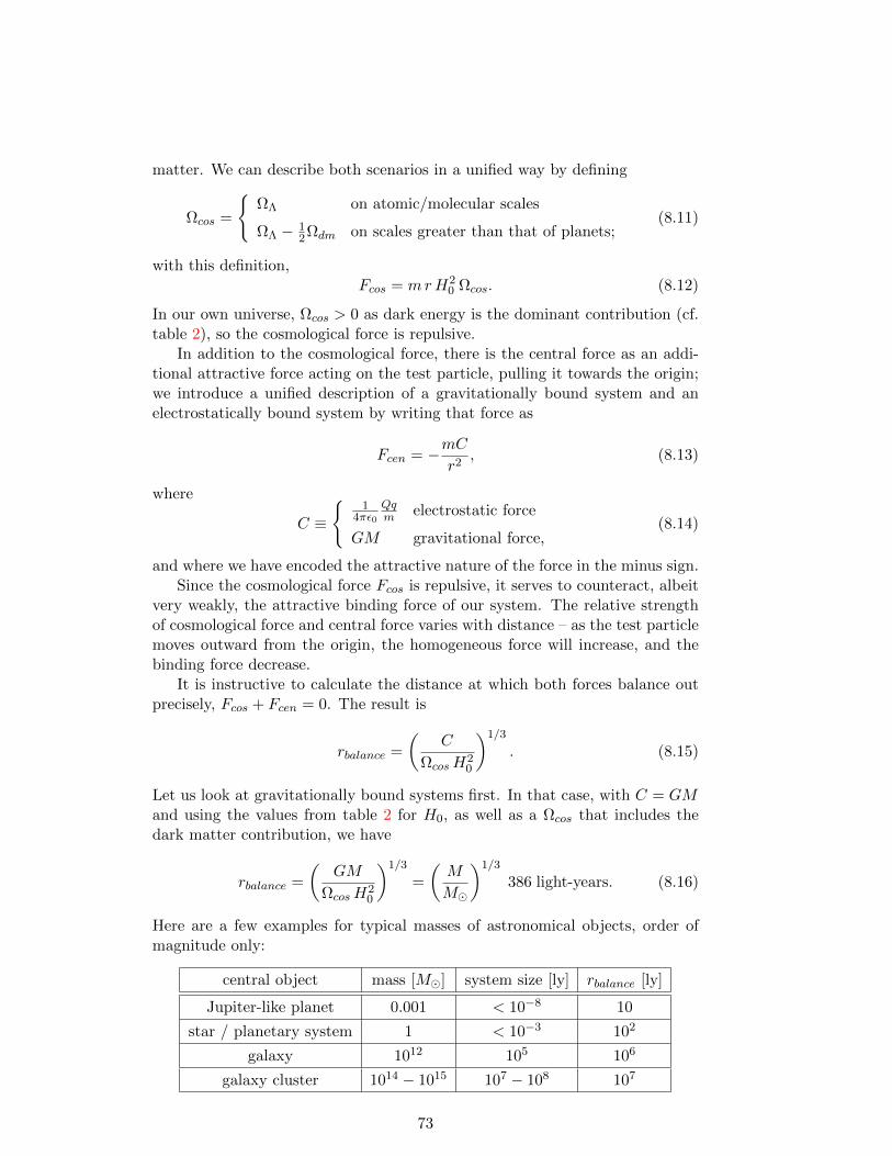
matter. We can describe both scenarios in a unified way by defining

Ωcos =

ΩΛ on atomic/molecular scales

ΩΛ − 12Ωdm on scales greater than that of planets;

(8.11)

with this definition,Fcos = mrH2

0 Ωcos. (8.12)

In our own universe, Ωcos > 0 as dark energy is the dominant contribution (cf.table 2), so the cosmological force is repulsive.

In addition to the cosmological force, there is the central force as an addi-tional attractive force acting on the test particle, pulling it towards the origin;we introduce a unified description of a gravitationally bound system and anelectrostatically bound system by writing that force as

Fcen = −mCr2

, (8.13)

where

C ≡

1

4πε0Qqm electrostatic force

GM gravitational force,(8.14)

and where we have encoded the attractive nature of the force in the minus sign.Since the cosmological force Fcos is repulsive, it serves to counteract, albeit

very weakly, the attractive binding force of our system. The relative strengthof cosmological force and central force varies with distance – as the test particlemoves outward from the origin, the homogeneous force will increase, and thebinding force decrease.

It is instructive to calculate the distance at which both forces balance outprecisely, Fcos + Fcen = 0. The result is

rbalance =

(C

ΩcosH20

)1/3

. (8.15)

Let us look at gravitationally bound systems first. In that case, with C = GMand using the values from table 2 for H0, as well as a Ωcos that includes thedark matter contribution, we have

rbalance =

(GM

ΩcosH20

)1/3

=

(M

M

)1/3

386 light-years. (8.16)

Here are a few examples for typical masses of astronomical objects, order ofmagnitude only:

central object mass [M] system size [ly] rbalance [ly]

Jupiter-like planet 0.001 < 10−8 10

star / planetary system 1 < 10−3 102

galaxy 1012 105 106

galaxy cluster 1014 − 1015 107 − 108 107

73

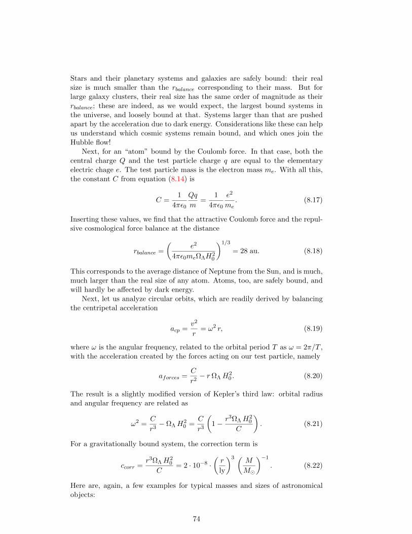
Stars and their planetary systems and galaxies are safely bound: their realsize is much smaller than the rbalance corresponding to their mass. But forlarge galaxy clusters, their real size has the same order of magnitude as theirrbalance; these are indeed, as we would expect, the largest bound systems inthe universe, and loosely bound at that. Systems larger than that are pushedapart by the acceleration due to dark energy. Considerations like these can helpus understand which cosmic systems remain bound, and which ones join theHubble flow!

Next, for an “atom” bound by the Coulomb force. In that case, both thecentral charge Q and the test particle charge q are equal to the elementaryelectric chage e. The test particle mass is the electron mass me. With all this,the constant C from equation (8.14) is

C =1

4πε0

Qq

m=

1

4πε0

e2

me. (8.17)

Inserting these values, we find that the attractive Coulomb force and the repul-sive cosmological force balance at the distance

rbalance =

(e2

4πε0meΩΛH20

)1/3

= 28 au. (8.18)

This corresponds to the average distance of Neptune from the Sun, and is much,much larger than the real size of any atom. Atoms, too, are safely bound, andwill hardly be affected by dark energy.

Next, let us analyze circular orbits, which are readily derived by balancingthe centripetal acceleration

acp =v2

r= ω2 r, (8.19)

where ω is the angular frequency, related to the orbital period T as ω = 2π/T ,with the acceleration created by the forces acting on our test particle, namely

aforces =C

r2− rΩΛH

20 . (8.20)

The result is a slightly modified version of Kepler’s third law: orbital radiusand angular frequency are related as

ω2 =C

r3− ΩΛH

20 =

C

r3

(1− r3ΩΛH

20

C

). (8.21)

For a gravitationally bound system, the correction term is

ccorr =r3ΩΛH

20

C= 2 · 10−8 ·

(r

ly

)3 ( M

M

)−1

. (8.22)

Here are, again, a few examples for typical masses and sizes of astronomicalobjects:

74

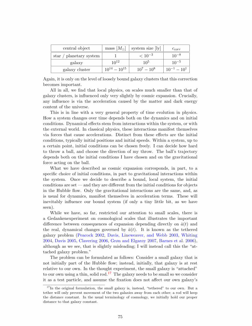
central object mass [M] system size [ly] ccorr

star / planetary system 1 < 10−3 10−8

galaxy 1012 105 10−5

galaxy cluster 1014 − 1015 107 − 108 10−1 − 101

Again, it is only on the level of loosely bound galaxy clusters that this correctionbecomes important.

All in all, we find that local physics, on scales much smaller than that ofgalaxy clusters, is influenced only very slightly by cosmic expansion. Crucially,any influence is via the acceleration caused by the matter and dark energycontent of the universe.

This is in line with a very general property of time evolution in physics.How a system changes over time depends both on the dynamics and on initialconditions. Dynamical effects stem from interactions within the system, or withthe external world. In classical physics, these interactions manifest themselvesvia forces that cause accelerations. Distinct from these effects are the initialconditions, typically initial positions and initial speeds. Within a system, up toa certain point, initial conditions can be chosen freely. I can decide how hardto throw a ball, and choose the direction of my throw. The ball’s trajectorydepends both on the initial conditions I have chosen and on the gravitationalforce acting on the ball.

What we have described as cosmic expansion corresponds, in part, to aspecific choice of initial conditions, in part to gravitational interactions withinthe system. Once we decide to describe a bound, local system, the initialconditions are set — and they are different from the initial conditions for objectsin the Hubble flow. Only the gravitational interactions are the same, and, asis usual for dynamics, manifest themselves in acceleration terms. These willinevitably influence our bound system (if only a tiny little bit, as we haveseen).

While we have, so far, restricted our attention to small scales, there isa Gedankenexperiment on cosmological scales that illustrates the importantdifference between consequences of expansion depending directly on a(t) andthe real, dynamical changes governed by a(t). It is known as the tetheredgalaxy problem (Peacock 2002, Davis, Lineweaver, and Webb 2003, Whiting2004, Davis 2005, Clavering 2006, Grøn and Elgarøy 2007, Barnes et al. 2006),although as we see, that is slightly misleading; I will instead call this the “at-tached galaxy problem.”

The problem can be formulated as follows: Consider a small galaxy that isnot initially part of the Hubble flow; instead, initially, that galaxy is at restrelative to our own. In the thought experiment, the small galaxy is “attached”to our own using a thin, solid rod.17 The galaxy needs to be small so we considerit as a test particle, and assume the fixation does not affect our own galaxy’s

17In the original formulation, the small galaxy is, instead, “tethered” to our own. But atether will only prevent movement of the two galaxies away from each other; a rod will keepthe distance constant. In the usual terminology of cosmology, we initially hold our properdistance to that galaxy constant.

75

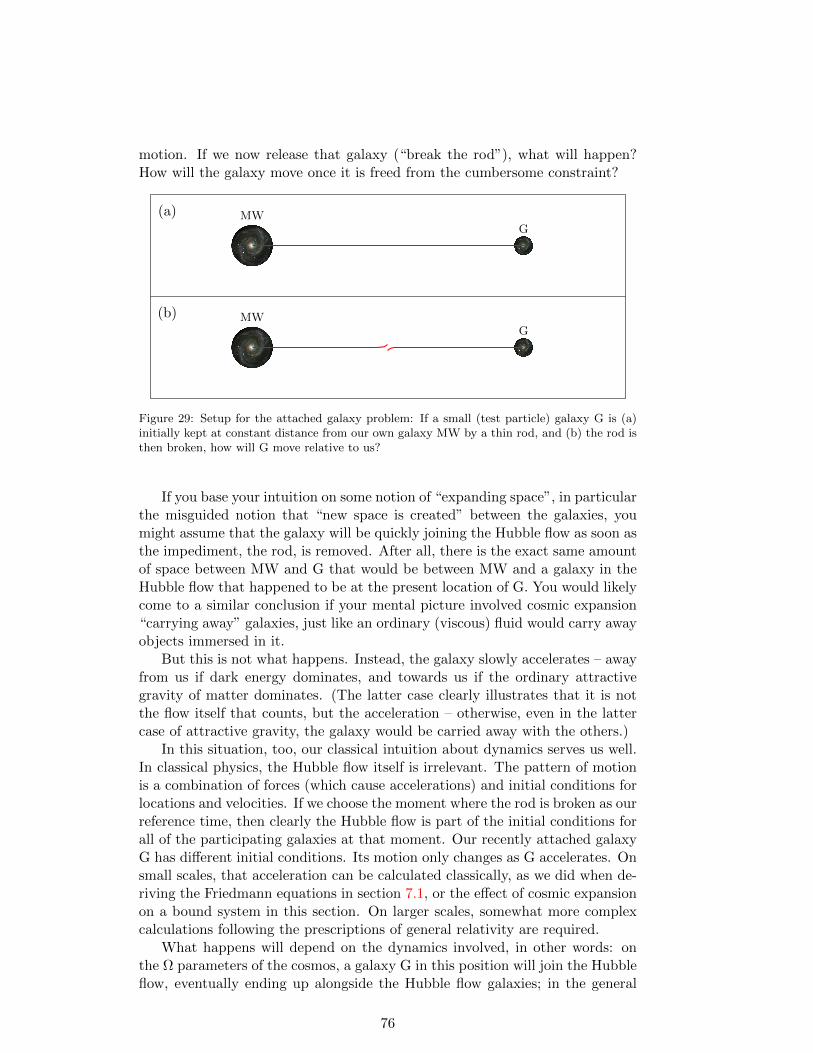
motion. If we now release that galaxy (“break the rod”), what will happen?How will the galaxy move once it is freed from the cumbersome constraint?

MWG

(b)

(a) MWG

Figure 29: Setup for the attached galaxy problem: If a small (test particle) galaxy G is (a)initially kept at constant distance from our own galaxy MW by a thin rod, and (b) the rod isthen broken, how will G move relative to us?

If you base your intuition on some notion of “expanding space”, in particularthe misguided notion that “new space is created” between the galaxies, youmight assume that the galaxy will be quickly joining the Hubble flow as soon asthe impediment, the rod, is removed. After all, there is the exact same amountof space between MW and G that would be between MW and a galaxy in theHubble flow that happened to be at the present location of G. You would likelycome to a similar conclusion if your mental picture involved cosmic expansion“carrying away” galaxies, just like an ordinary (viscous) fluid would carry awayobjects immersed in it.

But this is not what happens. Instead, the galaxy slowly accelerates – awayfrom us if dark energy dominates, and towards us if the ordinary attractivegravity of matter dominates. (The latter case clearly illustrates that it is notthe flow itself that counts, but the acceleration – otherwise, even in the lattercase of attractive gravity, the galaxy would be carried away with the others.)

In this situation, too, our classical intuition about dynamics serves us well.In classical physics, the Hubble flow itself is irrelevant. The pattern of motionis a combination of forces (which cause accelerations) and initial conditions forlocations and velocities. If we choose the moment where the rod is broken as ourreference time, then clearly the Hubble flow is part of the initial conditions forall of the participating galaxies at that moment. Our recently attached galaxyG has different initial conditions. Its motion only changes as G accelerates. Onsmall scales, that acceleration can be calculated classically, as we did when de-riving the Friedmann equations in section 7.1, or the effect of cosmic expansionon a bound system in this section. On larger scales, somewhat more complexcalculations following the prescriptions of general relativity are required.

What happens will depend on the dynamics involved, in other words: onthe Ω parameters of the cosmos, a galaxy G in this position will join the Hubbleflow, eventually ending up alongside the Hubble flow galaxies; in the general

76

case, however, a galaxy G in such a situation will not join the Hubble flow.18

Returning to bound system one last time, it should be noted that there are(speculative) hypothetical scenarios that lead to much more dramatic conse-quences for bound systems in the future (Caldwell, Kamionkowski, and Wein-berg 2003). As we saw in section 6.1, the dilution behaviour of different kindsof matter content (including dark energy) depends crucially on the equation ofstate. In all cases of interest to standard cosmology, that equation has the form(6.8),

p = w · ρc2, (6.8)

and we have seen in equation (6.13) that depending on the value of w, thecorresponding density will change as

ρ(t) = ρ(t0) ·(a(t)

a(t0)

)−3(1+w)

. (6.13)

On the other hand, both in the second-order Friedmann equation (7.5) and inthe corresponding equation (8.8) for the additional force acting within a boundsystem due to homogeneous cosmological terms, the gravitational attraction isproportional to

ρ+ 3p/c2. (8.23)

Under these circumstances, an ingredient with w < −1 would have a dramaticeffect. By (8.23), such an ingredient, which has been dubbed phantom energy,would exert a repulsive force on bound systems, similar to the influence of darkenergy we have already explored in this section. But unlike dark energy, thedensity of this hypothetical ingredient would not remain constant, but growlarger with cosmic expansion, as per equation (6.13). In consequence, the radiirbalance where the repulsive force and a bound system’s attractive force balancewould grow ever smaller, and one after the other, bound systems on ever smallerscales would be ripped apart: galaxy clusters, galaxies, stars, planets, humans,atoms, atomic nuclei. Within a finite time, it turns out, the repulsive influencewould become infinitely strong. The universe would end in a Big Rip. Atpresent, however, there is no evidence whatsoever that such phantom energyexists in our cosmos.

8.3 The fate of our own universe

Given that our own universe is currently dominated by dark energy, and willcontinue to be so dominated, expansion is set to continue indefinitely – bar-ring effects so unusual that they are not included in the current cosmologicalstandard models. By that token, the event horizon for the de Sitter universeis relevant for our distant future, making for a lonely long-term fate. We canexplore the specifics as follows (in a way similar to that of the article of Kraussand Starkman 2000):

As a first step, let us extrapolate into the future, to the time t100 when thescale factor will be 100 times larger than it is today. We can calculate that time

18The details depend on your definition of joining the Hubble flow, cf. Barnes et al. 2006.

77

using equation (7.35), namely as

t100 =1

H0

100∫0

dx′

x′√

ΩMx′−3 + ΩΛ

. (8.24)

Using the values given in table 2 on page 67, this can be evaluated numericallyas

t100 =6.4

H0= 9 · 1011 a. (8.25)

At that time, by the dimensionless Friedmann equation (7.22), the Hubbleconstant will be

H100 ≈ H0 ·√

ΩΛ, (8.26)

the matter term ΩM being suppressed by a factor 10−6. By the same reason-ing, scale factor evolution will be described in very good approximation by anexponentially expanding universe, equation (7.45), namely

a(t) = a100 · exp[H100(t− t100)] = 100 · a0 · exp[H0

√ΩΛ(t− t100)]. (8.27)

On this basis, we can look at the cosmic event horizon. In equation (8.3), wehad written down the event horizon at the present time t0. At any later timet, the event horizon, as a proper distance measured at that future time t, is

dEH(t) = c · a(t) ·∞∫t

dt′

a(t′). (8.28)

But what we are really interested in is the proper distance as measured todaythat value corresponds to. That will tell us which of the objects in the present-day universe we will be able to see in the future, and which not. Since properdistances are directly proportional to the scale factor, the conversion is simple– a factor a(t0)/a(t) will do the trick, so

dEH,0(t) =a0

a(t)dEH(t) = c · a0 ·

∞∫t

dt′

a(t′), (8.29)

which is the event horizon at time t, expressed as a present-day proper distance.Restricting ourselves to t > t100 and using (8.27) to describe cosmic evolutionduring that epoch, we find

dEH,0(t) =c

100H0

√ΩΛ

exp[−H0

√ΩΛ(t− t100)

]. (8.30)

As time passes, the event horizon shrinks further and further, separating usfrom ever closer regions in the present-day universe. Figure 30 shows a plot ofdEH,0(t) against cosmic time. This plot should be read as follows: Pick somefuture time t on the x axis, say: a cosmic time of 100 billion years (as shownby the dotted lines). The value of the curve shows you that those galaxies inthe Hubble flow that currently, at the present time, have a proper distance

78

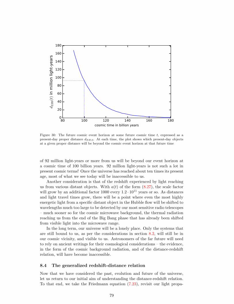
80 100 120 140 160 180

cosmic time in billion years

0

20

40

60

80

100

120

140

160

180

dEH

0(t

) in

mill

ion lig

ht-

years

Figure 30: The future cosmic event horizon at some future cosmic time t, expressed as apresent-day proper distance dEH,0. At each time, the plot shows which present-day objectsat a given proper distance will be beyond the cosmic event horizon at that future time

of 92 million light-years or more from us will be beyond our event horizon ata cosmic time of 100 billion years. 92 million light-years is not such a lot inpresent cosmic terms! Once the universe has reached about ten times its presentage, most of what we see today will be inaccessible to us.

Another consideration is that of the redshift experienced by light reachingus from various distant objects. With a(t) of the form (8.27), the scale factorwill grow by an additional factor 1000 every 1.2 · 1011 years or so. As distancesand light travel times grow, there will be a point where even the most highlyenergetic light from a specific distant object in the Hubble flow will be shifted towavelengths much too large to be detected by our most sensitive radio telescopes– much sooner so for the cosmic microwave background, the thermal radiationreaching us from the end of the Big Bang phase that has already been shiftedfrom visible light into the microwave range.

In the long term, our universe will be a lonely place. Only the systems thatare still bound to us, as per the considerations in section 8.2, will still be inour cosmic vicinity, and visible to us. Astronomers of the far future will needto rely on ancient writings for their cosmological considerations – the evidence,in the form of the cosmic background radiation, and of the distance-redshiftrelation, will have become inaccessible.

8.4 The generalized redshift-distance relation

Now that we have considered the past, evolution and future of the universe,let us return to our initial aim of understanding the distance-redshift relation.To that end, we take the Friedmann equation (7.23), revisit our light propa-

79

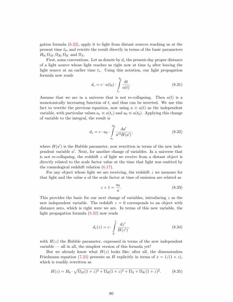
gation formula (6.22), apply it to light from distant sources reaching us at thepresent time t0, and rewrite the result directly in terms of the basic parametersH0,ΩM ,ΩR,ΩK and ΩΛ.

First, some conventions. Let us denote by de the present-day proper distanceof a light source whose light reaches us right now at time t0 after leaving thelight source at an earlier time te. Using this notation, our light propagationformula now reads

de = c · a(t0) ·t0∫te

dt

a(t). (8.31)

Assume that we are in a universe that is not re-collapsing. Then a(t) is amonotonically increasing function of t, and thus can be inverted. We use thisfact to rewrite the previous equation, now using a ≡ a(t) as the independentvariable, with particular values ae ≡ a(te) and a0 ≡ a(t0). Applying this changeof variable to the integral, the result is

de = c · a0 ·a0∫ae

da′

a′2H(a′), (8.32)

where H(a′) is the Hubble parameter, now rewritten in terms of the new inde-pendent variable a′. Next, for another change of variables. In a universe thatis not re-collapsing, the redshift z of light we receive from a distant object isdirectly related to the scale factor value at the time that light was emitted bythe cosmological redshift relation (6.17).

For any object whose light we are receiving, the redshift z we measure forthat light and the value a of the scale factor at time of emission are related as

z + 1 =a0

a. (8.33)

This provides the basic for our next change of variables, introducing z as thenew independent variable. The redshift z = 0 corresponds to an object withdistance zero, which is right were we are. In terms of this new variable, thelight propagation formula (8.32) now reads

de(z) = c ·z∫

0

dz′

H(z′), (8.34)

with H(z) the Hubble parameter, expressed in terms of the new independentvariable — all in all, the simplest version of this formula yet!

But we already know what H(z) looks like; after all, the dimensionlessFriedmann equation (7.23) presents us H explicitly in terms of x = 1/(1 + z),which is readily rewritten as

H(z) = H0 ·√

ΩM (1 + z)3 + ΩR(1 + z)4 + ΩΛ + ΩK(1 + z)2. (8.35)

80

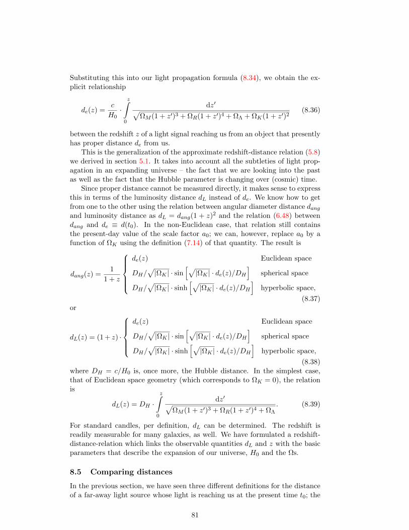
Substituting this into our light propagation formula (8.34), we obtain the ex-plicit relationship

de(z) =c

H0·

z∫0

dz′√ΩM (1 + z′)3 + ΩR(1 + z′)4 + ΩΛ + ΩK(1 + z′)2

(8.36)

between the redshift z of a light signal reaching us from an object that presentlyhas proper distance de from us.

This is the generalization of the approximate redshift-distance relation (5.8)we derived in section 5.1. It takes into account all the subtleties of light prop-agation in an expanding universe – the fact that we are looking into the pastas well as the fact that the Hubble parameter is changing over (cosmic) time.

Since proper distance cannot be measured directly, it makes sense to expressthis in terms of the luminosity distance dL instead of de. We know how to getfrom one to the other using the relation between angular diameter distance dangand luminosity distance as dL = dang(1 + z)2 and the relation (6.48) betweendang and de ≡ d(t0). In the non-Euclidean case, that relation still containsthe present-day value of the scale factor a0; we can, however, replace a0 by afunction of ΩK using the definition (7.14) of that quantity. The result is

dang(z) =1

1 + z

de(z) Euclidean space

DH/√|ΩK | · sin

[√|ΩK | · de(z)/DH

]spherical space

DH/√|ΩK | · sinh

[√|ΩK | · de(z)/DH

]hyperbolic space,

(8.37)or

dL(z) = (1 + z) ·

de(z) Euclidean space

DH/√|ΩK | · sin

[√|ΩK | · de(z)/DH

]spherical space

DH/√|ΩK | · sinh

[√|ΩK | · de(z)/DH

]hyperbolic space,

(8.38)where DH = c/H0 is, once more, the Hubble distance. In the simplest case,that of Euclidean space geometry (which corresponds to ΩK = 0), the relationis

dL(z) = DH ·z∫

0

dz′√ΩM (1 + z′)3 + ΩR(1 + z′)4 + ΩΛ

. (8.39)

For standard candles, per definition, dL can be determined. The redshift isreadily measurable for many galaxies, as well. We have formulated a redshift-distance-relation which links the observable quantities dL and z with the basicparameters that describe the expansion of our universe, H0 and the Ωs.

8.5 Comparing distances

In the previous section, we have seen three different definitions for the distanceof a far-away light source whose light is reaching us at the present time t0; the

81

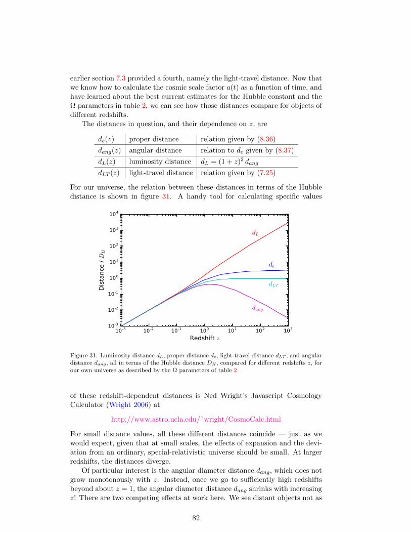
earlier section 7.3 provided a fourth, namely the light-travel distance. Now thatwe know how to calculate the cosmic scale factor a(t) as a function of time, andhave learned about the best current estimates for the Hubble constant and theΩ parameters in table 2, we can see how those distances compare for objects ofdifferent redshifts.

The distances in question, and their dependence on z, are

de(z) proper distance relation given by (8.36)

dang(z) angular distance relation to de given by (8.37)

dL(z) luminosity distance dL = (1 + z)2 dang

dLT (z) light-travel distance relation given by (7.25)

For our universe, the relation between these distances in terms of the Hubbledistance is shown in figure 31. A handy tool for calculating specific values

10-3 10-2 10-1 100 101 102 103

Redshift z

10-3

10-2

10-1

100

101

102

103

104

Dis

tance

/ D

H

dL

de

dLT

dang

Figure 31: Luminosity distance dL, proper distance de, light-travel distance dLT , and angulardistance dang, all in terms of the Hubble distance DH , compared for different redshifts z, forour own universe as described by the Ω parameters of table 2

of these redshift-dependent distances is Ned Wright’s Javascript CosmologyCalculator (Wright 2006) at

http://www.astro.ucla.edu/˜wright/CosmoCalc.html

For small distance values, all these different distances coincide — just as wewould expect, given that at small scales, the effects of expansion and the devi-ation from an ordinary, special-relativistic universe should be small. At largerredshifts, the distances diverge.

Of particular interest is the angular diameter distance dang, which does notgrow monotonously with z. Instead, once we go to sufficiently high redshiftsbeyond about z = 1, the angular diameter distance dang shrinks with increasingz! There are two competing effects at work here. We see distant objects not as

82

they are, but as they were in the past; in an expanding universe, any object inthe Hubble flow was closer to us in the past than it is now. By that reasoning,objects in the past should appear to have a larger angular diameter. On theother hand, there is basic geometry, namely that objects that are farther awayfrom us appear smaller, that is, have a smaller angular diameter. For objects atlower redshift, the latter effect dominates, while for more distant objects, theformer effect is dominant, leading to the unusual non-monotonous behaviourseen in figure 31.

9 The Redshift-distance diagram revisited

After a long journey through the concepts and calculations associated with anexpanding universe, we can return to our concrete goal of understanding Hubblediagrams, or more precisely: redshift-distance diagrams like our initial figure 1,which play a key role in comparing cosmological models with astronomicalobservations.

Let us collect the ingredients we need to understand that kind of diagram.We will, throughout, assume that we are in a Euclidean universe, ΩK = 0. Asdescribed in section 6.6, that particular property of the universe is best derivedusing another type of observations, namely fluctuations in the cosmic microwavebackground.

Consider standard candles, per definition of known luminosity L, whoseflux density I is measured by telescope observations. Our aim is to deduce asystematic relationship between those two quantities and the redshift of thelight we have received from a standard candle.

Once both L and I are known, we can deduce the object’s luminosity dis-tance dL, using the formula

I =L

4π d2L

. (6.55)

From our derivation in section 6.7, we know the relationship between luminositydistance and angular distance, and from the geometry section 6.6, we know thatin the special case of a Euclidean universe, angular distance is the same as theemitting object’s proper distance de from us, so that

dL ≡ de · (1 + ze), (6.54)

with ze the redshift we measure as the distant object’s light reaches us. Inan expanding universe, de and ze fulfill the redshift-distance relation (8.36).We neglect the radiation contribution ΩR which is only of interest in the veryearliest stages of cosmic history and whose absence will not markedly skewour picture; as already mentioned, we assume Euclidean space geometry, soΩK = 0, and we exploit the fact that for the remaining two density parameters,ΩΛ = 1−ΩM as per the present-day dimensionless Friedmann equation (7.26).

In consequence, for this special case, the redshift-distance relation takes on

83

the much simpler form

H0 · de = c ·ze∫

0

dz√ΩM (1 + z)3 − ΩM + 1

. ()

The only remaining complication is that astronomers will express the luminositydistance in terms of the distance modulus

µ(dL) ≡ 5 log10

(dL

10 pc

). (6.58)

All in all, we expect distance modulus µ and redshift ze of a distant standardcandle to be related by

µ = 5 log10

c

H0· 1

Mpc· (1 + ze) ·

ze∫0

dz√ΩM (1 + z)3 − ΩM + 1

+ 25. (9.1)

In practice, for supernovae, all the quantities inside the logarithm that are notdimensionless are separated, and lumped together with the absolute magnitude;the distance modulus is then fitted to supernova data as

µ = 5 log10

(1 + ze) ·ze∫

0

dz√ΩM (1 + z)3 − ΩM + 1

+ C, (9.2)

with two fit parameters: the ΩM we are interested in, and an offset C. Hadwe taken the more complicated formulae for more general geometries, we couldeven attempt to fit both ΩM and ΩΛ.

Figure 32 is our own version of the initial figure 1, using the same datafrom the Union 2.1 catalogue of the Supernova Cosmology Project, and fittingthe function (9.2): The link for downloading the data and the Python scriptfor fitting, and for producing figure 32, can be found in section A, p. 97f. Thefitted value of ΩM = 0.268 ± 0.025 is compatible with the result of the teamthat published the data, ΩM = 0.271± 0.014 (Suzuki et al. 2012).

10 Conclusions

While modern cosmological models are rooted in the framework of general rel-ativity, at least the simplified, homogeneous and isotropic expanding universecan be understood without recourse to the full formalism of Einstein’s theory.We have derived most of the formulae describing light propagation and thedynamics of the universal scale factor by going to small scales, making use ofthe equivalence principle and the Newtonian limit, taking care to arrive at ourresults in a way that allows generalisation to the universe as a whole – eitherby summing up infinitesimal contributions or because any exact local result forthe functional form of the scale factor a(t) automatically applies everywherethe scale factor is involved.

84

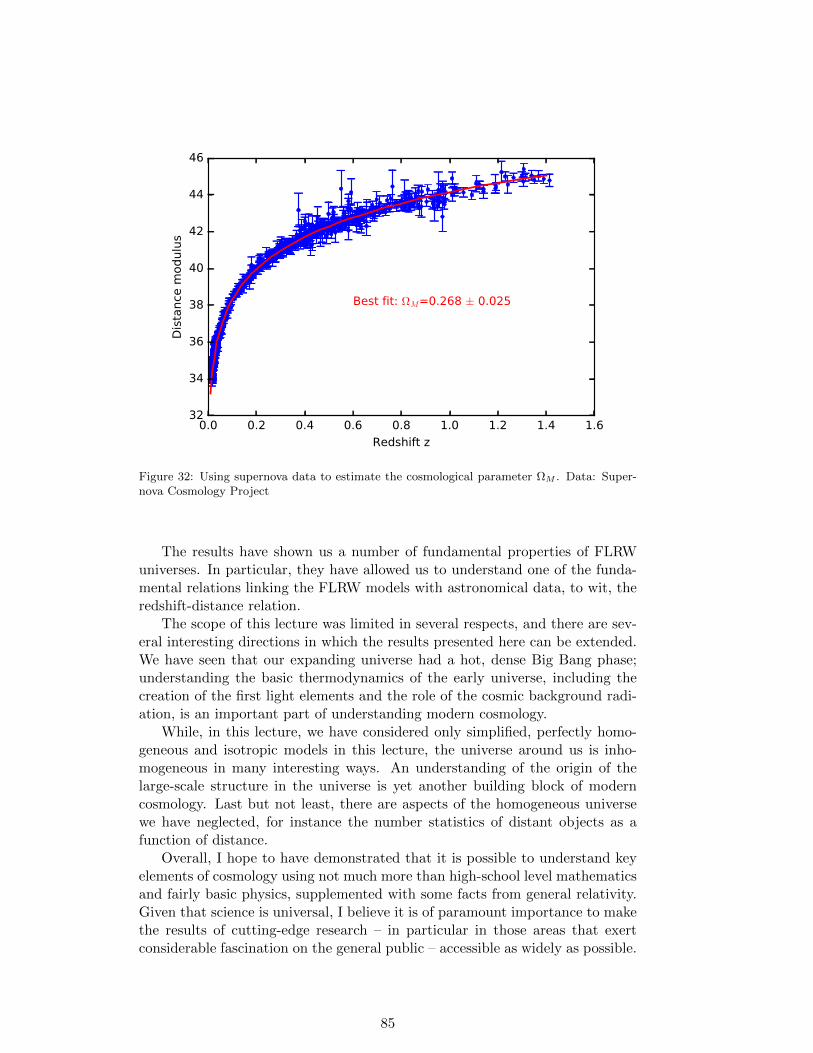
0.0 0.2 0.4 0.6 0.8 1.0 1.2 1.4 1.6

Redshift z

32

34

36

38

40

42

44

46

Dis

tance

modulu

s

Best fit: ΩM=0.268 ± 0.025

Figure 32: Using supernova data to estimate the cosmological parameter ΩM . Data: Super-nova Cosmology Project

The results have shown us a number of fundamental properties of FLRWuniverses. In particular, they have allowed us to understand one of the funda-mental relations linking the FLRW models with astronomical data, to wit, theredshift-distance relation.

The scope of this lecture was limited in several respects, and there are sev-eral interesting directions in which the results presented here can be extended.We have seen that our expanding universe had a hot, dense Big Bang phase;understanding the basic thermodynamics of the early universe, including thecreation of the first light elements and the role of the cosmic background radi-ation, is an important part of understanding modern cosmology.

While, in this lecture, we have considered only simplified, perfectly homo-geneous and isotropic models in this lecture, the universe around us is inho-mogeneous in many interesting ways. An understanding of the origin of thelarge-scale structure in the universe is yet another building block of moderncosmology. Last but not least, there are aspects of the homogeneous universewe have neglected, for instance the number statistics of distant objects as afunction of distance.

Overall, I hope to have demonstrated that it is possible to understand keyelements of cosmology using not much more than high-school level mathematicsand fairly basic physics, supplemented with some facts from general relativity.Given that science is universal, I believe it is of paramount importance to makethe results of cutting-edge research – in particular in those areas that exertconsiderable fascination on the general public – accessible as widely as possible.

85

11 Bibliography

Abbott, B. P. et al. (2017): “A gravitational-wave standard siren measure-ment of the Hubble constant”. In: Nature 551, pp. 85–88. doi: 10.1038/na-ture24471. arXiv: 1710.05835.

Adams, D. (1980): The Restaurant at the End of the Universe. Pan Books.isbn: 0-345-39181-0.

Adler, C. G. (1987): “Does mass really depend on velocity, dad?” In: AmericanJournal of Physics 55, pp. 739–743. doi: 10.1119/1.15314.

Baade, W. (1956): “The Period-Luminosity Relation of the Cepheids”. In:Proceedings of the Astronomical Society of the Pacific 68, pp. 5–16. doi:10.1086/126870.

Baez, J. C. and E. F. Bunn (2005): “The meaning of Einstein’s equation”.In: American Journal of Physics 73, pp. 644–652. doi: 10.1119/1.1852541.eprint: gr-qc/0103044.

Barnes, L. A. et al. (2006): “Joining the Hubble flow: implications for expand-ing space”. In: Monthly Notices of the Royal Astronomical Society 373, pp.382–390. doi: 10.1111/j.1365-2966.2006.11045.x. eprint: astro-ph/0609271.

Bennett, C. L. et al. (2013): “Nine-year Wilkinson Microwave AnisotropyProbe (WMAP) Observations: Final Maps and Results”. In: AstrophysicalJournal Supplement 208, 20., 20. doi: 10.1088/0067-0049/208/2/20. arXiv:1212.5225.

Bondi, H. (1960): Cosmology. Cambridge University Press.

Bondi, H. (1964): Relativity and Common Sense. A New Approach to Einstein.New York: Doubleday. isbn: 978-0486240213.

Bunn, E. F. and D. W. Hogg (2009): “The kinematic origin of the cosmo-logical redshift”. In: American Journal of Physics 77, pp. 688–694. doi:10.1119/1.3129103. arXiv: 0808.1081 [physics.pop-ph].

Caldwell, R. R., M. Kamionkowski, and N. N. Weinberg (2003): “PhantomEnergy: Dark Energy with w<-1 Causes a Cosmic Doomsday”. In: PhysicalReview Letters 91, 071301., 071301. doi: 10.1103/PhysRevLett.91.071301.eprint: astro-ph/0302506.

Callan, C., R. H. Dicke, and P. J. E. Peebles (1965): “Cosmology and New-tonian Mechanics”. In: American Journal of Physics 33, pp. 105–108. doi:10.1119/1.1971256.

Carrera, M. and D. Giulini (2010): “Influence of global cosmological expansionon local dynamics and kinematics”. In: Reviews of Modern Physics 82, pp.169–208. doi: 10.1103/RevModPhys.82.169. arXiv: 0810.2712 [gr-qc].

86

Clavering, W. J. (2006): “Comments on the tethered galaxy problem”. In:American Journal of Physics 74, pp. 745–750. doi: 10.1119/1.2203646.eprint: astro-ph/0511709.

Cooperstock, F. I., V. Faraoni, and D. N. Vollick (1998): “The Influence of theCosmological Expansion on Local Systems”. In: Astrophysical Journal 503,pp. 61–66. doi: 10.1086/305956. eprint: astro-ph/9803097.

Cornish, N. J., D. N. Spergel, and G. D. Starkman (1998): “Circles in the sky:finding topology with the microwave background radiation”. In: Classicaland Quantum Gravity 15, pp. 2657–2670. doi: 10.1088/0264-9381/15/9/013.eprint: gr-qc/9602039.

Davis, T. M., C. H. Lineweaver, and J. K. Webb (2003): “Solutions to thetethered galaxy problem in an expanding universe and the observation ofreceding blueshifted objects”. In: American Journal of Physics 71, pp. 358–364. doi: 10.1119/1.1528916. eprint: astro-ph/0104349.

Davis, T. M. (2005): “Fundamental aspects of the expansion of the universeand cosmic horizons”. PhD dissertation, Australia: University of New SouthWales (Australia). Publication Number: AAT 0807562. DAI-B 66/01, Jul2005. eprint: astro-ph/0402278.

de Bernardis, P. et al. (2000): “A flat Universe from high-resolution maps ofthe cosmic microwave background radiation”. In: Nature 404, pp. 955–959.doi: 10.1038/35010035. eprint: astro-ph/0004404.

de Grijs, R. (2011): An introduction to distance measurement in astronomy.Chichester: Wiley. isbn: 978-0-470-51180-0.

de Sitter, W. (1917): “On the relativity of inertia. Remarks concerning Ein-stein’s latest hypothesis”. In: Koninklijke Nederlandse Akademie van Weten-schappen Proceedings Series B Physical Sciences 19, pp. 1217–1225.

d’Inverno, R. (1992): Introducing Einstein’s Relativity. Oxford University Press.isbn: 978-0198596868.

Earman, J. (1995): Bangs, Crunches, Whimpers, and Shrieks - Singularitiesand Acausalities in Relativistic Spacetimes. Oxford University Press. isbn:9780195095913.

Eddington, A. S. (1930): “On the instability of Einstein’s spherical world”.In: Monthly Notices of the Royal Astronomical Society 90, pp. 668–678. doi:10.1093/mnras/90.7.668.

Ehlers, J., I. Ozsvath, and E. L. Schucking (2006): “Active mass un-der pressure”. In: American Journal of Physics 74, pp. 607–613. doi:10.1119/1.2198881. eprint: gr-qc/0505040.

Einstein, A. (1917): “Kosmologische Betrachtungen zur allgemeinen Rela-tivitatstheorie”. In: Sitzungsberichte der Koniglich Preußischen Akademieder Wissenschaften (Berlin), pp. 142–152.

87

Fraknoi, A. (1995): The Universe at Your Fingertips. An Astronomy Activityand Resource Notebook. Project Astro at the Astronomical Society of thePacific. isbn: 978-1886733008.

Freedman, W. L. et al. (2001): “Final Results from the Hubble Space TelescopeKey Project to Measure the Hubble Constant”. In: Astrophysical Journal 553,pp. 47–72. doi: 10.1086/320638. eprint: astro-ph/0012376.

Friedmann, A. (1922): “Uber die Krummung des Raumes”. In: Zeitschrift furPhysik 10, pp. 377–386. doi: 10.1007/BF01332580.

Friedmann, A. (1924): “Uber die Moglichkeit einer Welt mit konstanter neg-ativer Krummung des Raumes”. In: Zeitschrift fur Physik 21, pp. 326–332.doi: 10.1007/BF01328280.

Fukugita, M. and P. J. E. Peebles (2004): “The Cosmic Energy Inventory”.In: Astrophysical Journal 616, pp. 643–668. doi: 10.1086/425155. eprint:astro-ph/0406095.

Gausmann, E. et al. (2001): “Topological lensing in spherical spaces”. In:Classical and Quantum Gravity 18, pp. 5155–5186. doi: 10.1088/0264-9381/18/23/311. eprint: gr-qc/0106033.

Giulini, D. (2014): “Does cosmological expansion affect local physics?” In:Studies in the History and Philosophy of Modern Physics 46, pp. 24–37. doi:10.1016/j.shpsb.2013.09.009. arXiv: 1306.0374 [gr-qc].

Grøn, Ø. and Ø. Elgarøy (2007): “Is space expanding in the Friedmann uni-verse models?” In: American Journal of Physics 75, pp. 151–157. doi:10.1119/1.2360990. eprint: astro-ph/0603162.

Harrison, E. (2000): Cosmology. The science of the universe. Cambridge Uni-versity Press. isbn: 978-0521661485.

Hawking, S. W. and G. F. R. Ellis (1973): The large-scale structure of space-time. Cambridge University Press.

Hecht, E. (2009a): “Einstein on mass and energy”. In: American Journal ofPhysics 77, pp. 799–806. doi: 10.1119/1.3160671.

Hecht, E. (2009b): “Einstein Never Approved of Relativistic Mass”. In: ThePhysics Teacher 47, pp. 336–341. doi: 10.1119/1.3204111.

Hogg, D. W. et al. (2002): “The K correction”. In: ArXiv Astrophysics e-printseprint: astro-ph/0210394.

Hoyle, F. (1954): “Protocol of session 28, “Commission des nebuleuses extra-galactiques”. In: Transactions of the International Astronomical Union Vol.8. Ed. by Oosterhoff, P. Th. Wiley, pp. 297–299.

Hubble, E. (1929): “A Relation between Distance and Radial Velocity amongExtra-Galactic Nebulae”. In: Proceedings of the National Academy of Science15, pp. 168–173. doi: 10.1073/pnas.15.3.168.

88

Jagannathan, K. (2009): “Momentum due to pressure: A simple model”. In:American Journal of Physics 77, pp. 432–433. doi: 10.1119/1.3081105.

Jarrett, T. H. et al. (2000): “2MASS Extended Source Catalog: Overviewand Algorithms”. In: Astronomical Journal 119, pp. 2498–2531. doi:10.1086/301330. eprint: astro-ph/0004318.

Jordan, T. F. (2005): “Cosmology calculations almost without generalrelativity”. In: American Journal of Physics 73, pp. 653–662. doi:10.1119/1.1900095. eprint: astro-ph/0309756.

Krauss, L. M. and G. D. Starkman (2000): “Life, the Universe, and Nothing:Life and Death in an Ever-expanding Universe”. In: Astrophysical Journal531, pp. 22–30. doi: 10.1086/308434. eprint: astro-ph/9902189.

Leavitt, H. S. (1908): “1777 variables in the Magellanic Clouds”. In: Annals ofHarvard College Observatory 60, pp. 87–108.3.

Leibundgut, B. et al. (1996): “Time Dilation in the Light Curve of the DistantType IA Supernova SN 1995K”. In: Astrophysical Journal Letters 466, L21.doi: 10.1086/310164. eprint: astro-ph/9605134.

Lemaıtre, G. (1927): “Un Univers homogene de masse constante et derayon croissant rendant compte de la vitesse radiale des nebuleuses extra-galactiques”. In: Annales de la Societe Scientifique de Bruxelles 47, pp. 49–59.

Lemaıtre, G. (1931a): “The Beginning of the World from the Point of View ofQuantum Theory.” In: Nature 127, 706. doi: 10.1038/127706b0.

Lemaıtre, G. (1931b): “L’Expansion de l’Espace”. In: Publications du Labora-toire d’Astronomie et de Geodesie de l’Universite de Louvain 8, pp. 101–120.

Liebscher, D.-E. (2005): The Geometry of Time. Wiley VCH. isbn: 978-3-527-40567-1.

Liske, J. et al. (2008): “Cosmic dynamics in the era of Extremely Large Tele-scopes”. In: Monthly Notices of the Royal Astronomical Society 386, pp.1192–1218. doi: 10.1111/j.1365-2966.2008.13090.x. arXiv: 0802.1532.

Lotze, K.-H. (1995): “Special and general relativity and cosmology for teachersand high-school students”. In: Thinking physics for teaching. Ed. by Bernar-dini, C., C. Tarsitani, and M. Vincentini. New York: Plenum Press, pp.335–354.

Lotze, K.-H. (2002): “Das Weltmodell der Newtonschen Kosmologie”. In:Wege in der Physikdidaktik Band 5: Naturphanomene und Astronomie. Ed.by Lotze, K.-H. and W. B. Schneider. Erlangen & Jena: Palm & Enke,pp. 238–249. url: http://www.solstice.de/cms/upload/wege/band5/

wege5-238-249.pdf

89

Maxwell, J. C. (1873): A Treatise on Electricity and Magnetism, Vol. 2.Oxford: Clarendon Press. url: http://catalogue.bnf.fr/ark:/12148/

cb30914055c

McCrea, W. H. (1955): “Newtonian Cosmology”. In: Nature 175, 466. doi:10.1038/175466a0.

McCrea, W. H. and E. A. Milne (1934): “Newtonian Universes and the curva-ture of space”. In: The Quarterly Journal of Mathematics 5, pp. 73–80. doi:10.1093/qmath/os-5.1.73.

Mermin, N. D. (2005a): It’s about time : understanding Einstein’s relativity.Princeton, NJ: Princeton University Press. isbn: 978-0691122014.

Mermin, N. D. (2005b): “From Einstein’s 1905 postulates to the geome-try of flat space-time”. In: Annalen der Physik 517, pp. 103–114. doi:10.1002/andp.200410122. eprint: gr-qc/0411069.

Milne, E. A. (1934): “A Newtonian expanding Universe”. In: The QuarterlyJournal of Mathematics 5, pp. 64–72. doi: 10.1093/qmath/os-5.1.64.

Misner, C. W. and P. Putnam (1959): “Active Gravitational Mass”. In: PhysicalReview 116, pp. 1045–1046. doi: 10.1103/PhysRev.116.1045.

Narlikar, J. V. (1994): “Spectral shifts in general relativity”. In: AmericanJournal of Physics 62, pp. 903–907. doi: 10.1119/1.17679.

Okun, L. B. (1989): “The concept of mass”. In: Physics Today 42, pp. 31–46.doi: 10.1063/1.881171.

Okun, L. B. (2009): “Mass versus relativistic and rest masses”. In: AmericanJournal of Physics 77, pp. 430–431. doi: 10.1119/1.3056168.

Ono, Y. A. (1982): “How I created the theory of relativity”. In: Physics Today35, pp. 45–48. doi: 10.1063/1.2915203.

Pachner, J. (1963): “Mach’s Principle in Classical and Relativistic Physics”.In: Physical Review 132, pp. 1837–1842. doi: 10.1103/PhysRev.132.1837.

Pachner, J. (1964): “Nonconservation of Energy During Cosmic Evolution”. In:Physical Review Letters 12, pp. 117–118. doi: 10.1103/PhysRevLett.12.117.

Patrignani, C. and Particle Data Group (2016): “Review of ParticlePhysics”. In: Chinese Physics C 40, 100001., 100001. doi: 10.1088/1674-1137/40/10/100001. url: http://pdg.lbl.gov/

Peacock, J. A. (2002): “An introduction to the physics of cosmology”. In:Modern Cosmology. Ed. by Bonometto, S., V. Gorini, and U. Moschella.Oxford University Press, pp. 9–107.

Perlmutter, S. et al. (1997): “Cosmology From Type IA Supernovae: Measure-ments, Calibration Techniques, and Implications”. In: American Astronom-ical Society Meeting Abstracts. Wiley, 1351. eprint: astro-ph/9812473.

90

Peters, P. C. (1986): “An alternate derivation of relativistic momentum”. In:American Journal of Physics 54, pp. 804–808. doi: 10.1119/1.14450.

Planck Collaboration (2016): “Planck 2015 results. XIII. Cosmological pa-rameters”. In: Astronomy & Astrophysics 594, A13. doi: 10.1051/0004-6361/201525830. arXiv: 1502.01589.

Possel, M. (2010a): “Time dilation on the road”. In: Einstein Online 4, 1006.url: http://www.einstein-online.info/spotlights/time_dilation_

road

Possel, M. (2010b): “Twins on the road”. In: Einstein Online 4, 1008. url:http://www.einstein-online.info/spotlights/time_dilation_road

Possel, M. (2017): “‘Teaching cosmology with special relativity: Piecewise in-ertial frames as a model for cosmic expansion”. In preparation.

Poisson, E. (2014): Gravity: Newtonian, Post-Newtonian, Relativistic. Cam-bridge: Cambridge University Press. isbn: 978-1107032866.

Price, R. H. and E. Grover (2001): “Cosmological expansion in the classroom”.In: American Journal of Physics 69, pp. 125–128. doi: 10.1119/1.1287354.

Price, R. H. and J. D. Romano (2012): “In an expanding universe, whatdoesn’t expand?” In: American Journal of Physics 80, pp. 376–381. doi:10.1119/1.3699245.

Riazuelo, A. et al. (2004): “Simulating cosmic microwave background mapsin multiconnected spaces”. In: Physical Review D 69, 103514. doi:10.1103/PhysRevD.69.103514. eprint: astro-ph/0212223.

Riess, A. G. et al. (2016): “A 2.4% Determination of the Local Value of theHubble Constant”. In: Astrophysical Journal 826, 56. doi: 10.3847/0004-637X/826/1/56. arXiv: 1604.01424.

Rindler, W. (1977): Essential Relativity. Special, General and Cosmological.Springer. isbn: 978-3-540-07970-5.

Rindler, W. et al. (1990): “Putting to Rest Mass Misconceptions”. In: PhysicsToday 43, 13. doi: 10.1063/1.2810555.

Robertson, H. P. (1927): “Dynamical space-times which contain a conformalEuclidean 3-space”. In: Transactions of the American Mathematical Society29, pp. 481–496. doi: 10.1090/S0002-9947-1927-1501400-9.

Rohrlich, F. (1990): “An elementary derivation of E=mc2”. In: American Jour-nal of Physics 58, pp. 348–349. doi: 10.1119/1.16168.

Sandin, T. R. (1991): “In defense of relativistic mass”. In: American Journalof Physics 59, pp. 1032–1036. doi: 10.1119/1.16642.

Schild, A. (1960): “Equivalence Principle and Red-Shift Measurements”. In:American Journal of Physics 28, pp. 778–780. doi: 10.1119/1.1936000.

91

Schroter, U. (2002): “Allgemeine Relativitatstheorie mit den Mitteln der Schul-mathematik”. In: Wege in der Physikdidaktik Band 5: Naturphanomene undAstronomie. Erlangen & Jena: Palm & Enke, pp. 174–187. url: http:

//www.solstice.de/cms/upload/wege/band5/wege5-p2-174-187.pdf

Schutz, B. F. (1985): A first course in general relativity. Cambridge: CambridgeUniversity Press. isbn: 978-0521887052.

Schutz, B. F. (1986): “Determining the Hubble constant from gravitationalwave observations”. In: Nature 323, 310. doi: 10.1038/323310a0.

Schutz, B. F. (2004): Gravity from the Ground Up. Cambridge: CambridgeUniversity Press. isbn: 978-0521455060.

Strauss, M. A. (2016): “The Expansion of the Universe”. In: Welcome to theUniverse. Ed. by Tyson, N. D., M. A. Strauss, and J. R. Gott. PrincetonUniversity Press, Ch. 14

Suzuki, N. et al. (2012): “The Hubble Space Telescope Cluster Supernova Sur-vey. V. Improving the Dark-energy Constraints above z > 1 and Buildingan Early-type-hosted Supernova Sample”. In: Astrophysical Journal 746, 85.doi: 10.1088/0004-637X/746/1/85. arXiv: 1105.3470 [astro-ph.CO].

Trimble, V. (2013): “Anybody but Hubble!” arXiv: 1307.2289 [physics.hist-ph].

Udalski, A. et al. (1999): “The Optical Gravitational Lensing Experiment.Cepheids in the Magellanic Clouds. III. Period-Luminosity-Color and Period-Luminosity Relations of Classical Cepheids”. In: Acta Astronomica 49, pp.201–221. eprint: astro-ph/9907236.

Visser, M. (2004): “Jerk, snap and the cosmological equation of state”. In:Classical and Quantum Gravity 21, pp. 2603–2615. doi: 10.1088/0264-9381/21/11/006. eprint: gr-qc/0309109.

Walker, A. G. (1935): “On Riemannian spaces with spherical symmetry about aline, and the conditions for isotropy in general relativity”. In: The QuarterlyJournal of Mathematics 6, pp. 81–93. doi: 10.1093/qmath/os-6.1.81.

Weinberg, S. (2008): Cosmology. Oxford University Press.

Wheeler, J. A. (1990): A Journey into Gravity and Spacetime. W. H. Freeman& Co Ltd. isbn: 978-0716750161.

Whiting, A. B. (2004): “The expansion of space: free-particle motion and thecosmological redshift”. In: The Observatory 124, pp. 174–189. eprint: astro-ph/0404095.

Wright, E. L. (2006): “A Cosmology Calculator for the World Wide Web”. In:Proceedings of the Astronomical Society of the Pacific 118, pp. 1711–1715.doi: 10.1086/510102. eprint: astro-ph/0609593.

92

Index

ΛCDM models, 68Ω parameters (density), 55

values, 672MASX catalogue, 16

absolute magnitude, 51absorption lines, 26age of the universe, 64angular diameter distance, 48apparent brightness, 29apparent magnitude, 50arc length, 47astronomical unit, 27atoms

and cosmic expansion, 74attached galaxy problem, 76axion, 72

Baade, Walter, 31baryonic matter, 68Big Bang, 62Big Bang nucleosynthesis, 68Big Bang phase, 62Big Bang singularity, 62Big Crunch, 64Big Rip, 77Bondi, Hermann, 17bound systems

and cosmic expansion, 70–77

Carter-Penrose diagram, 63Cartesian coordinates, 97Cepheid variables, 27charge

elementary, 74closed universe, 58co-moving clock

galaxy, 22cold dark matter, 68conformal diagram, 63constant

cosmological, 37coordinate system

in special relativity, 97Copernican principle, 17

cosmic background radiation, 49, 63,68, 69

cosmic expansion, 19–20and bound systems, 70–77

cosmic scale factor, 19dynamics, 51–54

cosmic time, 22cosmological constant, 37cosmological parameter values, 67cosmological principle, 17cosmological redshift, 26, 38

as Doppler shift, 40cosmology, 4

Newtonian, 51Coulomb force, 74critical density, 55

and space geometry, 58value, 67

curvature, 6

dark energy, 55constant density, 37equation of state, 36

dark matter, 68dark matter particles, 72de Sitter solution, 66de Sitter universe

event horizon, 70de Sitter, Willem, 66deceleration parameter, 34density

change due to expansion, 36, 37critical, 55

distanceangular diameter, 48Hubble, 26light-travel, 57luminosity, 50proper, 20

distance ladder, 27distance modulus, 51Doppler effect, 26

classical, 102special-relativistic, 103transverse, 103

93

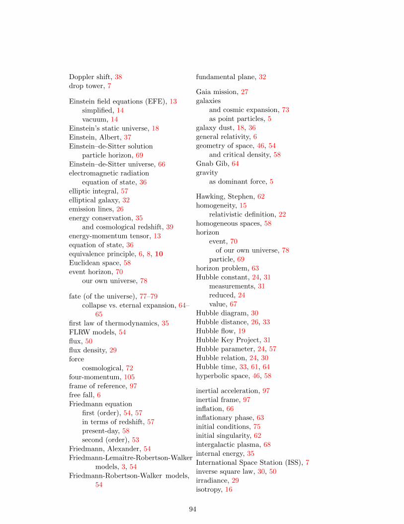
Doppler shift, 38drop tower, 7

Einstein field equations (EFE), 13simplified, 14vacuum, 14

Einstein’s static universe, 18Einstein, Albert, 37Einstein–de-Sitter solution

particle horizon, 69Einstein–de-Sitter universe, 66electromagnetic radiation

equation of state, 36elliptic integral, 57elliptical galaxy, 32emission lines, 26energy conservation, 35

and cosmological redshift, 39energy-momentum tensor, 13equation of state, 36equivalence principle, 6, 8, 10Euclidean space, 58event horizon, 70

our own universe, 78

fate (of the universe), 77–79collapse vs. eternal expansion, 64–

65first law of thermodynamics, 35FLRW models, 54flux, 50flux density, 29force

cosmological, 72four-momentum, 105frame of reference, 97free fall, 6Friedmann equation

first (order), 54, 57in terms of redshift, 57present-day, 58second (order), 53

Friedmann, Alexander, 54Friedmann-Lemaıtre-Robertson-Walker

models, 3, 54Friedmann-Robertson-Walker models,

54

fundamental plane, 32

Gaia mission, 27galaxies

and cosmic expansion, 73as point particles, 5

galaxy dust, 18, 36general relativity, 6geometry of space, 46, 54

and critical density, 58Gnab Gib, 64gravity

as dominant force, 5

Hawking, Stephen, 62homogeneity, 15

relativistic definition, 22homogeneous spaces, 58horizon

event, 70of our own universe, 78

particle, 69horizon problem, 63Hubble constant, 24, 31

measurements, 31reduced, 24value, 67

Hubble diagram, 30Hubble distance, 26, 33Hubble flow, 19Hubble Key Project, 31Hubble parameter, 24, 57Hubble relation, 24, 30Hubble time, 33, 61, 64hyperbolic space, 46, 58

inertial acceleration, 97inertial frame, 97inflation, 66inflationary phase, 63initial conditions, 75initial singularity, 62intergalactic plasma, 68internal energy, 35International Space Station (ISS), 7inverse square law, 30, 50irradiance, 29isotropy, 16

94

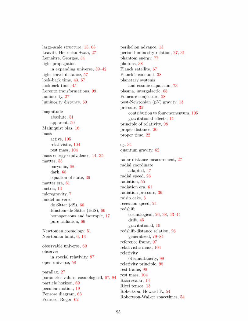
large-scale structure, 15, 68Leavitt, Henrietta Swan, 27Lemaıtre, Georges, 54light propagation

in expanding universe, 39–42light-travel distance, 57look-back time, 43, 57lookback time, 45Lorentz transformations, 99luminosity, 27luminosity distance, 50

magnitudeabsolute, 51apparent, 50

Malmquist bias, 16mass

active, 105relativistic, 104rest mass, 104

mass-energy equivalence, 14, 35matter, 55

baryonic, 68dark, 68equation of state, 36

matter era, 61metric, 13microgravity, 7model universe

de Sitter (dS), 66Einstein–de-Sitter (EdS), 66homogeneous and isotropic, 17pure radiation, 66

Newtonian cosmology, 51Newtonian limit, 6, 13

observable universe, 69observer

in special relativity, 97open universe, 58

parallax, 27parameter values, cosmological, 67, 84particle horizon, 69peculiar motion, 19Penrose diagram, 63Penrose, Roger, 62

perihelion advance, 13period-luminosity relation, 27, 31phantom energy, 77photons, 38Planck satellite, 67Planck’s constant, 38planetary systems

and cosmic expansion, 73plasma, intergalactic, 68Poincare conjecture, 58post-Newtonian (pN) gravity, 13pressure, 35

contribution to four-momentum, 105gravitational effects, 14

principle of relativity, 98proper distance, 20proper time, 22

q0, 34quantum gravity, 62

radar distance measurement, 27radial coordinate

adapted, 47radial speed, 26radiation, 55radiation era, 61radiation pressure, 36raisin cake, 3recession speed, 24redshift

cosmological, 26, 38, 43–44drift, 45gravitational, 10

redshift-distance relation, 26generalized, 79–84

reference frame, 97relativistic mass, 104relativity

of simultaneity, 99relativity principle, 98rest frame, 98rest mass, 104Ricci scalar, 13Ricci tensor, 13Robertson, Howard P., 54Robertson-Walker spacetimes, 54

95

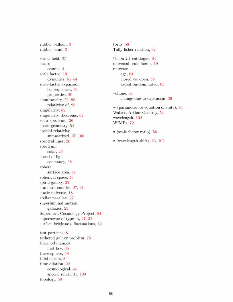
rubber balloon, 3rubber band, 3

scalar field, 37scales

cosmic, 4scale factor, 19

dynamics, 51–54scale-factor expansion

consequences, 34properties, 20

simultaneity, 22, 98relativity of, 99

singularity, 62singularity theorems, 62solar spectrum, 26space geometry, 54special relativity

summarized, 97–106spectral lines, 26spectrum

solar, 26speed of light

constancy, 98sphere

surface area, 47spherical space, 46spiral galaxy, 32standard candles, 27, 31static universe, 18stellar parallax, 27superluminal motion

galaxies, 25Supernova Cosmology Project, 84supernovae of type Ia, 27, 32surface brightness fluctuations, 32

test particles, 8tethered galaxy problem, 75thermodynamics

first law, 35three-sphere, 58tidal effects, 8time dilation, 22

cosmological, 44special relativity, 100

topology, 58

torus, 58Tully-fisher relation, 32

Union 2.1 catalogue, 84universal scale factor, 19universe

age, 64closed vs. open, 58radiation-dominated, 65

volume, 35change due to expansion, 36

w (parameter for equation of state), 36Walker, Arthur Geoffrey, 54wavelength, 102WIMPs, 72

x (scale factor ratio), 56

z (wavelength shift), 26, 102

96

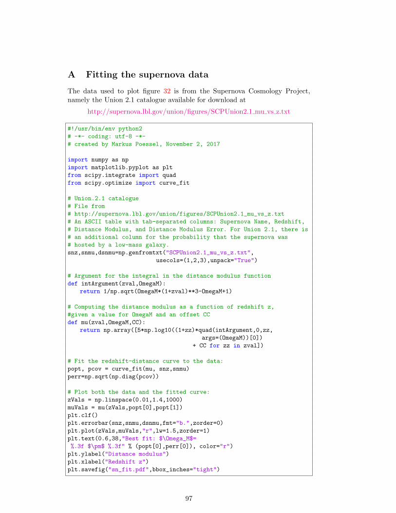
A Fitting the supernova data

The data used to plot figure 32 is from the Supernova Cosmology Project,namely the Union 2.1 catalogue available for download at

http://supernova.lbl.gov/union/figures/SCPUnion2.1 mu vs z.txt

#!/usr/bin/env python2

# -*- coding: utf-8 -*-

# created by Markus Poessel, November 2, 2017

import numpy as np

import matplotlib.pyplot as plt

from scipy.integrate import quad

from scipy.optimize import curve_fit

# Union.2.1 catalogue

# File from

# http://supernova.lbl.gov/union/figures/SCPUnion2.1_mu_vs_z.txt

# An ASCII table with tab-separated columns: Supernova Name, Redshift,

# Distance Modulus, and Distance Modulus Error. For Union 2.1, there is

# an additional column for the probability that the supernova was

# hosted by a low-mass galaxy.

snz,snmu,dsnmu=np.genfromtxt("SCPUnion2.1_mu_vs_z.txt",

usecols=(1,2,3),unpack="True")

# Argument for the integral in the distance modulus function

def intArgument(zval,OmegaM):

return 1/np.sqrt(OmegaM*(1+zval)**3-OmegaM+1)

# Computing the distance modulus as a function of redshift z,

#given a value for OmegaM and an offset CC

def mu(zval,OmegaM,CC):

return np.array([5*np.log10((1+zz)*quad(intArgument,0,zz,

args=(OmegaM))[0])

+ CC for zz in zval])

# Fit the redshift-distance curve to the data:

popt, pcov = curve_fit(mu, snz,snmu)

perr=np.sqrt(np.diag(pcov))

# Plot both the data and the fitted curve:

zVals = np.linspace(0.01,1.4,1000)

muVals = mu(zVals,popt[0],popt[1])

plt.clf()

plt.errorbar(snz,snmu,dsnmu,fmt="b.",zorder=0)

plt.plot(zVals,muVals,"r",lw=1.5,zorder=1)

plt.text(0.6,38,"Best fit: $\Omega_M$=

%.3f $\pm$ %.3f" % (popt[0],perr[0]), color="r")

plt.ylabel("Distance modulus")

plt.xlabel("Redshift z")

plt.savefig("sn_fit.pdf",bbox_inches="tight")

97

B What we need from special relativity

In order to make these lecture notes more accessible, I briefly summarize here anumber of statements from special relativity that are used in the main text. Itshould be clear, however, that this brief version can be no more than a crutch— the best option for interested readers not familiar with special relativity isto change that state of affairs by reading books such as Mermin 2005a. In themain text, the equivalence principle, cf. section 3.1, plays an important role.In brief, that principle states that for an observer in free fall in a gravitationalfield described by Einstein’s general theory of relativity, the laws of physicsare (approximately) the same as those of special relativity. So what are thepertinent laws of special relativity?

B.1 Inertial reference frames

For the usual description of moving particles (and more complex objects), youneed a frame of reference. Most commonly, you describe particle positions byintroducing a Cartesian coordinate system, defined in just the right way so thatcoordinate distances correspond to physical distances, as measured with a ruleror more modern measuring device. In classical physics, one usually does notthink too much about introducing a time coordinate. Time is a parameter thatdescribes how change happens within your system; ideal clocks divide time upinto unit intervals, one second the same as the next, one hour the same as anyother. (The latter is easily said; linking it to actual measurements is tricky,though — how can you tell that a clock is ideal?)

In some reference frames, if you let a particle drift, making sure that noneof the known forces such as gravity or electromagnetism exert any significantinfluence, such free particles will nevertheless be seen to accelerate, and in asystematic way: If you track their motions, you will be able to separate acceler-ation into a component that acts on all particles in the same way, a componentthat depends on the distance from a certain line in space (the rotation axis),a component that depends on the velocity component orthogonal to that sameline, and a component orthogonal both to the line and to the particle’s directiontoward that line. These are linear, centrifugal, Coriolis, and Euler acceleration,respectively, jointly known as inertial accelerations.

A reference frame in which these inertial accelerations are absent, and freeparticles move at constant speeds along straight lines, is called an inertial frame.These are the most common frames used in classical mechanics, even though areference frame at rest relative to the Earth’s surface – to name a very commonexample – is only approximately inertial, seeing that the Earth itself is a rotatingreference frame.

The nomenclature regarding inertial frames or, more general, reference frames,varies; the terms “frame,” “reference frame,” “frame of reference,” “observer”and “coordinate system” are used fairly interchangeably. The rationale,presumably, is that each observer will have defined a personal reference frame(that is, a frame in which the observer is at rest) to record their observations,and that descriptions within a given reference frame are made in terms of space

98

and time coordinates. The elementary concept in such a setting is an event,defined as something identifiable happening at a specific location in space, at aspecific point in time. (And yes, this is an idealization — just like the conceptof a space point is an idealization.)

An inertial frame in which an object is at rest is often called that object’srest frame.

B.2 Relativity principle and constant light speed

Einstein’s special theory of relativity posits that there is such a thing as inertialframes, and that the following two principles hold:

1. Principle of relativity: the laws of physics have the same simple formin every inertial frame.

2. Constancy of the speed of light: the speed of light in vacuum has thesame value in each inertial frame. In particular, it does not depend onthe motion of the light source.

Inertial frames can be in constant motion relative to each other; the first prin-ciple states that, when it comes to the laws of physics, no inertial frame isdistinguished from any other. This is in contrast to earlier notions of an abso-lute space, which set a standard of absolute rest.

The expression “the same simple form” refers to physical laws linking spe-cific quantities. Assume, for instance, that the energy E and momentum p ofa massless particle are linked as E = pc, with c the (vacuum) speed of light,in one inertial frame, that is: with the energy E and momentum p measuredin that specific frame. Then the same form holds in any other inertial frame,as well: the energy E′ and momentum p′ as measured in such another inertialframe are, again, linked, as E′ = p′c. The energy-momentum-relation has thesame mathematical form in all inertial frames.

A direct consequence of the principle of relativity is that, if you set up aparticular experiment in one inertial frame, and then set up the same experi-ment in another inertial frame, the results will be the same. There is no way ofdistinguishing between inertial frames using local experiments — that is, exper-iments that are defined solely within an inertial frame, and do not include anyoutside influences. (A counter-example would be two different inertial frames inone and the same external magnetic field; unless the magnetic field were to haveexactly the same properties in both inertial frames, local magnetic experimentsin each frame would not be equivalent.)

We will make use of the constancy of the speed of light when we describelight propagation in an expanding universe in section 6.3.

The constancy of the speed of light is directly linked to notions of simul-taneity. Einstein’s definition of simultaneity of two events is as follows. Imaginean observer who is at rest in the chosen reference frame S, and who is locatedhalf-way between the locations of two events (in other words: if we join the twolocations by a straight line, then the distance between our observer and the firstevent location will be the same as the observer’s distance to the second event

99

location, with all distances measured in the inertial frame S). Now imagine thatdirectly at each event, a light signal is sent from the event location towards ourobserver. The two events in question are simultaneous as defined in the inertialframe S if and only if these two light signals arrive at the half-way observer atthe same time. It is a key property of special relativity that with this defini-tion, simultaneity is relative: two events that are simultaneous in one inertialsystem S are not, in general, simultaneous in another inertial system S′ if thosetwo systems are in relative motion.

With an (ideal) master clock, at rest in a specific inertial frame, and specificlight signals, we can chart that reference frame’s spacetime geometry: We canmeasure distances by the travel time of a reflected light signal (as in radardistance ranging). And we can find the time coordinate value (vulgo “thetime”) to assign to an event as follows, in a variation of the above definitionof simultaneity: if a light signal leaves our master clock at t = T1, reaches thelocation of the event E at just the time the event is happening, is reflected andarrives back at the master clock at time t = T2, then the event E was happeningat time

t(E) =T1 + T2

2. (B.1)

In this way, one can reconstruct the whole of the geometry of space and time, asdefined by special relativity (Mermin 2005b, Liebscher 2005). This approach,using radar coordinates and what has become known as the k-calculus, waspioneered by Hermann Bondi (Bondi 1964).

B.3 Transformations

Clearly, the constancy of the speed of light is incompatible with classical me-chanic’s recipe of relating two reference frames in relative motion. In classicalmechanics, relative velocities add up directly. If a spaceship is chasing a lightsignal, and if we, in our reference frame, see the light signal moving at speedc and the spaceship at speed v, both in the same direction, we would deducethat, for an observer in the spaceship, the light signal would move at the re-duced speed c − v. This is contradicted by the principle of the constancy ofthe speed of light. Clearly, the transition between one inertial reference frameand another is somewhat more complicated in special relativity than in classicalmechanics.

We will not go into detail about the Lorentz transformations, that is, aboutthe formulae defining the transition from one inertial frame to another in specialrelativity. It is worth mentioning, however, that they link space and time insuch a way that it makes more sense to talk about the set of all events in spaceand time, in short: about four-dimensional spacetime.

There is a helpful analogy that makes use of our usual notion of space. Wecan introduce an x, y and z axis in order to describe three-dimensional space.If we rotate the resulting coordinate system, space will still be the same, butthe x, y and z directions are now different. Thus, it makes no sense to take thedivision into x, y and z too seriously – much more important is the underlyingthree-dimensional structure. In the same way, the Lorentz transformations show

100

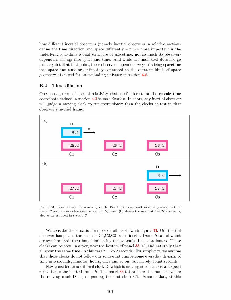
how different inertial observers (namely inertial observers in relative motion)define the time direction and space differently – much more important is theunderlying four-dimensional structure of spacetime, not so much its observer-dependant slicings into space and time. And while the main text does not gointo any detail at that point, these observer-dependent ways of slicing spacetimeinto space and time are intimately connected to the different kinds of spacegeometry discussed for an expanding universe in section 6.6.

B.4 Time dilation

One consequence of special relativity that is of interest for the cosmic timecoordinate defined in section 4.3 is time dilation. In short, any inertial observerwill judge a moving clock to run more slowly than the clocks at rest in thatobserver’s inertial frame.

26.2

C1

8.1

Dv

26.2

C2

26.2

C3

27.2

C1

8.6

Dv

27.2

C2

27.2

C3

(a)

(b)

Figure 33: Time dilation for a moving clock. Panel (a) shows matters as they stand at timet = 26.2 seconds as determined in system S; panel (b) shows the moment t = 27.2 seconds,also as determined in system S

We consider the situation in more detail, as shown in figure 33: Our inertialobserver has placed three clocks C1,C2,C3 in his inertial frame S, all of whichare synchronized, their hands indicating the system’s time coordinate t. Theseclocks can be seen, in a row, near the bottom of panel 33 (a), and naturally theyall show the same time, in this case t = 26.2 seconds. For simplicity, we assumethat those clocks do not follow our somewhat cumbersome everyday division oftime into seconds, minutes, hours, days and so on, but merely count seconds.

Now consider an additional clock D, which is moving at some constant speedv relative to the inertial frame S. The panel 33 (a) captures the moment wherethe moving clock D is just passing the first clock C1. Assume that, at this

101

particular moment, the moving clock D is showing the time 8.1 seconds on itsdisplay.

The situation one second later (as determined in the inertial system S) isshown in the panel 33 (b). Apparently, clock placement happens to be suchthat one second was all it took for clock D to move from the location of C1 tothat of C3, so we see the moment where D passes C3. The fact that, in thesystem S, one second has passed, is dutifully recorded by the three clocks atrest in S, which now show t = 27.2 seconds.

But when we compare D with the clock C3 (easily done since both are atthe same location at that particular moment), we see that D is now showing8.7 seconds. On clock D, only half a second has passed between the two panels.In this sense, clock D is running more slowly than clocks C1, C2 and C3. Inour specific example, D has been running only half as fast as C1, C2,C3.

For this situation, the relation between a time interval ∆t as shown by clocksthat are synchronized in S and the time interval ∆t′ shown by the moving clockD, which is moving at speed v relative to the inertial system S, is given by

∆t′ = ∆t ·√

1− (v/c)2, (B.2)

where c is the speed of light (in vacuum). From the fact that, in our example,∆t′ = 0.5 ·∆t, we can deduce that clock D must have been moving at the speedv =

√3/4 c ≈ 0.866 c.

A key result of special relativity is that time dilation is mutual. We canturn the tables: Clock D is at rest in a suitable inertial system, which wecan call S′. In this system, we can introduce additional clocks D2, D3, whichare synchronized to the system’s time coordinate t′. We can line the threesynchronized clocks up in a row so that each of C1, C2, C3 passes by D, D2 andD3. In that situation, a direct comparison of each of the C clocks with the Dclocks along the line will give the result that, compared with a row of D clocks,the C clock is going more slowly!

How can each set of clocks be slower than the other? This is resolved onceon realizes that each judgement involves a standard of comparison, namely anotion of simultaneity — and that simultaneity is not the same in the restframe of the C clocks and the D clocks. In fact, there is a simple analogyusing the geometry of the two-dimensional plane that shows how the apparentcontradiction is resolved (Possel 2010a;b).

In the context of cosmological models, the fact that clocks in relative motionmeasure time differently is mainly important as a warning, showing us that thecosmic time coordinate introduced in section 4.3 is unusual, and certainly notthe usual time coordinate used in, say, classical mechanics.

B.5 Doppler effect

The basics of the Doppler effect are well-known from classical mechanics. Fromthe point of view of an inertial observer, the maxima and minima of a lightwave will move at the speed of light; for a light source moving away from suchan observer, this makes for longer wavelengths than for a source that is at restrelative to the observer.

102

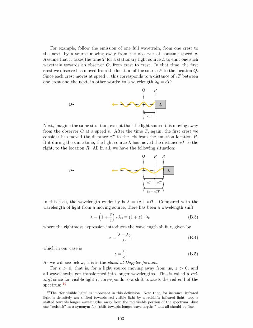
For example, follow the emission of one full wavetrain, from one crest tothe next, by a source moving away from the observer at constant speed v.Assume that it takes the time T for a stationary light source L to emit one suchwavetrain towards an observer O, from crest to crest. In that time, the firstcrest we observe has moved from the location of the source P to the location Q.Since each crest moves at speed c, this corresponds to a distance of cT betweenone crest and the next, in other words: to a wavelength λ0 = cT :

O

cT

PQ

L

Next, imagine the same situation, except that the light source L is moving awayfrom the observer O at a speed v. After the time T , again, the first crest weconsider has moved the distance cT to the left from the emission location P .But during the same time, the light source L has moved the distance vT to theright, to the location R! All in all, we have the following situation:

O

cT

PQ R

L

vT

(c+ v)T

In this case, the wavelength evidently is λ = (c + v)T . Compared with thewavelength of light from a moving source, there has been a wavelength shift

λ =(

1 +v

c

)· λ0 ≡ (1 + z) · λ0, (B.3)

where the rightmost expression introduces the wavelength shift z, given by

z ≡ λ− λ0

λ0, (B.4)

which in our case isz =

v

c. (B.5)

As we will see below, this is the classical Doppler formula.For v > 0, that is, for a light source moving away from us, z > 0, and

all wavelengths get transformed into longer wavelengths. This is called a red-shift since for visible light it corresponds to a shift towards the red end of thespectrum.19

19The “for visible light” is important in this definition. Note that, for instance, infraredlight is definitely not shifted towards red visible light by a redshift; infrared light, too, isshifted towards longer wavelengths, away from the red visible portion of the spectrum. Justuse “redshift” as a synonym for “shift towards longer wavelengths,” and all should be fine.

103

For v < 0, one can make a similar argument, but this time the light sourcewould be moving towards the observer. We would find z < 0, so all wavelengthsget shorter. This is called a blueshift, since for visible light it corresponds to ashift towards the blue end of the spectrum.

But there is still one factor we have left out. Our time T , correspondingto the period of the light, was measured in our own reference frame. But asrecounted in section B.4, time dilation means that the period T ′ determined byan observer on the light source will actually be shorter, namely

T ′ = T ·√

1− (v/c)2. (B.6)

The corresponding wavelength of the light, as measured by an observer at restrelative to the light source, will be λ′ = cT ′. In classical physics, where allspeeds are much slower than that of light, v c, this effect is negligible, andwe do end up with the classical Doppler formula (B.5). But once we take intoaccount (B.6), we find that

λ = (c+ v) · T =(c+ v) T ′√1− (v/c)2

=(1 + v/c) cT ′√

(1 + v/c)(1− v/c)=

√1 + v/c

1− v/cλ′ (B.7)

corresponding to

z =λ− λ′

λ′=

√1 + v/c

1− v/c− 1. (B.8)

This is the (longitudinal) special-relativistic Doppler effect. Note that, as thespeed of the source approaches the speed of light, v → c, the wavelength shiftz grows beyond all bounds.

There is also a transverse special-relativistic Doppler effect, although thatwill not play a role in our cosmological considerations. In case a light source ismoving neither towards us nor away from us, but transversally, namely at rightangles to our line of sight (equivalently: to the direction of light propagation),there will still be a wavelength shift due to time dilation alone – by (B.6), wehave

λ = cT =cT ′√

1− (v/c)2=

λ′√1− (v/c)2

(B.9)

for the wavelength λ′ as measured at the light source and the wavelength λ asmeasured by an inertial observer relative to whom the light source is movingtransversally at the speed v.

B.6 E = mc2

Perhaps the most famous consequence of special relativity is Einstein’s formulaE = mc2, the equivalence of mass and energy. It can be derived by applyingthe formulae of special-relativistic mechanics to e.g. simple collisions (Peters1986, Rohrlich 1990). As a first step, one finds that an increase ∆E in energyfor an object, or system, will necessarily result in an equivalent increase ∆m inthe inertial mass, that is, in the mass factor that determines how strongly an

104

object will react to an external force by accelerating. That relativistic (inertial)mass relates velocity ~v and momentum ~p in an inertial system,

~p = m · ~v, (B.10)

and is involved in linking the force ~F acting on an object and the change inmomentum experienced by that object as

~F =d~p

dt. (B.11)

For an object moving at a speed v in an inertial reference frame, the relativisticmass is

m =m0√

1− (v/c)2, (B.12)

where m0 is the rest mass, that is, the relativistic mass as measured in aninertial frame in which that object is at rest.

With this definition of mass, E = mc2 states that mass and energy areequivalent: one cannot have energy without inertial mass, or inertial masswithout a corresponding energy. Both physical concepts turn out to measurethe same quantity; the only difference is one of units (as is shown by the requiredconversion factor c2).

There is an alternative way of looking at things, which identifies the conceptof mass with the rest mass m0, and omits mention of the relativistic inertialmass as defined by (B.10) as far as possible, if not altogether. In that case, onewould rewrite the momentum definition as

~p =m0√

1− (v/c)2· ~v, (B.13)

and keep the v-dependent extra factor (which is known as the gamma factor) ex-plicit. In that context, Einstein’s famous formula describes not an equivalence,but an additional form of energy: the energy

E0 = m0c2 (B.14)

associated with an object’s rest mass; whenever one is talking about energyconservation, this extra form of energy needs to be taken into account. A newform of energy entails new forms of energy conversion: rest mass energy can beconverted into other forms of energy, such as electromagnetic energy, or thermalenergy.

These two different ways of talking about mass – mass as relativistic mass,or mass as rest mass – have led to intense discussions in the physics educationcommunity over the past decades, e.g. Adler 1987, Rindler et al. 1990, Sandin1991, Okun 1989; 2009, Hecht 2009a;b. I would argue that, given the state ofthat discussion, a good working knowledge of special relativity should includean awareness of both views of the matter, and of the controversy itself.

105

B.7 Energy, momentum, and pressure

As mentioned in section B.3, time and space, as described using inertial frames,are really two aspects of a four-dimensional entity called spacetime. Analo-gously, as it turns out, energy and momentum are really just two aspects of afour-dimensional vector, called four-momentum.

In relativistic theories that respect this four-dimensional structure, it doesnot make sense to formulate equations, say, that single out only energy, andleave momentum aside. Such an equation will only hold for certain inertialobservers, but not for others (in the language of relativity, they are not covari-ant); this is at odds with the relativity principle which states that any physicallaw should have the same form in all inertial frames. So why not choose thatparticular form to describe physics in the first place?

Whenever we formulate equations that are valid in any inertial referenceframe, energy and momentum will always occur together, or in the shape offour-momentum.

This has consequences when, at a more advanced level, namely in generalrelativity, we try to find the proper way of describing the mass/energy contentof the universe: finding the right physical concept to describe sources of rela-tivistic gravity, in other words: the active mass in general relativity. How do wedescribe the mass/energy content of a universe filled with, say, a gas consistingof particles, or of photons, whizzing chaotically in every conceivable direction?The first generalization is straightforward. Instead of merely considering themass directly associated with matter, we will consider all forms of energy assources of gravity. That is why, in section 3.5 on the generalization of Newton’sequation of gravity, our density ρ will include all kinds of energy contributions(equivalently: will be the density of the relativistic mass introduced in sectionB.6).

But even with that addition, we are not yet fully relativistic. After all,energy and momentum cannot be separated from each other in an observer-independent way; if energy is a source of gravity, momentum must be a sourceterm as well. For a gas made of particles, we will get not only a contributionfrom all these particles’ rest masses, kinetic energy and so on, but also fromthe particle momenta. When the momenta only describe the chaotic motion ofa gas that is, on average, at rest, then these momentum contributions turn outto be directly proportional to the pressure p exerted by the gas. That is why,in section 3.5, there is a contribution 3p/c2: a pressure contribution, convertedinto the proper units of a mass density via the factor c2, with one contributionfrom each of the three space directions.20

A simple derivation of the pressure contribution to the momentum densitycan be found in Jagannathan 2009; for a more complete understanding, oneneeds to understand both four-vectors and the tensor description of the prop-

20Interestingly enough, while this pressure term is important in cosmology, there is a com-plication in the situation where we are closest to our everyday notion of what pressure is, thatis, when we are looking at a gas inside a container with suitable walls. There, the stress expe-rienced by the walls exactly cancels the contribution from the 3p/c2 term of the gas (Misnerand Putnam 1959, Ehlers, Ozsvath, and Schucking 2006).

106

erties of a fluid or similar medium; a good introduction can be found in Schutz1985.

Acknowledgements

The summer school “Astronomy from Four Perspectives” from August 26 toSeptember 2 in Heidelberg, at which this lecture was held, was made possiblethrough generous funding from the W. E. Heraeus Foundation.

I would like to thank Thomas Muller for his thorough and, in parts, repeatedreading of this manuscript and his many corrections and suggestions; I wouldalso like to thank Martin Wetz, Bjorn Malte Schafer and Stefan Brems forhelpful comments and useful suggestions concerning previous versions of thismanuscript.

107