the evolution of inequality in mexico: 1895-1940

EKHM51

Master’s Thesis (15 credits ECTS)

June 2019

Supervisor: Erik Bengtsson

Examiner: Andrés Palacio

Word Count: 15,574

Master’s Programme in Economic Growth, Population and Development

[Economic History Track]

The Evolution of Inequality in Mexico: 1895-1940

by

Diego Castañeda Garza

[email protected]

Abstract

The evolution of inequality in Latin America, particularly in Mexico, is a topic of growing

interest among economists, economic historians and policy makers. For the Mexican case, this

study empirically estimates, for the first time, the evolution of Mexican inequality before 1950.

This thesis produces a new database and employs it to construct social tables for four

benchmark years, 1895,1910,1930 and 1940. The evidence points to inequality being a political

phenomenon; inequality levels change as policies change. Over the long run, the evolution of

inequality displays a strong persistence. The results are in line with a new branch of the

literature that identifies the importance of land ownership for inequality dynamics. The study

of the evolution of inequality in this period contributes to derive valuable lessons from

developing countries with large agrarian populations and challenge some of the dominant

theories of inequality.

Keywords: Income Inequality, Social Tables, Mexico, Mexican Revolution.

ii

Acknowledgements

In writing this paper, I have come to collect considerable debts to several individuals and

institutions who advised me, supported me or lend me their eyes and their minds for reading,

commenting and discussing my research.

First, I would like to acknowledge the Swedish Institute and their staff for the funding they

provided me during my studies in Sweden; this would not be possible without their generosity.

Second, to Lund University and the Department of Economic History for delivering an

engaging intellectual environment in which thinking becomes much easier. Finally, to the

National Institute of Statistics, Geography and Information (INEGI) for their help gaining

access to old data sources.

A special acknowledge is deserved by my supervisor, professor Erik Bengtsson, whose

comments and advise improved the quality of my arguments. I would also like to thank

Professor Javier Rodríguez Weber, who guided me in the early stages of developing this project

and suggested ways to improve my measurements. Also, for all the trouble I caused at class by

asking question after question about the reconstruction of old data, a recognition is necessary

for professor Jutta Bolt.

I want to thank Gabriela Astorga, Ana Corzo and Kaj Löfgren for reading several drafts of this

work and suggesting ways to improve its readability. Also, to Sergio Silva Castañeda, Luis

Angel Monroy Gómez Franco and Raúl Zepeda from the economist group of Democracia

Deliberada for their exciting ideas and discussions about inequality and economic history in

Mexico, and to my friends Diego Alejo Vázquez for his comments on my data reconstruction

procedures and Raoul Herbert for all the entertaining and enlighted discussion over the year.

Last but not least, I wish to thank my parents Gabino Castañeda Cárdenas and María Antonieta

Garza Aguilar for their absolute support, confidence and their lessons in the value of history.

Finally, to Sarahí Panecatl Martínez whose encouragement and love kept the winter at bay.

iii

Table of Contents 1 Introduction ...................................................................................................................... 1

1.1 Why Mexico? ............................................................................................................. 1

1.2 Research Problem ....................................................................................................... 3

1.3 Research Questions .................................................................................................... 4

2 Literature Review ............................................................................................................. 7

2.1 Theories of Inequality ................................................................................................ 7

2.2 Historical Inequality Studies of Mexico ..................................................................... 9

3 Data, Sources and Methods ........................................................................................... 12

3.1 Social Tables ............................................................................................................ 12

3.2 The 1895 and 1910 Social Tables ............................................................................ 14

3.3 The 1930 and 1940 Social Tables ............................................................................ 20

3.4 From Social Tables to the Lorenz Curves and the Gini Index ................................. 29

4 Results ............................................................................................................................. 30

4.1 Summary of Results ................................................................................................. 30

4.2 The Evolution of Mexican Income Inequality ......................................................... 30

4.3 History is the rock upon which economic theories survive or are broken ............... 46

5 Conclusions and Further Discussion ............................................................................ 49

5.1 Inequality as a Political Choice ................................................................................ 49

5.2 Persistent Inequality? ............................................................................................... 53

References ............................................................................................................................... 56

Archival and Statistical Sources ........................................................................................... 56

Articles and Books ............................................................................................................... 60

Appendix A: Social Tables Construction and Alternative Measurements. ...................... 69

Appendix B: Alternative 1930 Social Table ......................................................................... 72

Appendix C: Code and Data ................................................................................................. 78

iv

List of Tables

Table 1: 1895 Social Table (rounded numbers) ..................................................................... 18

Table 2: 1910 Social Table (rounded numbers) .................................................................... 19



Table 5: Mexico's inequality (Gini index) 1895,1910,1930 and 1940................................... 30

Table 6: Strikes and resolutions 1920-1936 ........................................................................... 39

Table 7: Incomes and ratios between occupational groups, Mexican pesos ........................ 44

Table 8: 1930 Social Table: within inequality robustness check (rounded num.) ............... 72

Table 9: Comparison 1930 (Table 3) vs 1930 (Table 8) ......................................................... 77

v

List of Figures

Figure 1: Winners and losers: real gains by occupational group 1895-1910...................... 34

Figure 2: Mexico's Lorenz curves 1895 & 1910 min max levels ......................................... 36

Figure 3: Mexico's Lorenz curves 1895 min max levels. ..................................................... 36


Figure 5: Winners and losers: real gains by selected occupational groups 1930-1940 ...... 42

Figure 6: Mexico's Lorenz curves 1930 & 1940 min max levels. ........................................ 43



Figure 9: The evolution of inequality in Mexico: 1895-2016 .............................................. 50

Figure 10: The vicious cycle of inequality ............................................................................ 55

Figure 11: Examples of aggregated occupational categories. ............................................. 69

Figure 12: Relative winners and losers by occupational categories 1895-1910. ................. 70

Figure 13: Relative winners and losers by selected occupational categories 1930-1940. ... 70

1

1 Introduction

1.1 Why Mexico?

Latin America is arguably the most unequal region in the world and Mexico is one of the most

unequal countries. Mexico, a Spanish colony for three centuries and an independent country for

the following two, provides an important case for the study of inequality. Mexico is the second

most populated country in the region and the second-biggest economy. It has the second highest

per capita income and is arguably one of the most unequal, if not the most unequal country in

several measurements. For example, it has one of the highest shares of concentrated income

and wealth at the top 1 per cent of the distribution, close to 22 per cent (Esquivel, 2015) and

female participation in the labour market is among the lowest with just 45 per cent (OECD).

The debate on whether Latin American countries’ high degree of inequality go back to the

colonialism of the sixteenth century and its extractive institutions (Sokoloff & Engerman 1997;

Acemoglu, Johnson & Robinson 2001, 2002), or if it has a more recent origin. Some economic

historians argue that the origins of present day Latin American inequality are in late nineteenth

century commodity booms exports (Williamson 2010, 2015; Dobado, 2010). In this view, it is

the ownership of natural resources like silver, oil and some agricultural production the factors

that constitute the primary source behind the region high inequality levels.

A study of Mexico, besides its importance by itself, can also contribute to the general debate

on historical inequality. It becomes relevant to state that Mexico was partially industrialised in

the late nineteenth century, which according to the industrialisation-dominated literature

(Kuznets, 1955) should lead to increasing inequality. The country also experienced a political

and social revolution at the beginning of the twentieth century; the Mexican Revolution

arguably had distributional effects as the modern inequality literature theorises (Acemoglu,

Robinson & Johnson, 2001, 2002; Piketty, 2014; Scheidel, 2017). Furthermore, it produced the

first constitution that incorporated social and labour rights; the Constitution of 1917 and a post-

revolutionary regime trapped in a fragile equilibrium. For all its bloodshed, the revolution left

untouched most of the industrial apparatus of the Porfirian era, and with them, a large part of

2

the economic elite. Simultaneously, the new regime had the substantial compromise of

improving living standards, redistribute land and a more inclusive political agenda, which

allowed the lower social classes to get a seat at the table. Keeping this equilibrium would be

one of the central tenets of the nationalist post-revolutionary regime and a driver of the

development process over the twentieth century.

To study the evolution of inequality we construct social tables for the benchmark years of

1895,1910,1930 and 1940. These are the first comprehensive inequality estimates for Mexico

before year 1950. The construction of social tables is a method which proceeds by combining

income estimates for social groups, with information about each group’s share of the population

from censuses. This is the standard approach in economic history studies of inequality (Lindert

& Williamson, 2016; Gómez de León & De Jong, 2018). By using this approach, we can

provide new inequality estimates for the years 1895-1940, a turbulent period in Mexican

history. These benchmark years encompass the formative period of the modern Mexican state,

a time that forged the economic, political and social life of modern Mexico. It allows us to trace

the evolution of inequality between the Porfirio Díaz’s dictatorship during the last decades of

the nineteenth century, to the consolidation of the post-revolutionary Mexico near the end of

the first half of the twentieth century.

This thesis will contribute to the existing economic and economic history literature of inequality

by providing, for the first time, estimates for the level and trend of Mexican inequality of

income between 1895 and 1940. It will contribute to the discussion on the relevance of the most

prominent theories about inequality by calling into question their adequacy and providing an

alternative view of the mechanisms that drive inequality, particularly the relevance of land

ownership in understanding inequality dynamics. Moreover, it contributes to the policy

discussion of inequality reduction by exploring the political economy of Mexico and its

relevance for countries going through an industrialisation process today. Its final contribution

is to show that Mexico’s political economy and the specific policies introduced throughout the

1895-1940 period produced different levels of inequality, as well as producing different sets of

winners and losers. It will show that the Mexican Revolution was a pathway that created, for a

brief period, the conditions for a more egalitarian society. Thus, this thesis will argue that the

level of inequality is a political choice and not a necessary feature of economic development.

3

Although the primary focus of this research is quantitative, it will heavily rely on history to

interpret the data whenever a contextual analysis is required. The thesis will demonstrate that

neither of the main theories for the origins of inequality in the continent, the inherited

institutions one, nor the Kuznets hypothesis or commodity booms exports and others, can

explain on their own the phenomenon of the Mexican inequality over the end of the nineteenth

century and the first half of the twentieth. It will present that inequality was not constant; it

changed as policies changed.

1.2 Research Problem

The study of inequality in historical context is of special importance for the current

understanding of inequality. The dynamics of inequality take time to fully develop, the hard

swings in the distribution of income are often difficult to observe in the short term but become

more evident over the long run. In that sense, to understand inequality through time we require

to adopt the frame of mind of those who study “social time”, that is the evolution of the

structures of society (Braudel, 1976).

In a world in which inequality is a concern at national and global levels, case studies like the

Mexican one are valuable sources of knowledge to aid us in understanding the circumstances

that produce changes in the levels of inequality. Today, developing countries can learn from

the experience of other developing countries. Researchers that wish to study this evolution can

find in historical inequality studies tools to ponder upon the main theories that attempt to

explain the causes and cures for inequality and its consequences.

In the light of history, it is possible to test the validity of theory, the possibilities for

generalisation and the special cases that enrich our understanding. Mexican history provides us

with an opportunity to see these inequality theories in action. The historical inequality literature

in the world points to several channels through which the income distribution suffers changes,

nonetheless, not all countries’ histories are well-suited for the dominant explanations.

In addition to contributing to the inequality debate around the world, Mexico is an important

case of study because it is one of the largest developing countries in the world, both in the size

of its population and the size of its economy; it has a rich history and a prevailing complicated

4

political environment. Moreover, Mexican historical inequality is not well known, studies tend

to focus on recent decades due to the accessibility to reliable income statistics. Therefore, the

levels of inequality that prevailed before 1950 remain unexplored. At the same time, the

Porfiriato (the 30 years of Porfirio Díaz rule), the Mexican Revolution and the start of the post-

revolutionary regime are among the most studied periods in the non-inequality literature. Given

that the literature focuses substantially on living standards, economic conditions and the links

of those to political and social events, not having an actual account of inequality levels before

1950 results in a serious void of information that limits the understanding of the periods.

Ensuing from this discussion, the research problem of this thesis is to establish the relationship

between existent inequality levels and social, political and economic changes experienced over

the end of the nineteenth century and the first half of the twentieth.

1.3 Research Questions

This thesis will attempt to answer the following questions related to the evolution of inequality:

a) What was the level of inequality from the late porfiriato to post-revolutionary

Mexico, 1895-1940?

b) Can inequality be explained by structural change forces alone? Alternatively,

could it be the result of the political-economy process?

c) Did the Mexican Revolution produce a change in the levels of inequality? Moreover,

if it changed, through which channels?

d) Did the agrarian reform lead to higher incomes among the agrarian population and

thus had impact in the inequality levels?

e) Did the introduction of labour and social rights lead to higher wages and thus had

influence in the inequality levels?

What is the logic behind questions a) and b)?

Nineteenth century Mexico was predominantly an agrarian society, for that reason the primary

driver of income was the ownership of land and the resources associated with it, minerals like

gold and silver and agricultural output (Wilkie, 1990; Turchin & Nefedov, 2009). It had a

5

disconnected economy due to geographical factors, lack of infrastructure and the prevalence of

artisan manufacturing (Haber, 1989). Also, the unstable political environment promoted

backwardness. As a poor agrarian country, it is logical to expect low levels of inequality. Not

much surplus income could be extracted from the vast majority of the population. Though,

economic elites, particularly at regional level, because of the lack of state capacity, could have

taken extraction to the possible maximum (Milanovic, 2006; Milanovic, 2011; Milanovic,

Lindert & Williamson, 2011).

At the end of the nineteenth century things started to change. An industrialisation process

started to take place during the last two decades of the century, under the Porfirio Díaz’s

government. This process takes a form closely related to that described by Alexander

Gerschenkron in his masterful work, Economic Backwardness in Historical Perspective. An

economic and political elite colluded to take the driving seat in the economy, ensuring

monopoly rents, protection from international trade and preventing the organisation of workers

(Haber 1989; Kuntz, 2002; Beatty, 2002; Bortz, 2002; Haber, 2002). This political and

economic structure combined with the strong economic growth from the period, most certainly

produced an increase in the levels of inequality.

The trend the social tables reveal about the levels of inequality can expose the answer to this

alleged evolution. Either the evolution was more Kuznetsian, related to a Smithian growth take

off, or more Gerschenkronian, intertwined with rents, political power, inappropriate

technologies in capital intensity and scale, repression and exploitation

What is the logic behind questions c), d) and e)?

The Mexican Revolution, a byproduct of the collapse of the delicate institutional equilibrium

of the Porfirian regime is a perfect case to assess one of the more recently prominent

hypotheses, the reduction of inequality through history by means of the destruction produced

by wars and revolutions (Turchin, 2007; Turchin & Nefedov, 2009; Scheidel, 2017). According

to this view, violence is often a malign source of levelling. Popular beliefs or even misguided

myths about the Mexican Revolution argue that the Revolution was not only chaotic, it brought

large-scale destruction of the productive economic apparatus. Nevertheless, what most of the

historiography shows is that in terms of lives it was extremely costly, but in terms of physical

capital and its owners, it left them untouched. Could it be then that this great levelling force

was absent?

6

An alternative way of viewing the levelling produced by the Revolution is to consider the

effects of the new Constitution. The 1917 Constitution, conceived by the Revolution, was the

first in the world to introduce social rights (González de Aragón, 2017), among them the rights

to education and healthcare, labour rights and the ownership of the nation over its natural

resources. In turn, these new set of rights had an impact on policies that over time transformed

the country. At the same time, the new regime found that if it wanted to appease the country at

the revolution aftermath, major land reform was needed, and state capacity required to be built.

Consequently, these motivated policy changes such as new taxes, the creation of the “ejido” as

a communal property right instrument and mechanisms for workers to create political pressure

like legalised strikes and labour rights. These mechanisms have impact on inequality (Piketty

& Saez, 2003; Piketty, 2014) and partly depend on elite convenience (Acemoglu, Robinson &

Johnson, 2001). The more detailed social tables that can be constructed from 1930 and onwards,

make the exploration of those channels feasible.

Why focus on this period? Those years would see the development of most of the structural

transformations experienced over the last hundred years, which are in tension with the changes

implemented from the 1980s forwards. A tension that is reemerging as Mexico’s new

government looks towards the past for positive experiences that can be replicated. The second

reason is practical as fortuitously, enough data exists to reconstruct occupational groups, wages

and some other forms of earnings. The present works constructs a new dataset of those

variables. Finally, the Mexican experience is not due to its exceptionalism and is in many ways

familiar to how current developing countries are industrialising and how some did through

history. This research will add knowledge to the existing literature improving our understanding

of the development process in this type of setting and its effects around the world.

7

2 Literature Review

2.1 Theories of Inequality

Several competing theories can explain the changes in the income distribution. First, we have

the long-time workhorse of inequality studies, the Kuznets hypothesis (Kuznets, 1955), which

relates inequality to the process of economic development.

Kuznets argued that as a country develops, moving from agrarian societies with traditional

economic sectors towards industrial societies with modern economic sectors, inequality would

increase. Then after some level of development is attained, inequality should decrease as

development continues. The full relationship takes the shape of an inverse U. The Kuznets

hypothesis is often taken as an argument for considering inequality as a normal by-product of

the economic development process in a society.

With the expansion of the inequality studies around the world over the last decade, the Kuznets

hypothesis has been questioned. A plethora of studies show developed countries with rising

levels of inequality, this fact challenges Kuznets as these countries’ inequality levels decreased

decades ago and then rose again. Leading the critic of Kuznets ideas, we find the work of Piketty

and Saez (2003), Alvaredo, Atkinson, Piketty and Saez (2013), Piketty (2014) for a series of

developed countries with decreasing and then increasing inequality. Milanovic, Lindert and

Williamson (2011), Álvarez del Nogal and Prados de la Escosura (2013), Milanovic (2016),

showing us what is now called “Kuznets waves”. Gómez de León and De Jong (2018) and

Bengtsson, Missiaia, Nummela and Olsson (2018), documenting for Germany and for Finland

that inequality follows a different behaviour than those theorised by Kuznets (1955).

A competing mechanism for the Kuznets hypothesis is Piketty’s formulation of r>g, popularised

in his book Capital in the Twenty-First Century and recently supported by the work of Jordà,

Knoll, Kuvshinov, Schularick, and Taylor (Forthcoming). The r>g theory suggests that the

return of capital in a broader definition is, during normal circumstances, greater than the rate of

economic growth. This relationship implies that the owners of capital can accumulate wealth

and assets at a faster rate than the population, which can only rely on wages and salaries

8

typically tied to the overall performance of the economy, also known as the rate of economic

growth. If this mechanism is mainly at play, we should observe that the income of the owners

of capital rises faster than wages and skews the distribution upwards. A relevant side of this

theory of inequality is the relationship between capital owners and the political process, to

paraphrase Adam Smith (2004[1776], p.32) quoting Thomas Hobbes, wealth is power, and

wealth has the tendency to use that power to keep accumulating.

Another competing theory that shares with Piketty the relationship with political power, is the

new institutional approach. The Work of Engerman and Sokoloff (1997, 2012) and Acemoglu,

Robinson and Johnson (2001, 2002) argue that the existence of extractive institutions explains

inequality. The new institutionalists argue that the levels of inequality in present time Latin

America can be traced back to the colonial period under the Portuguese and Spanish empires,

an inheritance that can explain the high levels of inequality we observe to this day. There is no

dispute, the colonial past had enormous influence in countries development paths; path

dependency is a real thing. However, these types of arguments have been criticised from

different approaches. First, by the standing position of the Latin American ECLAC school

(Cardoso & Falleto, 1967) because it simplifies the existent political economy relating to whom,

under what circumstances and for what purposes institutions can be used to obtain returns.

Second, it has been criticised empirically by Williamson (2010, 2015) and Dobado (2010)

because when measuring inequality in colonial times employing the social tables from

Milanovic, Lindert and Williamson (2011) inequality was not significantly different in Latin

American than in other regions of the world. Instead they consider that inequality can be traced

back to the commodity boom exports of the late nineteenth century.

Finally, another approach to explaining inequality has been proposed by Scheidel (2017) in his

book The Great Leveler. Scheidel argues that through history, inequality has only been reduced

in a significant way by what he calls the negative forces of levelling: famine, war, plague and

revolution. This hypothesis suggests that inequality decreases at a high cost, for example,

through the destruction of capital in the First and Second world wars, the massive loss of life

consequence of the Black Death or the revolutionary violence seen in the Russian and Chinese

Revolutions, which included lofty radical agrarian reforms. The evidence from World War I

and World War II and the subsequent compression of the income distribution in Europe and the

United States back this hypothesis. The evidence of compression in the after wars period is

plenty, it can be found in Piketty and Saez (2003), Alvaredo, Atkinson, Piketty and Saez (2013),

9

Piketty (2014), Milanovic (2016) and Jordà, Knoll, Kuvshinov, Schularick, and Taylor

(Forthcoming).

No single theory can explain the evolution of inequality in every country and at every time.

Inequality as a social phenomenon is highly dependent in context. Specific patterns, empirical

regularities and relationships might hold through time, but they are not physical laws, the

evolution of inequality responds to changing circumstances. Finding what mechanism explains

the specific evolution one is looking at is an essential part of the research agenda around the

inequality literature. Different theories could apply at the same time, often mechanisms act in

a way to reinforce themselves, other mechanisms might act in the opposite direction making

the changes in inequality dependent on what mechanism dominates.

2.2 Historical Inequality Studies of Mexico

The study of inequality in Mexico dates back a long time, the first attempt to measure the

income distribution was made in 1957 and published in 1960 by the Mexican economist Ifigenia

Martínez under the title “The income distribution and the economic development of Mexico”

(La distribución del ingreso y el desarrollo económico de México). In this essay, Martínez

registers an increase in the concentration of income among the top quintile of the population

and loss of income on the first two quintiles between 1950 and 1958.

After Martínez’s pioneering attempt to measure inequality, only the work of Fernando

Rosenzweig (1989) acknowledged that inequality was a rising problem in Mexican society.

Inequality often was relegated to the sociological rather than the economic literature. More than

half a century has passed since that original attempt; in recent times, inequality as a topic has

experienced a revival. The world’s political backlash after the financial crisis of 2008-2009

made inequality an appealing topic once more; over the last decade, several studies have been

published.

Among this new rising literature is Campos-Vazquez, Chavez and Esquivel (2016), employing

income survey data and modelling the top of the distribution to account for top incomes

truncated on surveys since 1990. Reyes Turuel and López (2017), crossing information from

income surveys, tax incidence, economic censuses and national accounts to reconstruct the

income distribution in 2014. Bustos and Leyva (2017), employing income surveys and tax

10

records to derive the distribution of income for the year 2012. Del Castillo Negrete Rovira

(2017), adjusting income and consumption surveys with national account data for the period

2004-2014. Finally, Velez-Grajales, Monroy-Gómez-Franco and Yalonetzky (Forthcoming),

developing a methodology to estimate inequality of opportunity finding that it accounts for a

large portion of the inequality or results.

The results of these studies are staggering, all corrections done to the income surveys

measurements estimate a higher Gini coefficient than normally reported in official estimates, a

range going between 0.59 to 0.80, contingent to the type of adjustment performed to the data,

and if extended up to 1950, to a level that ranges in between 0.55 and 0.65 for most of the years.

Although these corrections are not the official measurement and are subject to different

critiques, they overwhelmingly support the notion of an increasing inequality developed over

the past half century.

These branches of the literature can only go back with confidence to 1988, as income surveys

become unreliable before that period and tax records are not available. Still, there have been

attempts to measure inequality at least back to the time of the pioneering work of Martínez

(1960). Székely (2005) measures income inequality from 1950 up to 2004 by enabling

comparability between surveys that date before the introduction of the ENIGH (National

Survey of Incomes and Expenditures) in 1989, accounting for the different definitions of

monetary income and the differences in the underreport from the population. Székely finds that

from 1950 to 1984 inequality followed an inverted U pattern as Kuznets (1955) theorised, an

expected result given the fact that this period experienced the fastest economic growth in

Mexican history, known as the “Mexican miracle”. Nonetheless, after 1984 the pattern breaks

and inequality rises again to decrease after the year 2000. All studies agree in this later evolution

of inequality. If we employ Lakner and Milanovic’s (2013) world income database covering

from 1988 to 2008, in order to analyze the data for Mexico, it is possible to observe the same

pattern.

Measuring inequality since 1950, with no doubt has been a daunting challenge in the economic

and economic history literature that focuses on Mexico and measuring further back in time has

been an even harder challenge. Few studies have attempted to measure income or wealth

inequality before 1950, going back to the nineteenth century. And those who have done so did

it employing proxies for the income distribution, such as heights and real wages. As a result of

the many difficulties that the reconstruction of statistics encounters, for example,

11

representativity of the sources, the lack of a fully monetised economy, lack of data and unknown

reliability of existing sources, the study of the income distribution at those times has been

largely neglected.

One of the few studies that claims to estimate inequality since the nineteenth century is López-

Alonso’s (2015). Employing height data from military and passport records López-Alonso

reconstructs the evolution of living standards from 1850 to 1950. López-Alonso (2015) claims

that heights are the most reliable proxy for the distribution of income at the time because real

wages data is scarce and tax records are non-existent. As a drawback from this study is the fact

that the anthropometric literature, particularly heights, might suffer from systematic biases

based on unobservable characteristics as shown by Bodenhorn, Guinnane and Mroz (2017). For

the case of military records, this systematic bias issue might not be a problem if the military

was composed of conscripts, but in the Mexican case, it was often that the military was

composed of volunteers. On the other hand, the passport sample is clearly biased towards the

top of the distribution. Therefore, from these samples to infer the entire income distribution is

problematic. López-Alonso (2015) recognises these potential issues. However, maintains the

claim of heights as the best proxy as her results show higher classes growing taller while poor

people were stunted.

Another recent study attempting to measure inequality in the long run is the one by Blaynat,

Challú and Segal (2017). The authors employ real wages from 1800 to 2015. The study shows

the evolution of real wages and how for a long-time the real wage did not increase by much.

They argue that in this evolution, the responsible force is not the Kuznets process. Instead,

changes in the evolution of inequality, especially after the Mexican Revolution, are linked to

the political process. The reliance on real wages has its problems, for example, for a

considerable long period as the one covered by the study, waged data is often scarce, centred

around specific cities or regions; because of that, its representativity can be questioned. Prices

fluctuated regionally, that implies that a generalisation is problematic. However, these problems

are typical for this type of data, and better sources are not common. Bleynat, Challú and Segal

(2017) provide us with a remarkable reconstruction of the living standards and clues of how

inequality evolved through independent Mexico, but do not provide us with an actual income

distribution.

12

3 Data, Sources and Methods

3.1 Social Tables

To overcome the limitations that previous historical inequality studies have shown for the

Mexican case, we construct social tables for 4 benchmark years. Social tables display a relation

between social classes or occupational groups and the number of members in each class and

their mean income. These characteristics allow social tables to provide comprehensive

inequality measures like the Gini index and other synthetic indicators. Social tables deal with

the whole income distribution, not just top incomes as fiscal data do or as subgroups of the

population that heights and real wages cover.

Social tables constitute an effective tool for the reconstruction of past income distributions, the

versatility of the instrument is dependent on the different types of data sources for both the

construction of the income earners and the degree of variation we can capture over time.

Therefore, they are a tool that can adapt to the necessities and resources available to the

researcher. Some researchers choose to construct them employing previous social tables, like

Milanovic (2010) with the Tableau economique de Quesnay of year 1758 or Lindert and

Williamson (1982, 1983) and Allen (2016, 2018) with the England and Wales table from

Gregory King of year 1689. Other researchers opt for the construction of their own tables from

different sources, like Bértola (2009). Some of these tables are static (Bértola, 2009), that is

they do not change in a year to year basis. Others like Rodríguez Weber (2014, 2016) are

dynamic, employing interpolation methods as the source of variation. The present work is a

hybrid of static and dynamic social tables. For the 1895 and 1910 pair, social tables retain the

same structure, and for the 1930 and 1940 pair, the structure is almost the same, this fact adds

a dynamic element to the analysis as we can trace winners and losers between years, but without

making yearly variations between the two sets of tables, a strategy comparable to Londoño

(1995).

However, social tables do have important limitations. A first limitation is that as each

occupational category is assigned its mean income, the within-group inequality is

13

underestimated. A second one is that when we lack gender information within categories,

gender inequality is also underestimated. Also, a third limitation is the higher informational

requirements to construct the social tables. Usually, due to the last limitation, it is required to

employ a different set of primary and secondary sources that diverge in its quality and therefore

introduce margins of error in our estimations. For the reasons above stated, constructing social

tables has much in common with exercises that attempt to reconstruct national accounts (Gómez

de León & De Jong, 2018). For the same reason, the measurements that are derived from social

tables are better understood as revealing trends rather than accurate point estimates.

Nevertheless, there are ways to mitigate these issues to estimate the trend with more precision.

First, regarding within-group inequality, to mitigate the underestimation that comes from

assuming the mean income for all members of a category, it is necessary to produce as many

categories as possible. The more disaggregated the occupational categories are, the less of a

problem within-group inequality becomes. Second, when we lack gender distinctions in the

occupational data, it is not possible to state the gender inequality; nonetheless, we can employ

historiographical sources like sociological and anthropological studies to infer possible

occupations or roles that would likely have more female participation. Third, the older the

statistical sources, the more problems they might have regarding representativity among regions

and the whole population, they might suffer from divergence in prices and might not contain

the full amount of income, particularly for agrarian societies, in which a fraction of income was

earned in kind. To mitigate these possible issues with the sources, it is necessary to employ as

many primary sources as possible such as archival research and contextual sources of the time.

In constructing the social tables for Mexico in the years 1895, 1910, 1930 and 1940, we

encounter all the issues stated above. To construct them we applied the following methodology:

First, we followed the seminal work of Milanovic, Lindert and Williamson (2011) to search for

social classes or occupational groups that could rank from richest to poorer in a comparable

manner through the periods of our interests. For a Latin American society of the late nineteenth

century, sources are more available than for ancient civilisations and earlier pre-industrial

societies. So, locating trustworthy sources for occupations, incomes and the size of the

population is needed. Like Bértola, Castelnovo, Rodríguez Weber and Wilebald (2009) and

Rodríguez Weber (2014, 2016), we turned first to the official censuses of the time. Like

Rodríguez Weber (2014) we encountered different occupational structures at different times,

14

so we followed his strategy of producing two sets of tables according to their similarities. The

first one for 1895 and 1910 and a second one for 1930 and 1940.

3.2 The 1895 and 1910 Social Tables

For Mexico, the first official census dated back to 1895 and was produced by the General

Directorate of Statistics of the Díaz’s government (Dirección General de Estadística). Two

more censuses were conducted by the Díaz’s government, the 1900 and 1910 census. The

censuses of 1895 and 1910 possess the same structure, registering 149 occupational categories,

the 1900 census does not possess the same structure, reporting more aggregated categories, thus

making it less precise for our purposes, the questionnaires are different, and the general quality

and depth of information is inferior. For both 1895 and 1910, there is information of the number

of women working on each category, but incomes are not differentiated; So, in practical terms

we cannot distinguish gender differences in incomes, just in participation.

The 1895 and 1910 years are suitable for this study, as 1895 was the middle point of Díaz long

rule and 1910 was the last year of his administration and the year the Mexican Revolution

begun. However, there is no income information for each category. Therefore, we had to

collapse the occupational categories of the census into 19 occupational categories that broadly

represent the employment structure, for example, manufacturing workers, peasants, military

and so forth.

The income data comes from the Social Statistics from the Porfiriato (Estadísticas Sociales del

Porfiriato) and Mexico’s Historical Statistics (Estadísticas Historícas de México). The first is a

set of statistics that range from 1877 to 1910, generated by the General Directorate of Statistics

and can be requested in a digital format at the Institute of National Statistics, Geography and

Information (INEGI). The first source is problematic as these statistics have an unknown

methodology. For this reason, we opted for the second source developed by INEGI and based

on the work of Fernando Rosenzweig (1963), available in digital format at INEGI. This second

source also has its problems, for example, the salaries it reports are based on the most populated

cities and regions, although at country level it is of good enough representativity, yet it is not

regionally representative. Another shortcoming of this source is the fact that Mexico’s rural

population accounts for half the population and part of its income was in kind.

15

Ideally, we would prefer to obtain the incomes from sources like Lindert and Williamson (2016)

from a mixture of tax sources and other occupational registers; nonetheless, that is not possible

for the Mexican case. However, following Lindert and Williamson (2016), we assume that

certain occupations worked only part of the year to account for the part of income obtained in

kind (subsistence agriculture and domestic work), for example, peasants. Therefore, we adopt

a working year of 250 days plus 115 days of in kind income, the in kind income is assumed to

be equal to the general minimum wage per day available at Mexican Historical Statistics.

To complement Mexico’s Historical Statistics, we used a combination of primary historical

sources and secondary historiographic sources. For salaries and wages of the bureaucracy and

other professional occupations, we follow Rodríguez Weber (2014, 2016) and first look for the

available statistic yearbooks; we find the statistic yearbooks of 1893 and 1894, and the payrolls

from government offices like the payroll of the General Directorate of Statistics documented in

INEGI’s “Los primeros cien años: Dirección General de Estadística” (INEGI, 1994). We also

look at private hiring advertising like the one from the Engineers’ School of Guadalajara

(Escuela de Ingenieros de Guadalajara), available from the National Newspaper Archives

(Hemeroteca Nacional de México).

For top incomes, the large landowner class “hacendados”, the industrialist class and the

merchant-financiers “barcelonetes”, we had to employ another mix of primary and secondary

sources. For hacendados, we rely on both the Social Statistics from the Porfiriato and Mexico’s

Historical Statistics account of the number of hacendados, around 830-850 men and their

families, and the number of “haciendas” (large estates) under their control. We know that land

was highly concentrated and most of the fertile land was owned by the hecendado class. We

make the conservative assumption that 50 per cent of the production value of the land was

produced on these large estates to approximate the income of this class; it is a conservative

assumption as several historiographic sources describe the incredible wealth of this class, for

example: Coatsworth (1976), Meyer (1986), Haber (1989,1992), Katz (1998). Providing more

context for the concentration of land, Markiewicz (1985) describes the extensive process of

land grabbing and privatisation and how the hacienda economy dominated and extended

through large segments of the economy.

Besides, archival sources from the Madero family, one of the most prominent and wealthy

hacendado families of the country, were consulted: The Historical Archive Francisco I. Madero

(Archivo Histórico Francisco I. Madero) from the Mexican Ministry of Finance (SHCP) and

16

the Madero Family’s Digital Fund (Fondo Digital Familia Madero) property of the Zambrano

family, available at the Ministry of Finance. The archives show a yearly income close to our

estimates and up to twenty per cent higher for some years. Even more in favour of our estimates,

Wasserman (1985) studying the life of Enrique C. Creel, one of the most powerful and wealthy

individuals at the time, suggests that the income of the hacendado class could be above our

estimates.

For the bacerlonetes, the industrialists, we had to construct their income to include labour and

capital income. Capital income was obtained by combining different sources. For the labour

income we employed the work of Galán (2010), which reports the salaries of the owners of

different textile companies and stores in the state of Veracruz and Mexico City. Then, we

crosscheck with the archives from Mexico’s City Historical Archive of Notaries (Archivo

Histórico de Notarías de la Ciudad de México) that reports salaries and capital shares. In

Mexico, mercantile societies are created through a public deed by the public notary by means

of a constitutive act. In the document, the purpose of the society and the name and number of

shares of the partners are registered; then the document is stored in the public registry of

commerce and available at notary archives. From the capital shares we compute the value of

capital and employing Haber (1989) estimates of the rate of return to capital from the leading

firms in Mexico between 1896 to 1938, we derive the capital income for this class.

Finally, two other classes or occupational groups that prove important to discuss are domestic

employees and people without occupation. Domestic employees account for a large share of

the population, 15 per cent in 1895 and 29 per cent in 1910. We do not find reports of wages

for this class, so they had to be constructed. To do so, we took the average of the different

cleaning, cooking and general assistant jobs on the payrolls and derive from it a daily wage that

we applied for 250 days plus the minimum wage for 115 days to cover income in kind.

The without occupation group required more thought as to be included in the social tables. The

group represents 41 per cent and 36 per cent of the population in 1895 and 1910 respectively,

therefore it is significant. Some authors like Bolt and Aboagye (2018) and Bolt and Hillbom

(2016) count them; other authors like Gómez de León and De Jong (2018) and Rodríguez

Weber (2014, 2016) do not count them. Since this is a subsistence level group, counting them

or leaving them behind biases our inequality estimates upwards or downwards. Not counting

them implies the assumption that inequality within that group would be the same as the average

of the groups included. Counting them implies that there is a difference. As argued by Gómez

17

de León and De Jong (2018) if we count them, we might suffer from double counting people

who live on a family income like school children and wives and as a result overestimate

inequality. Nonetheless, not counting them leaves a significant portion of the population out

and since we cannot distinguish the true unemployed from the double counting, we would be

probably underestimating inequality.

After some thought, instead of looking at this as a problem, we consider it as something that

can be exploited to have more accuracy in the estimates. We decide to compute the tables in

both ways, with and without the unoccupied people. In this way, we obtain a floor and a ceiling

of the levels of inequality. The average of both, being the level and trend, we will employ in

our analysis and that avoids large under and overestimations of inequality.

To impute a monetary income to the subsistence class, we avoid the problems related to the

representativity of prices in a not fully interconnected economy. The challenge in establishing

a basket of goods for which prices are representative for the whole country is appropriately

documented by Bortz and Águila (2006), López-Alonso (2015), Challú and Gómez-Galvarriato

(2015) and Arnaut (2018). Instead, we assume the following: 400 dollars from 1990 per year

equivalent in pesos of the time as the subsistence level following Milanovic, Lindert and

Williamson (2011).

For more in detail description and analysis of the 1895 and 1910 social tables, see section 4.-

Results and Appendix A.

18

Table 1: 1895 Social Table (rounded numbers)

Occupational Group Population

Share

Income 1895 (Mexican

Pesos of 1895)

1 Hacendados (large landowners) 0.01% 105,403.50

2 Merchants-Financiers/Businessmen

(mostly barcelonetes)

0.02% 14,208.71

3 Government top bureaucracy 0.03% 3,500.00

4 Rancheros

(medium size landowners)

0.75% 1,610.25

5 Small businesses 0.13% 1,234.04

6 Professionals

(lawyers, medics, teachers)

0.47% 894.25

7 Small cattleowners 0.06% 836.99

8 Small landowners 2.30% 710.43

9 Government bureacrats 0.25% 686.50

10 Hacienda foreman 0.51% 662.81

11 Arrieros (transporters) 0.59% 400.00

12 Manufacturing workers 5.87% 382.50

13 Business dependents 2.62% 300.00

14 Miners 0.94% 254.38

15 Domestic workers 15.49% 249.60

16 Construction workers 0.53% 175.31

17 Peasants 27.70% 171.76

18 Military 0.34% 115.31

19 Without occupation 41.39% 47.81

Source: Author’s own calculation

19



Share

Income1910

(Mexican Pesos of 1910)

1 Hacendados (large landowners) 0.01% 249,183.22

2 Merchants-Financiers/Businessmen

(mostly barcelonetes)

0.02% 27,119.15

3 Government top bureaucracy 0.02% 6,335.00

4 Small cattleowners 0.05% 2,536.32

5 Small businesses 0.10% 2,150.00

6 Professionals

(lawyers, medics, teachers)

0.43% 1,460.00

7 Rancheros

(medium size landowners)

0.97% 1,451.73

8 Small landowners 1.33% 1,189.11

9 Hacienda foreman 0.38% 898.48

10 Government bureacrats 0.17% 875.00

11 Miners 0.69% 588.48

12 Manufacturing workers 4.96% 460.00

13 Business dependents 1.94% 420.00

14 Arrieros (transporters) 0.59% 400.00

15 Construction workers 0.96% 249.60

16 Peasants 21.15% 275.98


18 Military 0.24% 192.23

19 Without occupation 36.99% 56.68


20

3.3 The 1930 and 1940 Social Tables

For the 1930 and 1940 social tables we encounter some of the same challenges and some new

ones, but also advantages not available before. For these years we find in the censuses 98

registered occupations; some could be divided into smaller categories to produce 101

occupational categories. As in the previous censuses, we do not find incomes for each category,

and although we have the number of women for each group, the lack of salaries left us with the

same situation as before regarding gender inequality. However, for these years we have a richer

statistical environment at our disposal.

First, following Rodríguez Weber (2014, 2016) we search for the statistic yearbooks, finding

the ones for years 1930, 1938, 1941 and 1946. In them, we find wages for different occupations

which allow us to assign mean incomes to most of the categories. To crosscheck these incomes

and to complement the missing ones we employ the industrial censuses of 1930 and 1940 that

contain data from industries and the agrarian and ejidal censuses of 1935 and 1940.

From the ejidal censuses we can identify a new class that emerged after the Mexican Revolution

and the agrarian reform of the 1920s, the “ejidatarios”, a type of communal landowners. In the

ejidal census, we find the number of ejidatarios and the value of production of their land from

which we can derive their mean income. From the agrarian census of 1930, we can obtain the

new number of large landowners now defined as owning more than 5 hectares of land and the

small landowners who owned less than 5 hectares of land. We derive the mean income from

these categories, from the average value of production of each type of property.

Counting with more sources of information like the industrial censuses makes our estimations

more robust. The Industrial censuses have a problem that we turn into an advantage. The 1930

industrial census reports its data at the state level, so, we had to aggregate it at the national level

for each industry. The process was time-consuming but worth it, the data of incomes and

number of people in each occupation categories matches or closely matches the population

census, from this we can conclude the estimates are robust. Also, we find a practical advantage

in the way the data was disaggregated; it allows us to mitigate even more the underestimation

of within-group inequality.

21

As explained earlier, one of the main limitations of social tables is the underestimation of

within-group inequality. Large social tables like the 1930 and 1940 ones mitigate this because

of the inclusion of more than 100 groups. However, exploiting the fact that for some

occupation’s incomes fluctuate among states, due to the still not fully connected labour market,

we can introduce some within-group variations. To allow for the maximum possible variation,

we take the minimum and maximum registered incomes and the number of individuals who

earned them and kept the rest on the mean income. Theoretically, this should increase inequality

as within-group inequality increases. The results prove our theory, but the increase was

marginal, and therefore, at the same time we can consider the results robust providing a nice

extension to the 1930 table that can be consulted on Appendix B.

For the top incomes, we employ the same Haber (1989) series of rates of returns between 1896

and 1938 and use the average growth rate to project the series up to 1940. The industrial

censuses give us information about owners in each industry and labour incomes. Nonetheless,

most of the income comes from capital gains. In 1924 the income tax was introduced in Mexico

(Márquez, 2015) and later, an inheritance tax was introduced in 1926. Incomes between 2,000

and 5,000 pesos paid a 2 per cent tax rate, for incomes equal to 500,000 or beyond, they could

pay up to 12 per cent; the inheritance tax ranged between 4 and 40 per cent. We account for this

by deducting taxes from the incomes accordingly. However, the overwhelming majority of the

occupational categories do not enter any tax bracket and the inheritance tax was burdensome to

collect, therefore for the inheritance tax we performed no adjustment.

As for the large landowners, the hacendados group was modified due to the elite dispersion and

the formation of a new elite after the Mexican Revolution, yet we follow the process described

above employing the agrarian census to classify this population by the number of hectares they

owned and the average land production value. As an important consideration, after the

revolution many hacendados were able to return to their lands (Katz, 1998). Although most of

the land probably went to new hands, either to a new elite or redistributed to the landless

population, the expropriated hacendados could choose the land they were going to keep. For

this reason, we assume that they chose the land with the highest production value; we use this

assumption to derive their incomes.

For the domestic workers we used Hidalgo’s (2018) wage estimates and for the without

occupation group we followed the same logic as in the construction of the 1895 and 1910 social

tables. We constructed the social tables with and without the unoccupied to have the floor and

22

ceiling level of inequality, compute an average of both and employ it as our level and trend for

the analysis.

For more details and analysis of the 1930 and 1940 social tables, see section 4.- Results and

Appendix A and B.

23



Share

Income 1930


1 Large landowners 0.02% 51,560.04

2 Very high governmet bureaucracy 0.00% 27,000.00

3 Businessmen 0.10% 25,653.40

4 Cattle owners 0.45% 97,34.82

5 High government bureaucracy 0.00% 9,450.00

6 Professionals (lawyers, teachers) 0.03% 5,000.00

7 Government bureaucracy 0.02% 3,510.00


9 Medics 0.09% 2,806.00

10 Electric machines makers 0.01% 2,237.04

11 Forestry 0.09% 1,782.42

12 Management employees 0.08% 1,535.17

13 Printing and lithography workers 0.05% 1,429.67

14 Government workers 0.38% 1,350.00

15 Metal manufacturing workers 0.07% 1,303.21

16 Electricity workers 0.10% 1,228.42

17 Science, Artistic and Literature

professionals 0.18%

1,200.00

18 Chemical industry workers 0.01% 1,165.64

19 Oil industry workers 0.03% 1,165.64

20 Paper industry workers 0.01% 1,150.58

21 Edification workers 0.37% 1,098.91

22 Metallurgy industry workers 0.04% 1,069.47

23 Mining workers 0.27% 1,039.78

24 Glass industry workers 0.00% 1,028.98

25 Cigar industry workers 0.02% 1,020.46

26 Cigarettes industry workers 0.02% 1,020.46

27 Photography and cinematography

employees 0.01%

1,011.29

28 Oil industry workers (exploration) 0.01% 967.00

29 Pharmaceutical industry workers 0.00% 966.75

30 Crystal industry workers 0.01% 962.26

31 Wood industry workers 0.02% 901.22

32 Rubber manufacturing workers 0.01% 898.05

33 Coffe toasters 0.02% 887.50

34 Bank employees 0.00% 871.70

35 Salt mining workers 0.02% 860.43

24


Share

Income 1930


36 Sand mining workers 0.01% 860.43

37 Beer and Wine industry workers 0.04% 856.16

38 Bread bakers 0.24% 851.67

39 Non-specified industry workers 0.02% 840.00

40 Land transport carriers 0.59% 825.00

41 Cooking oil and vegental butter

industry workers 0.01%

806.23

42 Customs employee 0.00% 800.00

43 Matchsticks makers 0.01% 785.58

44 Soap industry workers 0.03% 776.54

45 Ice and ice-cream industry workers 0.02% 756.72

46 Glue industry workers 0.00% 727.38

47 Military 0.47% 700.00

48 Smiths and smelters 0.19% 664.00

49 Tiler makers 0.01% 664.00

50 Shredders of cotton and other fibers 0.07% 647.31

51 Air transport carriers 0.00% 645.00

52 Hair combs and buttons makers 0.00% 621.63

53 Upholsterers 0.00% 620.91

54 Canned food industry workers 0.01% 619.31

55 Entertainment industry workers 0.01% 617.00

56 Dry cleaening workers 0.08% 602.94

57 Boudoir workers 0.11% 602.94

58 Policemen and firefighters 0.06% 600.00

59 Flours, starches, pastes and starches

workers 0.02%

597.88

60 Yarns, fabrics and prints workers 0.35% 579.84

61 Tanners and taxidermists 0.05% 577.02

62 Hosiery, stockings, shirts workers 0.03% 574.14

63 Dairy industry workers 0.01% 565.91

64 Shoemakers 0.29% 546.05

65 Manufacture of cardboard and

cardboard artifacts workers 0.01%

544.64

66 Manufacturing of construction

materials workers 0.05%

542.87

67 Trimmings and galleries workers 0.00% 531.09

68 Paints, varnishes and inks workers 0.00% 527.72

69 Servants 1.13% 527.00

70 Clothing, hats and clothing for

women makers 0.28%

507.54

25

Source: Author’s own calculation.


Share

Income 1930


71 Postmen, telegraphists and

telephone operators 0.02%

500.00

72 Sweets, chocolate and syrups

workers 0.03%

499.36

73 Peasants 17.20% 496.40

74 Carpenters 0.39% 496.23

75 Yarns, fabrics and twists of hard

fibers workers 0.15%

486.88

76 Sellers 1.62% 467.20

77 Butchers 0.08% 465.18

78 Sea transport carriers 0.04% 465.00

79 Jewelry makers 0.03% 464.94

80 Fortuniture makers 0.02% 452.96

81 Service sector employees (hotels,

restaurants) 0.02%

450.00

82 Other industries 0.01% 436.05

83 Saddlers 0.04% 434.40

84 Vehicle manufacturing workers 0.03% 425.71


86 Hunters and fishers 0.04% 420.00

87 Tonic makers 0.02% 413.92

88 Occupations not sufficiently

specified 1.25%

407.00

89 Clothing and hats for men

(excluding palm hats) makers 0.14%

406.34

90 Brooches, brushes, brooms, sieves

makers 0.01%

391.75

91 Attendants 0.10% 387.00

92 Oils and greases for industrial use

makers 0.00%

382.76

93 Manufacture and repair of scientific

and precision apparatus workers 0.00%

317.14

94 Dough, tamales, tortillas and atole

makers 0.09%

313.93

95 Ejidatarios (peasants with

communal property rights) 3.24%

308.57

96 Explosives, gunpowder,

pyrotechnics or rocketry makers 0.02%

304.66

97 Potters 0.09% 255.04

98 Manufacture and repair of musical

instruments 0.00%

143.89

99 Manufacture of art objects. 0.00% 125.21

100 Sugar, alcohol and brown sugar or

brown sugar 0.34%

122.03

101 People without occupation 36.35% 108.33

26


Occupational Group Population Share

Income 1940


1 Businessmen 0.11% 85,007.69



4 Large land holders 0.68% 32,315.74

5 Cattle owners 0.39% 22,072.50

6

Explosives, gunpowder,

pyrotechnics or rocketry makers 0.00% 11,179.62

7 Small land holder 2.25% 8,782.83


9 Medics 0.02% 6,403.79

10 Oil industry workers (exploration) 0.12% 5,438.39


12 Bank employees 0.05% 4,822.58

13

Postmen, telegraphists and

telephone operators 0.04% 4,766.30



16 Air transport carriers 0.01% 4,322.62

17 Customs employee 0.00% 4,287.90

18

Manufacture and repair of musical

instruments 0.00% 4,219.39

19 Pharmaceutical industry workers 0.01% 3,982.00

20

Science, Artistic and Literature

professionals 0.19% 3,945.40


22

Manufacture of art objects (from

ivory, tortoiseshell, bone, horn,

shell, feather, etc.)

0.00% 3,739.82

23 Crystal industry workers 0.01% 3,735.01


25 Yarns, fabrics and prints workers 0.00% 3,601.36


27 Land transport carriers 0.48% 3,459.87



30 Rubber manufacturing workers 0.02% 3,323.78

31

Clothing, hats and clothing for

women makers 0.00% 3,254.42

32

Photography and Cinematography

employees 0.05% 3,225.17




27

Occupational Group Population Share

Income 1940


36 Nonspecified industry workers 0.11% 3,047.19

37 Dry cleaening workers 0.11% 3,047.19


39 Sellers 2.46% 2,868.67


41

Manufacture of cardboard and

cardboard artifacts workers 0.03% 2,851.30

42 Hair combs and buttons makers 0.00% 2,849.28

43 Upholsterers 0.00% 2,825.58

44

Clothing and hats for men

(excluding palm hats) makers 0.00% 2,816.06

45 Other industries 0.01% 2,808.17

46 Vehicle manufacturing workers 0.00% 2,780.41

47 Enterteinment industry workers 0.06% 2,722.53

48 Matchsticks makers 0.01% 2,715.21

49 Beer and Wine industry workers 0.04% 2,700.29

50 Trimmings and galleries workers 0.00% 2,656.48

51 Potters 0.00% 2,581.38

52 Dairy industry workers 0.00% 2,578.86

53 Soap industry workers 0.02% 2,551.11

54 Yarns, fabrics light fibers 0.39% 2,510.53

55 Paints, varnishes and inks workers 0.00% 2,492.01

56 Tiler makers 0.01% 2,472.38

57 Forestry 0.09% 2,451.26


59 Ice and icecream industry workers 0.01% 2,371.33

60 Hosiery, stockings, shirts workers 0.01% 2,332.73

61 Servants 0.92% 2,298.04

62 Tanners and taxidermists 0.02% 2,294.58

63 Saddlers 0.02% 2,294.58

64 Jewelry makers 0.00% 2,283.89

65

Cooking oil and vegental butter

industry workers 0.01% 2,249.82

66

Flours, starches, pastes and starches

workers 0.01% 2,235.89

67

Manufacture and repair of scientific

and precision apparatus workers 0.00% 2,155.00

68 Sea transport carriers 0.02% 2,127.37

69 Tonics 0.01% 2,097.75

70 Forniture makers 0.00% 2,075.65

71

Manufacturing of construction

materials workers 0.02% 2,071.94

72 Bread bakers 0.05% 2,003.48

73 Carpenters 0.02% 1,974.20

74 Wood industry workers 0.00% 1,947.49

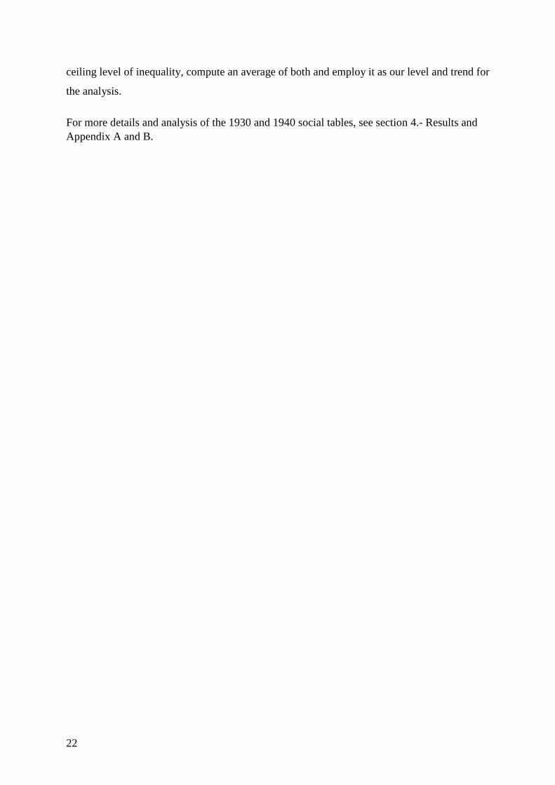
28

Occupational Group Population Share Income 1940 (1990 USD)

75

Yarns, fabrics and twists of hard

fibers workers 0.03% 1,945.62

76 Canned food industry workers 0.01% 1,926.25

77 Military 0.51% 1,921.65

78

Sweets, chocolate and syrups

workers 0.01% 1,893.95

79 Sand mining workers 0.01% 1,890.94

80 Glue industry workers 0.00% 1,868.82

81

Oils and greases for industrial use

makers 0.00% 1,868.82


83 Boudoir workers 0.09% 1,753.80

84

Sugar, alcohol and brown sugar or

brown sugar 0.09% 1741.52

85 Policemen and firefighters 0.06% 1729.48

86 Oil industry workers (refining) 0.00% 1729.06



89

Service sector employees (hotels,

restaurants) 0.07% 1492.85

90 Smiths and smelters 0.00% 1430.36

91 Peasants 10.58% 1360.72

92

Occupations not sufficiently

specified 1.86% 1325.65

93

Brooches, brushes, brooms, sieves

makers 0.00% 1298.35

94 Shoemakers 0.01% 1261.17

95 Hunters and fishers 0.05% 1106.39

96

Ejidatarios (peasants with

communal property rights) 6.21% 1096.80


98 Butchers 0.04% 872.46

99

Dough, tamales, tortillas and atole

makers 0.08% 664.22


Source: Author’s own calculation.

29

3.4 From Social Tables to the Lorenz Curves and the

Gini Index

After the construction of the social tables, what is left to do is to derive from them the income

distribution. For this purpose we employ the Mehran method, based on the work of Farhard

Mehran (1975) to obtain the Gini index based on the observed points of the Lorenz curve.

The Gini index or coefficient is a measurement (G) defined as the ratio of the mean of the

difference to two times the mean of the income distribution (Mehran, 1975). Formally it can be

stated in the following manner:

𝐺 = (1

2𝜇)∫ ∫ |𝑥 − 𝑦|𝜕𝐹(𝑥)𝜕𝐹(𝑦) (1)

Where F is the comulative income distribution function and 𝜇 is the average income. G= 1

means absolute inequality and G = 0 absolute equality.

Employing the Mehran method described in Mehran (1975), the so-called geometric method is

the best approach in our case to approximate the Gini value, because it is specially constructed

to address the problem of mean incomes that suffer from possible large margins of error as is

the case with incomes constructed from social tables.

The Lorenz curve is a graphical representation of the income distribution, it plots the

commulative income and cummulative population. The construction of the Lorenz curves allow

us to observe the changes that take place along the entire distribution giving us a deeper level

of detail that just employing the Gini index. The Lorenz curve can be formally defined in the

following manner:

𝐿(𝑦) =∫ 𝑥𝜕𝐹(𝑥)𝑦

0𝜇

⁄ (2)

Where L(y) is the cummulative distribution and 𝜇 is the mean income.

To make these computations we employ the RStudio package INEQ. For the code and the data

workflow of the calculations and the construction of the Lorenz curves consult the Appendix

C.

30

4 Results

4.1 Summary of Results

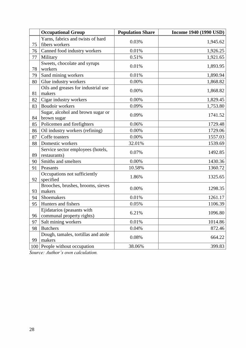
The evolution of Mexican Inequality is strikingly stable over time, especially when we compare

it to the post 1950 measurements. Inequality fluctuates around the same levels since the

beginning of the twentieth century, with only small continuous improvements over the first

decade of the twenty-first century. The only distinctive period of significant reduction being

the aftermath of the revolution, 1910-1930.

From the construction of the social tables for the four benchmark years of 1895,1910,1930 and

1940 we obtained the following Gini index values:

*As stated in Section III, we will take the average Gini as our unit for the analysis to avoid the possible

biases of the minimum and maximum level estimations.


4.2 The Evolution of Mexican Income Inequality

At the middle point of the Díaz’s government, 1895, the Gini index reached a value of 0.408, a

level that appears low compared with other Latin American societies of the time, like Chile

with a Gini index of around 0.50 (Rodríguez Weber 2014,2016). Nonetheless, it is a high level

Table 5: Mexico's inequality (Gini index) 1895,1910,1930 and 1940

1895 1910 1930 1940

Min 0.32751 0.4583 0.3112 0.4168

Max 0.48862 0.6188 0.4516 0.5259

Average* 0.40806 0.5386 0.3814 0.4713

31

if we consider that Mexico at the time was an agrarian society, with over 70 per cent of the total

population and over 50 per cent of the working population in rural areas (Estadísticas Históricas

de México, Tomo I). A large part of the population was working and living on haciendas, not

owning land and suffering strong exploitation from both government and landed elites. It

becomes relevant to ponder upon how the Mexican society reached that point?

The first half of the nineteenth century was particularly chaotic for the new Mexican republic.

After independence, the per capita GDP collapsed according to Coatsworth (1989), the

Independence War cost Mexico 4.2 points of its GDP and 21 percent in per capita terms. That

was equivalent to losing, between 1820 and 1845, 0.5 points of per capita income each year.

Other sources, like Salvucci and Salvucci (1993) point to a cost that exceeds 50 per cent of

GDP. Then, it is not hard to imagine that an economy on such a context experiences a severe

decline on well-being.

Naturally, after several conflicts, including civil wars, two prolonged foreign interventions, one

from the United States during the Mexico-American War of 1846 and the second one during

the French intervention of 1862-1867, and the War of Reform 1857-1860. After half a century

of permanent political and military conflict, the Mexican economy suffered from backwardness

and poor living standards.

After 50 years of chaos and stagnation, Benito Juárez’s government started to work on how to

transform Mexico into a capitalist industrial economy. The economy suffered from a

deteriorated road network, so in the last segment of Juárez’s government there was an effort to

channel resources towards rebuilding them, however the process was slow. The lack of money

and the turbulence of local political and military leaders and bandits prevented the further

integration of the economy.

After some failed attempts to take power, Porfirio Díaz succeeded in 1877. Díaz’s policies were

not significantly different from those attempted by his predecessors. He realised the need to

communicate the country; he started to centralise power and deployed the Rurales, a type of

militarised police created by Juárez, to combat banditry on the roads. In addition, he reformed

the “alcabalas”, a type of inner trade tariff, diminishing their effect on inner trade. These

developments signalled the possibility of a more integrated market and thus, promoted the

confidence of foreign investors. With all the foreign investment that began to arrive in the 1880s

decade, more railroads were built. The railroads integrated parts of the economy that up until

32

that moment were uncommunicated. Coatsworth (1981) estimates that freight rates fell 200 per

cent under Díaz’s government. Even though Mexico arrived late to the nascent wave of

globalisation, it rapidly adopted the new technologies of the Industrial Revolution.

Mining was one of the winner sectors of this transformation, the export of silver, similarly to

the colonial times, was one of the significant sources of revenue in the economy.

Simultaneously, this connectivity allowed the expansion of the hacienda economy to service

the mines and other industries that began to flourish. The booming economy stimulated

commerce and the creation of financial intermediaries and industries to service the sophisticated

taste for European fashion, art, and other forms of conspicuous consumption of the new

Porfirian elite.

Mexican liberal reformers had a strong sense of what the country needed to scape its

backwardness after they prevailed during the conflicts of the first half of the nineteenth century.

They saw a solution in the construction of a class of yeomen farmers (Haber, 1989) that could

propel the development of a capitalist industrial nation. The tool for this construction was blunt,

they confiscated land that belonged to the indigenous rural population.

When foreign investment began to flow through the country, it generated speculation over the

value of land. The government at the times of Juárez seised large amounts of communal land,

this policy was accelerated under Díaz. In 1883, the government passed new laws that allowed

private companies to survey land that was considered “unused” for the government. In exchange

for this surveillance, these companies could keep a third of the surveyed land, the rest would

go to the government (Haber, 1989).

Afterwards, the government could sell that land or assigned its use to productive projects. In

this way, grand extensions of land ended in the hands of a tiny minority that had enough

resources either to buy them, surveyed them or just were close enough to the government so

that the land could be assigned to them. As Markiewicz (1985) describes it, between the

Juarez’s government and 1892, 82 per cent of the rural communities, mostly of indigenous

roots, were incorporated into haciendas that found in them precious labour to be exploited.

The rural population did not welcome the expropriations and often rebelled against them.

Coatsworth (1981) explores in many details these rebellions and how the government had to

resort to brutal repression to contain them and protect the interests of the hacendados and the

foreign investors. The policy of expropriation of land, combined with the violence that expelled

33

segments of the population out of the provinces, created a flux of internal migration that arrived

to the cities looking for waged jobs in the newly created industries. In this way, the booming

economy of the time and the brutality of the Díaz’s government provided the conditions for a

proletariat class to rapidly emerge.

A structural change took place in the second half of Díaz’s government. The economy started

to expand reverting the first half of the century contraction. After 1895, the second half of the

Porfiriato, the industrialisation of the economy begun. Nonetheless, to sustain industrial

production in a national market that lacked purchasing power, the creation of monopolies was

required (Haber, 1989). Díaz’s government suffered from what is called the “commitment

problem” (Haber, 2002). The government required to attract private investment to promote

economic growth and strengthen his rule, but the state could not establish a rule of law; taxes

were often unreliable and local elites strong. To solve the commitment problem, Díaz resorted

to textbook crony capitalism, using political power to create rents that in turn provided a stable

enough compromise from both sides.

Mexican industries could not export; they were not competitive so in order to survive they

required protection from foreign competition (Haber, 1989; Beatty, 2002; Kuntz, 2002).

Another factor that contributed to the creation of a tight economic elite was the high cost of

capital. Mexican financiers often had close links with the government and used those relations

to extract rents and create networks of businessmen that controlled the significant firms around

the country. In certain ways, the Mexican financiers were the State, as government required

them to finance itself. At the same time, they controlled most industries and banks, to the point

of dictating the fiscal, monetary and commercial policies of the country (Haber, 1989).

Politically created rents stimulated an enormous concentration of income and wealth, as only a

tiny minority with access to resources and political influence controlled the value creation in

the economy. The high levels of inequality were not only a product of economic development

as theorised by Kuznets (1955), but also a result of the political economy. Businesses were

vertically integrated from the hacienda economy, where firms obtained raw resources and

materials for the factory floors. On the other hand, workers experienced some wage gains.

Nonetheless, the high rates of inflation of the last years of the Porfiriato vanished them. Hence,

in 1910, the year the Mexican Revolution begun, our social tables register a Gini index of 0.538

on average, with a maximum possible level of 0.618. Either value represents the highest Gini

index recorded in Mexican economic history.

34

Figure 1 displays something similar to the Ravallion and Chen (2003) and the Milanovic and

Lekner (2013) growth incidence curves. These “growth incidence bars” show the income gains

that each occupational group had between 1895 and 1910 according to our social tables.

Hacendados, the merchant financiers and the top echelons of government were the clear winners

and the workers and peasants the clear losers.

When looking at the reconstruction of the rate of returns done by Haber (1989), for some of the

leading firms during the 1902-1910 period, we find a rate of return that moves around 7 per

cent for most years and from 1896-1910, yields on stocks that average 5 per cent. This finding

is in line with Piketty’s hypothesis of r>g (Piketty, 2014) as GDP per capita growth was on

average 2.1 per cent (Bolt et al. 2018, The Maddison Project Database).

Piketty’s hypothesis, that if the rate of returns exceeds economic growth the capital holders, in

our story the Mexican merchant-financiers and large landholders, will accumulate resources at

a faster rate than the rest of the economy, appears to be vindicated.

Recently published evidence from Jordà, Knoll, Kuvshinov, Schularick, and Taylor

(Forthcoming) shows that except for World War II, r>g has been the norm for the last 150 years.

For the Mexican case, it is a suitable candidate for explaining the leap in inequality levels that

we observe in the 1895 and 1910 social tables.

Source: Author's own calculation.

Figure 1: Winners and losers: real gains by occupational group 1895-1910

35

While rents were high, working conditions for the agrarian population were harsh and wages

were low. The German agronomist Karl Kaerger (1902), in a research mission from the German

Kaiser, surveyed the possibility to substitute imports from the United States agriculture for

Latin American ones in case of war. Kaerger arrived to Mexico to observe agricultural

production and labour conditions. In his report, Kaerger describes the low wages paid to

Mexican peasants and how these labour conditions, low labour costs and possible high profits

in agricultural exports, were favourable for German investments. Wages were so low that The

Mexican Economist (El Economista Mexicano, May 7, 1904) a weekly newspaper dedicated to

economics and finance at the time, reported that the rural population, in a bad harvest year,

were unable to afford clothing.

Díaz’s government saw itself in the positivist tradition of Auguste Comte. His cabinet members

were even called the “scientists” due to their idea of ruling employing scientific management

and unregulated market economy policies. Often this policy was not as pure as they presumed.

In an open economy, rapidly integrating to the global markets some distributive effects are

expected. The Stolper-Samuelson theorem (Stolper & Samuelson, 1941) and the Heckscher-

Ohlin model (Hecksher, 1931) would predict that the intensive factor of production in a country

like Mexico, unskilled labour, would be utilised with more intensity and would gain from trade.

Meanwhile, the less intensive factors, skilled labour and capital would lose. That is not what

occurred in Mexico. Government protection of industries prevented this type of distributional

forces. Besides, the Porfirian regime had as a core principle the freezing of the existing

distribution of resources and political power. For that reason, the government actively resisted

the creation of an organised working class. Any attempt to demand higher wages or improve

the labour conditions was ignored, any attempt of a strike in a factory was met with force.

The Lorenz curves for 1895 and 1910, Figures 2 to 4, reveal the nature of some of these changes,

the winners and losers of the liberal modernisation project of the Díaz’s government. From

1895 to 1910, we observe how the distribution skews towards the upper side of the income

distribution. Even if the overall population appears to have experienced some income growth,

it is disproportional in favour of a few groups, like the top government bureaucracy, the

industrialist’s merchant-financiers and the large landowners.

36

Figure 2: Mexico's Lorenz curves 1895 & 1910 min max levels


Figure 3: Mexico's Lorenz curves 1895 min max levels.


37



We know from historiographic sources that the large concentration of economic power and the

exploitation behind it created conditions favourable for the peasants and proletariat to revolt.

At the end of the Porfiriato, revolts ended in a massacre, like the Rio Blanco revolt of 1907

(Gómez-Galvarriato, 2002). Additionally, the close relationship between the concentration of

wealth and income and political power became a barrier for local elites, particularly in the North

of the country. The political economy of the Díaz’s regime, with its success in creating growth

that benefited a small clique of cronies, created the conditions suitable for its demise.

The Mexican Revolution overthrew Díaz’s regime, but it did not have a unified ideological

agenda or goals (Gómez-Galvarriato, 2002). The labour movement hard earned the changes in

labour relations that took place from 1911 and onwards. In 1911 the first general strike was

successfully conducted in the textile industry in the states of Veracruz and Puebla, leading to a

collective contract and the unionisation of the textile industry (Bortz, 2002). The gains for the

popular classes did not arrive from the revolutionary political agenda that to some extent

represented the interest of some of the neglected economic elite and petite bourgeoisie. It was

an accident, a by-product of the revolutionary process itself.

38

The bloodiest years of the revolution took place after the assassination of president Madero in

the beginning of 1913. The period started with the overthrow of Madero’s usurper, Victoriano

Huerta and then faction infighting commenced among revolutionary groups. This part of the

Mexican Revolution closely behaves like a civil war, governments lasted for short periods and

therefore were weak. This weakness made local and national governments make enormous

concessions to workers at a scale not hitherto dreamt of. For example, as documented by Bortz

(2002), some state governors like Luis F. Domínguez from Tabasco and Candido Aguilar from

Veracruz decreed minimum wage increases, regulated the maximum working hours per day,

abolished debts and prohibited physical punishment at factories. This development most likely

had an impact on income inequality.

Considering its importance, the second decade of the twentieth century is a period surprisingly

neglected in the Mexican economic historiography; this because of the lack of reliable sources

of data. The population census of 1920 does not allow us to construct a social table to proxy for

the income distribution and other sources are not available, for example, statistical yearbooks

or economic censuses. Nonetheless, it is reasonable to assume that inequality decreased.

Mexican economic elites lacked ideological cohesion during the Revolution, therefore were

unable to protect their interests as before. On the other hand, the popular classes began to

conquer economic and political rights. This shift in political power can be illustrated by the

Venustiano Carranza’s series of decrees from the beginning of 1915 which restored lost land to

peasants, extended the new labour law to all the country and increased the minimum wage.

At the height of the faction infighting of the Mexican Revolution, peasants and workers became

a vital source of men for the revolutionary armies. In 1915 Carranza’s Constitutionalist Army

(Ejercito Constitucionalista) engaged in a ferocious war with Francisco Villa’s Northern

Division (La División del Norte) and at a lesser extent with Emiliano Zapata’s army, the latter,

although less of a military threat, provided the ideology for the revolution. Thus, Carranza’s

concessions to the working classes that fielded his army were a necessity. The 1917

Constitution’s recognised labour and social rights, yet it was resisted by the economic elite and

Carranza himself, therefore it was a conquest of the popular classes that now had a seat at the

political table (Bortz, 2002). The claim that the Mexican Revolution decreased inequality can

be supported by the number of successful strikes since 1920.

39

Table 6: Strikes and resolutions 1920-1936

Year Strikes Workers Favour

workers

Favour

owners

Negotiated Not

known

1920 173 88,536 30.00% 30.00% 40.00% 0.00%

1921 310 100,380 13.23% 13.23% 61.29% 12.26%

1922 197 71,382 45.69% 45.69% 8.63% 0.00%

1923 146 61,382 28.77% 28.77% 42.47% 0.00%

1924 136 23,988 50.74% 23.53% 25.74% 0.00%

1925 51 9,861 50.98% 15.69% 33.33% 0.00%

1926 23 2,977 34.78% 34.78% 13.04% 17.39%

1927 16 1,003 25.00% 25.00% 50.00% 0.00%

1928 7 498 71.43% 14.29% 14.29% 0.00%

1929 14 3,473 42.86% 35.71% 14.29% 7.14%

1930 15 3,718 80.00% 13.33% 6.67% 0.00%

1931 11 227 72.73% 0.00% 0.00% 27.27%

1932 56 3,574 10.71% 26.79% 53.57% 8.93%

1933 13 1,084 61.54% 15.38% 0.00% 23.08%

1934 202 14,685 47.52% 52.48% 0.00% 0.00%

1935 642 145,212 45.48% 16.36% 31.31% 6.85%

1936 674 113,885 75.82% 12.46% 5.04% 6.68%

Source: Mexico’s Statistical Yearbook 1935.

From the year 1920 up to 1936 strikes intensified and most of the time favoured the workers or

required a negotiated solution in which both workers and owners had to make concessions. This

state of affairs was unthinkable before the revolution and lead to significant improvements in

the working conditions and wage increments. It has long been recognised in the inequality

literature that rising minimum wages have a strong influence in inequality levels (Autor,

Manning and Smith, 2016).

Also, the construction of the 1930 social table provides us with an estimate for inequality levels

after the Mexican Revolution ended. Inequality in this year is at its lowest point in more than a

century with an average Gini index of 0.381 and a possible minimum of 0.311. The Mexican

revolution arguably ended in 1921, after most revolutionary leaders were dead and a faction

claimed victory, however, soon after this conflict ended a minor religious war erupted, ending

in 1929.

We know from the social tables that inequality was at its highest point in 1910 and we know

that the mechanisms that produced that high concentration of income were land grabbing and

40

the creation of rents. We also know that inequality in 1930 was at its lowest point. What

mechanisms account for this evolution?

One mechanism must be the revolutionary violence, Scheidel (2017) argues that war and

destruction are a source of levelling, and even explicitly mentions the Mexican Revolution and

its agrarian reform as an example (Scheidel, 2017 p. 347). However historiographic evidence

suggests that the destruction of capital was not generalised (Womack, 1978; Haber, 1989).

Revolutionary armies captured factories and haciendas and exploited them to obtain resources

to sustain their military operations. Haber (1989) describes how the economic elite was left

untouched after the revolution and shows how industrial output recovered after the fighting

stopped. Owners even managed to retain political power, for example, influencing the draft of

the 1917 Constitution (Bortz, 2002). Katz (1974, 1998) describes how after the revolution some

of the confiscated lands were returned to their previous hacendado owners.

These facts imply that the destruction of capital channel of Scheidel was not the driver of the

levelling process. Nonetheless, violence did play a role in the levelling, as it provided the

popular classes with some bargaining power to wrest concessions out of the elites. The Mexican

Revolution impacted inequality in more subtle ways, like labour rights, social rights, education

and health services, the introduction of income taxation and large-scale land reform, and

through the institutional reforms of the 1917 Constitution.

The income tax was first introduced in 1924, even if it was a very low rate it slightly compressed

the income distribution. The same can be argued about the inheritance tax introduced in 1926.

Labour rights can be illustrated with the number of strikes that resulted in favour of the workers.

For example, according to Gómez-Galvarriato (2002), from 1920 to 1929 real wages increased

131 per cent, with some regional variations due to the differences in the strength of the labour

movement. Perhaps the more significant source of redistribution came from the land reform,

which created new owners that could derive income from the land. Even if the economy was

about to experience a modern take-off, during the decade of the 1920s the agricultural sector

still contributed the highest share to national income.

From 1895 to 1930 it is clearly distinguishable how the political economy created winners and

losers. The political decisions to either create rents or redistribute land and increase wages

impacted the income distribution. It was not a Kuznetsian evolution of the economy that created

inequality as a process of economic development; it was a series of political choices.

41

In the 1930 to 1940 decade, the story is slightly different; we observe an increase of inequality

in a period in which social rights and public services expanded; also, social policy had a strong

influence on well-being. This increase shares some common mechanisms with the previous

evolution, but for this period it is closely related to the Kuznests hypothesis as industrialisation

took off with the Second World War.

The Gini index obtained for 1940 from the social table was 0.471, a level above the 1895

average level and close to the possible maximum registered in 1895. During the decade between

1930 and 1940 social policy and land redistribution augmented, particularly during the Lazaro

Cárdenas’ government 1934-1940. Cárdenas’ policies accelerated the land reform

redistribution and promoted extensive national campaigns to train professors and medics and

then deploy them around the country.

During the same period, as the recovery from the Great Depression took place and the hostilities

of the Second World War started, the Mexican industrial sector experienced fast growth rates.

Large infrastructure projects stimulated demand for industrial goods and Cárdenas strongly

favoured investments in social housing for workers (Davis, 1994). In one hand we have the

equalising forces of social policy and land redistribution and in the other the Kuznetsian

increase in inequality due to rapid economic development.

Cárdenas’ government maintained some tensions with Mexican industrialists. During his

government, their influence on policy was reduced, and the popular classes increased their

political participation. Alan Knight (1991) sees the acceleration of the land redistribution under

Cárdenas as favourable to the well-being of the peasants and as a source of change in the

political equilibrium.

However, even if Cárdenas’ government managed to successfully negotiate with all political

sectors, including the newly enfranchised peasantry and produce a better distribution of the

gains of growth, it does not mean that it totally broke the cronyism that allowed for the political

creation of rents. Haber, Rozo and Maurer (2003) call this phenomenon “vertical political

integration” and it can be seen as an element of the monopolistic nature of many industries

since the end of the nineteenth century to the first decades of the twentieth-first.

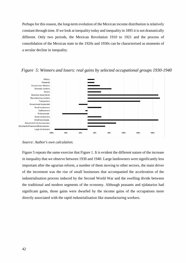
42

Perhaps for this reason, the long-term evolution of the Mexican income distribution is relatively

constant through time. If we look at inequality today and inequality in 1895 it is not dramatically

different. Only two periods, the Mexican Revolution 1910 to 1921 and the process of

consolidation of the Mexican state in the 1920s and 1930s can be characterised as moments of

a secular decline in inequality.


Figure 5 repeats the same exercise that Figure 1. It is evident the different nature of the increase

in inequality that we observe between 1930 and 1940. Large landowners were significantly less

important after the agrarian reform, a number of them moving to other sectors, the main driver

of the increment was the rise of small businesses that accompanied the acceleration of the

industrialisation process induced by the Second World War and the swelling divide between

the traditional and modern segments of the economy. Although peasants and ejidatarios had

significant gains, those gains were dwarfed by the income gains of the occupations more

directly associated with the rapid industrialisation like manufacturing workers.

Figure 5: Winners and losers: real gains by selected occupational groups 1930-1940

43

Figure 6: Mexico's Lorenz curves 1930 & 1940 min max levels.




44



Table 7: Incomes and ratios between occupational groups, Mexican pesos 1895 1910 1930 1940

workers wage* 382.50 460.00 861.43 1678.82

peasants wage 171.76 272.48 496.40 708.10

businessmen income 14,208.71 27,119.15 25,653.40 44,236.84

Large landowners

income

105,403.50 249,183.22 51,560.04 16,816.67

Ratio workers/peasants 2.23 1.69 1.74 2.37

Ratio

businessmen/workers

37.15 58.95 29.78 26.35

Ratio

businessmen/peasants

82.72 99.53 51.68 62.47

Ratio Large

Landowners/workers

275.56 541.70 59.85 10.02

Ratio Large

Landowners/peasants

613.67 914.50 103.87 23.75

Ratio Large

Landowners/businessmen

7.42 9.19 2.01 0.38

*For 1930 and 1940 the workers wage is the average of industrial occupations.

Source: Author’s own calculations

45

From 1930 and 1940 Lorenz curves Figures 6, 7 and 8 and Table 7, we can distinguish how

inequality was not only driven by the top income gains, but from differences between skilled

workers around the middle of the distribution and unskilled workers at the bottom of it. The

1930 distribution is significantly compressed as it can be seen in the decline of the ratio of

landowners' income to other benchmark classes. In 1940 the fast industrialisation of the

economy favoured skilled urban workers over the still numerous rural population, as can be

seen in the recovery of the ratio of workers’ income to peasants’ income. At the same time, we

observe how land stops being the primary source of income, the large landowners' ratio to

workers dramatically diminishes, and the businessman ratio to other classes becomes the larger

one. All these evidence points to a Kuznetsian process taking place in that decade.

Nevertheless, the fact that land stopped being the primary source of income does not necessarily

mean the old elites disappeared. As Wasserman (1987) points out, the old elite employed

several strategies to survive; for example, dividing their lands to avoid the land reform, selling

them to foreign investors, diversifying their investments and marrying members of the new

regime. In this sense, the capacity of the old economic elite to survive and retain some degree

of economic influence is reminiscent of the recent findings of Ager, Platt Boustan and Eriksson

(2019) in the postbellum United States and the economic recovery of former slave-owning

families. These mechanisms could be part of the explanation behind the rise in inequality

between 1930 and 1940.

Another important aspect to keep in mind is the female participation in the economy. Female

participation before the Mexican Revolution was concentrated in occupations such as domestic

work and servitude with very low wages.

After the revolution this changed, during the 1930s and the government of Lazaro Cárdenas

women were able to participate on a broader set of occupations and enjoy some of the benefits

of education. However, gender inequality most likely persisted. An illustration of this comes

from the writings of the Mexican diplomat, novelist and poet Rosario Castellanos in her novel

Balún Canán, where she describes the class conflict between the rural population and especially

indigenous women trying to materialise the gains from the Cárdenas’ reforms against the

resistance from the economic elites. At the end, even if the Cárdenas’ government implemented

reforms, redistributed land, enfranchised people and promoted social services, the huge

disparities among the haves and the have-nots eventually resumed.

46

4.3 History is the rock upon which economic theories

survive or are broken

History is the true test for economic theories, in light of our results, what can be said about the

dominant theories of the evolution of inequality in the Mexican context?

First, the Kuznets hypothesis, we indeed observe to some degree the characteristical increase

in inequality as industrialisation accelerates; however, it cannot explain by itself the evolution

we see. Over the whole period of 1895 to 1940 we can only claim the existence of something

like the Kuznetsian process from 1930 to 1940. The increases from 1895 to 1910 and the

decrease we observed from 1910 to 1930 do not match with this traditional explanation.

Mexico was a predominantly agrarian society with most of its population living in rural areas

and working on the traditional sectors of the economy, like small-scale agriculture up until the

1960s. The Kuznets hypothesis works bests for countries facing rapid urbanisation (Lindert &

Williamson, 2016), but at the time, that was not the case for Mexico. For the Mexican scenario,

the distribution of the land appears to be the main factor behind distributional changes; this is

something commonly neglected in inequality studies and particularly relevant in historical

contexts as demonstrated by Lindert and Williamson (2016) for incomes in the United States

and by Bengtsson, Missiaia, Olsson and Svensson (2018) for wealth in Sweden.

Second, the institutionalist point of view is very relevant in this case. However, it is not in the

same way as thought by Engerman and Sokoloff (1997, 2012) or Acemoglu, Robinson and

Johnson (2001, 2002). Extractive institutions did play a prominent role, the vertical political

integration allowed for cronyism and rent-seeking behaviour, however, it was not a product of

inherited institutions, but a consequence of the political economy circumstances of the time. To

survive the Mexican governments of the period had to make allies with those who could provide

them resources and then after the revolution by a corporatist arrangement.

The ECLAC structuralist school, represented in the works of Cardoso and Falleto (1967) and

Pinto (1973), is concerned with the problem of structural heterogeneity, that is, the existence of

several stages of development at the same time in the same country, which is closer to the Latin-

American reality than the more orthodox institutionalist approach. Haber’s (2002) commitment

problem is also useful for understanding how institutions had an impact on the distribution of

income as governments tied themselves to private interests to sustain their power.

47

Third, the Williamson (2010, 2015) and Dobado (2010) hypothesis that argues in favour of the

nineteenth century commodity boom as the source of inequality in Latin America does not

match the Mexican circumstances. The Mexican industrialists did try to take advantage of the

first wave of globalisation. They tried to export both commodities and manufactures but were

not very successful. They were not competitive and they lacked a strong inner market to sell

their production, requiring significant amounts of protection. The government ended up carving

monopolies and oligopolies for them. The first globalisation cannot be the primary driver of

inequality between 1895 and 1910; clearerly politically created rents that skewed the

distribution of income are a more apparent culprit.

Fourth, Piketty’s r>g and the changes due to taxation and the welfare state related policies

partially apply in the Mexican context of 1895 to 1940. The rate of return of capital for the

period, did exceed the rate of economic growth. The owners of capital, the large landowners’

and industrialists’ incomes greatly surpassed the popular classes as can be seen in Table 7. We

also know from the literature that after the Mexican Revolution several conquests were made

by the popular classes, labour rights, healthcare services and education; income and inheritance

taxes were created, so after the 1930s redistribution intensified. Thus, the Pikketian mechanism

fits some of the developments and cannot be easily discarded, the rate of return matches, but

taxes had a marginal impact.

Finally, the destruction mechanism claimed by Scheidel (2017) becomes relevant. As we have

argued before, the Mexican Revolution did not destroy large amounts of capital, it left the

economic elite largely untouched; hence, destruction of capital cannot be the source of levelling

between 1910 and 1930. However, similarly to the institutionalist view, the revolution was

indeed a source of levelling but in a subtle manner. It was the recognition of the peasantry and

proletariat as legitimate political actors that wrestled concessions from the elites. Moreover, it

was the recognition of social rights and the need to pacify the country that turned out to be the

great leveler.

Therefore, the Scheidel (2017) argument of revolution as a source of levelling might need to be

thought in a more complex manner, the type of revolution matters for the levelling process.

Taking into consideration Barrington Moore’s (1966) three types of revolutions: agrarian

revolutions, bourgeoisie revolutions and aristocratic revolutions, one can see that the Scheidel

mechanism is present in the agrarian type of revolution, for example in China and Russia.

Nonetheless, the Mexican Revolution shares characteristics with the agrarian and the

48

bourgeoisie types. Therefore, we can observe opposing mechanisms at play, an agrarian reform

and a set of social rights that promote equality and the survival of segments of the economic

elite and the defense of bourgeoisie interests pulling in the opposite direction.

Following these findings, the land ownership dynamics become even more relevant, as pointed

by Lindert and Williamson (2016), in countries with sharp differences between rural and urban

sectors, inequality is shaped by often opposing forces. The rural population becoming more

equal relative to themselves in terms of income, but more unequal relative to urban populations

where industrial jobs and human capital-intensive jobs can obtain more income. Between 1930

and 1940 we observe different forces oppose each other, the occupations centred in rural areas

stagnated and fell behind, on the other hand, urban occupations, associated with the

industrialisation and urbanisation process, like small business and industrial workers, were able

to earn higher wages and salaries.

What we can see then is that no single theory about inequality is a perfect fit, the evolution of

inequality in Mexico between 1895 and 1940 is a multifactorial process. If we take a long-term

perspective and observe not only the period of our study, but the evolution up to the present

time, the necessity for a more contextual explanation is even more evident, but this discussion

is better suited for our concluding remarks.

49

5 Conclusions and Further Discussion

5.1 Inequality as a Political Choice

Thinking about the the 1895-1940 period, it becomes difficult not to consider the Mexican

Revolution as more Bonapartist, in the Marxist use of the term (Marx, 2015 [1852]), than

radical, as the faction that prevailed at the end of the conflict represented the interests of the

bourgeoisie and the surviving Porfirian economic elite. Therefore, this faction only made

concessions to the proletariat and rural classes out of political necessity. Gilly (1971)

characterises the Mexican Revolution as an economic elite fighting with its rival factions for

political power and access to rents, peasants that wanted to restore the status quo to the pre-

capitalist economy and stop exploitation and workers that wanted a post-capitalist arrangement

with social, economic and political rights. Since the economic elite that eventually won did not

have an ideological cohesion, instead adopted a pragmatic approach to power during the

conflict; all the conquests of workers and peasants that ended in the Mexican Constitution of

1917 were a compromise. Nonetheless, although this was a dramatic improvement that freed

capital and labour to be employed in more efficient ways (Womack, 2012), it did not entirely

extinguish the political economy of the Mexican ancien régime, it merely included fractions of

new groups in it.

In a simile to the French Revolution, the Mexican one also had its Thermidorian Reaction. It

temporarily changed the inequality dynamic as the country required peace. Governments, either

by the understanding of that peace as a requirement for economic development or because of

merely sympathy for the popular classes, mustered the political will to enact policies that

reduced inequality. The Mexican Revolution eventually faced its Thermidor by leaving the

vertical political integration alive. This cronyism would be one of the mechanisms that

prevented inequality to further decrease over the twentieth century and turned into a source of

many of the economic problems the country has faced up to this day.

For example, Tocqueville (2006[1856]) in his book The Old Regime and Revolution, and Marx

(2015[1852]) in his Eighteenth Brumaire of Louis Bonaparte concluded, when examining the

50

French Revolution, bourgeoisie or Bonapartist revolutions change the economic and political

elites, but not the political structures. The Mexican Revolution in the fragile equilibrium it

wanted to preserve between all social classes, ended embracing a corporativist structure that

although more inclusive than before, still maintained some of the old structure of power.

As Bleynat, Challú and Segal (2017) point out, inequality in Mexico does not seem to follow

the Kuznets process, the changes in inequality are more intertwined with the political sphere

and the policies implemented by the ruling classes than to economic development alone.

Milanovic and Bustillo (2008) argue that in Latin America the Kuznets hypothesis does not

hold. Inequality appears to be rather persistent over time regardless of the development level.

When looking at the long-term evolution for the Mexican case in Figure 9, that statement is

confirmed. In Mexico, income inequality has remained high for more than a century, even after

intense periods of economic growth. The Kuznets hypothesis states that inequality should rise

after the initial states of economic development and then decrease after a certain level has been

attained. Nonetheless, development and inequality in the Mexican case have followed each

other hand in hand for as long as we can measure. In the most optimistic reading of the data,

we could claim the existence of tenuous Kuznets wave (Milanovic, 2016) but on the worst,

inequality has almost remained the same.

Source: For 1895,1910, 1930 and 1940 author’s own calculations. For 1950-2004 Székely

(2005). For 2008-2016 Coneval.

Figure 9: The evolution of inequality in Mexico: 1895-2016

51

This persistence challenges prevailing theories of how inequality behaves. In the past, referring

to our 1895 and 1910 estimates, the property of land is the main factor behind inequality

changes, owning land meant having a production to sustain oneself and a surplus to sell to the

market. Owning land meant controlling natural resources that were key for new industries, it

meant having collateral resources to access the tight financial market of the time. Not owning

land meant being dispossessed and with little choice but to sell your work to the landed elite or

migrate to the cities seeking employment in the nascent industrial sector. Few people had

freedom due to lack of entitlements and this is especially true for women and the indigenous

population as their work were concentrated among the occupational categories with lower

wages.

Historically, the Kuznets hypothesis and the new institutionalist view were held as the primary

explanations behind inequality; nonetheless, over the years historical evidence for developed

and developing countries alike do not support the Kuznets hypothesis validity anymore and the

institutional view is debatable according to each country’s history. Developing countries have

heterogeneous economies arriving late to the industrial revolution, failing to integrate rapidly

to the global economy and with different geographies, colonial histories and most importantly

their own historical contexts; hence developing countries require a tailor-made analysis that

often general theories omit for simplicity.

At the end of the nineteenth century, Mexico was not a pure capitalist economy; even to this

day, the country faces dualism with powerful and dynamic technologically advanced modern

economic sectors and weak and stagnated traditional ones still employing nineteenth century

techniques. Developing countries, particularly Latin American countries, can be thought as

different countries living inside the same geographic boundaries. For that reason, detailed

contextual analyses are required to understand how inequality changes.

If the concept of structural heterogeneity is valid, and there are reasons to think it might be,

then inequality in developing countries needs to be thought in a way that addresses this specific

set of circumstances. If as Pinto (1973) argues, Latin American countries have within sector

differences in technologies and institutions in which development does not occur at the same

pace, then inequality ought to follow different patterns. If large sectors of the economy are

consistently not capitalist yet inhabit or even overlap with more modern and capitalist ones, it

is straightforward to see why standard theories fail to explain the evolution of inequality.

52

From our findings, it comes to be clear that land ownership played a critical role in the dynamics

of the distribution of income. In the contemporary and historical context, this role seems to be

often underestimated or even entirely ignored. One hundred years ago or even today developing

countries still have large rural populations, subsistence agriculture and are reliant on light

industries and commodity exports. Therefore, the ownership of land and the share of population

in the rural sector in such countries can play a significant role in explaining inequality today. If

inequality reduction is in the global political agenda for social justice motives and economic

development, this often-ignored mechanism needs to be taken more seriously in present debates

about structural change and its distributional consequences. The Mexican experience of 1895

to 1940 serves as an excellent example of what type of policies can compress the income

distribution and what political economy challenges could arise from it.

In the present work we set to answer the following questions:

a) What was the level of inequality from the late Porfiriato to post-revolutionary Mexico,

1895-1940?

b) Can Inequality be explained by structural change forces alone? Alternatively, could it be

the result of the political-economy process?

c) Did the Mexican Revolution produce a change in the levels of inequality? Moreover,

through which channels did they change?

d) Did the agrarian reform lead to higher incomes among the agrarian population and thus

had an impact in the inequality levels?

e) Did the introduction of labour and social rights lead to higher wages and thus had influence

in the inequality levels?

Thus, we successfully answered them. Regarding question a) and b) we found that the Gini

index for the four benchmark years were: 0.40806 in 1895, 0.5386 in 1910, 0.3814 in 1930 and

0.4713 in 1940. Increasing and then decreasing to rise again. In the long-term view, Figure 9,

we can see that the levels that our social tables capture are not much different from current

levels. Therefore, we find that the structural change, the Kuznets hypothesis by itself is not

enough to explain the evolution of inequality. Only between 1930 and 1940 we can distinguish

with clarity the Kuznetsian forces at play. With confidence, we can claim that the political

economy process played a crucial role.

53

For questions c), d) and e) we find that indeed the Mexican Revolution played a pivotal role in

the decrease of inequality that followed the start of the conflict up until 1930. The Mexican

Revolution produced a series of institutional changes through the Mexican Constitution of 1917

that compressed the income distribution. The introduction of labour rights, social rights and the

welfare policies that were implemented were a direct result of the political power gained by the

popular classes. As a product of the Mexican Revolution, the agrarian reform had an impact on

rising income among the peasantry and the new class of ejidatarios, though at the moment the

new industrial sectors were increasingly important and the traditional sectors were losing

ground. The social tables of 1930 and 1940 and Figures 5 to 8 distinctly show their gains.

Finally, the introduction of social and labour rights also reduced inequality, Table 6 illustrates

how workers with labour rights could organise strikes and conquer benefits.

In answering those questions, this thesis makes distinctive contributions. First, it provides the

first empirical account of Mexican inequality levels before 1950. The measurements from the

1895 to 1940 period are the first income inequality estimations produced for that time. Second,

it offers a discussion about the adequacy of the most prominent theories of inequality and its

suitability to the Mexican case. In doing so, it makes a case for the importance the ownership

of land has in explaining inequality dynamics in historical contexts and for developing countries

with large agrarian populations. Third, the findings deliver valuable lessons for fighting

inequality today, not only in Mexico but in other developing countries, the main one being that

inequality is often politically constructed, the result of the policy decisions and the interplay

between those who hold political and economic power. The traditional view of inequality as a

secondary effect of the development process is not always true. If inequality is the result of the

existent political economy, it can be reduced through political action.

5.2 Persistent Inequality?

As a further point of discussion and a possible extension of the present work is the remarkable

persistence of inequality over the long run in the Mexican economy. Historical inequality

studies have suggested different patterns or behaviours, for example, the Kuznets waves or

cycles and the standard Kuznets hypothesis. Kuznets waves have been documented for several

countries dating back to even centuries for countries like Spain (Alvarez del Nogal & Prados

de la Escosura, 2013), Chile (Rodriguez Weber, 2014), England and the United States

54

(Milanovic, 2016). Over time, this evidence shows large swings often linked to changes in land

ownership and structural changes in the economy. However, cases like Mexico, reported here,

are not common. Mexico displays very small variations over the long run, if we discount the

hard swings produced by the Mexican Revolution and compare the trend with the post 1950

development, inequality is stable and when it is reduced, the contraction is slow and small, even

in the presence of strong and time consistent land redistribution and fast industrialisation.

Against the existence of persistent levels of income inequality, it could be argued that although

the Gini index displays similar values through time, the country indeed has changed and today

is richer than the period of study for this work. Labour exploitation is not at the same levels as

in the end of the nineteenth century or the beginning of the twentieth century. Nonetheless, a

counterargument could be made by pointing out that Mexico remains a highly unequal country

and the sources of inequality are at the core, still connected to access to public services, lack of

the facto labour rights, severe regional differences and the political process that allows the state

to be captured by private interests.

As pointed in our observation of inequality as a political phenomenon, if we draw upon the

most optimistic view, maybe taking a long term perspective, we can consider changes produced

by the revolution as a Kuznets wave. Nonetheless, unlike other Kuznets waves that can be

observed over centuries, in Mexico inequality reverses fast to the previous levels. This fast

reversal points to the contingent character of the evolution of inequality in the described

political context and the radical changes that occurred in a short period of time.

If we strictly focus on the long-term evolution of this trend, and we zoom out from the

revolutionary changes we chose to focus on this work, then we still need to explain why a quasi-

constant inequality level is possible? Redistribution or the lack of it cannot fully explain this

evolution.

From this reality two possible extensions are required. First, it is necessary to look further back

in time to the middle of the nineteenth century or even further back to its beginning. Maybe in

a larger time horizon the apparent persistence becomes an illusion. If on the other hand the

persistence is real, the second possible extension can come from the study of the so-called

structural heterogeneity of the economy, the very different development paths that exist inside

the productive sectors and the effect it has on the distribution of resources.

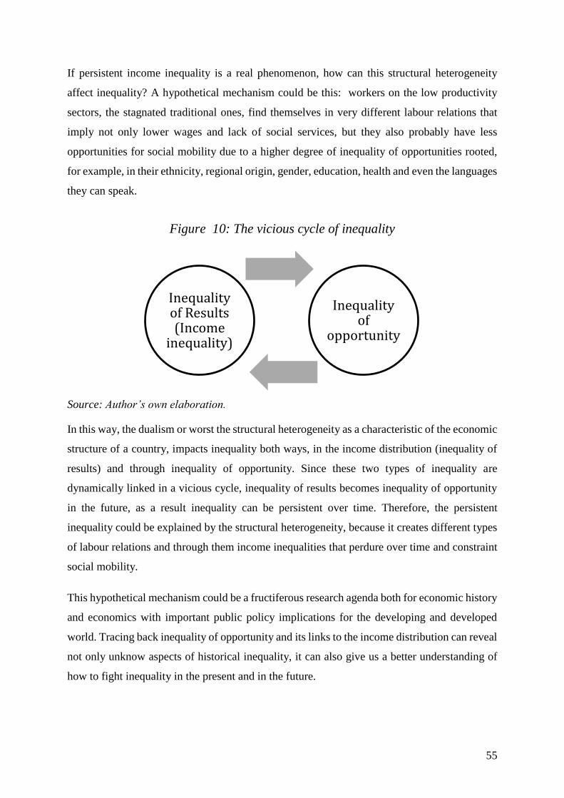
55

If persistent income inequality is a real phenomenon, how can this structural heterogeneity

affect inequality? A hypothetical mechanism could be this: workers on the low productivity

sectors, the stagnated traditional ones, find themselves in very different labour relations that

imply not only lower wages and lack of social services, but they also probably have less

opportunities for social mobility due to a higher degree of inequality of opportunities rooted,

for example, in their ethnicity, regional origin, gender, education, health and even the languages

they can speak.

Figure 10: The vicious cycle of inequality

Source: Author’s own elaboration.

In this way, the dualism or worst the structural heterogeneity as a characteristic of the economic

structure of a country, impacts inequality both ways, in the income distribution (inequality of

results) and through inequality of opportunity. Since these two types of inequality are

dynamically linked in a vicious cycle, inequality of results becomes inequality of opportunity

in the future, as a result inequality can be persistent over time. Therefore, the persistent

inequality could be explained by the structural heterogeneity, because it creates different types

of labour relations and through them income inequalities that perdure over time and constraint

social mobility.

This hypothetical mechanism could be a fructiferous research agenda both for economic history

and economics with important public policy implications for the developing and developed

world. Tracing back inequality of opportunity and its links to the income distribution can reveal

not only unknow aspects of historical inequality, it can also give us a better understanding of

how to fight inequality in the present and in the future.

Inequality of Results (Income

inequality)

Inequality of

opportunity

56

References

Archival and Statistical Sources

Departamento de la Estadística Nacional (1932). Anuario de 1930. Talleres Gráficos de la

Oficina de Agricultura y Fomento. D.F: México.

Dirección General de Estadística. (1894). Anuario Estadístico de la República Mexicana 1893.

Oficina de la Secretaria de Fomento.

Dirección General de Estadística. (1895). Anuario Estadístico de la República Mexicana 1894.

Oficina de la Secretaria de Fomento.

Dirección General de Estadística. Censo General de la República Mexicana 1895. Available

Online: http://www.beta.inegi.org.mx/programas/ccpv/1895/ [Accessed 24 November 2018]




Online: http://www.beta.inegi.org.mx/programas/ccpv/1910/default.html [Accessed 24

November 2018]




Online: http://www.beta.inegi.org.mx/programas/ccpv/1910/default.html [Accessed 24

November 2018]



Dirección General de Estadística y Departamento de los Censos. (1959). Censos Agropecuarios

1930,1940 y 1950. Talleres Gráficos de la Nación, D.F: México.

57

Dirección General de Estadística. (1949). Segundo Censo Ejidal de los Estados Unidos

Mexicanos 1940: Resumen General. Talleres Gráficos de la Nación, D.F: México.

Dirección General de Estadística. (1930). Primer Censo Agrícola Ganadero 1930. Talleres

Gráficos de la Nación, D.F: México.

Dirección General de Estadística. (1937). Primer Censo Ejidal 1935: Resumen General.

Departamento Autónomo de Prensa y Publicidad, D.F: México.

Dirección General de Estadística. (1933). Primer Censo Industrial de 1930. Departamento

Autónomo de Prensa y Publicidad, D.F: México.

Dirección General de Estadística. (1939). Anuario Estadístico de los Estados Unidos Mexicanos

1938. Departamento Autónomo de Prensa y Publicidad, D.F: México.

Dirección General de Estadística. (1943). Tercer Censo Industrial de los Estados Unidos

Mexicanos 1940. Talleres Gráficos de la Nación, D.F: México.


1941. Talleres Gráficos de la Nación, D.F: México.


1946. Talleres Gráficos de la Nación, D.F: México.

Dirección General de Estadística. (1956). Estadísticas Sociales del Porfiriato 1877-1910.

Talleres Gráficos de la Nación, D.F: México.

El Economista Mexicano. 7 of May 1904. P 114. Mexico City.

Escuela de Ingenieros de Guadalajara. (1902). Apuntes sobre instrucción en Jalisco. Boletín de

la Escuela de Ingenieros de Guadalajara, January, 1902, No 1. Hemeroteca Nacional de México.

Instituto Nacional de Geografía y Estadística. Archivo Histórico. Available Online:

http://www.beta.inegi.org.mx/app/archivohistorico/default.html [Accessed 24 November

2018].

Instituto Nacional de Geografía, Estadística e Información. (1994). Los Cien Primeros Años de

la Dirección General de Estadística, p. 29.

58

Instituto Nacional de Geografía, Estadística e Información (1994). Estadísticas Históricas de

México Tomo I. Talleres Gráficos del Instituto Nacional de Geografía, Estadística e

Información, Aguascalientes: México.

The Historical Archive Francisco I. Madero:

Madero, F.I. (1903). Inform of debtors and creditors of Francisco I. Madero 31 of

December 1903. [Document]. Box 14, folder 1 of 7, folio 4465. Mexico City / National

Palace: Archivo Histórico Francisco I. Madero de la Secretaria de Hacienda y Crédito

Público.

Madero, F. I. (1904). Balance of debtors and creditors of Francisco I. Madero 31 of July

1904. [Document]. Box 14, folder 2 of 7, folio 4491. Mexico City / National Palace:

Archivo Histórico Francisco I. Madero de la Secretaria de Hacienda y Crédito Público.

Madero, F.I. (1907). Household balance sheet April-October 1907. [Document]. Box

23, folder 3 de 7, folio 7535. Mexico City / National Palace: Archivo Histórico

Francisco I. Madero de la Secretaria de Hacienda y Crédito Público.

Madero, F.I. Balance General. [Document]. Folio 4568. Mexico City / National Palace:

Fondo digital familia Madero, colección familia Zambrano.

Mexico’s City Historical Archive of Notaries:

Notaría 99, notario: Ignacio Burgoa. Fondo: antiguo, escritura 54, 15/01/1879, sociedad:

J. Ollivier y cia.

Notaría 99, notario: Ignacio Burgoa. Fondo: antiguo, volume: 651, escritura: 78,

22/02/1886, sociedad: Garcín, Faudon y cia.

Notaría 31, notario: Francisco Diez Bonilla. Fondo: antiguo, volumen: 1, escritura: 50,

04/051886, sociedad: A. Reynaud y cia.

Notaría 294, notario: Miguel Maria Garduña. Fondo: antiguo, volumen: 2006, escritura:

54, 28/03/1887, sociedad: Signoret, Honorat y cia.

Notaría 99, notario: Ignacio Burgoa. Fondo: antiguo, volumen: 655, 30/01/1888,

sociedad: J. Tron y cia.

59

Notaría 444, notario: Rafael Morales. Fondo: antiguo, volumen: 3023, escritura: 56,

23/03/1888, sociedad: J.B. Ebrard y cia.

Notaría 697, notario: Agustín Roldan. Fondo: antiguo, volumen: 9225, escritura: 107,

07/03/1899, sociedad: Lambert, Reynaud y cia.

Notaría 25, notario: Juan M. Villeda. Fondo: antiguo, volumen: 13, escritura: 38,

04/02/1889, sociedad: A. Richaud y cia.

Notaría 725, notario: José Villela. Fondo: antiguo, escritura: 2, 03/01/1889, sociedad:

S. Robert y cia.

Notaría 5, notario: Bernardo Cornejo. Fondo: contemporáneo, volumen: 8, 23/02/1904,

sociedad: S. Robert y cia.


sociedad: J. Ebrard y cia. Sucesores.

Notaría 5, notario: Bernardo Cornejo. Fondo: contemporáneo, volumen: 35, escritura:

2436, 23/02/1904, sociedad: CIDOSA.


sociedad: J. Ebrard y cia. Sucesores.

Notaría 5, notario: Bernardo Cornejo. Fondo: contemporáneo, volumen: 54, escritura

4539, 15/11/1910, sociedad: L. Faudon y cia. Sucesores.

Organisation for Economic Co-Operation and Development. Employment Statistics. Available

Online: https://stats.oecd.org/index.aspx?queryid=54741 [Accessed 20 April 2019].

60

Articles and Books

Acemoglu, D, Johnson, S., & Robinson, J. (2001). The Colonial Origins of Comparative

Development: An Empirical Investigation, American Economic Review, American Economic

Association, vol. 91, no.5, pp. 1369-1401

Acemoglu, D, Johnson, S., & Robinson, J. (2002). Reversal of Fortune: Geography and

Institutions in the Making of the Modern World Income Distribution, The Quarterly Journal of

Economics, vol. 117, no. 4, pp. 1231-1294

Allen, R. C. (2016) Revising England’s social tables once again, Univ. of Oxford discussion

paper in economic and social history, no. 146

Allen, R. C. (2018). Class structure and inequality during the industrial revolution: lessons from

England’s social tables, 1688–1867, Economic History Review, Early View

Alvaredo, F., Atkinson, A.B., Piketty, T., & Saez, E. (2013). The Top 1 Percent in International

and Historical Perspective, Journal of Economic Perspectives, vol. 27, no. 3, pp. 320

Álvarez‐Nogal, C., & De La Escosura, L. P. (2013). The rise and fall of Spain (1270–1850),

The Economic History Review, vol. 66, pp. 1-37

Arnaut, J. L. (2018). Mexican Real Wages Before the Revolution: A Reappraisal,

Iberoamericana-Nordic Journal of Latin American and Caribbean Studies, vol. 47, no.1, pp.

45-62

Autor, D., Manning, A., & Smith, C. (2016). The Contribution of the Minimum Wage to US

Wage Inequality over Three Decades: A Reassessment, American Economic Journal: Applied

Economics, vol. 8, no. 1, pp. 58-99

Bengtsson, E., Missiaia, A., Nummela, I., & Olsson, M. (2018). Unequal poverty and equal

industrialisation: Finnish wealth, 1750–1900, Scandinavian Economic History Review, DOI:

10.1080/03585522.2018.1546614

Bengtsson, E., Missiaia, A., Olsson, M., & Svensson, P. (2018). Wealth Inequality in Sweden,

1750-1900: Wealth Inequality in Sweden, 1750-1900, The Economic History Review, vol. 71,

no. 3, pp.772–794

61

Beatty, E. (2002). Commercial Policy in Porfirian Mexico: The Structure of Protection, in (eds).

Bortz, J., & Haber, S. The Mexican Economy, 1870-1930: Essays on The Economic History of

Institutions, Revolution, and Growth, pp. 205-252

Bértola L. (2005). A 50 años de la Curva de Kuznets: Crecimiento y distribución del ingreso

en Uruguay y otras economías de nuevo asentamiento desde 1870, Investigaciones en Historia

Económica, no. 3, pp. 135-176

Bértola, L., Castelnovo, C., Rodríguez Weber, J., & Wilebald, H. (2009) Income Distribution

in the Latin American Southern Cone during the First Globalization Boom and Beyond,

International Journal of Comparative Sociology, vol. 50, no. 5-6, pp. 452– 485

Bleynat, I., Challú, A., & Segal P. (2017). Inequality, Living Standards and Growth: Two

Centuries of Economic Development in Mexico. ESRC GPID Research Network, Working

Paper 4

Bodenhorn, H., Guinnane, T. W., & Mroz, T. A. (2017). Sample-Selection Biases and the

Industrialization Puzzle, The Journal of Economic History, vol. 77, no.1, pp. 171–207

Bolt, J., & Hillbom, E. (2016). Long-term trends in economic inequality: lessons from colonial

Botswana, 1921–74, The Economic History Review, vol. 69, no. 4, pp. 1255-1284

Bolt, J., Inklaar, R., de Jong, H., & van Zanden, J.L. (2018). Rebasing ‘Maddison’: new income

comparisons and the shape of long-run economic development, Maddison Project Working

paper 10

Braudel, F. (1976). El Mediterráneo y el mundo mediterráneo en la época de Felipe I,

Madrid: Fondo de Cultura Económica

Bortz, J. (2002). The Legal and Contractual Limits to Private Property Rights in Mexican

Industry During the Revolution, in (eds) Bortz, J., & Haber, S. The Mexican Economy, 1870-

1930: Essays on The Economic History of Institutions, Revolution, and Growth, pp. 255-288

Bortz, J. & Águila, M. (2006). Earning a Living: A History of Real Wage Studies in Twentieth-

Century Mexico, Latin American Research Review, vol. 41, no. 2, pp. 112–138

Bustos, A., & Leyva, G. (2017). Towards a More Realistic Estimate of the Income Distribution

in Mexico, Latin American Policy, vol. 8, no.1, pp. 114–126

62

Campos-Vazquez, R., Chavez, E., & Esquivel, G. (2016). Estimating top income shares without

tax return data: Mexico since the 1990s, Serie documentos de trabajo del Centro de Estudios

Económicos 2016-04, El Colegio de México

Campos-Vázquez, R., Domínguez C., & Márquez, G. (2017). Long-Run Human Development

in Mexico: 1895–2010. In (eds) Bértola, L. & Williamson, J. Has Latin American Inequality

Changed Direction? Cham: Springer International Publishing, pp. 89-112

Castellanos, R. (1957). Balún-Canán, México: Fondo de Cultura Económica

Challú, A. E. & Gómez-Galvarriato, A. (2015). Mexico’s real wages in the age of the great

divergence, 1730-1930, Revista de Historia Económica / Journal of Iberian and Latin

American Economic History, vol. 33, no. 01, pp.83–122

Challú, A. E. & Silva-Castañeda, S. (2016). Towards an Anthropometric History of Latin

America in the Second Half of the Twentieth Century, Economics & Human Biology, vol. 23,

pp.226–234

Coatsworth, J. (1976). Anotaciones sobre la producción de alimentos durante el porfiriato,

Historia Mexicana, vol. 26, no. 2

Coatsworth, J. (1981). Growth Against Development: Economic Impact of Railroads in

Porfirian Mexico. De Kalb: Northern Illinois University Press

Coatsworth, J. (1989). The Decline of the Mexican Economy, 1800–1860, in (ed) Reinhard

Liehr, América Latina en la época de Simón Bolívar. La formación de las economías nacionales

y los intereses económicos europeos, 1800–1850, Berlín: Colloquium, pp.27-53

Davis, D (1994). Urban Leviathan. Philadelphia: Temple University Press

Del Castillo Negrete Rovira, M. (2017). Income Inequality in Mexico, 2004–2014, Latin

American Policy, vol. 8, no. 1, pp. 93–113

Dobado, R & García, H. (2010). Colonial Origins of Inequality in Hispanic America? Some

Reflections Based on New Empirical Evidence, Revista de Historia Económica, Cambridge

University Press, vol. 28, pp. 253-277

63

Esquivel, G. (2015). Desigualdad extrema en México: concentración del poder económico y

político. Reporte Oxfam México

Galán, E. (2010). Estrategias y redes de los empresarios textiles de la Compañía Industrial de

Orizaba S.A. 1889-1930. Tesis Doctoral, Universidad Veracruzana

Gerschenkron, A. (1962). Economic backwardness in historical perspective: a book of essays.

Cambridge, Belknap Press of Harvard University Press

Gilly, A. (1971). La Revolución Interrumpida México, 1910 - 1920: una guerra campesina por

la tierra y el poder. Ciudad de México: Ediciones el caballito, 1971

Gómez-Galvarriato, A. (2002). Measuring the Impacto f Institutional Change in Capital-Labor

Relations in the Mexican Textile Industry, 1900-1930, in (eds) Bortz, J., & Haber, S. The

Mexican Economy, 1870-1930, Essays on The Economic History of Institutions, Revolution,

and Growth. pp. 289-323

Gómez León, M. & De Jong, H. J. (2019). Inequality in turbulent times: income distribution in

Germany and Britain, 1900–50, The Economic History Review.

González de Aragón, A. (2017). Fiscalización Superior, Corrupción e Impunidad, en (eds)

Esquivel, G., Ibarra, F., & Salazar, P. Cien Ensayos para el Centenario: Constitución Política

de los Estados Unidos Mexicanos, tomo II, Estudios Jurídicos. Instituto Belisario Domínguez.

Haber, S. (1989). Industry and Underdevelopment: The Industrialization of Mexico 1890-1940,

California: Stanford University Press

Haber, S. (1992). Assessing the Obstacles to Industrialisation: The Mexican Economy, 1830-

1940, Journal of Latin American Studies, vol. 24, no. 1, pp. 1-32

Haber, S. (2002). The Commitment Problem and Mexican Economic History, in (eds) Bortz,

J., & Haber, S. The Mexican Economy, 1870-1930: Essays on The Economic History of

Institutions, Revolution, and Growth. pp. 324-334

Haber, S., Razo, A., & Maurer, N. (2003). The Politics of Property Rights: Political Instability,

Credible Commitments, and Economic Growth in Mexico, 1876–1929. New York: Cambridge

University Press

64

Heckscher, E. (1931). Merkantilismen. Stockholm: Norstedt & Söner

Hidalgo, S. (2018). The Making of a “Simple Domestic:” Domestic Workers, the Supreme

Court, and the Law in Postrevolutionary Mexico. International Labor and Working-Class

History, vol. 94, pp. 55-79

Jordà, O., Knoll, K., Kuvshinov, D., Schularick, M., & Taylor, A. (Forthcoming). The Rate of

Return of Everything, 1870-2015. The Quartely Journal of Economcis, Available Online:

https://doi.org/10.1093/qje/qjz012

Kaerger, K. (1902). Landwirtschaft und Kolonisation im Spanischen Siidamerika, 2 vols.,

Leipzig: 1901-1902

Katz, F. (1974). Labor Conditions on Haciendas in Porfirian Mexico: Some Trends and

Tendencies, The Hispanic American Historical Review, vol. 54, no. 1, pp. 1-47

Katz, F. (1998). The life and times of Pancho Villa, California: Stanford University Press

Knight, A. (1991). The rise and fall of Cardenismo, c. 1930-c. 1946. in Leslie Bethell (ed),

Mexico Since Independence, Cambridge: Cambridge University Press, pp. 241-320

Kuntz, S. (2002). Institutional Change and Foreign Trade in Mexico, 1870-1911, in (eds) Bortz,

J., & Haber, S. The Mexican Economy: Essays on The Economic History of Institutions,

Revolution, and Growth, 1870-1930, Stanford: Stanford University Press, pp. 161-204

Kuznets, S. (1955). Economic growth and income inequality. American Economic Review, vol.

45, no. 1, pp. 1–28.

Lakner, C., & Milanovic, B. (2013). Global Income Distribution: From the Fall of the Berlin

Wall to the Great Recession. World Bank Policy Research Working Paper, World Bank, no.

6719

Lindert, P.H., & Williamson, J.G. (1982). Revising England’s Social Tables 1688-1812,

Explorations in economic history, vol. 19, pp. 308-402

Lindert, P.H., & Williamson, J.G. (1983). Reinterpreting Britain’s Social Tables, 1688-I913,

Explorations in economic history, vol. 20, pp. 94-109

65

Lindert, P. H., & Williamson, J. G. (2016). Unequal gains: American growth and inequality

since 1700. Princeton: Princeton University Press

Londoño, J.L. (1995b). Distribución del ingreso y desarrollo económico: Colombia en el siglo

XX. Santafé de Bogotá: Tercer Mundo Editores

López-Alonso, M. (2007). Growth with Inequality: Living Standards in Mexico, 1850–1950,

Journal of Latin American Studies, vol. 39, no. 01, p.81

López-Alonso, M. (2015). Estar a la altura: Una historia de los niveles de vida en México, 1850-

1950. México: Fondo de Cultura Económica

López-Alonso, M. & Vélez-Grajales, R. (2017). Using Heights to Trace Living Standards and

Inequality in Mexico Since 1850. In eds (Bértola, L. & Williamson, J.). Has Latin American

Inequality Changed Direction? [e-book] Cham: Springer International Publishing, pp. 65-88.

Markiewicz, D. (1985). Mexico’s Agrarian Reform. Unpublished manuscript.

Márquez, G. (2015). Claves de la historia económica de México: El desempeño de largo plazo

(siglos XVI-XXI). México: Fondo de Cultura Económica

Martínez, I. (1960). La distribución del ingreso y el desarrollo económico de México. México:

Universidad Nacional Autónoma de México, Instituto de Investigaciones Económicas

Marx, K. (2015). El dieciocho brumario de Luis Bonaparte. Barcelona: Alianza Editorial

Mehran, F. (1975). Bounds on the Gini Index Based on Observed Points of the Lorenz Curve,

Journal of the American Statistical Association, vol. 70, no. 349, pp. 64-66

Meyer, J. (1986). Haciendas y ranchos, peones y campesinos en el porfiriato. Algunas falacias

estadísticas, Historia Mexicana, vol. 35, no. 3, pp. 477-509

Milanovic, B. (2006). An estimate of average income and inequality in Byzantium around year

1000, Review of Income and Wealth, vol. 52, pp. 449–70

Milanovic, B. (2010). Level of income and income distribution in mid-18th century France,

according to François Quesnay, World Bank Policy Research, Working Paper no. 10545

66

Milanovic, B. & Muñoz de Bustillo, F. (2008). La desigualdad de la distribución de la renta en

América Latina: situación, evolución y factores explicativos, América Latina Hoy, vol. 48,

pp.15-42

Milanovic, B. (2011) A short history of global inequality: the past two centuries, Explorations

in Economic History, vol. 48, pp. 494–506

Milanovic, B. (2016). Global inequality: a new approach for the age of globalization,

Cambridge: Harvard University Press

Milanovic, B., Lindert, P. H., and Williamson, J. G. (2011). Pre-industrial inequality, Economic

Journal, vol. 121, pp. 255–272

Moore, B. (1966). Social Origins of Dictatorship and Democracy: Lord and Peasant in the

Making of the Modern World. Boston: Beacon Press

Piketty, T. & Saez, E. (2003). Income Inequality in The United States, 1913-1998, Quarterly

Journal of Economics, pp.1-41

Piketty, T. (2014). Capital in the Twenty-First century. Cambridge: Harvard University Press

Ravallion, M., & Chen, S. (2003). Measuring pro-poor growth, Economics Letters, vol. 78, pp.

93–99

Reyes M., Teruel, G., & López, M. (2017). Measuring True Income Inequality in Mexico, Latin

American Policy, vol. 8, no.1, pp. 127–148

Rodríguez Weber, J. E. (2014). La Economía Política de la Desigualdad de Ingreso en Chile,

1850-2009. Tesis de Doctorado en Historia Económica, Programa de Historia Económica y

Social, Facultad de Ciencias Sociales, Universidad de la República, Uruguay

Rodríguez Weber, J. (2016). Desigualdad y desarrollo en Chile: Historia Comparada de la

Desigualdad en Chile y Uruguay, Serie Documentos de Trabajo PNUD – Desigualdad, vol.

2016/01.

Rodríguez Weber, J. (2017). Desarrollo y Desigualdad en Chile (1850-2009). Santiago: LOM

Ediciones

67

Rosenzweig, F. (1989). El desarrollo económico de México, 1800-1910, México: El Colegio

Mexiquense-ITAM

Salvucci, R. J. & Salvucci, L. K. (1993). Las consecuencias económicas de la independencia

mexicana. In (eds) Prados de la Escosura & Amaral. La independencia americana:

Consecuencias económicas, Madrid: Alianza Editorial, pp. 31-53

Scheidel, W. (2017). The Great Leveler: Violence and the History of Inequality from the Stone

Age to the Twenty-First Century, Princeton: Princeton University Press

Smith, A. (2004). Investigación Sobre la Naturaleza y Causas de la Riqueza de las Naciones.

México: Fondo de Cultura Económica

Sokoloff, K & Engerman, S. (1997). History Lessons Institutions, Factor Endowments, and

Paths of Development in the New World, Journal of Economic Perspectives, vol. 14, no. 3, pp.

217-232

Sokoloff, K & Engerman, S. (2012). History Lessons Institutions, Factor Endowments, and

Paths of Development in the New World, Journal of Economic Perspectives, vol. 14, no. 3, pp.

217–232

Székely, M. (2005). Pobreza y Desigualdad en México entre 1950 y 2004, El Trimestre

Económico, vol. 72, no. 288, pp. 913-931

Tocqueville, A. (2006). El Antiguo Régimen y la Revolución. México: Fondo de Cultura

Económica

Turchin, P. (2007). War and Peace and War: The Rise and Fall of Empires. London: Penguin

Turchin, P & Nefedov, S. (2009). Secular Cycles. Princeton: Princeton University Press

Vélez-Grajales, R., Monroy-Gómez-Franco, L., & Yalonetzky, G. (forthcoming). Inequality of

Opportunity in Mexico, Journal of Income Distribution

Wasserman, M. (1985). Enrique C. Creel: Business and Politics in Mexico, 1880-1930, The

Business History Review, vol. 59, no. 4, pp. 645-662

68

Wasserman, M. (1987). Strategies for Survival of the Porfirian Elite in Revolutionary Mexico:

Chihuahua during the 1920s. The Hispanic American Historical Review, vol. 67, no.1, pp. 87-

107

Williamson, J.G. (2010). Five centuries of Latin American income inequality, Revista de

Historia Económica / Journal of Iberian and Latin American Economic History, vol. 28, no.

02, pp. 227-252

Williamson, J. G. (2015). Latin American Inequality: Colonial Origins, Commodity Booms or

a Missed Twentieth-Century Leveling? Journal of Human Development and Capabilities,

vol.16, no.3, pp. 324-341

Wilkie, J. (1990). The Dramatic Growth of Mexico's Economy and the Rise of Statist

Government Budgetary Power, 1910‐82. In (ed). Wilkie, J. Society and Economy in Mexico,

California: UCLA Latin American Center Publications

Womack, J. (1978). The Mexican Economy During the Revolution, 1910-1920: Historiography

and Analysis. Marxist Perspectives, vol. 1, no. 4, pp. 80-123

Womack, J. (2012). La economía de México durante la Revolución, 1910-1920: historiografía

y análisis, Argumentos, vol. 25, no. 69, pp. 13-56

Young-Aboagye, P. & Bolt, J. (2018). Economic Inequality in Ghana 1891-1960. African

Economic History Network. African economic history working paper series no. 38

69

Appendix A: Social Tables Construction and

Alternative Measurements.

How occupational categories were constructed for 1895 and 1910?

Examples of how categories were aggregated for the 1895 and 1910 social tables:

Figure 11: Examples of aggregated occupational categories.

Source: Author’s own elaboration

To address the fact that for some occupational categories wage information was not available

to the same level of detail, we aggregated categories from occupations belonging to the same

aggregate sectors.

For the 1930 and 1940 categories two occupational categories were created. First, ”ejidatarios”,

employing as the source the ejidatal and agrarian censuses. Second, the category ”people

without occupation” was aggregated from the ”unemployed” and the ”people without

productive occupation” in the population census.

Professionals

Lawyers Architects Notaries Medics Teachers

ManufacturingWorkers

Textiles workers SmithsSmelting workers

Cigar workers Mecanics

70

Winners and losers?

Another way to observe the winners and losers between 1895-1910 and 1930-1940, is to

construct alternative relative growth bars for Figure 1 and Figure 5.

Figure 12: Relative winners and losers by occupational categories 1895-1910.


Figure 13: Relative winners and losers by selected occupational categories

1930-1940.


Figures 1A and 2A show that the income gains by occupational categories are normalised by

the average gains of all occupational categories according to the social tables. Both show the

gains and loses as proportions, for example, between 1895 and 1910 the hacendado class shows

71

gains 2 times higher than the average gain. In the 1930-1940 period, the small business cetegory

shows a gain of 1.7 times de average gain. This is an alternative way to rank and observe who

won and who lost from the distributional changes at those times.

72

Appendix B: Alternative 1930 Social Table

Table 8: 1930 Social Table: within inequality robustness check (rounded num.)


Share

Income 1930

(Mexican pesos of 1930)

1 Large landowners 0.03% 51,560.04


3 Businessmen 0.16% 25,653.40

4 Cattle owners 0.71% 97,34.82





9 Medics 0.14% 2,806.00


10.1 Min 0.00% 559.91

10.2 Max 0.00% 2514.06

11 Forestry 0.13% 1,782.42



13.1 Min 0.00% 132.58

13.2 Max 0.04% 1622.02



15.1 Min 0.01% 86.72

15.2 Max 0.00% 1474.71


16.1 Min 0.00% 586.16

16.2 Max 0.014% 2030.31

17 Science, Artistic and Literature

professionals 0.28% 1,200.00


18.1 Min 0.00% 888.65

18.2 Max 0.00% 1227.38

19 Oil industry workers 0.05% 1,165.64



21.1 Min 0.00% 347.25

21.2 Max 0.00% 1250.42


22.1 Min 0.00% 273.3

22.2 Max 0.00% 1266.45



24.1 Min 0.00% 743.16

24.2 Max 0.00% 1436.97

73


Share

Income 1930




26.1 Min 0.00% 114.34

26.2 Max 0.02% 1369.92

27 Photography and cinematography

employees 0.02% 1,011.29

28 Oil industry workers (exploration) 0.02% 967

29 Pharmaceutical industry workers 0.00% 966.75

29.1 Min 0.00% 293.51

29.2 Max 0.00% 1113.40

30 Crystal industry workers 0.00% 962.26

30.1 Min 0.00% 226.44

30.2 Max 0.01% 1122.76

31 Wood industry workers 0.02% 901.22

31.1 Min 0.00% 180.02

31.2 Max 0.00% 1418.40

32 Rubber manufacturing workers 0.00% 898.05


33.1 Min 0.00% 388

33.2 Max 0.00% 1071.69

34 Bank employees 0.00% 871.7


36 Sand mining workers 0.01% 860.43

37 Beer and Wine industry workers 0.10% 856.16

37.1 Min 0.00% 134.21

37.2 Max 0.00% 1458.14

38 Bread bakers 0.38% 851.67

38.1 Min 0.00% 111.62

38.2 Max 0.00% 1060.70

39 Nonspecified industry workers 0.03% 840

40 Land transport carriers 0.92% 825

41 Cooking oil and regental butter industry

workers 0.02% 806.23

41.1 Min 0.00% 109.88

41.2 Max 0.00% 1004.00

42 Customs employee 0.00% 800

43 Matchsticks makers 0.00% 785.58

43.1 Min 0.00% 300.01

43.2 Max 0.01% 810.41

44 Soap industry workers 0.04% 776.54

44.1 Min 0.00% 97.83

44.2 Max 0.005% 1102.33

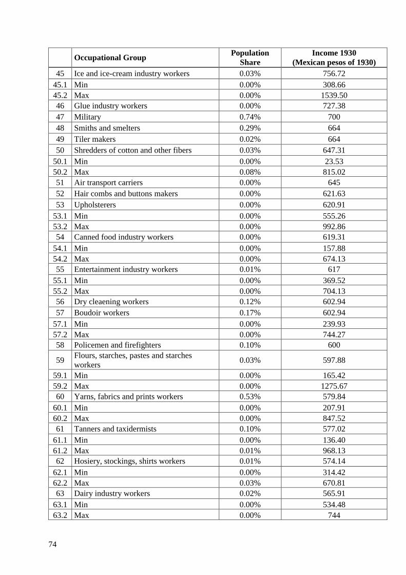
74


Share

Income 1930


45 Ice and ice-cream industry workers 0.03% 756.72

45.1 Min 0.00% 308.66

45.2 Max 0.00% 1539.50

46 Glue industry workers 0.00% 727.38

47 Military 0.74% 700

48 Smiths and smelters 0.29% 664

49 Tiler makers 0.02% 664

50 Shredders of cotton and other fibers 0.03% 647.31

50.1 Min 0.00% 23.53

50.2 Max 0.08% 815.02

51 Air transport carriers 0.00% 645

52 Hair combs and buttons makers 0.00% 621.63

53 Upholsterers 0.00% 620.91

53.1 Min 0.00% 555.26

53.2 Max 0.00% 992.86

54 Canned food industry workers 0.00% 619.31

54.1 Min 0.00% 157.88

54.2 Max 0.00% 674.13

55 Entertainment industry workers 0.01% 617

55.1 Min 0.00% 369.52

55.2 Max 0.00% 704.13

56 Dry cleaening workers 0.12% 602.94

57 Boudoir workers 0.17% 602.94

57.1 Min 0.00% 239.93

57.2 Max 0.00% 744.27

58 Policemen and firefighters 0.10% 600

59 Flours, starches, pastes and starches

workers 0.03% 597.88

59.1 Min 0.00% 165.42

59.2 Max 0.00% 1275.67

60 Yarns, fabrics and prints workers 0.53% 579.84

60.1 Min 0.00% 207.91

60.2 Max 0.00% 847.52

61 Tanners and taxidermists 0.10% 577.02

61.1 Min 0.00% 136.40

61.2 Max 0.01% 968.13

62 Hosiery, stockings, shirts workers 0.01% 574.14

62.1 Min 0.00% 314.42

62.2 Max 0.03% 670.81

63 Dairy industry workers 0.02% 565.91

63.1 Min 0.00% 534.48

63.2 Max 0.00% 744

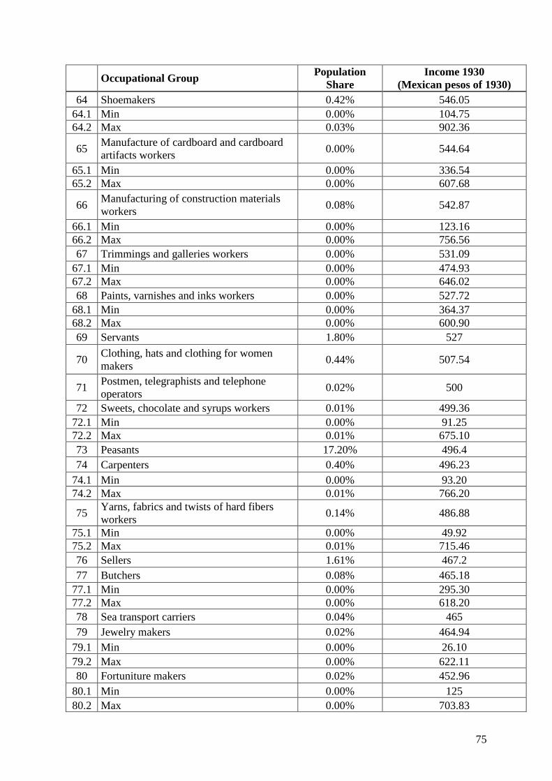
75


Share

Income 1930


64 Shoemakers 0.42% 546.05

64.1 Min 0.00% 104.75

64.2 Max 0.03% 902.36

65 Manufacture of cardboard and cardboard

artifacts workers 0.00% 544.64

65.1 Min 0.00% 336.54

65.2 Max 0.00% 607.68

66 Manufacturing of construction materials

workers 0.08% 542.87

66.1 Min 0.00% 123.16

66.2 Max 0.00% 756.56

67 Trimmings and galleries workers 0.00% 531.09

67.1 Min 0.00% 474.93

67.2 Max 0.00% 646.02

68 Paints, varnishes and inks workers 0.00% 527.72

68.1 Min 0.00% 364.37

68.2 Max 0.00% 600.90

69 Servants 1.80% 527

70 Clothing, hats and clothing for women

makers 0.44% 507.54

71 Postmen, telegraphists and telephone

operators 0.02% 500

72 Sweets, chocolate and syrups workers 0.01% 499.36

72.1 Min 0.00% 91.25

72.2 Max 0.01% 675.10

73 Peasants 17.20% 496.4

74 Carpenters 0.40% 496.23

74.1 Min 0.00% 93.20

74.2 Max 0.01% 766.20

75 Yarns, fabrics and twists of hard fibers

workers 0.14% 486.88

75.1 Min 0.00% 49.92

75.2 Max 0.01% 715.46

76 Sellers 1.61% 467.2

77 Butchers 0.08% 465.18

77.1 Min 0.00% 295.30

77.2 Max 0.00% 618.20

78 Sea transport carriers 0.04% 465

79 Jewelry makers 0.02% 464.94

79.1 Min 0.00% 26.10

79.2 Max 0.00% 622.11

80 Fortuniture makers 0.02% 452.96

80.1 Min 0.00% 125

80.2 Max 0.00% 703.83

76


Share

Income 1930


81 Service sector employees (hotels,

restaurants) 0.02% 450

82 Other industries -0.00% 436.05

82.1 Min 0.00% 81.01

82.2 Max 0.00% 754.48

83 Saddlers 0.04% 434.4

83.1 Min 0.00% 79.91

83.2 Max 0.00% 767.06

84 Vehicle manufacturing workers 0.02% 425.71

84.1 Min 0.00% 73.16

84.2 Max 0.00% 987.17


86 Hunters and fishers 0.04% 420

87 Tonic makers 0.02% 413.92

87.1 Min 0.00% 54.34

87.2 Max 0.00% 486.9

88 Occupations not sufficiently specified 1.25% 407

89 Clothing and hats for men (excluding palm

hats) makers 0.13% 406.34

89.1 Min 0.00% 141.92

89.2 Max 0.00% 549.93

90 Brooches, brushes, brooms, sieves makers 0.00% 391.75

90.1 Min 0.00% 385.07

90.2 Max 0.00% 398.63

91 Attendants 0.10% 387

92 Oils and greases for industrial use makers 0.00% 382.76

92.1 Min 0.00% 253.34

92.2 Max 0.00% 527.95

93 Manufacture and repair of scientific and

precision apparatus workers 0.00% 317.14

94 Dough, tamales, tortillas and atole makers 0.07% 313.93

94.1 Min 0.00% 126.98

94.2 Max 0.01% 656.57

95 Ejidatarios (peasants with communal

property rights) 3.24% 308.57

96 Explosives, gunpowder, pyrotechnics or

rocketry makers 0.02% 304.66

96.1 Min 0.00% 113.25

96.2 Max 0.00% 448.52

97 Potters 0.09% 255.04

97.1 Min 0.00% 22.47

97.2 Max 0.00% 819.89

77


Share

Income 1930


98 Manufacture and repair of musical

instruments 0.00% 143.89

98.1 Min 0.00% 140.83

98.2 Max 0.00% 150

99 Manufacture of art objects. 0.00% 125.21

99.1 Min 0.00% 80.35

99.2 Max 0.00% 160.75

100 Sugar, alcohol and brown sugar or brown

sugar 0.33% 122.03

100.1 Min 0.00% 27.90

100.2 Max 0.00% 342.33


After introducing the regional variations within each category to approximate the maxium level

of within group inequality we get a Gini Index that moves between a minimum level of 0.3097

and a maximum level of 0.5053. Both numbers within a reasonable margin from our prefered

estimates. This excercise can be seen as a robustness check on our 1930 estimates, also

increasing our confidence in the rest of the results.


Table 9: Comparison 1930 (Table 3) vs 1930 (Table 8)

1930 (Table 3) 1930 within inequality (Table 8)

Min 0.3112 0.3097

Max 0.4516 0.5053

Average* 0.3814 0.4075

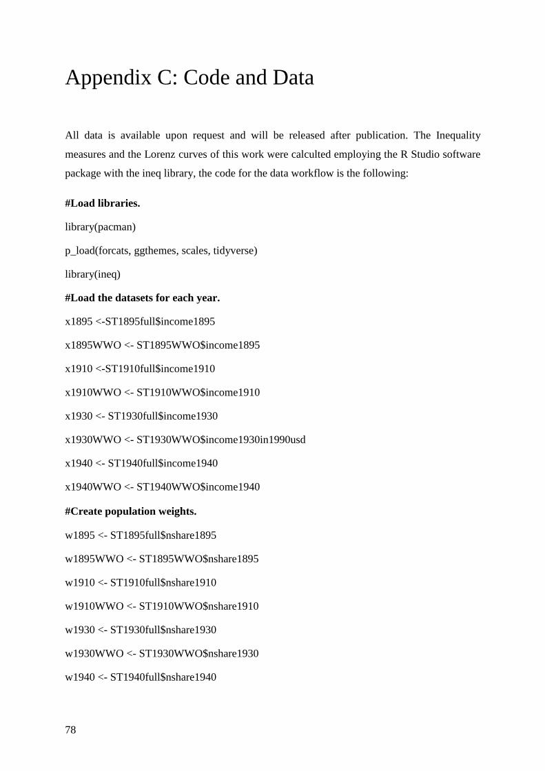
78

Appendix C: Code and Data

All data is available upon request and will be released after publication. The Inequality

measures and the Lorenz curves of this work were calculted employing the R Studio software

package with the ineq library, the code for the data workflow is the following:

#Load libraries.

library(pacman)

p_load(forcats, ggthemes, scales, tidyverse)

library(ineq)

#Load the datasets for each year.

x1895 <-ST1895full$income1895

x1895WWO <- ST1895WWO$income1895

x1910 <-ST1910full$income1910


x1930 <- ST1930full$income1930

x1930WWO <- ST1930WWO$income1930in1990usd

x1940 <- ST1940full$income1940


#Create population weights.

w1895 <- ST1895full$nshare1895

w1895WWO <- ST1895WWO$nshare1895






79


#Gini Index estimation.

weighted.gini(x1895,w1895)

weighted.gini(x1895WWO,w1895WWO)







#Figure 2 code

Lc.max <- Lc.mehran(x1895,w1895)

Lc.max2 <- Lc.mehran(x1910,w1910)

Lc.max3 <- Lc.mehran(x1895WWO,w1895WWO)


plot(Lc.max,col = 8, lty = "twodash", lwd = 4, pch = 1:25,

main = "",

xlab = "Cumulative population", ylab = "Cumulative income")

lines(Lc.max2, col =1, lty = "dashed", lwd = 4, pch = 1:25)

legend("topleft", bg= "transparent", inset = c(.01, .0001), legend=c("1895 max,Gini = .48",

"1895 min Gini = .32", "1910 max Gini = .61", "1910 min Gini = 0.45"),

col=c("gray", "red", "blue", "black"), lty=6:4, cex=.58,text.font=2,box.lty=0, box.lwd=2)

mtext("", side = 1, line = 4, outer = FALSE, at = NA,

adj = 0, padj = NA, cex =0.75, col = "black", font = NA)

lines(Lc.max3, col = 2, lty = "dotted", lwd = 4, pch = 1.25)

lines(Lc.max4, col = 4, lty = "dotdash", lwd = 4, pch = 1.25)

80

#Figure 3 code.




main = "",



legend("topleft",bg= "transparent",inset=.01, legend=c("1895 max,Gini = .48", "1895 min

Gini = .32"),

col=c("gray","black"), lty=6:4, cex=.58,text.font=2,box.lty=0, box.lwd=2)



#Figure 4 code.



plot(Lc.max2,col = 8, lty = "twodash", lwd = 4, pch = 1:25,

main = "",



legend("topleft",bg= "transparent",inset=.01, legend=c("1910 max Gini = .61", "1910 min

Gini = 0.45"),

col=c("black", "gray"), lty=6:4, cex=.58,text.font=2,box.lty=0, box.lwd=2)



81

#Figure 6 code.






main = "",



legend("topleft",bg= "transparent",inset=.0001, legend=c("1930 max,Gini = .45", "1930 min

Gini = .31", "1940 max Gini = .52", "1940 min Gini = 0.41"),

col=c("gray", "red", "blue", "black"), lty=6:4, cex=.58,text.font=2,box.lty=0, box.lwd=2)



lines(Lc.max3, col = 2, lty = "dotted", lwd = 4, pch = 1.25)

lines(Lc.max4, col = 1, lty = "dotdash", lwd = 4, pch = 1.25)

#Figure 7 code.




main = "",



legend("topleft",inset=.01, legend=c("1930 max,Gini = .45", "1930 min Gini = .31"),




82

#Figure 8 code.




main = "",



legend("topleft",inset=.01, legend=c("1940 max,Gini = .52", "1940 min Gini = .41"),




the evolution of inequality in mexico: 1895-1940

Documents