Fe

dera

l Res

erve

Ban

k of

Chi

cago

The Evolution of Comparative Advantage: Measurement and Implications Andrei A. Levchenko and Jing Zhang

November 2014

WP 2014-12

The Evolution of Comparative Advantage: Measurement and

Implications∗

Andrei A. Levchenko

University of Michigan

NBER and CEPR

Jing Zhang

Federal Reserve Bank of Chicago

October 7, 2014

Abstract

We estimate productivities at the sector level for 72 countries and 5 decades, and examine

how they evolve over time in both developed and developing countries. In both country

groups, comparative advantage has become weaker: productivity grew systematically faster

in sectors that were initially at greater comparative disadvantage. These changes have had a

significant impact on trade volumes and patterns, and a non-negligible welfare impact. In the

counterfactual scenario in which each country’s comparative advantage remained the same as

in the 1960s, and technology in all sectors grew at the same country-specific average rate, trade

volumes would be higher, cross-country export patterns more dissimilar, and intra-industry

trade lower than in the data. In this counterfactual scenario, welfare is also 1.6% higher for the

median country compared to the baseline. The welfare impact varies greatly across countries,

ranging from −1.1% to +4.3% among OECD countries, and from −4.6% to +41.9% among

non-OECD countries.

JEL Classifications: F11, F43, O33, O47

Keywords: technological change, sectoral TFP, Ricardian models of trade, welfare

∗We are grateful to the editor (Francesco Caselli), two anonymous referees, Costas Arkolakis, Alan Dear-dorff, Chris House, Francesc Ortega, Dmitriy Stolyarov, Linda Tesar, Michael Waugh, Kei-Mu Yi, and partic-ipants at numerous seminars and conferences for helpful suggestions, and to Andrew McCallum, Lin Ma, andNitya Pandalai Nayar for excellent research assistance. E-mail (URL): alev@umich.edu (http://alevchenko.com),jzhang@chifrb.org (https://sites.google.com/site/jzhangzn/).

1 Introduction

How does technology evolve over time? This question is important in many contexts, most

notably in economic growth and international trade. Much of the economic growth literature

focuses on absolute technological differences between countries. In the context of the one-sector

model common in this literature, technological progress is unambiguously beneficial. Indeed, one

reading of the growth literature is that most of the cross-country income differences are accounted

for by technology, broadly construed (Klenow and Rodrıguez-Clare 1997, Hall and Jones 1999).

By contrast, the Ricardian tradition in international trade emphasizes relative technological

differences as the reason for international exchange and gains from trade. In the presence of multi-

ple industries and comparative advantage, the welfare consequences of technological improvements

depend crucially on which sectors experience productivity growth. For instance, it is well known

that when productivity growth is biased towards sectors in which a country has a comparative

disadvantage, the country and its trading partners may experience a welfare loss, relative to the

alternative under which growth is balanced across sectors. Greater relative technological differ-

ences lead to larger gains from trade, and thus welfare could be reduced when countries become

more similar to each other. This result goes back to at least Hicks (1953), and has been reiterated

recently by Samuelson (2004) in the context of productivity growth in developing countries.1

To fully account for the impact of technological progress on economic outcomes, we must

thus understand not only the evolution of average country-level TFP, but also the evolution of

relative technology across sectors. Or, in the vocabulary of international trade, it is important

to know what happens to both absolute and comparative advantage. Until now the literature

has focused almost exclusively on estimating differences in technology at the country level. This

paper examines the evolution of comparative advantage over time and its implications. Using

a large-scale industry-level dataset on production and bilateral trade, spanning 72 countries, 19

manufacturing sectors, and 5 decades, we estimate productivity in each country, sector, and

decade, and document the changes in comparative advantage between the 1960s and today. We

then use these estimates in a multi-sector Ricardian model of production and trade to quantify

the implications of changing comparative advantage on global trade patterns and welfare.2

Our main results can be summarized as follows. First, we find strong evidence that compar-

ative advantage has become weaker over time. Controlling for the average productivity growth

of all sectors in a country, sectors that had a larger initial comparative disadvantage grew sys-

1Other papers that explore technological change in Ricardian models are, among many others, Jones (1979),Krugman (1979), Brezis, Krugman and Tsiddon (1993), and Hymans and Stafford (1995).

2Technically, the term “comparative advantage” refers to the comparison of autarky prices (Deardorff 1980),and thus encompasses all determinants of relative production cost differences. To streamline exposition, this paperuses “comparative advantage” as a short-hand for “relative sectoral productivity differences,” i.e., the Ricardiancomponent of comparative advantage.

1

tematically faster. This effect is present in all time periods, and is similar in magnitude in both

developed and developing countries. The speed of convergence in sectoral productivities implied

by the estimates is about 18% per decade.

Second, weakening comparative advantage is important for understanding the evolution of

trade volumes and trade patterns. Our quantitative exercise begins by solving the full model under

the actually observed pattern of comparative advantage, and computing all the relevant model

outcomes under this baseline case. We then compare the baseline to a counterfactual scenario in

which each country’s sectoral productivities grow at the same average rate observed between the

1960s and the 2000s, but its comparative advantage remains as it was in the 1960s. Because we

allow average productivity to grow, this exercise isolates the role of changes in comparative – as

opposed to absolute – advantage.

The baseline matches the average trade/GDP ratios observed in the data well. In the coun-

terfactual of unchanged comparative advantage, however, trade volumes as a share of GDP are

15% higher in the 2000s, implying that the rise in trade volumes over the past 5 decades would

have been even higher had comparative advantage not weakened.

Changes in comparative advantage have had an impact on trade patterns as well. We document

that in the data, trade patterns became substantially more similar across countries. In the

majority of sectors, the standard deviation of (log) world export shares across countries has

fallen significantly between the 1960s and the 2000s. In addition, over the same period there has

been a substantial increase in intra-industry trade (measured here by the Grubel-Lloyd index).

As our baseline model is implemented on observed trade flows, it matches these two patterns very

well. By contrast, the counterfactual experiment in which comparative advantage is fixed implies

a much smaller reduction in the dispersion in world export shares, and a much smaller increase

in intra-industry trade than observed in the data.

Finally, these changes in comparative advantage had an appreciable welfare impact. In the

counterfactual scenario of unchanging comparative advantage, in the 2000s the median country’s

welfare would be 1.6% higher than in the baseline. This median welfare impact amounts to nearly

25% of the median gains from trade relative to autarky implied by the model, which are 6.6%.

Moreover, there is a great deal of variation around this average: the percentage difference between

welfare under this counterfactual and the baseline ranges from −1.1% to +4.3% among OECD

countries, and from −4.6% to +41.9% among non-OECD countries. The cross-country dispersion

in the welfare impact of changing comparative advantage is similar to the dispersion in the implied

gains from trade. Lower average welfare is exactly what theory would predict, given the empirical

result that a typical country’s comparative advantage has become weaker over this period.

To estimate productivity, the paper extends the methodology developed by Eaton and Kortum

(2002) to a multi-sector framework. It is important to emphasize the advantages of our approach

2

relative to the standard neoclassical methodology of computing measured TFP. The basic difficulty

in directly measuring sectoral TFP in a large sample of countries and over time is the lack of

comparable data on real sectoral output and inputs.3 By contrast, our procedure uses information

on bilateral trade, and thus dramatically expands the set of countries, sectors, and time periods

for which productivity can be estimated. We follow the insight of Eaton and Kortum (2002) that

trade flows contain information on productivity. Intuitively, if controlling for the typical gravity

determinants of trade, a country spends relatively more on domestically produced goods in a

particular sector, it is revealed to have either a high relative productivity or a low relative unit

cost in that sector. We then use data on factor and intermediate input prices to net out the role

of factor costs, yielding an estimate of relative productivity.

In addition, our approach extends the basic multi-sector Eaton-Kortum framework to incor-

porate many features that are important for reliably estimating underlying technology: multiple

factors of production (labor and capital), differences in factor and intermediate input intensities

across sectors, a realistic input-output matrix between the sectors, both inter- and intra-sectoral

trade, and a non-traded sector. Finally, because our framework allows for international trade

driven by both Ricardian and Heckscher-Ohlin forces, it takes explicit account of each country’s

participation in exports and imports, both of the final output, and of intermediate inputs used in

production.

We are not the first to use international trade data to estimate technology parameters. Eaton

and Kortum (2002) and Waugh (2010) perform this analysis in a one-sector model at a point in

time, an exercise informative of the cross-section of countries’ overall TFP but not their compar-

ative advantage.4 Shikher (2011, 2012) and Costinot, Donaldson and Komunjer (2012) estimate

sectoral technology for OECD countries, while Caliendo and Parro (2014) analyze the impact

of NAFTA in a multi-sector Eaton-Kortum model. Hsieh and Ossa (2011) examine the global

welfare impact of sector-level productivity growth in China between 1993 and 2005, focusing on

the uneven growth across sectors. Chor (2010) relates Ricardian productivity differences to ob-

servable characteristics of countries, such as institutions and financial development. Relative to

existing contributions, we extend the multi-sector approach to a much greater set of countries,

and, most importantly, over time. This allows us, for the first time, to examine not only the

global cross-section of productivities, but also their evolution over the past 5 decades and the

3To our knowledge, the most comprehensive database that can be used to measure sectoral TFP on a consistentbasis across countries and time is the OECD Structural Analysis (STAN) database. It contains the requiredinformation on only 12 developed countries for the period 1970-2008 in the best of cases, but upon closer inspectionit turns out that the time and sectoral coverage is poor even in that small set of countries. Appendix A buildsmeasured TFPs using the STAN database, and compares them to our estimates. There is a high positive correlationbetween the two, providing additional support for the validity of the estimates in this paper.

4Finicelli, Pagano and Sbracia (2009) estimate the evolution of overall manufacturing TFP between 1985 and2002 using a one-sector Eaton and Kortum model.

3

implications of those changes. While existing papers in this literature employ static models, our

quantitative framework features endogenous capital accumulation, and thus permits modeling the

joint evolution of comparative advantage and the capital stock. We show that the response of the

capital stock to changes in comparative advantage has an appreciable welfare impact.

Changes in productivity at the sector level have received comparatively less attention in the lit-

erature. Bernard and Jones (1996a, 1996b) use production data to study convergence of measured

TFP in a sample of 15 OECD countries and 8 sectors, while Rodrik (2013) investigates conver-

gence in value added per worker in an expanded sample of countries. Proudman and Redding

(2000) and Hausmann and Klinger (2007) examine changes in countries’ revealed comparative

advantage and how these are related to initial export patterns. Our paper is the first to use a

fully specified model of production and trade to estimate changes in underlying TFP. In addition,

we greatly expand the sample of countries and years relative to these studies, and use our quan-

titative framework to compute the impact of the estimated changes in comparative advantage on

trade volumes, trade patterns, and welfare.

Our paper is also related to the literature that documents the time evolution of diversification

indices, be it of production (e.g. Imbs and Wacziarg 2003), or trade (e.g. Carrere, Cadot and

Strauss-Kahn 2011). These studies typically find that countries have a tendency to diversify their

production and exports as they grow, at least until they become quite developed. Our findings of

weakening comparative advantage are consistent with greater diversification, and hence provide

a structural interpretation for the evolution of these indices.5

The rest of the paper is organized as follows. Section 2 lays out the theoretical framework.

Section 3 presents the estimation procedure and the data. Section 4 describes the patterns of the

evolution of comparative advantage over time, and presents the main econometric results of the

paper on relative convergence. Section 5 examines the quantitative implications of the observed

evolution of comparative advantage. Section 6 concludes.

2 Theoretical Framework

The world is comprised of N countries and J + 1 sectors. Each sector produces a continuum of

goods. The first J sectors are tradeable subject to trade costs, and sector (J + 1) is nontradeable.

There are two factors of production, labor and capital. Both are mobile across sectors and

immobile across countries. Trade is balanced each period, and thus we abstract from international

asset markets. All agents have perfect foresight and all markets are competitive.

5Our paper is also related to the literature on international technology diffusion, surveyed by Keller (2004).While we document large and systematic changes in technology over time, our approach is, for now, silent onthe mechanisms behind these changes. Section 4.3 relates our empirical results to the theoretical literature ontechnology adoption and diffusion.

4

2.1 Households

In period t = 0, the representative household in country n is endowed with capital Kn0 and

labor Ln0. Each period, the household saves an exogenous fraction snt of its current income (as

in Solow 1956, Swan 1956), investing it into next period’s capital, and consumes the remaining

fraction 1− snt. The saving rates are country-specific and time-varying.6

Period utility of the representative consumer in country n is given by U (Cnt), where Cnt

denotes aggregate consumption in country n and period t. The function U(·) satisfies all the

usual regularity conditions. The flow budget constraint of the household in period t is given by

Pnt (Cnt + Int) = PntYnt = wntLnt + rntKnt, (1)

where Pnt is the price of aggregate consumption, Int is flow saving/investment, Ynt is aggregate

final output, Knt is the capital stock, Lnt is the effective labor endowment, and wnt and rnt are

the wage rate and the rental return to capital, respectively. The budget constraint implicitly

imposes that international trade is balanced in each period. Since investment Int is simply sntYnt,

the law of motion for capital is given by

Knt+1 = (1− δnt)Knt + sntYnt, (2)

where δnt is the country-specific and time-varying depreciation rate.

The aggregate final output Ynt is an aggregate of sectoral composite goods:

Ynt =

J∑j=1

ω1η

j

(Y jnt

) η−1η

ηη−1

ξnt (Y J+1nt

)1−ξnt, (3)

where Y jnt is the composite good in tradeable sector j, and Y J+1

nt is the nontradeable-sector

composite good. The parameter ξnt is thus the Cobb-Douglas weight on the tradeable sector

composite good, η is the elasticity of substitution between the tradeable sectors, and ωj is the taste

parameter for tradeable sector j. The expenditure share on tradeables ξnt varies over time as well

as across countries, to capture in a reduced-form way the positive relationship between income

and the non-tradeable consumption share observed in the data. The aggregate (consumption)

6The variation in snt is meant to capture the influence of demographics, economic growth rates, market frictions,and distortions or subsidies to savings and/or investment due to government policy, or other underlying fundamentaldifferences across countries and over time.

5

price index in country n and period t is thus:

Pnt = Bn

J∑j=1

ωj(pjnt)

1−η

11−η ξnt

(pJ+1nt )1−ξnt ,

where Bn = ξ−ξntnt (1− ξnt)−(1−ξnt) and pjnt is the price of the sector j composite.

2.2 Firms

Output in each sector j and country n and period t is produced using a CES production function

that aggregates a continuum of varieties q ∈ [0, 1] unique to each sector:

Qjnt =

[∫ 1

0Qjnt(q)

ε−1ε dq

] εε−1

,

where ε denotes the elasticity of substitution across varieties q, Qjnt is the total sector j output

in country n, and Qjnt(q) is the amount of variety q that is used in production. It is well known

that the price of sector j’s output is given by:

pjnt =

[∫ 1

0pjnt(q)

1−εdq

] 11−ε

,

where pjnt(q) is the price of variety q in sector j and country n.

The production function of each sectoral variety q is:

yjnt(q) = zjnt(q)(kjnt(q)

1−αj ljnt(q)αj)βj J+1∏

j′=1

mj′jnt (q)γj′j

1−βj

,

where zjnt(q) denotes variety-specific productivity, kjnt(q) and ljnt(q) denote inputs of capital and

labor, and mj′jnt denotes the intermediate input from sector j′ used in producing sector-j goods.

The value-added based labor intensity is given by αj , while the share of value added in total

output is given by βj . Both of these vary by sector. The weights on inputs from other sectors,

γj′j , vary by output industry j as well as input industry j′.

Productivity zjnt(q) for each q ∈ [0, 1] in each sector j and period t is equally available to all

agents in country n, and product and factor markets are perfectly competitive. Following Eaton

and Kortum (2002, henceforth EK), the productivity draw zjnt(q) is random and comes from the

Frechet distribution with the cumulative distribution function

F jnt(z) = e−Tjntz−θ.

6

In this distribution, the absolute advantage term T jnt varies by country, sector, and time, with

higher values of T jnt implying higher average productivity draws in sector j in country n and

period t. The parameter θ captures dispersion, with larger values of θ implying smaller dispersion

in draws.

It will be convenient to define the cost of an “input bundle” faced by sector j producers in

country n:

cjnt =(wαjnt r

1−αjnt

)βj J+1∏j′=1

(pj′

nt

)γj′j1−βj

.

Then, producing one unit of good q in sector j in country n requires 1

zjnt(q)input bundles, and

thus the cost of producing one unit of good q is cjnt/zjnt(q).

International trade is subject to iceberg costs: in order for one unit of good q produced in

sector j to arrive in country n from country i in period t, djnit > 1 units of the good must be

shipped. We normalize djnnt = 1 for each country n and period t in each tradeable sector j.

Note that the trade costs will vary by destination pair, by sector, and time, and need not be

directionally symmetric: djnit need not equal djint. Under perfect competition, the price at which

country i can supply tradeable good q in sector j to country n is equal to:

pjnit(q) =

(cjitzjit(q)

)djnit.

Buyers of each good q in tradeable sector j in country n and period t will select to buy from the

cheapest source country. Thus, the price actually paid for this good in country n will be:

pjnt(q) = mini=1,...,N

{pjnit(q)

}.

Following the standard EK approach, define the “multilateral resistance” term

Φjnt =

N∑i=1

T jit

(cjitd

jnit

)−θ.

This value summarizes, for country n and time t, the access to production technologies in sector

j. Its value will be higher if in sector j, country n’s trading partners have high productivity (T jit)

or low costs (cjit). It will also be higher if the trade costs that country n faces in this sector are

low. Standard steps lead to the familiar result that the probability of importing good q in sector

j from country i in period t, πjnit, is equal to the share of total spending on goods coming from

7

country i, Xjnit/X

jnt, and is given by:

Xjnit

Xjnt

= πjnit =T jit

(cjitd

jnit

)−θΦjnt

.

In addition, the price of good j in country n and period t is simply

pjnt = Γ(

Φjnt

)− 1θ, (4)

where Γ =[Γ(θ+1−εθ

)] 11−ε , and Γ is the Gamma function.

2.3 Equilibrium

The competitive equilibrium of this model world economy consists of sequences of prices,

allocation rules, and trade shares such that (i) given the prices, all firms’ inputs satisfy the

first-order conditions, and their output is given by the production function; (ii) the households’

aggregate consumption and investment decisions are consistent with the exogenous saving rates,

and their sectoral demands satisfy the first order conditions given the prices; (iii) the prices ensure

the market clearing conditions for labor, capital, tradeable goods and nontradeable goods; (iv)

trade shares ensure balanced trade for each country.

The set of prices includes the wage rate wnt, the rental rate rnt, the sectoral prices {pjnt}J+1j=1 ,

and the aggregate price Pnt in each country n and period t. The allocation rules include aggregate

consumption Cnt, investment Int, capital Knt, the capital and labor allocation across sectors

{Kjnt, L

jnt}

J+1j=1 , final demand {Y j

nt}J+1j=1 , and total demand {Qjnt}

J+1j=1 (both final and intermediate

goods) for each sector. The trade shares include the expenditure shares πjnit in country n on goods

coming from country i in sector j.

Characterization of Equilibrium

Given the set of prices {wnt, rnt, Pnt, {pjnt}J+1j=1 }Nn=1, we first characterize the optimal sectoral

allocations from final demand. Consumers maximize utility subject to the budget constraint (1),

(2), and (3). The first order conditions associated with this optimization problem imply the

following final demand across sectors:

pjntYjnt = ξnt(wntLnt + rntKnt)

ωj(pjnt)

1−η∑Jk=1 ωk(p

knt)

1−η, for all j = {1, .., J} (5)

and

pJ+1nt Y J+1

nt = (1− ξnt)(wntLnt + rntKnt).

8

We next characterize the production and factor allocations across the world. Let Qjnt denote the

total sectoral demand in country n and sector j in period t. Qjnt is used for both final demand

and intermediate inputs in domestic production of all sectors. That is,

pjntQjnt = pjntY

jnt +

J∑j′=1

(1− βj′)γjj′(

N∑i=1

πj′

intpj′

itQj′

it

)+ (1− βJ+1)γj,J+1p

J+1nt QJ+1

nt .

Total expenditure in sector j = 1, ..., J + 1 of country n, pjntQjnt, is the sum of (i) domestic final

consumption expenditure pjntYjnt; (ii) expenditure on sector j goods as intermediate inputs in all

the traded sectors∑J

j′=1(1 − βj′)γjj′(∑N

i=1 πj′

intpj′

itQj′

it

), and (iii) expenditure on intermediate

inputs from sector j in the domestic non-traded sector (1− βJ+1)γj,J+1pJ+1nt QJ+1

nt . These market

clearing conditions summarize the two important features of the world economy captured by

our model: complex international production linkages, as much of world trade is in intermediate

inputs, and a good crosses borders multiple times before being consumed (Hummels, Ishii and

Yi 2001); and two-way input linkages between the tradeable and the nontradeable sectors.

In each tradeable sector j, some goods q are imported from abroad and some goods q are

exported to the rest of the world. Country n’s exports in sector j and period t are given by EXjnt =∑N

i=1 1Ii 6=nπjintp

jitQ

jit, and its imports in sector j are given by IM j

nt =∑N

i=1 1Ii 6=nπjnitp

jntQ

jnt, where

1Ii 6=n is the indicator function. The total exports of country n are then EXnt =∑J

j=1EXjnt, and

total imports are IMnt =∑J

j=1 IMjnt. Trade balance requires that for every country n and time

t, EXnt − IMnt = 0.

We now characterize the factor allocations across sectors. The total production revenue in

tradeable sector j in country n and period t is given by∑N

i=1 πjintp

jitQ

jit. The optimal sectoral

factor allocations in country n and tradeable sector j in period t must thus satisfy

N∑i=1

πjintpjitQ

jit =

wntLjnt

αjβj=

rntKjnt

(1− αj)βj.

For the nontradeable sector J + 1, the optimal factor allocations in country n are simply given by

pJ+1nt QJ+1

nt =wntL

J+1nt

αJ+1βJ+1=

rntKJ+1nt

(1− αJ+1)βJ+1.

Finally, the feasibility conditions for factors are given by, for any n,

J+1∑j=1

Ljnt = Lnt and

J+1∑j=1

Kjnt = Knt.

Given all of the model parameters, factor endowments, trade costs, and productivities, the model

is solved using the algorithm described in Appendix B.

9

3 Estimating Model Parameters

This section estimates the sector-level technology parameters T jnt for a large set of countries and

5 decades in three steps. First, we estimate the technology parameters in the tradeable sectors

relative to the U.S. using data on sectoral output and bilateral trade. The procedure relies on

fitting a structural gravity equation implied by the model. This step also produces estimates of

bilateral trade costs at the sector level over time. Second, we estimate the technology parameters

in the tradeable sectors for the U.S.. This procedure requires directly measuring sectoral TFP

using data on real output and inputs, and then correcting measured TFP for selection due to

trade. The taste parameters for all tradeable sectors ωj are also calibrated in this step. Third,

the nontradeable technology is calibrated to match the PPP income per capita in the data.

The calibration of the remaining parameters is more straightforward. Some parameters –

αj , βj , γj′j , snt, ξnt, Lnt, and Knt – come directly from the data. For a small number of parameters

– θ, η, and ε – we take values estimated elsewhere in the literature. Sections 3.1 and 3.2 describe

the estimation of sectoral technology, and Section 3.3 discusses the data sources used in the

estimation as well as the choice of the other parameters.

3.1 Tradeable Sector Relative Technology

Following the standard EK approach, first divide trade shares by their domestic counterpart:

πjnitπjnnt

=Xjnit

Xjnnt

=T jit

(cjitd

jnit

)−θT jnt

(cjnt

)−θ ,

which in logs becomes:

ln

(Xjnit

Xjnnt

)= ln

(T jit(c

jit)−θ)− ln

(T jnt(c

jnt)−θ)− θ ln djnit.

Let the (log) iceberg costs be given by the following expression:

ln djnit = djk,t + bjnit + CUjnit + RTAj

nit + exjit + νjnit,

where djk,t is the contribution to trade costs of the distance between n and i being in a certain

interval (indexed by k). Following EK, we set the distance intervals, in miles, to [0, 350], [350,

750], [750, 1500], [1500, 3000], [3000, 6000], [6000, maximum). Additional variables are whether

the two countries share a common border (which changes the trade costs by bjnit), belong to a

currency union (CUjnit), or to a regional trade agreement (RTAj

nit). We include an exporter fixed

effect exjit following Waugh (2010), who shows that the exporter fixed effect specification does a

10

better job at matching the patterns in both country incomes and observed price levels. Finally,

there is an error term νjnit. Section 4.4 assesses the robustness of the estimates to both the set

of geographic controls and the assumption of the exporter fixed effect in djnit. Note that all the

variables have a time subscript and a sector superscript j: all the trade cost proxy variables affect

true iceberg trade costs djnit differentially across both time periods and sectors. There is a range

of evidence that trade volumes at sector level vary in their sensitivity to distance or common

border (see, among many others, Do and Levchenko 2007, Berthelon and Freund 2008).

This leads to the following final estimating equation:

ln

(Xjnit

Xjnnt

)= ln

(T jit(c

jit)−θ)− θexjit︸ ︷︷ ︸

Exporter Fixed Effect

− ln

(T jnt

(cjnt

)−θ)︸ ︷︷ ︸

Importer Fixed Effect

(6)

−θdjk,t − θbjnit − θCUj

nit − θRTAjnit︸ ︷︷ ︸

Bilateral Observables

−θνjnit︸ ︷︷ ︸Error Term

.

This specification is estimated for each sector and decade separately, allowing for complete flexi-

bility in how the coefficients vary both across sectors and over time. Estimating this relationship

will thus yield, for each country and time period, an estimate of its technology-cum-unit-cost term

in each sector j, T jnt(cjnt)−θ, which is obtained by exponentiating the importer fixed effect. The

available degrees of freedom imply that these estimates are of each country’s T jnt(cjnt)−θ relative

to a reference country, which in our estimation is the United States. We denote this estimated

value by Sjnt:

Sjnt =T jnt

T just

(cjnt

cjust

)−θ,

where the subscript us denotes the United States. It is immediate from this expression that

estimation delivers a convolution of technology parameters T jnt and cost parameters cjnt. Both will

of course affect trade volumes, but we would like to extract technology T jnt from these estimates.

In order to do that, we follow the approach of Shikher (2012). In particular, for each country n,

the share of total spending going to home-produced goods is given by

Xjnnt

Xjnt

= T jnt

(Γcjnt

pjnt

)−θ.

Dividing by its U.S. counterpart yields:

Xjnnt/X

jnt

Xjus,us,t/X

just

=T jnt

T just

(cjnt

cjust

pjust

pjnt

)−θ= Sjnt

(pjust

pjnt

)−θ,

11

and thus the ratio of price levels in sector j relative to the U.S. becomes:

pjnt

pjust=

(Xjnnt/X

jnt

Xjus,us,t/X

just

1

Sjnt

) 1θ

. (7)

The entire right-hand side of this expression is either observable or estimated. Thus, we can

impute the price levels relative to the U.S. in each country and each tradeable sector.

The cost of the input bundles relative to the U.S. can be written as:

cjnt

cjust=

(wntwust

)αjβj ( rntrust

)(1−αj)βj J∏j′=1

(pj′

nt

pj′

ust

)γj′j1−βj (pJ+1nt

pJ+1ust

)γJ+1,j(1−βj)

.

Using information on relative wages, returns to capital, price in each tradeable sector from (7),

and the nontradeable sector price relative to the U.S., we can thus impute the costs of the input

bundles relative to the U.S. in each country and each sector. Armed with those values, it is

straightforward to back out the relative technology parameters:

T jnt

T just= Sjnt

(cjnt

cjust

)θ.

This approach bears a close affinity to development accounting (see, e.g. Caselli 2005). Devel-

opment accounting starts with an observable variable to be accounted for (real per capita income),

and employs other observables – physical capital, human capital, health endowments, etc. – to

absorb as much cross-country variation in the variable of interest as possible. The unexplained

remainder is called TFP. In our procedure, the outcome variable of interest is not income but Sjnt.

Intuitively, if, controlling for the typical gravity determinants of trade, a country spends relatively

more on domestically produced goods in a particular sector – Sjnt is high – it is revealed to have

either a high relative productivity or a low relative factor and input cost in that sector. Just

as in development accounting, we then use measured factor and intermediate input prices to net

out the role of factor and input costs, yielding an estimate of relative productivity as a residual.7

As in development accounting, to reach reliable estimates it is important to net out the impact

of as many observables as possible. Thus, our model features human and physical capital and

sophisticated input linkages, including explicit nontradeable inputs. To accurately reflect sectoral

factor and input cost differences, production function parameters are sector-specific.

7Since our approach uses factor prices rather than factor endowments, it is closer in spirit to the “dual” approachto growth accounting (e.g. Hsieh 2002).

12

3.2 Complete Estimation

So far we have estimated the levels of technology of the tradeable sectors relative to the United

States. To complete our estimation, we still need to find (i) the levels of T for the tradeable

sectors in the United States; (ii) the taste parameters ωj , and (iii) the nontradeable technology

levels for all countries.

To obtain (i), we use the NBER-CES Manufacturing Industry Database for the U.S. (Bartelsman

and Gray 1996). We start by measuring the observed TFP levels for the tradeable sectors in the

U.S.. The form of the production function gives

lnZjust = ln Λjust + βjαj lnLjust + βj(1− αj) lnKjust + (1− βj)

J+1∑j′=1

γj′j lnM j′just, (8)

where Λj denotes the measured TFP in sector j, Zj denotes the output, Lj denotes the labor

input, Kj denotes the capital input, and M j′j denotes the intermediate input from sector j′. The

NBER-CES Manufacturing Industry Database offers information on output, and inputs of labor,

capital, and intermediates, along with deflators for each. Thus, we can estimate the observed

TFP level for each manufacturing tradeable sector using the above equation.

If the United States were a closed economy, the observed TFP level for sector j would be given

by Λjust = (T just)1θ . In the open economies, the goods with inefficient domestic productivity draws

will not be produced and will be imported instead. Thus, international trade and competition

introduce selection in the observed TFP level, as demonstrated by Finicelli, Pagano and Sbracia

(2013). We thus use the model to back out the true level of T just of each tradeable sector in the

United States. Here we follow Finicelli et al. (2013) and use the following relationship:

(Λjust)θ = T just +

∑i 6=us

T jit

(cjitd

jusit

cjust

)−θ.

Thus, we have

(Λjust)θ = T just

1 +∑i 6=us

T jitT just

(cjitd

jusit

cjust

)−θ = T just

1 +∑i 6=us

Sjit

(djusit

)−θ . (9)

This equation can be solved for underlying technology parameters T just in the U.S., given estimated

observed TFP Λjust, and all the Sjit’s and djusit’s estimated in the previous subsection.

To estimate the taste parameters {ωj}Jj=1, we use information on final consumption shares in

the tradeable sectors in the U.S.. We start with a guess of {ωj}Jj=1 and find sectoral prices pj′nt as

follows. For an initial guess of sectoral prices, we compute the tradeable sector aggregate price and

13

the nontradeable sector price using the data on the relative prices of nontradeables to tradeables.

Using these prices, we calculate sectoral unit costs and Φjnt’s, and update prices according to

equation (4), iterating until the prices converge. We then update the taste parameters according

to equation (5), using the data on final sectoral expenditure shares in the U.S.. We normalize the

vector of ωj ’s to have a sum of one, and repeat the above procedure until the values for the taste

parameters converge. This procedure is carried out on the 2000s, and the resulting values applied

to the entire period.

Finally, we calibrate the nontradeable sector TFP in each country to match the observed

PPP-adjusted income per capita. This step involves solving the model with an initial guess of

{T J+1nt }Nn=1 and iteratively updating it until the model-implied income per capita adjusted for the

aggregate price converges to that in the data for each country and each decade. This calibration

approach guarantees that the model produces a cross-country income distribution identical to the

data for each decade.

3.3 Data Description and Implementation

We assemble data on production and trade for a sample of up to 72 countries, 19 manufacturing

sectors, and spanning 5 decades, from the 1960s to the 2000s. Production data come from the

2009 UNIDO Industrial Statistics Database, which reports output, value added, employment, and

wage bills at roughly 2-digit ISIC Revision 3 level of disaggregation for the period 1962-2007 in

the best of cases. The corresponding trade data come from the COMTRADE database compiled

by the United Nations. The trade data are collected at the 4-digit SITC level, and aggregated

up to the 2-digit ISIC level using a concordance developed by the authors. Production and trade

data were extensively checked for quality, and a number of countries were discarded due to poor

data quality. In addition, in less than 5% of country-year-sector observations, the reported total

output was below total exports, and thus had to be imputed based on earlier values and the

evolution of exports.

The distance and common border variables are obtained from the comprehensive geography

database compiled by CEPII. Information on regional trade agreements comes from the RTA

database maintained by the WTO. The currency union indicator comes from Rose (2004), and

was updated for the post-2000 period using publicly available information (such as the membership

in the Euro area, and the dollarization of Ecuador and El Salvador).

In addition to providing data on output for gravity estimation, the UNIDO data are used to

estimate production function parameters αj and βj . To compute αj for each sector, we calculate

the share of the total wage bill in value added, and take a simple median across countries (taking

the mean yields essentially the same results). To compute βj , we take the median of value added

14

divided by total output.

The intermediate input coefficients γj′j are obtained from the Direct Requirements Table

for the United States. We use the 1997 Benchmark Detailed Make and Use Tables (covering

approximately 500 distinct sectors), as well as a concordance to the ISIC Revision 3 classification

to build a Direct Requirements Table at the 2-digit ISIC level. The Direct Requirements Table

gives the value of the intermediate input in row j′ required to produce one dollar of final output

in column j. Thus, it is the direct counterpart of the input coefficients γj′j . In addition, we use

the U.S. I-O matrix to obtain the shares of total final consumption expenditure going to each

sector, which we use to pin down taste parameters ωj in traded sectors 1, ..., J ; as well as αJ+1 and

βJ+1 in the nontradeable sector, which cannot be obtained from UNIDO.8 The baseline analysis

assumes αj , βj , and γj′j to be the same in all countries. Section 4.4 assesses the robustness of the

productivity estimates to allowing these parameters to vary by country.

The total labor force in each country, Lnt, and the total capital stock, Knt, are obtained from

the Penn World Tables 8.0 (PWT8.0). The labor endowment Lnt is corrected for human capital

(schooling) differences using the human capital variable available in PWT8.0. Thus, the wage wnt

captures the relative price of an efficiency unit of labor. The capital series Knt is available directly

in PWT8.0. The saving/investment rate snt is calculated based on the Penn World Tables as the

implied decadal snt that matches the evolution of capital from t to t+1, given real income and the

country-time specific depreciation rate. This approach, together with the fact that our calibration

procedure matched perfectly the relative real per capita incomes for each country, ensures that

the model matches the observed capital stock from period to period.

The computation of relative costs of the input bundle requires information on wages and the

returns to capital. To compute wnt, we take the gross non-PPP adjusted labor income in PWT8.0,

and divide it by the effective endowment of labor, namely the product of the total employment

and the per capita human capital. This yields the payment to one efficiency unit of labor in each

country and decade.

Obtaining information on the return to capital, rnt, is less straightforward, since it is not

observable directly. In the baseline analysis, we impute rnt from the information on the total

income, endowment of capital, and the labor share: rnt = (1−αnt)Ynt/Knt, where the labor share

αnt, total income Ynt, and total capital Knt come directly from the PWT8.0. Since the return to

capital is notoriously difficult to measure, Section 4.4 evaluates the robustness of the estimates

to four alternative ways of inferring rnt.

The price of nontradeables relative to the U.S., pJ+1nt /pJ+1

ust , are computed using the detailed

8The U.S. I-O matrix provides an alternative way of computing αj and βj . These parameters calculated basedon the U.S. I-O table are very similar to those obtained from UNIDO, with the correlation coefficients betweenthem above 0.85 in each case. The U.S. I-O table implies greater variability in αj ’s and βj ’s across sectors thandoes UNIDO.

15

price data collected by the International Comparison of Prices Program (ICP). For a few countries

and decades, these relative prices are extrapolated using a simple linear fit to log PPP-adjusted

per capita GDP from the Penn World Tables.

In order to estimate the relative TFP’s in the tradeable sectors in the U.S., we use the 2009

version of the NBER-CES Manufacturing Industry Database, which reports the total output,

total input usage, employment, and capital stock, along with deflators for each of these in each

sector. The data are available in the 6-digit NAICS classification for the period 1958 to 2005,

and are converted into ISIC 2-digit sectors using a concordance developed by the authors. The

procedure yields sectoral measured TFP’s for the U.S. in each tradeable sector j = 1, ..., J and

each decade.

The share of expenditure on traded goods, ξnt in each country and decade is sourced from Uy,

Yi and Zhang (2013), who compile this information for 30 developed and developing countries.

For countries unavailable in the Uy, Yi and Zhang data, values of ξnt are imputed based on fitting

a simple linear relationship to log PPP-adjusted per capita GDP from the Penn World Tables.

In each decade, the fit of this simple bivariate regression is typically quite good, with R2’s of 0.30

to 0.80 across decades.

The baseline analysis assumes that the dispersion parameter θ does not vary across sectors

and sets θ = 8.28, which is the preferred estimate of EK. Section 4.4 shows that the productivity

estimates are quite similar under two alternative sets of assumptions on θ: (i) a lower value of

θ = 4, and (ii) sector-specific values of θj .

We choose the elasticity of substitution between broad sectors within the tradeable bundle, η,

to be equal to 2. Since these are very large product categories, it is sensible that this elasticity

would be relatively low. It is higher, however, than the elasticity of substitution between tradeable

and nontradeable goods, which is set to 1 by the Cobb-Douglas assumption. The elasticity of

substitution between varieties within each tradeable sector, ε, is set to 4 (as is well known, in the

EK model this elasticity plays no role, entering only the constant Γ).

Appendix Table A1 lists the countries used in the analysis along with the time periods for

which data are available for each country, and Appendix Table A2 lists the sectors along with

the key parameter values for each sector: αj , βj , the share of nontradeable inputs in total inputs

γJ+1,j , and the taste parameter ωj . All of the variables that vary over time are averaged for

each decade, from the 1960s to the 2000s, and these decennial averages are used in the analysis

throughout. Thus, our unit of time is a decade.

16

4 Evolution of Comparative Advantage

This section describes the basic patterns in how estimated sector-level technology varies across

countries and over time, focusing especially on whether comparative advantage has become

stronger or weaker. Going through the steps described in Section 3.1 yields, for each country

n, tradeable sector j, and decade t, the state of technology relative to the U.S., T jnt/Tjust. Since

mean productivity in each sector is equal to (T jnt)1/θ, we carry out the analysis on this exponen-

tiated value, rather than T jnt.

4.1 Basic Patterns

Table 1 presents summary statistics for the OECD and non-OECD countries in each decade. The

first column reports the mean productivity relative to the U.S. across all sectors in a country, a

measure that can be thought of as absolute advantage. The OECD countries as a group catch

up to the U.S. between the 1960s and the 2000s, with productivities going up from 0.91 to in

excess of 1 over the period. The non-OECD countries’ productivity is lower throughout, but

the catch-up is also evident. The second column in each panel summarizes the magnitude of

within-country differences in productivity across sectors, i.e., the coefficient of variation of sectoral

productivities within a country, averaged by country group and decade. This measure can be

thought of as comparative advantage across sectors. The average coefficient of variation is about

50% lower in the OECD countries compared to the non-OECD, reflecting higher dispersion of

sectoral productivities in poorer countries, or “stronger comparative advantage.” In both country

groups, there is a clear downward trend in the coefficient of variation, which is first evidence

that comparative advantage is getting weaker over time – sectoral relative productivity dispersion

within a country is falling.

The bottom panel presents the same statistics but balancing the country sample across

decades. There are virtually no changes for the OECD, since the OECD sample is more or less

balanced to begin with. For the non-OECD, balancing the sample implies dropping 19 countries

in later decades, but the basic patterns are unchanged.

The evolution of these averages over time masks a great deal of heterogeneity among countries.

To visualize this heterogeneity, Figures 1(a) and 1(b) plot the changes in the average T 1/θ against

their initial average values. The left panel does this from the 1960s to the 2000s, the right panel

from the 1990s. These plots can be thought of as capturing the traditional (cross-country) notion

of absolute convergence. There is quite a bit of dispersion in the extent to which countries caught

up on average to U.S. productivity, including a few countries that fell behind on average relative

to the U.S.. There is an apparent negative relationship between the extent of catch-up and the

initial average level, stronger from the 1990s.

17

Figures 1(c) and 1(d) plot the within-country dispersions of productivities (the coefficients

of variation) in the 2000s against their values in the 1960s and the 1990s, respectively. For

convenience, 45-degree lines are added to these plots. There is a fair amount of cross-country

variation in productivity dispersion, and this variation appears to be persistent over time. Since

the 1960s, sectoral productivity dispersion fell in the majority of countries (in all but 13). Between

the 1990s and the 2000s, there is no systematic fall in dispersion: Table 1 shows that the coefficient

of variation actually rises on average between those two decades in both groups of countries.

4.2 Relative Convergence

To shed further light on whether comparative advantage has gotten stronger or weaker over time,

we estimate a convergence specification in the spirit of Barro (1991) and Barro and Sala-i-Martin

(1992):

∆ log(T jn)1/θ

= βInitial log(T jn)1/θ

+ δn + δj + εnj . (10)

Unlike the classic cross-country convergence regression, our specification pools countries and sec-

tors. On the left-hand side is the log change in the productivity of sector j in country n. The

right-hand side regressor of interest is its beginning-of-period value. All of the specifications in-

clude country and sector fixed effects, which affects the interpretation of the coefficient. The

country effect absorbs the average change in productivity across all sectors in each country – the

absolute advantage. Thus, β picks up the impact of the initial relative productivity on the relative

growth of a sector within a country – the evolution of comparative advantage. In particular, a

negative value of β implies that relative to the country-specific average, the most backward sectors

grew fastest.

Table 2 presents the results. The first column reports the coefficients for the longest differences:

the 1960s to the 2000s, while the second column estimates the specification starting in the 1980s.

The following 4 columns carry out the estimation decade-by-decade, 1960s to 1970s, 1970s to

1980s, and so on. Since the length of the time period differs across columns, the coefficients

are not directly comparable. To help interpret the coefficients, underneath each one we report

the speed of convergence, calculated according to the standard Barro and Sala-i-Martin (1992)

formula: β = e−λT − 1, where β is the regression coefficient on the initial value of productivity, Tis the number of decades between the initial and final period, and λ is the convergence speed. This

number gives how much of the initial difference between productivities is expected to disappear

in a decade. All of the standard errors are clustered by country, to account for unspecified

heteroscedasticity at the country level. All of the results are robust to clustering instead at the

sector level, and we do not report those standard errors to conserve space.9

9If the initial T ’s tend to be measured with error, it has been noted that the convergence regression of the

18

Column 1 of the top panel reports the estimates for the long-run convergence in the pooled

sample of all countries. The coefficient is negative, implying that there is convergence: within a

country, the weakest sectors tend to grow faster. It is highly statistically significant: even with

clustered standard errors the t-statistic is nearly 12. The speed of convergence implied by this

coefficient is 18% per decade. As a benchmark, the classic Barro and Sala-i-Martin (1992) rate of

convergence is 2% per year, or 22% per decade, close to what we find in a very different setting.

The second column estimates the long-difference specification from the 1980s to the 2000s. Once

again, the coefficient is negative and highly significant, but it implies a considerably slower rate

of convergence, 11.7% per decade. The rest of the columns report the results decade-by-decade.

Though there is statistically significant convergence in each decade, the speed of convergence

trends downward, from 26% from the 1960 to the 1970s, to 11.4% in the most recent period.

In order to assess how the results differ across country groups, Panels B and C report the

results for the OECD and the non-OECD subsamples separately. Breaking it down produces

slightly faster convergence rates than in the full sample. In the decade-to-decade specifications,

the non-OECD countries are catching up somewhat faster, which is not surprising.

Figures 2 and 3 present the results graphically. Figure 2 plots the unconditional bivariate

relationship between the log change in productivity and the log initial level in each sector. Within

most sectors, the negative relationship is evident. In every sector, the estimated coefficient is

negative, and in 14 of the 19 sectors, it is significant at the 5% level. Figure 3 plots the partial

correlation between the initial level and subsequent growth, after netting out country and sector

fixed effects. This is the partial correlation plot underlying the first coefficient reported in Table

2. Once again, the negative relationship is evident in the pooled sample.

Appendix Tables A3 reports the results of estimating the convergence equation (10) country

by country from the 1960s to today. These results should be treated with more caution, as the

sample size is at most 19. The columns report the coefficient, the standard error, the number

of observations, the R2, as well as the implied speed of convergence for each country. There

is considerable evidence of convergence in these country-specific estimates. In all countries, the

type estimated here will produce bias in favor of finding convergence (Quah 1993). We ran a number of checks toassess the relevance of this effect in our setting. First, we estimated a number of panel specifications with a varietyof interacted fixed effects: country×sector, country×decade, and sector×decade included together in estimation.These additional fixed effects will help control for measurement error that varies mainly at country-sector, country-time, or sector-time level, respectively. We also implemented the Arellano-Bond and Blundell-Bond dynamic panelestimators, that difference the data and use lagged values of T to instrument for current changes in T . All ofthese alternative estimates actually imply a faster speed of convergence than the estimates in Table 2. Second,to check how much measurement error is needed to generate our results, we ran a simulation in which we startedwith artificial data exhibiting zero convergence across sectors within a country, and added measurement error tothe right-hand side variable until the OLS coefficient was equal to the coefficient found in our estimates. It turnsout that in order for measurement error to produce coefficient magnitudes found in the data when the truth is zeroconvergence, it must be the case that 62% of the cross-sectoral variation in the right-hand side variable is due tomeasurement error.

19

convergence coefficient is negative, and significant at the 10% level or below in 38 out of 50

available countries (76%).

All in all, these results provide robust evidence of relative convergence: in all time periods

and broad sets of countries we consider, relatively weak sectors grow faster, with sensible rates of

convergence. This implies that Ricardian comparative advantage is getting weaker, at least when

measured at the level of broad manufacturing sectors.

4.3 Discussion

A large literature in growth, synthesized by Acemoglu (2008, Ch. 18), studies aggregate country-

level technology differences using multi-country models of technology adoption. This literature

has pursued two broad directions. The first postulates that aggregate productivity differences

persist because there are frictions in technology adoption. In order to ensure a stable world

income distribution, a central assumption in this type of framework is that countries farther

behind the world productivity frontier find it easier to increase productivity. This hypothesis

dates back to Gerschenkron (1962), and is typically introduced as a reduced-form relationship

in these models. The second approach postulates that all technologies are freely available to all

countries at all times, but due to capital and/or skill endowment or institutional differences, poorer

countries cannot make the best use of the available technologies (Atkinson and Stiglitz 1969, Basu

and Weil 1998, Acemoglu and Zilibotti 2001, Caselli and Coleman 2006, Acemoglu, Antras and

Helpman 2007).

Since these models are framed in terms of aggregate technology differences, they are challenging

to evaluate empirically. This is because at the country level, it is difficult to distinguish between

the role of distance to the world frontier and other country-specific factors, especially when these

factors themselves condition the speed of productivity convergence. By opening up a sectoral

dimension, our results can provide some empirical evidence on these theories. Our convergence

regressions include country fixed effects, and thus control for country-specific determinants of

productivity growth affecting all the sectors equally. Though our convergence coefficients capture

the notion of within-country convergence, they nonetheless lend support to the key assumption

in models of slow technology diffusion: it is easier to catch up starting from a more backward

position.

The second approach rationalizes persistent technology gaps by appealing to the appropri-

ateness of world frontier technologies for local country conditions, such as the capital-labor ratio

(Atkinson and Stiglitz 1969, Basu and Weil 1998), skill endowment (Acemoglu and Zilibotti 2001,

Caselli and Coleman 2006), or institutional quality (Acemoglu et al. 2007). While our results are

not geared to informing or testing these theories, we can use the variation in the country-specific

20

convergence coefficients in Appendix Table A3 to look for some supporting evidence. Once again,

the mapping to existing theories is inexact: our results capture within-country, cross-sectoral speed

of convergence, whereas the theoretical literature is about cross-country differences. In addition,

variation across sectors in some relevant attributes, such as capital or skill intensity, may play a

role as well. Nonetheless, there are some modest but suggestive patterns. The country-specific

speed of convergence reported in Appendix Table A3 is positively correlated with the country’s

capital-labor ratio (correlation 0.54), skill endowment (correlation 0.29), and institutional quality

(correlation 0.47).10 Of course, these three country characteristics are highly positively correlated,

and thus distinguishing between the alternative theories using our data is impractical. However,

the positive correlations are suggestive that country characteristics do matter for the speed of

technology adoption in ways predicted by theory.

In contrast to the aggregate productivity literature, theories of the dynamics of sectoral tech-

nology and Ricardian comparative advantage are quite scarce. Krugman (1987) and Young (1991)

develop learning-by-doing models of comparative advantage. A strong implication of these models

is that relative productivity differences increase over time – comparative advantage strengthens.

This is because learning is faster in sectors that produce more, and comparative advantage sectors

are the ones that produce more. Our results are clearly inconsistent with the main prediction of

the learning-by-doing models, at least not at the level of broad sectors. Similarly, Grossman and

Helpman (1991, Ch. 8) develop a model with a traditional and a knowledge-based sector, and

show that one country’s initial advantage in the stock of R&D leads to an increasingly stronger

comparative advantage in the knowledge-based sector. Once again, our findings of pervasive

convergence in productivity do not support this type of theoretical prediction.

A theoretical and quantitative framework with endogenous sectoral productivity that can be

used for understanding the empirical patterns we identify is yet to be developed, and remains a

potentially fruitful direction for future research. One promising possibility is the framework of

“defensive innovation” in response to import competition recently developed by Bloom, Romer,

Terry and Van Reenen (2012) (see also Bloom, Draca and Van Reenen 2011).

4.4 Robustness of T Estimates

This section presents a battery of robustness checks on our productivity estimation procedure.

The outcomes are summarized in Appendix Table A4. The table reports the mean productivity

T 1/θ relative to the U.S., its standard deviation across countries and sectors, the correlation with

the baseline productivity estimates across countries and sectors, and the convergence coefficient

10These correlations are computed after dropping the 3 outlier countries with the highest speed of convergencepoint estimates. Without dropping outliers, the correlations are 0.40, 0.31, and 0.42, respectively. The institutionalquality index is “Rule of Law” sourced from the World Bank’s Governance Matters Database.

21

and standard error from the main regression specification (10), estimated on the alternative sets

of productivity estimates. To ease comparison, the top row reports the values for the baseline

T 1/θ estimates.

The first set of checks concerns the specification of the gravity equation (6). To assess whether

the estimates are sensitive to the set of distance and gravity variables included in estimation, we

repeat the analysis while doubling the set of distance intervals (from 6 to 12), and including

standard additional controls for common language and colonial ties, which are absent from the

baseline specification. As the row labeled “Additional gravity” reveals, the resulting productivity

estimates and convergence results are virtually indistinguishable from the baseline.

Next, we estimate the gravity equation in levels using the Poisson Pseudo Maximum Likelihood

approach suggested by Santos Silva and Tenreyro (2006). This has the convenient property of

not dropping zero trade observations from the estimation sample. The results are once again very

similar to the baseline across the board.11

The next robustness check concerns whether the trade cost specification includes an exporter

or an importer effect. Waugh (2010) appeals to tradeable prices to argue that the specification

with an exporter fixed effect fits the data better. In particular, he documents that in the data,

tradeable prices are weakly increasing in income. The model with the exporter fixed effect in

djnit can match this pattern. However, the model with the importer fixed cost in djnit delivers

the sharply counterfactual prediction that tradeable prices fall in income. In addition, Waugh

(2010) shows that the importer fixed effect specification does less well in other dimensions, such

as matching observed income differences between countries.

Though we employ a very different model than Waugh (2010) – most importantly, we have

multiple tradeable sectors, an explicit non-tradeable sector, and input linkages between those –

his argument applies in our setting as well, albeit in a milder form. Just as in Waugh (2010), our

baseline model with exporter effects in djnit delivers a flat tradeable prices-income relationship,

11A standard feature of the baseline procedure is that the trade shares are logged, so that the zero bilateral importflows are dropped from the estimation sample. Unfortunately, our large-scale model cannot be tractably enriched toexplicitly account for zeros in trade while at the same time retaining the structural interpretation linking the fixedeffects to underlying productivity. However, we can check the ex-post performance of the estimated model withrespect to zeros by solving the full model, and computing within the model the sum of the πjnit’s in the importer-exporter-sector observations that are zeros in the actual data. We can then examine whether these observationsaccount for large shares of absorption inside the model. If the resulting numbers are large, then the quantitativemodel predicts substantial trade flows where in reality they are zero. However, if these numbers are small, the modelpredicts very small flows where the actual flows are zero, providing a good approximation to the data even thoughbaseline productivities are estimated dropping zero trade. The results of this exercise are reported in AppendixTable A5. The exercise takes the most expansive view of the zeros, by assuming that all trade flows missing inthe data are actually zeros as well. Observations for which the data exhibit zero/missing trade flows account for atiny share of overall absorption in our quantitative model: in each decade, these observations add up to on averageless than 0.9% of the total absorption. Breaking down across sectors and decades, we see that nearly all individualsectors or decades, these shares are small. We conclude from this exercise that in spite of ignoring the zero tradeobservations in estimation, our quantitative model is quite close to the data when it comes to small/zero tradeflows.

22

matching the data. By contrast, when we re-estimate the model with importer effects in djnit, it

implies a negative relationship between tradeable prices and income.

Nonetheless, we present the results of re-estimating sectoral productivities based on the im-

porter effects in djnit assumption. The results, presented in row “imjnt in djnit” reveal that the

average productivities implied by this alternative approach are lower (0.53 at the mean compared

to 0.74 for the baseline). However, the dispersion in those productivities is very similar to the

baseline, and the two sets of estimates have a correlation of 0.89. Most importantly, the rela-

tive convergence result is clearly evident in these estimates, though the speed of convergence is

somewhat slower than in the baseline.

The second set of robustness checks concerns the measurement of the return to capital rnt,

that enters the unit cost terms cjnt, and thus the productivity estimates. The baseline computes

rnt using data on Knt, the total income Ynt, and the (country- and time-specific) labor share.

However, the return to capital is notoriously difficult to measure, and thus we perform a battery

of robustness checks on rnt. First, we use the Caselli and Feyrer (2007) correction for natural

wealth. The data for natural wealth are for 1995-2005, and come from the World Bank. Even for

this later period, not all countries in our baseline sample are covered. In addition, these data are

not available before 1995, which forces us to apply the 1995 values to all preceding decades.

Second, we use a measure of the return to capital computed instead from consumption growth.

Namely, we exploit the Euler equation in consumption to back out the rate of return on capital:

1+rnt+1−δnt = U ′(Cnt+1)ρU ′(Cnt)

, with ρ the discount factor. We use Penn World Tables data on consump-

tion and the country-specific depreciation rate δnt, and the standard functional form/parameter

assumptions, namely CRRA utility U(C) = C1−σ

1−σ , with σ = 2 and annual ρ = 0.96. The results

are reported in row labeled “Euler.”

Third, we use data on lending interest rates from the World Development Indicators. This

approach yields a 20% smaller sample of countries and decades. The results are in the row

labeled “Direct.” And finally, we adopt the simple assumption that rnt is the same everywhere

in the world at a point in time (rnt = rust ∀n, t). This assumption can correspond to financial

integration, for instance. Caselli and Feyrer (2007) show that at least as of the 1990s, this is not

a bad assumption. The results are in the row “Fin. Integration.”

The means and standard deviations of estimated productivities under these four alternative

approaches do not differ much from the baseline. The correlations to the baseline are also quite

high, from 0.91 under the direct measurement to 0.99 under the Caselli-Feyrer correction. The

convergence results are also equally strong under these alternative approaches of measuring rnt.

Next, we check the sensitivity of the results to the assumption that the production functions

(IO matrices and factor shares) are the same across countries. The row “Country-Specific IO”

presents the results of estimating productivities using country-specific IO matrices sourced from

23

GTAP. GTAP’s coverage of sectors and countries is not the same as in our analysis, requiring some

imputation, and thus we do not use these in the baseline analysis. The row “Country-Specific IO,

α, β” in addition assumes that the labor share in value added (α) and the share of value added

in output (β) are vary by country and decade (and of course, as always, by sector). We compute

these directly for each sector, country, and decade using UNIDO data on the wage bill, value

added, and output. We do not use these values in the baseline analysis, because the UNIDO data

do not have complete coverage, requiring some imputation. In addition, it can be noisy, and thus

variation in these empirical factor shares across countries and over time may not provide a reliable

indication of true differences in factor intensity. These two alternative approaches yield slightly

higher average productivities, but the variation is similar to the baseline and the correlations are

very high. The convergence results are also equally strong.

The final set of checks is on the θ parameters. First, one may be concerned about how the

results change under lower values of θ. Lower θ implies greater within-sector heterogeneity in

the random productivity draws. Thus, trade flows become less sensitive to the costs of the input

bundles (cjnt), and the gains from intra-sectoral trade become larger relative to the gains from

inter-sectoral trade. We repeated the estimation assuming instead a value of θ = 4, which has

been advocated by Simonovska and Waugh (2014) and is at or near the bottom of the range

that has been used in the literature. Overall, the results are remarkably similar. The mean

productivities are virtually the same, and there is actually somewhat greater variability in T jnt’s

under θ = 4. The correlation between estimated T jnt’s under θ = 4 and the baseline is above 0.94.

The convergence results are equally strong.

Second, a number of studies have suggested that θ varies across sectors (see, e.g., Chen and

Novy 2011, Caliendo and Parro 2014, Imbs and Mejean 2014). We repeat the estimation allowing

θj to be sector-specific, with sectoral values of θj sourced from Caliendo and Parro (2014). The

average productivities are once again quite similar, and have an 0.87 correlation with the baseline.

The convergence results are if anything stronger than in the baseline.

Another important question is whether our estimates can be cross-validated using direct es-

timates of measured TFP. Appendix A estimates measured TFP using data on real output and

inputs from the OECD Structural Analysis database. It is the most comprehensive database that

contains the information required to estimate measured TFP on a consistent basis across countries

and over time. Using both simple correlations and regression estimates with fixed effects, we con-

firm that our baseline estimates indeed exhibit a close positive association with TFP calculated

based on STAN data.

24

4.5 Simple Heuristics: What is Driving the Convergence Finding?

What kinds of basic patterns in the data are driving these results? Though our estimation

procedure is based on a theoretically-founded gravity equation and a variety of data sources,

and thus is fully internally consistent with the underlying conceptual framework, it would be

reassuring if we could show some simple heuristic relationships in the data that are consistent

with weakening comparative advantage. We can build intuition as follows: in a simpler model

with 2 tradeable and 1 nontradeable sectors, Uy et al. (2013) show analytically that all else

equal, a comparative advantage sector has a smaller share of imports in total domestic absorption

1−πjnn than a comparative disadvantage sector. As a country’s comparative advantage in sector j

weakens, the import share rises in that sector. This is intuitive: when a country becomes relatively

less productive in a sector, it starts importing more.

Thus, weakening comparative advantage should manifest itself in a negative relationship be-

tween the initial period import share and the subsequent change in the import share. Sectors

within a country with the lowest initial import share (1− πjnn) should see that import share rise.

These are the sectors with the strongest comparative advantage at the beginning of the period.

Correspondingly, sectors with the highest initial import share should see their import share drop

as they catch up in productivity faster.

Figure 4(a) presents this scatterplot, pooling sectors and countries. The negative relationship

is remarkably pronounced: the slope coefficient in the simple bivariate regression is −0.397 with

a t-statistic of 16.5 and an R2 of 18.4%. Note that a significant share of the observations – those

below zero on the y-axis – have seen their import share actually fall between the 1960s and today.

These declines in import shares would be highly puzzling over the period during which trade

costs fell and global trade volumes rose dramatically. A strengthening of comparative advantage

in those sectors provides a plausible explanation: countries are getting relatively better in those

industries, and thus they need to import less.

This negative relationship would not necessarily be evidence of relative convergence in the

T ’s if, for instance, trade costs djnit fell disproportionately more in sectors in which countries had

higher initial import shares. To check for this possibility, Figure 4(b) plots the change in the

average trade costs in sector j and country n against the initial import share – the same x-axis

variable as in the previous figure. There is virtually no relationship between initial import share

and subsequent changes in import costs: the slope coefficient is essentially zero, and the R2 is

correspondingly 0.00. Thus, it does not appear that systematically larger reductions in djnit in

the initial comparative disadvantage sectors were primarily responsible for the pattern in Figure

4(a). Note that our estimation procedure is designed precisely to take into account any changes

in djnit (as well as unit factor costs) by importer-exporter pair and sector that may have occurred

25

over this period, isolating the underlying productivity changes.

5 Quantitative Implications

This section computes the global impact of changes in comparative advantage documented in the

previous section. In order to do this, we solve the full model laid out in Section 2 for a variety

of values of technology parameters. The main goal of the exercise is to compare outcomes in the

world as we see it today to a counterfactual world in which average productivities remain as they

are in the data, but relative sectoral productivities are fixed to their initial values. The outcomes

we are interested in are trade volumes and patterns, and welfare/real incomes.

Our framework features endogenous capital accumulation. Thus, to model the counterfactual

world in which comparative advantage is fixed, we must track what happens to capital in each

decade in this case. Our results thus also reflect the impact of changing comparative advantage

on capital accumulation over the past 5 decades.

5.1 Benchmark Results and Model Fit

The baseline corresponds to the actual values of T jnt estimated for the past five decades. Before

running the counterfactual experiments, we assess the fit of the baseline model in a number of

dimensions. By construction, the model matches perfectly the real PPP-adjusted per capita

income in each country. Table 3 compares w’s and r’s in the model and in the data for 2000s.

(The results for the previous decades are similar.) The baseline model performs well: the means

and the medians match up fairly well, and the correlation between model and data wages is 0.95.

The correlation in r’s is somewhat lower at 0.59.

The next panel assesses the model’s ability to match the sectoral trade flows. It reports the

means and medians, across countries and sectors, of πjnnt. The model reproduces the overall

magnitudes well, and the correlation between the model and the data is 0.92. The same can be

said for the cross-border flows πjnit, i 6= n, reported in the bottom panel.

5.2 Counterfactual Comparative Advantage

In the counterfactual experiments, we solve the model while keeping comparative advantage fixed

to the 1960s. Thus, the counterfactual exercise assumes that for each decade t after the 1960s, each

country’s sectoral productivities relative to the world frontier grew at their geometric average rate,

but comparative advantage remained the same as it was in the 1960s. Precisely, the counterfactual

26

T ’s are calculated as:

T jnt

T jF t=T jn1960s

T jF1960s

×

(∏Jk=1

TkntTkFt

) 1J

(∏Jk=1

Tkn1960sTkF1960s

) 1J

,

where T jF t is the world frontier in sector j at decade t. In each sector and decade, we select the

2 highest values of T jnt/Tjust, take their geometric mean, and label that the global frontier. We

then compute each country’s technology parameters in the counterfactual with reference to this

frontier productivity.

The use of geometric averages has two appealing features. The first is that even though the

counterfactual T ’s are calculated to keep their distance to the frontier, the geometric average

of counterfactual T ’s is equal to the geometric average of the country’s actual T ’s at every t.

This ensures that the normalization to the frontier does not induce movements up or down of

the average productivity in the country, which would confound the meaning of our counterfactual

exercise. The second appealing feature is that this formulation produces identical counterfactual

T ’s whether the experiment is carried out on absolute T ’s or T 1/θ’s, which are the mean pro-

ductivities. We keep productivity in the nontradeable sector at the benchmark value in all the

counterfactual experiments, since our focus is on the welfare impact of changes in comparative

advantage. Thus, an additional feature of the counterfactual design is that the productivity of

tradeables relative to nontradeables is also fixed throughout.

We perform two variants of this counterfactual experiment. The first, labeled “global,” keeps

relative productivities at their 1960s values for all countries in the world simultaneously. This

counterfactual is best suited for evaluating the worldwide consequences of the observed global

productivity convergence. The second, “single-country,” keeps relative productivities at their

initial values for one country at a time, while the rest of the world has their baseline estimated

productivities. This counterfactual is ideal for evaluating the consequences for each country of

changes in its own comparative advantage.

Countries that join the sample later than the 1960s in the counterfactuals keep their relative

productivities fixed to the first decade they are in the data. We think of those initial productivities

as our best guess for their pattern of comparative advantage as of the 1960s.

5.3 Trade Volumes and Trade Patterns

We begin with the discussion of the impact of changing comparative advantage on observable

outcomes, namely international trade volumes and patterns. Table 4 presents the results. The

first column reports the value of each moment in the data, the second in the benchmark model, and

the third and fourth in the global and single-country counterfactuals, respectively. The numbers

27

in italics under the averages are the correlations across countries in each moment between the

model and the data.

The first row assesses the impact of changes in comparative advantage on trade volumes.

It reports the average manufacturing imports/GDP ratio in the 2000s across the countries in

the sample. The mean in the benchmark model matches that in the data almost perfectly, and

the correlation between the two is also high at nearly 0.6. The next two columns report the

manufacturing import/GDP ratio for the two counterfactuals. It is clear that in the absence of

changes in relative productivities, world trade volumes would be even higher than they are today.

The difference is sizable: imports to GDP would be 3.7 percentage points higher if all countries

kept their initial relative productivities, a 15% difference.

Next, we look at trade patterns rather than trade volumes, and examine whether the model

can match the long-run changes observed in the data. One sharp pattern in the data is that within

a sector, export volumes are becoming more similar across countries over time. This is captured in

the table by the change in the standard deviation of log shares of world exports within a particular

sector across countries. The first column shows that in the data it has decreased systematically

between the 1960s and today. While the table reports the cross-sectoral average, this pattern

is also pervasive: in 17 out of 19 sectors, the dispersion of log country shares of world exports

has fallen. The next column reports the same statistic in the benchmark model, as well as the

correlation across sectors between the model and the data. The model matches quite well both the

overall decrease, and the cross-sectoral pattern in changes in dispersion. This is not surprising,

since the benchmark model parameters are estimated on observed trade flows in each decade, but

nonetheless reassuring.

The next column reports the same statistic in the global counterfactual. It is clear that

productivity changes are largely responsible for this pattern: when comparative advantage is held

fixed, the cross-country dispersion in world export shares is predicted to fall by nearly two-thirds

less than in the baseline.12

Since world export shares are affected by many other factors, namely trade costs, they do not

have a clear model interpretation. It could be, for instance, that world export shares are becoming

more similar purely due to changes in trade costs. Thus, we next examine the dispersion in the

estimated unit cost terms Sjnt. Since (Sjnt)1/θ = (T jnt)

1/θcjnt, it represents the average unit cost of

producing a sector j variety in country n, time t. Data (Sjnt)1/θ are estimated in Section 3.1. It is

clear that in the data, there has also been a fall in the cross-country dispersion of (Sjnt)1/θ within

a sector. While the table reports the sectoral average, the pattern is also pervasive, with 17 out of

12As this exercise concerns the global dispersion in sectoral export shares, it is not well-defined in the single-country counterfactual. the same applies to the next exercise, and thus in both cases those entries in the table areleft blank.

28

19 sectors exhibiting falls in dispersion. The next column reports the benchmark model outcome,

which matches the data quite well. On the other hand, in the counterfactual, the dispersion

in (Sjnt)1/θ would have decreased somewhat less on average. In addition, while the benchmark

matches the cross-sectoral pattern in the changes in the standard deviation of Sjnt very well, the

counterfactual does much less so.

Finally, we examine the patterns of intra-industry trade. To that end, we construct the change

in the Grubel-Lloyd (GL) index for each country and sector, and report the simple average change

in the GL index across countries and sectors.13 There has been a considerable increase in the

extent of intra-industry trade over time, with an average increase in the data of 0.16 (the GL index

has a range of 0 to 1). The baseline model matches roughly two-thirds of this magnitude. By

contrast, the counterfactuals reveal no increase in the GL index had comparative advantage not

changed. Indeed, the single-country counterfactual actually predicts a decrease in intra-industry

trade across countries and sectors.

To summarize, observed changes in relative sectoral productivities had an appreciable impact

on world trade. Had comparative advantage not changed as it did in the data, trade volumes

would be even higher than they are today. In addition, the weakening of comparative advantage

accounts well for the increased similarity in export flows between 1960s and today, and for the

observed increase in intra-industry trade.

5.4 Welfare

Finally, we evaluate the welfare impact of this phenomenon. Our measure of welfare is real per

capita income:wnt + rntknt

Pnt, (11)

where knt = Knt/Lnt is capital per worker. We compare this measure of welfare in the baseline for

the 2000s to welfare for the same decade in the counterfactuals. Our model solution assumes that

the world is in steady state from the 2000s onwards, and thus analyzing the present discounted

value of utility in the 2000s is equivalent to focusing on the period utility in the 2000s.

Table 5 summarizes the results, separating the OECD and the non-OECD countries. The

table reports the percentage changes in welfare for the counterfactual relative to the benchmark.

Thus, the positive median values in the first column indicate that on average, welfare would have

been higher had comparative advantage not changed since the 1960s. This accords well with what

is predicted by theory, given the pronounced weakening of comparative advantage we found in the

data in Section 4. However, now we can quantify these effects: for the median OECD country,

13The results are unchanged if instead we used trade-weighed averages, or first computed averages by country, orby sector.

29

welfare would have been 1.26% higher had its comparative advantage not weakened. For the

non-OECD, the impact would be somewhat larger, 1.80% at the median.14

The second notable aspect of the results is the large dispersion. Among the OECD countries,

the standard deviation of welfare changes is 1.34%, while for the non-OECD, it is 3 times higher,

6.62%. Correspondingly, the range of changes is from −1.14% to 4.27% in the OECD, and

from −4.60% to 41.93% in the non-OECD. Importantly, among the non-OECD countries, welfare

changes range from substantially negative to substantially positive, indicating that heterogeneity

across countries is first-order.

The second panel of Table 5 presents the results from the single-country counterfactual. Here,

the impact is larger compared to the global counterfactual, at 2.16% for the OECD and 2.86%

for the non-OECD at the median. The dispersion is slightly higher, and it is more likely that

a country is strictly better off keeping its original comparative advantage in the single-country

compared to the global counterfactual. The welfare impacts of the two counterfactuals are very

similar, with a correlation of 97%.

To cross-check these results and compare magnitudes, the bottom panel of Table 5 reports the

same summary statistics for the overall gains from trade compared to autarky for the 2000s in the

baseline model. The welfare impact of the evolution of comparative advantage is on average of the

same order of magnitude as the total gains from trade. The median gains from trade are 5.64% for

the median OECD country, and 7.22% for the median non-OECD country. We can also compare

the extent of variation in the welfare impact of technological changes to that in the welfare gains

from trade. In the OECD, the gains from trade have a standard deviation of about 3.27% and

a range of about 12%: from a minimum of 1.5 to a maximum of 13.09%. Thus, for the OECD

countries the variation in welfare changes due to technology is somewhat smaller, with a range

of about 5 percentage points. However, for the non-OECD countries, technology changes have

a similar dispersion of welfare impact as trade opening. The gains from trade have a standard

deviation of 6.79%, and a range of about 33%. The welfare impact of technology changes has a

standard deviation of 6.62%, and a range of nearly 50 percentage points. In addition, while gains

from trade are – of course – always positive, the welfare impact of technological changes takes on

both positive and negative values.

From the perspective of the trade literature, the preceding welfare assessment is non-standard

in one respect. The standard practice in international trade is to keep the factor supply inelastic

and fixed. Our model, however, features endogenous capital accumulation. Thus, as comparative

advantage remains fixed from the 1960s to today, each country has different income in each decade

14A related but distinct question is what is the population-weighted average welfare change, since averagingwith population weights in effect assigns equal weights to individuals, rather than countries. It turns out that thepopulation-weighted welfare change in the counterfactual relative to benchmark is about 0.72% for the OECD and2.24% for the non-OECD.

30

in the counterfactual compared to the baseline. While the baseline analysis – by construction –

matches perfectly the evolution of the capital stock in each country and decade, the counterfactual

capital stocks will differ from their observed values. If a country that keeps its comparative

advantage fixed has higher income in each decade and accumulates more capital, that will have

an independent effect on welfare in addition to the static impact of relative productivity. Similarly,

to compute the gains from trade relative to autarky, the analysis above assumes that each country

is in autarky in each decade starting in the 1960s. Lower income in each decade implies lower

capital stock in the future decades, and that will impact the welfare at the end of the period.

To check the importance of this mechanism, we repeat the welfare counterfactuals, but this

time assuming that capital is the same as in the baseline. This corresponds to the traditional

thought experiment in the trade literature. The results are reported in the bottom panel of Table

5. Without endogenous adjustment of capital, the welfare impact of changes in comparative

advantage is smaller throughout. Now, the OECD welfare is only 0.8% higher in the global

counterfactual compared to the baseline, and the non-OECD welfare is 0.5% higher. The welfare

impact is similarly closer to zero in the single-country counterfactual.

As a side note, it is interesting to compare the gains from trade figures. The gains from trade

to the OECD are now 3.95% at the median, or 30% lower than with capital adjustment. The

non-OECD median gains are 23% lower. Thus, as frequently suggested, trade opening can have

a dynamic impact on factor accumulation that will add to the gains from trade. In our case, the

dynamic impact is on the accumulation of capital.

6 Conclusion

How does technology evolve over time, and what are the consequences of technological change?

In the growth literature, it is widely recognized that economic growth is driven in large part by

productivity growth, making it the key force for improvements in welfare. However, when relative

technology differences are a source of international trade as in the Ricardian world, the welfare

impact of technological progress depends on which sectors grow in which countries.

This paper starts by estimating sectoral productivity in a sample of some 72 countries, 19

sectors, and 5 decades, 1960s to today. We document a striking pattern in the data: in the

world as a whole, comparative advantage is getting weaker over time. This effect is present in all

time periods and major country groups: within a country, sectors with the lowest initial relative

productivity experience systematically faster productivity growth than sectors with highest initial

productivity. Using counterfactual experiments, we show that had comparative advantage not

changed in this way, global trade volumes would be higher, trade shares more dissimilar across

countries, and intra-industry trade lower.

31

This empirical finding opens the door to the theoretical possibility that this type of uneven

technological progress can actually reduce welfare in the trading countries. We indeed find that

welfare was reduced by weakening comparative advantage. The average impact is on the same

order of magnitude as the total gains from trade for these countries in the 2000s.

The focus of this paper is on measuring how comparative advantage has evolved, and quanti-

fying the impact of this evolution. This exercise leaves open the question of what are the forces

driving technological progress and diffusion across countries at the sectoral level. One direction

of future research will explore the theoretical mechanisms that could endogenize the patterns

uncovered here. The other direction will identify empirically the factors that can account for the

evolution of comparative advantage, such as import or export competition, the nature of trad-

ing partners, industrial policy, and so on. These two directions are complementary and fruitful

avenues for future research.

32

Appendix A Comparison of Estimated T ’s with Measured TFP

This Appendix compares the productivity estimates obtained by our procedure and used through-

out the paper with estimates of measured TFP that can be obtained directly. Computing sectoral

measured TFP requires data on total output, employment, capital stocks, and intermediate input

usage, all in real terms, by sector. This information is only available at sector level and on a con-

sistent basis for many countries through the OECD Structural Analysis (STAN) database. We

first compute sectoral capital stocks using data on real investment and the perpetual inventory

method.15 We then proceed to compute sector-level measured TFP from data on total output,

employment, capital, and inputs following equation (8), for all the countries for which the required

data are available. The set of countries and sectors for which this measured TFP can be com-

puted is not large. There are only 12 countries with all the required data in at least some sectors:

Austria, Belgium, Czech Republic, Denmark, Finland, France, Greece, Italy, Norway, Slovenia,

Sweden, and United States.16 The data are in principle available for the period 1970-2008, though

in practice earlier years are often not available in individual countries.

It is now well understood that differences in trade openness across sectors will affect measured

TFP systematically (see Finicelli et al. 2013, and Section 3.2). To go from measured TFP to true

underlying TFP, we apply the Finicelli et al. (2013) correction specified for the U.S. in equation

(9) to all countries and sectors.

We then correlate the TFP values estimated based on STAN with the T ’s from our baseline

procedure. We present the comparison for the 2000s, as the latest time period has the largest

number of observations, and the measures of capital stocks are also more reliable. Panel A of

Table A6 reports, for each sector, the Spearman rank correlation between the two measures.

These tend to be high: the mean correlation correlations across sectors is 0.71, and the median

0.80. The last column reports the number of countries for which STAN-based TFP is available in

each sector. We can see that we have have information for less than 10 countries per sector. To

make more efficient use of the data, we next pool the sectors and examine the correlation between

the two productivity measures in a regression framework:

log TFP-STANjn = β log

(T jn)1/θ

+ δn + δj + εnj ,

where TFP-STANjn is the TFP as implied by the STAN data, and T jn is as defined in the rest

of the paper. The specification includes both country and sector effects, and thus the average

productivity levels in individual countries and sectors are netted out. Panel B of Table A6 reports

the results. The first column reports the simple bivariate regression of the two measures. The

15Though the STAN database contains a variable for sectoral capital stock, it is only available for 6 countries.16In practice, the main bottleneck appears to be data on investment, and therefore capital stocks.

33

coefficient is highly statistically significant. The correlation between the two variables is 0.37.

The second column adds sector effects. The coefficient remains statistically significant at the 1%

level, and the partial correlation, obtained after netting the sector effects from both measures of

productivity, is much higher at 0.583. Finally, column (3) includes both sector and country effects.

The coefficient of interest is significant at the 5% level. With country and sector fixed effects,

the overall R2 is about 0.89. Given that, it is remarkable that the partial correlation between

the two measures, after controlling for both country and sector effects is 0.08. Thus, even after

netting out all the sector and country effects, the association between these two variables is close

and statistically significant.

We conclude from these exercises that our estimation procedure that relies on bilateral trade

to measure productivity delivers results that are in line with the more conventional approaches.17

Appendix B Solution Algorithm

A model period is one decade. The calibration and estimation yields the following series: (i)

country-specific and time-varying series {Lnt, T jnt, ξnt, δnt, snt, djnit} for 5 decades; and (ii) time-

invariant parameters common across countries and decades {ε, η, θ, ωj , αj , βj , γj′j}. The capital

stocks in the initial decade are Kn0. We assume that the model economy is in steady state from

fifth period (the last period of the data) onward by setting the time-varying series at their fifth

decade values for all t > 5 in each country n. We compute the competitive equilibrium of the

model for each period as follows:

1. Guess {wnt, rnt}Nn=1.

• Compute prices from the following equations:

cjnt =(wαjnt r

1−αjnt

)βj J+1∏j′=1

(pj′

nt

)γj′j1−βj

for all n and j,

Φjnt =

N∑i=1

T jit

(cjitd

jnit

)−θfor all n and j ∈ {1, ..., J},

ΦJ+1nt = T J+1

nt

(cJ+1nt

)−θfor all n,

17An alternative source of sector-level productivity estimates is the Groningen Growth and Development CentreProductivity Level Database (http://www.ggdc.net/databases/levels.htm). These data are available only at a singlepoint in time, 1997. The database reports levels of multifactor productivity relative to the U.S. for 12 manufacturingsectors and 19 developed countries. We repeated the analysis above using the Groningen data instead. Thoughthe sector-level correlations were somewhat lower than what is reported for STAN, the coefficients from the fixedeffects regression were more significant, and the Partial R2 comparable to that for STAN.

34

pjnt = Γ(

Φjnt

)− 1θ

for all n and j,

Pnt = Bn

J∑j=1

ωj(pjnt)

1−η

11−η ξnt

(pJ+1nt )1−ξnt for all n.

• Compute final demand as follows: for any country n,

Y jnt = ξnt

wntLnt + rntKnt

pjnt

ωj(pjnt)

1−η∑Jk=1 ωk(p

knt)

1−η, for j = {1, .., J},

Y J+1nt = (1− ξnt)

wntLnt + rntKnt

pJ+1nt

.

• Compute consumption, investment and next-period capital: for any country n,

Cnt = (1− snt)Ynt; Int = sntYnt; Knt+1 = (1− δnt)Knt + Int.

• Compute the trade shares as follows: for any country pair (n, i) and j ∈ {1, ..., J}

πjnit =T jit

(cjitd

jnit

)−θΦjnt

.

• Compute total demand as follows: for any country n and any sector j

pjntYjnt +

J∑j′=1

(

N∑i=1

Qj′

itpj′

itπj′

int)(1− βj′)γjj′ +QJ+1nt pJ+1

nt (1− βJ+1)γj,J+1 = pjntQjnt.

• Compute the factor allocations across sectors as follows: for any country n,

N∑i=1

pjitQjitπ

jint =

wntLjnt

αjβj=

rntKjnt

(1− αj)βj, for all j = {1, .., J},

pJ+1nt QJ+1

nt =wntL

J+1nt

αJ+1βJ+1=

rntKJ+1nt

(1− αJ+1)βJ+1.

2. Update {w′nt, r′nt}Nn=1 with the feasibility conditions for factors: for any n,

J+1∑j=1

Ljnt = Lnt,J+1∑j=1

Kjnt = Knt.

3. Repeat the above procedures until {w′nt, r′nt}Nn=1 is close enough to {wnt, rnt}Nn=1.

35

References

Acemoglu, Daron, Introduction to Modern Economic Growth, Princeton, NJ: Princeton Uni-versity Press, 2008.

and Fabrizio Zilibotti, “Productivity Differences,” Quarterly Journal of Economics, May2001, 116 (2), 563–606.

, Pol Antras, and Elhanan Helpman, “Contracts and Technology Adoption,” AmericanEconomic Review, June 2007, 97 (3), 916–943.

Atkinson, Anthony B. and Joseph E. Stiglitz, “A New View of Technological Change,”Economic Journal, Royal Economic Society, September 1969, 79 (315), 573–78.

Barro, Robert J., “Economic Growth in a Cross Section of Countries,” Quarterly Journal ofEconomics, May 1991, 106 (2), 407–443.

and Xavier Sala-i-Martin, “Convergence,” Journal of Political Economy, April 1992, 100(2), 223–251.

Bartelsman, Eric J. and Wayne Gray, “The NBER Manufacturing Productivity Database,”October 1996. NBER Technical Working Paper 205.

Basu, Susanto and David N. Weil, “Appropriate Technology And Growth,” Quarterly Journalof Economics, November 1998, 113 (4), 1025–1054.

Bernard, Andrew B. and Charles I. Jones, “Technology and Convergence,” Economic Jour-nal, July 1996a, 106, 1037–1044.

and , “Comparing Apples to Oranges: Productivity Convergence and MeasurementAcross Industries and Countries,” American Economic Review, December 1996b, 86, 1216–1238.

Berthelon, Matias and Caroline Freund, “On the Conservation of Distance in InternationalTrade,” Journal of International Economics, July 2008, 75 (2), 310–320.

Bloom, Nicholas, Mirko Draca, and John Van Reenen, “Trade Induced Technical Change:The Impact of Chinese Imports on Innovation, Diffusion and Productivity,” January 2011.NBER WP 16717.

, Paul Romer, Stephen J. Terry, and John Van Reenen, “A Trapped Factors Modelof Innovation,” July 2012. Mimeo, Stanford University, NYU Stern, and LSE.

Brezis, Elise S., Paul R. Krugman, and Daniel Tsiddon, “Leapfrogging in InternationalCompetition: A Theory of Cycles in National Technological Leadership,” American Eco-nomic Review, December 1993, 83 (5), 1211019.

Caliendo, Lorenzo and Fernando Parro, “Estimates of the Trade and Welfare Effects ofNAFTA,” May 2014. Forthcoming Review of Economic Studies.

Carrere, Celine, Olivier Cadot, and Vanessa Strauss-Kahn, “Export Diversification:What’s behind the Hump?,” Review of Economics and Statistics, May 2011, 93 (2), 590–605.

Caselli, Francesco, “Accounting for Cross-Country Income Differences,” in Steven DurlaufPhilippe Aghion, ed., Handbook of Economic Growth, Vol. 1, Elsevier-North Holland, 2005,chapter 9, pp. 679–741.

and James Feyrer, “The Marginal Product of Capital,” Quarterly Journal of Economics,May 2007, 122 (2), 535–568.

and Wilbur John Coleman, “The World Technology Frontier,” American EconomicReview, June 2006, 96 (3), 499–522.

36

Chen, Natalie and Dennis Novy, “Gravity, Trade Integration, and Heterogeneity acrossIndustries,” Journal of International Economics, November 2011, 85 (2), 206–221.

Chor, Davin, “Unpacking Sources of Comparative Advantage: A Quantitative Approach,” Jour-nal of International Economics, November 2010, 82 (2), 152–167.

Costinot, Arnaud, Dave Donaldson, and Ivana Komunjer, “What Goods Do CountriesTrade? A Quantitative Exploration of Ricardo’s Ideas,” Review of Economic Studies, April2012, 79 (2), 581–608.

Deardorff, Alan V., “The General Validity of the Law of Comparative Advantage,” Journal ofPolitical Economy, October 1980, 88 (5), 941–57.

Do, Quy-Toan and Andrei A. Levchenko, “Comparative Advantage, Demand for ExternalFinance, and Financial Development,” Journal of Financial Economics, December 2007, 86(3).

Eaton, Jonathan and Samuel Kortum, “Technology, Geography, and Trade,” Econometrica,September 2002, 70 (5), 1741–1779.

Finicelli, Andrea, Patrizio Pagano, and Massimo Sbracia, “Trade-revealed TFP,” October2009. Bank of Italy Temi di Discussione (Working Paper) No. 729.

, , and , “Ricardian Selection,” Journal of International Economics, 2013, 89 (1),96–109.

Gerschenkron, Alexander, Economic backwardness in historical perspective, a book of essays,Cambridge, Mass.: Belknap Press of Harvard University Press, 1962.

Grossman, Gene M. and Elhanan Helpman, Innovation and Growth in the Global Economy,Cambridge, Mass.: MIT Press, 1991.

Hall, Robert and Charles I. Jones, “Why Do Some Countries Produce So Much More Outputper Worker then Others,” Quarterly Journal of Economics, 1999, 114, 83–116.

Hausmann, Ricardo and Bailey Klinger, “The Structure of the Product Space and theEvolution of Comparative Advantage,” April 2007. CID Working Paper No. 146.

Hicks, John, “An Inaugural Lecture,” Oxford Economic Papers, 1953, 5 (2), 117–135.

Hsieh, Chang-Tai, “What Explains the Industrial Revolution in East Asia? Evidence From theFactor Markets,” American Economic Review, June 2002, 92 (3), 502–526.

and Ralph Ossa, “A global view of productivity growth in China,” February 2011. NBERWorking Paper No. 16778.

Hummels, David, Jun Ishii, and Kei-Mu Yi, “The Nature and Growth of Vertical Special-ization in World Trade,” Journal of International Economics, June 2001, 54, 75–96.

Hymans, Saul H. and Frank P. Stafford, “Divergence, Convergence, and the Gains fromTrade,” Review of International Economics, 1995, 3 (1), 118–123.

Imbs, Jean and Isabelle Mejean, “Elasticity Optimism,” April 2014. Forthcoming AmericanEconomic Journal: Marcoeconomics.

and Romain Wacziarg, “Stages of Diversification,” American Economic Review, March2003, 93 (1), 63–86.

Jones, Ronald, “Technical Progress and Real Income in a Ricardian Trade Model,” in RonaldJones, ed., Internarional Trade: Essays in Theory, Amsterdam: North-Holland, 1979.

Keller, Wolfgang, “International Technology Diffusion,” Journal of Economic Literature,September 2004, 42 (3), 752–782.

37

Klenow, Peter J. and Andres Rodrıguez-Clare, “The Neoclassical Revival in Growth Eco-nomics: Has It Gone Too Far?,” NBER Macroeconomics Annual, 1997, 12, 73–103.

Krugman, Paul, “A Model of Innovation, Technology Transfer, and the World Distribution ofIncome,” Journal of Political Economy, April 1979, 87 (2), 253–66.

, “The narrow moving band, the Dutch disease, and the competitive consequences of Mrs.Thatcher: Notes on trade in the presence of dynamic scale economies,” Journal of Develop-ment Economics, 1987, 27 (1-2), 41–55.

Proudman, James and Stephen Redding, “Evolving Patterns of International Trade,” Re-view of International Economics, 2000, 8 (3), 373–396.

Quah, Danny, “Galton’s Fallacy and Tests of the Convergence Hypothesis,” Scandinavian Jour-nal of Economics, December 1993, 95 (4), 427–443.

Rodrik, Dani, “Unconditional Convergence in Manufacturing,” Quarterly Journal of Economics,2013, 128 (1), 165–204.

Rose, Andrew K., “Do We Really Know That the WTO Increases Trade?,” American EconomicReview, March 2004, 94 (1), 98–114.

Samuelson, Paul A., “Where Ricardo and Mill Rebut and Confirm Arguments of MainstreamEconomists Supporting Globalization,” Journal of Economic Perspectives, 2004, 18 (3), 135–146.

Santos Silva, Joao M.C. and Silvana Tenreyro, “The Log of Gravity,” Review of Economicsand Statistics, 2006, 88 (4), 641–658.

Shikher, Serge, “Capital, technology, and specialization in the neoclassical model,” Journal ofInternational Economics, March 2011, 83 (2), 229–242.

, “Putting industries into the Eaton-Kortum model,” Journal of International Trade andEconomic Development, 2012, 21 (6), 807–837.

Simonovska, Ina and Michael E. Waugh, “The Elasticity of Trade: Estimates and Evidence,”Journal of International Economics, January 2014, 92 (1), 34–50.

Solow, Robert M., “A Contribution to the Theory of Economic Growth,” Quarterly Journalof Economics, 1956, 70 (1), 65–94.

Swan, Trevor W., “Economic Growth and Capital Accumulation,” Economic Record, 1956, 32(2), 334–361.

Uy, Tim, Kei-Mu Yi, and Jing Zhang, “Structural Change in an Open Economy,” Journalof Monetary Economics, September 2013, 60 (6), 667–682.

Waugh, Michael E., “International Trade and Income Differences,” American Economic Re-view, December 2010, 100 (5), 2093–2124.

Young, Alwyn, “Learning by Doing and the Dynamic Effects of International Trade,” QuarterlyJournal of Economics, May 1991, 106 (2), 369–405.

38

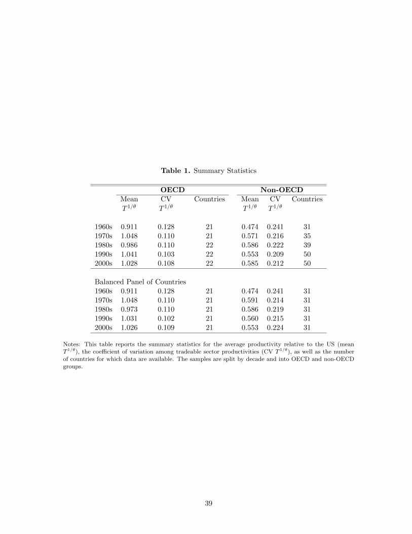
Table 1. Summary Statistics

OECD Non-OECDMean CV Countries Mean CV Countries

T 1/θ T 1/θ T 1/θ T 1/θ

1960s 0.911 0.128 21 0.474 0.241 311970s 1.048 0.110 21 0.571 0.216 351980s 0.986 0.110 22 0.586 0.222 391990s 1.041 0.103 22 0.553 0.209 502000s 1.028 0.108 22 0.585 0.212 50

Balanced Panel of Countries1960s 0.911 0.128 21 0.474 0.241 311970s 1.048 0.110 21 0.591 0.214 311980s 0.973 0.110 21 0.586 0.219 311990s 1.031 0.102 21 0.560 0.215 312000s 1.026 0.109 21 0.553 0.224 31

Notes: This table reports the summary statistics for the average productivity relative to the US (meanT 1/θ), the coefficient of variation among tradeable sector productivities (CV T 1/θ), as well as the numberof countries for which data are available. The samples are split by decade and into OECD and non-OECDgroups.

39

Tab

le2.

Pool

edR

egre

ssio

nR

esu

lts

(1)

(2)

(3)

(4)

(5)

(6)

1960

sto

2000s

198

0s

to20

00s

196

0s

to19

70s

1970s

to1980s

1980s

to1990s

1990

sto

2000

s

Dep

.V

ar:

Log

Ch

ange

inT

1/θ

Pan

elA

:A

llC

ountr

ies

Log( In

itia

lT

1/θ)

-0.5

17*

**

-0.2

08*

**-0

.228

***

-0.1

42*

**

-0.1

73***

-0.1

08***

(0.0

44)

(0.0

34)

(0.0

27)

(0.0

23)

(0.0

29)

(0.0

32)

NB

:S

peed

of

con

verg

ence

,pe

rdec

ade

0.1

82

0.1

17

0.2

59

0.1

53

0.1

90

0.1

14

Ob

serv

atio

ns

893

1,0

6895

51,

038

1,1

29

1,28

2R

20.

677

0.6

360.

722

0.65

90.6

67

0.6

84

Panel

B:

OE

CD

Log( In

itia

lT

1/θ)

-0.6

76*

**

-0.3

69*

**-0

.250

***

-0.1

76*

**

-0.2

20***

-0.1

46*

(0.0

72)

(0.0

87)

(0.0

35)

(0.0

37)

(0.0

46)

(0.0

82)

NB

:S

peed

of

con

verg

ence

,pe

rdec

ade

0.2

82

0.2

30

0.2

88

0.1

94

0.2

48

0.1

58

Ob

serv

atio

ns

393

405

396

394

407

410

R2

0.75

70.6

370.

742

0.73

40.6

54

0.5

48

Pan

elC

:n

on-O

EC

D

Log( In

itia

lT

1/θ)

-0.6

59*

**

-0.3

02*

**-0

.344

***

-0.1

91*

**

-0.2

56***

-0.1

48***

(0.0

67)

(0.0

59)

(0.0

46)

(0.0

35)

(0.0

48)

(0.0

47)

NB

:S

peed

of

con

verg

ence

,pe

rdec

ade

0.2

69

0.1

80

0.4

22

0.2

12

0.2

96

0.1

60

Ob

serv

atio

ns

500

663

559

644

722

872

R2

0.73

70.6

350.

759

0.66

20.6

21

0.7

07

Cou

ntr

yF

Eye

syes

yes

yes

yes

yes

Sec

tor

FE

yes

yes

yes

yes

yes

yes

Note

s:Sta

ndard

erro

rscl

ust

ered

at

the

countr

yle

vel

inpare

nth

eses

;***:

signifi

cant

at

1%

;*:

signifi

cant

at

10%

.T

his

table

rep

ort

sth

ere

sult

s

of

regre

ssin

gth

egro

wth

of

esti

mate

dte

chnolo

gy

para

met

er( Tj n) 1/θ

on

its

init

ial

valu

eov

erdiff

eren

tti

me

per

iods

and

subsa

mple

s.T

he

spee

dof

conver

gen

ce,

per

dec

ade,

isre

port

ed(i

nit

alics

)under

nea

thea

chco

effici

ent

esti

mate

.

40

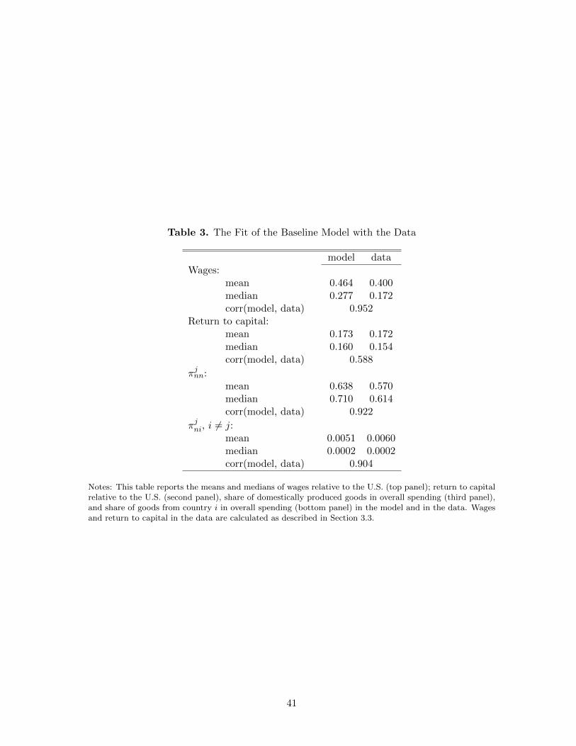
Table 3. The Fit of the Baseline Model with the Data

model dataWages:

mean 0.464 0.400median 0.277 0.172corr(model, data) 0.952

Return to capital:mean 0.173 0.172median 0.160 0.154corr(model, data) 0.588

πjnn:mean 0.638 0.570median 0.710 0.614corr(model, data) 0.922

πjni, i 6= j:mean 0.0051 0.0060median 0.0002 0.0002corr(model, data) 0.904

Notes: This table reports the means and medians of wages relative to the U.S. (top panel); return to capitalrelative to the U.S. (second panel), share of domestically produced goods in overall spending (third panel),and share of goods from country i in overall spending (bottom panel) in the model and in the data. Wagesand return to capital in the data are calculated as described in Section 3.3.

41

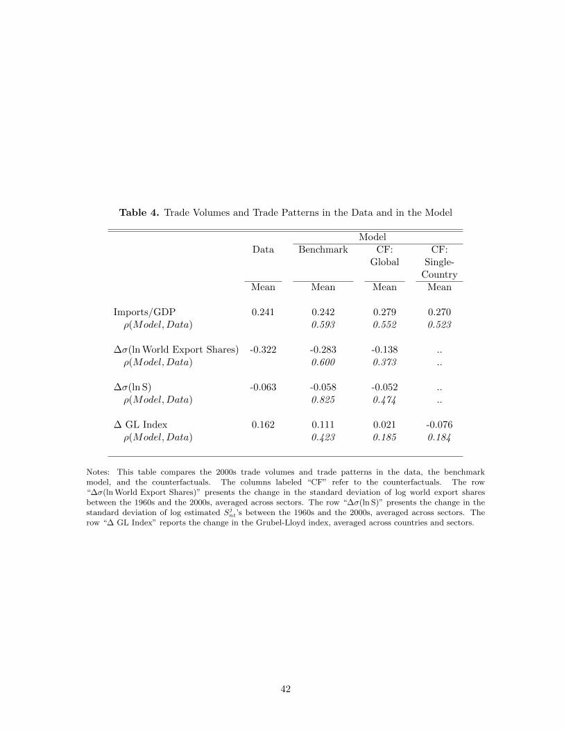
Table 4. Trade Volumes and Trade Patterns in the Data and in the Model

ModelData Benchmark CF: CF:

Global Single-Country

Mean Mean Mean Mean

Imports/GDP 0.241 0.242 0.279 0.270ρ(Model,Data) 0.593 0.552 0.523

∆σ(ln World Export Shares) -0.322 -0.283 -0.138 ..ρ(Model,Data) 0.600 0.373 ..

∆σ(ln S) -0.063 -0.058 -0.052 ..ρ(Model,Data) 0.825 0.474 ..

∆ GL Index 0.162 0.111 0.021 -0.076ρ(Model,Data) 0.423 0.185 0.184

Notes: This table compares the 2000s trade volumes and trade patterns in the data, the benchmarkmodel, and the counterfactuals. The columns labeled “CF” refer to the counterfactuals. The row“∆σ(ln World Export Shares)” presents the change in the standard deviation of log world export sharesbetween the 1960s and the 2000s, averaged across sectors. The row “∆σ(ln S)” presents the change in thestandard deviation of log estimated Sjnt’s between the 1960s and the 2000s, averaged across sectors. Therow “∆ GL Index” reports the change in the Grubel-Lloyd index, averaged across countries and sectors.

42

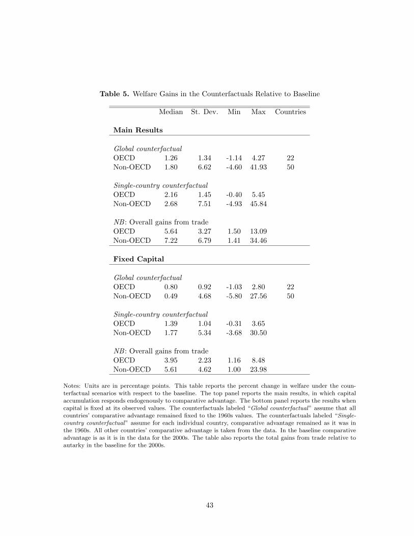
Table 5. Welfare Gains in the Counterfactuals Relative to Baseline

Median St. Dev. Min Max Countries

Main Results

Global counterfactualOECD 1.26 1.34 -1.14 4.27 22Non-OECD 1.80 6.62 -4.60 41.93 50

Single-country counterfactualOECD 2.16 1.45 -0.40 5.45Non-OECD 2.68 7.51 -4.93 45.84

NB : Overall gains from tradeOECD 5.64 3.27 1.50 13.09Non-OECD 7.22 6.79 1.41 34.46

Fixed Capital

Global counterfactualOECD 0.80 0.92 -1.03 2.80 22Non-OECD 0.49 4.68 -5.80 27.56 50

Single-country counterfactualOECD 1.39 1.04 -0.31 3.65Non-OECD 1.77 5.34 -3.68 30.50

NB : Overall gains from tradeOECD 3.95 2.23 1.16 8.48Non-OECD 5.61 4.62 1.00 23.98

Notes: Units are in percentage points. This table reports the percent change in welfare under the coun-terfactual scenarios with respect to the baseline. The top panel reports the main results, in which capitalaccumulation responds endogenously to comparative advantage. The bottom panel reports the results whencapital is fixed at its observed values. The counterfactuals labeled “Global counterfactual” assume that allcountries’ comparative advantage remained fixed to the 1960s values. The counterfactuals labeled “Single-country counterfactual” assume for each individual country, comparative advantage remained as it was inthe 1960s. All other countries’ comparative advantage is taken from the data. In the baseline comparativeadvantage is as it is in the data for the 2000s. The table also reports the total gains from trade relative toautarky in the baseline for the 2000s.

43

Fig

ure

1.

Ab

solu

tean

dR

elat

ive

Con

verg

ence

EGY

IRL

TTO

PHL

SLV

VEN

BOL

JOR

AUT

CAN

GHA

NZL

MYS

COL

IND

DNK

NLD

FIN

NOR

PRT

LKA

SWE

HND

ZAF

AUS

KENFJ

I

ISR

TUR

ISL

CRI

GBR

ITA

CHL

JPN

FRA

URY

BLX DE

U

KOR

ESP

GRC

ECU

−.20.2.4.66Ln(Average T

1/e)

−1.5

−1−.

50

Ln(In

itial A

vera

ge T

1/e )

(a)

1960s

to2000s:

Abso

lute

Conver

gen

ceand

Init

ial

Aver

-age

EGY

IRL

TTO

PHLSL

V

VEN

BOL

SEN

JOR

AUT

CAN

PER

MEX

GHA

NZL

MYS

CHE

COL

IND

DNK

NLDFI

NCH

NNO

RPR

T

LKA

SWE

HND

ETH

MUS

AUS

KEN

FJI

ISR

TUR

ISL

CRI

GBR ITA

CHL

JPN

BRA

ARG

FRA

TWN

URY

BGD

BLX DE

U

KOR

ESP

GRC

ECU ID

N

RUS

SVK

KAZ

ROM

SVN

POL

CZE

HUN

UKR

VNM

BGR

−.2−.10.1.2.36Ln(Average T

1/e)

−1.5

−1−.

50

.5Ln

(Initia

l Ave

rage

T1/e )

(b)

1990s

to2000s:

Abso

lute

Conver

gen

ceand

Init

ial

Aver

-age

EGY

IRLTT

OPH

L

SLV

VEN

BOL

JOR

AUT

CAN

GH

A

NZL

MYS

CO

LIN

D

DN

KNLD

FINN

ORPR

T

LKA

SWE

HN

D

ZAF

AUS

KEN

FJI

ISR

TUR

ISL

CR

I

GBR

ITA

CH

L

JPN

FRA

UR

Y

BLX

DEU

KOR

ESPG

RC

ECU

.05.15.25.35Coeff. Var. T

1/e, 2000s

.05

.15

.25

.35

Coe

ff. V

ar. T

1/e , 1

960s

(c)

1960s

and

2000s:

Coeffi

cien

tof

Vari

ati

on

EGY

IRL

TTOPH

L

SLV

VEN

BOL

JOR

AUT

CAN

GH

A

NZL

MYS

CO

LIN

D

DN

K

NLD

FIN

NO

R

PRT

LKA

SWE

HN

D

AUS

KEN

FJI

ISR

TUR

ISL

CR

I

GBR

ITA

CH

L

JPN

FRA

UR

Y

BLX

DEU

KOR

ESP

GR

C

ECU

.05.15.25.35Coeff. Var. T

1/e, 2000s

.05

.15

.25

.35

Coe

ff. V

ar. T

1/e , 1

990s

(d)

1990s

and

2000s:

Coeffi

cien

tof

Vari

ati

on

Note

s:T

he

top

panel

of

this

figure

pre

sents

the

biv

ari

ate

plo

tsof

abso

lute

conver

gen

cefr

om

the

1960s

(lef

tpanel

)and

the

1990s

(rig

ht

panel

)again

stlo

gin

itia

lav

erageT

1/θ

rela

tive

toth

eU

S.

The

bott

om

panel

plo

tsth

eco

effici

ent

of

vari

ati

on

inT

1/θ

rela

tive

toth

eU

Sin

the

2000s

again

stth

isva

lue

inth

e1960s

(lef

tpanel

)and

the

1990s

(rig

ht

panel

).In

the

bott

om

2panel

s,th

eline

thro

ugh

the

data

isth

e45-d

egre

eline.

44

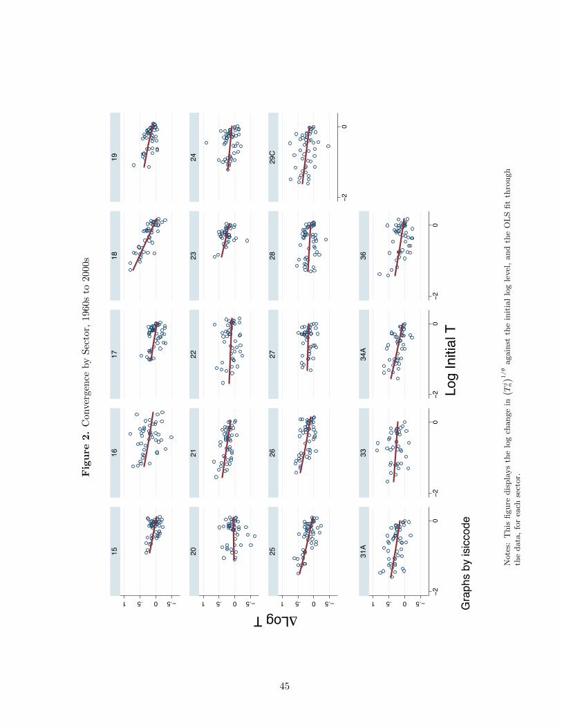
Fig

ure

2.

Con

verg

ence

by

Sec

tor,

1960

sto

2000

s

−.50.51 −.50.51 −.50.51 −.50.51

−20

−20

−20

−20

−20

1516

1718

19

2021

2223

24

2526

2728

29C

31A

3334

A36

6Log T

Log

Initi

al T

Gra

phs

by is

icco

de

Note

s:T

his

figure

dis

pla

ys

the

log

change

in( Tj n) 1/θ

again

stth

ein

itia

llo

gle

vel

,and

the

OL

Sfit

thro

ugh

the

data

,fo

rea

chse

ctor.

45

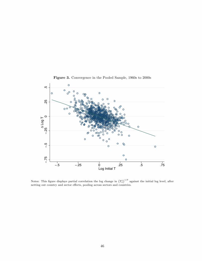
Figure 3. Convergence in the Pooled Sample, 1960s to 2000s

−.75

−.5

−.25

0.2

5.5

6 L

og T

−.5 −.25 0 .25 .5 .75Log Initial T

Notes: This figure displays partial correlation the log change in(T jn

)1/θagainst the initial log level, after

netting out country and sector effects, pooling across sectors and countries.

46

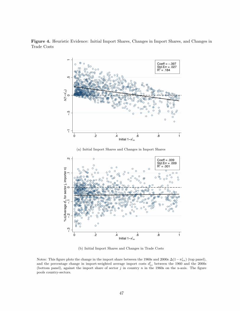
Figure 4. Heuristic Evidence: Initial Import Shares, Changes in Import Shares, and Changes inTrade Costs

Coeff = −.397Std.Err = .027R2 = .184

−1−.

50

.51

6(1−/

j nn)

0 .2 .4 .6 .8 1Initial 1−/j

nn

(a) Initial Import Shares and Changes in Import Shares

Coeff = .009Std.Err = .009R2 = .001

−.3

−.2

−.1

0.1

.2%6

(Ave

rage

dj ni

for s

ecto

r j, i

mpo

rter n

)

0 .2 .4 .6 .8 1Initial 1−/j

nn

(b) Initial Import Shares and Changes in Trade Costs

Notes: This figure plots the change in the import share between the 1960s and 2000s ∆(1−πjnn) (top panel),and the percentage change in import-weighted average import costs djni between the 1960 and the 2000s(bottom panel), against the import share of sector j in country n in the 1960s on the x-axis. The figurepools country-sectors.

47

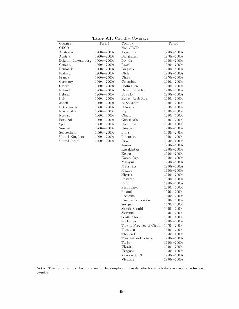
Table A1. Country CoverageCountry Period Country Period

OECD Non-OECDAustralia 1960s−2000s Argentina 1980s−2000sAustria 1960s−2000s Bangladesh 1970s−2000sBelgium-Luxembourg 1960s−2000s Bolivia 1960s−2000sCanada 1960s−2000s Brazil 1980s−2000sDenmark 1960s−2000s Bulgaria 1990s−2000sFinland 1960s−2000s Chile 1960s−2000sFrance 1960s−2000s China 1970s−2000sGermany 1960s−2000s Colombia 1960s−2000sGreece 1960s−2000s Costa Rica 1960s−2000sIceland 1960s−2000s Czech Republic 1990s−2000sIreland 1960s−2000s Ecuador 1960s−2000sItaly 1960s−2000s Egypt, Arab Rep. 1960s−2000sJapan 1960s−2000s El Salvador 1960s−2000sNetherlands 1960s−2000s Ethiopia 1980s−2000sNew Zealand 1960s−2000s Fiji 1960s−2000sNorway 1960s−2000s Ghana 1960s−2000sPortugal 1960s−2000s Guatemala 1960s−2000sSpain 1960s−2000s Honduras 1960s−2000sSweden 1960s−2000s Hungary 1990s−2000sSwitzerland 1980s−2000s India 1960s−2000sUnited Kingdom 1960s−2000s Indonesia 1960s−2000sUnited States 1960s−2000s Israel 1960s−2000s

Jordan 1960s−2000sKazakhstan 1990s−2000sKenya 1960s−2000sKorea, Rep. 1960s−2000sMalaysia 1960s−2000sMauritius 1960s−2000sMexico 1960s−2000sNigeria 1960s−2000sPakistan 1960s−2000sPeru 1980s−2000sPhilippines 1960s−2000sPoland 1990s−2000sRomania 1990s−2000sRussian Federation 1990s−2000sSenegal 1970s−2000sSlovak Republic 1990s−2000sSlovenia 1990s−2000sSouth Africa 1960s−2000sSri Lanka 1960s−2000sTaiwan Province of China 1970s−2000sTanzania 1960s−2000sThailand 1960s−2000sTrinidad and Tobago 1960s−2000sTurkey 1960s−2000sUkraine 1990s−2000sUruguay 1960s−2000sVenezuela, RB 1960s−2000sVietnam 1990s−2000s

Notes: This table reports the countries in the sample and the decades for which data are available for eachcountry.

48

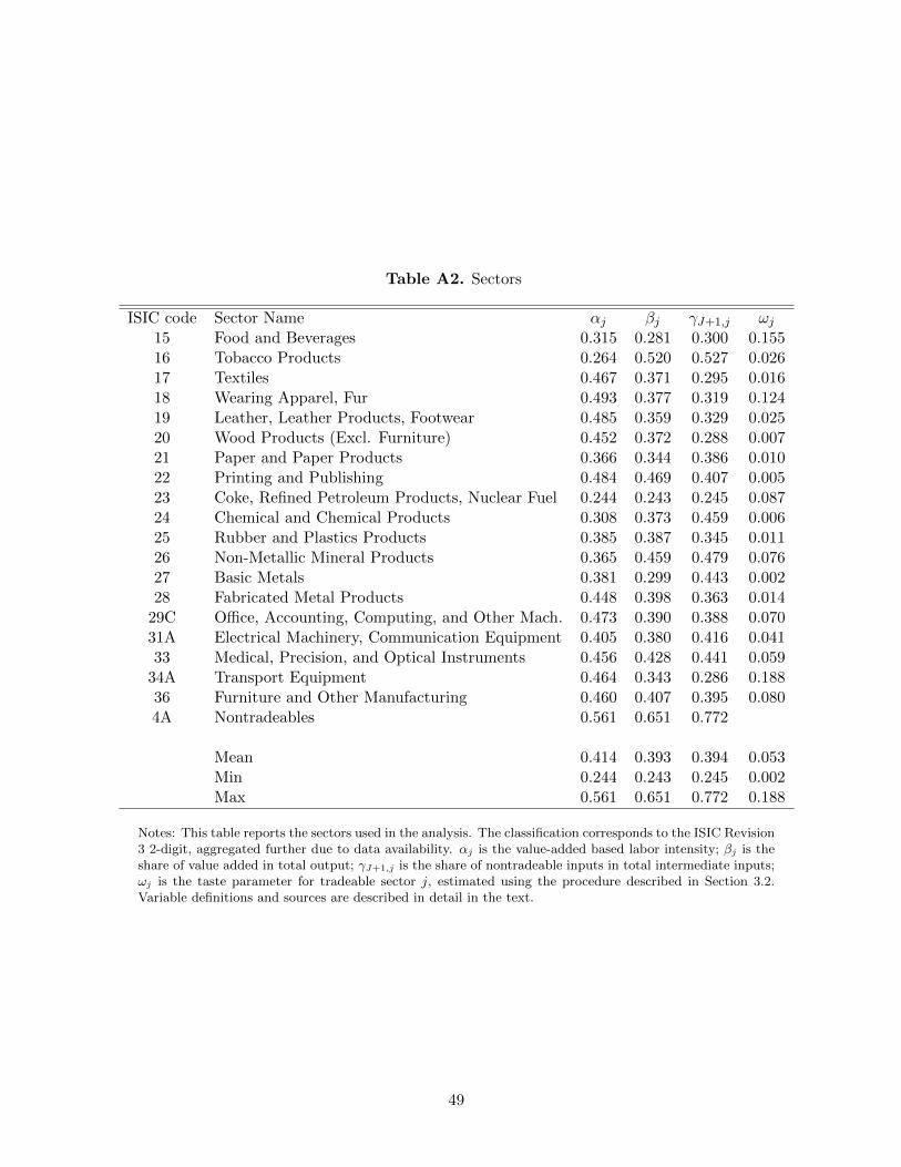
Table A2. Sectors

ISIC code Sector Name αj βj γJ+1,j ωj15 Food and Beverages 0.315 0.281 0.300 0.15516 Tobacco Products 0.264 0.520 0.527 0.02617 Textiles 0.467 0.371 0.295 0.01618 Wearing Apparel, Fur 0.493 0.377 0.319 0.12419 Leather, Leather Products, Footwear 0.485 0.359 0.329 0.02520 Wood Products (Excl. Furniture) 0.452 0.372 0.288 0.00721 Paper and Paper Products 0.366 0.344 0.386 0.01022 Printing and Publishing 0.484 0.469 0.407 0.00523 Coke, Refined Petroleum Products, Nuclear Fuel 0.244 0.243 0.245 0.08724 Chemical and Chemical Products 0.308 0.373 0.459 0.00625 Rubber and Plastics Products 0.385 0.387 0.345 0.01126 Non-Metallic Mineral Products 0.365 0.459 0.479 0.07627 Basic Metals 0.381 0.299 0.443 0.00228 Fabricated Metal Products 0.448 0.398 0.363 0.014

29C Office, Accounting, Computing, and Other Mach. 0.473 0.390 0.388 0.07031A Electrical Machinery, Communication Equipment 0.405 0.380 0.416 0.04133 Medical, Precision, and Optical Instruments 0.456 0.428 0.441 0.059

34A Transport Equipment 0.464 0.343 0.286 0.18836 Furniture and Other Manufacturing 0.460 0.407 0.395 0.0804A Nontradeables 0.561 0.651 0.772

Mean 0.414 0.393 0.394 0.053Min 0.244 0.243 0.245 0.002Max 0.561 0.651 0.772 0.188

Notes: This table reports the sectors used in the analysis. The classification corresponds to the ISIC Revision3 2-digit, aggregated further due to data availability. αj is the value-added based labor intensity; βj is theshare of value added in total output; γJ+1,j is the share of nontradeable inputs in total intermediate inputs;ωj is the taste parameter for tradeable sector j, estimated using the procedure described in Section 3.2.Variable definitions and sources are described in detail in the text.

49

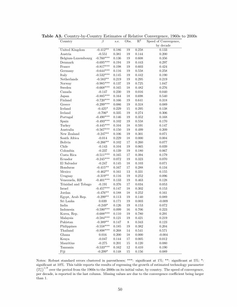
Table A3. Country-by-Country Estimates of Relative Convergence, 1960s to 2000sCountry β s.e. Obs. R2 Speed of Convergence,

by decade

United Kingdom -0.412** 0.186 19 0.258 0.133Austria -0.551 0.381 19 0.144 0.200Belgium-Luxembourg -0.760*** 0.136 19 0.608 0.356Denmark -0.695*** 0.194 19 0.443 0.297France -0.817*** 0.198 19 0.603 0.424Germany -0.644*** 0.116 19 0.558 0.258Italy -0.532*** 0.145 19 0.442 0.190Netherlands -0.583** 0.219 19 0.295 0.219Norway -0.985*** 0.137 19 0.725 1.047Sweden -0.668*** 0.165 18 0.482 0.276Canada -0.147 0.230 19 0.016 0.040Japan -0.885*** 0.164 18 0.698 0.540Finland -0.720*** 0.166 19 0.641 0.318Greece -0.299*** 0.086 19 0.318 0.089Iceland -0.425* 0.229 15 0.295 0.138Ireland -0.706* 0.335 19 0.274 0.306Portugal -0.490*** 0.146 19 0.352 0.168Spain -0.493*** 0.102 19 0.558 0.170Turkey -0.445*** 0.104 18 0.591 0.147Australia -0.567*** 0.150 19 0.499 0.209New Zealand -0.247** 0.106 19 0.301 0.071South Africa -0.014 0.229 18 0.000 0.004Bolivia -0.266** 0.102 17 0.260 0.077Chile -0.143 0.104 19 0.065 0.039Colombia -0.237 0.139 19 0.180 0.067Costa Rica -0.511*** 0.165 17 0.394 0.179Ecuador -0.245*** 0.072 19 0.323 0.070El Salvador -0.247 0.145 18 0.103 0.071Honduras -0.415** 0.167 17 0.288 0.134Mexico -0.462** 0.161 13 0.331 0.155Uruguay -0.319** 0.116 19 0.252 0.096Venezuela, RB -0.401*** 0.133 19 0.463 0.128Trinidad and Tobago -0.191 0.376 17 0.034 0.053Israel -0.457*** 0.147 18 0.302 0.153Jordan -0.476** 0.188 18 0.252 0.161Egypt, Arab Rep. -0.299** 0.113 19 0.140 0.089Sri Lanka 0.039 0.171 19 0.003 -0.009India -0.249* 0.126 19 0.153 0.072Indonesia -0.590*** 0.099 16 0.706 0.223Korea, Rep. -0.688*** 0.110 19 0.780 0.291Malaysia -0.584*** 0.121 19 0.421 0.219Pakistan -0.389** 0.147 8 0.343 0.123Philippines -0.558*** 0.185 19 0.382 0.204Thailand -0.898*** 0.268 14 0.541 0.571Ghana 0.016 0.200 18 0.000 -0.004Kenya -0.047 0.144 17 0.005 0.012Mauritius -0.275 0.201 15 0.120 0.080Tanzania -0.533*** 0.162 12 0.410 0.190Fiji -0.299* 0.148 15 0.156 0.089

Notes: Robust standard errors clustered in parentheses; ***: significant at 1%; **: significant at 5%; *:significant at 10%. This table reports the results of regressing the growth of estimated technology parameter(T jn

)1/θover the period from the 1960s to the 2000s on its initial value, by country. The speed of convergence,

per decade, is reported in the last column. Missing values are due to the convergence coefficient being largerthan 1.

50

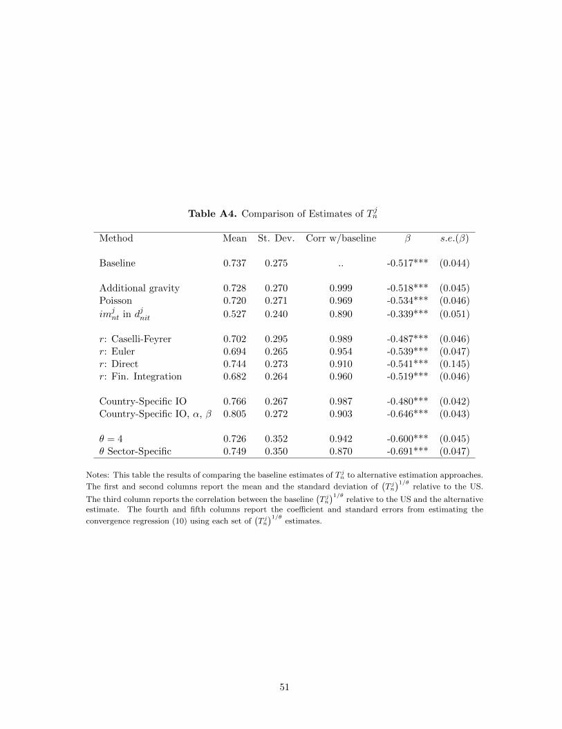
Table A4. Comparison of Estimates of T jn

Method Mean St. Dev. Corr w/baseline β s.e.(β)

Baseline 0.737 0.275 .. -0.517*** (0.044)

Additional gravity 0.728 0.270 0.999 -0.518*** (0.045)Poisson 0.720 0.271 0.969 -0.534*** (0.046)

imjnt in djnit 0.527 0.240 0.890 -0.339*** (0.051)

r: Caselli-Feyrer 0.702 0.295 0.989 -0.487*** (0.046)r: Euler 0.694 0.265 0.954 -0.539*** (0.047)r: Direct 0.744 0.273 0.910 -0.541*** (0.145)r: Fin. Integration 0.682 0.264 0.960 -0.519*** (0.046)

Country-Specific IO 0.766 0.267 0.987 -0.480*** (0.042)Country-Specific IO, α, β 0.805 0.272 0.903 -0.646*** (0.043)

θ = 4 0.726 0.352 0.942 -0.600*** (0.045)θ Sector-Specific 0.749 0.350 0.870 -0.691*** (0.047)

Notes: This table the results of comparing the baseline estimates of T jn to alternative estimation approaches.

The first and second columns report the mean and the standard deviation of(T jn

)1/θrelative to the US.

The third column reports the correlation between the baseline(T jn

)1/θrelative to the US and the alternative

estimate. The fourth and fifth columns report the coefficient and standard errors from estimating the

convergence regression (10) using each set of(T jn

)1/θestimates.

51

Table A5. Zero Trade Observations: Model vs. Data

Sector Name ISIC code 1960s 1970s 1980s 1990s 2000s

All Sectors Combined 0.007 0.006 0.006 0.001 0.009

Food and Beverages 15 0.000 0.000 0.000 0.000 0.000Tobacco Products 16 0.075 0.100 0.015 0.015 0.026Textiles 17 0.000 0.000 0.000 0.002 0.005Wearing Apparel, Fur 18 0.011 0.015 0.000 0.000 0.004Leather, Leather Products, Footwear 19 0.011 0.016 0.028 0.001 0.031Wood Products (Excl. Furniture) 20 0.001 0.000 0.000 0.000 0.013Paper and Paper Products 21 0.000 0.000 0.000 0.000 0.005Printing and Publishing 22 0.017 0.021 0.000 0.000 0.009Coke, Refined Petroleum Products, Nuclear Fuel 23 0.003 0.003 0.023 0.008 0.011Chemical and Chemical Products 24 0.000 0.000 0.000 0.000 0.004Rubber and Plastics Products 25 0.000 0.001 0.000 0.000 0.010Non-Metallic Mineral Products 26 0.000 0.000 0.000 0.000 0.001Basic Metals 27 0.003 0.001 0.000 0.000 0.011Fabricated Metal Products 28 0.000 0.000 0.036 0.000 0.020Office, Accounting, Computing, and Other Mach. 29C 0.001 0.000 0.000 0.000 0.013Electrical Machinery, Communication Equipment 31A 0.000 0.000 0.000 0.000 0.011Medical, Precision, and Optical Instruments 33 0.022 0.020 0.003 0.006 0.023Transport Equipment 34A 0.012 0.000 0.005 0.000 0.011Furniture and Other Manufacturing 36 0.012 0.015 0.005 0.002 0.012

Notes: This table reports the share of global absorption taken up by importer-exporter-sector observationsfor which actual imports are zero in the data.

52

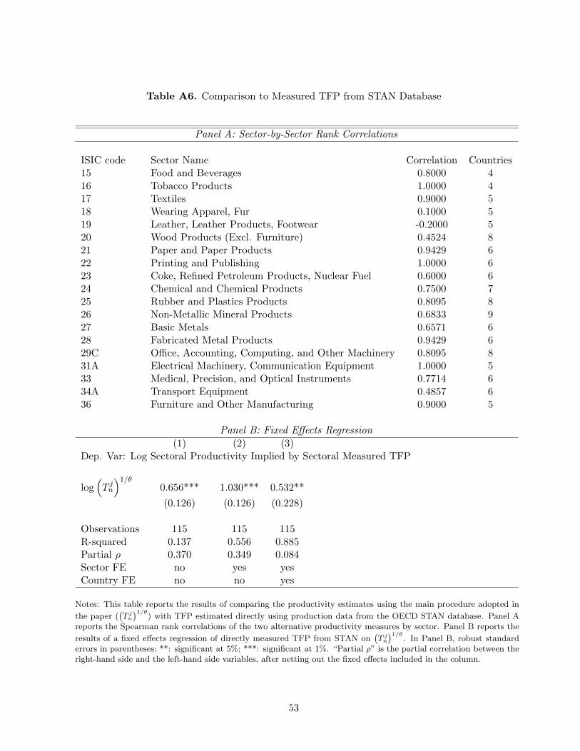
Table A6. Comparison to Measured TFP from STAN Database

Panel A: Sector-by-Sector Rank Correlations

ISIC code Sector Name Correlation Countries15 Food and Beverages 0.8000 416 Tobacco Products 1.0000 417 Textiles 0.9000 518 Wearing Apparel, Fur 0.1000 519 Leather, Leather Products, Footwear -0.2000 520 Wood Products (Excl. Furniture) 0.4524 821 Paper and Paper Products 0.9429 622 Printing and Publishing 1.0000 623 Coke, Refined Petroleum Products, Nuclear Fuel 0.6000 624 Chemical and Chemical Products 0.7500 725 Rubber and Plastics Products 0.8095 826 Non-Metallic Mineral Products 0.6833 927 Basic Metals 0.6571 628 Fabricated Metal Products 0.9429 629C Office, Accounting, Computing, and Other Machinery 0.8095 831A Electrical Machinery, Communication Equipment 1.0000 533 Medical, Precision, and Optical Instruments 0.7714 634A Transport Equipment 0.4857 636 Furniture and Other Manufacturing 0.9000 5

Panel B: Fixed Effects Regression

(1) (2) (3)Dep. Var: Log Sectoral Productivity Implied by Sectoral Measured TFP

log(T jn)1/θ

0.656*** 1.030*** 0.532**

(0.126) (0.126) (0.228)

Observations 115 115 115R-squared 0.137 0.556 0.885Partial ρ 0.370 0.349 0.084Sector FE no yes yesCountry FE no no yes

Notes: This table reports the results of comparing the productivity estimates using the main procedure adopted in

the paper ((T jn

)1/θ) with TFP estimated directly using production data from the OECD STAN database. Panel A

reports the Spearman rank correlations of the two alternative productivity measures by sector. Panel B reports the

results of a fixed effects regression of directly measured TFP from STAN on(T jn

)1/θ. In Panel B, robust standard

errors in parentheses; **: significant at 5%; ***: significant at 1%. “Partial ρ” is the partial correlation between theright-hand side and the left-hand side variables, after netting out the fixed effects included in the column.

53

1

Working Paper Series

A series of research studies on regional economic issues relating to the Seventh Federal Reserve District, and on financial and economic topics.

Corporate Average Fuel Economy Standards and the Market for New Vehicles WP-11-01 Thomas Klier and Joshua Linn The Role of Securitization in Mortgage Renegotiation WP-11-02 Sumit Agarwal, Gene Amromin, Itzhak Ben-David, Souphala Chomsisengphet, and Douglas D. Evanoff Market-Based Loss Mitigation Practices for Troubled Mortgages Following the Financial Crisis WP-11-03 Sumit Agarwal, Gene Amromin, Itzhak Ben-David, Souphala Chomsisengphet, and Douglas D. Evanoff Federal Reserve Policies and Financial Market Conditions During the Crisis WP-11-04 Scott A. Brave and Hesna Genay The Financial Labor Supply Accelerator WP-11-05 Jeffrey R. Campbell and Zvi Hercowitz Survival and long-run dynamics with heterogeneous beliefs under recursive preferences WP-11-06 Jaroslav Borovička A Leverage-based Model of Speculative Bubbles (Revised) WP-11-07 Gadi Barlevy Estimation of Panel Data Regression Models with Two-Sided Censoring or Truncation WP-11-08 Sule Alan, Bo E. Honoré, Luojia Hu, and Søren Leth–Petersen Fertility Transitions Along the Extensive and Intensive Margins WP-11-09 Daniel Aaronson, Fabian Lange, and Bhashkar Mazumder Black-White Differences in Intergenerational Economic Mobility in the US WP-11-10 Bhashkar Mazumder Can Standard Preferences Explain the Prices of Out-of-the-Money S&P 500 Put Options? WP-11-11 Luca Benzoni, Pierre Collin-Dufresne, and Robert S. Goldstein Business Networks, Production Chains, and Productivity: A Theory of Input-Output Architecture WP-11-12 Ezra Oberfield Equilibrium Bank Runs Revisited WP-11-13 Ed Nosal Are Covered Bonds a Substitute for Mortgage-Backed Securities? WP-11-14 Santiago Carbó-Valverde, Richard J. Rosen, and Francisco Rodríguez-Fernández The Cost of Banking Panics in an Age before “Too Big to Fail” WP-11-15 Benjamin Chabot

2

Working Paper Series (continued) Import Protection, Business Cycles, and Exchange Rates: Evidence from the Great Recession WP-11-16 Chad P. Bown and Meredith A. Crowley Examining Macroeconomic Models through the Lens of Asset Pricing WP-12-01 Jaroslav Borovička and Lars Peter Hansen The Chicago Fed DSGE Model WP-12-02 Scott A. Brave, Jeffrey R. Campbell, Jonas D.M. Fisher, and Alejandro Justiniano Macroeconomic Effects of Federal Reserve Forward Guidance WP-12-03 Jeffrey R. Campbell, Charles L. Evans, Jonas D.M. Fisher, and Alejandro Justiniano Modeling Credit Contagion via the Updating of Fragile Beliefs WP-12-04 Luca Benzoni, Pierre Collin-Dufresne, Robert S. Goldstein, and Jean Helwege Signaling Effects of Monetary Policy WP-12-05 Leonardo Melosi Empirical Research on Sovereign Debt and Default WP-12-06 Michael Tomz and Mark L. J. Wright Credit Risk and Disaster Risk WP-12-07 François Gourio From the Horse’s Mouth: How do Investor Expectations of Risk and Return Vary with Economic Conditions? WP-12-08 Gene Amromin and Steven A. Sharpe Using Vehicle Taxes To Reduce Carbon Dioxide Emissions Rates of New Passenger Vehicles: Evidence from France, Germany, and Sweden WP-12-09 Thomas Klier and Joshua Linn Spending Responses to State Sales Tax Holidays WP-12-10 Sumit Agarwal and Leslie McGranahan Micro Data and Macro Technology WP-12-11 Ezra Oberfield and Devesh Raval The Effect of Disability Insurance Receipt on Labor Supply: A Dynamic Analysis WP-12-12 Eric French and Jae Song Medicaid Insurance in Old Age WP-12-13 Mariacristina De Nardi, Eric French, and John Bailey Jones Fetal Origins and Parental Responses WP-12-14 Douglas Almond and Bhashkar Mazumder

3

Working Paper Series (continued) Repos, Fire Sales, and Bankruptcy Policy WP-12-15 Gaetano Antinolfi, Francesca Carapella, Charles Kahn, Antoine Martin, David Mills, and Ed Nosal Speculative Runs on Interest Rate Pegs The Frictionless Case WP-12-16 Marco Bassetto and Christopher Phelan Institutions, the Cost of Capital, and Long-Run Economic Growth: Evidence from the 19th Century Capital Market WP-12-17 Ron Alquist and Ben Chabot Emerging Economies, Trade Policy, and Macroeconomic Shocks WP-12-18 Chad P. Bown and Meredith A. Crowley The Urban Density Premium across Establishments WP-13-01 R. Jason Faberman and Matthew Freedman Why Do Borrowers Make Mortgage Refinancing Mistakes? WP-13-02 Sumit Agarwal, Richard J. Rosen, and Vincent Yao Bank Panics, Government Guarantees, and the Long-Run Size of the Financial Sector: Evidence from Free-Banking America WP-13-03 Benjamin Chabot and Charles C. Moul Fiscal Consequences of Paying Interest on Reserves WP-13-04 Marco Bassetto and Todd Messer Properties of the Vacancy Statistic in the Discrete Circle Covering Problem WP-13-05 Gadi Barlevy and H. N. Nagaraja Credit Crunches and Credit Allocation in a Model of Entrepreneurship WP-13-06 Marco Bassetto, Marco Cagetti, and Mariacristina De Nardi Financial Incentives and Educational Investment: The Impact of Performance-Based Scholarships on Student Time Use WP-13-07 Lisa Barrow and Cecilia Elena Rouse The Global Welfare Impact of China: Trade Integration and Technological Change WP-13-08 Julian di Giovanni, Andrei A. Levchenko, and Jing Zhang Structural Change in an Open Economy WP-13-09 Timothy Uy, Kei-Mu Yi, and Jing Zhang The Global Labor Market Impact of Emerging Giants: a Quantitative Assessment WP-13-10 Andrei A. Levchenko and Jing Zhang

4

Working Paper Series (continued) Size-Dependent Regulations, Firm Size Distribution, and Reallocation WP-13-11 François Gourio and Nicolas Roys Modeling the Evolution of Expectations and Uncertainty in General Equilibrium WP-13-12 Francesco Bianchi and Leonardo Melosi Rushing into American Dream? House Prices, Timing of Homeownership, and Adjustment of Consumer Credit WP-13-13 Sumit Agarwal, Luojia Hu, and Xing Huang The Earned Income Tax Credit and Food Consumption Patterns WP-13-14 Leslie McGranahan and Diane W. Schanzenbach Agglomeration in the European automobile supplier industry WP-13-15 Thomas Klier and Dan McMillen Human Capital and Long-Run Labor Income Risk WP-13-16 Luca Benzoni and Olena Chyruk The Effects of the Saving and Banking Glut on the U.S. Economy WP-13-17 Alejandro Justiniano, Giorgio E. Primiceri, and Andrea Tambalotti A Portfolio-Balance Approach to the Nominal Term Structure WP-13-18 Thomas B. King Gross Migration, Housing and Urban Population Dynamics WP-13-19 Morris A. Davis, Jonas D.M. Fisher, and Marcelo Veracierto Very Simple Markov-Perfect Industry Dynamics WP-13-20 Jaap H. Abbring, Jeffrey R. Campbell, Jan Tilly, and Nan Yang Bubbles and Leverage: A Simple and Unified Approach WP-13-21 Robert Barsky and Theodore Bogusz The scarcity value of Treasury collateral: Repo market effects of security-specific supply and demand factors WP-13-22 Stefania D'Amico, Roger Fan, and Yuriy Kitsul Gambling for Dollars: Strategic Hedge Fund Manager Investment WP-13-23 Dan Bernhardt and Ed Nosal Cash-in-the-Market Pricing in a Model with Money and Over-the-Counter Financial Markets WP-13-24 Fabrizio Mattesini and Ed Nosal An Interview with Neil Wallace WP-13-25 David Altig and Ed Nosal

5

Working Paper Series (continued) Firm Dynamics and the Minimum Wage: A Putty-Clay Approach WP-13-26 Daniel Aaronson, Eric French, and Isaac Sorkin Policy Intervention in Debt Renegotiation: Evidence from the Home Affordable Modification Program WP-13-27 Sumit Agarwal, Gene Amromin, Itzhak Ben-David, Souphala Chomsisengphet, Tomasz Piskorski, and Amit Seru The Effects of the Massachusetts Health Reform on Financial Distress WP-14-01 Bhashkar Mazumder and Sarah Miller Can Intangible Capital Explain Cyclical Movements in the Labor Wedge? WP-14-02 François Gourio and Leena Rudanko Early Public Banks WP-14-03 William Roberds and François R. Velde Mandatory Disclosure and Financial Contagion WP-14-04 Fernando Alvarez and Gadi Barlevy The Stock of External Sovereign Debt: Can We Take the Data at ‘Face Value’? WP-14-05 Daniel A. Dias, Christine Richmond, and Mark L. J. Wright Interpreting the Pari Passu Clause in Sovereign Bond Contracts: It’s All Hebrew (and Aramaic) to Me WP-14-06 Mark L. J. Wright AIG in Hindsight WP-14-07 Robert McDonald and Anna Paulson On the Structural Interpretation of the Smets-Wouters “Risk Premium” Shock WP-14-08 Jonas D.M. Fisher Human Capital Risk, Contract Enforcement, and the Macroeconomy WP-14-09 Tom Krebs, Moritz Kuhn, and Mark L. J. Wright Adverse Selection, Risk Sharing and Business Cycles WP-14-10 Marcelo Veracierto Core and ‘Crust’: Consumer Prices and the Term Structure of Interest Rates WP-14-11 Andrea Ajello, Luca Benzoni, and Olena Chyruk

The Evolution of Comparative Advantage: Measurement and Implications WP-14-12 Andrei A. Levchenko and Jing Zhang