the evolution of combinatorial phonology · the evolution of combinatorial phonology willem zuidema...
TRANSCRIPT

The Evolution of Combinatorial Phonology
Willem ZuidemaInstitute for Logic, Language and Computation, University of Amsterdam
Plantage Muidergracht 241018 TV Amsterdam
Bart de BoerArtificial Intelligence, University of Groningen
Grote Kruisstraat 2/19712 TS GroningenThe Netherlands
January 9, 2006
Abstract
A fundamental, universal property of human language is that its phonology is combinato-rial. That is, one can identify a set of basic, distinct units (phonemes, syllables) that can beproductively combined in many different ways. In this paper, we review a number of theoriesand models that have been developed to explain the evolutionary transition from holisticto combinatorial signal systems, but find that in all problematic linguistic assumptions aremade, or crucial components of evolutionary explanations are omitted. We present a novelmodel to investigate the hypothesis that combinatorial phonology results from optimisingsignal systems for perceptual distinctiveness. Our model differs from previous models intwo important respects. First, signals are modelled as trajectories through acoustic space.Hence, both holistic and combinatorial signals have a temporal structure. Second, we usethe methodology from evolutionary game theory. Crucially, we show a path of ever in-creasing fitness from holistic to combinatorial signals, where every innovation represents anadvantage even if no-one else in a population has yet obtained it.
1 Introduction
1.1 Natural language phonology is combinatorial
One of the universal properties of human language is that its phonology is combinatorial. In
all human languages, utterances can be split into units that can be recombined into new valid
utterances. Although there is some controversy about what exactly the units of (productive)
combination are, there is general agreement that in natural languages – including even sign
languages (Deuchar, 1996) – meaningless atomic units (phonemes or syllables) are combined
into larger wholes; these meaningful combinations (words, or morphemes) are then further
1

combined into meaningful sentences. These two levels of combination constitute the duality of
patterning (Hockett, 1960).
In the traditional view, the atomic units are phonemes (minimal speech sounds that can
make a distinction in meaning), or the distinctive features of these phonemes (Chomsky and
Halle, 1968). Signal repertoires that are built-up from combinations of phonemes are said to
be “phonemically coded” (Lindblom et al., 1984). For instance, the words “we”, “me”, “why”
and “my”, as pronounced in standard British English, can be analysed as built-up from the
units “w”, “m”, “e” and “y”, which can all be used in many different combinations. One
popular alternative view is that the atoms are syllables, or the possible onsets, codas and nuclei
of syllables (e.g. Levelt and Wheeldon, 1994). A second alternative theory uses exemplars,
which can comprise several syllables or even words, as its basic units (e.g. Pierrehumbert,
2001). In this paper we will avoid the debate about the exact level of combination – and
the conventional term “phonemic coding” – and instead focus on the uncontroversial abstract
property of “combinatorial phonology”1.
Note that, whichever the real level of combination is, there is no logical necessity to assume
that all recurring sound patterns observed in speech, are in fact units of productive combination
in the speaker’s brain. For instance, if one accepts that syllables or exemplars are the units of
combination used by the speaker, phonemes are still a useful level of description to characterise
differences in meaning. We distinguish between:
1. productively combinatorial phonology, where the cognitive mechanisms for producing,
recognising and remembering signals make use of a limited sets of units that are com-
bined in many different combinations. Productive combinatoriality is a property of the
internal representations of language in the speaker (I-language).
2. superficially combinatorial phonology, where parts of signals overlap with parts of other
signals. Superficial combinatoriality is a property of the observable language (E-language).
Importantly, the overlapping parts of different signals need not necessarily also be the units
of combination of the underlying linguistic representations.
This paper is concerned with mathematical and computational theories of the evolution
of combinatoriality of human languages at both these levels. It has often been observed that
natural language phonology is discrete, in that it allows only a small number of basic sounds and
not all feasible sounds in between. In this paper we argue that it is important to distinguish
between discreteness per se, and superficial and productive combinatoriality. In section 2,
we will review existing models of Liljencrants and Lindblom (1972), Lindblom et al. (1984),
1In the animal behaviour literature the term “phonological syntax” (coined by Peter Marler, see Ujhelyi, 1996)is often used, and Michael Studdert-Kennedy also uses the term “particulate principle” (coined by W. Abler, seeStuddert-Kennedy, 1998). Jackendoff (2002, p.238) uses the term “combinatorial, phonological system” on whichour terminology is based.
2

de Boer (2001) and Oudeyer (2001, 2002, 2005), and argue that they are relevant for the
origins of discreteness, but have little to say about the origins of superficial and combinatorial
phonology. Nowak and Krakauer (1999) and Nowak et al. (1999) do address the origins of
productive combinatoriality, but these models have a number of shortcomings that make them
unconvincing as an explanation for its evolution.
In our own model, that we will introduce in section 3, we address the questions of why
natural language phonology is both discrete and superficially combinatorial. We assume, but
do not show in this paper, that superficial combinatoriality is an important intermediate stage
in the evolution of productive combinatoriality.
1.2 The origins of combinatorial phonology
Although discrete, combinatorial phonology has often been described as a uniquely human trait
(e.g. Hockett, 1960; Jackendoff, 2002), it is increasingly realised that many examples of bird and
cetacean songs (e.g. Doupe and Kuhl, 1999; Payne and McVay, 1971) and, importantly, non-
human primate calls are combinatorial as well (Ujhelyi, 1996). For instance, the “long calls”
of tamarin monkeys are built up from many repetitions of the same element (e.g. Masataka,
1987), and those of gibbons (e.g. Mitani and Marler, 1989) and chimpanzees (e.g. Arcadi, 1996)
of elaborate combinations of a repertoire of notes.
Such comparative data should be taken seriously, but it is unwarranted to view combinatorial
long calls in other primates as an immediate precursor of human combinatorial phonology,
because there are some important qualitative differences:
• Although a number of building blocks might be used repeatedly to construct a call, it
does not appear to be the case that rearranging the building blocks results in a call with
a different meaning.
• It is unclear to what extent the building blocks of primate “long calls” are flexible and
whether they are learnt.
• In human language, combinatorial phonology functions as one half of the “duality of pat-
terning”: together with recursive, compositional semantics it yields the unlimited produc-
tivity of natural language, but it is unclear if the single combinatorial system of primates
can be seen as its precursor.
Nevertheless, combinatorial phonology must have evolved from holistic systems by natural
selection. There are at least two views on what the advantages of combinatorial coding over
holistic coding are:
1. It makes it possible to transmit a larger number of messages over a noisy channel (the
“noise robustness argument”, an argument from information theory, e.g. Nowak and
3

Krakauer, 1999). Note that this argument requires that the basic elements are distinct
from each other, and that signals are strings of these basic elements. The argument does
not address, however, how signals are stored and created;
2. It makes it possible to create an infinitely extensible set of signals with a limited number
of building blocks. Such productivity provides a solution for memory limitations, because
signals can be encoded more efficiently, and for generalisation, because new signals can
be created by combining existing building blocks (the “productivity argument”, a point
often made in the generative linguistics tradition, e.g. Jackendoff, 2002). Note that this
argument deals purely with the cognitive aspects, and views the acoustic result more as
a side-effect.
These views are a good starting point for investigating the question of why initially holistic
systems (which seem to be the default for smaller repertoires of calls) would evolve toward
combinatorial systems. However, just showing an advantage does not constitute an evolutionary
explanation (Parker and Maynard Smith, 1990). At the very least, evolutionary explanations
of an observed phenotype, involve a characterisation of (i) the set of possible phenotypes, (ii)
the fitness function over those phenotypes, and (iii) a sequence of intermediate steps from an
hypothesised initial state to observed phenotype. For each next step, one needs to establish that
(iv) it has selective advantage over the previous, and thus can invade in a population without
it. In section 2 we will criticise some existing models because they lack some of these required
components.
In language evolution, fitness will not be a function of the focal individual’s traits alone,
but also of those of its conversation partners. That is, the selective advantage of a linguistic
trait will depend on the frequency of that trait and other traits in a population (it is “frequency
dependent”). Therefore, evolutionary game-theory (Maynard Smith, 1982) is the appropriate
framework for formalising evolutionary explanations for language (Nowak and Krakauer, 1999;
Komarova and Nowak, 2003; Smith, 2004; van Rooij, 2004; Jager, 2005). In this framework,
the crucial concept is that of an evolutionary stable strategy (henceforth, ESS): a strategy that
cannot be invaded by any other strategy (Maynard Smith and Price, 1973). Thus formulated,
the challenge is to show that (i) repertoires of signals with a combinatorial phonology are
ESSs, and that (ii) plausible precursor repertoires, without combinatorial phonology, are not
evolutionarily stable.
There are also theories of the origins of combinatorial phonology that do not assume a role
for natural selection. For instance, Lindblom et al. (1984), de Boer (2001) and Oudeyer (2001,
2002) see “self-organisation” as the mechanism responsible for the emergence of combinatorial
phonology. These authors use the term self-organisation in a very broad sense, where it can
refer to almost any process of pattern formation other than classical, Darwinian evolution.
4

Liljencrants and Lindblom (1972) use an optimisation heuristic, but do not make explicit which
process underlies the optimisation. In the next section we will argue that self-organisation and
natural selection need not be put in opposition, but can be seen as detailing proximate and
ultimate causes respectively (Tinbergen, 1963; Hauser, 1996), where natural selection modifies
the parameters of a self-organising process (Waddington, 1939; Boerlijst and Hogeweg, 1991).
2 Existing Approaches
2.1 Maximising discriminability
Liljencrants and Lindblom (1972) argued that one can understand the structure of the sound
systems in natural language as determined by physical factors, such as perceptual discriminabil-
ity and articulatory ease, and not as the result of arbitrary settings of abstract parameters (as in
the theories from the generative phonology tradition, e.g. Chomsky and Halle, 1968). In their
paper they focused on the discriminability of vowel repertoires, and proposed the following
metric to measure their quality:
E =1
2
∑
i,j 6=i∈R
1
d2ij
=
|R|∑
i=2
i−1∑
j=1
1
d2ij
(1)
where R is a repertoire with |R| distinct sounds, and dij is the perceptual distance between
sound i and sound j. The perceptual distance between vowels is determined by the position
of peaks (resonances) in the vowel’s frequency spectrum. The frequency of the first and the
second peak can be used as coordinates in a two-dimensional space. The weighted Euclidean
distance between two such points turns out to be a good measure of perceptual distance between
vowels. E is a measure for the quality of the system, where lower values correspond to a better
distinguishable repertoire. The E stands for “energy”, in analogy with the potential energy
that is minimised in various models in physics.
Lindblom & Liljencrants performed computer simulations using a simple hill-climbing heuris-
tic, where at each step a random change to the repertoire is considered, and adopted only if it
has a lower energy than the current state. Their results compared favourably to observed data
on vowel system distributions. These results were important because they showed that sound
systems in natural languages are not arbitrary. Rather, they can be understood as the result
of more fundamental principles. However, a number of questions remain. First of all, what in
the real world exactly is the optimisation criterion meant to be modelling? It is important to
realise that the optimisation criterion in equation (1) is neither maximising the distances be-
tween vowels nor minimising the probability of confusion. Minimising E = 12
∑
i,j 6=i∈R 1/d2ij by
changing the configuration of a set of vowels in a restricted acoustic space, is not necessarily the
same a maximising the average distance d = 1N
∑
i,j 6=i∈R dij (or squared distance), nor is it the
same as minimising the average confusion probability C = 1N
∑Ni,j 6=i∈R P (j perceived |i uttered ).
5

At intermediate distances, these three criteria behave very similarly. The crucial difference is
at distance 0, where Lindblom & Liljencrants’s E goes to infinity, and at large distances, when
both the E and C measure, but not d, approach 0. In section 3.2 we will argue that Liljen-
crants and Lindblom’s E behaves unrealistically, and that minimising the average confusion
probability (or equivalently, maximising the distinctiveness D = 1 − C) is a better criterion.
Second, we should ask which mechanism in the real world is responsible for the optimisation.
Lindblom himself has referred to both natural selection and self-organisation. The frequency
dependence of language evolution makes that natural selection at the level of the individual
cannot be equated with optimisation at the level of the population (see Zuidema and de Boer,
2003). Before we can invoke natural selection, we need to do at least a game-theoretic analysis
to show that every new configuration of signals in the acoustic space can invade in a population
where it is extremely rare. We call this the “invasibility constraint”. Models of this type will be
discussed in the next section. For self-organisation, the mechanism for optimisation has been
worked out more precisely. De Boer (2000; 2001) has studied a simulation model of a population
of individuals that each strive to imitate the vowels of others, and be imitated successfully by
others. He showed that in a process of self-organisation, similar configurations of vowels emerge
as in the Lindblom & Liljencrants model, and as found empirically in the languages of the world.
Finally, the important question remains of how to extend these models to more complex
signals. The models of Lindblom, Liljencrants and de Boer only deal with vowels and, hence,
only with the discrete aspect of human phonology. They have little to say about the evolution
of superficial and productive combination. Lindblom et al. (1984), and similarly de Boer (1999,
chapter 7), have studied models where signals are trajectories, going from a point in a consonant
space, to a point in a vowel space. But in these models the issue is still really the emergence
of categories, because the sequencing of sounds is taken as given. In this paper, in contrast, we
will focus on the emergence of superficial combination.
2.2 Natural selection for combinatorial phonology
Nowak and Krakauer (1999) apply notions from information theory and evolutionary game
theory to the evolution of language. They derive an expression for the “fitness of a language”.
Imagine a population of individuals, a set of possible signals and a set of possible meanings
to communicate about. Speakers choose a meaning to express (the intention), and choose a
signal for it with a certain probability. Hearers receive the signal, possibly distorted due to a
certain degree of noise. Hearers subsequently decode the (distorted) signal and arrive at an
interpretation.
Nowak & Krakauer observe that when communication is noisy and when a unique signal
is used for every meaning, the fitness is limited by an “error limit”: only a limited number of
sounds can be used — and thus a limited number of meanings be expressed — because by using
6

more sounds the successful recognition of the current signals would be impeded. They further
show that in such noisy conditions, fitness is higher when (meaningless) sounds are combined
into longer words. These results are essentially instantiations of Shannon’s more general results
on “noisy coding” (Shannon, 1948), as is explored in a later paper by the same group (Plotkin
and Nowak, 2000).
More interesting is the question how natural selection could favour a linguistic innovation
in a population where that innovation is still very rare. Nowak and Krakauer (1999) do not
address that specific problem mathematically. They do, however, perform a mathematical,
game-theoretic analysis of the evolution of “compositionality”, and point out that this analysis
can be adapted easily to the case of combinatorial phonology, as is worked out in Zuidema (2005).
In such an analysis, all mixed strategies are considered where both holistic and combinatorial
signals are used.
Nowak & Krakauer assume that the confusion between holistic signals is larger than the
confusion between combinatorial signals, and that there is no confusion between the two types
of strategies. From these assumptions it follows that a more combinatorial language can always
invade a population with a less combinatorial language. This is the case, because for languages
L and L′ (with proportions of combinatorial signals x and x′, respectively) it turns out that:
F (L′, L′) > F (L,L′) > F (L,L) if x′ > x. (2)
where F (a, b) is the expected communicative success (fitness) of users of language a communi-
cating with users of language b.
If L′ is very infrequent, then all speakers of language L (the “residents”) will have a fitness of
approximately F (L,L) and the rare speakers of language L′ (the “mutants”) will have fitness of
approximately F (L,L′), because for both residents and mutants the vast majority of interactions
will be with speakers of language L. Once the frequency of mutants starts to rise, the residents
will gain in fitness, that is, move toward a fitness F (L,L′). However, the mutants will gain even
more by interacting more and more with other mutants, that is, move toward F (L ′, L′). Hence,
these calculations show that strategies that use more combinatoriality can invade strategies
that use less. This means that the evolutionary dynamics of languages under natural selection
should lead to compositionality and combinatorial phonology.
Although this model is a useful formalisation of the problem and gives some important
insights, as an explanation for the evolution of combinatorial phonology (and compositionality)
it is unconvincing. The problem is that the model only considers the advantages of combinatorial
strategies, and ignores two obvious disadvantages: (1) by having a “mixed strategy” individuals
have essentially two languages in parallel, which one should expect to be costly because of
memory and learning demands and additional confusion. Nowak & Krakauer simply assume
that the second system is in place, and that the hearer interprets all signals correctly, even
7

if x is close to 0, and the number of learning experiences is therefore extremely small; (2)
combinatorial signals that consist of two or more sounds take longer to utter and are thus more
costly2. A fairer comparison would be between holistic signals of a certain duration (where
continuation of the same sound decreases the effect of noise) and combinatorial signals of the
same duration (where the digital coding decreases the effect of noise). This is the approach
we take in the model of this paper, but like Nowak & Krakauer, we will look at invasibility in
addition to optimisation.
2.3 Crystallisation in the perception–imitation cycle
A completely different approach to combinatorial phonology is based on “categorical percep-
tion”. Categorical perception (Harnad, 1987) is the phenomenon that categorisation influences
the perception of stimuli in such a way that differences between categories are perceived as
larger and differences within categories as smaller than they really are (according to an “ob-
jective”, cross-linguistic similarity metric). For instance, infants of six months old are already
unable to perceive distinctions between sounds that are not phonemes in their native language,
something they were able to do at birth (Kuhl et al., 1992). Hence, when presented syllables as
stimuli ranging from /ba/ to /pa/ in fixed increments, British subjects will hear the first stimuli
as ba’s, and the last as pa’s, without perceiving an intermediate signal (Cooper et al., 1952).
Apparently, the frequency and position of acoustic stimuli gives rise to particular phoneme
prototypes, and the prototypes in turn “warp” the perception.
Oudeyer (2001, 2002) observes that signals survive from generation to generation because
they are perceived and imitated. Because of categorical perception, the imitation will not always
be exactly the same as the perceived signal. However, the signals that are produced shape the
categories of the next generation. Thus there is feedback between emitted signals, formation
of categories and perception. This shapes the repertoire of signals in a cycle from articulation
to perception to articulation (the perception–imitation cycle; see also Westermann, 2001 and
Westermann and Miranda, 2004, for models of sensory-motor integration and their relevance
for imitation and categorical perception).
Oudeyer (2001) presents a model to study this phenomenon. In this model, signals are
modelled as points in an acoustic space. The model consists of two coupled neural maps, one
for perception and one for articulation. The perceptual map is of a type known to be able
to model categorical perception: its categorisation behaviour changes in response to the input
data. In addition, the associations between perceptual stimuli and articulatory commands are
learnt. Through this coupling between perceptual and articulatory maps, a positive feedback
2It is, of course, slightly awkward to criticise a model that Nowak and Krakauer (1999) never actually workedout. The point here is that if one takes all the assumptions that they do spell out in the paper, and work out themodel as they suggest, the result is unsatisfactory. A better model of the evolution of combinatorial phonologymust start with different assumptions.
8

loop emerges where slight non-uniformities in the input data lead to clusters in the perceptual
map, as well as weak clusters in the articulatory map, and hence to slightly stronger non-
uniformities in the distribution of acoustic signals. Oudeyer calls the collapse of signals into a
small number of clusters “crystallisation”.
Oudeyer (2002) generalises these results to a model with (quasi-) continuous trajectories,
where a production module triggers a sequence of targets in the articulatory map, which yield
a continuous trajectory. Also in this version of the model, well-defined clusters form in the
perceptual and articulatory maps. The signals can thus be analysed as consisting of sequences
of phonemes.
Oudeyer’s model is fascinating, because it gives a completely non-adaptive mechanism for the
emergence of combinatorial phonology. However, the question whether recombination increases
the functionality of the language, and thus the fitness of the individual that uses it, remains
unanswered. If it is not functional, one would expect selection to work against it. In particular,
in Oudeyer’s first model (2001), where signals are instantaneous, a large repertoire of signals
collapses into a small number of clusters. A functional pressure to maintain the number of
distinct signals would thus have to either reverse the crystallisation, or combine signals from
different clusters.
In his second model (Oudeyer, 2002), signals are continuous trajectories and potentially a
much larger distinct repertoire can emerge. However, the functionality of the repertoire is not
monitored, and plays no role in the dynamics. It might or might not be sufficient. The number
of “phonemes” (the discrete aspect) that forms is a consequence of the parameters and initial
configuration, and in a sense accidental. The reuse (the superficial combination aspect) in the
model is built-in in the production-procedure. The assumption that signals already consist of
sequences of articulatory targets is justified with considerations from articulatory phonetics:
constraints from articulatory motor control, it is argued, impose combinatorial structure on
any large repertoire of distinct sounds. Even if one fully accepts this argument, the need for
a large and distinctive repertoire is a functional pressure. In Oudeyer’s model, however, there
is no interaction between the number of phonemes that is created, and the degree of reuse
(the number of phonemes per signal) that emerges. This issue, which seems the core issue
in understanding the origins of combinatorial phonology, is not modelled by Oudeyer. In our
model, in contrast, we ensure that the functionality increases rather than decreases.
2.4 Other models and linguistic theories
All other computational models of the evolution of combinatorial phonology that we are aware
of, also assume the sequencing of phonetic atoms into longer strings as given. They concentrate
rather on the structure of the emerged systems (Lindblom et al., 1984; de Boer, 2001; Redford
et al., 2001; Ke et al., 2003) or on how conventions on specific combinatorial signal systems can
9

become established in a population through cultural transmission (Steels and Oudeyer, 2000).
Theories on the evolution of speech developed by linguists and biologists focus on possible pre-
adaptations for speech. MacNeilage and Davis (2000) propose oscillatory movements of the
jaw such as used in breathing and chewing as precursors for syllable structure. Fitch (2000)
sees sexual selection as a mechanism to explain the shape of the human vocal tract. Studdert-
Kennedy (2002) explains the origin of recombination and duality of patterning as the result of
vocal imitation.
These models are interesting, and, importantly, bridge the gap with empirical evidence on
how combinatorial phonology is implemented in the languages of the world. However, they are
of less relevance here, because they do not address the origins of the fundamental, qualitative
properties of discrete and combinatorial coding. That is, they leave open the question as to
under what circumstances a system of holistically coded signals with finite duration would
change into a combinatorial system of signals.
3 Model Design
We will now present the design of a new model that shares features with all existing approaches.
Like the Liljencrants and Lindblom (1972) model, it makes use of the concept of “acoustic
space”, a measure for perceptual distinctiveness and a hill-climbing heuristic. Like the Nowak
and Krakauer (1999) model, the measure for distinctiveness is based on confusion probabilities,
and our study includes a game-theoretic invasibility analysis. Finally, like Oudeyer (2002), we
model signals not just as points, but as trajectories through acoustic space.
In the model, we do not assume combinatorial structure, but rather study the gradual
emergence of superficially combinatorial phonology from initially holistic signals. We do take
into account the temporal structure of both holistic and phonemically coded signals. We view
signals as continuous movements (“gestures”, “trajectories”) through an abstract acoustic space.
We assume that signals can be confused, and that the probability of confusion is higher if signals
are more similar, i.e. closer to each other in the acoustic space according to some distance metric.
We further assume a functional pressure that maximises distinctiveness.
3.1 The acoustic space
The model of this paper will deal with repertoires of signals, their configuration and the simi-
larities between signals. This requires conceptualising signals as points or movements through
a space. An appropriate definition of acoustic space will, as much as possible, reflect the artic-
ulatory constraints as well as perceptual similarities, such that signals that cannot be produced
fall outside the space, and that points in the space that are close sound similar and are more
easily confused.
10

For human perception of vowels, a simple but very useful acoustic space can be constructed
by looking at the peaks in the frequency spectrum. These peaks, called formants, correspond to
the resonance frequencies in the oral cavity, and are also perceptually very salient. Artificially
produced vowels with the correct peaks but otherwise quite different frequency spectra, are
recognisable by humans. From experiments where subjects are asked to approximate vowels
sounds by manipulating just two formants frequencies, it appeared that a good representation
of vowels can be given in just two dimensions, with the first formant as the first dimension,
and the effective second formant as the second dimension (Carlson et al., 1970). A related
approach for defining an acoustic space works with cepstral coefficients (Bogert et al., 1963).
These define a sequence of features of the signal of decreasing importance. Speech signals can
be characterised by a relatively low number of cepstral coefficients (10–15).
Although formants work well for humans, it appears that pitch is a more salient variable
in articulations of non-human primates (although they are able to perceive formants as well).
Of course, it is difficult to tell what the appropriate acoustic space is for modelling articulation
and perception of early hominids that feature in scenarios of the evolution of language (e.g
Lieberman, 1984; Jackendoff, 2002). However, the considerations that will be presented below
remain the same, independent of the exact nature of the underlying perceptual dimensions.
3.2 Confusion probabilities
Once we have constructed an acoustic space that captures the notion of perceptual similarity,
we can ask how the distance in that space relates to the probability of confusion. Answering
that question requires us to make assumptions on the causes of confusion and the nature of
categorisation. We can get a general idea, by first looking at the simple example of a 1-
dimensional acoustic space with just 2 prototype signals A and B (modelled as points in that
space), and a distance d between them:x
A
x
Bd� -
Now assume that a received signal X, lying somewhere on the continuum, will be perceived
as A or B depending on which is closest (nearest neighbour classification). Finally, assume a
degree of noise on the emitted signals, such that when a signal, say A, is uttered, the received
signal X is any signal drawn from a Gaussian distribution around A:
x
A
x
B12d
11

Now we can calculate the probability that an emitted signal A is perceived as B:
P (B perceived|A uttered) =
∫ ∞
x= 1
2dN (µ = 0, σ = δ) dx
=
∫ ∞
x= 1
2d
1√2πδ
e−x
2
2δ2 dx, (3)
where δ is the standard deviation of the Gaussian3. This integral, which describes the surface
under the Gaussian curve right of the point 12d, has a number of important features, as illustrated
with the solid curves in figure 1.
0 0.5 1 1.5 2 2.50
0.1
0.2
0.3
0.4
0.5
0.6
0.7
Distance
Con
fusi
on p
roba
bilit
yδ = 2.0
δ = 0.5
δ = 0.2
Figure 1: The probability of confusion as a function of distance for several values of δ. The curves give thetheoretical prediction based on the calculations in section 3.2; the points are data from a computational simulationof the confusion probabilities between two trajectories in a 2d acoustic space (discussed in section 3.4).
First of all, at d = 0, the confusion probability is not 100%, as the naive first intuition might
be, but 50%. That is, even if two signals are identical, the hearer still has 50% chance of decoding
it correctly. Second, with increasing d, the confusion probability first rapidly decreases and then
slowly approaches 0. These are crucial properties: even though the confusion probability as a
function of distance can have many different shapes depending on the exact type of noise and
the exact type of categorisation, the function will always have these general characteristics at
d = 0 and in the limit of d → ∞. In contrast, the previously discussed E measure, and summed
distance measure, do not have both these properties. For the purposes of this paper, they are
therefore not appropriate criteria for optimisation.
If the acoustic space has more than 1 dimension, and if there are more than 2 signals,
calculations like in equation (3), quickly get extremely complex, and confusion probabilities
are no longer uniquely dependent on distance. We can, however, assume that the confusion
probabilities are generally proportional to a function of distance with a shape as in figure 1.
3Equation (3) is the error function erf(x) (modulo a correction factor, see equation 4), and of course the sameequation as used for calculating the p value in standard statistical tests.
12

Hence, let f(d) be a function of distance d of that shape, parameterised by the noise level δ :
f(d) =
∫ ∞
x= 1
2d
1√2πδ
e−x
2
2δ2 dx,
=1
2− 1
2erf
(
d
2δ√
2
)
. (4)
We assume that confusion probabilities are proportional to their “f-score”: P (B perceived|A uttered) ∝f(d(A,B)). But we also know that the probabilities of confusing a signal with any of the other
signals in a repertoire (including the signal itself) must add up to 1:∑
X∈R P (X perceived|A uttered) =
1. Hence, we can estimate the probability of confusing signal A with signal B as:
P (B perceived|A uttered) =f(d(A,B))
∑
X∈R f(d(A,X)). (5)
From this, it is now straightforward to define a measure for the distinctiveness D of a repertoire.
Let D be the estimated probability that a random signal t from R is correctly identified:
D(R) =1
T
T∑
t=1
f(d(Rt, Rt))∑T
t′=1 f(d(Rt, Rt′)). (6)
3.3 Trajectory representation
We have a qualitative understanding of how to define the acoustic space with points representing
signals, and of how to estimate the confusion probabilities and distinctiveness as functions of
the distances between those points. We can now try to extend the model to deal with signals
that have a temporal dimension. It would be desirable if the same apparatus can still be used.
We therefore define temporal signals as trajectories: movements through the acoustic space. In
our approach, a trajectory is a connected sequence of points (each of which corresponds to the
frequency spectrum of a small interval in the waveform).
To illustrate the feasibility of deriving trajectory representations from acoustic data, we
show in figure 2(a) a number of trajectories through vowel space that are based on actual
recordings. The graph shows the trajectories from a number of recorded vowels, which corre-
spond to more-or-less stationary trajectories in the space, and from recordings of a number of
diphthongs, which correspond to movements from one vowel’s region to another. Figure 2(b)
and (c) show trajectories through the space defined by cepstral coefficients 1, 3 and 5. In this
space we can, to a certain extent, represent consonants as well. Overlaid in both graphs are the
resulting trajectories of two recordings, illustrating that the construction is repeatable, albeit
with considerable variation.
In the model of this paper we will not worry about the problems of constructing acoustic
spaces and drawing trajectories through them. Instead, we will take as our starting point a
set of trajectories through an abstract acoustic space. The model is based on piece-wise linear
trajectories in bounded 2-D or 3-D continuous spaces of size 1 × 1 or 1 × 1 × 1. Trajectories
13

(a) 3 vowels and 3 diphthongs (b) two recordings of“een”
(c) two recordings of “ne-gen”
Figure 2: Trajectory representations derived from recorded acoustic data from Dutch native speakers. Each pointon a trajectory is given by the cepstral coefficients of the frequency spectrum of a short time interval of the signal.In (a) the first two coefficients are used; in (b) and (c) coefficients 1, 3 and 5 are used.
are sequences of a fixed number of points (parameter P ). Each point has a maximum distance
(parameter S) to the immediately preceding and following points in the sequence. The following
and preceding points to a point can lay anywhere within a circle of radius S with that point at
the centre. Trajectories always stay within the bounds of the defined acoustic space.
Signals in the real world are continuous trajectories, but in the model we need to discretize
the trajectories. To ensure that we do not impose the combinatorial structure we are interested
in, we discretize at a much finer scale than the combinatorial patterns that will emerge. Hence,
the points on a trajectory are not meant to model atomic units in a complex utterance. They
implement a discretisation of a continuous trajectory that can represent both a holistic or
combinatorial signal.
3.4 Measuring distances and optimising distinctiveness between trajectories
How do we extend the distance and distinctiveness measures for points to trajectories? Perhaps
the simplest strategy would be to look at a repertoire of trajectories one time-slice at a time,
and simply optimise –as before– the distinctiveness between the points (Lindblom et al., 1984).
With such an approach, however, the temporal dimension could just as well have been left out,
and the approach has little to say about the emergence of superficial combination. Combina-
torial phonology emerges –if at all– as a trivial consequence of (i) the formation of categories
(phonemes), and (ii) sequencing imposed by the trajectory representation.
Much more interesting is when we measure the distance between complete trajectories and
optimise their distinctiveness. In such an approach, there is a role for combinatorial phonology:
the confusion probability between two largely overlapping trajectories might be very low, as
14

long as they are sufficiently distinct along one stretch of their length. We define the distance
between two trajectories ti and tj, as the average distance between the corresponding points on
the trajectories:
d(ti, tj) =1
P
P∑
p=1
d(tpi , tpj ), (7)
where tpi is the p-th point on the i-th trajectory in a repertoire, and d(a, b) gives the distance
between two points a and b.
This distance measure then provides the input to the same type of distance-to-confusion
function that we derived for points (equation 6). For trajectories, it is far from trivial to derive
the exact shape of that function analytically, even if the noise and categorisation mechanisms
were completely known. However, we have performed computational experiments that demon-
strate that our approximation is very accurate. In these simulations, noise was simulated using
the disturbance function as will be defined in section 3.5, and nearest neighbour classification.
The dots in figure 1 show results relating distance between two trajectories with the probability
that they are confused. The results give an excellent fit with the approximation of equation (6),
and thus indicate that the distance-to-confusion function for points is also applicable to trajec-
tories.
One may argue that the distance metric in equation (7) is too simplistic, and does not do
justice to the fact that slight differences in timing of two signals will not affect their perceptual
similarity much. A possibility for a more realistic measure of distance, that does take into
account such timing effects, is “dynamic time warping” which has been used with reasonable
success in computer speech recognition (e.g. Sakoe and Chiba, 1978). We have run simulations
with this technique, but did not find qualitative differences with the simpler distance measure.
3.5 The hill-climbing heuristic
Now that we have defined a distance metric, it is straightforward to use a hill-climbing heuristic
such as Liljencrants and Lindblom (1972) and apply it to much more complex signals. Hill-
climbing is an iterative procedure, where at each step a random change to the repertoire is
considered, and if it improves the distinctiveness it is applied. Then another random change is
considered and the same procedure applies over and over again. In pseudo-code, the procedure
looks as follows:
% R is a repertoire of signals
% S is the segment length parameter
% ρ is the hill-climbing rate parameter
% δ is the acoustic noise parameter
for i = 1 to I
R′ = constrain(R+disturbance(ρ),S);if hillclimbing-criterion(R,R′, δ) then R = R′;
end for
15

Here, disturbance applies random noise (from a Gaussian with µ = 0 and σ = ρ), to
all of the coordinates of a (uniformly) random point on a random trajectory. constrain is
a function that enforces that all points on the trajectories fall within the boundaries of the
acoustic space, and that all segments have maximum length S. Hence, after a random point tx
is moved to a new random position, the constrain function first moves it back, if necessary,
within the boundaries of the acoustic space; it then moves the two points on both sides of the
moved point, tx+1 and tx−1, closer, if necessary, such that the distance to tx is no more than
S. The direction from tx to tx+1 or tx−1 remains the same. The same procedure is applied
iteratively to the neighbours of tx+1 and tx−1 until the ends of the trajectory are reached.
The hillclimbing-criterion(R,R′, δ) in the basic model, which we call the “optimisation
condition” (OP), is defined as follows:
OP: Dδ(R′) > Dδ(R), (8)
where D is the distinctiveness function given in equation (6). Note that this criterion is
frequency-independent; in section 4.5 we will consider frequency-dependent criteria.
Hill-climbing is just an optimisation heuristic; there is no guarantee that it will find the
optimal configuration for the given criterion. Especially when the repertoire considered is
relatively complex, the system is likely to move toward a local optimum. Although better
optimisation heuristics exist, this problem is in general unavoidable for systems with so many
variables. Hence, also in Nature, the optimisation of sound systems has not escaped the problem
of local optima; the real optimum is therefore not necessarily interesting for describing the
patterns in human speech. Instead, we will concentrate on general properties of the local
optima we find, and on the gradual route towards them.
4 Results
We have implemented versions of the basic model as outlined above in C++ and MatLab. We
have ran many simulations with a large number of parameter combinations and a number of
variations of the basic model. In the following we will first briefly give an overview of the general
behaviour of the model in these simulations by means of a representative example, and then
give a detailed analysis of why we observe the kind of results that we do. In section 4.5 and 4.7
we will study extensions of the basic model where we test whether innovations can invade in
populations where they are rare, and where we evaluate some of the other simplifications made
in the basic model.
4.1 An overview of the results
We will describe the behaviour of the model under many different parameter settings by using
the representative example depicted in figure 3. Figure 3(a) shows an the equilibrium configu-
16

0 0.1 0.2 0.3 0.4 0.5 0.6 0.7 0.8 0.9 10
0.1
0.2
0.3
0.4
0.5
0.6
0.7
0.8
0.9
1
(a) 9 instantaneous signals optimised fordistinctiveness. D=0.97 (δ = 0.1, ρ =0.1, I = 1000).
0 0.1 0.2 0.3 0.4 0.5 0.6 0.7 0.8 0.9 10
0.1
0.2
0.3
0.4
0.5
0.6
0.7
0.8
0.9
1
(b) 9 trajectories at same locations as thesignals in (a) with small perturbations.D=0.94 (δ = 0.1, S = 0.1).
0 0.1 0.2 0.3 0.4 0.5 0.6 0.7 0.8 0.9 10
0.1
0.2
0.3
0.4
0.5
0.6
0.7
0.8
0.9
1
(c) 9 trajectories optimised for distinc-tiveness. D=0.98 (δ = 0.1, ρ = 0.1, S =0.1, I = 6000).
0 0.1 0.2 0.3 0.4 0.5 0.6 0.7 0.8 0.9 10
0.1
0.2
0.3
0.4
0.5
0.6
0.7
0.8
0.9
1
(d) 9 instantaneous sounds at same loca-tion as endpoints in (c). D=0.72 (δ =0.1).
Figure 3: In a combinatorial phonology, distinctiveness of signals at each particular time-slice is sacrificed forbetter distinctiveness of the whole trajectory. Instantaneous signal (or equivalently, stationary trajectories)will be organised in patterns like (a) and not like (d) when optimised for distinctiveness. For non-stationarytrajectories, the same pattern, as in (b), is not stable, but will –after optimisation– in stead be organised like(c). Each individual time-slice, as illustrated with the end-points in (d) is suboptimal, but the whole temporalrepertoire is at a local optimum.
17

ration of 9 point-like signals in an abstract acoustic space, optimised for distinctiveness at an
intermediate noise-level (δ = 0.1). This particular configuration is stable: no further improve-
ments of the distinctiveness of the repertoire can be obtained by making small changes to the
location of any of the signals. The distinctiveness is D = 0.97; that is, with the given noise
level, our estimate of the probability of successful recognition of a signal is 97%.
Figure 3(b) shows 9 trajectories, consisting of 10 points and hence 9 segments each. Each
of these trajectories was created by taking 10 copies of one of the points in figure (a) and
connecting them. A small amount of noise was added to each point, and the constrain
function, as described above, was applied to each trajectory, enforcing a maximum distance
(S = 0.1) between all neighbouring points on the same trajectory. Due to this perturbation,
the distinctiveness of this repertoire of trajectories is somewhat lower, D = 0.94, than of the
repertoire in (a). (The definitions of distance and distinctiveness are such that a repertoire of
stationary trajectories has the same D as a repertoire of points at the same locations; hence,
points and stationary trajectories, if all the same length, are equivalent in the basic model).
What will happen if we now optimise, through hill-climbing, the repertoire of trajectories
for distinctiveness? One possibility is that the applied perturbations are nullified, such that the
system moves back to the configuration of (a). That is not what happens, however. Rather,
the system moves to a configuration as in figure 3(c). This graph shows a number of important
features. First, all trajectories start and end near to where other trajectories start and end. The
repertoire therefore can be said to exhibit a superficially combinatorial phonology : if we label the
corners A,B,C and D, we can describe the repertoire as: {A,AB,B,CA,BC,C,CD,DB,D}.That is, we need only 4 category labels (phonemes) to describe a repertoire of 9 signals. In
contrast, the repertoire in (b) is most easily described by postulating 9 categories, one for each
trajectory4.
Second, some trajectories are bunched up in as small a region as possible, but other trajecto-
ries are stretched out over the full length of the space. Third, the configuration of the repertoire
appears somewhat idiosyncratic and is in a local optimum5. Fourth, at each time-slice the
configuration of the corresponding points is in fact suboptimal. For instance, in figure 3(d) just
the endpoints of the trajectories in (c) are shown. 8 out of 9 of these points are closer to their
nearest neighbour than any of the points in (a). Before we extend these results to simulations
with many more trajectories of various lengths, and to acoustic spaces with more dimensions,
we will first look at a number of simple cases that explain why the optimised repertoires have
these features.
4We implicitly assume a model of categorisation here that favours robust and coherent categories.5The stability of this configuration has not been rigorously established, but no qualitative changes have been
observed in many thousands of additional iterations of the hill-climbing algorithm.
18

4.2 The optimal configuration depends on the noise level
To evaluate the role of the noise parameter δ, it is instructive to first look at a simple, 1-
dimensional example with signals as points. Consider a situation with 3 signals, 2 of which are
fixed at the edges of a 1-dimensional acoustic space. The third signal is at distance x from the
leftmost signal, and at distance 1 − x from the rightmost signal:
x xx
x� -
Now what is the optimal distance x for maximising the distinctiveness? As it turns out, the
optimal x depends on the noise level δ. Recall that distinctiveness D is defined as the average
probability of correct recognition (equation 6). In this case, we have three terms describing the
recognition probabilities of each of the three signals. These are:
P (t1 perceived | t1 uttered) =f(0)
f(0) + f(x) + f(1)(9)
P (t2 perceived | t2 uttered) =f(0)
f(x) + f(0) + f(1 − x)(10)
P (t3 perceived | t3 uttered) =f(0)
f(1) + f(1 − x) + f(0)(11)
The values of these three functions, for two different choices of the parameter δ are plotted
in figure 4(a) and (b). If we add up these three curves, we find, for different values of δ, the
curves in figure 4(c). Clearly, for low levels of noise the optimal value of x is x = 0.5. For
higher noise levels, however, this optimum disappears, and the optimal configuration has x = 0
or x = 1. That is, if there is too much noise, it is better to have several signals overlap.
0 0.2 0.4 0.6 0.8 1
0.5
0.6
0.7
0.8
0.9
1
position of t2
p( t x |
t x )
p( t2 | t
2 )
p( t1 | t
1 )
p( t3 | t
3 )
(a) δ = 0.2
0 0.2 0.4 0.6 0.8 1
0.2
0.3
0.4
0.5
0.6
0.7
position of t2
p( t x |
t x )
p( t2 | t
2 )
p( t1 | t
1 )
p( t3 | t
3 )
(b) δ = 2
0 0.2 0.4 0.6 0.8 10.6
0.8
1
position of t2
tota
l suc
cess
for δ
= 0
.2
0 0.2 0.4 0.6 0.8 10.403
0.4035
0.404
tota
l suc
cess
for δ
= 2
δ = 0.2
δ = 2
(c) δ = 0.2, 2.0
Figure 4: Distinctiveness as dependent on distance and noise, 1d example. Panel a) shows confusion probabilitiesin a low-noise environment, panel b) shows them in a high-noise environment. Panel c) compares the probabilitiesof correct recognition for the low-noise and the high noise conditions. Note that the high-noise condition has aminimum at maximal distance, whereas the low-noise condition has a maximum.
Figure 5(a) shows a 2-dimensional system of 9 points optimised for distinctiveness with a
19

high noise level (δ = 1). The optimal configuration under these conditions is to have each signal
in one of the four corners: 3 corners with 2 signals, and one corner with 3 signals. With this
configuration, the distance between the two or three signals that share a corner is d = 0, and
their mutual confusability is high. But at least the distance to the other signals is high (d = 1,
or d =√
2).
1
1
0.9
.9
0.8
.8
0.7
.7
0.6
.6
0.5
.5
0.4
.4
0.3
.3
0.2
.2
0.1
.1
0
0
(a) 9 points, high noiselevel (δ = 1.0)
1
1
0.9
.9
0.8
.8
0.7
.7
0.6
.6
0.5
.5
0.4
.4
0.3
.3
0.2
.2
0.1
.1
0
0
(b) 9 points, low noiselevel (δ = 0.1)
Figure 5: The noise level determines how many signals can be kept distinct
Maximising distinctiveness is, because of the high noise level, equivalent to maximising
summed distance. Consider one of the signals in the top-right corner, and consider moving it to
the left, that is, away from the two signals already in that corner. The gain in distance from the
top-right corner (∆dtr), will be exactly cancelled out by the loss in distance from the top-left
corner (∆dtl). The gain in distance from the bottom-right corner (∆dbr), however, will not
compensate for the loss in distance from the bottom-left corner (∆dbl). To see why, consider
moving the signal a distance ε to the left. The (squared) gain in distance to the top-right is
given by:
∆dbr2 = [ε2 + 1] − [1] = ε2, (12)
The (squared) loss in the distance to the top-left by:
∆dbl2 = [1 + 1] − [(1 − ε)2 + 1] = [1 + 1] − [1 − 2ε + ε2 + 1] = 2ε − ε2, (13)
Of course, the summed distance will increase only if (12) is larger than (13), which is never the
case if 0 ≤ ε ≤ 1.
In contrast, in figure 5(b) a system of 9 points is shown that has been optimised for dis-
tinctiveness at a relatively low noise level (δ = 0.1). Here maximising distinctiveness is not
equivalent to maximising summed distance, because of the relatively low noise level. To see
why the noise level determines whether it is equivalent, consider a small change to the config-
uration, for instance moving the central point a bit to the left. Such a change will decrease
the distance to some points, and increase the distance to some other points. Now, note that
20

the distance-to-confusion function is approximately linear for relatively small distances (see fig-
ure 1). Therefore, maximising distinctiveness corresponds approximately to maximising average
distances only if distances are small relative to the noise level, or equivalently, if the noise-level
is high relative to the distances.
4.3 Distinctiveness is a non-linear function of distances
Figure 6 shows another 2-dimensional, 9 signal system. It has, after running the hill-climbing
algorithm, converged to a local optimum (a). Why is this configuration stable? Consider moving
the signal α at the left-most end of the interval, along that same interval. For each alternative
x-coordinate of that signal, we can calculate the estimated probability of confusion with other
signals. The f -values for all the other signals are plotted in figure (b). For instance, the f -value
of the central-right signal (its contribution to the confusion about α) goes from very low if α is
at the left-most end of the interval to very high (0.3) if α is at the right-most end of the interval.
0 0.2 0.4 0.6 0.8 10
0.2
0.4
0.6
0.8
1
x−position
y−po
sitio
n
α
(a) 9 points at a local optimum;we will consider moving one sig-nal α along the horizontal inter-val.
0 0.2 0.4 0.6 0.8 10
0.05
0.1
0.15
0.2
0.25
0.3
0.35
x−position
f−va
lues
(b) The f-scores of all other sig-nals when α is moved along theinterval in (a).
0 0.2 0.4 0.6 0.8 10
0.1
0.2
0.3
0.4
0.5
x−position
sum
med
f−va
lues
(c) The sum of all the f-scoresof all other signals when α ismoved along the interval in(a).
Figure 6: Figure (a) shows a local optimum of a 9-signal repertoire optimised for distinctiveness. What wouldhappen if we move the signal at the right end of the interval in (a) horizontally to left? The probability ofcorrect recognition of that signal, α, is inversely proportional to the sum of the f-scores of all other signals (seeequation 5). Figures (b) and (c) show why this probability is in a local optimum with α at its current location.Parameters: δ = 0.3.
The probability of correct recognition of α, and hence its contribution to the total distinc-
tiveness, is inversely proportional to the sum of all f -values. In figure 6(c) we therefore give a
plot of the sum of all these values (with the contribution of each signal indicated in different
colours). That sum is in a local minimum at the actual location of α, which suggests that –at
least initially– distinctiveness will not improve by shifting α to the left. The plot does not tell
the whole story, though, because the probability of correct recognition of the other signals will
also change due to the new position of α. Nevertheless, it does illustrate that the distinctiveness
21

of a repertoire is a non-linear combination of the distances between the signals. Due to this
non-linearity, the resulting stable configurations are sometimes counter-intuitive.
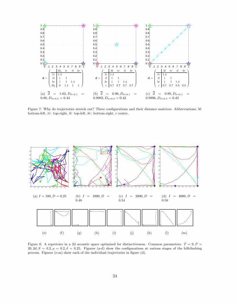
4.4 Why trajectories stretch out
Finally, in figure 7 we explore the question of why many trajectories in our simulations stretch
out. In figure (a) we show 5 signals (in the bottom-left corner there are 2 signals on top of each
other). The signals are points in the acoustic space, which we will here interpret as stationary
trajectories of some arbitrary length. The graph shows the configuration that maximises the
summed distance between the signals. The figure also gives the distance matrix, that gives for
every pair of signals the distance between them. Naturally, the values are√
2 ≈ 1.4 (across
the diagonals), 1 (horizontally or vertically) and 0 (for the pair in the bottom-left corner). The
average distance is d = 10.2/10 = 1.02.
Figure 7(b) shows an alternative configuration, with the fifth signal in the centre. The
distance matrix shows that the distance of the fifth signal to the bottom-left corner has increased,
but at the expense of the distances to the three other corners. As a result, the average distance
has actually gone down to d = 0.96. The reason is that this configuration doesn’t make optimal
use of the longest available distances over the diagonal. Importantly, however, at low noise-
levels, the distinctiveness of this configuration is in fact higher than of the configuration in (a).
The reason is that with relatively little noise and long distances, the distinctiveness–distance
function flattens out. Hence, there is more to be gained from avoiding confusion between the
fifth and the bottom-left signal, then there is from maintaining the excessive “safety margin”
with the other signals. In other words, the configuration in (b) sacrifices some average distance,
to gain a more even distribution of distances and, hence, a lower average confusion probability.
In a restricted space, increasing the distance with one sound, will usually decrease the
distance with another sound. That is, there is a crucial trade-off between maximising one
distance at the expense of another. Although maximising distinctiveness D will generally lead
to larger distances d, due to the non-linear dependence of D on d, that trade-off can work out
differently when maximising D than when maximising d.
Figure 7(c) shows yet another configuration, now with the fifth trajectory stretched out
over the whole diagonal. As is clear from the given distance matrix, this configuration yields
larger distances than in (b). To go from (b) to (c) there is no trade-off. The distances from the
central, fifth signal to the top-left and bottom-left corners can be increased without decreasing
the distances to the other two signals. The reason is that the distance between a stationary
trajectory t and a stretched out trajectory t′ is equal to the distance between t and the centroid
of t′ when t (like the top-right and bottom-left signals) is on a line through all the points of t ′,
but larger when it’s not (like the top-left and bottom-right signals). The distinctiveness in (c)
is always larger than in (b).
22

In figure 8 and 9 we show results from running the basic model under various parameter
settings, including with repertoires with many trajectories and with 3-dimensional acoustic
spaces. These results show that the observations made in the simple systems above, generalise
to a wide range of conditions.
4.5 Locally optimal repertoires are evolutionary stable strategies
So-far, we have seen that repertoires of signals with a temporal structure will, when optimised
for distinctiveness, not be organised in as many little clumps as needed, but instead stretch out.
Rather than staying away as far as possible from other trajectories along its whole length, each
trajectory will be close to some trajectories for some of its length, and close to other trajecto-
ries elsewhere. In qualitative terms, these systems show superficially combinatorial phonology.
The model represents progress from existing work, because it deals with the categorical and
combinatorial aspects as well as with the trade-off between them. It shows a possible sequence
of fit intermediates, and, hence, a route up-hill on the fitness landscape.
We have not, however, dealt with the invasibility constraint from section 2.1. Will an in-
novation be able to invade and become established in a population where it is very infrequent?
In other words: are systems that show combinatorial phonology evolutionary stable? To in-
vestigate these questions, we adapt the definition of distinctiveness to tell us something about
pairs of languages. This way we can ask the question: how well will a repertoire R ′ do when
communicating with a repertoire R? Pairwise distinctiveness D is defined as follows:
D(R,R′) =T
∑
t=1
f(d(Rt, R′t))
∑Tt′=1 f(d(Rt, R′
t′)). (14)
The quantity D(R,R′) can be interpreted as the estimated probability of a signal uttered by a
speaker with repertoire R, to be correctly interpreted by a hearer with repertoire R ′.
When we now consider the invasion of a mutant repertoire R′ into a population with resident
repertoire R, four measures are of interest: D(R,R), D(R,R′), D(R′, R) and D(R′, R′). That
is, how well does each of the repertoires fare when communicating with itself or with the
other repertoire, in the role of speaker or of hearer? Specifically, for the invasion of R ′, it is
necessary that D(R′, R) > D(R,R) or D(R,R′) > D(R,R), or some weighted combination of
these requirements (depending on the relative importance of speaking and hearing). That is,
a successful mutant must do better against the resident language, than the resident language
does against itself. Can such situations arise?
Interestingly, this situation turns out to be very common. Consider the following 1d example:
x xxx� -
repertoire A
x xx
repertoire B
The configuration on the right (B) is better on all accounts. Obviously, there will be less
23
1
1
0.9
.9
0.8
.8
0.7
.7
0.6
.6
0.5
.5
0.4
.4
0.3
.3
0.2
.2
0.1
.10
0
d =
bl1 tr tl br
tr 1.4tl 1 1br 1 1 1.4bl2 0 1.4 1 1
(a) d = 1.02, Dδ=0.1 =0.80, Dδ=0.5 = 0.44
1
1
0.9
.9
0.8
.8
0.7
.7
0.6
.6
0.5
.5
0.4
.4
0.3
.3
0.2
.2
0.1
.10
0
d =
bl tr tl br
tr 1.4tl 1 1br 1 1 1.4c 0.7 0.7 0.7 0.7
(b) d = 0.96, Dδ=0.1 =0.9993, Dδ=0.5 = 0.42
1
1
0.9
.9
0.8
.8
0.7
.7
0.6
.6
0.5
.5
0.4
.4
0.3
.3
0.2
.2
0.1
.10
0
d =
bl tr tl br
tr 1.4tl 1 1br 1 1 1.4c 0.7 0.7 0.8 0.8
(c) d = 0.99, Dδ=0.1 =0.9996, Dδ=0.5 = 0.43
Figure 7: Why do trajectories stretch out? Three configurations and their distance matrices. Abbreviations: bl:bottom-left, tr: top-right, tl: top-left, br: bottom-right, c centre.
0 0.1 0.2 0.3 0.4 0.5 0.6 0.7 0.8 0.9 10
0.1
0.2
0.3
0.4
0.5
0.6
0.7
0.8
0.9
1
(a) I = 100, D = 0.25
0 0.1 0.2 0.3 0.4 0.5 0.6 0.7 0.8 0.9 10
0.1
0.2
0.3
0.4
0.5
0.6
0.7
0.8
0.9
1
(b) I = 1000, D =0.48
0 0.1 0.2 0.3 0.4 0.5 0.6 0.7 0.8 0.9 10
0.1
0.2
0.3
0.4
0.5
0.6
0.7
0.8
0.9
1
(c) I = 2000, D =0.54
0 0.1 0.2 0.3 0.4 0.5 0.6 0.7 0.8 0.9 10
0.1
0.2
0.3
0.4
0.5
0.6
0.7
0.8
0.9
1
(d) I = 4000, D =0.58
(e) (f) (g) (h) (i) (j) (k) (l) (m)
Figure 8: A repertoire in a 2d acoustic space optimised for distinctiveness. Common parameters: T = 9, P =20, 2d, S = 0.2, ρ = 0.2, δ = 0.25. Figures (a-d) show the configurations at various stages of the hillclimbingprocess. Figures (e-m) show each of the individual trajectories in figure (d).
24

0 0.1 0.2 0.3 0.4 0.5 0.6 0.7 0.8 0.9 10
0.1
0.2
0.3
0.4
0.5
0.6
0.7
0.8
0.9
1
(a) 2d example with many tra-jectories optimised for distinc-tiveness. T = 50, P = 10, ρ =0.2, S = 0.1, δ = 0.1, I = 5000.
00.2
0.40.6
0.81
0
0.2
0.4
0.6
0.8
10
0.2
0.4
0.6
0.8
1
(b) 3d example. T = 16, P =15, ρ = 0.2, S = 0.1, δ = 0.2, I =2500, D = 0.71.
Figure 9: Repertoire in a 2d and 3d acoustic space optimised for distinctiveness.
confusion between its signals because they are further apart (when x = 0.1 and δ = 0.1,
D(A) = D(A,A) = 0.70 vs. D(B,B) = 0.84). But configuration B will even do better when
communicating with A, both as a hearer (D(A,B) = 0.78) and as a speaker (D(B,A) = 0.76).
The hillclimbing-criterion(R,R′) is redefined as follows in each of the conditions “hearer
benefits” (HB), “speaker benefits” (SB) or “equal benefits” (EB):
HB: D(R,R′) ≥ D(R,R) (15)
SB: D(R′, R) ≥ D(R,R) (16)
EB:1
2
(D (
R′, R)
+ D (
R,R′)) ≥ D(R,R) (17)
It turns out that all the stable configurations we found in simulations with the optimisation
criterion (OP, eq. 8), are also stable under criteria HB, SB and EB. Thus, locally optimal
repertoires are evolutionary stable strategies.
4.6 Not all ESSs are locally optimal
ESSs are strategies that cannot be invaded by any other strategy. In evolutionary game theory,
ESSs are therefore considered likely outcomes of an evolutionary process. However, if there
are many ESSs in a given system, the initial conditions will determine which ESS will emerge
(“equilibrium selection”). In our simulations with the HB, SB and EB conditions, we also
observe ESSs that do not correspond to the locally optimal configurations that we found with
the OP condition.
Figures 10(a-d) show the configuration of the repertoire at different numbers of iterations of
the hill-climbing algorithm under the HB condition. Figure 10(i) gives the pairwise distinctive-
25

ness measures for each combination of these 4 configurations. At the diagonal of this matrix are
the distinctiveness scores of each configuration. As is clear from this matrix, each next config-
uration can invade a population with previous repertoire. In bold-face we see the approximate
evolutionary trajectory (the actual steps in the simulation are much smaller). Figure (d) is an
ESS. However, figures (e-f) show that this configuration is not stable when the OP criterion is
used. Figure 10(j) gives the pairwise distinctiveness measures for each combination of these 5
configurations. The diagonal elements in this matrix are the highest values in their row and
column, which shows that none of these configurations could have invaded a population using
(d) under the HB (or SB, or EB) condition. Nevertheless, once adopted, communication is more
successful with every next configuration (as the diagonal elements show). The locally optimal
configuration in (f), however, is an ESS under all four conditions.
We find suboptimal ESSs in simulations with the SB and EB conditions as well. Figure 11
shows stable configurations that emerge each of the four conditions. Interestingly, these subop-
timal ESSs disappear when a different distance-to-confusion function is used. In figure 12 we
used:
f(d) =1
1 + e( 1
δd2)
, (18)
instead of equation (4). In this, and other simulations (2d and 3d) with that same function, all
ESSs observed show the same type of superficially combinatorial phonology that we found in
the OP condition.
It is difficult to evaluate the relevance of suboptimal ESSs. It appears that their existence
depends on the details of the distance-to-confusion function. Moreover, their stability depends
on the assumption of deterministic evolutionary dynamics implicit in equations (15-17). Finally,
whether or not they will emerge in evolution depends on the initial configuration.
4.7 Individual-based model
As a final test of the appropriateness of the basic model, we studied an individual-based sim-
ulation of a population of agents that each try to imitate each other in noisy conditions. This
simulation is similar to the model described above, but now each agent in the population has
its own repertoire, and it tries to optimise its own success in imitating and being imitated by
other agents of the population. Hence, a random change, as before, is applied to a random
trajectory of a random agent in the population. If this change improves the imitation success
in interaction with a number of randomly chosen other individuals in the population, it is kept.
Otherwise, it is discarded.
This version of the model is similar to the imitation games of de Boer (2000). That paper
only modelled point-like signals (vowels) and did not investigate combinatorial phonology. The
game implemented here is a slight simplification of the original imitation game. First, all agents
in the population are initialised with a random set of a fixed number of trajectories. Then
26

0 0.1 0.2 0.3 0.4 0.5 0.6 0.7 0.8 0.9 10
0.1
0.2
0.3
0.4
0.5
0.6
0.7
0.8
0.9
1
(a) t=0
0 0.1 0.2 0.3 0.4 0.5 0.6 0.7 0.8 0.9 10
0.1
0.2
0.3
0.4
0.5
0.6
0.7
0.8
0.9
1
(b) t=500
0 0.1 0.2 0.3 0.4 0.5 0.6 0.7 0.8 0.9 10
0.1
0.2
0.3
0.4
0.5
0.6
0.7
0.8
0.9
1
(c) t=1000
0 0.1 0.2 0.3 0.4 0.5 0.6 0.7 0.8 0.9 10
0.1
0.2
0.3
0.4
0.5
0.6
0.7
0.8
0.9
1
(d) t=7000
0 0.1 0.2 0.3 0.4 0.5 0.6 0.7 0.8 0.9 10
0.1
0.2
0.3
0.4
0.5
0.6
0.7
0.8
0.9
1
(e) t=10
0 0.1 0.2 0.3 0.4 0.5 0.6 0.7 0.8 0.9 10
0.1
0.2
0.3
0.4
0.5
0.6
0.7
0.8
0.9
1
(f) t=510
0 0.1 0.2 0.3 0.4 0.5 0.6 0.7 0.8 0.9 10
0.1
0.2
0.3
0.4
0.5
0.6
0.7
0.8
0.9
1
(g) t=1510
0 0.1 0.2 0.3 0.4 0.5 0.6 0.7 0.8 0.9 10
0.1
0.2
0.3
0.4
0.5
0.6
0.7
0.8
0.9
1
(h) t=6510
D∗ =
a b c d
a 0.250 0.255 0.256 0.257b 0.257 0.411 0.412 0.414c 0.260 0.412 0.443 0.445d 0.262 0.415 0.449 0.458
(i) The pairwise distinctiveness matrix
D∗ =
d e f g h
d 0.458 0.445 0.374 0.353 0.354e 0.445 0.465 0.391 0.368 0.370f 0.403 0.417 0.599 0.563 0.569g 0.387 0.400 0.564 0.629 0.614h 0.389 0.402 0.570 0.615 0.634
(j) The pairwise distinctiveness matrix
Figure 10: Locally optimal repertoires are ESSs, but not all ESSs are locally optimal. (a-d) show configurationsin an evolutionary simulation with the hearer benefit condition (HB, D(R, R′) > D(R, R)) at various timesteps; (d) is an ESS in the HB condition; (e-h) show results from a simulation in the optimisation condition(OP, D(R′, R′) > D(R, R)) that used (d) as its initial condition. (h) is an ESS in all conditions (OP, HB,SB, EB) considered. (i) shows a matrix that gives the pairwise distinctiveness scores for every combination ofconfigurations in (a-d); (j) the matrix that gives the pairwise distinctiveness scores for every combination ofconfigurations in (d-h). The approximate evolutionary trajectory is indicated with bold-face in these matrices.Parameters are: T=9, P=10, D=2, N=0.05, S=0.1.
27

0 0.1 0.2 0.3 0.4 0.5 0.6 0.7 0.8 0.9 10
0.1
0.2
0.3
0.4
0.5
0.6
0.7
0.8
0.9
1
(a) t=5000, OP
0 0.1 0.2 0.3 0.4 0.5 0.6 0.7 0.8 0.9 10
0.1
0.2
0.3
0.4
0.5
0.6
0.7
0.8
0.9
1
(b) t=5000, HB
0 0.1 0.2 0.3 0.4 0.5 0.6 0.7 0.8 0.9 10
0.1
0.2
0.3
0.4
0.5
0.6
0.7
0.8
0.9
1
(c) t=5000, SB
0 0.1 0.2 0.3 0.4 0.5 0.6 0.7 0.8 0.9 10
0.1
0.2
0.3
0.4
0.5
0.6
0.7
0.8
0.9
1
(d) t=5000, EB
Figure 11: Not all ESSs are locally optimal. Results from 4 simulations, each with the initial condition as infigure 10a. Different payoff functions lead to different ESSs, although for all payoff functions considered, locallyoptimal configurations as in (a) are stable. Parameters are: T = 9, P = 10, D = 2, ρ = 0.2, δ = 0.2, S = 0.1.
00.2
0.40.6
0.81
0
0.2
0.4
0.6
0.8
10
0.2
0.4
0.6
0.8
1
(a) t=1000
00.2
0.40.6
0.81
0
0.2
0.4
0.6
0.8
10
0.2
0.4
0.6
0.8
1
(b) t=11000
Figure 12: A 16 trajectories signal system in a 3d acoustic space, after 1000 and 11000 iterations. At each timestep, a small random change is considered, and only adopted if it represents an improvement according to thepairwise distinctiveness criterion (equation 14). Here, the confusion-probabilities are proportional to 1
1+e( 1
δd2)
,
where δ = 0.1 and d is the average segment-by-segment Euclidean distance. Parameters are: P = 15, S = 0.1, ρ =0.05, δ = 0.1. The final distinctiveness is D(R) = D(R, R) = 0.94.
28

for each game, a speaker is randomly selected from the population. This speaker selects a
trajectory, and makes a random modification to it. Then it plays a number of imitation games
(50 in all simulations reported here) with all other agents in the population. In these games,
the initiator utters the modified trajectory with additional noise. The imitator finds the closest
trajectory in its repertoire and utters it with noise. Games are successful if the imitator’s signal
is closest to the modified trajectory in the initiator’s repertoire. If it turns out that the modified
trajectory has better imitation success than the original trajectory, the modified trajectory is
kept, otherwise the original one is restored.
For vowel systems, it has been shown that optimising a single repertoire leads to similar
systems as a population-optimisation system (compare de Boer, 2000; Liljencrants and Lind-
blom, 1972). It can be shown that for trajectories the same is true, under the condition that
noisy distortions of trajectories do not distort the shape of these trajectories too much. This is
illustrated in figure 13.
0 0.2 0.4 0.6 0.8 10
0.2
0.4
0.6
0.8
1
(a)
0 0.2 0.4 0.6 0.8 10
0.2
0.4
0.6
0.8
1
(b)
0 0.1 0.2 0.3 0.4 0.5 0.6 0.7 0.8 0.9 10
0.1
0.2
0.3
0.4
0.5
0.6
0.7
0.8
0.9
1
(c)
Figure 13: Comparison of population-based models with the optimisation model. Frame (a) shows the (five)trajectories of four agents (from a population of ten), when noise preserves the shape of trajectories. Noticethe similarities with the optimised trajectories in frame (c). If noise does not preserve shape of trajectories, thetrajectories tend not to stretch out, as shown in the frame (b). Although it is rather hard to see, there are fourclusters in the corners, and one in the middle.
In this figure the left frame shows the system of five trajectories that resulted from playing
imitation games in a population, using shape-preserving noise. Frame (c), for reference, shows
a system of five trajectories that resulted from optimising distinctiveness as in the basic model.
It can be observed that in both cases, the corners are populated by four trajectories, which are
bunched up. The fifth trajectory, in contrast, follows the diagonal. As before, an analysis in
terms of phonemes suggests itself: the four corners are basic phonemes, while the fifth trajectory
uses one as the corners as a starting phoneme and the opposite corner as the ending phoneme.
Both models result in similar systems of trajectories.
The middle frame, on the other hand, shows that when noise does not preserve shape of
29

trajectories, a system results in which all trajectories are bunched up and an analysis in terms of
phonemes is therefore not possible. As noise in real signals is band limited, it follows that shape
will always be preserved to some extent. For computational reasons, we have not performed
simulations in the population condition with more than 5 trajectories. However, although less
clean and not fully conclusive, the results from the individual-based model seem to be consistent
with the observations with the basic model.
4.8 Measuring combinatorial phonology
So far, we have relied on an intuitive notion of what it means for a repertoire of trajectories
to show combinatorial phonology. As the paper investigates the emergence of categorical and
combinatorial coding on a qualitative level, this has not been an obstacle. However, for a more
quantitative understanding of the emergence of combinatorial phonology, a numerical measure
of the degree of recombination would be useful. When the basic building blocks of the repertoire
are known, it is straightforward to give a measure of the degree of combination. An example
would be the number of times a given building block is being reused: ϕ = Nk
, where ϕ is the
measure of recombination (phonemicity), N is the number of words in the repertoire and k the
number of building blocks.
A difficult problem, however, is finding the basic building blocks, given a repertoire of signals.
The traditional linguistic procedure for indentifying phonemes in an unknown language, relies
on the notion of “minimal pair”: a pair of words that have different meanings and differ only
in one sound. An example would be the English pair “keel” and “cool”. Hence, an hypothesis
on a candidate phoneme can be validated by providing a minimal pair that differs only in that
phoneme.
This analysis might seem straightforward, but when put to use in an automatic phoneme
discovery procedure, a number of pitfalls emerge. First of all, it already makes use of an existing
set of basic building blocks (usually the phonetic categories as defined by the International
Phonetic Association). Secondly, it needs to decide what is meaningful variation and what is
variation caused by automatic influence from neighbouring sounds. In the example, the k-like
sounds at the beginning of the words are different, too, but it is generally accepted that this is
due to the influence of the vowels that follow. They are said to be allophones. However, this
can only be deduced from the physics of articulation, not from the signals themselves.
A final problem in the analysis is how to decide that two building blocks are equal. In the
case of the two different k-sounds, it can be argued that they are instances of the same building
block, because there are no minimal pairs and their articulation is very similar. However, the
case is not so clear-cut for other examples. A well-known example is the case of English “h”
and “ng”. The former occurs only at the beginning of syllables, and the latter occurs only at
the end. There are therefore no minimal pairs, and they could be considered allophones, but
30

because of their articulatory differences, this is never done. There are cases in other languages
that are even more problematic, and it is not uncommon to find disagreement amongst linguists
about the exact set of building blocks that are used in a language.
In the case of artificially generated sets of trajectories, these problems are even more ap-
parent. One needs to make assumptions about what kind of building blocks are possible, what
constitutes natural behaviour for a trajectory between building blocks, and how to define sim-
ilarity between building blocks. In the analyses that we have presented, we have implicitly
assumed that building blocks are points, that trajectories tend to follow straight lines from
point to point and that points that are close together are the same building block. We do
not yet know how to automate the process of extracting building blocks and therefore cannot
calculate the phonemicity of a repertoire automatically.
5 Discussion and Conclusion
We have shown that optimising trajectories for acoustic distinctiveness results in superficial
combinatorial phonology. When optimising a repertoire of temporally extended trajectories in
an abstract acoustic space, the trajectories tend either to occupy the corners of the available
space or to stretch out from corner to corner. It appears as if trajectories become far apart where
possible and close together where necessary. A repertoire with this structure can be analysed
as reusing certain points as building blocks of its trajectories and thus to have combinatorial
structure. As there is nothing in the trajectory that explicitly codes this structure and as
agents that would use these repertoires of trajectories need not be aware of their structure,
their combinatorial nature is purely superficial.
Most of the results presented here were obtained through direct optimisation of repertoires
of trajectories. However, we have also shown that superficially combinatorial repertoires of
trajectories can emerge in a population of agents that try to imitate each other as well as
possible. Apparently agents that strive for maximum success in imitation in noisy conditions,
using information from simple interactions (imitation games) alone, converge towards repertoires
that are similar to repertoires that are optimised directly.
Finally, we have shown that repertoires of trajectories that are optimised for acoustic dis-
tinctiveness (and thus combinatorial) are evolutionary stable. Agents that have a repertoire of
trajectories that is more optimised for acoustic distinctiveness can invade a population of agents
that have less optimal (but otherwise similar) repertoires, at least if the only fitness criterion
is the robustness to acoustic noise of their repertoires. Conversely, a population of agents with
an optimal repertoire cannot be invaded by agents with less optimal repertoires. We have also
shown that there is a path of ever increasing fitness towards the optimal (and combinatorial)
repertoire.
Our model differs from other attempts to explain combinatorial speech in several ways.
31

First of all, both holistic and (superficially) combinatorial signals have temporal structure. All
signals in the model are of the same duration. Secondly, our model does not use articulatory
targets. The resulting structure is purely emergent and therefore called “superficial”. In fact,
no distinction is made between holistic and combinatorial signals in the model; the difference
only becomes apparent when analysing the structure of the repertoires.
We argue that agents can make use of this structure to evolve towards productive use of
recombination. When the structure becomes available in the population, it becomes advanta-
geous for agents to make use of it. They can use it to store the repertoire of trajectories more
compactly, to perceive and produce trajectories in a more robust way and eventually to more
easily create new trajectories. In this way, agents that use combinatorial structure productively
can invade a population of agents that do not. This is only possible when there already exists
a repertoire that is superficially combinatorial. Only then is there a path of continuously in-
creasing fitness towards productive combinatorial coding, and eventually, to phonemic speech.
We have shown that optimisation for acoustic distinctiveness can result in such a repertoire.
Natural language phonology is categorical and combinatorial. What we have shown in this
paper is that these properties have functional significance: they aid the reliable recognition of
signals by the hearer. We have also shown that there is a path that leads from a signal system
without these properties, to one with those properties. Crucially, we have shown that each step
on this path represents an improvement, both when it first appears in a population and when
it is already common.
It turns out that a categorical and combinatorial system of speech sounds is advantageous
even for a population of speakers and listeners that is not aware of this structure. Thus com-
binatorial structure can emerge in a culturally transmitted system of calls before there are
cognitive (genetic) adaptations for using this structure. This makes it unnecessary for combi-
natorial phonology to have emerged through purely genetic evolution. Rather, natural selection
shapes the parameters of the self-organising process and cultural self-organisation determines
what genetic adaptations will be beneficial. Hence, self-organisation is the substrate of evolution
(Waddington, 1939; Boerlijst and Hogeweg, 1991; Kirby and Hurford, 1997; Smith, 2004).
Acknowledgements WZ is funded by the Netherlands Organisation for Scientific Research
(Exacte Wetenschappen), project number 612.066.405. Part of this research was performed
whilst WZ was at the Language Evolution and Computation research unit and the Institute of
Evolutionary Biology of the University of Edinburgh. We like to thank Nick Barton, Jim Hur-
ford, Simon Kirby, Matina Donaldson, Tecumseh Fitch and Mark Steedman for their comments
on earlier drafts of this paper.
32

References
Arcadi, A. (1996). Phrase structure of wild chimpanzeepant hoots: patterns of production and interpopula-tion variability. Am. J. Primatol, 39:159–178.
Boerlijst, M. and Hogeweg, P. (1991). Self-structuringand selection: Spiral waves as a substrate for prebi-otic evolution. In Langton, C., Tayler, C., Farmer, J.,and Rasmussen, S., (Eds.), Artificial Life II, pages255–276.
Bogert, B. P., Healy, M. J., and Tukey, J. W. (1963).The quefrency analysis of time series for echoes: cep-strum, pseudo-autocovariance, cross-cepstrum, andshape cracking. In Rosenblatt, M., (Ed.), Time Se-ries Analysis, pages 209–243. J. Wiley, New York,NY.
Carlson, R., Granstrom, B., and Fant, G. (1970). Somestudies concerning perception of isolated vowels. InSpeech Transmission Laboratory Quarterly Progressand Status Report, volume 2-3, pages 19–35. RoyalInstitute of Technology, Stockholm, Sweden.
Chomsky, N. and Halle, M. (1968). The sound patternof English. Harper & Row, New York, NY.
Cooper, F. S., Delattre, P. C., Liberman, A. M., Borst,J. M., and Gerstman, L. J. (1952). Some experimentson the perception of synthetic speech sounds. Jour-nal of the Acoustical Society of America, 24:597–606.
de Boer, B. (1999). Self Organisation in Vowel Sys-tems. PhD thesis, Artificial Intelligence Lab, VrijeUniversiteit Brussel.
de Boer, B. (2000). Self organization in vowel systems.Journal of Phonetics, 28:441–465.
de Boer, B. (2001). The origins of vowel systems. Ox-ford University Press, Oxford, UK.
Deuchar, M. (1996). Spoken language and sign lan-guage. In Lock, A. and Peters, C. R., (Eds.), Hand-book of Human Symbolic Evolution. Clarendon Press,Oxford, UK.
Doupe, A. J. and Kuhl, P. K. (1999). Birdsong andhuman speech: Common themes and mechanisms.Annual Review of Neuroscience, 22:567–631.
Fitch, W. T. (2000). The evolution of speech: a compar-ative review. Trends in Cognitive Science, 4(7):258–267.
Harnad, S., (Ed.) (1987). Categorical Perception:the groundwork of cognition. Cambridge UniversityPress, Cambridge, UK.
Hauser, M. D. (1996). The Evolution of Communica-tion. Bradford/MIT Press, Cambridge, MA.
Hockett, C. (1960). The origin of speech. ScientificAmerican, 203:88–111.
Jackendoff, R. (2002). Foundations of Language. Ox-ford University Press, Oxford, UK.
Jager, G. (2005). Evolutionary game theory for lin-guists. a primer. Technical report, Stanford Univer-sity and University of Potsdam.
Ke, J., Ogura, M., and Wang, W. S.-Y. (2003). Mod-eling evolution of sound systems with genetic algo-rithm. Computational Linguistics, 29(1):1–18.
Kirby, S. and Hurford, J. (1997). Learning, culture andevolution in the origin of linguistic constraints. In
Husbands, P. and Harvey, I., (Eds.), Proceedings 4thEuropean Conference on Artificial Life, pages 493–502. MIT Press, Cambridge, MA.
Komarova, N. L. and Nowak, M. A. (2003). Language,learning and evolution. In Christiansen, M. H. andKirby, S., (Eds.), Language Evolution, pages 317–337. Oxford University Press, Oxford, UK.
Kuhl, P., Williams, K., Lacerda, F., Stevens, K., andLindblom, B. (1992). Linguistic experience altersphonetic perception in infants by 6 month of age.Science, 255:606–608.
Levelt, W. and Wheeldon, L. (1994). Do speakershave access to a mental syllabary? Cognition, 50(1-3):239–69.
Lieberman, P. (1984). The biology and evolution of lan-guage. Harvard University Press, Cambridge, MA.
Liljencrants, J. and Lindblom, B. (1972). Numericalsimulations of vowel quality systems: the role of per-ceptual contrast. Language, 48:839–862.
Lindblom, B., MacNeilage, P., and Studdert-Kennedy,M. (1984). Self-organizing processes and the expla-nation of phonological universals. In Butterworth,B., Comrie, B., and Dahl, O., (Eds.), Explanationsfor Language Universals, pages 181–203. Mouton,Berlin.
MacNeilage, P. F. and Davis, B. L. (2000). On theorigin of internal structure of word forms. Science,288:527–531.
Masataka, N. (1987). The perception of sex-specificityin the long calls of the tamarin (saguinnes labiatuslabiatus). Ethology, 76:56–64.
Maynard Smith, J. (1982). Evolution and the Theoryof Games. Cambridge University Press, Cambridge,England.
Maynard Smith, J. and Price, G. R. (1973). The logicof animal conflict. Nature, 246:15–18.
Mitani, J. C. and Marler, P. (1989). A phonologicalanalysis of male gibbon singing behavior. Behaviour,109:20–45.
Nowak, M. A., Krakauer, D., and Dress, A. (1999). Anerror limit for the evolution of language. Proceedingsof The Royal Society of London. Series B, BiologicalSciences, 266(1433):2131–2136.
Nowak, M. A. and Krakauer, D. C. (1999). The evo-lution of language. Proc. Nat. Acad. Sci. USA,96:8028–8033.
Oudeyer, P.-Y. (2001). Coupled neural maps for theorigins of vowel systems. In G. Dorffner, H. Bischof,K. H., (Ed.), Proceedings of the International Con-ference on Artificial Neural Networks, LNCS 2130,pages 1171–1176. Springer Verlag, Berlin.
Oudeyer, P.-Y. (2002). Phonemic coding might be aresult of sensory-motor coupling dynamics. In Hal-lam, B., Floreano, D., Hallam, J., Hayes, G., andMeyer, J.-A., (Eds.), Proceedings of the 7th Interna-tional Conference on the Simulation of Adaptive Be-havior, pages 406–416. MIT Press, Cambridge, MA.
Oudeyer, P.-Y. (2005). The self-organization of speechsounds. Journal of Theoretical Biology, 233(3):435–449.
33

Parker, G. A. and Maynard Smith, J. (1990). Optimal-ity theory in evolutionary biology. Nature, 348:27–33.
Payne, R. S. and McVay, S. (1971). Songs of humpbackwhales. Science, 173(3997):585–597.
Pierrehumbert, J. (2001). Exemplar dynamics: Wordfrequency, lenition, and contrast. In Bybee, J. andHopper, P., (Eds.), Frequency effects and the emer-gence of linguistic structure, pages 137–57. John Ben-jamins, Amsterdam, the Netherlands.
Plotkin, J. B. and Nowak, M. A. (2000). Language evo-lution and information theory. Journal of TheoreticalBiology, pages 147–159.
Redford, M. A., Chen, C. C., and Miikkulainen, R.(2001). Constrained emergence of universals andvariation in syllable systems. Language and Speech,44:27–56.
Sakoe, H. and Chiba, S. (1978). Dynamic programmingoptimization for spoken word recognition. IEEETransactions on Acoustics, Speech and Signal Pro-cessing, 26(1):43–49.
Shannon, C. E. (1948). A mathematical theory of com-munication. The Bell Systems Technical Journal,27(July, October):379–423 and 623–656.
Smith, K. (2004). The evolution of vocabulary. Journalof Theoretical Biology, 228(1):127–142.
Steels, L. and Oudeyer, P.-Y. (2000). The cultural evo-lution of syntactic constraints in phonology. In Be-dau, M. A., McCaskill, J. S., Packard, N. H., andRasmussen, S., (Eds.), Proceedings of the VIIth Arti-ficial life conference (Alife 7). MIT Press, Cambridge(MA).
Studdert-Kennedy, M. (1998). The particulate ori-gins of language generativity: from syllable to ges-
ture. In Hurford, J. R., Studdert-Kennedy, M., andKnight, C., (Eds.), Approaches to the evolution oflanguage: social and cognitive bases. Cambridge Uni-versity Press, Cambridge, UK.
Studdert-Kennedy, M. (2002). Mirror neurons, vocalimitation and the evolution of particulate speech. InStamenov, M. and Gallese, V., (Eds.), Mirror Neu-rons and the Evolution of the Brain and Language,pages 207–227. John Benjamins, Amsterdam.
Tinbergen, N. (1963). On aims and methods of ethol-ogy. Zeitschrift fur Tierpsychologie, 20:410–433.
Ujhelyi, M. (1996). Is there any intermediate stage be-tween animal communication and language? Journalof Theoretical Biology, 180:71–76.
van Rooij, R. (2004). Evolution of conventional mean-ing and conversational principles. Synthese (Knowl-edge, Rationality and Action), 139:331–366.
Waddington, C. H. (1939). An Introduction to ModernGenetics. Allen Unwin, London.
Westermann, G. (2001). A model of perceptual changeby domain integration. In Proceedings of the 23dAnnual Conference of the Cognitive Science Society.Lawrence Erlbaum, Mahwah, NJ.
Westermann, G. and Miranda, E. (2004). A newmodel of sensorimotor coupling in the developmentof speech. Brain and Language, 89:393–400.
Zuidema, W. (2005). The major transitions in the evo-lution of language. PhD thesis, Theoretical and Ap-plied Linguistics, University of Edinburgh.
Zuidema, W. and de Boer, B. (2003). How did we getfrom there to here in the evolution of language? Be-havioral and Brain Sciences, 26(6):694–695.
34