the european refinery industry under the eu emissions trading scheme

J U L I A R E I N A U D

November 2005

THE EUROPEAN REFINERY INDUSTRY UNDERTHE EU EMISSIONS TRADING SCHEME

Competitiveness, trade flowsand investment implications

INTERNATIONAL ENERGY AGENCYAGENCE INTERNATIONALE DE L’ENERGIE

IEA INFORMATION PAPER

3

ACKNOWLEDGEMENTS

Julia Reinaud is the principal author of this paper. The author would like to thank Pierre Becard (Astra) and Richard Baron for very useful suggestions and advice. The author would also like to thank Toril Bosoni, Richard Bradley, Sylvie Cornot, Cintia Gavay, Lawrence Eagles, David Fyfe, Noé van Hulst, Isabel Murray, Marek Struck (IEA), Jean François Larivé (Concawe), Jean Francois Gruson (IFP), Jean-Gaël Le Floc’h, Serge Mennecier, Francis Nativel, (Axens), Régis Collieux (BNPParibas), and BIAC for the information, comments and ideas they provided throughout this research.

The ideas expressed in this paper are those of the author and do not necessarily represent views of the IEA or its member countries.

5

TABLE OF CONTENTS

ACKNOWLEDGEMENTS ............................................................................................................................................3

TABLE OF CONTENTS...............................................................................................................................................5

EXECUTIVE SUMMARY.............................................................................................................................................9

INTRODUCTION.......................................................................................................................................................13

1. The EU Emissions Trading Scheme ......................................................................................................... 15 1.1 History and context........................................................................................................................................ 15 1.2 Main design features...................................................................................................................................... 16 2. Profile of the European Refinery Industry.............................................................................................. 19 2.1 General profile of the refinery industry ...................................................................................................... 19 2.2 The European refinery industry: upstream input...................................................................................... 19 2.3 European refinery units ................................................................................................................................ 22 2.4 Downstream products in Europe ................................................................................................................. 23 2.5 Environmental specifications in Europe...................................................................................................... 26 2.6 International product flows .......................................................................................................................... 27 3. Methodology ............................................................................................................................................... 29 3.1 Selecting representative European refinery units ...................................................................................... 29 3.2 Evaluating the impacts of a grandfathered C02 allocation ........................................................................ 30 4. CO2 Emissions in European Refineries: Case Studies Assumptions..................................................... 33 4.1 Upstream input .............................................................................................................................................. 33 4.2 Downstream products.................................................................................................................................... 34 4.3 Energy consumption ...................................................................................................................................... 35 4.3.1 Electricity and steam .................................................................................................................................. 35 4.3.2 Hydrogen production and consumption................................................................................................... 36 4.4 Energy related CO2 Emissions...................................................................................................................... 37 4.4.1 CO2 emissions by process units.................................................................................................................. 37 4.4.2 CO2 emissions by finished products .......................................................................................................... 39 4.5 Profitability of the sector in Europe............................................................................................................. 40 4.5.1 Costs in refineries........................................................................................................................................ 40 4.5.2 Revenues in refineries................................................................................................................................. 41 4.5.3 Net margins for refineries .......................................................................................................................... 41 5. Competitiveness Impacts of the EU ETS on the European Refinery Industry.................................... 43 5.1 Auto production of electricity....................................................................................................................... 43 5.2 Purchasing electricity scenario: impacts of higher electricity prices ....................................................... 44 5.3 Auto-generating with an Integrated Gasification Combined Cycle (IGCC) scenario ............................ 54 5.4 Prices for end-products ................................................................................................................................. 56 6. Comparison of CO2 costs with investment costs in desulphurisation .................................................. 59 6.1 Investment costs in desulphurisation technologies to meet the European specifications ....................... 59 6.1.1 Upgrading hydro-skimming refineries ..................................................................................................... 61 6.1.2 HSK + FCC configuration ......................................................................................................................... 62 6.2 Political questions .......................................................................................................................................... 63 6.3 Extra available capacity to meet increased exports - construction or expansion of refineries outside of Europe................................................................................................................................................................... 63 7. Consequences on trade flows: a re-distribution of locations or a change in production strategies? . 65 7.1 Increase of foreign imports into Europe...................................................................................................... 65 7.2 Change in production strategy ..................................................................................................................... 65 7.3 Change in crude oil feedstock....................................................................................................................... 66 8. Euro 5 standards for European refinery products: impacts on investments and emissions ............. 69 CONCLUSION ..........................................................................................................................................................73 GLOSSARY ............................................................................................................................................................. 77

6

TABLES Table 1: Different Refinery Configurations .......................................................................................................... 20 Table 2: Refinery breakdown in Europe by technology (2004) ............................................................................ 23 Table 3: Trade of refined products in 2004 for EU 19 .......................................................................................... 28 Table 4: Share of main crude oil imports per European region in 2004 ............................................................... 33 Table 5: Gross refinery output per region (2003) .................................................................................................. 34 Table 6: Energy requirements by configuration .................................................................................................... 37 Table 7: Emission factors of refinery fuels............................................................................................................ 38 Table 8: CO2 Emissions per configuration in NWE as wt% of total emissions.................................................... 38 Table 9: CO2 emissions per finished product......................................................................................................... 39 Table 10: Total CO2 emissions per region and configuration ............................................................................... 40 Table 11: Refinery margin calculations (valued at regional prices)...................................................................... 41 Table 12: Opportunity cost of CO2 emissions per barrel of crude oil input.......................................................... 44 Table 13: CO2 emissions and refinery margins assuming full purchase of electricity.......................................... 46 Table 14: Increase in electricity prices under full pass-through of CO2 prices on wholesale prices .................... 49 Table 15: Decrease in refinery margins following inclusion of direct and indirect cost of CO2 .......................... 49 Table 16: Summary of scenario results on power supply, assuming full opportunity cost of CO2 ...................... 53 Table 17: Summary of scenario results on power supply, assuming 2 or 10% of CO2 purchase ......................... 54 Table 18: Residue gasification and electricity/hydrogen production .................................................................... 55 Table 19: Changes in refinery output, margins and CO2 emissions following investment in an IGCC................... 56 Table 20: Changes in refinery margins of a complex refinery with IGCC when direct and indirect impact of CO2

emissions are accounted for........................................................................................................................... 57 Table 21: Share of imports from European countries (2003)................................................................................ 58 Table 22: Russian construction update .................................................................................................................. 60 Table 23: Major differences in produced fuels characteristics between Russia and Europe ............................... 60 Table 24: Required capacities and investments for Euro 5 specification – Russian HSK .................................... 61 Table 25: Required capacities and investments for Euro 5 specification production – Russian HSK + FCC...... 62 Table 26: HSK + VB + FCC refinery mass balance, M-100 processing .............................................................. 66 Table 27: HSK + VB + FCC refinery margins, M-100 processing....................................................................... 67 Table 28: Required capacity investments to reach Euro V specifications – North West Europe HSK+FCC+VB

configuration.................................................................................................................................................. 70 Table 29: HSK+VB+FCC hydrogen mass balance ............................................................................................... 71 Table 30: Examples of process units in a refinery................................................................................................. 85 Table 31: 2004 Refinery breakdown in Europe by technology............................................................................. 88 Table 32: Crude oil and refinery feedstock prices ................................................................................................. 95 Table 33: Prices based on Platts year 2004 ........................................................................................................... 96 Table 34: Euro 2, 3 and 4 specifications................................................................................................................ 97 Table 35: Quality of gasoline and diesel in Europe............................................................................................... 98 Table 36: Quality of heating oil and fuel oil in Europe ......................................................................................... 99 Table 37: Product specifications.......................................................................................................................... 100 Table 38: Russian HSK capacities taken into account, and required capacities to meet Euro V specifications 111 Table 39: Russian HSK+ FCC capacities taken into account, and required capacities to meet Euro V

specifications ............................................................................................................................................... 112

7

FIGURES Figure 1: Crude oil imports in OECD Europe ....................................................................................................... 21 Figure 2: Crude oil quality by types ...................................................................................................................... 22 Figure 3: Typical product yield in 2002 ................................................................................................................ 24 Figure 4: Demand for refined products in OECD Europe (1971-2004)................................................................ 24 Figure 5: gasoil/fuel oil spread in north western europe ....................................................................................... 25 Figure 6: Clean product demand forecast .............................................................................................................. 25 Figure 7: Comparison of required specifications for gasoline and diesel ............................................................. 26 Figure 8: CO2 Emission increases following higher environmental specifications............................................... 27 Figure 9: Accounting for CO2 cost ........................................................................................................................ 31 Figure 10: Fuel mix for refineries across OECD Europe and EU-15.................................................................... 35 Figure 11: Refinery gas and refinery fuel oil share in refineries across OECD countries .................................... 36 Figure 12: Average natural gas import prices in Europe ....................................................................................... 37 Figure 13: Impacts of full CO2 cost accounting on refinery margins.................................................................... 45 Figure 14: Impacts on refinery margins: from full cost to real cost accounting of CO2 ....................................... 45 Figure 15: Refinery margins under various electricity supply assumptions ......................................................... 50 Figure 16: Global upgrading unit capacity ............................................................................................................ 63 Figure 17: Global upgrading capacity: historical evolution and forecast.............................................................. 64 Figure 18: The oil refinery process and output...................................................................................................... 85 Figure 19: Crude oil imports in OECD Europe from OPEC ............................................................................... 103 Figure 20: Crude oil imports in OECD Europe from Former Soviet Union ....................................................... 103 Figure 21: Imports from Russia into OECD Europe from 1995 to 2004 ............................................................ 117 Figure 22: Evolution of freight rates for dirty vessels between Europe, Black Sea and Baltic Sea from 2002 to

2004.............................................................................................................................................................. 119 Figure 23: Evolution of clean vessels’ freight rates between the Black Sea, Baltic Sea and Europe ................. 120

ANNEXES ANNEX 1: REFINERY PRODUCTS ............................................................................................................................. 79 ANNEX 2: REFINERY CONFIGURATIONS ................................................................................................................. 80 ANNEX 3: AN INTRODUCTION TO THE REFINERY SECTOR ....................................................................................... 84 ANNEX 4: NUMBER OF REFINERY CONFIGURATIONS BY EU-25 COUNTRY............................................................ 88 ANNEX 5: REFINERY CAPACITY UTILISATION RATE IN OECD COUNTRIES........................................................... 89 ANNEX 6: CRUDE INPUT FOR EACH REFINERY CONFIGURATION, ACCORDING TO REGION ...................................... 90 ANNEX 7: CALCULATED REFINERY PRODUCTION................................................................................................... 91 ANNEX 8: REFINERY PROCESS FUELS COMPOSITION BY REGION AND CONFIGURATION.......................................... 93 ANNEX 9: CRUDE OIL AND REFINERY FEEDSTOCK PRICES ...................................................................................... 95 ANNEX 10: PRODUCT SPECIFICATIONS ................................................................................................................... 97 ANNEX 11: RUNNING EXPENSES AND INVESTMENT COSTS PER AREA AND CONFIGURATION ............................... 102 ANNEX 12: CRUDE OIL IN EUROPE....................................................................................................................... 103 ANNEX 13: MAIN COUNTRIES IMPORTING AND EXPORTING REFINED OIL PRODUCTS INTO AND FROM OECD

EUROPE......................................................................................................................................................... 105 ANNEX 14: REFINERY PROJECTS AND ASSOCIATED COSTS.................................................................................. 109 ANNEX 15: QUALITY OF THE HFO M-100 ASSUMMED IN THE CASE STUDY ......................................................... 110 ANNEX 16: INVESTMENT IN RUSSIAN REFINERIES TO MEET EURO V SPECIFICATIONS........................................ 111 ANNEX 17: REFINERY FUEL COMPOSITION .......................................................................................................... 113 ANNEX 18: AACE COST ESTIMATE CLASSIFICATION .......................................................................................... 116 ANNEX 19: FORMER SOVIET UNION AND RUSSIA ................................................................................................ 117 ANNEX 20: ASSUMPTIONS ON THE ALLOCATION OF CO2 EMISSIONS TO REFINERY PRODUCTS ............................. 118 ANNEX 21: THE FREIGHT PRICE DIFFERENTIAL FROM A STATIC POINT OF VIEW ................................................... 119

9

EXECUTIVE SUMMARY

Objective

The Kyoto Protocol establishes emission constraints for a number of IEA member countries, and all EU member states. The EU emissions trading scheme (EU ETS) is the primary instrument to control industrial CO2 emissions from energy through an allocation of allowances to some 11 500 installations. As such, the EU ETS applies only to a subset of countries whose industry, in some cases, competes with producers without greenhouse gas constraints, a source of concern for industry and policy makers alike. This study seeks to analyse this issue in the specific case of the EU oil refinery sector.1

We assess short to medium term impacts of a carbon cost introduced by emissions trading, from the standpoint of international cost competitiveness and profitability, looking at a range of representative refinery configurations in three European regions. An important element is the industry’s ability to pass carbon cost increases to their product prices.

This work does not evaluate emissions trading relative to other measures; this would require comparing this instrument with policy alternatives that could deliver a similar environmental outcome (a tax, or a set of command-and-control measures). This is beyond the scope of this work.

Methodology

The study is based on case studies that distinguish plant configurations, crude oil inputs, and production patterns, all specified within each of the three regions: northwest, central and Mediterranean. The diversity of refinery units, their crude oil inputs, and production yields prohibit the use of a single configuration for Europe’s refinery industry. For the sake of realism, input and output volumes, as well as refining capacities, are based on 2003-2004 data. However, assumptions were made on product yields for each configuration, as no public data exist.

The price of CO2 emissions is part of a plant’s variable costs. The production of an intermediate or finished product generates CO2 for which the foregone opportunity is the option to sell allowances – whether distributed for free or purchased from the market. The marginal cost of carbon allowances should therefore be treated as variable cost and fully passed on to production costs. In practice, however, grandfathered allowances (distributed for free in the allocation process) do not impose cash costs. In a short term perspective, the only cash costs stem from the purchase of allowances to match potential emissions above the initial allocation, and the costs of implementing emission reductions internally.

Nevertheless, we evaluate the effects of a CO2 cap with three scenarios. The first assumes the full pass through of allowance prices in production costs (as if allowances were treated as a carbon tax). We then consider the cost of 2% and 10% shortfalls of allowances, which plants would be required to purchase from the carbon market.

No view is given on the scope for internal emission reductions. Since it is not possible to predict to which degree plants or companies will undertake abatement investments to meet their objective and to which degree they will rely on the market to comply, we assume that every avoided emission carries a cost equal to the allowance market price. This leads to overestimating near-term compliance costs:

1. in theory, sources invest in internal reductions that are less expensive than the market price;

1 See Reinaud, 2003, 2004 for analyses of other sectors.

10

2. some sources, in so doing, become net sellers and therefore offset part of their investment. Our aim is therefore only to provide upper bounds for orders of magnitude, i.e.,, not to predict compliance costs under the EU ETS.

We also consider the economics of auto-production of electricity versus electricity purchases from the grid. However, the decision to auto-produce electricity is only available at the project design phase: the choice is largely irreversible from thereon.

The European refining industry is assumed to be price-taker on crude oil and some refinery product markets. For those products, any cost incurred to respond to the CO2 constraint should reduce profit margins or trigger cost reductions elsewhere. Refiners may nevertheless restore their profit margins by further lowering other operational costs (e.g.,, labour costs; energy consumption; and maintenance cost) and by optimising the crude slate (the mix of crude oil with different physical specifications) and finished products pattern.

Main results

The opportunity cost of CO2 allowances is not trivial for the refining industry under the full pass through scenario - at EUR 10/tCO2, the CO2 cost would amount to 15 to 30% of total running expenses. At EUR 20/tCO2, the cost of carbon would reach about USD 1 per barrel of crude oil entering the refinery, a substantial part of projected refining margins.2 In comparison, refinery margins in this study range between USD -1 and USD +6/bbl assuming a price of Brent crude at USD 43/bbl.

The picture differs substantially once grandfathered allowances are taken into account on the cost side. In our 10% shortfall scenario, CO2 costs would amount to 1-3% of running costs.

Companies’ perception of the cost of CO2 in a long-term perspective is therefore crucial to understand how emissions trading will eventually affect refiners’ investment decisions. Treating EU ETS allocations on a cash cost basis, rather than a full opportunity cost basis, only reflects a short-term perspective. On the other hand, the EU ETS does not envision a full auctioning of allowances before long (only a maximum of 10% may be sold to installations in 2008-2012). For as long as new entrants have access to free reserves of allowances, their incentive to relocate ought to be limited.

On the other hand, the impact of the EU ETS may be exacerbated for refineries that purchase electricity from the grid, as electricity prices are growing with the CO2 constraint that now applies to power generators. The current market structure in Europe and the practice of marginal cost pricing in power generation should lead to the pass through of the carbon opportunity cost to wholesale markets. There are good theoretical reasons to believe that CO2 prices should not be fully passed-through under the EU emissions trading scheme, such as a repetitive allocation process that somewhat discourages mitigation, the degree of competition in the power market, and the treatment of new entrants. Differences in existing electricity prices across Europe trigger different effects from the CO2 constraint on refining economics.

In our analysis, for refineries in northwest and central Europe, purchases from the grid entail higher refinery margins than in the Mediterranean region. Power prices are lower than the cost of internal electricity production in those regions, even if we assume a full pass through of the opportunity cost of CO2 allowances to wholesale prices. In contrast, refinery margins in the

2 At the time this report was completed, EU allowances were traded at EUR 22/tCO2.

11

Mediterranean area are lower if power is purchased from the grid in simple refinery configurations. This is also true for the most complex configuration, until the price of CO2 allowances reaches EUR 50/tCO2. It would then be more economic to purchase power from the grid. The power supply strategy is not as straightforward if refineries only account for the cash cost of purchasing allowances above their grandfathered quotas (i.e.,, 2 or 10% scenarios). The choice of power supply (auto-production or grid) would hinge on conditions for new entrants in the trading scheme.

Auto-production of electricity from an integrated gasification combined cycle (IGCC) plant is only economic in the Mediterranean area where electricity prices are higher (EUR 40/MWh on average in 2004). IGCC implementation only slightly decreases the refinery margin by 1%.

Since mid-2004, the European refining industry is in a positive cycle. In such circumstances, any increase in cost as the result of the CO2 constraint may be alleviated by a strong demand for refinery products in high growth regions with insufficient refining capacity (China, Asia, and North America), as product prices grow rapidly. Amortising any CO2 cost should be evaluated in this pricing environment. In the near term, the moderate cash cost imposed by the CO2 cap is unlikely to represent an obstacle to European gasoline exports to foreign markets, especially North America, where demand is strong.

Another factor affects product prices and their evolution under a carbon constraint. Several European countries are supplied in certain products by European refineries almost exclusively; e.g., aviation gasoline, kerosene, etc. It is conceivable that European refineries aremain players in these markets and would thus have the possibility to pass on most if not all of their CO2 cost to consumers – either the actual cash costs or the full opportunity cost, as witnessed in electricity markets.

A rise in European prices may in turn increase the price of European products, encouraging foreign products imports. However, at the moment, there is no clear signal that imports of finished products will increase as a direct result of the CO2 constraint. Investment in desulphurisation (amounting to USD 2-4 per barrel) will be necessary for foreign finished products to be in compliance with European specifications and to be granted access to the EU market. Changes in product patterns and in feedstock strategy towards lower emissions may occur as a consequence of the carbon constraint. For example, European refiners could import more semi-processed products (such as Russian fuels) to lower their CO2 emissions. Freight costs would not constitute a barrier, as freight rates for these “dirty” products are cheaper than those for clean products.

European environmental specifications are pushing for more advanced and more CO2 intensive refinery processes, potentially exacerbating the impact of the CO2 price. The oil industry argues that not all Member States have assigned allowances to their refining industry with full account taken of this evolution – as was suggested by the Commission guidance paper. If so, operators in these countries would face the combined challenge of investing in more CO2-intensive units to process cleaner fuels, while facing a fixed cap on their emissions. This scenario has not been studied here.

CO2 emissions for a refinery vary with its fuel consumption. To the extent that a refinery can burn more natural gas, the increase in use of natural gas in an attempt to stay within the cap will put

12

pressure on other sectors needing the same fuel, notably power producers. This may exacerbate pressure on gas prices, electricity and other energy intensive products. However, this effect could be mitigated by a growing price differential between natural gas and HFO, at that advantage of the latter, in spite of its higher carbon content. Assessing this scenario was beyond our scope.

Caveats

No data exist on the segmentation of crude used in different refinery configurations. In principle, though, it is realistic to assume that the more complex the refinery, the heavier the crude it processes – although regional disparities are important. Our assumptions for this study were based on country-level imports data for various crude oils.

There is no straightforward, incontestable methodology to allocate CO2 emissions to final products. The results per product must therefore be interpreted with great care. In general and on average, gasoline production through catalytic cracking is much more energy-intensive and CO2-intensive than diesel through primary distillation. This may not hold true when we consider marginal incremental production of one product versus the other which imply incremental investments in processing units converting heavy fuel oil into lighter transport fuels.

Net refinery margins calculated from the case studies are on the low side, and show differences with IEA Oil Market Report data. Net refinery margins are defined as the gross product worth less the feedstock costs less the cash running expenses (variable and fixed costs). This results from our assumptions on fixed costs and, in particular, on unit investment valued at today’s cost for greenfield refineries, while existing refineries face depreciated capital costs.

13

INTRODUCTION

The refinery sector consists of all refinery sites that take in crude oil and produce finished products, such as gasoline. The refinery industry is undergoing its most serious challenge in recent times. Globally there is an increasing demand for refined products and at the same time a worldwide tendency to shift to cleaner fuels. Effects of regulations relating to product specifications is reportedly stemming trouble for European refiners in producing sufficient volumes of diesel fuel meeting the EU’s new requirements. Stricter sulphur and aromatic regulations for refined products are also increasing the CO2 emissions of the sector as clean products are more energy-intensive to produce. CO2 emissions of the European Union 25 refinery sector represented 3.1% of total CO2 emissions in 1990, 3 and 3.35% in 2002. In absolute terms, between 1990 and 2003, CO2 emissions grew by 13 MtCO2.

Under the Directive implementing the EU emissions trading scheme (ETS) approved in 2003, the refinery sector is allocated CO2 allowances, starting in 2005. The EU ETS Directive also includes any installation with boilers over 20 MW which could cover generation plants in the refinery sector. Emissions trading is a market instrument and as such leaves it to economic actors to identify and implement the best possible technology or management solution to meet an identified environmental goal. It sets a fixed cap on total emissions for covered installations, but provides flexibility on how to achieve it.

Unless installations received generous allocations or were not producing at their maximum efficiency, the introduction of the EU ETS should increase the production cost for industrial activities covered by the Directive. They will incur cost to control their emissions or to acquire emission allowances to cover emissions above their initial quotas. The study sheds light on the possible consequences of emissions trading for the refining industry, with particular focus on the energy consumption component in the industry. The objective of the study is to assess short to medium term first-order impacts on the sector’s competitiveness of the broad effects of emissions trading, including impacts on electricity prices. Due to the diverse nature of this sector, the paper will focus on case studies where refineries purchase from the grid or produce their electricity needs.

The following sections assess the impact of a cap-and-trade regime applied to European refineries, in the context more stringent product specifications:

Will European products still compete with foreign products on domestic markets?

Will emissions trading represent a driver for a change in feedstock and production yields?

However, we do not consider potential improvements in energy use in process units, which could be encouraged by a rising cost of CO2 emissions.

3 Although they were not included, there can also be 'fugitive emissions' from refineries. “Differences due to Losses and/or Transformation contain emissions that result from the transformation of energy from a primary fuel to a secondary or tertiary fuel. Included here are solid fuel transformation, oil refineries, gas works and other fuel transformation industries. These emissions are normally reported as fugitive emissions in the IPCC Source/Sink Category 1 B, but will be included in 1 A in inventories that are calculated using the IPCC Reference Approach.” (IEA Statistics).

15

1. THE EU EMISSIONS TRADING SCHEME

1.1 HISTORY AND CONTEXT

Emissions trading has received increased attention as an efficient and effective means of implementing domestic environmental policy objectives since the early 1990s. Lessons from the SO2 programmes in the United States were widely shared in the climate policy community.4

The United Kingdom and Denmark developed GHG trading systems in Europe. Denmark’s focused on the power generation sector, which has contributed to wide variations in the country’s total emissions over the years. The UK Emissions Trading Scheme has explored many facets of emissions trading applied to industry, including different target types – absolute or based on output growth – the use of auctions to encourage voluntary participation in the system, the design of a gateway to avoid emission “leakage” between capped entities and those subject to output-based targets, to name a few.

The introduction of these two systems in the EU context have provided crucial experience for the construction of the most ambitious scheme yet – the European Union’s Emission Trading Scheme (EU ETS) introduced in January 2005. Under the Kyoto Protocol, the European Union committed to reducing its emissions of greenhouse gases by 8% from 1990 levels during the 2008-2012 period. Under Article 4 of the Kyoto Protocol, the EU-15 negotiated a burden-sharing agreement to account for Member States’ emission levels at the time, varying levels of economic development, and specific national circumstances (e.g., a high share of non-fossil energy in power generation). Subsequently, individual states’ targets range from +27% for Portugal to -28% for Luxembourg.

In October 2003, the European Parliament and the Council of the European Union adopted Directive 2003/87/EC establishing a scheme for greenhouse gas emission allowance trading within the Community (referred to as the EU Emissions Trading Scheme – EU ETS). It was amended in October 2004, primarily to introduce the possibility for entities covered by the EU ETS to obtain credits from the Kyoto project-based mechanisms to comply with their emission objectives.5 Both decisions were taken while uncertainty remained on the fate of the Kyoto Protocol, but were motivated by countries’ commitment under it. In addition, the scheme is fully compatible with the Protocol’s flexibility mechanisms, as it rests primarily on the possibility for Parties to trade emission quotas under its Article 17.

The choice of instrument – a cap-and-trade system – was also motivated by the economic efficiency it brings to achieve emission reductions. While this principle should apply to all mitigation measures, it is all the more important for industry as it competes with others on the basis of production costs. With Kyoto covering only a portion of the global economy and industry, there is a need to minimise the economic impact of the carbon constraint on the European industry, to keep negative competitiveness impacts as low as possible. Homogenising the marginal cost of CO2 mitigation among industrial activities of EU-25 is also a means to maintain a level playing field among direct competitors.

Starting in January 2005, approximately 11,500 plants across the EU-25 ought to be able to buy and sell CO2 emission allowances for their emissions over 2005-2007. The system covers about 45% of the EU’s total CO2 emissions. The emerging price provides all sources with a clear market incentive to control their emissions, either to buy allowances when reduction costs exceed the market price, or to sell them if allowances can be sold at a profit.

4 Ellerman et al. (2003). 5 Directive 2004/101/EC of the European Parliament and of the Council, generally known as the Linking Directive since it establishes links with other mechanisms under Kyoto. It authorises the purchase of Emission Reduction Units (ERUs) from Joint Implementation projects and Certified Emission Recutions (CERs) from Clean Development Mechnaism projects.

16

In parallel with the European carbon market development, electricity markets are increasingly opening to competition. The competition in the generation and supply of electricity has been introduced to improve this industry’s economic efficiency with an aim to deliver electricity at lower prices. Under perfectly competitive conditions, the value of CO2 allowances should be reflected in the short-run generating costs of fossil-fired plants and thus in wholesale electricity market prices. In spite of such phenomenon being well known by economists, and documented by IEA after its early market experiment with the electricity industry,6 the impact of rising electricity prices on industry has taken the forefront of EU discussions on the competitiveness effects of the EU ETS. These questions are addressed in more depth below.

1.2 MAIN DESIGN FEATURES

Industrial and other facilities covered by the scheme are first subject to a three-year commitment period (2005-2007); the second phase will cover the five years of the Kyoto Protocol’s first commitment period (2008-2012). The Directive specifies that each subsequent phase will also cover five years.7

The EU ETS applies to CO2 emissions of the following sources: energy activities from all sectors with combustion installations above 20MW of thermal rated input, oil refineries, coke ovens, the iron and steel, cement, lime, glass, ceramics, and pulp & paper sectors (coverage of these sectors is subject to certain size criteria). It is a so-called downstream trading system: emissions are covered at the source – an upstream system would cover fossil fuel producers and importers on the basis of the carbon content that they bring in the country. Starting in 2008, the EU Trading Directive does allow Member States to include other sectors and GHGs, provided these have been approved by the Commission. This would require in particular the provision of adequate monitoring and reporting systems for these new gases and activities.

For each commitment period, installations receive allowances (European Union Allowances – EUAs). Member States must develop National Allocation Plans (NAP) specifying the total amount of allowances that they intend to allocate and how they are to be allocated. The Directive specifies that initial allowances are to be distributed for free based, inter alia, on historical emissions – so-called grandfathering. Up to 5% of the total amount can be auctioned in the first period, and up to 10% in the second period. Member States can also decide to set aside a certain number of allowances in a reserve for new entrants who would receive allowances as they seek to start their activity. The reserve is an integral part of the emissions cap established by the NAP: it cannot be augmented once the NAP is set, although some Member States have decided to replenish the reserve by purchasing allowances with public funds in the market. The Directive specifies that the available allowances -- the cap less the quantity auctioned and the reserve for new entrants -- are to be distributed for free based on historical emissions, among other factors. The allocation ought to be fixed; it can not vary with output during the period.

National allocation plans (NAPs) are the backbone of the EU trading scheme as they define the national cap for the affected installations, the individual installations’ allocations, and some conditions of operation of the system in each country. The Directive provides eleven allocation criteria that Member States could rely on to produce their NAPs. Guidance later established by the Commission on the basis of these criteria has been followed by all Member States, though with a few marked variations.

6 See IEA, 2001 for a summary of IEA’s and other market simulations involving the power generation sector. 7 The Kyoto Protocol does not specify when a second commitment period would start, nor how long it would last. The only reference to a second commitment period can be found in Article 3.9 which stipulates that Parties to the Protocol “…shall initiate the consideration of [commitments for subsequent periods] at least seven years before the end of the first commitment period.”

17

Of primary interest is the overall level at which the cap has been set, i.e.,, the level of effort required from participants in the system. This assessment proves difficult in practice, as countries have relied on different base years for different sectors. Overall, the total allocation for the first commitment period (2005-2007) represents a small reduction from business-as-usual trends – and a slight increase from recent emission levels. It remains much lower than 1990 levels for this set of sources. This general figure masks important differences across countries and sectors which display overall allocation levels compared with base year levels for most of the EU countries – note that base periods are not identical across countries or even within countries across sectors.

In a Communication on 7th January 2004, the Commission presented guidance on the implementation of the eleven criteria listed in Annex III of the Directive that Member States should use to draw up their plans. One of these criteria is consistency between the national allocation scheme and the Member States’ commitment under the Kyoto Protocol. In the end, within this guidance, the twenty-five countries’ National Allocation Plans show a number of variations that reflect the primacy of capped sectors in the national economy, as well as the general economic context.

19

2. PROFILE OF THE EUROPEAN REFINERY INDUSTRY

2.1 GENERAL PROFILE OF THE REFINERY INDUSTRY

The world refinery industry can be characterised by its regional character (e.g.,, US Gulf Coast; US East Coast; US Midwest, US West Coast; Northwest Europe). Refinery capacity is dominated by the Middle East, Eastern Europe and South America, which together account for almost two thirds of global refineries.

Refineries are very large complex industrial plants converting crude oil to a large range of products. Over the past 50 years, refineries have invested progressively in processing units to both upgrade the value of oil products – generally making less fuel oil and more gasoline, kerosene and diesel type products – and to improve the products being made (see Annex 3 for characteristics of refinery market inputs and downstream products).

The refining industry must constantly adapt its output to meet the changing quantitative and qualitative needs of the marketplace. Table 1 indicates the main configurations of refinery plants, and highlights the main evolution of plant complexity over the past three decades, with a particular focus on developments in the European Union.

Simple refining configurations have a more rigid product yield –8 or production pattern - than the more complex refineries due to the lack of conversion units. Simple refineries also produce heavier products (e.g.,, heavy fuel oil) than the latter. Generally simple refineries plants also emit less CO2 per processed barrel than complex installations. The trend over the last decades has been towards complexification of refinery installations, partially following an increase in gasoil and gasoline demand.

2.2 THE EUROPEAN REFINERY INDUSTRY: UPSTREAM INPUT

The European Union is dependent on oil imports, representing 75% of its oil supplies in 2000. In 2003, 37% of the EU supplies came from OPEC countries, and approximately 50% of these from Saudi Arabia and Iran – see Figure 1 and Annex 11.

Crudes sourced from different regions exhibit different properties. For example, North Sea crude (Norway, UK, Denmark) and North African crude (Algeria, Libya) are generally sweet and light;9 10 while crude from Former Soviet Union – or Russian Export Blend -11 tend to be sour and heavy. West African crude (Nigeria, Angola, Congo, Guinea Equatorial) tend to be heavy and sweet; while Persian Gulf crude (Kuwait, Iran, Saudi Arabia) tend to be suitable to produce heavy products bitumen or lubes. Crude oils from the same geographical area can also be very different due to different petroleum formation strata. Figure 2 highlights the sulphur content and density for different crude oils.

Although nothing dramatic has happened in the last ten years in terms of changes in global crude quality, it is observable that the long-term trend is a shift from light to heavier and from sweet to sourer.

8 The product yield is the percentages of gasoline, jet fuel, kerosene, gas oil, distillates, residual fuel oil, lubricating oil and solid products that a refinery can produce from a single barrel of crude oil. 9 Crude can be termed as sweet and sour. This refers to the sulphur content of the crude. A sweet crude has a low sulphur content. 10 The terms heavy and light are often used to refer to density. A heavy oil is more dense and contains a higher share of heavy hydrocarbons. 11 Mainly Urals crude oil (including Kazak crude).

20

Table 1: Different Refinery Configurations

REFINERY CATEGORY

REFINERY TYPE DESCRIPTION

Topping refinery This refinery consists only of an atmospheric distillation unit. Simple

Hydroskimming (HSK) This type of refinery has a very rigid product distribution pattern – characterised by high Heavy Fuel Oil (HFO) production, due to the lack of conversion units. The produced fuels are almost entirely fixed by the type of crude being processed. Naphtha streams production is limited, with little ways of high octane material blending which forces a significant (about half) portion of naphtha material to be sold as is, at a lower price than gasoline. Most of the hydroskimming refineries include a visbreaker or thermal crackers in their plant layout.

The production from a hydroskimmer is mainly destined for the local market where blending the output may be necessary for compliance with European diesel or gasoline specifications.

HSK

+ Fluid Catalytic Cracking (FCC) *

+ Delayed Coking (DC)

and/or Visbreaker (VB)

The Fluid Catalytic Cracking, FCC, unit provides a mean of reducing the carbon-to-hydrogen ratio by depositing coke on the circulating catalyst. This coke is removed more or less completely in the regenerator (Maples, 1993).

The FCC units are specifically designed to increase the production of gasoline (55% of feed). Product yield is characterised by very low HFO production as well as some coke. A major problem with cat gasoline is the high sulphur content – requiring significant and expensive hydrotreating of end products under several countries’ regulation (e.g.,, US, Europe, etc.). Likewise, the fuel & loss value is also increased compared to other configurations.

Semi-complex

HSK

+ Hydrocracking HCU **

(+ DC)

Hydrocracking units, HCU, are specifically used to maximise the production of gasoline and middle distillates. This type of refinery has a higher degree of flexibility with respect to either maximum gasoline or maximum middle distillate production. This flexibility comes at a high price: the high expense of a stand-alone hydrocracker and its associated hydrogen-generating infrastructure. A hydrocracking unit is more expensive because it requires special metals to resist to higher pressures, temperatures, and quantities of hydrogen. HCU is different from FCCU as products from the former are of better quality; it adds hydrogen, and prevents the formation of olefins. In contrast with the coking and desphalting processes, hydrocracking decreases the carbon-to-hydrogen ratio by the addition of hydrogen rather than the removal of carbon. This type of refinery in Europe is mainly diesel / gasoil oriented as the hydrocracking units produce very good quality diesel material.

21

Complex

HSK

+ FCC

+ HCU

This complex refinery produces a lower amount of gasoline than an FCC + DC, but higher than the HCU +DC. Diesel production is higher than FCC + DC but lower than HCU + DC. It could be viewed as representing an average between semi-complex and complex configurations. In the case where an IGCC is built in the refinery, the amount of residues is close to zero. There is no more HFO. The only heavy product available is bitumen.

Complete conversion

HSK

+ HCC / FCC

+ DC

Coking is used as a means of reducing the carbon/hydrogen ratio of residual oils. If a Delayed Coker is included, HFO production is greatly reduced, but on the other hand, a low value product is produced (coke). The purpose of a DC is also to increase cat cracker feedstock availability and of reducing the production of residual oil. Only 8 cokers exist in Europe. This unit is present in the United States since coker allows reducing the production of heavy fuel oil – a product still used in electricity generation (e.g.,, in Italy and Japan).

* Many catcracker refineries in Europe include a Visbreaker Unit to reduce the heavy fuel oil production. Visbreaking means that the residue that is processed in this plant is cracked down via thermal process (i.e., heated in furnaces) to gas, gasoline, gas-oil and residue. The viscosity of the residue at the outlet is higher than the viscosity of the residue that is feed to the unit but you won’t need all the gas-oil produce to bring back the viscosity of the residue at the outlet equal to the one from the inlet. You have a net distillate gain with the visbreaker.

** About 15% of the existing refinery complexes in Europe have already been extended with a Hydrocracker. Such extensions require a relatively high capital investment and high energy consumption compared to the installation of a catcracker. The addition of a coker allows this refinery to eliminate the production of residual oil completely – however, a limited number of hydrocracker refineries in Europe include a DCU.

Figure 1: Crude oil imports in OECD Europe

Total OPEC37%

Total OECD27%

Total Other7%

Total Former Soviet Union

29%

Source: IEA.

The relative abundance of sweet and light crude is diminishing and this trend is expected to continue. In fact, this trend has been more noticeable in the last five years. This trend is a major challenge for the refining industry since heavy crude oils generate around 60% of very low value heavy products, such as fuel oil, while medium sour crude still delivers about 50% of heavy residues (Merino, 2005).

22

Figure 2: Crude oil quality by types

Iran Light

Maya

OmanUrals

Arab Extra Light

Arab Heavy

Arab Light

Arab Medium

WTI

DubaiIran Heavy

Es Sider

Bonny Light

Siberian LightBrent Blend

Cabinda

Alaskan North Slope

0

0.5

1

1.5

2

2.5

3

3.5

20 25 30 35 40 45 50

API GRAVITY

SULP

HU

R C

ON

TEN

T

Source: IEA.

For a refiner, the distance between the installation and the oil fields is an important element to take into account in repartitioning the supply of feedstock. For example, the crude inputs in NWE are mainly a mix of North West crude, followed by Urals. Conversely, in Central Europe, refineries are often located on a Soviet Export Blend pipeline (i.e., Urals type of crude). In the Mediterranean area, the mix of crude is more balanced, dominated nevertheless, by a mix of crude oil from North Africa (e.g., Libya and Algeria) or the Middle East.12 Moreover, refinery plants in the UK and in Scandinavia tend to process a large portion of low sulphured crude for proximity reasons with such oil fields, with a small share of Russian crude in Scandinavia. In Southern Europe, however, Russian and Middle Eastern crude oils – high sulphured compared to Northern crude are dominant. Hence a high share of sulphured crude for a complete conversion installation may be plausible for a Sicilian refinery, but is likely for a refinery in Rotterdam for example. The combination of crude oil availability, crude oil logistics, and refinery configurations contribute to the significant differences in the crude oil qualities (and resulting crude oil costs) associated with the various regional refinery profiles in the world.

2.3 EUROPEAN REFINERY UNITS

Refining plants have traditionally been located near demand areas. Subsequent developments then took advantage of access to export markets – notably sites on the Benelux coast and Sicily – and new centres of crude supply – the North Sea, the route of the giant Russian Druzbha pipeline into Europe. Today, refineries are to be found in every Western European state except Estonia, Latvia, Luxemburg and Malta; and there are areas in Europe where are multiple refineries at the same location (e.g.,, Rotterdam and Antwerp), see ANNEX 4 for details by country.

Table 2 gives the share of different refinery complexities within Europe.

12 These general guidelines were fine tuned with detail crude oil imports provided by 2004 IEA statistics.

23

Table 2: Refinery breakdown in Europe by technology (2004)

CONFIGURATION TOTAL

OUTPUT CENTRAL MED NWE

1-HSK 527 685 6% 51% 44%

2- + VB + FCC 2 389 668 9% 37% 54%

3- + DC + FCC 220 580 13% 44% 43%

4- + VB + HCU 384 567 10% 22% 69%

5- + DC + HCU 145 772 0% 17% 83%

6- + FCC + HCU + VB 1 199 279 16% 54% 30%

Total 4 867 550 10% 41% 48%

Source: adapted from Oil & Gas Journal (2004).

The most commonly found process scheme arrangements are configurations 2 - FCC + VB and 6-FCC + HCU + VB adding up to close 75% of the European refining capacities. HCU refineries are mostly located in NWE, while MED area have more hydroskimming refineries than the European average.

We do not cover the configuration 3 including fluid catalytic cracking combined with delayed coker, as it accounts for a mere 4% of total European production.

In 2004, EU 25 had a total crude distillation capacity close to 15 million barrels per day (mbd).13 The catalytic cracking capacity equalled over 2 million barrels per day (mbd), while the hydrocracking capacity reached approximately 1 mbd.14 By comparison, the US’s production capacity reached over 16 mbd in the same year. However, the US consumed close to 20.8mbd.

According to forecasts of future construction update (Oil and Gas Journal, 2005), three fluid catalytic cracker refineries in Europe project to add new hydrocracking units (HCU). 15 Thus, the number of complete conversion refineries should increase (see section 0 for details on forecasted capacity additions). Other European refineries which have announced future investments mainly plan either to extend cracking units or add hydro-treatment and hydrodesulphurisation units.

2.4 DOWNSTREAM PRODUCTS IN EUROPE

European refinery production quantities are currently affected by three trends: demand growth from the transport sector in general; a shrinking market for heavy fuel oil, which industrial consumers are gradually replacing with natural gas; expansion of the market for automotive diesel fuel at the expense of gasoline in Europe, driven by transport and fiscal policies.

There is diversity in product yields by country in Europe – see Figure 3 – and in the rest of the world, reflecting the type of crude used in the refineries, plant configuration and product demand amongst other things (Deutsche Bank, 2002). At a very general level, Northern Europe tends to produce more automotive fuels, while Southern Europe still generates a large proportion of fuel and gas oils. This is slowly changing as Southern European industrialists and power generators are switching to natural gas as a heat or power source – Northern Europe being historically better supplied with gas, nuclear or hydro sources.

13 Central EU average: (A, Cz, H, Pd, Slovakia., Slovenia); Mediterranean average (Gc, It, Pg, Sp, Tk); NE Europe average (B, F, G, Ir, Nt, UK); Scandinavian average (Dk, Fi, Ny, Sw). 14 Some refineries have both FCC and HCU. 15 The three FCC refineries are: in France, Total SA – Gonfreyville; in Greece, Motor Oil Hellas SA – Corinth; and in Spain, Repsol YPF SA – La Coruna which also possesses a delayed coker unit.

24

Figure 3: Typical product yield in 200216

0%

10%

20%30%

40%

50%

60%

70%80%

90%

100%

Austria

Belgium

Czech R

epublic

Denm

ark

FinlandFrance

Germ

any

Greece

Hungary

Ireland

Italy

Netherlands

Norw

ay

PolandPortugal

Slovak Republic

Spain

Sweden

Switzerland

Turkey

United Kingdom

OEC

D Europe

OEC

D N

orth America

OEC

D Pacific

OEC

D Total

Refin

ery

Yiel

d

LPG, Ethane &Naphtha Jet and Kerosene Motor Gasoline Gas/Diesel oil Other Products

Source: IEA data

Demand for gasoil (middle distillates) is increasing as shown in Figure 4. The wide price spread between gasoil and fuel oil (Figure 5) continues to show a lack of refinery upgrading capacity. Currently, on the refinery products’ market, there is too much fuel oil, not enough transportation fuels.

Figure 4: Demand for refined products in OECD Europe (1971-2004)

0

50000

100000

150000

200000

250000

300000

350000

1971

1973

1975

1977

1979

1981

1983

1985

1987

1989

1991

1993

1995

1997

1999

2001

2003

Thou

sand

met

ric to

ns

LPG/Naphtha Motor Gasoline Aviation FuelsMiddle Distillates Heavy Fuel Oil Other

Source: IEA data

16 This is the production of finished petroleum products at a refining or blending plant. It excludes refinery losses, but includes refinery fuel.

25

Figure 5: gasoil/fuel oil spread in north western europe

North West Europe Gas Oil and High and Low-Sulphur Fuel Oil

15

25

35

45

55

65

75

Jan 04 Mar 04 May 04 Jul 04 Sep 04 Nov 04 Jan 05 Mar 05 May 05

$/bbl

Gasoil LSFO HSFO

$41 $28

(Normal $10-$15)

Source: IEA data

In general, the higher the crude oil prices are, the higher is the differential between gasoil and heavy fuel oil. The distillate squeeze’s magnitude in Europe is clearly visible in Figure 5 where spot supplies of diesel delivered in NWE is sold at a premium to fuel oil.17 This premium is the result of two main factors: environmental regulatory changes and a rapid growth in distillate use. Until investments are made to comply with environmental regulation – see next section for details on new and future regulations - this process may continue for some time. The IEA projects diesel demand to grow by 2.5% annually, twice the rate projected for gasoline. Among other reasons, diesel consumption increased as tax policies encouraged the switch from gasoline to diesel-powered vehicles. This increased demand for gasoil should result in higher refinery margins for distillate products, and encourage more complex refinery units.

According to WEO forecasts, the demand for clean products is expected to increase in the next few years – see Figure 6. This rapid growth in clean product is putting pressure on upgrading capacity. The implication is that more distillation and above all more upgrading capacity are needed.

Figure 6: Clean product demand forecast

0.0

20.0

40.0

60.0

80.0

100.0

120.0

Mb/

d

2000 2003 2010 2015 2020 2025 2030

Refined Oil Demand

OECD TE Developing Countries

Source: IEA

17 Between January 2004 and June 2005, Brent prices increased from 30.89 to 57.76 USD/bbl.

26

Since mid-2004, the European refining industry is in a positive cycle. In such circumstances, any increase in cost as the result of the CO2 constraint may be alleviated by a strong demand for refinery products in high growth regions with insufficient refining capacity (China, Asia, and North America), as product prices grow rapidly. This pricing environment should facilitate refiners’ ability to pass on the cost of a CO2 constraint in the near term.

2.5 ENVIRONMENTAL SPECIFICATIONS IN EUROPE

The refinery industry is subject to fuel emission specification covering the products’ sulphur content, aromatics, among others (see Annex 10 for more details).

European and U.S. regulators continue to push for cleaner gasoline and gasoil. Specifically, the sulphur content must be reduced significantly to achieve the required efficiency and emission standards. The World-Wide Fuel Charter has published proposed gasoline specifications for “Sulphur Free Gasoline”, which is currently interpreted as 5-10 ppm maximum. With Europe’s probable move toward less than 10 ppm sulphur, the US is anticipated to introduce similar regulations before 2010.18 Annex 10 details the evolution requirements from Euro 2 to Euro 5.

Most countries in Asia, Africa and South America are starting to adopt legislation on emissions standards and fuel requirements, albeit far from European specifications. (Figure 7). China is introducing Euro 2 standards for vehicles and engines on a nationwide basis and the Euro 3 standard to the three largest city areas of Beijing, Shanghai and Guangzhou. 19 The national specifications for sulphur level in gasoline and diesel fuel are respectively 800ppm and 2000ppm; compared to European 50ppm currently (see above). The gasoline and diesel standards equal to Euro 3 are planned to be extended to the rest of the country in 2008, when the three largest city areas and other major cities will have Euro 4 standards.

Figure 7: Comparison of required specifications for gasoline and diesel

Maximum Gasoline Sulfur Content (Maximum Gasoline Sulfur Content (ppmppm)) Maximum Diesel Sulfur Content (Maximum Diesel Sulfur Content (ppmppm))

0

100

200

300

400

500

600

700

800

900

1000

Before 2004 2005 2006 Beyond

EuropeU.S.AChinaIndia

0

500

1000

1500

2000

2500



Maximum Gasoline Sulfur Content (Maximum Gasoline Sulfur Content (ppmppm)) Maximum Diesel Sulfur Content (Maximum Diesel Sulfur Content (ppmppm))

0

100

200

300

400

500

600

700

800

900

1000



0

500

1000

1500

2000

2500



Source: Merino, 2005.

Countries with higher sulphur rates may export to Europe, but their products will require further processing before they can be marketed. 20

18 The next generation of fuel exhaust standards for diesel cars (known as Euro 5) are currently under discussion. The aim of the new standard is to reduce emissions of carbon monoxide (CO), hydrocarbons (HC), oxides of nitrogen (NOx) and particulate matters (PM), which are considered harmful to human health. 19 Tighter rules for sulphur in Chinese gasoil which take effect July 1 2005, will likely not be enforced by that date since refineries are still not able to supply the whole country with the required Euro 2 specification fuel (Platt’s Oilgram News, Volume 83, Number 115) 20 http://europa.eu.int/scadplus/leg/en/s15004.htm

27

Refineries achieve sulphur control using hydrodesulphurization processes, which consume hydrogen. For a given class of process (e.g., non-selective or selective hydrotreating), the tighter the sulphur standard, the higher the hydrogen consumption. The relationship is non-linear because of the chemistry of hydrotreating. To recuperate the hydrogen needed, either refineries purchase it; either the refinery invests in a hydrogen facility (i.e., steam methane or naphtha reforming, or partial oxidation). Hydrogen plants process natural gas or light refinery streams as feed, and they consume energy. Desulphurization processes also consume energy, as process heat and power. They include yield losses and in the case of gasoline sulphur control – a small but significant octane loss. Processing to replace the lost volumes and lost octane consumes in turn more energy – met by burning fossil fuel.21 Primarily because of its linkage to hydrogen consumption, incremental CO2 production due to sulphur control is a non-linear function of target sulphur level. Figure 8 provides an estimate of CO2 emissions increase according to sulphur specifications.

Figure 8: CO2 Emission increases following higher environmental specifications

0.01.02.03.04.05.06.07.08.0

0100200300400Sulphur specification (ppm)

Add

itona

l CO

2 em

issi

ons

(Mt/a

) DieselGasoline

Source: Concawe

To meet the aromatic reformulation, simple refineries can reduce the reformer severity (for heavy naphtha), or reduce the amount of reformate in gasoline blends, or dilute the aromatics with a low aromatic blending component. However, if the reformer severity is reduced, less hydrogen is produced by the process, at a moment where more is needed for the desulphurisation of gasoline and diesel – in order to comply with the new standards.

2.6 INTERNATIONAL PRODUCT FLOWS

Product flows are naturally determined by Europe’s production capacity of various products and demand for these. International trade is dependent on the production cost differential between domestic and foreign sources, and freight costs, among others.22

Overall, Europe is a net importer of gasoil/diesel and a net exporter of gasoline. Conversely, the United States have a gasoline deficit and gasoil surplus. Europe’s net trade position emerged significantly in the early 1990s, just after a period of intense investment by the industry in unleaded gasoline capacity. In contrast, the North American market does not share the diesel consumption, and instead, still sees growth in gasoline demand.

21 While technology and process are certainly available to ultimately achieve this objective with substantial investments, the production of such cleaner fuels often reduces the resulting finished product slate by 5-6% of crude oil input. 22 Freight costs for lighter products are more expensive than freight cost of heavy products (or dirty products).

28

Despite high refining capacities, the major net importer of oil refined products in Europe is Germany, requiring imports to meet its high level demand for gas/diesel oil, gasoline, naphtha, kerosene, and fuel oil. Other significant importers are and Spain, France, and Austria. This contrasts with the Netherlands, the UK, Italy, and Belgium, which all produce oil products in excess of their domestic demand.

Table 3: Trade of refined products in 2004 for EU 1923

‘000 METRIC TONNES EXPORTS IMPORTS NET

LPG 7 347 12 607 (5 260)

Naphtha 19 117 29 392 (10 275)

Aviation Gasoline 100 72 28

Gasoline type Jet Fuel 1 13 (12)

Motor Gasoline 58 324 25 371 32 953

Kerosene type Jet Fuel 10 710 20 564 (9 854)

Other Kerosene 956 1 991 (1 035)

Gas/Diesel Oil 68 181 87 350 (19 169)

Fuel Oil (Residual) 50 890 43 249 7 641

Petroleum Coke 1 720 14 810 (13 090)

Other Products 21 574 16 898 4 676

Total Products 238 926 252 552 (13 626)

Source: IEA.

Table 3 includes intra-Europe trade. Details of country trade flows outside the European Union by main type of refined product can be found in Annex 13.

Due to an increasing number of vehicles using diesel fuel, the countries which import the largest amount of gasoil are France, Germany and Spain.24 While France has diversified its import sources (Russia - 18%, the UK, Italy and Germany -11% each), Germany imports over half of its diesel from the Netherlands, while Spain imports close to 40% of its imports from Italy.

The main gasoline exporter is by far the Netherlands, exporting over twice the amount than that of the second exporter, the UK. 25 The Netherlands supplies the majority of its high specification surplus to Germany, followed by Belgium and the United States. Germany also acts as a major gasoline supplier to Switzerland, the United States and Austria.

Based on 2003 estimates, the European Union is close to equilibrium on trade of fuel oil. The UK is the largest net exporter in Europe, mostly to the United States, followed by Spain, Italy (Europe’s largest net importer of fuel oil), Ireland, all three using fuel oil in power generation.

23 EU 25 less the Baltic States, Cyprus, Malta, and Slovenia 24 The Netherlands, followed by Italy and the United Kingdom are the major diesel net exporters. 25 The major European gasoline importers are Germany, the Netherlands, the United Kingdom and Sweden.

29

3. METHODOLOGY

The diversity of refinery units, their crude oil inputs, and production yields prohibit the use of a single configuration for Europe’s refinery industry. Further, the same category of plant configuration hides differences that affect CO2 emissions, among others. Case studies were developed to cover this complex picture, distinguishing both plant configurations, crude oil inputs, production patterns, all specified within each region. Adding to the case studies’ realism, input and output volumes as well as refining capacities are based on 2003-2004 data. However, assumptions were made on product yields for each configuration, as no public data exist.

3.1 SELECTING REPRESENTATIVE EUROPEAN REFINERY UNITS

Refinery locations and configurations

We segment the European refinery industry in three regions: North Western Europe (NWE),26 Mediterranean Europe (MED),27 and Central Europe (CEN).28 We then distinguish different configurations: simple refineries; semi-complex refineries; complete conversion refineries.29

A distinction is also made between refineries which produce their own electricity – fuelled by IGCC or other generation units – and refineries which purchase electricity from the grid. Refineries which produce hydrogen from steam reforming are also distinguished from those purchasing hydrogen from a third party.

European crude oil imports

The following crude oil categories are used: Brent (generic name for North Sea sweet crude oil); Urals; a mix of Arab Light, Arab Heavy, Iran Light and Iran Heavy; Bonny Light (generic name for sweet light West African crude); and Saharan Blend. For simplicity, other imported crude oils are folded in these five categories. Overall, the majority of the imported mix consists in low sulphur crude (e.g., Brent, Nigerian, and Saharan Blend).

No data exist on the segmentation of crude used in different refinery configurations. In principle, though, it is realistic to assume that the more complex the refinery, the heavier the crude it processes – although regional disparities are important. The distance between the refinery installation and the oil fields matters as well: crude inputs in NWE are mainly North Sea sweet and Urals, while MED refineries import mostly a mix of Arab or Iranian crude. Refinery plants in the UK and in Scandinavia tend to process a large portion of low-sulphur crude from North Sea oil fields, with a small share of Russian crude oil in Scandinavia. In MED, high-sulphur Russian and Middle Eastern crude oils dominate supply. Hence a high share of sulphur crude oils for a complete conversion installation may be plausible for a Sicilian refinery, but is unlikely for a refinery in Rotterdam for example.

26 North Western Europe includes Belgium, Denmark, Finland, Northern France, Northern Germany, Ireland, Netherlands, Sweden and the United Kingdom. 27 Mediterranean includes Austria, Cyprus, Southern France, Greece, Italy, Portugal, Slovenia, and Spain. 28 Central Europe includes Czech Republic, Eastern Germany, Hungary, Lithuania, Poland and Slovakia. 29 A complex refinery can even become a deep complex refinery depending on the number of conversion units that are added.

30

Product yields for each configuration

For each region and each configuration, we assume a production yield, based on 2003 gross output data per country (IEA statistics). These assumptions are combined with crude oil specifications for each region. These production yields are assumed to remain constant after the introduction of the CO2 constraint.

3.2 EVALUATING THE IMPACTS OF A GRANDFATHERED C02 ALLOCATION

From increased costs…

In theory, the value of carbon emission allowances should be fully reflected in the installations’ variable costs. The production of an intermediate or finished product generates CO2 which takes away the opportunity to sell allowances. This opportunity cost exists whether the allowances are grandfathered (allocated freely) or auctioned. The marginal cost of carbon allowances should therefore be fully treated as variable cost and fully passed on to production costs.

In practice, free allowances do not impose real costs.30 In a short term perspective, the only real costs stem from the purchase of allowances to match emissions above the initial allocation, and the costs of implementing emission reductions internally.

For the sake of illustration, we envision two scenarios: one in which installations need to purchase allowances equivalent to 2% of total emissions; the second scenario considers a more stringent allocation requiring the purchase of 10% of total emissions. In reality, installations should undertake mitigation options with marginal costs below the assumed market price. In our estimates, we cost such abatement at the full carbon price, leading to an overestimate. The total direct cost of complying with the imposed cap is to first reduce emissions, incurring cost shown by area 1, and to acquire allowances at the market price, at a cost shown by area 3. Area 2 is also added to our estimate because we cannot evaluate the share of reductions achieved internally and the quantity of allowances purchased from the market. In addition, an installation that would be in a position to sell would generate a profit, also not reflected in our analysis.

There is great controversy among specialists regarding the validity of this method, as some argue that in the long run, the CO2 constraint will represent a real cost when considering new investments. This argues for a full cost accounting of allowances. Recent theoretical work sheds interesting light on this issue in the precise context of the EU ETS. Ahman et al. (2005) and Neuhoff et al. (2005) point out the bias introduced by the repeated allocation of allowances every three or five years. Because future allocation may depend on past years’ emissions, there is in fact a cost to not-emitting CO2 as it would result in a lower future allocation. As a result, the opportunity cost of CO2 emissions ought to be lower than the allowance price (see IEA, 2005).

30 Grandfathered allowances can also be considered as a lump-sum subsidy allocated to companies in order to compensate for cost increases – reducing possible profit losses. Therefore, in companies’ balance sheets, the amount of given allowances materialize in intangible assets. Overall the companies’ net worth depends on the value of both items. The problem is that IFRIC 3 measures these liabilities – or the obligation to deliver allowances to cover emissions – at the end of the compliance period at market value through the profit and loss account. By contrast, the intangible asset is measured at cost or at the revalued amount, with changes in the value of allowances being reported in reserves. For simplicity reasons, in this report, both assets and liabilities are valued at the same market price. For example, if the market price reached EUR10/tCO2 when allowances were granted, in this case, in the liability statement, they are valued at the same price.

31

Figure 9: Accounting for CO2 cost

Purchased allowances

A PEmission Reductions

/tCO2 2 or 10 % emission reductions

1

2

3

We first evaluate the effects of the CO2 cap along three scenarios, reflecting a full pass through of allowance prices in production costs, a 2% and a 10% pass through. We then explore the impact of auto-production of electricity versus purchase from the grid.

… To profit losses

The European refining industry is assumed to be price-taker on crude oil and some refinery product markets. For those products, any cost incurred to respond to the CO2 constraint should reduce profit margins or trigger cost reductions elsewhere. Refiners may nevertheless restore their profit margins by further lowering other operational costs (e.g., labour costs; energy consumption; and maintenance cost) and by optimising the crude slate (the mix of crude oil with different physical specifications) and finished products pattern.

For other refinery products, several European countries are supplied by European refineries almost exclusively. It is conceivable that European refineries may be price-makers in these markets and would thus have the possibility to pass on most if not all of their CO2 cost to consumers – either the cash costs or the full opportunity cost, as witnessed in electricity markets. If this were the case, emissions trading could entail a net earning for the refining industry.

33

4. CO2 EMISSIONS IN EUROPEAN REFINERIES: CASE STUDIES ASSUMPTIONS

Refining involves a range of complex steps that can be optimised to meet the product mix required for the demand. Each configuration is different, requiring a configuration-by-configuration assessment of energy-related CO2 emissions, and prohibits generalisation of estimates.

4.1 UPSTREAM INPUT

IEA statistics for 2004 provided crude oil imports in Europe. Case studies developed below rely on the following assumptions for crude oil types used in European refineries. They reflect 2004 imports into Europe:

North Sea sweet crude - Brent, Forties, and Oseberg (BFO) - which each are a surrogate for all the light low sulphur crude from the North Sea origin;

Urals export blend which represents a proxy for medium sulphur heavy crude oils;

A mix of Arab Light, Arab Heavy, Iran Light and Iran Heavy in proportion of their ratio of their import pattern into Europe which represent the heavy crude oil;

West African sweet crude - Nigerian Bonny Light - which characterises the light low sulphur crude oil with a high density; and

Saharan Blend which represent very light and very low sulphur crude oil.

The other crude imported into Europe was classified according to similar characteristics with the reference crude chosen for this report. Table 4 indicates the repartition of the chosen crude per main region, and their main characteristics.

Table 4: Share of main crude oil imports per European region in 2004

EUROPE, KBBL API

SULPHUR

CONT

ENT

CENTRAL MED NWE TOTAL FROM

ESTIMATES

kbbl %

Region vol% 10% 41% 48% 1-Mix Arab.-Iran. 31.9 1.9 52 198 661 367 215 277 928 842 22% 2-BFO or North Sea sweet crude 38.1 0.3 27 222 230 560 997 201 1 254 983 29% 3-Bonny light or sweet light Western African crude 34.5 0.1 0 123 226 261 846 385 072 9% 4-Urals 32.5 1.3 348 309 435 184 458 970 1 242 464 29% 5-Sahara blend 43.6 0.1 9 327 310 400 123 218 442 946 10%

Total Europe 34.8 1.0 437 057 1 760

737 2 056 514 4 254 308 100%

Source: IEA, Axens

The specification of crude oil feedstock is necessary to properly assess energy use, emissions, and economics of refining. As regions rely on different slates of crude oil, this analysis must be repeated for all three.

34

Annex 2 provides technical details on each of the configurations used in this case study. Annex 6 gives the assumptions of crude input for each refinery configuration, according to the region in which the installation is located.

4.2 DOWNSTREAM PRODUCTS

The complexity of individual refinery units, the combinations and the catalysts used are rarely fully disclosed. In the highly competitive, generally low margin, world of global refining, the precise refinery yield at any one moment is a closely guarded competitive secret. This feature also finds reflection in the limited sharing of plants among multiple equity owners – in direct contrast to the risk-limiting norms of the upstream end of the sector.

In what follows, estimates are based on a linear programming model of refinery configurations, based on above mentioned crude slates. Absent public data, it provides reliable estimates of product yields, i.e.,, the break down of refinery products coming out of various refinery configurations.31 The model allows to estimate the output of a refinery on the basis of a given process configuration and crude slate. It also computes total energy consumption and CO2 emissions.

For each region, we analyse each configuration, subject to constraints on finished product yields and environmental specifications (Euro 4). Product yields were calibrated to reproduce 2003 data for gross output in each region (NWE, MED, CEN), as shown in Table 5.

Table 5: Gross refinery output per region (2003)

TOTAL PRODUCTS, KT/Y CENTRAL MED NWE

2003

Region wt% 10% 39% 52% kt/y LPG 1 617 6 899 11 634 20 150 Naphta 4 368 12 651 24 927 41 946 Sup 95 +East 12 140 42 143 62 472 116 754 Prem 9832 699 2 425 3 595 6 719 Export 92+US 2 552 8 861 13 135 24 548 Jet 2 746 15 666 25 319 43 731 AGO 20 232 81 213 95 414 196 859 IGO 5 792 23 248 27 313 56 353 LS HFO 3 545 22 729 26 113 52 387 HS HFO 62 398 458 918 LS Bunker 1 000 6 409 7 363 14 771 HS Bunker 2 117 13 570 15 590 31 277 Bitumen 2 428 9 367 7 526 19 321 Refinery use 3 991 15 941 18 906 38 838 Other 3 972 11 394 26 053 41 419

Total Europe 67 260 272 913 365 819 705 992

Source: IEA statistics, Axens.

Compared to the NWE region, in shares of total production, MED refineries generate slightly more middle and heavy products,33 and less gasoline. Likewise, CEN produces a slightly higher share of

31 The refinery-wide model used for the study was built by Institut Français du Pétrole and Concawe, the European oil industry association for environment, health and safety. 32 It is assumed that demand for Prem 98 in France constitutes nearly half of total European demand. Only certain frontier countries sell this product (Spain, Germany, etc. ). Thus, the share of Euro 98 is small compared to the total amount of treated crude.

35

gasoline and diesel, and lower share of kerosene, light and heavy products. The relatively low share of gasoil output in North Western European model primarily reflects the specific crude characteristics and local product market issues.

4.3 ENERGY CONSUMPTION

Five to ten percent of the crude throughput of refineries is used for the refining process.34 In this section, the main assumption is that the requirement for refinery utility stems from the combined energy requirement of the process units in terms of direct fuel, steam and electricity. In order to produce the required energy and hydrogen, refineries have at their disposal a number of components, some of which are systematically consumed (e.g., coke from FCC units) or partially set by the refiner’s routing choice. Local environmental constraints also affect fuel choices in plants.

4.3.1 Electricity and steam

Heat and electricity are needed to run a refinery. Heat is either produced directly (by heaters) or indirectly (e.g., steam recovery). Electricity can be generated in the refinery (e.g., CHP, gas/steam turbines, IGCC) or purchased from the grid. Both electricity and steam produced in refineries can be sold to outside consumers (BREF, 2003).

The fuel required for the production of steam and power or for the firing of the furnaces originates either from fuels that are produced by the refinery itself (refinery fuels) or from natural gas that is bought outside, or a combination of both. Figure 10 gives the fuel mix used in European refineries in 2003. Generally, up to 80% of energy use in a refinery is provided by refinery gas and coke if the refinery holds a catalytic cracking unit. Depending on the refinery configuration, either the refinery enjoys a gas surplus, or it needs additional energy, such as heavy fuel oil or natural gas.

Figure 10: Fuel mix for refineries across OECD Europe and EU-1535

OECD Europe

Ref inery Gas46%

Residual Fuel Oil32%

Petroleum Coke 11%

Other11%

EU-15

Ref inery Gas47%

Residual Fuel Oil29%

Petroleum Coke 12%

Other12%

Source: IEA data.

33 Light products include naphtha, aviation gasoline, jet gasoline and motor gasoline. Middle products include gasoil/diesel, jet kerosene, and other kerosene while heavy refined products include residual fuel, and heavy fuel oil. 34 At a given plant configuration, a refinery is less performing when it consumes more crude oil. The highest crude oil use applies to more complex refineries. According to industry, greenfield investments in complex refineries achieve a 5% consumption of throughput. 35 If a refinery does not have any possibility either to sell its fuel gas or to import natural gas, it will burn all the fuel gas. In the case the fuel gas does not satisfy the refinery’s utility needs, it will burn fuel oil that could have been sold to otherwise to third parties. Thus, the fuel has a commercial value and there is a strong incentive for the refinery to be energetically as efficient as possible.

36

We assume that own fuel gas, liquid fuels, and solid fuels (e.g., FCC coke) are consumed in priority. Annex 8 details those fuel sources by configuration and by region. Imported natural gas is used as an adjustment component.

For fuel combustion in European refineries, the choice is mostly between heavy fuel oil and fuel gas. Fuel gas is generally consumed in priority since it cannot be stocked. Figure 11 shows the different use ratios across OECD countries. The increase in the stringency of environmental requirements has led an increase in natural gas imports.

Figure 11: Refinery gas and refinery fuel oil share in refineries across OECD countries36

0%10%20%30%40%50%60%70%80%90%

100%

OEC

D Total

OEC

D N

orth America

OEC

D Pacific

OEC

D Europe

EU15

Australia Austria Belgium

C

anada

Czech R

epublic D

enmark

Finland France G

ermany

Greece

Hungary

Ireland Italy Japan N

etherlands N

ew Zealand

Norw

ay Poland Portugal Slovak R

epublic Spain Sw

eden

Turkey U

nited Kingdom

United States

Refinery Gas/Total Residual Fuel Oil/Total

Source: IEA data.

In the cases presented below, assumptions are made that the refinery fully self-generates its energy needs. However, in point 4.5, margin variation will be showed when the refinery purchases its electricity. Product yield is of course affected by the auto-production of electricity, as fuel use for generation is subtracted from output – i.e., less heavy fuel oil is produced.

We consider the case of an IGCC plant in a complex refinery in section 5.3. IGCC produces electricity, hydrogen and steam from a variety of low grade fuel types with high conversion efficiency.

4.3.2 Hydrogen production and consumption

As explained in Annex 3, the hydrocracking unit has an increased hydrogen requirement compared to other process units. Such refineries sometimes rely on dedicated hydrogen production based on steam methane (natural gas) reforming. In what follows, we assumed a natural gas price of USD 4.56/MMBtu, the average CIF price in 2004.37

36 If a refinery does not have any possibility either to sell its fuel gas or to import natural gas, it will burn all the fuel gas. In the case the fuel gas does not satisfy the refinery’s utility needs, it will burn fuel oil that could have been sold to otherwise to third parties. Thus, the fuel has a commercial value and there is a strong incentive for the refinery to be energetically as efficient as possible. 37 In May 2005, average CIF prices reached USD 6/MMBtu, making hydrogen production more costly.

37

In all, the consumption of fuel and electricity per process unit varies with the crude oil processed, the complexity of the refinery and the cracking technique. Table 6 gives the utility requirements by configuration in North West Europe (assumptions for the Mediterranean and Central Europe are available in Annex 8).

Figure 12: Average natural gas import prices in Europe

0.00

1.00

2.00

3.00

4.00

5.00

6.00

7.00Ja

n-96

Jul-9

6

Jan-

97

Jul-9

7

Jan-

98

Jul-9

8

Jan-

99

Jul-9

9

Jan-

00

Jul-0

0

Jan-

01

Jul-0

1

Jan-

02

Jul-0

2

Jan-

03

Jul-0

3

Jan-

04

Jul-0

4

Jan-

05

$/M

MBt

u

Source: Energy Intelligence Group. Note: Average border price of Belgium, France, Germany, Italy, the Netherlands, Spain, and the UK

Table 6: Energy requirements by configuration

NWE

Fuel GJ/t 1-HSK 2-+VB+FCC

3- +DC+FCC

4- +VB+HCU

5- +DC+HCU

6- +VB+FCC

+HCU Total

Crude kt 26 762 150 809 11 087 31 027 14 232 42 298 276 215 Crude wt% 10% 55% 4% 11% 5% 15% 100%

GJ

Fuel to electricity generation 56 382 509 741 42 242 99 661 49 351 141 758 899 136

Fuel to steam generation 8 546 82 449 7 235 19 135 8 533 22 380 148 278

Fuel to process units 20 086 229 911 18 237 31 433 16 889 58 087 374 643 Total fuel consumed 85 013 822 101 67 713 150 229 74 774 222 226 1 422 056

Source: IEA, Axens

4.4 ENERGY RELATED CO2 EMISSIONS

4.4.1 CO2 emissions by process units

There are numerous sources of CO2 emissions in refineries. In general, a refinery’s emissions depend on the crude oil’s weight (API) and the degree of cracking, determined by the product yield: a high share of light products (gasoline and diesel) requiring higher processing and more CO2 emissions. Different fuels are burnt for various refining processes, resulting in different CO2 emissions per unit of energy use (see Table 7).

38

Table 7: Emission factors of refinery fuels

TCO2/T CRUDE TCO2/TJ38

Residual fuel oil 77.3

Diesel Oil 74

Refinery gas 66.7

Natural gas 56

Petroleum Coke 100.8

Source: IEA, CO2 Emissions from Fuel Combustion, 2004.

Table 8 gives the breakdown of emissions per process unit for each configuration in North West Europe. Details of emissions for the Mediterranean and Central European area are available on demand.

Table 8: CO2 Emissions per configuration in NWE as wt% of total emissions

1-

HSK 2-

+VB+FCC 4-

+VB+HCU 5-

+DC+HCU

6- +VB+FCC

+HCU

Crude kt 26 762 150 809 31 027 14 232 42 298

Crude distillation unit 47% 28% 30% 26% 27%

Vacuum distillation units 13% 8% 8% 8% 9%

FCC - 22% - - 11%

Isomerisation 2% 2% 0% 1% 1%

Kerosene hydro-desulphurisation - 1% - - -

Gasoil hydro-desulphurisation 8% 5% 5% 4% 4%

HCU - - 12% 13% 9%

Visbreaker 4% 2% 2% - 3%

Delayed Coker - - - 5% -

Hydro-treatment 5% 5% 5% 4% 3%

REF 1/2R 11% 8% 11% 1% 1%

REF CCR 3% 7% 10% 16% 13%

REF SPLIT 8% 10% 12% 10% 8%

Other 1% 2% 0% -1% -1%

Total units 100% 100% 95% 86% 91%

Steam methane reform unit - - 5% 14% 9%

Total 100% 100% 100% 100% 100%

Source: IEA, Axens

In the simple refinery configuration, the most emitting process unit is the atmospheric distillation unit which treats all crude oil input. Its share in emissions is lower in more complex refineries. In semi-complex configurations, fluid catalytic cracking is the second most emitting process, accounting for about 20% of the total. Hydrocracking is relatively less emitting than FCC. However, because hydrocracking requires additional hydrogen that can be produced by steam methane reforming units, 38 tC/TJ = X * (44/12) /1000 tCO2/TJ = X*3.664/1000 tCO2/TJ

39

the total share of this process becomes as important and in some cases greater than the FCC unit in configuration 2.39

4.4.2 CO2 emissions by finished products

There is no straightforward, incontestable methodology to allocate CO2 emissions to final products (e.g., the production of one tonne of gasoline releases x tonnes of CO2). The EU Joint Research Center, Concawe and Eucar study illustrates this difficulty: “Oil refineries produce a number of different products simultaneously from a single feedstock. Whereas the total amount of energy and other resources used by refineries is well documented, there is no simple, non-controversial way to allocate energy, emissions or costs to a specific product.” What follows should be seen in light of this strong caveat. The assumptions used to allocate CO2 to final products are shown in Annex 20. Table 9 shows both CO2 emissions per product and per configuration, per tonne of crude oil input, the latter being more relevant to the assessment of CO2 cost impacts.

Table 9: CO2 emissions per finished product

Crude t CO2 / t

kt wt% LPG Naphtha

+ Gasoline Diesel Fuel oil Refinery

1-HSK 26 762 10% 0.297 0.287 0.138 0.185 0.205

2- +VB+FCC 150 809 55% 0.943 0.416 0.172 0.374 0.337

4- +VB+HCU 31 027 11% 0.362 0.500 0.174 0.290 0.325

5- +DC+HCU 14 232 5% 0.318 0.420 0.171 0.503 0.329

6- +VB+FCC+HCU 42 298 15% 0.478 0.414 0.204 0.445 0.362

NW

E

Average* 276 215 100% 0.715 0.418 0.175 0.370 0.329

1-HSK 3 567 6% 0.355 0.496 0.126 0.147 0.219

2- +VB+FCC 24 966 42% 0.539 0.357 0.183 0.336 0.322

4- +VB+HCU 4 379 7% 0.408 0.500 0.203 0.384 0.369

6- +VB+FCC+HCU 23 354 39% 0.693 0.441 0.219 0.361 0.362

CE

N

Average* 59 781 100% 0.586 0.420 0.197 0.353 0.341

1-HSK 31 233 13% 0.472 0.388 0.138 0.125 0.207

2- +VB+FCC 105 740 44% 0.624 0.401 0.170 0.339 0.328

4- +VB+HCU 9 840 4% 0.405 0.498 0.172 0.328 0.329

5- +DC+HCU 2 934 1% 0.390 0.333 0.208 0.606 0.331

6- +VB+FCC+HCU 76 698 32% 0.675 0.355 0.214 0.433 0.346

ME

D

Average* 237 943 100% 0.608 0.386 0.180 0.342 0.316

573 939 0.658 0.405 0.179 0.357 0.325

Source: IEA, Axens

* Represents a weighted average based on the refinery structure in each region.

The results per product featured in Table 9 must be interpreted with great care, as any allocation key is controversial. In general and on average, gasoline production is much more energy-intensive and CO2-intensive than diesel. This may not hold true when we consider marginal incremental production of one product versus the other, however.

Turning now to configurations: modern, more complex, refineries that are equipped to process heavier crude slates and produce lighter products record higher CO2 emissions (e.g.,, in NWE, 0.36 tCO2 per tonne of crude for configuration 6 versus only 0.20 for a simpler hydro-skimming installation). Regional differences in CO2 intensities are explained by different types of crude supply, and thus by different fuels for energy production.

39 Under our assumptions, steam methane reforming meets all residual hydrogen needs.

40

Table 10 gives the total CO2 emissions per area, per ton of crude and per configuration. The refinery sector’s total CO2 emissions amount to 186 MtCO2. North West Europe accounts for the largest share of crude oil refining and CO2 emissions (48%).

Table 10: Total CO2 emissions per region and configuration

kt Total ktCO2 tCO2/tcrude

1-HSK 26 762 5 481 0.20

2-HSK+VB+FCC 150 809 50 747 0.34

4-HSK+VB+HCU 31 027 10 068 0.32

5-HSK+DC+HCU 14 232 4 676 0.33

6-HSK+VB+FCC+HCU 42 298 15 313 0.36

NW

E

Average 276 215 90 834 0.33

1-HSK 3 567 782 0.22

2-HSK+VB+FCC 24 966 8 039 0.32

4-HSK+VB+HCU 4 379 1 614 0.37

6-HSK+VB+FCC+HCU 23 354 8 463 0.36

CE

N

Average 59 781 20 359 0.34

1-HSK 31 233 6 473 0.21

2-HSK+VB+FCC 105 740 34 692 0.33

4-HSK+VB+HCU 9 840 3 238 0.33

5-HSK+DC+HCU 2 934 971 0.33

6-HSK+VB+FCC+HCU 76 698 26 559 0.35

ME

D

Average 237 943 75 254 0.32

4.5 PROFITABILITY OF THE SECTOR IN EUROPE

Refinery margins are the industry’s standard indicator of downstream returns. Refinery margins are the difference in value between the oil products produced by a refinery and the crude oil used to produce them. They represent only the extra revenue from turning a barrel of crude oil into something useful – neither the costs nor the profit of doing so. There are many crude input slates (and different prices for different crude oils), and a myriad of product output slates. Refinery margins will hence vary from installation to installation.

4.5.1 Costs in refineries

In this study, product revenue and feedstock cost are based on annual average spot prices in each region (2004). The use of spot prices excludes economic contributions from crude oil production or refined products marketing to a company’s earnings. The recycled fuels or gases are priced at internal cost – see Annex 9 for details.

The refinery’s running expenses are the sum of fixed and variable costs (see Annex 11). The fixed costs are assumed to be equal to a fraction of the refinery’s investment cost. In the data, the unit investment (UI) cost is the value of a new refinery. Refinery UI was calculated by summing the ISBL investment values (Inside Battery Limit, i.e.,, investment that is specific to a plant, excluding outside expenses such as product transport), and adding 40% for off-site costs. Maintenance is assumed to be 4% of the UI; personnel, 1%; overheads, 2%; tax and insurance, 1%. In reality, the latter may be smaller than personnel expenses. The cost of the fuel and loss component is valued at the price of low sulphur heavy fuel oil (LS HFO). Details are provided in Table 33, Annex 9.

41

Different types of refineries experience different levels of operating costs. A more complex refinery typically has a higher total cash operating cost than a smaller refinery. When cracking is included, variable costs increase a great deal. Although Scandinavian and North West European labour is generally more expensive than in Mediterranean and Eastern Europe, we have not reflected these differences in our calculation.

4.5.2 Revenues in refineries

The revenues for each refinery configuration are based on Platts prices for 2004, for each region – see Annex 9 for details on prices. In the case of imported products, CIF – Cost Insurance Freight – prices are used. When the product is in excess of total demand, FOB – Free on Board – prices are used.

For the oil products in excess in Europe, and therefore exported, such as gasoline or heavy fuel oil, a single price basis was taken, which was the export price (FOB). This means that the revenues from the core production sold on the local market at the CIF value is underestimated. For information: automotive diesel FOB 2004 price averages in NWE and MED were USD 440 and 448/t, respectively.

4.5.3 Net margins for refineries

Net refinery margins are defined as the gross product worth (GPW) – the multiplication of the spot price for each refined product by its percentage share in the yield of the total barrel of crude – less the feedstock costs (crude oil and other feedstock); less running expenses (variable and fixed costs).

Table 11: Refinery margin calculations (valued at regional prices)

Net Refining Margins USD / t USD / bbl USD / t USD / bbl 1-HSK -9.74 -1.30 2- +VB+FCC 25.40 3.41 4- +VB+HCU 25.73 3.45 5- +DC+HCU 39.99 5.38

NW

E

6- +VB+FCC+HCU 38.34 5.18

1-HSK -20.84 -2.83 -12.87 -1.75 2- +VB+FCC 35.56 4.86 36.32 4.96 4- +VB+HCU 41.10 5.62 43.88 6.00 C

EN

*

6- +VB+FCC+HCU 37.16 5.09 39.10 5.36

* As there are no quotes for refined products in Central Europe, we show estimates based on both Northwest Europe and Mediterranean regions.

Table 11 shows that complex refineries have higher margins than simple hydro-skimming installations. The difference comes from the product value gained by converting heavy fuel materials into gasoil or naphtha cuts, used for higher value diesel and gasoline production.

The margins in Table 11 show differences with IEA Oil Market Report data, resulting from our assumptions on fixed costs and, in particular, on unit investment valued at today’s cost for greenfield refineries. Refinery margins are calculated for hydro-skimming and catalytic cracking configurations in NWE processed from either North Sea sweet crude or Urals, and in MED for Urals and Es Sider. If we compare our NWE HSK (+VB) margin with the year 2004 average for North Sea sweet crude processing in NWE and Urals, there is a difference of USD 0.96 /bbl and USD 2.47/bbl respectively. Likewise, if we compare our NWE HSK+VB+FCC margin, there is a USD -0.36/bbl difference with

1-HSK -9.74 -1.30 2- +VB+FCC 32.47 4.39 4- +VB+HCU 41.24 5.57 5- +DC+HCU 32.29 4.38

ME

D

6- +VB+FCC+HCU 47.02 6.39

42

North Sea sweet crude processing in NWE and USD -3.8 /bbl with Urals. In reality, these refineries were built in the 1950s and 1960s, and carry much lower fixed costs.

The following sections assess the impact of a cap-and-trade regime applied to European refineries, in the context more stringent product specifications:

Will European products still compete with foreign products on domestic markets?

Will emissions trading represent a driver for a change in feedstock and production yields?

However, we do not consider potential improvements in energy use in process units, which could be encouraged by a rising cost of CO2 emissions.

43

5. COMPETITIVENESS IMPACTS OF THE EU ETS ON THE EUROPEAN REFINERY INDUSTRY

We now turn to the impacts of a CO2 price on refinery economics. An essential element of this discussion is the limited capacity that refiners have to increase product prices (see 5.4). All other things equal, any cost incurred to respond to the CO2 constraint should reduce profit margins or trigger cost reductions elsewhere. This potential impact is discussed in the following section.

Section 3.2 described how allowances should be accounted for in product costs in theory (100% of the price should be reflected in variable costs), and how free allowances may in fact impact such costs (the allowances purchase is the only real cost incurred by sources). Following this methodology, we assess the effects of a 2%, 10% and 100% valuation of CO2 for each refinery configuration and region. Figure 15 illustrates refinery margin decreases following increasing CO2 prices for several of these case studies.

We further distinguish three scenarios for electricity supply:

The refinery produces its own electricity (5.1).

The refinery purchases its electricity from the grid (5.2).

The refinery produces its energy needs from an Integrated Gasification Combined Cycle (5.3).

5.1 AUTO PRODUCTION OF ELECTRICITY

According to economic theory, the marginal cost of carbon allowances will be fully passed-on to production costs.40 Table 12 evaluates the cost of emitting CO2 at the margin following different CO2 market prices.

Figure 13 illustrates decreases in refinery margins.

The opportunity cost of CO2 allowances appears to be non-trivial for the refining industry. At EUR10/tCO2, the CO2 tax equivalent of allowances would amount to 15 to 30% of total running expenses of the different refinery configurations considered here. At EUR20/tCO2, the incremental variable cost reaches USD1/bbl, which represents a substantial part of long term refining margins.

Valuing allowances at their real cost produces drastically different results. The CO2 cost would amount to 1 to 3% of running expenses in the case if refineries were 10% short of allowances to cover their emissions.

Variations in costs and in profitability are significant. How companies will in fact perceive the cost of CO2 in a short-term and long-term perspective is therefore crucial to understand how emissions trading will eventually affect refiner’s investment decisions. Treating EU-ETS allocations on an average cost basis rather than a full opportunity cost basis may reflect a relatively short-term perspective. On the other hand, the EU ETS does not envision a full auctioning of allowances before long (only a maximum of 10% may be sold to installations in 2008-2012). The treatment of new entrants – will they be allocated a significant share of allowances for free? – may also make this “short-term” perspective a more long-term phenomenon.

40 Treatment of these new assets and liabilities was set out in the International Financial Reporting Interpretations Committee guidance on emissions trading, or IFRIC 3, issued in December 2004. Under the interpretation, allowances to emit a certain amount of carbon dioxide are to be recognised as intangible assets, while actual emissions are treated as liabilities.

44

Table 12: Opportunity cost of CO2 emissions per barrel of crude oil input

CO2 emissions 10EUR/tCO2 20EUR/tCO2 30EUR/tCO2

tCO2/tcrude $/bbl

1-HSK 0.20 0.34 0.68 1.02

2- +VB+FCC 0.34 0.56 1.12 1.68

4- +VB+HCU 0.32 0.54 1.08 1.62

5- +DC+HCU 0.33 0.55 1.10 1.64

6- +VB+FCC+HCU 0.36 0.61 1.21 1.82

NW

E

Average * 0.33 0.55 1.10 1.64

1-HSK 0.22 0.37 0.74 1.11

2- +VB+FCC 0.32 0.55 1.09 1.64

4- +VB+HCU 0.37 0.62 1.25 1.87

6- +VB+FCC+HCU 0.36 0.62 1.23 1.85 Cen

tral

Average * 0.34 0.58 1.16 1.73

1-HSK 0.21 0.34 0.69 1.03

2- +VB+FCC 0.33 0.55 1.10 1.65

4- +VB+HCU 0.33 0.55 1.10 1.65

5- +DC+HCU 0.33 0.56 1.11 1.67

6- +VB+FCC+HCU 0.35 0.58 1.17 1.75

Med

Average * 0.32 0.53 1.06 1.59 Note: We assume a USD/EUR exchange rate of 1.24.

Figure 14 illustrates the variations in refinery margins depending on several CO2 prices (e.g., EUR10, EUR20, and EUR30/tCO2), and different impact scenarios (i.e., 2, 10 or 100% of direct CO2 cost is accounted for). Four NWE configurations are used as examples to show the range of refinery margins depending on configuration type.

5.2 PURCHASING ELECTRICITY SCENARIO: IMPACTS OF HIGHER ELECTRICITY PRICES

Refineries may purchase part of their electricity needs from the grid. We consider the extreme case where refineries purchase all of their electricity needs and gauge the effects of various electricity price increases on refinery margins. In a standard refinery plant, 5 to 7% of the crude oil is used for electricity generation, consuming approximately 60% of the plant’s fuel needs. Specific data on the cost of electricity production is not available; however, fuel and losses (electricity costs included) generally represent 50% of a plant’s running expenses.

The prospect that emissions trading may entail an indirect effect of higher electricity prices has been the subject of much debate. The general perception is that the current market structure in Europe and the practice of marginal cost pricing in power generation will lead to a full pass-through of the carbon opportunity cost to consumers, including industry.

45

Figure 13: Impacts of full CO2 cost accounting on refinery margins

Note: The left-hand figure displays impacts on the simplest configuration (hydro-skimming); the right-hand side covers a more complex configuration. In the absence of reference prices for Central Europe (CEN), we use product price assumptions from North-West Europe and Mediterranean, alternatively.

Figure 14: Impacts on refinery margins: from full cost to real cost accounting of CO2

NWE HSK

-3.00

-2.50

-2.00

-1.50

-1.00

-0.50

0.000 5 10 15 20 25 30 35

€/tCO2

$/bb

l

NWE1-HSK 2% 10%

NWE HSK + VB + FCC

1.00

1.50

2.00

2.50

3.00

3.50

4.00

0 5 10 15 20 25 30 35

€/tCO2

$/bb

l

NWE2-HSK+VB+FCC 2% 10%

HSK

-4.50 -4.00 -3.50 -3.00 -2.50 -2.00 -1.50 -1.00 -0.50 0.00

0 10 20 30

EUR/tCO2

$/bbl

MED CEN MEDNWE CEN NWE

HSK + VB + FCC

0.00 1.00

2.00 3.00 4.00

5.00 6.00

0 10 20 30

EUR/tCO2

$/bbl

NEW

MED

CEN MED CEN NWE

46

NWE HSK + DC + HCU

3.00

3.50

4.00

4.50

5.00

5.50

0 5 10 15 20 25 30 35

€/tCO2

$/bb

l

NWE5-HSK+DC+HCK 2% 10%

NWE + VB + FCC + HCU

3.00

3.50

4.00

4.50

5.00

5.50

0 5 10 15 20 25 30

€/tCO2

$/bb

l

NWE6-HSK+VB+FCC+HCK 2% 10%

By purchasing power from the grid, refineries can save part of the refinery fuels dedicated to energy production (e.g., steam, process, electricity). Thus, refineries can use the latter and sell the refinery fuels (either heavy sulphur or low sulphur HFO) onto the market, benefiting from additional revenues. Likewise, total CO2 emissions drop as a result of electricity purchases. Nevertheless, refineries’ running expenses change with power prices. The final outcome on refinery margins depends on the price of each commodity. Table 13 gives the amount of fuel, heavy fuel oil, and CO2 emissions saved compared to a refinery producing its own generation.

Table 13: CO2 emissions and refinery margins assuming full purchase of electricity

FUEL ECONOMY

CO2 EMISSION

REDUCTIONS

HEAVY FUEL OIL

SAVED

PURCHASED ELECTRICITY

NET REFINING MARGINS

% CHANGE IN MARGINS FROM AUTO-PRODUCTION

SCENARIO kt tCO2/t crude kt MWh/t crude USD/bbl

1-HSK 1 228 0.13 360 0.20 -1.34 - 3%

2- +VB+FCC 10 866 0.19 1563 0.33 3.36 -2%

4- +VB+HCU 2 167 0.20 487 0.31 3.65 6%

5- +DC+HCU 985 0.20 0 0.34 6.19 15%

NW

E

6- +VB+FCC+HCU 3 066 0.21 429 0.33 5.49 6%

1-HSK 1 709 0.13 342 0.23 -1.87 44%

2- +VB+FCC 7 624 0.18 694 0.33 3.65 -17%

4- +VB+HCU 694 0.20 101 0.32 5.12 -8%

5- +DC+HCU 181 0.20 0 0.30 4.45 2%

Med

6- +VB+FCC+HCU 5 234 0.20 432 0.31 5.99 -6%

1-HSK 188 0.14 33 0.26 0.18 110%

2- +VB+FCC 1 744 0.18 149 0.25 5.79 17%

4- +VB+HCU 328 0.22 48 0.32 6.84 14% Cen

tral

M

ED

Pri

ce

6- +VB+FCC+HCU 1 709 0.21 236 0.37 5.27 -2%

1-HSK 188 0.14 33 0.26 -2.74 3%

2- +VB+FCC 1 744 0.18 149 0.25 5.21 7%

4- +VB+HCU 328 0.22 48 0.32 6.19 10% Cen

tral

N

WE

Pri

ces

6- +VB+FCC+HCU 1 709 0.21 236 0.37 5.20 2%

Refinery margins decrease in some cases, as electricity costs are higher than under an auto-production setting, and more than offset the value heavy fuel oil now available for sale. Under our assumptions, excluding cost of personnel, internal fuel costs for power production at a 35% efficiency rate range between EUR 24 and 30 per MWh. In comparison, reference power prices for 2004 reach EUR 40 per

47

MWh in the Mediterranean area; EUR 30 per MWh in NWE; and EUR 25 per MWh in Central Europe. Mediterranean plants would therefore be affected the most by an external purchasing strategy. This is confirmed by observation: countries such as Italy rely more on IGCC plants than other refineries in Europe (see section 5.3).

With the implementation of a CO2 cap on industry and power generation, industry is faced with two additional costs: (1) the cost of complying with the emissions cap, requiring internal expenditures to reduce emissions and, possibly, to purchase allowances (minus possible revenues from sales of excess allowances); (2) the indirect cost associated with higher electricity prices as carbon-intensive plants will pass some – if not all – of their CO2 cost to the price of wholesale electricity (Reinaud, 2003).41

An increase in electricity prices would affect the cost structure of all goods produced by electricity-intensive industries located in carbon constrained countries. If such price increases are deemed excessive, there will be more incentives for industry, including refining, to consider auto-production, especially for greenfield projects. In the end, the profitability of such move is highly dependent on how this new power plant would be treated under a National Allocation Plan.

Box 1: Passing through of CO2 Allowances on the Electricity Market Spot Price

The way generation costs get passed through to wholesale prices is complex, and there is not uniform agreement on the way prices reflect market fundamentals. In this context, the impact of CO2 prices on end-users’ prices is more uncertain than the impact on generation costs. Nevertheless, whatever the time period or allocation mode, the opportunity cost of CO2 allowances should always be reflected in power prices. This does not, however, mean that power prices will increase by the same amount. Sijm et al. (2005) distinguish between the extent to which power producers add the cost of CO2 allowances to their other marginal costs (the add-on rate) and the extent to which the add-on rate results in an increase in power prices (the work-on rate).42 Even if the add-on rate is 100%, the work-on rate may be less than 100% as explained below.

In theory, spot and forward prices should set the reference for all trade, including longer term contracts. In general, large electricity users rely on long-term (2-3 year) contracts to secure delivery and prices of electricity. Contract prices are based on wholesale market (exchange) prices but there is always a time lag between the adjustment or renewal of contract prices to market prices. If there is a credible exchange market, the price in this market is usually the reference that the contract is built on. This may only be theory in some markets.43

Short term prices on the spot market

Short-run marginal costs (SRMC) play a key role in cost-based power auctions because they help determine the competitive price on the market. Many power markets rely on a central day-ahead auction in which generators submit individual bids of quantity and price and the system operator uses these to determine the price of the market based on the consumers’ demand. This is referred as the merit order dispatch.44

In theory, the value of carbon emission allowances should be fully reflected in the plants’ generating costs. This is because the production of electricity always coincides with the opportunity to sell the allowances on the

41 As highlighted earlier, it is possible that power prices may increase as a result of the opportunity cost associated with allowances. 42 Sijm et al. (2005). 43 In the Nordic market Nordpool, for example, it is not. Likewise, the European Energy Exchange, Germany's energy exchange, has a financial market for standardised contract that use the spot price as a reference. 44 The price is determined on the basis of the marginal bid that meets the marginal unit of demand, which forms the system marginal price for a particular trading interval. The market operator (which is not necessarily the system operator) then dispatches generation to meet demand in real-time subject to network constraints.

48

emission allowance market. Therefore, this opportunity cost exists whether the allowances were grandfathered (allocated freely) or auctioned (paid by companies) – and the add-on rate reaches 100%. However, the increase of power prices by the same amount as the full opportunity cost (work-on rate) will depend on several factors. The most important elements are the level of available generating capacity on the market, the fuel mix in the power markets, the price elasticity of demand, the degree of competition among power generators and the allocation method to new entrants:

(1) If the market shows limited surplus capacity, limited competition will be exerted on the marginal, price-setting, producer. In this case, CO2-intensive generators will be encouraged to add the full opportunity cost of carbon to their prices.

(2) With surplus generation capacity, several scenarios can be envisioned, mainly depending on the following factors:

- Degree of competition. The more competitive the industry, the greater the pass-through of CO2 costs. The more competitive an industry, the more its prices are aligned with costs. On the other hand, in less competitive markets – where producers are also assumed to maximise profits and where prices are already relatively high due to the mark-up above marginal costs – less than 100% of the cost change should be pass through to consumers (Sijm et al., 2005).

- Updating of allocations. If the next period’s allocation is based on emissions in the current period, sources have an incentive not to reduce emissions in order secure a higher allocation in the next round. As reflecting the full opportunity cost of CO2 in prices would somewhat reduce demand – and emissions – sources should be discouraged to do so (Sijm et al., 2005; Neuhoff et al., 2005). In such circumstances, the opportunity cost of allowances should be reduced by the opportunity cost of not emitting.

Long term power prices

Over the long term, power prices should increase by the value of emission allowances – whether auctioned or given for free. In effect, to encourage new capacity addition, expected wholesale prices need to cover the future long-run marginal costs of generation. These costs include operating (variable) and capital costs (fixed) required for new capacity. It is only if the future market prices are expected to reach the long-run marginal cost of plants that incumbents or new entrants will decide to build new capacity.

Two situations could arise when estimating the long term power price – notably in the EU ETS where allowances to incumbents are mostly given free of charge:

(1) If new entrants receive allowances for free, the net cost of entry is obviously lower than if they had to acquire allowances to cover their emissions in full. The price should not therefore reflect in full the opportunity cost of allowances.

(2) If new entrants need to pay for each allowance, they will have no choice but to reflect fully the opportunity cost of allowances in power prices (the work-on rate is equal to the add-on rate, i.e., 100% of the CO2 allowance price).

Table 14 estimates the effects of varying carbon emission prices on Europe’s wholesale power prices, assuming that both the opportunity cost of CO2 allowances is fully reflected in power prices. Ideally, electricity price changes should reflect regional differences in power mix across Europe, and as well as different degrees of market competition.

49

Table 14: Increase in electricity prices under full pass-through of CO2 prices on wholesale prices

CARBON PRICE EUR/TCO2 10 20 30 50

% increase in electricity price 10.6% 21.3% 31.9% 53.1%

Source: Reinaud (2003)

Table 15 provides refinery margins in the extreme case where refineries would purchase 100%. In addition, we assume that both the refining and the power generation sectors reflect the full opportunity cost of CO2 allowances in their cost structure. We will see below how alternative hypotheses affect these results.

Table 15: Decrease in refinery margins following inclusion of direct and indirect cost of CO2

Emissions Direct

Carbon Cost

Refinery Margin

Carbon cost EUR20/tCO2 EUR10/tCO2 EUR20/tCO2 EUR30/tCO2

t CO2/t crude USD/t USD/bbl USD/bbl USD/bbl

1-HSK 0.078 1.93 -1.56 -1.77 -1.98 2- +VB+FCC 0.149 3.68 2.96 2.58 2.19 4- +VB+HCU 0.129 3.19 -0.96 -1.42 -1.88 5- +DC+HCU 0.131 3.26 5.82 5.46 5.09

NW

E

6- +VB+FCC+HCU 0.154 3.82 5.08 4.69 4.29 1-HSK 0.079 1.96 -2.17 -2.46 -2.75 2- +VB+FCC 0.144 3.57 3.16 2.65 2.18 4- +VB+HCU 0.131 3.26 4.66 4.16 3.71 5- +DC+HCU 0.133 3.29 4.00 3.51 3.08

ME

D

6- +VB+FCC+HCU 0.149 3.70 5.50 4.94 4.47 1-HSK 0.083 2.12 -0.08 -0.33 -0.58 2- +VB+FCC 0.141 3.50 5.43 5.08 4.73 4- +VB+HCU 0.149 3.70 6.44 6.05 5.65 C

EN

M

ED

Pri

ce

6- +VB+FCC+HCU 0.153 3.79 4.84 4.42 3.99 1-HSK 0.083 2.12 -3.00 -3.25 -3.50 2- +VB+FCC 0.141 3.50 4.86 4.51 4.15 4- +VB+HCU 0.149 3.70 5.79 5.40 5.00

CE

N

NW

E P

rice

6- +VB+FCC+HCU 0.153 3.79 4.77 4.35 3.92

Companies should eventually compare the additional direct cost of emissions trading from producing electricity in-house and the impact from purchasing external power which now bears a CO2 cost.

Figure 15 illustrates the refinery margins of several refinery configurations (i.e., HSK, VB+FCC, and VB+FCC+HCU) depending on CO2 market prices. The refinery margins are a function of several elements: the power supply choice of the refinery; the accounting method of CO2 allowances; and the allowance needs of refineries (2 versus 10%). All results below consider that the power purchasing strategy covers all of the refinery’s electricity needs.

50

Figure 15: Refinery margins under various electricity supply assumptions

Note: No purchase means auto-generation in the following graphs.

NWE HSK

-2.50

-2.00

-1.50

-1.00

-0.50

0.000 5 10 15 20 25 30

€/tCO2

$/bbl

Purchase 100%scenarioPurchase 2%scenarioPurchase 10%scenarioNo purchase 100% scenarioNo purchase 2%scenarioNo purchase 10%scenario

MED HSK

-3.00

-2.50

-2.00

-1.50

-1.00

-0.50

0.00 0 5 10 15 20 25 30

€/tCO2

$/bbl

Purchase 100%scenarioPurchase 2% scenario

Purchase 10% scenario

No purchase 100% scenario



CEN HSK MED Prices

-3.50

-3.00

-2.50

-2.00

-1.50

-1.00

-0.50

0.00

0.50

0 5 10 15 20 25 30

€/tCO2

$/bbl




No purchase 100% scenarioNo purchase 2%scenarioNo purchase 10%scenario

51

CEN HSK NWE Prices

-4.50

-4.00

-3.50

-3.00

-2.50

-2.000 5 10 15 20 25 30

€/tCO2

$/bbl


Purchase 2%scenarioPurchase 10%scenarioNo purchase 100% scenarioNo purchase 2%scenarioNo purchase 10% scenario

NWE HSK+VB+FCC

1.00

1.50

2.00

2.50

3.00

3.50

4.00

0 5 10 15 20 25 30

€/tCO2

$/bbl Purchase100% scenario

Purchase 2%scenario

Purchase 10%scenario

No purchase100% scenario



MED HSK+VB+FCC

1.50

2.00

2.50

3.00

3.50

4.00

4.50

5.00

0 5 10 15 20 25 30

€/tCO2

$/bbl Purchase 100% scenario

Purchase 2%scenario





52

CEN HSK+VB+FCC MED Prices

3.00 3.50 4.00 4.50 5.00 5.50 6.00

0 5 10 15 20 25 30

€/tCO2

$/bbl


Purchase 2%scenario



No purchase 2%scenario


CEN HSK+VB+FCC NWE Prices

3.00

3.50

4.00

4.50

5.00

5.50

0 5 10 15 20 25 30

€/tCO2


Purchase 2%scenario





NWE FCC+HCU

3.00 3.50 4.00 4.50 5.00 5.50 6.00

0 5 10 15 20 25 30

€/tCO2

$/bbl

Purchase 100% scenario Purchase 2%scenarioPurchase 10%scenarioNo purchase100% scenarioNo purchase 2%scenarioNo purchase 10%scenario

MED FCC+HCU

4.00

4.50

5.00

5.50

6.00

6.50

0 5 10 15 20 25 30

€/tCO2

$/bbl +Purchase 100% scenario

Purchase 2%scenario





53

Depending on power market prices and on the accounting method of CO2 allowances, refinery margins can be higher when power is purchased from the grid. Table 16 summarises in which refinery configuration and area it is economic to purchase power from the grid when the full marginal cost of allowances is taken into account as well as the indirect impact of emissions trading on power prices.

Table 16: Summary of scenario results on power supply, assuming full opportunity cost of CO2

HSK #1 VB + FCC #2 FCC + HCU #6

NWE Purchase electricity Purchase electricity Purchase electricity

CEN MED Prices Purchase electricity Purchase electricity Purchase electricity

CEN NWE Prices Purchase electricity Purchase electricity Purchase electricity

MED Auto generation Auto generation Auto generation if CO2 price is below EUR 50/tCO2

Purchase electricity if CO2 price is above EUR 50/tCO2

CEN FCC+HCU MED Prices

3.00

3.50

4.00

4.50

5.00

5.50

0 5 10 15 20 25 30

€/tCO2

$/bbl Purchase 100% secnario Purchase 2%scenario





CEN FCC+HCU NWE Prices

3.00

3.50

4.00

4.50

5.00

5.50

0 5 10 15 20 25 30

€/tCO2


Purchase 2%scenario

Purchase10% scenario




54

Purchasing electricity incurs higher refinery margins in NWE and Central Europe for the refinery configurations gauged in Figure 22. In effect, in Central Europe and NWE, power prices are lower than the cost of internal electricity production.

In contrast, refinery margins in the Mediterranean area are lower if power is purchased from the grid in configurations 1 and 2. This is also true for the most complex configuration, but only if the price of CO2 allowances remains below EUR 50/tCO2. Above this CO2 market price, it is more economic to purchase power from the grid. The additional cost of CO2 allowances from electricity auto production is greater than the difference between electricity market prices and internal generation costs.

If refineries only account for the additional cost of purchasing allowances above their grandfathered quotas (i.e., 2 or 10% scenarios), the power supply strategy is not as straightforward. Table 17 highlights in which configuration and region it is more economic to purchase all of a refinery’s power needs or auto generate power.

Table 17: Summary of scenario results on power supply, assuming 2 or 10% of CO2 purchase

HSK #1 VB + FCC #2 FCC + HCU #6

NWE Auto generation Auto generation Auto generation if CO2 price is above EUR 30/tCO2

CEN MED Prices Purchase electricity Purchase electricity Auto generation

CEN NWE Prices Auto generation Purchase electricity Auto generation

MED Auto generation Auto generation Auto generation

In conclusion, the way refineries account for their CO2 costs is crucial in determining their power supply strategy. Nevertheless, on a total cost basis, the opportunity cost approach will be compensated by a lump-sum subsidy. Thus, the “real” cost-incurred approach is very similar to the former – where only the additional cost of allowances beyond the initial quota is accounted for in a company’s financial liability.

As we mentioned above, there are good theoretical reasons to believe that CO2 prices should not be fully passed-through under the EU emissions trading scheme (e.g., repetitive allocation and treatment of new entrants). It is difficult, however, to predict exactly how both power producers and industrial consumers subject to a CO2 cap will behave when it comes to CO2 cost accounting, pricing, and, further, to investment choices.

Last, the above should not be taken literally as an indication that refiners have the choice to change their electricity supply choices once refineries are built and in operation. A decision to add a power production unit to such a complex industrial installation as an oil refining plant is probably only feasible at the project design phase.

5.3 AUTO-GENERATING WITH AN INTEGRATED GASIFICATION COMBINED CYCLE (IGCC) SCENARIO

By becoming an auto-producer, refiners which purchase electricity and steam from the grid, could influence their energy bills. As shown in, Table 18 building an Integrated Gasification Combined Cycle (IGCC) has been one technology Italian and German refiners have opted for. IGCC is a

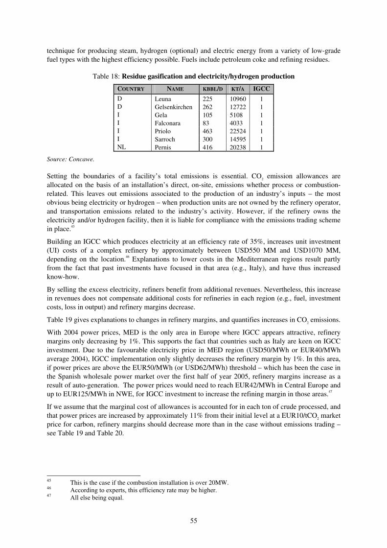
55

technique for producing steam, hydrogen (optional) and electric energy from a variety of low-grade fuel types with the highest efficiency possible. Fuels include petroleum coke and refining residues.

Table 18: Residue gasification and electricity/hydrogen production

COUNTRY NAME KBBL/D KT/A IGCC

D Leuna 225 10960 1 D Gelsenkirchen 262 12722 1 I Gela 105 5108 1 I Falconara 83 4033 1 I Priolo 463 22524 1 I Sarroch 300 14595 1 NL Pernis 416 20238 1

Source: Concawe.

Setting the boundaries of a facility’s total emissions is essential. CO2 emission allowances are allocated on the basis of an installation’s direct, on-site, emissions whether process or combustion-related. This leaves out emissions associated to the production of an industry’s inputs – the most obvious being electricity or hydrogen – when production units are not owned by the refinery operator, and transportation emissions related to the industry’s activity. However, if the refinery owns the electricity and/or hydrogen facility, then it is liable for compliance with the emissions trading scheme in place.45

Building an IGCC which produces electricity at an efficiency rate of 35%, increases unit investment (UI) costs of a complex refinery by approximately between USD550 MM and USD1070 MM, depending on the location.46 Explanations to lower costs in the Mediterranean regions result partly from the fact that past investments have focused in that area (e.g., Italy), and have thus increased know-how.

By selling the excess electricity, refiners benefit from additional revenues. Nevertheless, this increase in revenues does not compensate additional costs for refineries in each region (e.g., fuel, investment costs, loss in output) and refinery margins decrease.

Table 19 gives explanations to changes in refinery margins, and quantifies increases in CO2 emissions.

With 2004 power prices, MED is the only area in Europe where IGCC appears attractive, refinery margins only decreasing by 1%. This supports the fact that countries such as Italy are keen on IGCC investment. Due to the favourable electricity price in MED region (USD50/MWh or EUR40/MWh average 2004), IGCC implementation only slightly decreases the refinery margin by 1%. In this area, if power prices are above the EUR50/MWh (or USD62/MWh) threshold – which has been the case in the Spanish wholesale power market over the first half of year 2005, refinery margins increase as a result of auto-generation. The power prices would need to reach EUR42/MWh in Central Europe and up to EUR125/MWh in NWE, for IGCC investment to increase the refining margin in those areas.47

If we assume that the marginal cost of allowances is accounted for in each ton of crude processed, and that power prices are increased by approximately 11% from their initial level at a EUR10/tCO2 market price for carbon, refinery margins should decrease more than in the case without emissions trading – see Table 19 and Table 20.

45 This is the case if the combustion installation is over 20MW. 46 According to experts, this efficiency rate may be higher. 47 All else being equal.

56

Table 19: Changes in refinery output, margins and CO2 emissions following investment in an IGCC

% CHANGE COMPARED TO CONFIGURATION WITHOUT IGCC

NWE #6 + IGCC

MED #6 + IGCC CEN #6 + IGCC

NWE

PRICES MED

PRICES

Fuel & Loss 23% 5% 49% 49%

Output -8% -7% -12%

AGO -17% 8% 0%

IGO 124% -4% 63%

HFO -100% -100% -100%

Running Expenses 100% 85% 124% 124%

Crude & Feedstock -3% -5% -4% -4%

Fixed Costs 44% 35% 60% 60%

CO2 emissions 17% 15% 62% 62%

Power produced (GWh) 18 694 28 376 16 857

% Power sold to the grid 26% 15% 54%

Net margin no carbon cost -35% -1% -17% -20%

Refinery margins are, however, higher than if only the carbon allowance price was accounted for and not the increase in power prices.

With emissions trading, investments in IGCC technology may be encouraged as refiners would be able to benefit from an increase in the price of the power sold. At a EUR10/tCO2 market price for carbon impacting the cost structure both directly and indirectly, refinery margins would not decrease from a situation where there is no IGCC power plant if power prices rise to EUR160/MWh for the NWE area; EUR72/MWh for MED; and around EUR55/MWh for Central Europe. This supposes that no additional power is sold to the grid.

5.4 PRICES FOR END-PRODUCTS

The ability of refiners across Europe to influence market prices both upstream and downstream of the value chain is constrained by the following factors:

57

Table 20: Changes in refinery margins of a complex refinery with IGCC when direct and indirect impact of CO2 emissions are accounted for

NWE #6 + IGCC

MED #6 + IGCC CEN #6 + IGCC

NWE

PRICES MED

PRICES

Net margin no carbon cost (USD/bbl)

3.34 6.29 4.22 4.26

Net Margin including carbon cost of allowance (% change from IGCC simple)

-19% -10% -22% -22%

Net Margin including carbon cost and pass-through of opportunity cost onto power price

-19% -10% -19% -19%

Crude Pricing

Upstream, the price of crude oil is not an element of competition for European refineries since it is fixed across Europe. Crude oil is sold through a variety of contract arrangements and in spot transactions. Oil is also traded on futures markets but not generally to supply physical volumes of oil, more as a mechanism to distribute risk. These mechanisms play an important role in providing pricing information to markets. Pricing of Physical Crude Oil Trades is generally based on a formula approach where a marker crude is used as the base and then a quality differential as well as a demand/supply (premium/discount) is added depending on the crude being purchased. Thus in times of tight supply this premium will rise and gradually drag up the Marker crude price, whilst in times of surplus supply, a reduced premium or even a discount will drag down the Marker crude price. Of course big changes/announcement/events that can significantly influence crude supply levels will sometimes result in a large step change in the prices of crude (e.g., OPEC announcements; a war; major refinery outages);

The European refinery industry is, thus, assumed to be price-taker on crude oil and several refinery product markets. The main elements on which refiners can lower the costs and influence their margins are the operational costs (e.g., number of operators of a refinery; energy consumed; and maintenance) and the optimisation of the crude slate and finished products pattern.

Downstream

In the downstream market, refinery products are treated as commodities. Prices are set by market operators quoted in specialized energy reviews including the Platt’s and Argus. Contracts for supply of refined products are generally based on these quotations. Prices for refinery margins calculations before/after CO2 emissions limits will be based on Platt’s 2004 average data.

Nevertheless, several European countries are supplied in certain products by European refineries almost exclusively: aviation gasoline, motor gasoline, and fuel oil as indicated in Table 21. It is conceivable that European refineries are price-makers in these markets and would thus have the possibility to pass on most if not all of their CO2 cost to consumers – either the actual cash costs or the full opportunity cost, as witnessed in electricity markets. If this were the case, emissions trading could entail a net earning for the refining industry.

58

Table 21: Share of imports from European countries (2003)

SHARE OF IMPORTS FROM EUROPE LPG NAPHTHA

AVIATION GASOLINE

MOTOR GASOLINE

KEROSENE TYPE JET

FUEL DIESEL OIL FUEL OIL LUBRI-CANT BITUMEN PETRO-

LEUM COKE TOTAL Austria 84% Ni Ni 100% 100% 100% 87% 100% 92% 100% 97% Belgium 97% 80% 100% 99% 51% 89% 92% 89% 91% 11% 86% Czech Rep. 36% 100% 100% 100% 100% 100% 100% 100% 100% 88% 98% Denmark 0% Ni 100% 16% 23% 27% 26% 43% 54% 2% 25% Finland 16% 5% 100% 0% Ni 11% 39% 66% 0% 0% 17% France 37% 51% 100% 77% 16% 49% 18% 86% 88% 33% 46% Germany 79% 80% 100% 95% 100% 86% 71% 90% 97% 55% 85% Greece 38% Ni Ni 58% 7% 14% 0% 100% Ni 7% 20% Hungary 17% 3% 100% 96% Ni 46% 64% 91% 0% Ni 56% Ireland 100% Ni 100% 86% 100% 87% 97% 93% 100% 55% 89% Italy 16% 5% Ni 73% 0% 1% 30% 96% Ni 0% 23% Lux. 100% Ni Ni 100% 100% 100% 100% 100% 100% Ni 100% Netherlands 65% 64% Ni 56% 63% 44% 48% 90% 100% Ni 54% Poland 26% Ni 100% 100% 100% 39% 72% 36% 54% 34% 41% Portugal 83% 74% 100% 100% 19% 89% 80% 100% 100% 5% 62% Slovak Rep. 12% 13% Ni 74% 0% 87% 59% 86% 93% 60% 68% Spain 31% 8% 100% 89% 32% 70% 71% 94% 96% 6% 53% Sweden 44% 21% 67% 78% 84% 33% 79% 19% 98% Ni 53% UK 41% 38% 75% 16% 6% 57% 8% 14% 90% 0% 22% Cyprus 32% Ni Ni 54% 9% 22% 0% 67% 100% 0% 12% Estonia 0% Ni Ni 90% 60% 16% 7% 0% 31% Ni 37% Latvia 22% Ni Ni 72% 97% 14% 4% 33% 13% 0% 28% Lithuania 1% Ni 100% 100% 0% 3% 35% 32% 0% Ni 17%

Source: IEA statistics

Ni: no imports.

59

6. COMPARISON OF CO2 COSTS WITH INVESTMENT COSTS IN DESULPHURISATION

With the threat of CO2 emissions leakage playing an important role in debates over the EU ETS’s impact on emissions and industry, we now explore the possibility of increased competition from foreign producers. The aim of this section is to determine how foreign products could compete with European refinery production. New or increased trade flows as a result of emissions trading are also examined, including specific barriers related to the transport of finished or semi-refined products. In what follows, we consider a full cost accounting of CO2.

A requisite when observing potential changes in refinery products’ trade flows is to distinguish between countries which sell products that comply with European specifications from those for which such compliance is not mandatory. Available extra refinery capacity for trade is also crucial. Utilisation is already high in the main consuming areas in Europe, and throughputs may have to rise significantly in other regions in order to supply products for exports – see Annex 5.

Benefiting from the absence of a CO2 cost, non-carbon constrained refinery producers may increase their supply to the European market. Investments in desulphurisation units may nonetheless be required if we take for example products from the Mediterranean Basin or the Former Soviet Union which do not bear similar environmental specifications.

To illustrate the increase in costs to meet European fuel specifications, we use approximate costs for upgrading Russian refineries with HSK or HSK+FCC configurations. Estimates are based on a capacity calculated by averaging the relevant refineries capacities of these areas.48 They are provided as an ISBL (Inside Battery Limits) calculation and carry a +50/-40% error margin – see Annex 18 for details on AACE Cost Estimate Classification Systems. We assume that foreign products would need to comply with Euro 5 specifications, becoming mandatory as early as 2009.

6.1 INVESTMENT COSTS IN DESULPHURISATION TECHNOLOGIES TO MEET THE EUROPEAN

SPECIFICATIONS

Investment requirements for product-quality improvements are derived from published cost estimates for meeting the European and North-American fuel standards. In practice, the exact cost of improving fuel quality in a region will depend on the interaction between many factors, including existing refinery configurations, crude slates and technological developments in the refinery process (WEIO, 2003).

Production of diesel and gasoline fuels which meet the latest European requirements for sulphur content Euro 4 would only make economic sense to foreign producers that can increase exports and thus compensate for additional expenditures in production of low sulphur fuels. All the former Soviet republics are currently suffering from differences of fuel standards and in this respect, various investment proposals have been implemented by Russia’s major oil companies, illustrated in Table 22.Table 22 Particular care has been given to the production of diesel additives in order to overcome some of the physical and chemical characteristics of Russian gasoil, and to meet European specifications.

48 based on OGJ 2004 data

60

Table 22: Russian construction update

COMPANY AND

LOCATION PROJECT EXPECTED COMPLETION PROJECT NOTES

Alliance Oil Co. - Khabarovsk

Hydrocracker and Hydrotreater

2006 New

Lukoil – Volgograd Hydrotreater and

Isomerization 2010

Second stage for diesel and New

Salavatnefteorgsintez – Salavat

FCC and Hydrotreater 2005 New

Slavneft – Yaroslav Hydrocracker and

Visbreaker 2005 New and Expansion

Source: O&G (2005).

For some Russian refineries, the following differences in fuels specifications are emerging (Table 23). For gasoline products, the main difference between Russian and European specifications is the aromatics content (48 and 35 vol%). Therefore, the actual Russian gasoline pool must be diluted with products with lower aromatic content.

Table 23: Major differences in produced fuels characteristics between Russia and Europe 49

RUSSIA EURO 4

MOTOR GASOLINE UNLEADED 95

Sulphur % 0.029 50 ppm

Lead content max (g/liter) 1.3 0

DIESEL OIL 0.5 0.35

Sulphur % 0.5 50 ppm

Cetane Number 45 51

Tar Content % 19 15

Source: Axens.

Investment costs in desulphurisation units depend on the refinery’s complexity. Two cases are considered in depth in this section: Russian hydro-skimming installations, and more complex fluid catalytic cracking installations.

49 Note that some Russian refineries produce gasoil with low sulphur tenure (i.e.,50ppm).

61

6.1.1 Upgrading hydro-skimming refineries

In a hydro-skimming configuration, the gasoline pool is basically composed of reformate and straight-run light gasoline, with respective aromatic contents of about 70 and <1 vol%. Partly because of its poor RON (75), straight-run gasoline amount added in the gasoline pool is limited. One solution is to process the light gasoline in an isomerization unit that produces an isomerate with no aromatics and an RON of 84.

Table 38 of Annex 16 shows that to meet the European specifications for a Russian hydroskimmer, the isomerization capacity is more than nine-times increased: the Russian refining industry is critically lacking this type of process unit at the moment. To meet European specifications, hydrotreatment is also multiplied by four, mainly used for the diesel pool to reach the 10 ppm specification. Alkylation cannot be used in a hydroskimming configuration because there is no olefin feedstock available. The reforming and isomerization units treat all the naphtha available. At the end, however, the aromatic content is still a bit high and the RON a bit low. Adjustments are made by adding some MTBE. Since MTBE is expensive, processing naphtha in isomerization is chosen before using MTBE.

The required investments are focused on gasoline and diesel pools. Table 24 gives the cost breakdown of investments need to upgrade a Russian hydroskimmer. Only product qualities upgrading such as isomerization, reforming, etc. have been considered, and no incremental conversion has been added.

Table 24: Required capacities and investments for Euro 5 specification – Russian HSK

INSTALLED PROCESSING CAPACITIES &

UTILISATION RATE EURO 10 PPM – RUSSIAN

SPECIFICTIONS OSBL 106

USD 50

Crude Purchases kt/yr 7 017 7 017

TYPE OF PROCESS PROCESS KT/YR 136

Upgrading Isomerization 311 48

Hydrotreating Kero-GO HDS 877 80

Others Sulphur Recovery 8 9

Source: Axens.

In order to best assess the required investment and not to benefit from any scale effect when looking at a group of 7 refineries, the total processing capacity has been divided by 7 in order to obtain an average of 7 MTPA. For such a refinery, the total investment adds to USD 136 106.51 This equals a USD 19.4 per tonne or a USD 2.65 investment cost per barrel, considering that the Urals specific gravity is 0.86.

50 The total costs incorporate all of the elements included in real life projects. These include all of the front-end costs of process selection, engineering, and project management, and all the on-plot facilities including catalysts, the associated off-plot and other infrastructure investments required including amounts for all the associated facilities to ensure the project does not impair the chances of other future investments. 51 This means that for the whole Western part of Russia, HSK refineries would need to invest a total of 952 106 USD in order to achieve gasoline and diesel products similar to Euro V.

62

6.1.2 HSK + FCC configuration

The gasoline constraint on aromatic content is the same as in the hydroskimming configuration. If we assume that the upgrade of product qualities is not made by investing in conversion units, gasoline must be treated in a selective hydrotreatment unit to meet the 10 ppm specification. Table 39 in Annex 16 illustrates the changes in the process units needed for Russian FCC refineries to meet Euro V specifications, and Table 25 gives the cost breakdown.

To best assess the cost of the required investments, again, the total processing capacity has been divided by 8 to obtain an average capacity of 9 MTPA. For such a refinery, the total investment adds up to 252 106 USD.52 This represents an additional cost of 28 USD per ton or 3.83 USD per barrel.

Table 25: Required capacities and investments for Euro 5 specification production – Russian HSK + FCC


UTILISATION RATE EURO 10 PPM – RUSSIAN

SPECIFICTIONS OSBL 106

USD

Number of refineries 1 1


TYPE OF PROCESS PROCESS KT/YR 136

Upgrading Isomerization 306 47

Reforming 201 44

Hydrotreating FCC Naphtha HDT 264 28

Kero-GO HDS 1 530 118


Source: Axens

Comparatively, if CO2 prices reach EUR30/tCO2, the additional cost of CO2 borne by European refineries range between USD 1.02/bbl for a hydroskimming configuration to USD 1.87/bbl for a FCC+HCU installation in NWE. The additional CO2 cost is lower than the investment costs incurred by a Russian refiner for compliance with European specifications, if it were to consider exporting to Europe. Knowing that our CO2 cost assumptions are based on a full cost accounting, thus very much on the high side, the risk of rampant CO2 leakage from a cap on European oil refineries appears limited. Note, however, that European refiners are not the only players that might consider installing just outside the European Union. Domestic margins in non-EU countries could justify supplemental capacity at lower unitary investment cost for export purposes.

Moreover, as we will see in 6.2, even if it were economic to invest in upgrading the quality of Russian fuel products, at present several factors limit the possibilities to export clean products (e.g., gasoline and diesel fuels) in any EU country, among which freight costs. The freight cost for diesel and gasoline is much higher than that of crude oil freight (see ANNEX 21).

52 This means that for the whole Western part of Russia, HSK + FCC refineries would need to invest a total of 2.016 billion USD to achieve gasoline and diesel products quality similar to Euro V.

63

6.2 POLITICAL QUESTIONS

Political, macro-economical and security of supply considerations are likely to play an important role in the decision of an oil producing country to enter the market for finished products. European companies investing in non-European countries may be constrained by political or technical factors.

EU and non-EU operators already own important energy assets outside EU and are involved in joint venture operations with oil producing countries. They also have significant links through interests in oil production and port activities. Thus, preventing upgrade investments on political reasons may not be likely. Rather, economic justifications should be the driver for investment decisions.

6.3 EXTRA AVAILABLE CAPACITY TO MEET INCREASED EXPORTS - CONSTRUCTION OR EXPANSION OF

REFINERIES OUTSIDE OF EUROPE

The amount of additional refined products imported into Europe is limited by the extra capacity available to foreign refineries to meet European demand and quality specifications. Figure 16 shows the global investment in refinery upgrades to meet environmental specifications over the last decade. Europe’s current refining capacity approaches 15 mbbl/d whereas more than 40 mbbl/d of capacity is now equipped with hydro-treatment equipment used to improve the environmental quality of refined products.

Figure 16: Global upgrading unit capacity

0

5

10

15

20

25

30

35

40

45

1986

1987

1988

1989

1990

1991

1992

1993

1994

1995

1996

1997

1998

1999

2000

2001

2002

2003

2004

mill

ions

bbl

/d

VDU Coking

Cat. Cracking Reforming

Hydrocracking Hydrotreating

Source: Oil & Gas Journal

On the other hand, the rapid growth in clean product is putting pressure on upgrading capacity; the implication is that more distillation and above all more upgrading capacity is needed. Upgrading capacity is growing by less than 1.7% per year while demand for clean products is growing by 2%. The installation of units for upgrading seems to be stagnant – see Figure 17.

The ever increasing regulatory demand for cleaner fuels is also contributing to tighter refining capacities. While technology and process are certainly available to ultimately achieve this objective with substantial investments, the production of such cleaner fuels can easily reduce the resulting finished product slate by 5-6% of crude oil input as more energy is spent in refining – and more CO2 emitted as a result.

64

Figure 17: Global upgrading capacity: historical evolution and forecast

0,381,05

1,49

21,16

1,88 2,032,74

1,31 1,071,46

0,780,06 0,28

0,97 0,651,06 1,01

1,480,90

2,66

-2,71

0,781,160,340,08

0,961,841,35

-3,50

1,713,632,732,56

28,48

2,001,420,523,63

1,131,671,051,25

-4

-2

0

2

4

6

8

10

1987

1988

1989

1990

1991

1992

1993

1994

1995

1996

1997

1998

1999

2000

2001

2002

2003

2004

2005

2006

2007

millio

ns b

bl/d

-10

-5

0

5

10

15

20

25

30

35

%

Upgrading Capacity Growth excluding HydrotreatingUpgrading Capacity Growth (excl. Hydrotreating) as percentage of the World Refining Capacity (right)

Projections

Source: Oil & Gas Journal and HETCO

Projections

Source: Merino, 2005.

According to the World Energy Outlook, the bulk of future refinery investment will occur in the Middle East and Africa – see Annex 14. Part of the investments will also take place in Asia in response to the region’s strong growth in demand for refined products, particularly in China and in India. These investments will mainly be greenfield projects of simple refineries or semi-complex facilities, far from the European or North-American facilities in terms of environmental requirements. They will also serve essentially the local markets. Asian and Middle Eastern products are therefore unlikely to undermine the European markets, even though the European refinery industry faces both a CO2 constraint.

65

7. CONSEQUENCES ON TRADE FLOWS: A RE-DISTRIBUTION OF LOCATIONS OR A CHANGE IN PRODUCTION STRATEGIES?

In this section, we assess the potential increase of import penetration on the European market as a result of CO2 costs. Evaluation is also made on whether the introduction of a CO2 price may entail a change in product yields and whether the crude oil feedstock of European refineries may be modified.

The main refined products imported into Europe – including intra-European trade – are diesel (35% of total refined products’ imports or 95 626 thousand metric tonnes) and residual fuel oil (18% of total refined products’ imports or 48 294 thousand metric tonnes). We therefore focus on imports of diesel and residual fuel oil, the latter being used as a feedstock for refinery products.

7.1 INCREASE OF FOREIGN IMPORTS INTO EUROPE

According to experts, Mediterranean Basin or Eastern Europe refiners must reach sulphur levels below European standards if they wish to export into the EU: transporting refined products through bunkers or pipelines often adds sulphur to the transported product, as neither vessels nor pipes can be cleaned after each use. Their sulphur specification must therefore surpass European standards and our estimates of investment in desulphurisation may be on the low end of actual costs, if refiners were to consider such strategy.

Overall, imports should not increase as a result of the additional cost of the CO2 cap. First, the additional costs that foreign refiners may incur to enter the European market (e.g.,, clean freight rates, stringent product specifications) probably influences their downstream strategies (i.e.,, choice of market they wish to supply) more than an increase in cost for European refineries.53

Second, as explained in 5.4, several European countries are almost exclusively supplied by European refineries for certain products, e.g., aviation gasoline, kerosene, etc. If European refineries are price-makers for these products, they may have the possibility to pass on most, if not all, of their CO2 cost to consumers – thus encouraging foreign competition.

7.2 CHANGE IN PRODUCTION STRATEGY

If a European refinery has excess allowances, emissions trading will not require a change in production pattern. If, however, it needs to purchase allowances, an arbitrage might be made between paying for allowances and changing production patterns to reduce CO2 emissions. In theory, options include producing less-CO2 intensive products; limiting overall output; and changing the crude mix to lighter and sweeter inputs for products destined to the European market.54 The following section considers the possibility to import sweeter and pre-refined products as feedstock.

European refineries may choose to produce less CO2 intensive products. Although results in Table 9 must be interpreted with great care before making any firm conclusions, gasoline production is more energy-intensive than diesel production in terms of global production. Thus, European refiners may focus their production pattern on diesel production, adjusting their feedstock and configuration accordingly. Such adjustment may only be feasible at the margin.

Would European refineries alter their location strategy if CO2 prices reached much higher levels? In the cement industry, the carbon intensive part of production may be shifted to non-constrained countries. Oil industry experts see such option as extremely unlikely for the refinery industry, due to operational and logistical problems of moving intermediate products from one refinery to the next.

53 If foreign refineries are already conforming to European specifications (i.e., desulphurisation investment costs were already undertaken), then the arbitrage may be limited to the comparison between the additional cost of freight and the CO2 cost increase. 54 For example, multinational groups maybe able to incorporate the carbon factor in their feedstock decisions – optimising their inputs.

66

7.3 CHANGE IN CRUDE OIL FEEDSTOCK

This part investigates the consequences of treating Russian fuel oil (M-100 type) in European refineries, as a means to reduce CO2 emissions. Configuration 2 (HSK + VB + FCC) is chosen of NWE refining capacities because it represents close to 25% of Europe’s total refining capacity. We assume that the refinery processes 10% of M-100 (see Annex 15 for details).55

Table 26 illustrates the change in production pattern following a 10% input of M-100 HFO in the refinery feedstock.

Table 26: HSK + VB + FCC refinery mass balance, M-100 processing

NORTH WEST EUROPE 2-HSK+VB+FCC 2-HSK+VB+FCC + M100

Number of Refineries 21 21

Kt Kt

Input 157 398 173 819

Output 139 974 or 89% 154 935 or 89%

LPG 3 207 or 2% 3 535 or 2%

Propane CIF 3 158 or 2% 3,535 or 2%

Butane CIF 49 0

Naphtha FOB 11 757 or 7% 11 803 or 7%

Gasoline 45 310 or 29% 49 070 or 28%

Eurosuper 95 FOB 24 917 or 16% 29,100 or 17%

Premium 98 FOB 1 434 or 1% 1,434 or 1%

Export (US / 92) FOB 18 959 or 12% 18,536 or 11%

Jet A1 CIF 10 099 or 6% 10 099 or 6%

AGO CIF 38 057 or 24% 38 057 or 22%

IGO CIF 12 855 or 8% 12 519 or 7%

HFO 15 187 or 10% 24 948 or 14%

LS HFO FOB 0 0

HS HFO FOB 0 24,948 or 14%

LS Bunker FOB 15 187 or 10% 0

HS Bunker FOB 0 0

Bitumen 2 989 or 2% 4 268 or 2%

Sulfur FOB 513 636

Coke 0 0

Fuel and loss 17 424 18 883

Source: IEA, Axens

As illustrated in Table 27, overall, CO2 emissions increase due to the higher amount of feedstock processed in the refineries, but the CO2 produced by ton of feedstock decreases. This is due to the SO2 constraint imposed on refineries (e.g., Large Combustion Plant Directive). To limit the SO2 emissions, there is a limit on the sulphur content of the refinery fuel. However, as the M-100 has a higher sulphur content than the initial AR (2.58 versus 1.40wt %), it is not possible to produce the 1.5 wt% sulphur content fuel oil (low sulphur bunker) anymore. The fuel oil produced is then high sulphur HFO (2.5 wt% sulphur content).56 As a result, the refinery needs to import more natural gas to compensate the

55 M-100 quality was taken as “straight run”, by opposition to the “cracked” quality which would be much more difficult to process and crack in the refinery. A price difference of about 20 USD/t is typically observed between these two qualities of fuel oil M-100. The name M-100 is used for all the three different specifications on sulphur content (<1%wt, <2%wt, >2%wt). In this study, the highest fuel specification was chosen as it corresponds to the one produced on a 100% Urals feedstock. 56 To avoid this phenomenon, segregating M-100 import would be required, but as mentioned earlier, this requires suitable storage capacities and operating flexibility.

67

decrease in fuel oil consumption. The share of natural gas in refinery fuel increases by 5%. As the carbon content of the natural gas is lower than for heavy fuel, the refinery fuel in the M-100 case emits less CO2 when it is burnt.

Hydrogen consumption increases by 12% due to the higher amount of feedstock processed in the hydro-treating units. It is assumed that this required amount of H2 is available in the refineries, otherwise, refiners would not import M-100 or would treat less crude.

Table 27: HSK + VB + FCC refinery margins, M-100 processing

NORTH WEST EUROPE

2- +VB+FCC57 2- +VB+FCC

+M100

Crude & Feedstock cost USD / t 309.90 298.44 Gross Products Worth * USD / t 369.64 357.19 Fuel & Loss USD / t 18.48 18.15 Gross margin USD / t 59.74 58.75 Variable Costs USD / t 0.70 0.69 Catalysts & Chemicals USD / t 0.70 0.69 Fixed Costs USD / t 15.01 14.57 Personnel USD / t 1.88 1.82 Maintenance USD / t 7.51 7.28 Overheads USD / t 3.75 3.64 Insurance USD / t 1.88 1.82 Working Capital USD / t 0.00 0.00 Running Expenses USD / t 15.71 15.26 Net margin USD / t 25.55 25.35 SG 0.8445 0.8553

Net margin USD / bbl 3.43 3.45

CO2 emissions kt 50,908 54,589

CO2 emissions t / t crude 0.338 0.329

Source: IEA, Axens

* Fuel and loss is a component of the GPW. Thus, it cancels out in the Gross Margin.

The price of M-100 for a NWE refiner is based on the Petroleum Argus price January 22, 2003. At that time, the differential with HFO 3.5% was 14 USD/t. In 2004, the average NWE CIF price for heavy fuel oil 3.5% was 150 USD. Thus, using the same differential than in 2003, an M-100 NWE CIF price was estimated to reach 164 USD/t.

Table 27 highlights the change in refinery margins following the import of M-100 in the feedstock. The net margin per ton of product of the case including M-100 is slightly higher than the net margin of the configuration without M-100 imports. As the price of M-100 is lower than a crude price, the crude and feedstock cost per tonne is lower than with M-100. As recalled above, in the finished products pattern, the heavy fuel oil takes part of the share of distillate products: the refineries produce 0.1 t of heavy fuel oil per ton of crude against 0.15 t with M-100 processed. Since the HFO is less valuable, the gross products worth (GPW) decreases. Moreover, HFO prices are below the M-100, which means that lower feedstock cost will not make up for the GPW loss.

The running expenses are lower when M-100 is processed. This is mainly due to the fact that the fixed costs are related to the value of a new equivalent refinery in the calculations: an increase of 10% of

57 This case is different from the configuration #2 NWE illustrated before. The reason lies in the import of MTBE in the previous case as opposed to import of methanol to produce MTBE in the present case.

68

the feedstock does not lead to an increase of 10% of investments – about 7% in this case – because of scaling effects. Thus, investments costs per ton of feedstock are lower when M-100 is processed, and so are the fixed costs. This decrease of costs covers the loss in Gross Margin.

The difference between the two margins is very low, and is sensitive to the assumptions. For example, if the price of M-100 reached 165USD/t, the refining margin would be equal in both cases. With a price below that level, the M-100 case would become more attractive to process than crude oil. Therefore, fuel oil processing is extremely sensitive to its procurement price. The benefits related to this opportunity need to be assessed on a case by case basis with the refinery’s précised economic environment and process configuration.

If the same refinery configuration was to process only M-100, the refinery margin would reach 3.65USD/t. In reality, it is impossible to treat 100% of M-100 because there would not be enough light products to meet the final products specifications and demand. These calculations are reliable for treating around 10% of M-100, as a marginal feedstock of the refinery, but not as core material. To estimate the margin for processing around 50% of M-100, additional simulation would be necessary as it would lead to different results (e.g., heavier final products pattern, different running expenses, etc.).

The competitiveness of both cases does not change once a CO2 price is introduced. Emissions are lower per ton of crude with M-100 imports. Thus, although emissions trading is not the main driver of an increase in trade flows for Russian M-100 imports, imports should increase as a result of the introduction of emissions trading. This may be even more realistic if low sulphur M-100 is imported.

69

8. EURO 5 STANDARDS FOR EUROPEAN REFINERY PRODUCTS: IMPACTS ON INVESTMENTS AND EMISSIONS

The EU is preparing to impose stricter emissions limits on diesel vehicles – see Table 35 and Annex 10, in particular for nitrogen oxides (NOx) and particulate matter (ppm) which pose the most serious health problems. With the next generation standards for diesel cars (known as Euro 5) currently under preparation for 2010,58 some member states including France and Germany have already started to press ahead with measures of their own. For this reason, a case with products complying with Euro 5 standards is also modelled. The configuration 2 (HSK+VB+FCC) is chosen because it represents 55% of the North West Europe refining. Only future specifications are considered, and the demand pattern remains the same.

In order to reach the 10 ppm sulphur specification, industry states that complex refineries converting heavier products or crude oils may face the most difficult technical and economical challenges in coping with new product specifications. The main requirement is to increase the severity of hydrotreatment units for gasoline and diesel. In the 50 ppmwt case, most of the FCC naphtha is blended in the export grade because of its high sulphur content. This is due to the limited capacity of FCC naphtha hydrotreating (HDT). In order to avoid losing valuable FCC naphtha to the export high sulphur gasoline market, investments are made in FCC naphtha HDT to make more valuable products.

If we consider that the investment cost for FCC naphtha HDT reaches 27 MMUSD for one refinery, this equates in an increase in production costs by 3.76 USD/t or 0.5 USD/bbl – see Table 28 for investments required. Moreover, as more sulphur will be recovered from the HDT unit, sulphur recovery capacity will need to be increased.

A marginal increase of CO2 emissions of 1.1% occurs if products’ specification is more stringent. 0.40% is due to the increased capacity of naphtha FCC HDT. The other 0.70% comes from a slight change in refinery fuel composition. In the 10 ppm case, the additional hydrogen that is required in gasoil HDS to reach the 10 ppm sulphur content is retrieved from the in the refinery fuel composition of the 50 ppm case.59 The hydrogen removed from the refinery fuel is hence replaced by products that have higher carbon content, and therefore release more CO2.

The raise of naphtha FCC HDT capacity represents about 15% of the total hydrogen consumption increase between 50 and 10 ppm specifications. The remaining 85% are due to more severe operating conditions of kerosene and gasoil HDS – see Table 29 for details on H2 consumption increase.

58 The Commission is expected to present its proposal for Euro 5 in autumn 2005. 59 The increase in H2 consumption in the GO HDS is generally estimated around 10-15%. Here, we have considered the least favourable conditions with an increase by 30% in order to penalise the model in terms of CO2 emissions.

70

Table 28: Required capacity investments to reach Euro V specifications – North West Europe HSK+FCC+VB configuration

REQUIRED CAPACITIES AND INVESTMENTS +VB+FCC

EURO 50 PPM

+VB+FCC EURO 10 PPM

EURO 10 -

EURO 50 PPM

EURO 10 - EURO 50

PPM

OSBL MMUSD

Number of Refineries 21 21 21 1 1

Crude purchases kt/yr 150 809 150 809 150 809 7 181 7 181 Type of Process Process kt/yr % kt/yr % kt/yr kt/yr 29 Crude Distillation Atm. Distillation 173 681 87% 173 681 87% 0 0 0 Vacuum Distillation 73 993 74% 73 993 74% 0 0 0 Conversion FCC 41 980 92% 41 980 92% 0 0 0 Hydrocraking 0 0 0 0 0 Visbreaking 12 508 99% 12 508 99% 0 0 0 Coking 0 0 0 0 0 Residue Cracking 4 632 96% 4 632 96% 0 0 0 Upgrading Isomerisation 6 888 115% 6 890 115% 2 0 0 Reforming 26 169 100% 26 169 100% 0 0 0 Alkylation 3 638 99% 3 638 99% 0 0 0 Oxygenate Production MTBE 487 99% 487 99% 0 0 0 Hydrotreating (HDT) SR Naphtha HDT 53 488 62% 53 488 62% 0 0 0 FCC Naphtha HDT 191 96% 5 452 2854% 5 261 251 27 Hydro-desulphurisation (HDS) Kero-GO HDS 41 322 128% 40 938 127% -384 0 0 VGO HDS 4 487 100% 4 487 100% 0 0 0 Hydrogen Production H2 Plant (Steam Ref.) 0 0 0 0 0

Others Sulphur Recovery 513 522 9 0 1

71

Table 29: HSK+VB+FCC hydrogen mass balance

H2 consumption 50 ppm 10 ppm 10 - 50 ppm

kt t/t feed kt t/t feed D t/t feed

Atmospheric Residue Desulphurisation 57.8 1.30% 57.8 1.30% 0%

FCC pretreatment 49.6 1.11% 49.6 1.11% 0%

Naphtha FCC HDT 0.3 0.15% 8.2 0.15% 0%

Naphtha HDT 36.1 0.11% 36.1 0.11% 0%

Benzene hydrogenation 97.7 0.44% 97.8 0.44% 0%

ISO 24.0 0.35% 24.0 0.35% 0%

Kero HDS 1.2 0.03% 1.2 0.03% 5%

GO HDS 138.7 0.34% 178.3 0.44% 30%

Total 405.3 452.9

As focus was placed on the specification change only, the production pattern of the model is remained unchanged - and so is the gross products worth (GPW). Only utility and catalysts consumption impact the refinery margin. The new refinery margin is slightly lower than in the 50 ppm case. It decreases by 0.1 USD/bbl.

73

CONCLUSION

Companies’ perception of the cost of CO2 in a long-term perspective is crucial to understand how emissions trading will eventually affect refiners’ investment decisions. The above analysis of the impacts of a CO2 cost on EU refiners hinges on a number of assumptions, the most important one being the treatment of the cost by refiners themselves. Treating EU ETS allocations on a cash cost basis, rather than a full opportunity cost basis, can be criticised as a narrow, short-term perspective. On the other hand, the EU ETS does not envision a full auctioning of allowances before long (only a maximum of 10% may be sold to installations in 2008-2012), and most plans include reserves of allowances for new entrants – a de facto subsidy in this carbon-constrained environment. Under such circumstances, it is not clear how incentives to invest outside the EU differ now, from what they were prior to the CO2 constraint.

This said, the CO2 constraint introduced in the EU affects costs beyond those triggered by installations’ caps:

CO2 emissions for a refinery vary with its fuel consumption. Refineries may decide to increase their use of natural gas, instead of heavy fuel oil, in an attempt to lower overall CO2 emissions. This may increase gas prices, with repercussions on other consuming sectors. However, this effect could be mitigated by a growing price differential between natural gas and heavy fuel oil, at the advantage of the latter – not unlike what is happening now in the power generation sector where generators burning coal cover emissions with CO2 allowances instead of switching massively to cleaner, yet more expensive, natural gas. We have not considered the full repercussions of such a scenario.

The rise of electricity prices will affect refineries that purchase electricity from the grid. The current market structure in Europe and the practice of marginal cost pricing in power generation should lead to the pass through of the carbon opportunity cost to wholesale markets. There are good theoretical reasons to believe that CO2 prices should not be fully passed-through under the EU emissions trading scheme, such as a repetitive allocation process that somewhat discourages mitigation, the degree of competition in the power market, and the treatment of new entrants. The pricing behaviour of generators has yet to be explored in light of these considerations.

European environmental specifications are pushing for more CO2-intensive refining processes, exacerbating the impact of the CO2 price if not reflected in the initial allocation. Different treatments across EU countries could affect refiners’ competitiveness from one country to the next.

From the standpoint of international cost competitiveness, amortising any CO2 cost should be evaluated in a current pricing environment of strong demand for refinery products in high growth regions (China, Asia, and North America), with insufficient refining capacity. In the near term, the moderate cash cost imposed by the CO2 cap is unlikely to represent an obstacle to European gasoline exports to foreign markets, especially North America, where demand is strong.

Last, several European countries are supplied in certain products by European refineries almost exclusively; e.g.,, aviation gasoline, kerosene, etc. It is conceivable that European refineries are main players in these markets and thus have the possibility to pass on their CO2 cost to consumers –and, why not, the full opportunity cost, triggering additional profits, as witnessed in electricity markets. In the light of this possibility, developments in refinery product prices must be monitoredto assess its actual cost impact on the refinery industry.

75

REFERENCES

ABN AMRO (2004), Refining – Dawn of a New Era, Fuel Economy, January

Ahman, Markus, Dallas Burtraw, Joseph Kruger, Lars Zetterberg, 2005, The Ten-Year Rule: Allocation of Emission Allowances in the EU Emission Trading System, June 2005, Discussion Paper 05-30. Resources for the Future, Washington DC, www.rff.org

American Petroleum Institute (2002), “Emissions estimating and reporting”, paper presented at the 2nd API Conference on Voluntary actions by the oil and gas industry to address climate change, Houston, Texas, USA, 20-21 November.

Babusiaux, D. (2003), “Allocation of the CO2 and Pollutant Emissions of a Refinery to Petroleum Finished Products”, Oil and Gas Science Technology, Vol 58, No. 6, pp. 685-692.

Clarke, S.C., (2003), “CO2 management – a refiners perspective” www.nrcan.gc.ca/es/etb/cetc/combustion/co2trm/htmldocs/technical_reports_e.html.

Deutsche Bank (2002), “Refining Basics Cracking the European Code”, Global Oil & Gas, March.

Ellerman, D., Joskow, P. and Harrison Jr. D, 2003. Emissions Trading in the US – Experience, lessons and considerations from greenhouse gases; prepared for the PEW Centre on Global Climate Change.

Energy Intelligence, Oil Market Intelligence, April.

EU Joint Research Center, Concawe and Eucar (2003), Well-to-Wheels analysis of future automotive fuels and powertrains in the European context, WELL-TO-TANK (WTT) Version 1 & Appendices 1 to 3, December.

European Commission (2003), “Integrated Pollution Prevention and Control (IPPC) Reference Document on Best Available Techniques for Mineral Oil and Gas Refineries”, February.

IEA, Oil Market Report.

IEA (2005): Act Locally, Trade Globally – Emissions Trading for Climate Policy, International Energy Agency, Paris.

IEA, (2005, forthcoming), Wold Energy Outlook.

IEA Workshop, “8th Energy Experts’ Meeting”, Monday, 6 and Tuesday, 7 June 2005 International Energy Agency - Paris, France

IEA, 2003. World Energy Investment Outlook, OECD/IEA, Paris

IEA, 2001. International Emissions Trading – From Concept to Reality, OECD/IEA, Paris

IFP (2005): Panorama 2005 – a look at…, Rueil-Malmaison, France.

76

IFP (2004): Panorama 2004 – a look at…, Rueil-Malmaison, France.

Maples, R. (1993), Petroleum Refinery Economics, PennWell Books, Tulsa, OK, US.

Merino, A. (2005), Identifying Crude Quality Availability, The Outlook for Refining, International Energy Agency, Eighth Meeting of Experts from Energy Exporting and Importing Countries, June.

Neuhoff, Karsten, Michael Grubb, Kim Keats (2005), “Emission allowance allocation and the effects of updating”, Mimeo, Faculty of Economics, University of Cambridge, UK.

O’Brian, J. and Jensen, S. (2005), “A New Proxy for Coking Margins – Forget the Crack Spread”, NPRA, San Fransisco, March.

Oil and Gas Journal, (2005), Worldwide Construction Update, April 25.

Oil and Gas Journal (2003), 2004 O&GJ Worldwide Refining Survey, Oil & Gas Journal December 22.

Platt’s (1999): Platt’s Guide to Petroleum Specifications, Standard & Poor’s

Reinaud, Julia, 2005. Industrial Competitiveness under the European Union Emissions Trading Scheme, IEA Information Paper, IEA, Paris.

Reinaud, Julia, 2003. Emissions Trading and its Possible Impacts on Investments in the Power Sector, IEA Information Paper, IEA, Paris.

Rolin, O., Quirion, P. (2003), “L'impact du futur marché de quotas d’émission de gaz à effet de serre sur la compétitivité de l’industrie européenne du raffinage”, CIRED (CNRS/EHESS).

Sijm, J.P., Bakker, S.J., Chen, Y., Harmsen, H.W., Lise, W. (2005) : CO2 price dynamics: The implications of EU emissions trading for the price of electricity, Energy Research Center of the Netherlands, September.

Simmonds, M., Hurst, P., Wilkinson, M.B., Watt, C., and Roberts, C.A (2003), “A study of a very large scale post-combustion CO2 capture at a refinery & petrochemical complex”, www.co2captureproject.org/news/documents

SSY Consultancy & Research Ltd. (2005): World Oil Tanker Trends, Volume 1.

77

GLOSSARY

API GRAVITY An scale expressing the gravity or density of liquid oil products devised jointly by the American Petroleum Institute and the United States National Bureau of Standards. The measuring scale is calibrated in terms of degrees API gravity.

ATMOSPHERIC DISTILLATION

The distillation of crude oil under pressure, slightly higher than atmospheric. This is the basic process that takes place in oil refining.

CATALYTIC REFORMING The conversion of naphtha into higher octane intermediate products suitable for blending into finished gasoline.

CHARTER The lease of a ship, for anything from a single voyage to a fixed period of time.

CRACKING The thermal or catalytic conversion of heavier and more complex hydrocarbons into lighter products and coke thus increasing the yield of lighter products from crude oil.

CUTTERSTOCK Distillates of petroleum that are added to asphalt for keeping it liquid at lower temperatures.

DISTILLATION Method of fractionation. Distillation is based on the difference in boiling point of the liquids in the mixture to be separated. Successive vaporisation and condensation of crude oil in a fractioning column will separate out the lighter fractions, leaving a residue.

FCC (FLUID CATALYTIC CRACKING)

Catalytic conversion of heavier and more complex hydrocarbons into lighter products and coke in fluidised bed catalytic reactor with continuous catalyst regeneration. Thus the lighter products yield from crude oil is increased.

HYDROCRACKING Catalytic cracking of hydrocarbon feedstocks in the presence of hydrogen.

HYDRODESULPHURISATION

The process of converting any type of organic sulphur compound into hydrogen sulphide and hydrocarbons in order to reduce the sulphur content of petroleum products complying with the required fuel specifications (includes gas oil and kerosene desulphurisation).

HYDROSKIMMING REFINERY

A refinery with a configuration which only includes distillation, reforming, some hydrotreating, and occasionally sulphur recovery processes.

HYDROTREATING The process whereby feedstocks are place into contact with hydrogen, under high pressure and at a high temperature, in the presence of a catalyst, to reduce the content of sulphur, nitrogen, metals, polyaromatics and olefins.

ISOMERISATION The rearrangement of the molecular structure of hydrocarbons without adding or removing anything from the original material. Isomerisation is used in a refinery to manipulate physical quantities of a substance e.g.,, light naphtha isomerisation is a refinery process used to increase the octane number of naphtha.

KEROSENE A medium – light fraction in between gas oil and naphtha; used for lighting, heating and as fuel for jet and turbo-propeller aircraft engines.

LPG (LIQUEFIED LPG consists of propane and butane which may be wholly or partially liquefied under pressure in order to facilitate transport and storage. LPG

78

PETROLEUM GAS) can be used for cooking or heating or as an automobile fuel.

NAPHTHA A range of distillates lighter that kerosene; used as feedstock for motor gasoline production and in the petrochemicals industry (e.g.,, ethylene and solvents manufacture).

REFINING MARGINS The difference in value between the products produced by a refinery and the value of the crude oil used to produce them. Refining margins will thus vary from refinery to refinery and depend on the price and characteristics of the crude used.

SEMI – REGENERATIVE CATALYTIC REFORMER

A unit in which the regeneration applied in the fixed-bed catalytic reforming process involves periodic shut downs to burn off coke deposited on the catalyst and to recondition the catalyst.

SPOT FREIGHT RATES They apply to the carriage of a single cargo from one specified port to another in the immediate future. They typically include all expenses of operating the vessel, from fuel to crew, exclude costs related to the cargo.

TANKERS They are cargo ships fitted with tanks for carrying liquid in bulk. They may be characterised by their generation or age, their condition, the nature of the cargo they are designed to carry, the trade(s) and/or routes in which they normally operate, the maximum tonnage they can carry, their dimensions or operating limits, etc. Tankers or barges carrying crude oil or heavy persistent petroleum products (heavy fuel oil, for example) are called ‘dirty’ vessels. Gasoline, distillates and other light petroleum products must be carried in smaller, more expensive ‘clean’ product tankers or barges. Aframax ships can carry from 75,000 to 119,999 deadweight tonnes (can go to New York port); Suezmax tankers from 120,000 to 199,999 deadweight tonnes (can go through Suez Canal through fully laden); and VLCCs 200,000 deadweight tonnes or more.

TOPPING REFINERY A refinery consisting only of an atmospheric distillation unit.

VACUUM DISTILLATION Distillation under reduced pressure (less than atmospheric) which lowers the boiling points of the liquid mixture being distilled. This technique, involving a relatively lower temperature, prevents cracking or decomposition of the very heavy hydrocarbon stocks which normally boil at very high temperatures.

VACUUM GAS OIL (VGO) The top product of the vacuum distillation unit.

VISBREAKER A process unit whereby residue feedstock (e.g.,, vacuum gas oil and straight rum atmospheric residue) is heated until it reaches a temperature at which it thermally cracks with a consequent reduction in viscosity and pour point (producing gas, gasoline and gas oil).

Naphtha = charge de reformer pour produire gasoline (after blending)

Between Gasoil and HFO, Vacuum Gas Oil (VGO = in France, Distillates =\ US definition distillates = gasoil\Kero)

79

ANNEX 1: REFINERY PRODUCTS

Refinery fuel gas: Refineries use the C1/C2 fraction as a refinery gas to cover part or most of their fuel requirements. Refinery gas can also contain H2.

LPG: Sometimes C3 and C4 components are also used for refinery fuel, but most of the components will be sold as liquefied petroleum gas (LPG). It’s economically more interesting to sell those to the market. FCCU produces certain categories of C3/C4 (propylene and butylenes) that can be used either for petrochemical plants or as feedstock to octane booster units (Alkylation, Isomerisation) within the refinery. They price higher than regular C3/C4.

Naphtha: Naphtha is the raw gasoline range fraction from crude oil distillation and for petrochemicals.

Gasoline: Gasoline, the fuel for motor cars and light aircraft, represents the highest volume and one of the more valuable refinery products. Automotive gasoline, which is by far the most important gasoline type, consists of a complex mixture of hydrocarbons ranging from C4 to C10. Most refiners produce gasoline in three or four octane grades.

Jet fuel (kerosene, avtur)

Diesel oil / heating oil / gasoil: Diesel fuels are produced by blending of kero and gas oil fractions from the crude distillation unit and gas oil fractions of the high vacuum unit and from conversion units. An upgraded and flexible processing scheme for desulphurisation of blending components is necessary in most refineries in order to arrive at the currently required and future sulphur specifications (350 ppm from 2000 and 50 ppm from 2005 onwards).

Middle distillates / distillate fuels: Alternative names for the fuels in the kerosene and gasoil boiling ranges.

Fuel oils: In Europe, the term is usually used to describe heavy fuel oils which are used for electricity, or sold as bunker fuel oil for seagoing vessels. Refineries use heavier fractions from crude oil distillation, from vacuum distillation or from visbreaking for generation of heat, electricity and steam in their furnaces and boilers.

Heavy fuel oils consist largely of the residue remaining from the distillation of crude. These residues consist of large hydrocarbon structures containing components that require additional processing to convert them into more valuable, lighter products for use in gasoline and diesel engines. These residues generally have a high sulphur and ash content, are mostly very viscous and will therefore be blended with lighter gasoils in order to sell them as a commercial fuel for ships and utilities.

Lubricating oils, wax and greases: Lubricating oil feedstocks are produced from atmospheric residue by fractionation under vacuum. The oil cuts produced from the vacuum distillation column are further processed to remove unwanted purities and blended with miscellaneous additives to give lubricating oils of various grades.

Bitumen: Bitumen is also referred to as asphalt in the USA.

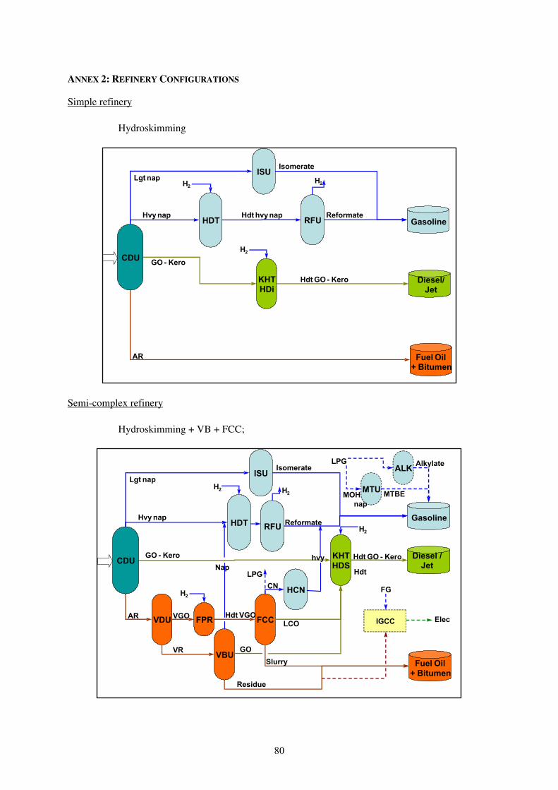
80

ANNEX 2: REFINERY CONFIGURATIONS

Simple refinery

Hydroskimming

Semi-complex refinery

Hydroskimming + VB + FCC;

CDU

KHTHDi

RFU Gasoline

Diesel/ Jet

Fuel Oil + Bitumen

ISU

HDT

GO - Kero

AR

Hvy nap

Lgt nap H 2 H2

H2

Isomerate

Reformate

Hdt GO - Kero

Hdt hvy nap

CDU KHTHDS

RFUGasoline

Diesel / Jet

Fuel Oil + Bitumen

ISU

HDT

VBU

VDU FPR FCC

HCN

MTU

ALK

GO - Kero

Lgt nap

Hvy napH2

H 2

H 2 H2

Isomerate

Reformate

Hdt

hvy

nap

Hdt GO - Kero

LPG

LPG

MOH MTBE

Alkylate

AR VGO

VR

Hdt VGO

Nap

LCO

CN

GO

Residue

Slurry

IGCC Elec

FG

81

Pre-treatment of FCC is optional. It aims to reduce the metal and the sulphur contained in the heavy gas oil before it enters the FCC; nevertheless, this unit consumes hydrogen. The use of a pre-treatment unit is essentially for diesel specifications. To meet gasoline specifications, post hydrotreatment of FCC output is the rule.

Hydroskimming + FCC + Delayed Coker

Coking is by far the most widely practiced means of reducing the carbon-hydrogen ratio of residual oils (Maples, 1993). From a chemical reaction viewpoint, coking can be considered as a severe thermal cracking process in which one of the end products is carbon (i.e., coke). Coking units convert heavy feedstocks into a solid coke and lower boiling hydrocarbon products which are suitable as feedstocks to other refinery units for conversion into higher value transportation fuels. Coking was primarily used to pretreat vacuum residuals to prepare coker gas oil streams suitable for feed to a catalytic cracker (Gary and Handwerk, 1994). This reduced the net refinery yield of low-priced residual fuel.

European and U.S. regulators continue to push for lower emitting gasoline and gasoil. Specifically, the sulphur content must be reduced significantly to achieve the required efficiency and emissions. Nearly all the sulphur (85 to 99%) in the typical refinery gasoline poll comes from FCC gasoline with a small amount coming from light straight run (CDTECH60). As a result, FCC gasoline is the place to focus in sulphur reduction. Typical FCC gasoline sulphur ranges from 1000 to 2000 ppm. This can be reduced considerably by hydrotreating the FCC feed although this is a capital cost intensive solution. In addition, FCC feed hydrodesulphurisation (HDS) by itself will likely not be sufficient when specifications for very low sulphur gasoline become effective. It will still be necessary to desulphurise the FCC gasoline to achieve the <30 ppm pool specification.

Hydroskimming + VB + HCU;

CDU KHTHDS

RFUGasoline

Diesel/Jet

Fuel Oil + Bitumen

ISU

HDT

CKU

VDU FPR FCC

HCN

MTU

ALK

GO - Kero

Lgt nap

Hvy napH2

H 2

H 2 H2

Isomerate

Reformate

Hdt

nap

Hdt GO - Kero

LPG

LPG

MOH MTBE

Alkylate

AR VGO

VR

Hdt VGO

Nap

LCO

CN

GO

COKE

Slurry

HCGO

82

In semi-complex refineries, the hydrodesulphurisation of residues is not common. The latter are a characteristic of more complex refineries.

Hydroskimming + HCU + Delayed Coker

Complete Conversion 60 http://www.cdtech.com/index.htm

CDU KHTHDS

RFUGasoline

Diesel/Jet

Fuel Oil + Bitumen

ISU

HDT

VBU

VDU HCU

GO - Kero

Lgt nap

Hvy nap H2

H 2 H2

Isomerate

Reformate

Hdt GO - Kero

AR VGO

VR

Nap

GO - Kero

GOResidue

H2

SRF Gas

MTU

ALK LPG

MOH MTBE

Alkylate

CDU KHTHDS

RFUGasoline

Diesel/Jet

Fuel Oil + Bitumen

ISU

HDT

CKU

VDU HCU

GO - Kero

Lgt nap

Hvy napH2

H 2 H2

Isomerate

Reformate

Hdt GO - Kero

AR VGO

VR

Nap

GO - Kero

GO

HCGO

Residue

H2

SRF Gas

MTU

ALK LPG

MOH MTBE

Alkylate

83

Hydroskimming + VB + FCC +HCU; a complex refinery that can even become a deep complex refinery depending on the number of conversion units that are added.

In this type of refinery configuration, “competition” exists for the use of vacuum gasoil (VGO) between the fluid catalytic cracker and the hydrocracker. Which process unit will convert the largest quantity will depend on the market demand for diesel, gasoline, and petrochemical feed.

The residue hydrocracker increases the proportion of hydrogen in heavy molecules – creating lighter products.

CDU KHTHDS

RFUGasoline

Diesel/Jet

Fuel Oil + Bitumen

ISU

HDT

VBU

VDU FCC

HCN

MTU

ALK

GO - Kero

Lgt nap

Hvy napH2

H 2

H 2 H2

Isomerate

ReformateHdt

hvy

nap

Hdt GO - Kero

LPG

LPG

MOH MTBE

Alkylate

AR VGO

VR

Nap

LCO

CN

GO

Residue

Slurry

HCU

Nap

GO KeroGOKero

SRF Gas

IGCC Elec

FG

84

ANNEX 3: AN INTRODUCTION TO THE REFINERY SECTOR

The product mix of refineries is changing towards more light products with a higher H/C ratio, as demand growth is concentrated in transportation markets. The refineries can respond to the hydrogen deficiency by adding hydrogen (a process called hydrocracking) or by removing carbon (a process called coking). This trend is apparent of regional refinery structures are compared. The higher the transportation fuel demand as a share of total fuel demand, the higher the coking and hydrocracking capacity.

The refinery market: inputs and basic downstream products

Crude oil varies in its weight and chemical form. The terms heavy and light are often used to refer to density. Heavy oil – more dense – is generally considered to be lower quality as it contains a higher share of heavy hydrocarbons. This means that distillation produces a larger yield of lower value oil products, such as heavy gas and fuel oil. Light oil is generally more desired as its distillation produces a lighter and, therefore, more profitable refined product slate.

Crude can also be termed as sweet and sour. This refers to the sulphur content of the crude. A high sulphur content – sour crude – is undesirable – for both processing and product quality, especially with the move to lower sulphur fuels under the European AutoOils programme – see Section 0. Equipment exists to process the sulphur out of the crude (e.g., desulphurisation units). Refiners will make an individual assessment of the value of investing in such equipment versus their outlook for the price differentials between different crude types. Ordinarily, it is found that the heavier the crude, the higher the quantities of sulphur, carbon and heavy metals, and the lower its hydrogen content (BREF, 2003).

Generally, any crude can be processed into any reasonable selection of products by a suitable choice of refining unit operations. Table 30 provides examples of process units which can be found in a refinery. Depending on each refinery, many different combinations of process units can be found. The cost of production will depend on the refining units required, which in turn depend on the crude selected (BREF, 2003). In theory, the production costs can be minimised by careful selection of the crude. In practice, however, refinery designs are often compromised by factors such as: the availability, the price and the composition of crude and changing market demands for product slate and specifications.

As in many industries, in the refining sector, capacity is an important factor in the overall industry economics – through economies of scale. However, in the refinery industry, the level of complexity or the level of conversion of crude oil into lighter and more valuable components that can be achieved is also important (PDC, 2004). 61

A refinery has to supply a certain area with a given demand for products. So with a given hardware, the crude is selected in order to supply properly the market for products. This requires using the flexibility of the hardware (this flexibility is limited though) and sometimes importing or exporting products in order to balance properly the refinery’s own production. Relative prices of crude, feedstock and products play a major role in the optimization of the refinery mode of operation (Becard, 2005). 61 PDC, 2004, “Study Contract for Investigation of EU Refineries’ Compliance with the Directive on Combating of Air Pollution for Industrial Plants”, EU Commission – DG Environment, December.

85

Table 30: Examples of process units in a refinery

GENERAL TYPE EXAMPLES

Separation Crude Distillation

Extraction

Reducing average molecular weight Visbreaking

Delayed coking

Fluid Catalytic Cracking

Heavy Oil Cracking

Hydrocracking

Quality Improvement Hydrotreating

Catalytic reforming

Isomerization

Increasing average molecular weight Alkylation

Source: Maples, 1993.

An oil refinery combines all process units to a lesser or greater degree. The complexity of the individual units, the combinations and the catalysts used are rarely fully disclosed (Deutsche Bank, 2002). In the highly competitive, generally low margin, world of global refining, the precise refinery yield – or refinery product output is a closely guarded competitive secret. As illustrated in Figure 18, oil refineries generate several products, either for final use or as intermediate feedstock. A proportion of the product streams is also used internally in the refinery for process fuel.

Figure 18: The oil refinery process and output

Crude Oil AtmosphericDistillation

LPG

Naphtha

Gasoline

Kerosene

Gasoil/Diesel

Heavy Fuel Oil

Other (Residuals/Lubricants)

Light

The “bottom of the barrel” has become more of a problem for refiners because heavier crude are being processed and the market for heavy residual fuel oils has been decreasing (Gary and Handwerk, 1994). Historically, the heavy residual fuel oils has been burned to produce electric power and to supply the energy needs of heavy industry, but more severe environmental fuel oils have caused many

86

of these users to switch to natural gas. Thus when more heavy residuals are in the crude there is more difficulty in economically disposing of them.

Process units and refinery types

In almost all cases, the crude oil is first processed in an atmospheric distillation unit. This separates out the major components in crude oil, based on boiling ranges. However, the use of only an atmospheric distillation – a topping refinery or a hydroskimming refinery– means that a large volume of the heavy residual oil product called fuel oil is produced. As the latter still contains a high proportion of more valuable distillate, most refineries now process this stream further using vacuum distillation.

The vacuum distillation unit (VDU) enables vacuum gas oil (VGO) to be recovered. This is often then sent for further processing in conversion plants into higher value components of end-products such as gasoline, diesel and heating oil (PDC, 2004). In many refineries, the VGO is processed in fluidised catalytic cracking units (FCCUs). There are alternative conversion plants in European refineries such as hydrocracking units (HCUs), although these are not common – see Table 2 for additional details.

In processing certain oils, lowering the carbon/hydrogen (C/H) ratio is needed. There are two ways which have been developed to lower the average molecular weight of an oil and to lower its C/H as well (Maples, 1993). These are:

Removal of carbon by forming coke (high C/H) – such as fluid catalytic cracking. FCC converts vacuum gas oil to a gasoline blending component and light cycle oil with a low cetane number for blending the gasoil / diesel pool. The gas oils produced through this process are for diesel fuel blending components, because of their high sulphur content and particularly for their very low cetane numbers;

Direct addition of hydrogen (infinite H/C) – through hydrocracking. A dual-function catalyst is needed which performs both cracking and hydrogen reactions. The degree of cracking depends greatly on the feedstock and, in general, the heavier the feed, the more middle distillate is produced. The hydrogen requirement of these units is extremely high, so that in general, it is necessary to have a hydrogen production plant as part of the hydro-cracker complex. In most cases, the units are run to maximise middle distillate production. In these cases, the distillate yield can be as high as 60 to 70%, the other products being saturated LPG, naphtha, and kerosene. The distillate produced by these units is characterised by a very low sulphur content and overall high quality.

The first of the above processes is easy and relatively inexpensive and is exemplified by delayed coking, fluid coking, and the coke deposited on FCC and other catalysts (Maples, 1993). The second process – hydrocracking - is more difficult and is much more expensive. Catalytic hydrocracking offers flexibility (in product yields) not available in other processes, but often at a higher price than fluid or thermal cracking.

The increases in capacity of the various processes have been made to meet the demands of the marketplace. Thus, the refinery has grown from a single simple distillation unit to a complex which might contain as many as 10-15 types of process units. Energy requirements will generally increase from configuration complexity.

87

Hydrotreating is a general term applied to processes where a feedstock is enhanced in some manner by passing it over a catalyst in the presence of hydrogen. The objective has most often been to reduce the sulphur content of feed, but also nitrogen and aromatics. Feedstocks stocks require more hydrogen than do virgin stocks of the same boiling ranges. Hydrogen consumption in standard cubic feet per barrel (SCFB) ranges 10-50 SCFB for virgin naphtha up to 300 SCFB for heavy gas oil. To reduce nitrogen may require 600-1,100 SCFB.

During the later stages of the fuel cycle, each fuel must be treated separately due to different fuel characteristics. Hence, some other units can be found in refineries, including those related to the manufacturing of gasoline (e.g., isomerisation, alkylation or oxygenates).

88

ANNEX 4: NUMBER OF REFINERY CONFIGURATIONS BY EU-25 COUNTRY

Table 31: 2004 Refinery breakdown in Europe by technology

COUNTRY

REFINERIES IN

OPERATION (2004)

SIMPLE SIMPLE

&

VISBREAKER

CAT CRACKING

CAT CRACKING

& COKER

HYDRO CRACKING

HYDRO CRACKING & COKER

BOTH CC & HC

BOTH & COKER

Austria 1 0 0 1 0 0 0 0 0

Belgium 5 2 1 2 0 0 0 0 0

Cyprus 1 1 0 0 0 0 0 0 0

Czech Rep62 3 0 1 1 0 1 0 0 0

Denmark 2 1 1 0 0 0 0 0 0

Finland 2 0 0 1 0 0 0 1 0

France 13 163 0 11 0 0 0 1 0

Germany64 16 1 1 6 0 565 1 1 1

Greece 4 2 0 1 0 0 0 1 0

Hungary66 1 0 0 0 1 0 0 0 0

Ireland 1 1 0 0 0 0 0 0 0

Italy 17 3 4 3 1 3 0 3 0

Lithuania 1 0 0 1 0 0 0 0 0

Netherlands 6 1 1 1 0 1 1 1 0

Poland67 2 1 0 0 0 0 0 1 0

Portugal 2 1 0 0 0 0 0 1 0

Slovakia 1 0 0 0 0 0 0 1 0

Slovenia 1 1 0 0 0 0 0 0 0

Spain 9 1 1 2 1 1 0 2 1

Sweden 5 4 0 0 0 0 0 1 0

UK, England 11

3 0 6 1 1 0 0 0

Total 104 24 10 36 4 12 2 14 2

Source: adapted from Oil & Gas Journal (2004), Concawe.

Refineries are to be found in every Western European state other than Luxemburg and there are areas in Europe where are multiple refineries at the same location (e.g., Rotterdam and Antwerp). The processes that operate at the various refineries vary quite significantly although most in Europe have common process units and common operational practices. In 2004, EU 25 had a total crude distillation capacity close to 15 million barrels per day (mbd). 68 In the same year, the US’s production capacity reached over 16mbd. However, the US consumed close to 20.8mbd. Unlike the European counties, the United States have a gasoline deficit and gas oil surplus.

62 One refinery is not in operation in 2004. 63 Lubes manufacturing 64 One refinery was not in operation in 2004. 65 One hydrocracking refinery is dedicated to lube oil manufacturing 66 One refinery was not in operation in 2004. 67 Three refineries were not in operation in 2004. 68 Central EU average: (A, Cz, H, Pd, Slovakia., Slovenia); Mediterranean average (Gc, It, Pg, Sp, Tk); NE Europe average (B, F, G, Ir, Nt, UK); Scandinavian average (Dk, Fi, Ny, Sw).

89

ANNEX 5: REFINERY CAPACITY UTILISATION RATE IN OECD COUNTRIES

CAPACITY UTILISATION AVERAGE 2004-MAY 2005

US(50) 89.1

CANADA 90.9

MEXICO 76.1

AUSTRIA 86.9

BELGIUM 84.2

CZECH REPUBLIC 62.9

DENMARK 90.4

FINLAND 97.6

FRANCE 87.1

GERMANY 95.4

GREECE 91.2

HUNGARY 76.7

IRELAND 91.7

ITALY 75.8

NETHERLAND 81.2

NORWAY 83.5

POLAND 92.8

PORTUGAL 78.9

SPAIN 87.1

SWEDEN 90.0

SWITZERLAND 75.5

TURKEY 73.4

UK 90.5

JAPAN 81.8

KOREA 85.4

AUSTRALIA 83.0

NEW ZEALAND 95.3

OECD North America 88.3

OECD Europe 85.7

OECD Pacific 83.2

OECD 86.4

Other Europe 84.1

Other Asia 84.4

Average EU-15: over 87%.

90

ANNEX 6: CRUDE INPUT FOR EACH REFINERY CONFIGURATION, ACCORDING TO REGION

NWE 1-HSK 2- + VB +

FCC 4- + VB + HCU

5- + DC + HCU

6- + FCC +

HCU + VB

TOTAL NWE

Config., vol% 10% 55% 11% 5% 15% 100% 1-Mix Arab.-Iran. 5% 9% 9% 16% 17% 10% 2-BFO or North Sea sweet 60% 49% 49% 45% 41% 48% 3-Bonny light or sweet light West African 15% 14% 14% 11% 9% 13% 4-Urals 9% 23% 22% 22% 31% 22% 5-Sahara blend 11% 6% 7% 6% 2% 6%

Total NWE 100% 100% 100% 100% 100% 100% Total kbbl 200 779 1 123 196 231 235 105 792 313 099 2 056 514 API 37.3 36.1 36.2 35.7 35.0 36.0 Specific Gravity 0.84 0.84 0.84 0.85 0.85 0.84 S wt% 0.44 0.65 0.64 0.77 0.88 0.67

CENTRAL 1-HSK 2- + VB + FCC

4- + VB + HCU

5- + DC + HCU

6- + FCC + HCU +

VB

TOTAL CENTRAL

Config., vol% 6% 42% 7% 0% 39% 100% 1-Mix Arab.-Iran. 5% 10% 10% - 15% 12% 2-BFO or North Sea sweet 5% 8% 8% - 5% 6% 3-Bonny light or sweet light West African 0% 0% 0% - 0% 0% 4-Urals 79% 80% 80% - 80% 80% 5-Sahara blend 11% 3% 3% - 0% 2%

Total Central 100% 100% 100% - 100% 100% Total kbbl 26 220 182 717 32 047 - 170 418 437 057 API 33.9 33.2 33.2 - 32.7 33.0 Specific Gravity 0.86 0.86 0.86 - 0.86 0.86 S wt% 1.12 1.22 1.22 - 1.31 1.26

MED 1-HSK 2- + VB

+ FCC 4- + VB

+ HCU 5- + DC

+ HCU

6- +

FCC + HCU +

VB

TOTAL MED

Config., vol% 13% 44% 4% 1% 32% 100% 1-Mix Arab.-Iran. 20% 36% 36% 44% 46% 38% 2-BFO or North Sea sweet 15% 15% 15% 10% 10% 13% 3-Bonny light or sweet light West African 9% 7% 7% 7% 6% 7% 4-Urals 20% 25% 25% 26% 26% 25% 5-Sahara blend 36% 17% 17% 13% 12% 18% Total Med 100% 100% 100% 100% 100% 100% Total kbbl 234 204 782 690 72 835 21 615 564 670 1 760 737 API 37.2 35.0 35.0 34.3 34.1 35.0 Specific Gravity 0.84 0.85 0.85 0.85 0.85 0.85 S wt% 0.76 1.10 1.10 1.25 1.29 1.13

91

ANNEX 7: CALCULATED REFINERY PRODUCTION

NORTH WEST EUROPE (KT) 1-

HSK 2- +VB+FCC 4- +VB+HCU 5- +DC+HCU 6-

+VB+FCC+HCU

Number of Refineries 12 21 5 3 5 Output 26024 139974 29985 14393 40812 LPG 372 3207 752 429 1450 Propane 202 3158 281 161 615 Butane 170 49 471 268 834 Naphtha 3771 11757 1520 919 3861 Gasoline 3548 45310 8028 3864 11268 Eurosuper 95 3316 24917 5100 2375 7190 Premium 98 232 1434 298 137 414 Export (US / 92) 0 18959 2630 1352 3664 Jet A1 1632 10099 2099 963 2914 AGO 6149 38057 11100 5925 13560 IGO 2298 12855 930 720 2458 HFO 7744 15187 4828 871 4218 LS HFO 7744 0 4828 871 0 HS HFO 0 0 0 0 4218 LS Bunker 0 15187 0 0 0 HS Bunker 0 0 0 0 0 Bitumen 488 2989 620 0 864 Sulfur 22 513 108 84 220 Coke 0 0 0 617 0 Fuel and loss 1845 17424 3406 1649 5147

MEDITERRANEAN EUROPE (KT)

1-HSK

2- +VB+FCC 4- +VB+HCU 5- +DC+HCU 6-

+VB+FCC+HCU

Number of Refineries 12 18 2 1 10

Output 30238 101029 9534 2984 74133 LPG 346 3185 222 82 1913 Propane 246 1848 93 31 1041 Butane 100 1337 129 50 872 Naphtha 2483 7524 378 492 11451 Gasoline 5674 30764 2519 495 16241 Eurosuper 95 4260 15910 1496 469 11786 Premium 98 246 916 86 26 678 Export (US / 92) 1168 13938 938 0 3777 Jet A1 1591 5915 556 166 4381 AGO 7000 28000 2882 859 22712 IGO 2103 7463 1312 519 6840 HFO 10037 14105 877 175 7256 LS HFO 2308 0 877 175 0 HS HFO 40 14105 0 0 0 LS Bunker 7688 0 0 0 0 HS Bunker 0 0 0 0 7256 Bitumen 961 3477 724 0 2760 Sulfur 45 598 63 27 579 Coke 0 0 0 169 0

Fuel and loss 2282 12104 1112 332 9028

92

CENTRAL EUROPE (KT) 1-

HSK 2- +VB+FCC 4- +VB+HCU 5- +DC+HCU 6-

+VB+FCC+HCU

Number of Refineries 1 4 1 3

Output 3470 24269 4328 0 22544 LPG 42 857 111 0 486 Propane 20 410 38 0 255 Butane 22 448 72 0 231 Naphtha 0 2214 164 0 1639 Gasoline 705 6423 1107 0 5740 Eurosuper 95 300 4395 779 0 4194 Premium 98 0 253 45 0 241 Export (US / 92) 405 1775 284 0 1304 Jet A1 129 994 176 0 949 AGO 440 6870 1298 0 6990 IGO 615 1421 676 0 1782 HFO 1532 4315 478 0 3940 LS HFO 0 0 0 0 0 HS HFO 1532 4315 0 0 3940 LS Bunker 0 0 478 0 0 HS Bunker 0 0 0 0 0 Bitumen 0 1013 282 0 843 Sulfur 7 163 35 0 174 Coke 0 0 0 0 0 Fuel and loss 281 2783 547 0 2856

NWE CEN MED

6- +VB+FCC+HCU+IGCC

6- +VB+FCC+HCU+IGCC

6- +VB+FCC+HCU+IGCC

Number of Refineries 5 3 10

Output 37497 19853 68808 LPG 1450 487 1913 Propane 616 255 1041 Butane 834 231 871 Naphtha 3861 1640 11451 Gasoline 11271 5744 16260 Eurosuper 95 7190 4194 11786 Premium 98 414 241 678 Export (US / 92) 3667 1309 3796 Jet A1 2914 949 4381 AGO 11300 6990 24600 IGO 5498 2909 6599 HFO 0 0 0 LS Bunker 0 0 0 HS Bunker 0 0 0 Bitumen 864 843 2760 Sulfur 339 292 844 Coke 0 0 0 Fuel and loss 6339 4269 9499

93

ANNEX 8: REFINERY PROCESS FUELS COMPOSITION BY REGION AND CONFIGURATION

Refinery fuel gas (RFG)

The majority of the fuel used in a refinery is gas (methane, ethane, etc.) which is internally generated in the different refinery processes and collected in the refinery gas system, but has to consumed quickly and cannot normally be sold as a valuable product. On some occasion there are buyers of it like petrochemical plants that are situated next to a refinery. RFG, if properly treated, is a low polluting fuel. Most of the refinery fuel gas systems have two or three alternative sources of supply: refinery gas, imported gas and liquefied petroleum gas. Normally, most or all of the gaseous and liquid refinery fuels are by-products of refinery process. Nevertheless, in some cases, fuel (whether its oil or gas) cannot be consider as a by-product.

Liquid refinery fuel (heavy fuel oil - HFO)

Heavy fuel oil – HFO - used in the refinery is normally a mixture of the residues from atmospheric and/or vacuum distillation and conversion and cracking processes. Liquid refinery fuels are normally used for process start-ups (BREF, 2003).

Solid fuels

Petroleum coke that is generated and subsequently burned in the fluid catalytic process can be assimilated to a solid fuel. It can also be gasified as a refinery fuel gas source. Coal as imported fuel is not applied in European refineries

NWE Fuel GJ 1-

HSK 2-

+VB+FCC 4-

+VB+HCU 5-

+DC+HCU

6- +VB+FCC

+HCU

Crude kt 26 762 150 809 31 027 14 232 42 298 Crude wt% 10% 55% 11% 5% 15% GJ Fuel to electricity generation 56 382 509 741 99 661 49 351 141 758 Fuel to steam generation 8 546 82 449 19 135 8 533 22 380 Fuel to process units 20 086 229 911 31 433 16 889 58 087 Total fuel consumed 85 013 822 101 150 229 74 774 222 226 % Fuel to electricity generation 66% 62% 66% 66% 64% Fuel to steam generation 10% 10% 13% 11% 10% Fuel to process units 24% 28% 21% 23% 26% Total fuel consumed 100% 100% 100% 100% 100%

94

MED Fuel GJ 1-HSK

2- +VB+FCC

4- +VB+HCU

5- +DC+HCU

6- +VB+FCC

+HCU

Crude kt 31 233 105 740 9 840 2 934 76 698 Crude wt% 13% 44% 4% 1% 32% GJ Fuel to electricity generation 74 186 360 972 32 754 9 070 246 539 Fuel to steam generation 13 778 56 705 5 799 1 309 35 416 Fuel to process units 23 986 162 009 10 990 3 370 108 396 Total fuel consumed 111 949 579 686 49 543 13 749 390 351 % Fuel to electricity generation 66% 62% 66% 66% 63% Fuel to steam generation 12% 10% 12% 10% 9% Fuel to process units 21% 28% 22% 25% 28% Total fuel consumed 100% 100% 100% 100% 100%

Central

CEN Fuel GJ 1-HSK Med

2- +VB+FCC

Med

4- +VB+HCU

Med

6HSK +VB+FCC

+HCU Med

Crude kt 3 567 24 966 4 379 23 354 Crude wt% 4% 26% 5% 24% GJ Fuel to electricity generation 9 355 81 341 15 431 79 445 Fuel to steam generation 1 789 11 308 2 542 12 883 Fuel to process units 2 894 38 950 5 372 31 536 Total fuel consumed 14 038 131 599 23 345 123 864 % Fuel to electricity generation 67% 62% 66% 64% Fuel to steam generation 13% 9% 11% 10% Fuel to process units 21% 30% 23% 25% Total fuel consumed 100% 100% 100% 100%

95

ANNEX 9: CRUDE OIL AND REFINERY FEEDSTOCK PRICES

Table 32: Crude oil and refinery feedstock prices

FEEDSTOCK &

PRODUCTS, USD/BARREL USD/TONNE

CRUDE OILS

Iranian Light 279

Iranian Heavy 263

Arabian Light 267

Arabian Heavy 231

Brent 318

Forties 325

Oseberg 312

Bonny Light 311

Urals 266

Saharan Blend 327

OTHER FEEDSTOCKS PRICE BASIS

Methanol CIF 256

MTBE CIF 559

Natural Gas CIF 21669

69 For natural gas, 2004 Europe CIF prices are taken. This value equals to a natural gas price of 4.56$/MMBtu.

96

Table 33: Prices based on Platts year 2004

FEEDSTOCK &

PRODUCTS, USD/TON PRICE BASIS NWE MED

LPG

Propane CIF 390 387

Butane CIF 368 360

Gasoline

Naphtha FOB 397 352

Eurosuper 95 FOB 415 416

Premium 98 FOB 426 427

Export (US / 92) FOB 389 391

Middle Distillates

Jet A1 CIF 399 406

AGO CIF 455 462

IGO CIF 357 366

Fuel Oil

LS HFO FOB 159 169

HS HFO FOB 142 155

LS Bunker FOB 143 151

HS Bunker FOB 129 139

Others

Bitumen 200 200

Sulphur FOB 65 65

Coke 50 50

Fuel and loss FOB 159 159

97

ANNEX 10: PRODUCT SPECIFICATIONS

Between Europe and the Rest of the World (RW), trade of gasoil products can only take place if the sulphur levels of fuels comply with EU regulation. Table 34 provides the evolution of the main specifications in Europe.

Table 34: Euro 2, 3 and 4 specifications

Source: http://www.un.org/esa/gite/cleanfuels/ee.pdf

Currently, the specifications for petrol and diesel sold in the European Union are laid down in Directive 2003/17/EC amending Directive 98/70/EC on the quality of petrol and diesel fuels. 70 The primary objective of the latest directive is to implement the staged introduction of sulphur-free road fuels, starting in 2005 and, subject to review by the Commission in the case of diesel fuel, requiring 100% provision by 2009. Table 35 summarises the specification timetable for the introduction of sulphur-free road fuels to the European market.

70 The sulphur (SO2) content of heavy fuels used in large ships is also to be reduced to 1.5% by 2007 after Parliament agreed to a compromise with Council on the marine fuels directive. This figure is to be brought down to 0.5% in port areas where ships will be required to switch off their engines and use shore-side electricity.

98

Table 35: Quality of gasoline and diesel in Europe

GASOLINE 1998 JAN 00 JAN 03 JAN 05 JAN 08

Sulphur (max.) 500 ppm 150 ppm - 50 ppm* 10 ppm

Benzene (%vol.) 5% max. 1% max. - 1% max. **

Aromatics (%vol.)

- 42% max. - 35% max. **

Olefins (%vol.) - 18% max. - 18% max. **

Oxygen (%m) 2.5-3.7 max 2.7 max. - - -

DIESEL FUEL 1998 JAN 00 JAN 03 JAN 05 JAN 08

Sulphur (max.) 500 ppm 350 ppm - 50 ppm* 10 ppm

Cetane (min.) 49 51 - 51 **

Polyaromatics - 11% max. - 11% max. **

Specific gravity (max.)

860 845 - 845 **

Source: IFP (2004)

.

* Motor fuels meeting the 10ppm sulphur limit must be available on the market ** The Commission may set new values before 2006.

Directive 2003/17/EC also introduces limits on the level of sulphur in fuel provided for use by agricultural tractors and non-road mobile machinery into Directive 98/70/EC. There are currently no specific requirements controlling the fuel quality used by this class of vehicle and the directive limits the sulphur in fuels for these vehicles to 2000 mg/kg reducing to 1000 mg/kg in 2008. This is already achieved in practice by the Sulphur Content of Liquid Fuels Directive, which applies identical requirements to gasoil used in such appliances as boilers. Similarly, heavy fuel oil sulphur content will be limited to 1% from 1 January 2003 as compared to a current specification of 3.5%, with the option of having a limit on total sulphur dioxide emissions rather than fuel sulphur. This is important to oil refineries which burn sulphur free gas as well as fuel oil.

99

Table 36: Quality of heating oil and fuel oil in Europe

HEATING OIL 1998 JAN 00 JAN 03 JAN 05 JAN 08

Sulphur (max.) 0.2% - - - 0.1%

FUEL OIL 1998 JAN 00 JAN 03 JAN 05 JAN 08

Sulphur (max.)

- - 1% - -

Source: IFP (2004).

The Sulphur Content of Liquid Fuels Directive (1999/32/EC) also limits the sulphur content of gas oil, including that for marine use to 0.2% from 1st July 2000 (no change apart from marine) and to 0.1% from 1st January 2008. As part of its ship emissions strategy, the European Commission presented in November 2002 a proposal to reduce the sulphur content of marine fuels. The main provisions finalised and approved in 2005 include a 0.1% sulphur limit on fuel used by inland vessels and by seagoing ships at berth in EU ports, from 1st January 2010. They also implement a 1.5% sulphur limit for marine fuels sold in the Union.

Source: http://www.un.org/esa/gite/cleanfuels/ee.pdf

100

Table 37: Product specifications

Jet Euro V (IV)Soufre, wt% < 0.3Densité 0.775 < < 0.840Acidité, mgKOH/g < 0.015Aromatiques, vol% < 20Oléfines, vol% < 5.0Mercaptans, wt% < 0.0020Temp 10 vol% distillé, °C < 204PCI, MJ/kg > 42.8Viscosité à 20°C, cSt < 8.0Point de fumée, mm > 25Point final, °C < 300Point de congélation, °C < -47Point d'éclair, °C > 38

Diesel Euro IV Euro VSoufre, wt% < 0.005 < 0.001Densité 0.820 < < 0.845Cetane mesuré > 51Cetane index > 46Temp 95 vol% distillé, °C < 360Point d'éclair, °C > 55Point de trouble, °C (Eté) < +5Point de trouble, °C (Hiver) < -5TLF, °C (Eté) < 0TLF, °C (Hiver) < -15Evaporation à 250°C, vol% < 65Evaporation à 350°C, vol% > 85Polyaros, wt% < 11Esters, vol% < 5Viscosité à 40°C, cSt 2.00 < < 4.50

US Regular 9.0# 2010Road Octane (RON+MON)/2 > 87RVP, bar < 0.62 (9.0 psi)Soufre, wt% < 0.001Densité 0.720 < < 0.775Aromatiques, vol% < 35Benzène, vol% < 1Oléfines, vol% < 20Oxygène, wt% < 2.0Evaporation à 100°C, vol% 46 < < 71

Export & Reg 92 2010RON > 92RVP, kPa (Eté) < 65RVP, kPa (Hiver) < 80Soufre, %pds < 0.15Densité 0.710 < < 0.765Aromatiques, %vol -Benzène, %vol -Oléfines, %vol -Point final, °C < 205

Euro Super 95 (& East) Euro IV Euro VRON > 95MON > 85RVP, bar (Eté) 0.45 < < 0.60RVP, bar (Hiver) 0.60 < < 0.90Soufre, wt% < 0.005 < 0.001Densité 0.720 < < 0.775Aromatiques, vol% < 35Benzène, vol% < 1Oléfines, vol% < 18Mercaptans, wt ppm < 15Oxygène, wt% < 2.7Methanol, vol% < 3.0Ethanol, vol% < 5.0Ethers, vol% < 15.0Evaporation à 70°C, vol% (Eté) 20.0 < < 48.0Evaporation à 70°C, vol% (Hiver) 22.0 < < 50.0Evaporation à 100°C, vol% 46 < < 71Evaporation à 150°C, vol% > 75Point final, °C < 210

Prem 98 Euro IV Euro VRON > 98MON > 87RVP, bar (Eté) 0.45 < < 0.60RVP, bar (Hiver) 0.60 < < 0.90Soufre, wt% < 0.005 < 0.001Densité 0.720 < < 0.775Aromatiques, vol% < 35Benzène, vol% < 1Oléfines, vol% < 18Mercaptans, wt ppm < 15Oxygène, wt% < 2.7Methanol, vol% < 3.0Ethanol, vol% < 5.0Ethers, vol% < 15.0Evaporation à 70°C, vol% (Eté) 20.0 < < 48.0Evaporation à 70°C, vol% (Hiver) 22.0 < < 50.0Evaporation à 100°C, vol% 46 < < 71Evaporation à 150°C, vol% > 75Point final, °C < 210

101

IGO Euro V (IV)Soufre, wt% < 0.2 ?Densité 0.830 < < 0.880Evaporation à 250°C, vol% < 65Evaporation à 350°C, vol% > 85Cetane index > 40Point d'éclair, °C > 55Point de trouble, °C < 2Point d'écoulement, °C < -9Viscosité à 20°C, cSt 3 < < 7.5

LS HFO Euro V (IV)Soufre, wt% < 1Point d'éclair, °C > 70Evaporation à 250°C, vol% < 65Evaporation à 350°C, vol% < 85Viscosité à 20°C, cSt > 9.5Viscosité à 100°C, cSt < 40

HS HFO Euro V (IV)Soufre, wt% < 2.5Point d'éclair, °C > 70Evaporation à 250°C, vol% < 65Evaporation à 350°C, vol% < 85Viscosité à 20°C, cSt > 9.5Viscosité à 100°C, cSt < 40

LS Bunker Euro IV Euro VSoufre, wt% < 4.5 < 0.7 ?Densité < 0.991Point d'éclair, °C > 60Point d'écoulement, °C < 30Viscosité à 100°C, cSt < 25 / 35Viscosité à 50°C, cSt < 180 / 380

HS Bunker Euro IV Euro VSoufre, wt% < 4.5 < 2.0 ?Densité < 0.991Point d'éclair, °C > 60Point d'écoulement, °C < 30Viscosité à 100°C, cSt < 25 / 35Viscosité à 50°C, cSt < 180 / 380

Bitumen 20 / 30 35 / 50 50 / 70 70 / 100 160 / 120Pénétrabilité @25°C, x 0.1 mm 20 < < 30 35 < < 50 50 < < 70 70 < < 100 160 < < 220TBA, °C 55 < < 63 50 < < 58 46 < < 54 43 < < 51 35 < < 43Point d'éclair, °C > 240 > 240 > 230 > 230 > 220Paraffines, wt% < 4.5 < 4.5 < 4.5 < 4.5 < 4.5

102

ANNEX 11: RUNNING EXPENSES AND INVESTMENT COSTS PER AREA AND CONFIGURATION

NWE 1-

HSK 2- + VB

+ FCC

4- + VB +

HCU 5- + DC

+ HCU

6- + FCC

+ HCU +

VB

Estimated Unit Investment / raff MMUSD 258 1332 950 1289 1635 Variable Costs USD / t 0.11 0.70 0.18 0.38 0.65 Catalysts & Chemicals USD / t 0.11 0.70 0.18 0.38 0.65

Fixed Costs USD / t 9.24 14.83 12.25 21.74 15.46 Personnel USD / t 1.16 1.85 1.53 2.72 1.93

Maintenance USD / t 4.62 7.42 6.12 10.87 7.73

Overheads USD / t 2.31 3.71 3.06 5.44 3.86

Insurance USD / t 1.16 1.85 1.53 2.72 1.93

Working Capital USD / t 0.00 0.00 0.00 0.00 0.00

Running Expenses USD / t 9.35 15.54 12.43 22.13 16.11

MED 1-

HSK 2- + VB

+ FCC

4- + VB +

HCU 5- + DC

+ HCU

6- + FCC

+ HCU +

VB

Estimated Unit Investment / raff MMUSD 316 1120 959 961 1573

Variable Costs USD / t 0.16 0.80 0.29 0.59 0.74

Catalysts & Chemicals USD / t 0.16 0.80 0.29 0.59 0.74

Fixed Costs USD / t 9.71 15.25 15.59 26.19 16.41

Personnel USD / t 1.21 1.91 1.95 3.27 2.05

Maintenance USD / t 4.85 7.62 7.80 13.10 8.20

Overheads USD / t 2.43 3.81 3.90 6.55 4.10

Insurance USD / t 1.21 1.91 1.95 3.27 2.05

Working Capital USD / t 0.00 0.00 0.00 0.00 0.00

Running Expenses USD / t 9.87 16.04 15.89 26.78 17.15

CEN

NWE

PRICES 1-

HSK 2- + VB

+ FCC

4- + VB +

HCU 5- + DC

+ HCU

6- + FCC

+ HCU +

VB

Estimated Unit Investment / raff MMUSD 377 1124 884 1786

Variable Costs USD / t 0.17 0.85 0.30 0.87

Catalysts & Chemicals USD / t 0.17 0.85 0.30 0.87

Fixed Costs USD / t 8.47 14.41 16.15 18.35

Personnel USD / t 1.06 1.80 2.02 2.29

Maintenance USD / t 4.23 7.21 8.08 9.17

Overheads USD / t 2.12 3.60 4.04 4.59

Insurance USD / t 1.06 1.80 2.02 2.29

Working Capital USD / t 0.00 0.00 0.00 0.00

Running Expenses USD / t 8.64 15.27 16.46 19.22

CEN

MED

PRICES 1-

HSK

2-HSK

+ VB +

FCC

4-HSK +

VB +

HCU

5-HSK

+ DC +

HCU

6-HSK +

FCC +

HCU + VB

Estimated Unit Investment / raff MMUSD 377 1124 884 1786

Variable Costs USD / t 0.17 0.85 0.30 0.87

Catalysts & Chemicals USD / t 0.17 0.85 0.30 0.87

Running Expenses ** USD / t 8.64 15.27 16.46 19.22 ** These include fixed costs which are the same as in the NWE price configuration since investment costs are equal.

103

ANNEX 12: CRUDE OIL IN EUROPE

Figure 19: Crude oil imports in OECD Europe from OPEC

Algeria8% Indonesia

0%

Iran19%

Iraq4%

Kuwait3%

Libya24%

Nigeria11%

Neutral Zone0%

Qatar0%

Saudi Arabia29%

United Arab Emirates0%

Venezuela2%

Source: IEA.

Figure 20: Crude oil imports in OECD Europe from Former Soviet Union

Azerbaijan3% Kazakhstan

7%

Russia89%

Ukraine0%

Other Former USSR0%

Source: IEA.

104

BFO. Brent blend is a light and sweet, North Sea crude oil. 71Most of it is refined in Northwest Europe, but significant volumes move to the U.S. Gulf and East Coasts and to the Mediterranean.72 Brent is now quoted on the IPE forward market as an average Brent, Forties, Oseberg.

Urals. Russia is the most important exporter of crude oil to Europe. The main crude type it exports is Urals. In Europe, Urals imports can either be CIF (Cost, insurance, freight) Med– the port of discharge being Augusta in Sicily - or CIF Rotterdam. Norway is Europe’s second most important exporter of crude oil. 73 74

Mix of Arabian light, Arabian heavy, Iranian light and Iranian heavy (following the European import ratio)

Nigerian Bonny Light

Saharan Blend

71 Brent Blend is actually a combination of crude oil from 15 different oil fields in the Brent and Ninian systems located in the North Sea. Its API gravity is 38.3 degrees (making it a “light” crude oil, but not quite as “light” as WTI), while it contains about 0.37 percent of sulphur (making it a “sweet” crude oil, but again slightly less “sweet” than WTI). Brent blend is ideal for making gasoline and middle distillates, both of which are consumed in large quantities in Northwest Europe, where Brent blend crude oil is typically refined. However, if the arbitrage between Brent and other crude oils, including WTI, is favourable for export, Brent has been known to be refined in the United States (typically the East Coast or the Gulf Coast) or the Mediterranean region. 72 http://www.nymex.com/jsp/markets/bco_fut_descri.jsp 73 Prices for crude oil can either include freight costs – CIF - , or have them paid by the customer – FOB. CIF - Cost, insurance, freight – is a pricing term indicating that the cost of the goods, insurance, and freight are included in the quoted price. For FOB – Free on Board -, the price actually charged at the point of loading. 74 The main consumers of CIF Med are France, Italy and Spain.

105

ANNEX 13: MAIN COUNTRIES IMPORTING AND EXPORTING REFINED OIL PRODUCTS INTO AND FROM OECD EUROPE

LIQUEFIED PETROLEUM

GASES 2000 2001 2002 2003

IMPORTS

Algeria 5259 4665 4363 2650

Russia 580 742 459 790

EXPORTS from OECD Europe

Turkey 272 97 353 1044

United States 106 199 202 1075

NAPHTHA 2000 2001 2002 2003

IMPORTS

Algeria 2882 3192 3523 2475

Russia 694 796 1506 2472

Egypt 915 528 710 1130

Libya 1659 1965 1765 1740



MOTOR GASOLINE 2000 2001 2002 2003

IMPORTS

Norway 1371 974 1361 1945

Russia 327 269 289 765

Algeria 273 86 417 538

Egypt 63 140 565 562

106


United States 7483 9283 11908 12406

Libya 695 958 1088 1370

Nigeria 759 377 684 1111

Lebanon 436 630 638 723

KEROSENE TYPE JET FUEL 2000 2001 2002 2003

IMPORTS

Kuwait 1039 1565 1268 1907

United Arab Emirates 1016 2249 2051 1983

Algeria 638 451 663 485


Switzerland 994 990 795 653


GAS/DIESEL OIL 2000 2001 2002 2003

IMPORTS

Russia 8730 11760 14369 14481

Latvia 2254 2409 2692 2878

Norway 1722 1410 2401 2417

Algeria 1407 1748 1024 1102


Switzerland 3073 2835 3199 3032

United States 1694 894 1251 1566

Tunisia 779 951 604 915

107

FUEL OIL (RESIDUAL) 2000 2001 2002 2003

IMPORTS

Russia 5679 7424 8815 7515

Estonia 3264 3347 3925 2617

Libya 2549 1933 2257 2210

United States 690 1146 1172 223

Norway 423 588 1093 750

Algeria 130 80 445 677


United States 6458 7306 5869 6793

Norway 2441 2148 1679 1888

Singapore 1311 1859 2238 577

PETROLEUM COKE 2000 2001 2002 2003

IMPORTS

United States 6899 6312 5835 6524

Venezuela 938 1399 1481 1593


Norway 176 89 122 93

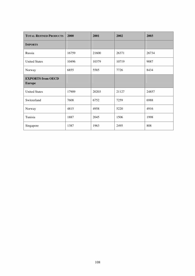
108

TOTAL REFINED PRODUCTS 2000 2001 2002 2003

IMPORTS

Russia 16759 21600 26371 26734

United States 10496 10379 10719 9087

Norway 6855 5585 7726 8434


United States 17909 20203 21127 24857

Switzerland 7608 6752 7259 6988

Norway 4815 4958 5220 4916

Tunisia 1887 2045 1506 1998

Singapore 1387 1963 2495 808

109

ANNEX 14: REFINERY PROJECTS AND ASSOCIATED COSTS

CAPACITY (MB/D) ADDITIONS INVESTMENT (BILLION DOLLARS) 2004 2010 2020 2030 2005-2010 2011-2020 2021-2030 2004-2030 OECD 44.3 45.9 49.6 51.8 13.6 29.8 18.1 61.4

OECD North America 20.5 22.1 24.6 25.6 13.3 21.4 9.1 43.9

OECD Pacific 8.1 8.1 8.9 9.7 0.3 5.0 4.9 10.1OECD Europe 15.7 15.7 16.1 16.6 0.0 3.3 4.1 7.4

TE 9.5 9.5 9.7 10.2 8.2 9.8 13.4 31.4 DEV 29.3 37.2 47.1 55.7 68.1 82.8 71.5 222.4China 6.1 8.8 12.5 14.6 17.6 25.5 14.0 57.0India 2.4 3.2 4.2 5.2 4.7 5.3 5.9 15.9Other DEV 12.0 14.4 17.1 19.9 21.0 25.4 24.9 71.2ME 7.0 8.8 10.7 12.9 20.8 20.5 21.1 62.4Iran 1.5 1.7 2.2 2.6 1.9 5.8 3.3 11.0Iraq 0.6 0.8 1.0 1.2 1.8 2.1 2.2 6.1Kuwait 0.9 1.3 1.4 1.4 5.0 0.6 0.6 6.1Qatar 0.1 0.2 0.3 0.3 0.6 0.6 0.6 1.8Saudi Arabia 2.1 2.6 3.4 4.5 7.2 8.2 10.8 26.2UAE 0.7 0.8 0.9 1.1 0.7 0.9 1.5 3.1Other ME 1.1 1.4 1.6 1.8 3.8 2.2 2.1 8.1NA 1.8 2.1 2.6 3.1 4.0 6.1 5.7 15.9Algeria 0.5 0.7 0.9 1.0 3.13 2.92 2.46 8.5Egypt 0.8 0.8 0.9 1.1 0.4 1.2 1.8 3.4Libya 0.4 0.4 0.6 0.7 0.5 1.5 1.1 3.1Other NA 0.2 0.2 0.2 0.3 0.0 0.5 0.4 0.9World 83.1 92.7 106.4 117.8 89.9 122.3 103.0 315.3

Source: WEO 2005 (forthcoming)

110

ANNEX 15: QUALITY OF THE HFO M-100 ASSUMMED IN THE CASE STUDY

M-100 TOTAL M-100 VAC. DISTILLATION

VGO VR

Yield wt% 100 37.7 62.3

Initial Boiling Point °C 450 450 550

Final Boiling Point °C - 550 -

Specific gravity 0.9530 0.9242 1.0151

Sulphur content wt% 2.58 1.96 2.96

Viscosity @ 80 °C cSt 82 16 4700

111

ANNEX 16: INVESTMENT IN RUSSIAN REFINERIES TO MEET EURO V SPECIFICATIONS

Table 38: Russian HSK capacities taken into account, and required capacities to meet Euro V specifications


UTILISATION RATE RUSSIAN HSK CURRENT

SPECIFICATIONS RUSSIA HSK EURO 100PPM



TYPE OF

PROCESS PROCESS KT/YR % KT/YR %

Crude Distillation

Atm. Distillation 49 117 100 49 117 100

Vacuum Distillation 11 364 100 11 364 100

Conversion Visbreaking 1 908 100 1908 100

Upgrading Isomerization 255 100 2 431 952

Reforming 7 112 100 7112 100

Oxygenate Production

MTBE 23 0 23 0

Hydrotreating Naphtha HDS HDT 16 747 54 16 747 54

Kero-GO HDS 2 048 100 8 187 400


Source: Axens.

112

Table 39: Russian HSK+ FCC capacities taken into account, and required capacities to meet Euro V specifications


UTILISATION RATE RUSSIAN HSK CURRENT

SPECIFICATIONS RUSSIA HSK EURO 100PPM



TYPE OF

PROCESS PROCESS KT/YR % KT/YR %

Crude Distillation

Atm. Distillation 72 456 100% 72 456 100%

Vacuum Distillation 36 257 97% 36 257 97%

Conversion FCC 13 395 100% 13 395 100%

Visbreaking 1 155 100% 1 155 100%

Upgrading Isomerization 255 99% 2 700 1057%

Reforming 9 763 100% 11 370 116%

Alkylation 121 51% 121 51%

Oxygenate Production

MTBE 178 99% 178 99%

Hydrotreating Naphtha HDS HDT 27 621 51% 27 621 51%

FCC Naphtha HDT 0 2 114

Kero-GO HDS 0 12 239

VGO HDS 2 057 100% 2 057 100%


Source: Axens

113

ANNEX 17: REFINERY FUEL COMPOSITION

North West Europe 1-HSK 2- +VB+FCC 4- +VB+HCU 5- +DC+HCU 6- +VB+FCC+HCU Product group Product name

kt wt% kt wt% kt wt% kt wt% kt wt%FCC Coke FCC Coke 0.0 0.0% 1748.3 10.0% 0.0 0.0% 0.0 0.0% 248.6 5.2%

Intermediate Heavy residues Vacuum Residue 357.7 19.3% 3968.3 22.6% 1050.5 32.2% 0.0 0.0% 459.6 9.6%IHR VBU Residue 744.1 40.2% 2541.0 14.5% 439.0 13.4% 0.0 0.0% 1094.5 22.8%

total 1101.8 59.5% 6509.2 37.1% 1489.5 45.6% 0.0 0.0% 1554.1 32.3%Intermediate Residues for

Refu Atmospheric Residue 0.0 0.0% 0.0 0.0% 0.0 0.0% 0.0 0.0% 0.0 0.0%IRR FCC Heavy Cycle Oil 0.0 0.0% 0.0 0.0% 0.0 0.0% 0.0 0.0% 0.0 0.0%

total 0.0 0.0% 0.0 0.0% 0.0 0.0% 0.0 0.0% 0.0 0.0%Intermediate Gas Oils Heavy Gasoil 0.0 0.0% 0.0 0.0% 0.0 0.0% 0.0 0.0% 0.0 0.0%

IGR FCC Light Cycle Oil 0.0 0.0% 0.0 0.0% 0.0 0.0% 0.0 0.0% 0.0 0.0% total 0.0 0.0% 0.0 0.0% 0.0 0.0% 0.0 0.0% 0.0 0.0% Non-recovered H2 33.9 1.8% 421.6 2.4% 10.0 0.3% 4.9 0.3% 11.6 0.2%

Gas Fuel gas 142.9 7.7% 2345.2 13.4% 266.2 8.1% 201.8 13.5% 491.7 10.2% C1 import. 572.3 30.9% 6500.9 37.1% 1500.5 45.9% 1285.1 86.1% 2500.6 52.0%

Total 1850.8 100.0% 17525.2 100.0% 3266.1 100.0% 1491.8 100.0% 4806.6 100.0%

Sulfur content wt% 1.00% 1.00% 1.00% 0.00% 1.00% Lower Heating Value (LHV) GJ/t 45.9 46.9 46.0 50.1 46.2 Carbon content wt% 81.1% 79.9% 80.5% 75.1% 80.0% CO2 emission factor t / t fuel 2.98 2.93 2.95 2.75 2.93

114

Central Europe 1-HSK 2- +VB+FCC 4- +VB+HCU 6- +VB+FCC+HCU Product group Product name

kt wt% kt wt% kt wt% kt wt%FCC Coke FCC Coke 0.0 0.0% 290.6 102.8% 0.0 0.0% 127.4 25.7%

Intermediate Heavy residues Vacuum Residue 99.0 2.1% 310.7 109.9% 34.4 7.2% 814.9 164.1%IHR VBU Residue 0.0 0.0% 321.3 113.7% 116.0 24.2% 19.1 3.8%

total 99.0 2.1% 632.1 223.6% 150.4 31.3% 834.0 168.0%Intermediate Residues for Refu Atmospheric Residue 0.0 0.0% 0.0 0.0% 0.0 0.0% 0.0 0.0%

IRR FCC Heavy Cycle Oil 0.0 0.0% 0.0 0.0% 0.0 0.0% 0.0 0.0% total 0.0 0.0% 0.0 0.0% 0.0 0.0% 0.0 0.0%

Intermediate Gas Oils Heavy Gasoil 0.0 0.0% 0.0 0.0% 0.0 0.0% 0.0 0.0%IGR FCC Light Cycle Oil 0.0 0.0% 0.0 0.0% 0.0 0.0% 0.0 0.0%

total 0.0 0.0% 0.0 0.0% 0.0 0.0% 0.0 0.0% Non-recovered H2 11.8 0.2% 11.6 4.1% 1.3 0.3% 5.4 1.1%

Gas Fuel gas 22.4 0.5% 361.0 127.7% 43.3 9.0% 270.3 54.5% C1 import. 149.4 3.1% 1525.8 539.8% 301.5 62.8% 1427.2 287.5%

Total 282.7 5.9% 2821.1 998.0% 496.5 103.5% 2664.3 536.7%

Sulfur content wt% 1.00% 1.00% 1.00% 1.00% Lower Heating Value (LHV) GJ/t 49.7 46.6 47.0 46.5 Carbon content wt% 76.1% 79.5% 78.7% 79.7% CO2 emission factor t / t fuel 2.79 2.91 2.89 2.92

115

Mediterranean Europe 1-HSK 2- +VB+FCC 4- +VB+HCU 5- +DC+HCU 6- +VB+FCC+HCU Product group Product name

kt wt% kt wt% kt wt% kt wt% kt wt%FCC Coke FCC Coke 0.0 0.0% 1147.5 6.5% 0.0 0.0% 0.0 0.0% 534.3 11.1%

Intermediate Heavy residues Vacuum Residue 0.0 0.0% 1504.9 8.6% 0.0 0.0% 0.0 0.0% 0.0 0.0%IHR VBU Residue 473.1 25.6% 1321.5 7.5% 254.4 7.8% 0.0 0.0% 1640.8 34.1%

total 473.1 25.6% 2826.4 16.1% 254.4 7.8% 0.0 0.0% 1640.8 34.1%Intermediate Residues for

Refu Atmospheric Residue 579.4 31.3% 0.0 0.0% 57.6 1.8% 0.0 0.0% 0.0 0.0%IRR FCC Heavy Cycle Oil 0.0 0.0% 0.0 0.0% 0.0 0.0% 0.0 0.0% 0.0 0.0%

total 579.4 31.3% 0.0 0.0% 57.6 1.8% 0.0 0.0% 0.0 0.0%Intermediate Gas Oils Heavy Gasoil 0.0 0.0% 0.0 0.0% 0.0 0.0% 0.0 0.0% 0.0 0.0%

IGR FCC Light Cycle Oil 0.0 0.0% 0.0 0.0% 0.0 0.0% 0.0 0.0% 0.0 0.0% total 0.0 0.0% 0.0 0.0% 0.0 0.0% 0.0 0.0% 0.0 0.0% Non-recovered H2 89.1 4.8% 156.2 0.9% 3.2 0.1% 0.5 0.0% 15.6 0.3%

Gas Fuel gas 254.5 13.7% 1736.8 9.9% 98.7 3.0% 44.1 3.0% 964.2 20.1% C1 import. 898.2 48.5% 6375.8 36.4% 636.0 19.5% 230.3 15.4% 5132.0 106.8%

Total 2294.3 124.0% 12242.7 69.9% 1049.9 32.1% 274.9 18.4% 8286.9 172.4%

Sulfur content wt% 1.00% 1.00% 1.00% 0.00% 1.00% Lower Heating Value (LHV) GJ/t 48.8 47.3 48.3 47.2 50.0 47.1 Carbon content wt% 77.5% 78.7% 77.4% 78.5% 75.3% 78.6%CO2 emission factor t / t fuel 2.84 2.89 2.84 2.88 2.76 2.88

116

ANNEX 18: AACE COST ESTIMATE CLASSIFICATION

117

ANNEX 19: FORMER SOVIET UNION AND RUSSIA

Russia has 42 oil refineries with a total crude oil processing capacity of 5.44 million bbl/cd for 2004.75 However, many of the refineries are inefficient, aging, and in need of modernization.76 Currently, in Former Soviet Union, investments are mainly for replacing old units, rather than for increasing the total capacity.77 According to future construction plans (O&G, 2005), investments are dedicated to upgrade four Russian refineries.

Crude oil represents over 85% of Russia exports into EU-25. Figure 21 indicates the share of Russian oil products entering the European Union frontiers. It shows that product exports from Russia have grown significantly.

Figure 21: Imports from Russia into OECD Europe from 1995 to 2004

0

20000

40000

60000

80000

100000

120000

140000

160000

180000

200000

1995 1996 1997 1998 1999 2000 2001 2002 2003 2004

kmt

Crude Oil Fuel Oil (Residual) Gas/Diesel OilLinear (Crude Oil) Linear (Fuel Oil (Residual))

Source: IEA data.

Refining is very much the stepchild of Russian oil companies.78 In the years when the oil market is favourable, oil companies will increase their export supply of crude oil and skimp at their refineries. As a result, the increase in the rate of oil exports in the last few years has exceeded that of oil refining exports by at least five times since 1998. There is, however, a minor tendency to increase refining, but it can be explained very trivially. The technology at Russian refineries does not allow them to substantially increase their production of high-quality motor oil. Yet Russian fuel oil is in high demand on the international market. Foreign buyers prefer to process it into more valuable products and use it as a raw input for petrochemicals, for instance. Fuel oil and diesel make up around eighty% of Russia’s petroleum product export. In 2002, their exports increased by over 20%, while oil exports as a whole only increased by 14.6%. Constrained export capacity, as detailed below, has encouraged Russian companies to process more crude domestically and export products – although, generally, exported products do not meet European specifications, and are thus re-refined in European installations.

75 Over the year 2004, ten refineries were used merely for crude distillation. 76 http://www.eia.doe.gov/emeu/cabs/russia.html 77 According to the draft plan for economic development during 2005-2008, the reconstruction and upgrading of refineries so that the refineries can convert a higher level of crude is a priority for future oil refinery development. The draft foresees continued increases in the production of high quality light oil products, catalysts and raw material for the petrochemical industry. 78 http://www.gateway2russia.com/st/art_226778.php

118

ANNEX 20: ASSUMPTIONS ON THE ALLOCATION OF CO2 EMISSIONS TO REFINERY PRODUCTS

Allocation is performed according to the products’ ratio, measured in energy equivalent.79

Data is normalised on LPG, naphtha, gasoil and residue products. Fuel gas is lumped with residue in the fuel oil product line.

For conversion units such as FCC or hydrocracking, which are dedicated to production of naphta for gasoline or gasoline cuts for diesel, the residue will be taken out of the calculation. Allocating part of the emissions to the residue would result in an over-allocation in the fuel oil products, as the refineries oriented towards fuel oil production – hydroskimming – do not possess such conversion units;

For the sulphur recovery unit, the emissions – or actually “gain” in emissions – are allocated according to the feedstock source i.e., to the origin of the H2S gas;

CO2 emissions allocated to H2 are removed from the production units (reforming steam and steam methane reforming) and split among the consumers proportionally to their consumptions. This avoids penalising reformate (and therefore gasoline pool) with the important CO2 emissions from the reforming unit that are mainly due to hydrogen production.

79 This follows the second point of the ISO 14041 standard: “Where allocation cannot be avoided, the system inputs and outputs should be partitioned between its different products or functions in a way which reflects the underlying physical relationships between them; i.e., they must reflect the way in which inputs and outputs are changed by quantitative changes in the products or functions delivered by the system. The representing allocation will not necessarily be in proportion to any simple measure such as the mass or molar flows of co-products.”

119

ANNEX 21: THE FREIGHT PRICE DIFFERENTIAL FROM A STATIC POINT OF VIEW

1. Investments undertaken by European refineries benefit from not having to import the crude oil into Europe. They thus save dirty vessels’ freight rates. Figure 22 provides the freight rates of dirty vessels carrying crude oil and heavy fuel oil from the Baltic Sea, the Black Sea and Eastern Mediterranean (e.g., Lebanon, Egypt and Turkey) into Europe.

Figure 22: Evolution of freight rates for dirty vessels between Europe, Black Sea and Baltic Sea from 2002 to 2004

0.00

5.00

10.00

15.00

20.00

25.00

30.00

02-0

1-02

02-0

4-02

02-0

7-02

02-1

0-02

02-0

1-03

02-0

4-03

02-0

7-03

02-1

0-03

02-0

1-04

02-0

4-04

02-0

7-04

02-1

0-04

USD

/ton

DIRTY: BSEA-UKC or MED BlackSea to UK or Med 130KDIRTY: EMED-EUMED Black Sea toUK or Med 80KDIRTY: UKC-UKC Baltic to UK 80K

DIRTY: UKC-EUMED Baltic to UK80KDIRTY: BSEA-MED Baltic to UK 50K

DIRTY: BSEA-EUMED Baltic to UK25K

0.00

5.00

10.00

15.00

20.00

25.00

30.00

02-0

1-04

02-0

2-04

02-0

3-04

02-0

4-04

02-0

5-04

02-0

6-04

02-0

7-04

02-0

8-04

02-0

9-04

02-1

0-04

02-1

1-04

02-1

2-04

USD/

ton

Black Sea to UK or Med 130KEMED-EUMED 80KBaltic to UK 80KUKC-EUMED 80KBSEA-MED 50KBSEA-EUMED 25K

2. Freight rates for 2004 reached record levels. The freight market was partly driven by the highest level of global oil demand growth for 26 years, linked to the industrialisation of Asian economies and the recovery in the US economy. Other factors such as a high demand for coal products which can be transported in similar vessels also participated in this price spike. Likewise, clean product tanker rates increased throughout 2004 as product imports surged due to a lack of global refining capacity in key-consuming regions, notably in the US.

120

3. Figure 23 shows the evolution of freight rates for clean vessels between the Black and Baltic Sea and Europe.

Figure 23: Evolution of clean vessels’ freight rates between the Black Sea, Baltic Sea and Europe

0.00

5.00

10.00

15.00

20.00

25.00

Jan-02

Mar-02

May-02

Jul-02Sep-02

Nov-02

Jan-03

Mar-03

May-03

Jul-03Sep-03

Nov-03

Jan-04

Mar-04

May-04

Jul-04Sep-04

Nov-04

US$/

ton

Cross-Med 30K Med-UKC 30K Cross UKC 25K

0.00

5.00

10.00

15.00

20.00

25.00

30.00

Jan-02

Apr-02

Jul-02

Oct-02

Jan-03

Apr-03

Jul-03

Oct-03

Jan-04

Apr-04

Jul-04

Oct-04

US$/

ton

BSEA-EUROMED 30K Cross UKC Baltic to UK 25K

Source: SSY Consultancy and Research.

4. According to SSY Consultancy and Research estimates, the tanker market is facing a new major expansion in carrying capacity with further substantial rises forecasted for both 2006 and 2007, regardless of the numbers of vessels eventually forced out of the trading fleet in 2005. The current tanker new-building order book stands at over 80 mdwt, which is equivalent to 26% of existing capacity and 150% of 20+ year old tonnage. However, this price spike may not be sustainable and 2004 prices may not be representative. Thus, as a representation of freight prices for dirty and clean vessels, we take the average 2002-2004.

5. Unfortunately, data is not available on the rate differential for each route (for example, clean vessel rates are not available for transport between Eastern Mediterranean and European Mediterranean countries). Moreover, comparison is made between vessels which do not bear the same capacity. With such caveats in mind, we find that for the routes between the Black Sea and EU MED and UK is more expensive for clean vessels than for dirty vessels. The price differentiation ranges between -5.2USD/t and - 0.9 USD/t. Likewise, between the Baltic Sea and the UK or Continental Europe, the price differential is 2.1 USD/t less for dirty vessels than for clean ones. Therefore, the freight rate differential does not currently encourage investment in Russian refineries by European operators.80 If we include the cost differential between the additional CO2

80 Note that dismissing the scenario of imports of products on grounds of shipping freight only would not be realistic.

121

cost associated with emissions trading and the investment to meet the Euro V specification found in 6.1, this result is even more straightforward.81

6. In comparison, Russian investors benefit from a lower price of the barrel than in Europe (FOB price for crude) and low transportation costs to Russian refineries. Thus, if refined product prices increase in Europe in line with the CO2 cost, and if prices are CIF – meaning that the buyer pays for freight of clean products - investment to comply with the European product market may be economically reasonable. Nonetheless, this is only true if the production cost differential for refined products is in favour of Russian production. Unfortunately, data is not available on the cost differential between Europe and Russia which would be needed to complete this comparison.

81 If, however, the price differential of freight plus investment costs in desulphurisation units were comparable to the cost increase due to the CO2 constraint, the availability of additional clean vessels to import refined products directly would represent the limit of additional imports.

the european refinery industry under the eu emissions trading scheme

Documents