the euler-poincaré equation for a spherical robot …banavar/resources/talks/sprobot... · ·...
TRANSCRIPT

The Euler-Poincaré equation for a spherical
robot actuated by a pendulum
Sneha Gajbhiye1, Ravi N Banavar1
1Systems and Control Engineering,
IIT Bombay, India
August 29, 2012

Outline
Introduction
The Setting
Modeling of spherical robot
Dynamic equation
Equilibrium Configuration
Controllability

Outline
Introduction
The Setting
Modeling of spherical robot
Dynamic equation
Equilibrium Configuration
Controllability

Spherical robot
Construction
A spherical shell with a driving mechanism mounted inside to make the
sphere roll.
Figure: Prototype of the spherical robot

Mechanism
yoke
shell
pendulum
plane
Figure: Schematic of the spherical robot
Sphere rolling on a plane
Internal driving mechanism consists of a yoke and a pendulum
Movement of the pendulum causes a change in the CG and the sphere
to roll
Yoke movement may be interpreted as a steering input

Broad objectives and methodology
Control objective
To move the sphere from one point and orientation to another speci�ed
point and orientation.
Devise motion planning algorithm for the robot to achieve the desired
orientation and point.
Steps to achieve the objective
Dynamic model of the robot.
Study equilibrium con�gurations.
Study controllability and devise motion planning algorithms .
Outline
Introduction
The Setting
Modeling of spherical robot
Dynamic equation
Equilibrium Configuration
Controllability
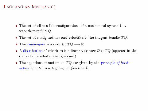
Lagrangian Mechanics
The set of all possible con�gurations of a mechanical system is a
smooth manifold Q.
The set of con�gurations and velocities is the tangent bundle TQ.
The Lagrangian is a map L : TQ −→ R
A distribution of velocities is a linear subspace D ⊂ TQ (appears in the
context of nonholonomic systems.)
The equations of motion on TQ are given by the principle of least
action applied to a Lagrangian function L.
Symmetry
The Lagrangian function is invariant under a Lie group action
L(g · q) = L(q) ∀q ∈ TQ,∀g ∈ G,
where G is a Lie group.

Lagrangian reduction
By identifying the group symmetry and utilizing the associated
conservation law, the dynamics are expressed on a reduced space.
Start with Q, de�ne a Lie group G action. If the Lagrangian and
distribution are invariant with respect to this group action, express the
reduced Lagrangian on TQ/G 1.
Factor the symmetry on the semidirect product (Euclidean space) to
obtain the Euler-Poincaré equation on reduced space 2.
1Bloch, AM, Krishnaprasad PS, Marsden JE and Murray RM: Archive for Rational
Mechanics and Anal.,136, pp 21-99, 1996.2Cendra H, Holm DD, Marsden JE and Ratiu TS : AMS Trans.(2), vol.186, 1998.

Symmetry Breaking
The full Lie group symmetry is sometimes broken - results in an
isotropy subgroup (eg. with a gravity term).
The Lagrangian function's G-invariance is now expressed with an
advected parameter. (the terminology "advected" �nds its source in
�uid modeling as invariants of a �ow .3)
The equation of motion on a reduced space, given by the principle of
least action on a reduced Lagrangian function l, is called the
Euler-Poincaré equation (EP).
The Euler-Poincaré framework for the Chaplygin's sphere where the center
of mass coincides with the geometric center of the sphere has been
discussed by Schneider4.
3D. D. Holm al: Geometric Mechanics and Symmetry, Oxford Texts, 2009.4Schneider D:Dynamical Systems, pp 87-130, 2002.

The Euler-Poincaré equation - with potential energy terms
Start with the extended con�guration space Q and the associated
Lagrangian L, which is assumed invariant under G.
System con�guration Q is an immersed submanifold of Q and the
system Lagrangian is invariant under the isotropy subgroup - Gk .
The velocity constraints expressed as a distribution - D ⊂ TQ - give
rise to a reduced constrained-Lagrangian.
Incorporating the advection dynamics, we obtain the Euler-Poincaré
equation.

Outline
Introduction
The Setting
Modeling of spherical robot
Dynamic equation
Equilibrium Configuration
Controllability
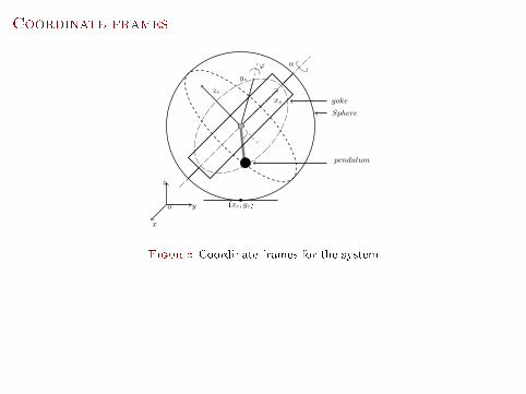
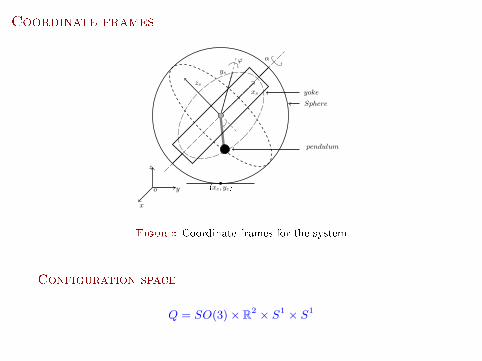
Coordinate frames
o y
z
x
(xc, yc)
xs
zs
ys
ϕ
yoke
Sphere
pendulum
α
Figure: Coordinate frames for the system
Configuration space
Q = SO(3)× R2 × S1 × S1
Coordinate frames
o y
z
x
(xc, yc)
xs
zs
ys
ϕ
yoke
Sphere
pendulum
α
Figure: Coordinate frames for the system
Configuration space
Q = SO(3)× R2 × S1 × S1

Notations
Rs ∈ SO(3)- orientation of the sphere with respect to the inertial
frame,
Rα - orientation of the yoke with respect to the sphere body frame,
Rϕ - orientation of the pendulum with respect to the yoke frame,
(ωs)s, (ωα)Y , (ωϕ)P - angular velocity of sphere in sphere frame,
angular velocity of yoke in yoke frame and angular velocity of
pendulum in pendulum body frame respectively.
rs -linear velocity of the centre of mass of the sphere.

Lagrangian
L =1
2ms‖rs‖2 +
1
2〈Iωss , ωss〉︸ ︷︷ ︸
K.E.ofsphere
+mpgl〈e3, RsRαRϕkp〉︸ ︷︷ ︸P.E.ofpendulum
+1
2mp‖rs + [Rsω
ss +RsRα(ωα)Y +RsRαRϕ(ωϕ)P ]×RsRαRϕkp‖2︸ ︷︷ ︸
K.E.ofpendulum
Rolling constraint: rs = (ωs)I × re3 =⇒ rs = (ωs)
Ire3
Symmetry
Left group action, G = SO(3) n R3 on manifold Q.
L and D are invariant when RT1 e3 = e3. (Remain unchanged if we
translate the inertial frame anywhere on the XY-plane and rotate it
about e3, the direction of gravity.)
Symmetry group
Ge3 = {(Rs, b) ∈ SO(3) n R3|RTs e3 = e3} = SO(2) n R2.
The advected quantity here is Γ(t) = RTs e3

Mappings
Adjoint and Co-Adjoint operation for SE(3) = SO(3)nR3
Ad(R,x)(ξ, υ) =(RξR−1, Rυ −RξR−1x
)Ad∗(R,x)−1(µ, β) = (RµR−1 + x � (Rβ), Rβ)
where (ξ, υ) ∈ se(3) = so(3) n R3, (µ, β) ∈ se∗(3) = so∗(3) n (R3)∗. Rβ
denote the induced left action of R on β i.e. the left action of SO(3) on
R3 induces a left action of SO(3) on (R3)∗.
Adjoint and Co-adjoint action of se(3) = so(3)nR3
ad(η,ν)(ξ, υ) = ([η, ξ], ηυ − ξν)
where induced action of so(3) on R3 is denoted by ην.
ad∗(η,ν)(µ, β) = (−[η, µ] + β � ν,−ηβ) .

Lagrangian reduction
Con�guration space S = SO(3) n R3 × S1 × S1
Original Lagrangian L : T (SO(3)× R2 × S1 × S1) −→ R
Reduced Lagrangian l : t×M × S1 × S1 −→ R t ∈ so(3)× R3
Constrained Lagrangian lc : h×M × S1 × S1 −→ R h ∈ so(3)
M is the orbit space of G/Ge3 acting on e3 in R3.
L(Rs, e3, Rs, X, Rα,Rϕ, Rα, Rϕ)
= l(e,RTs Rs, RTs X, R
Ts e3, Rα, Rϕ, Rα, Rϕ),
= l(ωss , Y ,Γ, Rα, Rϕ, Rα, Rϕ),
= lc(ωss , rω
ssΓ,Γ, Rα, Rϕ, Rα, Rϕ).
Rolling constraint Y = rωssΓ.
ωss = RTs Rs is the (left-invariant) sphere-body angular velocity.

Outline
Introduction
The Setting
Modeling of spherical robot
Dynamic equation
Equilibrium Configuration
Controllability

The Euler-Poincaré equation
ddt
(∂lc∂ωs
s
)− ad∗ωs
s
(∂lc∂ωs
s
)= −
(∂l∂Y� Γ)
+(∂l∂Γ� Γ),
d
dt
(∂l
∂α
)− ∂l
∂α= 0,
d
dt
(∂l
∂ϕ
)− ∂l
∂ϕ= 0,
Γ = −ωss × Γ.
The diamond operator
ρv : so(3)→R3 ρ∗v : so∗(3)→R3∗
R3 × R3∗→ so∗(3) : (v, w)→ v � w 4= ρ∗v(w)
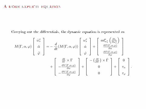
A more explicit equation
Carrying out the di�erentials, the dynamic equation is represented as
M(Γ, α, ϕ)
ωss
α
ϕ
=− d
dt(M(Γ, α, ϕ))
ωss
α
ϕ
+
ad∗ωs
s
(∂lc∂ωs
s
)∂T (Γ,α,ϕ)
∂α
∂T (Γ,α,ϕ)∂ϕ
+
∂lδΓ× Γ
− ∂V (Γ,α,ϕ)∂α
− ∂V (Γ,α,ϕ)∂ϕ
+
−(∂l∂Y
)× Γ
0
0
+
0
τα
τϕ
.

Outline
Introduction
The Setting
Modeling of spherical robot
Dynamic equation
Equilibrium Configuration
Controllability
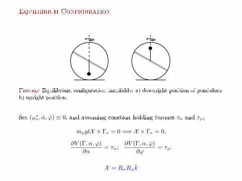
Equilibrium Configuration
Figure: Equilibrium con�guration manifolds: a) downright position of pendulum
b) upright position.
Set (ωss , α, ϕ) ≡ 0, and assuming constant holding torques τα and τϕ,
mpglX × Γe = 0 =⇒ X × Γe = 0,
∂V (Γ, α, ϕ)
∂α= τα;
∂V (Γ, α, ϕ)
∂ϕ= τϕ.
X = RαRϕk

Observations on equilibria
Vector X is collinear with the gravity vector RTs e3 in sphere-body
frame.
Fix α, ϕ: all con�gurations obtained by a rotation around the vertical
axis passing through the point of contact, constitute the equilibrium
manifold.
If Rse is an arbitrary orientation, then any α & ϕ such that X is in the
downright or upright position constitutes an equilibrium.
The control equilibrium of the reduced system is given as
{(Rs, α, ϕ)|Γ×X = 0} ⇒ {(Rs, α, ϕ)|RαRϕ = RTs }
where Γ = RTs e3 and X = RαRϕk.

Outline
Introduction
The Setting
Modeling of spherical robot
Dynamic equation
Equilibrium Configuration
Controllability

Vector fields on the reduced space
The control vector �elds on the reduced space T (SO(3)× S1 × S1) are
Yi = M−1(Γ, α, ϕ)
[0
yi
]The potential vector �eld on the reduced space T (SO(3)× S1 × S1) is
(gradV )˜ = M−1(Γ, α, ϕ)
[mpgΓ×X
0
]
where i = α,ϕ and yi is a T∗(S1 × S1)-valued function.

Computational procedure
Calculate the symmetric product⟨Yi : Yj
⟩.
Evaluate the iterated symmetric product of Sym(Y) = {Y ∪ (gradV )˜}.
The system is local con�guration accessible at equilibrium if the rank
of Lie(Sym(Y)) = dim(Q) at q0.
Every bad symmetric product from {Y ∪ (gradV )˜} is the linearcombination of lower degree good symmetric products, then the system
is small time local con�guration controllable.

References
1 D. Schneider, Non-holonomic Euler-Poincaré equations and stability in
Chaplygin's sphere,Dynamical Systems, 2002, pp.87-130
2 A. M. Bloch.Nonholonomic Mechanics and Control . New York:
Springer-Verlag, 2003
3 Bloch, A. M, krishnaprasad P. S, Marsden J. E and Murray R. M. ,
Nonholonomic mechanical systems with symmetry. Archive for
Rational Mechanics and Analysis, 1996, volume 136 pp 21-99.
4 Holm, D. D, Schmah, T and Stoica, C.Geometric Mechanics and
Symmetry, Oxford University Press Inc., New York, 2009.
5 Cendra H, Holm D. D, Marsden J. E and Ratiu T. S Lagrangian
reduction, the Euler-Poincaré equations, and semidirect products,
American Mathematical Society Translation(2), 1998, Volume 186
6 D. D. Holm, Geometric Mechanics: Rotating, Translating and Rolling,
Imperial College Press, 2008

THANK YOU