the equatorial subthermocline … equatorial subthermocline circulation in observations ... ocean...

THE EQUATORIAL SUBTHERMOCLINE

CIRCULATION IN OBSERVATIONS

Francois Ascani

September 24, 2009

Contents

0.1 Observations . . . . . . . . . . . . . . . . . . . . . . . . . . . . . . . . . . . . 60.1.1 Indian Ocean . . . . . . . . . . . . . . . . . . . . . . . . . . . . . . . 60.1.2 Pacific Ocean . . . . . . . . . . . . . . . . . . . . . . . . . . . . . . . 7

1 Results 9

1.1 Observations . . . . . . . . . . . . . . . . . . . . . . . . . . . . . . . . . . . . 91.1.1 Indian Ocean . . . . . . . . . . . . . . . . . . . . . . . . . . . . . . . 91.1.2 Pacific Ocean - Residual . . . . . . . . . . . . . . . . . . . . . . . . . 17

A Plate Indian Ocean 21

B Plate Pacific Ocean 34

1

List of Tables

1 Hydrographic and velocity data sources in the Indian Ocean between 5◦Sand 5◦N; LADCP NB, Lowered Acoustic Doppler Current Profiler, 300 kHz,narrow bandwidth; LADCP BB, Lowered Acoustic Doppler Current Profiler,150 kHz, broad bandwidth. . . . . . . . . . . . . . . . . . . . . . . . . . . . . 7

2 Hydrographic and velocity data sources in the Pacific Ocean between 4◦Sand 4◦N; LADCP NB, Lowered Acoustic Doppler Current Profiler, 300 kHz,narrow bandwidth; LADCP BB, Lowered Acoustic Doppler Current Profiler,150 kHz, broad bandwidth. . . . . . . . . . . . . . . . . . . . . . . . . . . . . 8

2

List of Figures

1 Locations of current measurements. Only those within 5◦ of the equator arediscussed here. I7N, I7NR(1), I7NR(2), I8N, I8NR and I9N refer to WorldOcean Circulation Experiment Hydrographic Project survey lines. See Table1 for details. . . . . . . . . . . . . . . . . . . . . . . . . . . . . . . . . . . . . 6

2 Locations of current measurements. Only those within 4◦ of the equator arediscussed here. P10, P13, P14, P16, P17, P18, and P19 refer to World OceanCirculation Experiment Hydrographic Project survey lines. See Table 2 fordetails. . . . . . . . . . . . . . . . . . . . . . . . . . . . . . . . . . . . . . . . 8

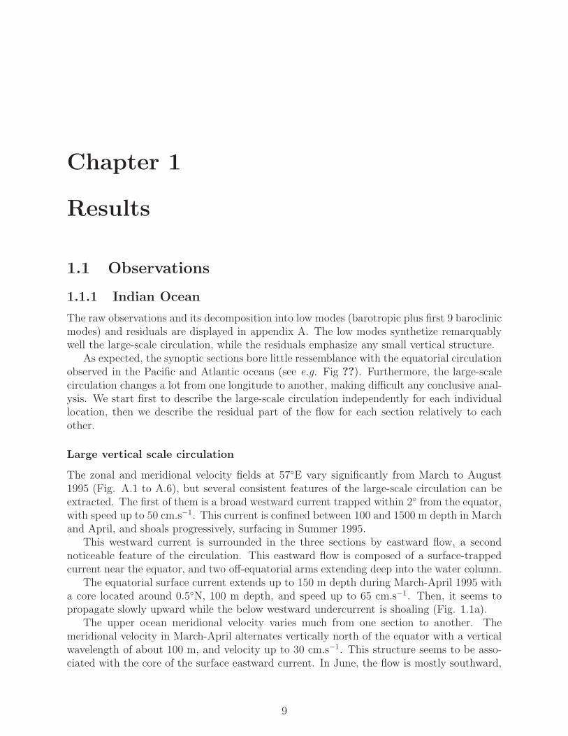
1.1 Low mode zonal velocity U averaged within 1.5◦ from the equator. The lowmodes are represented by the barotropic and first 9 baroclinic modes. . . . . 10

1.2 Wind at 10 m above the surface from NCEP Reanalysis-2 along the equator,during the year covering the cruise observations (located by symbols). . . . . 11

1.3 Amplitudes squared of the vertical modes associated with the zonal velocityU, and averaged within 1◦ from the equator. Note the different vertical scalesbetween each panel. Mode 9 is adequate to separate the high from the lowmodes. . . . . . . . . . . . . . . . . . . . . . . . . . . . . . . . . . . . . . . . 12

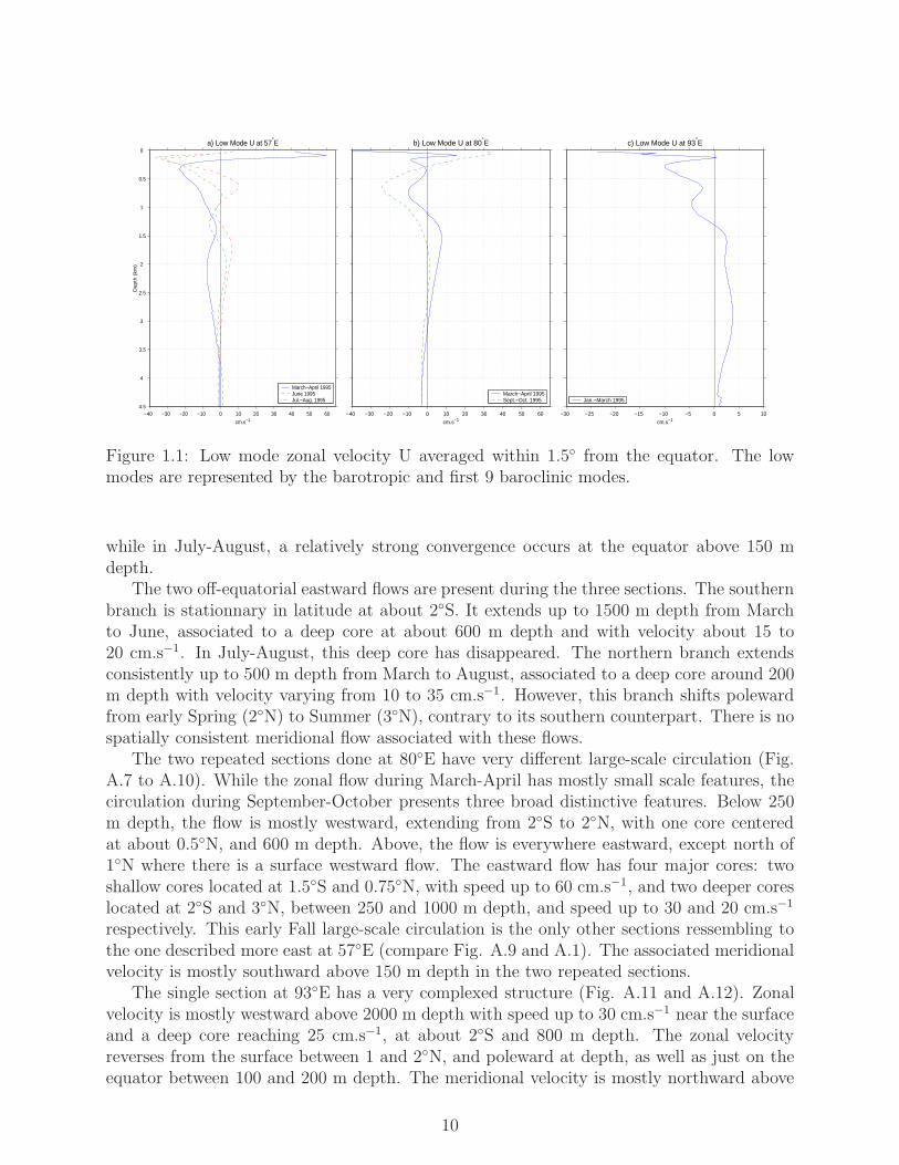
1.4 Residual zonal velocity U averaged within 1◦ from the equator. . . . . . . . . 131.5 Energy density spectrum versus stretched vertical wavelength and latitude

for each section. The residuals have been masked between 500 and 3000 mdepth, then WKB stretched and scaled (with N

s= 1 cph) before Fourier

decomposition. In each panel, the right axis shows the pair of vertical modesequivalent for each wavelength, and the top axis shows the actual latitudes ofobservations. . . . . . . . . . . . . . . . . . . . . . . . . . . . . . . . . . . . . 14

3

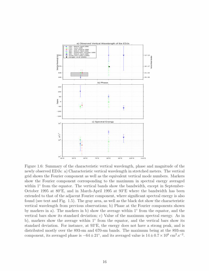
1.6 Summary of the characteristic vertical wavelength, phase and magnitude ofthe newly observed EDJs: a) Characteristic vertical wavelength in stretchedmeters. The vertical grid shows the Fourier component as well as the equiva-lent vertical mode numbers. Markers show the Fourier component correspond-ing to the maximum in spectral energy averaged within 1◦ from the equator.The vertical bands show the bandwidth, except in September-October 1995at 80◦E, and in March-April 1995 at 93◦E where the bandwidth has been ex-tended to that of the adjacent Fourier component, where significant spectralenergy is also found (see text and Fig. 1.5). The gray area, as well as the blackdot show the characteristic vertical wavelength from previous observations; b)Phase at the Fourier components shown by markers in a). The markers inb) show the average within 1◦ from the equator, and the vertical bars showits standard deviation; c) Value of the maximum spectral energy. As in b),markers show the average within 1◦ from the equator, and the vertical barsshow its standard deviation. For instance, at 93◦E, the energy does not have astrong peak, and is distributed mostly over the 893-sm and 670-sm bands. Themaximum being at the 893-sm component, its averaged phase is −64 ± 21◦,and its averaged value is 14 ± 0.7 × 108 cm2.s−2. . . . . . . . . . . . . . . . . 16

1.7 Amplitudes squared of the vertical modes associated with the zonal velocityU, and averaged within 1◦ from the equator. Note the different vertical scalesbetween each panel. Mode 10 is adequate to separate the high from the lowmodes. . . . . . . . . . . . . . . . . . . . . . . . . . . . . . . . . . . . . . . . 17

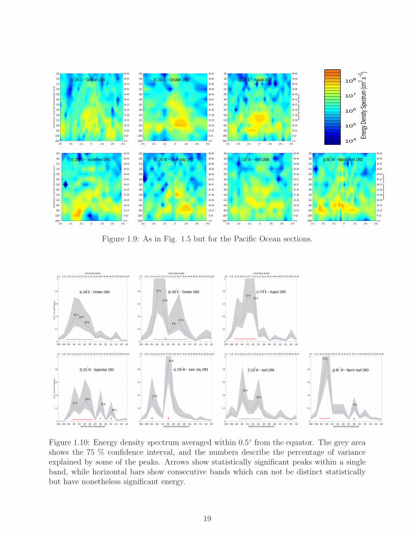
1.8 Residual zonal velocity U averaged within 1◦ from the equator. . . . . . . . . 181.9 As in Fig. 1.5 but for the Pacific Ocean sections. . . . . . . . . . . . . . . . 191.10 Energy density spectrum averaged within 0.5◦ from the equator. The grey area

shows the 75 % confidence interval, and the numbers describe the percentage ofvariance explained by some of the peaks. Arrows show statistically significantpeaks within a single band, while horizontal bars show consecutive bandswhich can not be distinct statistically but have nonetheless significant energy. 19

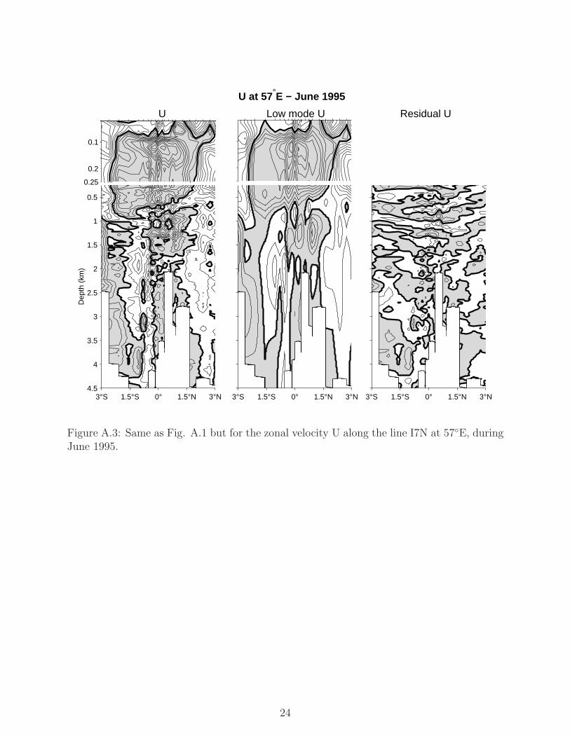
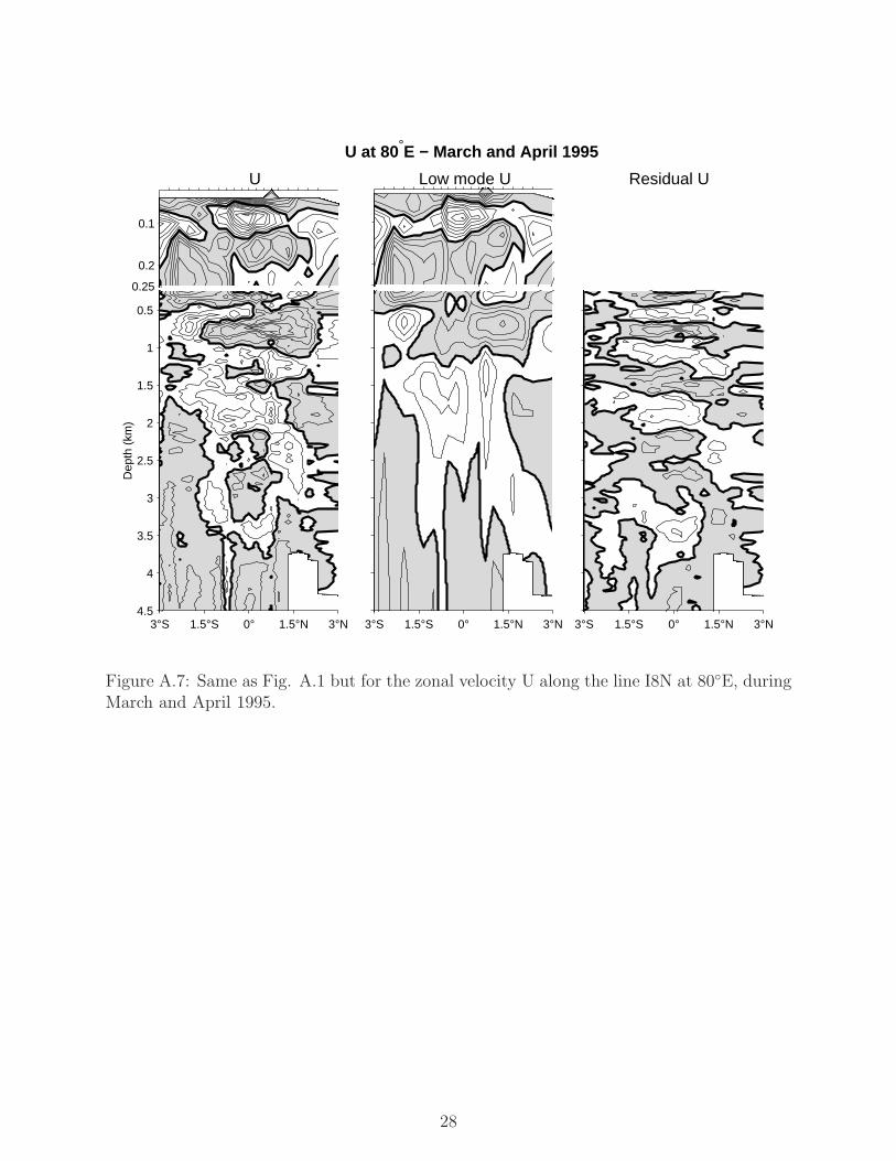
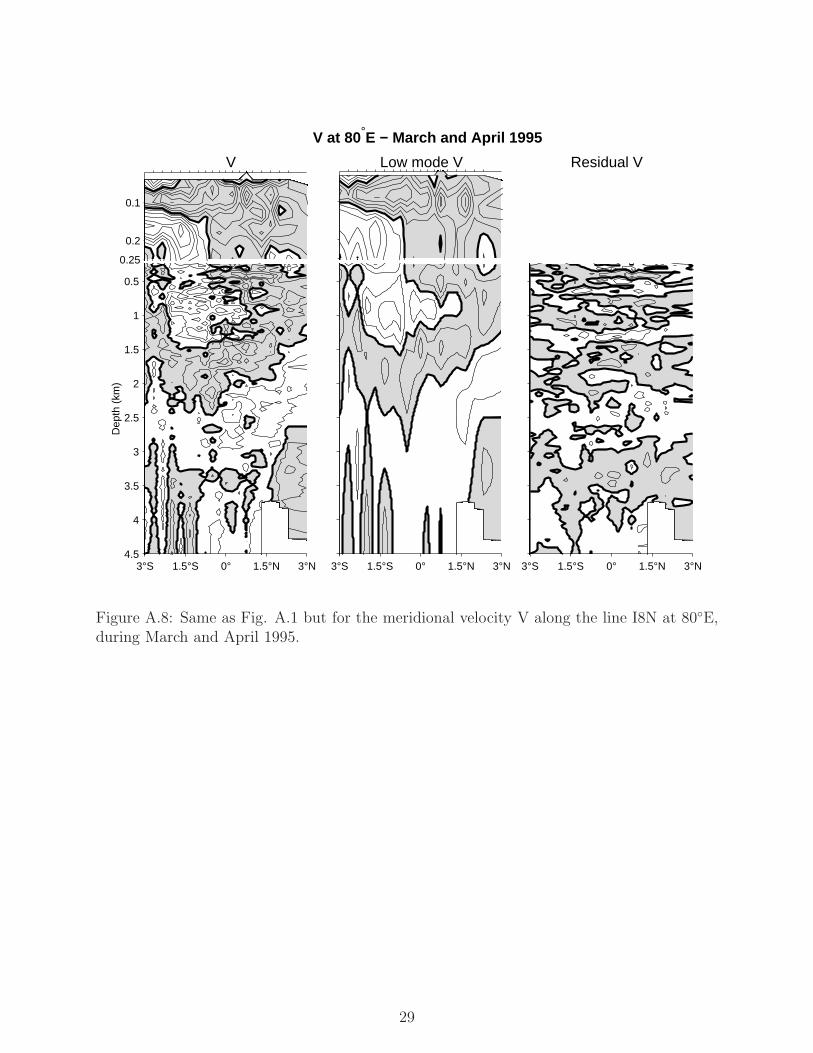
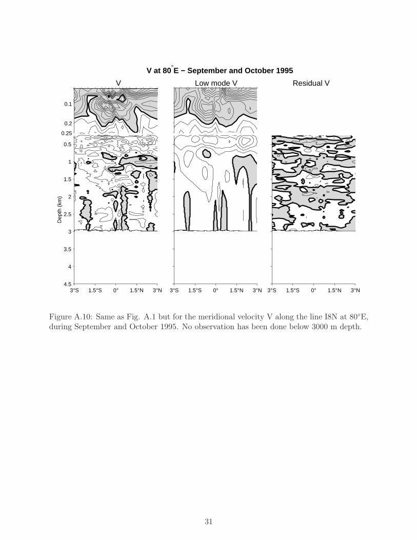
A.1 Zonal velocity U along the line I7N at 57◦E, during March and April 1995.The left panels show the full velocity, the middle panels show the low modes(barotropic plus first 9 baroclinic modes), and the right panel shows the resid-ual. The top panels show the top 250 m. This decomposition has been donewithout masking the upper 5000 and lower 3000 m depth. Especially, thetop 250 m of the residual is polluted by mathematical artifacts from the de-composition, and is not shown. Contour intervals are each 5 cm.s−1. Shadedareas indicate negative values. Tick marks on top axis indicate the latitudesof observations. . . . . . . . . . . . . . . . . . . . . . . . . . . . . . . . . . . 22

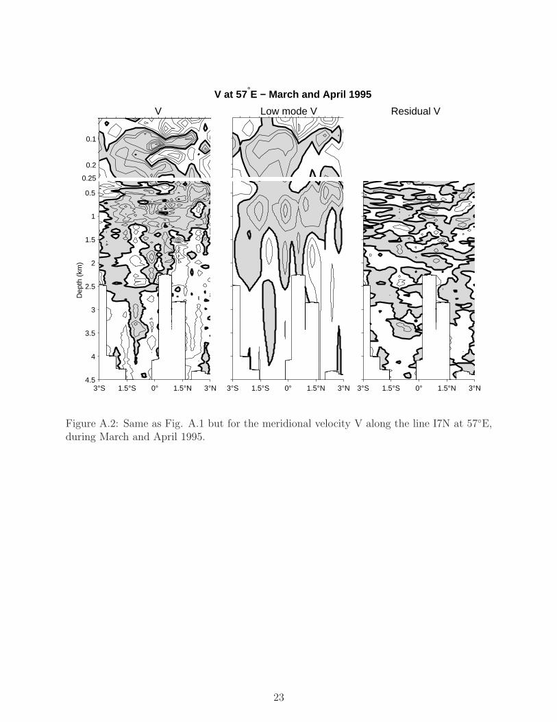
A.2 Same as Fig. A.1 but for the meridional velocity V along the line I7N at 57◦E,during March and April 1995. . . . . . . . . . . . . . . . . . . . . . . . . . . 23

A.3 Same as Fig. A.1 but for the zonal velocity U along the line I7N at 57◦E,during June 1995. . . . . . . . . . . . . . . . . . . . . . . . . . . . . . . . . . 24

A.4 Same as Fig. A.1 but for the meridional velocity V along the line I7N at 57◦E,during June 1995. . . . . . . . . . . . . . . . . . . . . . . . . . . . . . . . . . 25

4

A.5 Same as Fig. A.1 but for the zonal velocity U along the line I7N at 57◦E,during July and August 1995. . . . . . . . . . . . . . . . . . . . . . . . . . . 26

A.6 Same as Fig. A.1 but for the meridional velocity V along the line I7N at 57◦E,during July and August 1995. . . . . . . . . . . . . . . . . . . . . . . . . . . 27

A.7 Same as Fig. A.1 but for the zonal velocity U along the line I8N at 80◦E,during March and April 1995. . . . . . . . . . . . . . . . . . . . . . . . . . . 28

A.8 Same as Fig. A.1 but for the meridional velocity V along the line I8N at 80◦E,during March and April 1995. . . . . . . . . . . . . . . . . . . . . . . . . . . 29

A.9 Same as Fig. A.1 but for the zonal velocity U along the line I8N at 80◦E,during September and October 1995. No observation has been done below3000 m depth. . . . . . . . . . . . . . . . . . . . . . . . . . . . . . . . . . . . 30

A.10 Same as Fig. A.1 but for the meridional velocity V along the line I8N at80◦E, during September and October 1995. No observation has been donebelow 3000 m depth. . . . . . . . . . . . . . . . . . . . . . . . . . . . . . . . 31

A.11 Same as Fig. A.1 but for the zonal velocity U along the line I9N at 93◦E,during January and April 1995. . . . . . . . . . . . . . . . . . . . . . . . . . 32

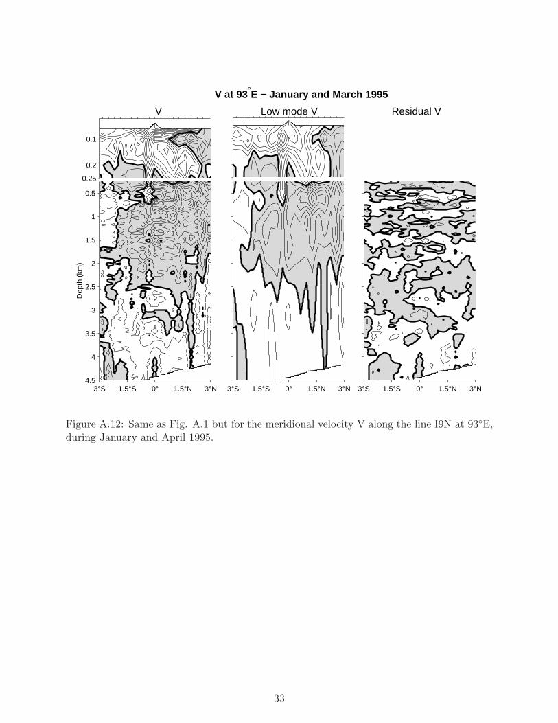
A.12 Same as Fig. A.1 but for the meridional velocity V along the line I9N at 93◦E,during January and April 1995. . . . . . . . . . . . . . . . . . . . . . . . . . 33

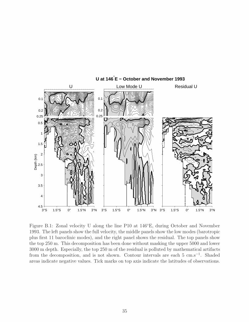
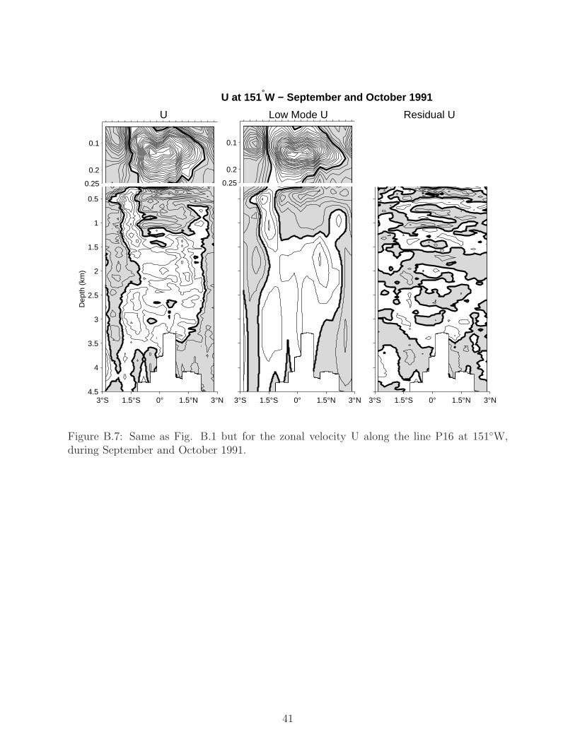
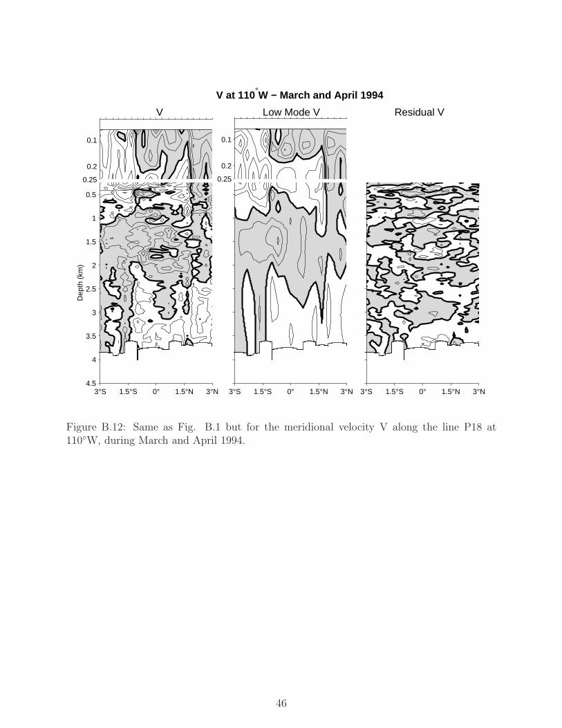
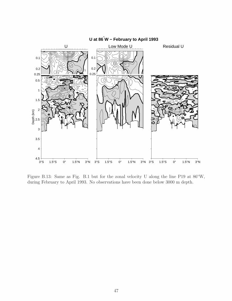
B.1 Zonal velocity U along the line P10 at 146◦E, during October and November1993. The left panels show the full velocity, the middle panels show the lowmodes (barotropic plus first 11 baroclinic modes), and the right panel showsthe residual. The top panels show the top 250 m. This decomposition has beendone without masking the upper 5000 and lower 3000 m depth. Especially,the top 250 m of the residual is polluted by mathematical artifacts from thedecomposition, and is not shown. Contour intervals are each 5 cm.s−1. Shadedareas indicate negative values. Tick marks on top axis indicate the latitudesof observations. . . . . . . . . . . . . . . . . . . . . . . . . . . . . . . . . . . 35

B.2 Same as Fig. B.1 but for the meridional velocity V along the line P10 at146◦E, during October and November 1993. . . . . . . . . . . . . . . . . . . 36

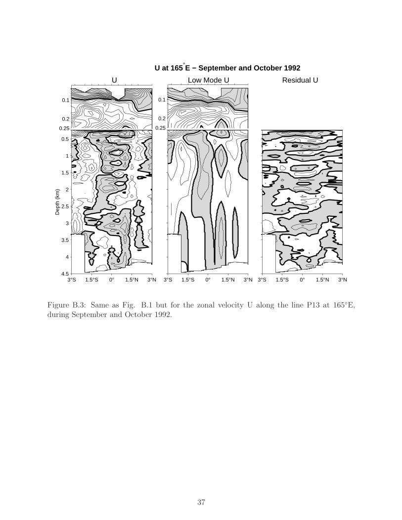
B.3 Same as Fig. B.1 but for the zonal velocity U along the line P13 at 165◦E,during September and October 1992. . . . . . . . . . . . . . . . . . . . . . . 37

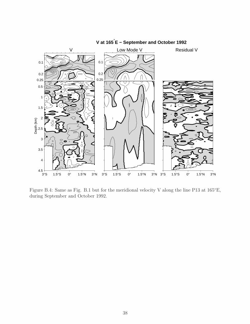
B.4 Same as Fig. B.1 but for the meridional velocity V along the line P13 at165◦E, during September and October 1992. . . . . . . . . . . . . . . . . . . 38

B.5 Same as Fig. B.1 but for the zonal velocity U along the line P14 at 179◦E,during August 1993. . . . . . . . . . . . . . . . . . . . . . . . . . . . . . . . 39

B.6 Same as Fig. B.1 but for the meridional velocity V along the line P14 at179◦E, during August 1993. . . . . . . . . . . . . . . . . . . . . . . . . . . . 40

B.7 Same as Fig. B.1 but for the zonal velocity U along the line P16 at 151◦W,during September and October 1991. . . . . . . . . . . . . . . . . . . . . . . 41

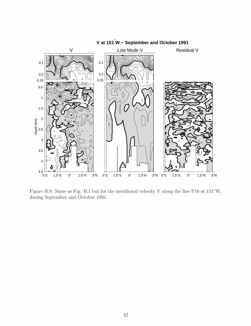
B.8 Same as Fig. B.1 but for the meridional velocity V along the line P16 at151◦W, during September and October 1991. . . . . . . . . . . . . . . . . . . 42

B.9 Same as Fig. B.1 but for the zonal velocity U along the line P17 at 135◦W,during May and July 1991. . . . . . . . . . . . . . . . . . . . . . . . . . . . . 43

5

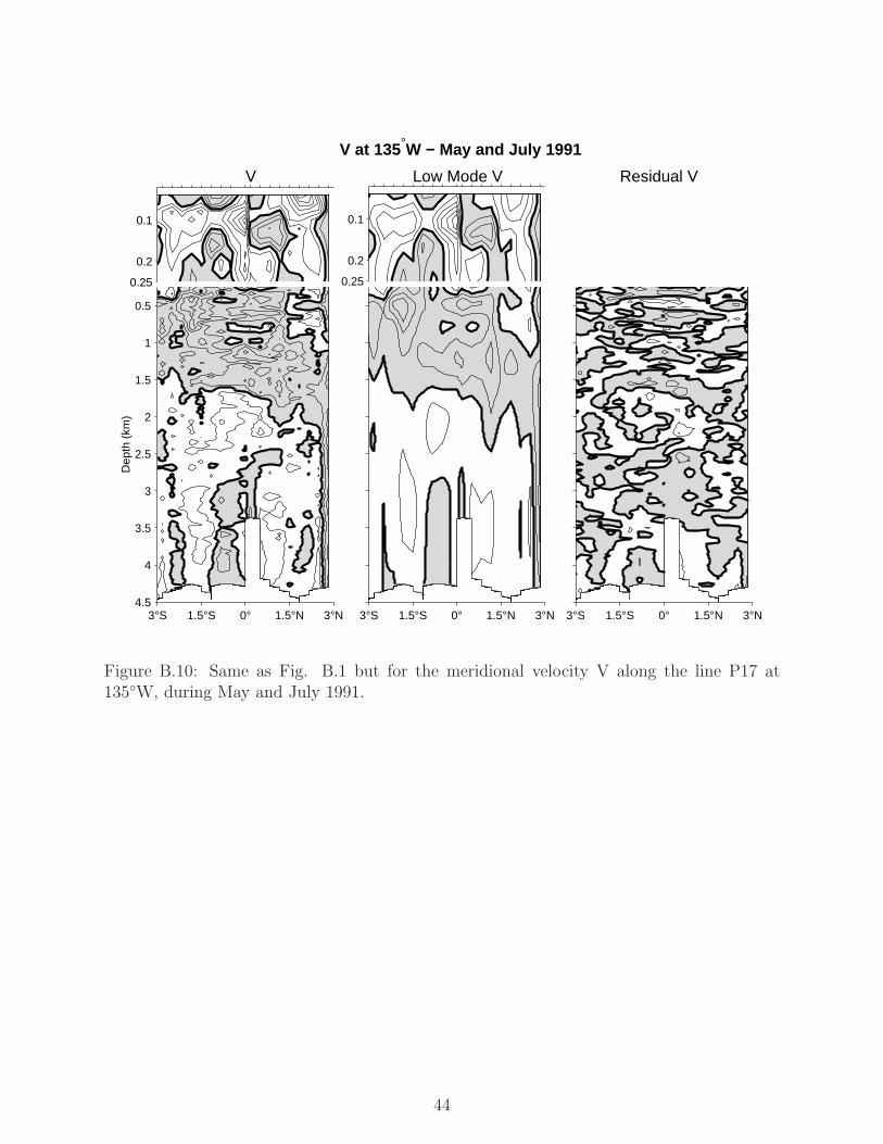
B.10 Same as Fig. B.1 but for the meridional velocity V along the line P17 at135◦W, during May and July 1991. . . . . . . . . . . . . . . . . . . . . . . . 44

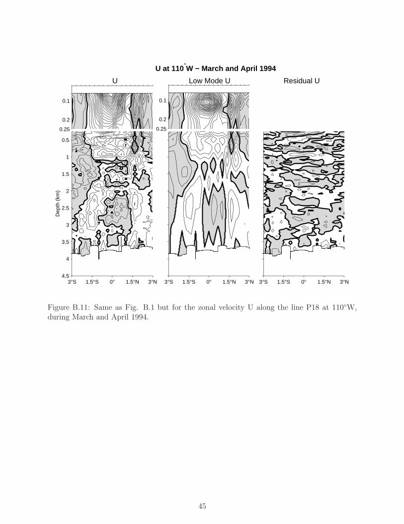
B.11 Same as Fig. B.1 but for the zonal velocity U along the line P18 at 110◦W,during March and April 1994. . . . . . . . . . . . . . . . . . . . . . . . . . . 45

B.12 Same as Fig. B.1 but for the meridional velocity V along the line P18 at110◦W, during March and April 1994. . . . . . . . . . . . . . . . . . . . . . . 46

B.13 Same as Fig. B.1 but for the zonal velocity U along the line P19 at 86◦W,during February to April 1993. No observations have been done below 3000m depth. . . . . . . . . . . . . . . . . . . . . . . . . . . . . . . . . . . . . . . 47

B.14 Same as Fig. B.1 but for the meridional velocity V along the line P19 at86◦W, during February to April 1993. No observations have been done below3000 m depth. . . . . . . . . . . . . . . . . . . . . . . . . . . . . . . . . . . . 48

0.1 Observations

0.1.1 Indian Ocean

Very few observations of the deep equatorial Indian Ocean are available (see e.g. Schott andMcCreary 2001). The subthermocline part of observations done during the year 1995, aspart of the World Ocean Circulation Experiment (WOCE) Hydrographic Project (WHP),are presented here for the first time.

Hydrographic and current profile measurements were carried out along three meridionallines in the Indian Ocean (Fig. 1), using a Lowered Acoustic Data Current Profiler (LADCP)mounted on the rosette with the CTD, profiling the full velocity field from the surface up tothe bottom.

Depth (km)1 2 3 4 5

40°E 50°E 60°E 70°E 80°E 90°E 100°E 110°E

10°S

5°S

0°

5°N

10°N I7N

I7NR(1) I7NR(2) I8N

I8NR

I9N

Figure 1: Locations of current measurements. Only those within 5◦ of the equator arediscussed here. I7N, I7NR(1), I7NR(2), I8N, I8NR and I9N refer to World Ocean CirculationExperiment Hydrographic Project survey lines. See Table 1 for details.

The line I7N is located in the western Indian Ocean, and was completed by R/V Knorr

cruise 145/10 between July and August 1995. It crosses the equator at about 57◦E. Thisline has been revisited by R/V Malcolm Baldrige cruise MB95-02 (section I7NR1) between

6

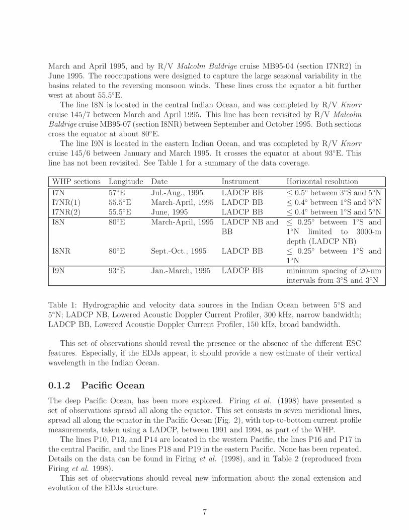
March and April 1995, and by R/V Malcolm Baldrige cruise MB95-04 (section I7NR2) inJune 1995. The reoccupations were designed to capture the large seasonal variability in thebasins related to the reversing monsoon winds. These lines cross the equator a bit furtherwest at about 55.5◦E.

The line I8N is located in the central Indian Ocean, and was completed by R/V Knorr

cruise 145/7 between March and April 1995. This line has been revisited by R/V Malcolm

Baldrige cruise MB95-07 (section I8NR) between September and October 1995. Both sectionscross the equator at about 80◦E.

The line I9N is located in the eastern Indian Ocean, and was completed by R/V Knorr

cruise 145/6 between January and March 1995. It crosses the equator at about 93◦E. Thisline has not been revisited. See Table 1 for a summary of the data coverage.

WHP sections Longitude Date Instrument Horizontal resolution

I7N 57◦E Jul.-Aug., 1995 LADCP BB ≤ 0.5◦ between 3◦S and 5◦NI7NR(1) 55.5◦E March-April, 1995 LADCP BB ≤ 0.4◦ between 1◦S and 5◦NI7NR(2) 55.5◦E June, 1995 LADCP BB ≤ 0.4◦ between 1◦S and 5◦NI8N 80◦E March-April, 1995 LADCP NB and

BB≤ 0.25◦ between 1◦S and1◦N limited to 3000-mdepth (LADCP NB)

I8NR 80◦E Sept.-Oct., 1995 LADCP BB ≤ 0.25◦ between 1◦S and1◦N

I9N 93◦E Jan.-March, 1995 LADCP BB minimum spacing of 20-nmintervals from 3◦S and 3◦N

Table 1: Hydrographic and velocity data sources in the Indian Ocean between 5◦S and5◦N; LADCP NB, Lowered Acoustic Doppler Current Profiler, 300 kHz, narrow bandwidth;LADCP BB, Lowered Acoustic Doppler Current Profiler, 150 kHz, broad bandwidth.

This set of observations should reveal the presence or the absence of the different ESCfeatures. Especially, if the EDJs appear, it should provide a new estimate of their verticalwavelength in the Indian Ocean.

0.1.2 Pacific Ocean

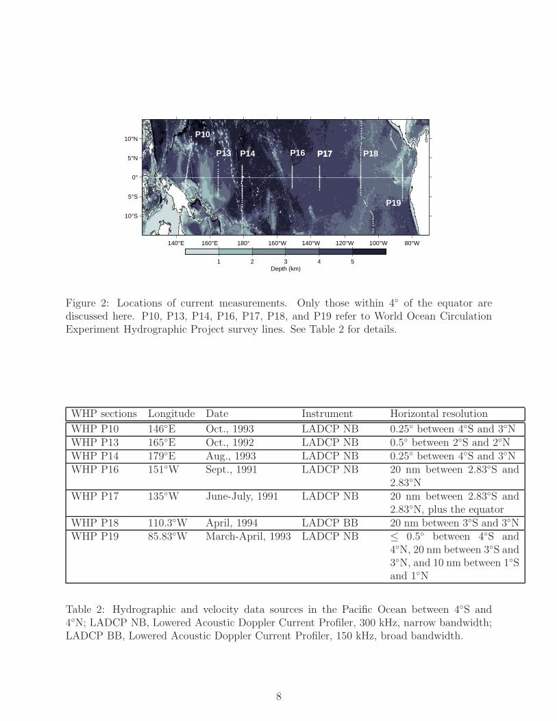
The deep Pacific Ocean, has been more explored. Firing et al. (1998) have presented aset of observations spread all along the equator. This set consists in seven meridional lines,spread all along the equator in the Pacific Ocean (Fig. 2), with top-to-bottom current profilemeasurements, taken using a LADCP, between 1991 and 1994, as part of the WHP.

The lines P10, P13, and P14 are located in the western Pacific, the lines P16 and P17 inthe central Pacific, and the lines P18 and P19 in the eastern Pacific. None has been repeated.Details on the data can be found in Firing et al. (1998), and in Table 2 (reproduced fromFiring et al. 1998).

This set of observations should reveal new information about the zonal extension andevolution of the EDJs structure.

7

Depth (km)1 2 3 4 5

140°E 160°E 180° 160°W 140°W 120°W 100°W 80°W

10°S

5°S

0°

5°N

10°NP10

P13 P14 P16 P17 P17 P18

P19

Figure 2: Locations of current measurements. Only those within 4◦ of the equator arediscussed here. P10, P13, P14, P16, P17, P18, and P19 refer to World Ocean CirculationExperiment Hydrographic Project survey lines. See Table 2 for details.

WHP sections Longitude Date Instrument Horizontal resolution

WHP P10 146◦E Oct., 1993 LADCP NB 0.25◦ between 4◦S and 3◦NWHP P13 165◦E Oct., 1992 LADCP NB 0.5◦ between 2◦S and 2◦NWHP P14 179◦E Aug., 1993 LADCP NB 0.25◦ between 4◦S and 3◦NWHP P16 151◦W Sept., 1991 LADCP NB 20 nm between 2.83◦S and

2.83◦NWHP P17 135◦W June-July, 1991 LADCP NB 20 nm between 2.83◦S and

2.83◦N, plus the equatorWHP P18 110.3◦W April, 1994 LADCP BB 20 nm between 3◦S and 3◦NWHP P19 85.83◦W March-April, 1993 LADCP NB ≤ 0.5◦ between 4◦S and

4◦N, 20 nm between 3◦S and3◦N, and 10 nm between 1◦Sand 1◦N

Table 2: Hydrographic and velocity data sources in the Pacific Ocean between 4◦S and4◦N; LADCP NB, Lowered Acoustic Doppler Current Profiler, 300 kHz, narrow bandwidth;LADCP BB, Lowered Acoustic Doppler Current Profiler, 150 kHz, broad bandwidth.

8

Chapter 1

Results

1.1 Observations

1.1.1 Indian Ocean

The raw observations and its decomposition into low modes (barotropic plus first 9 baroclinicmodes) and residuals are displayed in appendix A. The low modes synthetize remarquablywell the large-scale circulation, while the residuals emphasize any small vertical structure.

As expected, the synoptic sections bore little ressemblance with the equatorial circulationobserved in the Pacific and Atlantic oceans (see e.g. Fig ??). Furthermore, the large-scalecirculation changes a lot from one longitude to another, making difficult any conclusive anal-ysis. We start first to describe the large-scale circulation independently for each individuallocation, then we describe the residual part of the flow for each section relatively to eachother.

Large vertical scale circulation

The zonal and meridional velocity fields at 57◦E vary significantly from March to August1995 (Fig. A.1 to A.6), but several consistent features of the large-scale circulation can beextracted. The first of them is a broad westward current trapped within 2◦ from the equator,with speed up to 50 cm.s−1. This current is confined between 100 and 1500 m depth in Marchand April, and shoals progressively, surfacing in Summer 1995.

This westward current is surrounded in the three sections by eastward flow, a secondnoticeable feature of the circulation. This eastward flow is composed of a surface-trappedcurrent near the equator, and two off-equatorial arms extending deep into the water column.

The equatorial surface current extends up to 150 m depth during March-April 1995 witha core located around 0.5◦N, 100 m depth, and speed up to 65 cm.s−1. Then, it seems topropagate slowly upward while the below westward undercurrent is shoaling (Fig. 1.1a).

The upper ocean meridional velocity varies much from one section to another. Themeridional velocity in March-April alternates vertically north of the equator with a verticalwavelength of about 100 m, and velocity up to 30 cm.s−1. This structure seems to be asso-ciated with the core of the surface eastward current. In June, the flow is mostly southward,

9

cm.s−1

De

pth

(km

)

a) Low Mode U at 57°E

−40 −30 −20 −10 0 10 20 30 40 50 604.5

4

3.5

3

2.5

2

1.5

1

0.5

0

March−April 1995June 1995Jul.−Aug. 1995

cm.s−1

b) Low Mode U at 80°E

−40 −30 −20 −10 0 10 20 30 40 50 60

March−April 1995Sept.−Oct. 1995

cm.s−1

c) Low Mode U at 93°E

−30 −25 −20 −15 −10 −5 0 5 10

Jan.−March 1995

Figure 1.1: Low mode zonal velocity U averaged within 1.5◦ from the equator. The lowmodes are represented by the barotropic and first 9 baroclinic modes.

while in July-August, a relatively strong convergence occurs at the equator above 150 mdepth.

The two off-equatorial eastward flows are present during the three sections. The southernbranch is stationnary in latitude at about 2◦S. It extends up to 1500 m depth from Marchto June, associated to a deep core at about 600 m depth and with velocity about 15 to20 cm.s−1. In July-August, this deep core has disappeared. The northern branch extendsconsistently up to 500 m depth from March to August, associated to a deep core around 200m depth with velocity varying from 10 to 35 cm.s−1. However, this branch shifts polewardfrom early Spring (2◦N) to Summer (3◦N), contrary to its southern counterpart. There is nospatially consistent meridional flow associated with these flows.

The two repeated sections done at 80◦E have very different large-scale circulation (Fig.A.7 to A.10). While the zonal flow during March-April has mostly small scale features, thecirculation during September-October presents three broad distinctive features. Below 250m depth, the flow is mostly westward, extending from 2◦S to 2◦N, with one core centeredat about 0.5◦N, and 600 m depth. Above, the flow is everywhere eastward, except north of1◦N where there is a surface westward flow. The eastward flow has four major cores: twoshallow cores located at 1.5◦S and 0.75◦N, with speed up to 60 cm.s−1, and two deeper coreslocated at 2◦S and 3◦N, between 250 and 1000 m depth, and speed up to 30 and 20 cm.s−1

respectively. This early Fall large-scale circulation is the only other sections ressembling tothe one described more east at 57◦E (compare Fig. A.9 and A.1). The associated meridionalvelocity is mostly southward above 150 m depth in the two repeated sections.

The single section at 93◦E has a very complexed structure (Fig. A.11 and A.12). Zonalvelocity is mostly westward above 2000 m depth with speed up to 30 cm.s−1 near the surfaceand a deep core reaching 25 cm.s−1, at about 2◦S and 800 m depth. The zonal velocityreverses from the surface between 1 and 2◦N, and poleward at depth, as well as just on theequator between 100 and 200 m depth. The meridional velocity is mostly northward above

10

250 m depth, and southward below.

50°E 55°E 60°E 65°E 70°E 75°E 80°E 85°E 90°E 95°E 100°ENov94

Dec94

Jan95

Feb95

Mar95

Apr95

May95

Jun95

Jul95

Aug95

Sep95

Oct95

Nov95NCEP2 10−m Wind

1 m.s−1

I7NI7NR(1)I7NR(2)I8NI8NRI9N

Figure 1.2: Wind at 10 m above the surface from NCEP Reanalysis-2 along the equator,during the year covering the cruise observations (located by symbols).

Previous observations have shown that the Indian Ocean has a strong semi-annual signal,characteristic of its wind forcing. Luyten and Roemmich (1982) observed upward propaga-tion of zonal velocity, characteristic of an eastward propagating equatorial Kelvin wave anda westward long equatorial Rossby wave. They estimated their vertical wavelength to be theocean depth that is about 5000 m. Can the observations at 57◦E and their apparent verti-cal propagation consistent with the wind forcing at that time as well as with the previousobservations ?

During the period of observations, the surface wind was close to its climatology (Fig. 1.2):northeasterly winds during the winter monsoon (January-February 1995), and southeasterlywinds during the summer monsoon (July-August 1995). Between each monsoon, in Apriland October 1995 , the winds were mostly eastward. Thus one can expect the wind to haveforced the previously observed semi-annual waves.

Unfortunately, the apparent vertical propagation at 57◦E can not be fitted by a singlewave. The low mode profiles between 500 and 4500 m depth are stretched and scaled beforebeing decomposed onto Fourier components. The most two recent profiles have a defined peakat 1820 sm (with N

s= 1 cph), while the earliest one has essentially a red spectrum. Knowing

the time difference between each profiles and using the 1820-sm spectral fit, one estimatethe possible periods of the single vertical propagation via phase difference. Looking at thelongest period, one find periods of 168 days (between March-April’s and June’s profiles), 353days (between June’s and July-August’s profiles), and 200 days (between March-April’s andJuly-August’s profiles). Another method via auto-correlation and lag-correlation betweenthe different profiles gives a similar broad estimate of the period, suggesting that severalwaves may contribute to the apparent vertical propagation.

11

In consequence, although the semi-annual period (about 182 days) is within the range ofthe above period estimations, the present observations can not permit to conclude on theexact nature of the visual vertical propagation at 57◦E.

Residual

We first take a look of the effect of the masking between 500 and 3000 m depth, and justifythe choice of vertical mode 9 as the limit between low modes and residual (Fig. 1.3).

cm

2.s

−2

Vertical Mode Number

a) 57°E − March−April 1995

0 2 4 6 8 10 12 14 16 18 20 22 24 26 28 300

10

20

30

40

50

60

70

80unmaskedmasked


b) 80°E − March−April 1995

0 2 4 6 8 10 12 14 16 18 20 22 24 26 28 300

5

10

15unmaskedmasked


c) 93°E − January−March 1995

0 2 4 6 8 10 12 14 16 18 20 22 24 26 28 300

5

10

15unmaskedmasked


cm

2.s

−2

d) 57°E − June 1995

0 2 4 6 8 10 12 14 16 18 20 22 24 26 28 300

5

10

15

20

25unmaskedmasked


e) 80°E − September−October 1995

0 2 4 6 8 10 12 14 16 18 20 22 24 26 28 300

10

20

30

40

50

60unmaskedmasked


cm

2.s

−2

f) 57°E − July−August 1995

0 2 4 6 8 10 12 14 16 18 20 22 24 26 28 300

2

4

6

8

10unmaskedmasked

Figure 1.3: Amplitudes squared of the vertical modes associated with the zonal velocity U,and averaged within 1◦ from the equator. Note the different vertical scales between eachpanel. Mode 9 is adequate to separate the high from the low modes.

The masking reduces very efficiently the energy of the low modes. It also reduces the“pollution” by strong vertical shear currents into the high modes which are our primaryinterest (see section ??). This is the case in the third section at 57◦E, in the first sectionat 80◦E, and at 93◦E. In these, subsequent energy is found at relatively moderate verticalmodes in the unmasked profiles (modes 8-14), which are spatially correlated with the lowestmodes (modes 0-7), and serve to reproduce high vertical shear in the upper 500 m ocean.

12

When the latter is removed, these energies diseappear and do not perturbe anymore the highvertical modes associated with the structures between 500 and 3000 m depth.

In all sections, mode 9 has low energy compared to that of the surrounding modes, andis in consequent adequate for the modal division between low modes and residual.

The residual in zonal and meridional velocities are shown in appendix A and a meridionalmean in zonal velocity is shown in Fig. 1.4. The zonal speed shows magnitude between 5and 10 cm.s−1 trapped within 1 to 1.5◦ from the equator, and alternating direction on thevertical over several hundred meters. These are the EDJs previously observed in the IndianOcean. The EDJs vary much from one section to another (in their intensity as well as intheir meridional and vertical scales) while the meridional velocity shows low spatial coherencecompared to its zonal counterpart.

a) Residual at 57°E

De

pth

(km

)

cm.s−1−15 −10 −5 0 5 10 15

3

2.5

2

1.5

1

0.5

March−April 1995June 1995Jul.−Aug. 1995

b) Residual at 80°E

cm.s−1−15 −10 −5 0 5 10 15

March−April 1995Sept.−Oct. 1995

c) Residual at 93°E

cm.s−1−15 −10 −5 0 5 10 15

Jan.−March 1995

Figure 1.4: Residual zonal velocity U averaged within 1◦ from the equator.

The spectral energy of the residual is most of the time trapped on the equator (Fig. 1.5)and has maxima over a broad window, from the 446-sm (N

s= 1 cph; modes 25-26) to the

893-sm (modes 12-13) band .The first section at 57◦E has a peak centered on the equator in the 446-sm band (modes

25-26), and another one located off the equator at about 1.5◦S in the 893-sm band (modes12 and 13). The two other sections at that longitude have both a peak in the 536-sm band(modes 21-22). This is consistent with Fig. 1.3a, d, and f (unmasked profiles), and theenhanced amplitudes of vertical modes 23 and 26.

The first section at 80◦E has a strong peak in the 893-sm band extending up to 1◦ from theequator, consistent with the strong local maximum in amplitudes at mode 12 in Fig. 1.3b.The second section has a flat peak contained in the 536-sm and 670-sm bands, consistentalso with the enhanced amplitudes of vertical modes 15, 18 and 20 in Fig. 1.3e.

At last, the section at 93◦E has also a flat peak contained in the 670-sm and 893-smbands, consistent with the significative amplitudes found at modes 13 and 14 in Fig. 1.3c.

These new observations are consistent with the previous ones done in the Indian Ocean(Fig. 1.6). Overall, the observations suggest that the EDJs have smaller vertical scales in the

13

4−5

8−9

12−13

16−17

21−22

25−26

29−30

33−34

38−39

42−43

46−47

50−51

55−56

59−60

Str

etc

he

d V

ert

ica

l Wa

vele

ng

th (

sm)

a) 57°E − March−April 1995

3°S 2°S 1°S 0° 1°N 2°N 3°N2680

1340

893

670

536

446

382

335

297

268

243

223

206

191

4−5

8−9

12−13

16−17

21−22

25−26

29−30

33−34

38−39

42−43

46−47

50−51

55−56

59−60

b) 80°E − March−April 1995

3°S 2°S 1°S 0° 1°N 2°N 3°N2680

1340

893

670

536

446

382

335

297

268

243

223

206

191

Ve

rtic

al M

od

e N

um

be

r

4−5

8−9

12−13

16−17

21−22

25−26

29−30

33−34

38−39

42−43

46−47

50−51

55−56

59−60

c) 93°E − January−March 1995

3°S 2°S 1°S 0° 1°N 2°N 3°N2680

1340

893

670

536

446

382

335

297

268

243

223

206

191

4−5

8−9

12−13

16−17

21−22

25−26

29−30

33−34

38−39

42−43

46−47

50−51

55−56

59−60

Str

etc

he

d V

ert

ica

l Wa

vele

ng

th (

sm)

d) 57°E − June 1995

3°S 2°S 1°S 0° 1°N 2°N 3°N2680

1340

893

670

536

446

382

335

297

268

243

223

206

191

Ve

rtic

al M

od

e N

um

be

r

4−5

8−9

12−13

16−17

21−22

25−26

29−30

33−34

38−39

42−43

46−47

50−51

55−56

59−60

e) 80°E − September−October 1995

3°S 2°S 1°S 0° 1°N 2°N 3°N2680

1340

893

670

536

446

382

335

297

268

243

223

206

191

Energ

y Dens

ity Sp

ectrum

(cm.2 .s−2 )

104

105

106

107

108

Ve

rtic

al M

od

e N

um

be

r

4−5

8−9

12−13

16−17

21−22

25−26

29−30

33−34

38−39

42−43

46−47

50−51

55−56

59−60

Str

etc

he

d V

ert

ica

l W

ave

len

gth

(sm

)

f) 57°E − July−August 1995

3°S 2°S 1°S 0° 1°N 2°N 3°N2680

1340

893

670

536

446

382

335

297

268

243

223

206

191

Figure 1.5: Energy density spectrum versus stretched vertical wavelength and latitude foreach section. The residuals have been masked between 500 and 3000 m depth, then WKBstretched and scaled (with N

s= 1 cph) before Fourier decomposition. In each panel, the

right axis shows the pair of vertical modes equivalent for each wavelength, and the top axisshows the actual latitudes of observations.

14

eastern Indian Ocean than in the western part, although results are not always statisticallysignificant. Furthermore, except in September-October 1995 at 80◦E, EDJs are stronger inthe east than in the west.

The two profiles at 57◦E in June and July-August 1995 show also that the EDJs areconsistent in vertical scale and phase over at least one month as noted in previous observa-tions (Fig. 1.6a and b). Two to three months earlier, at the same location, the EDJs havesmaller vertical scales, although two jets (at depths about 900 and 1100 m) appearing in thefollowing Summer 1995 are already present (Fig. 1.4).

15

Verti

cal M

ode

Num

ber

25−26

21−22

16−17

12−13

Stre

tched

Wav

eleng

th (s

m)

a) Observed Vertical Wavelength of the EDJs

446

536

670

893

I7N − March−April 1995I7N − June 1995I7N − July−August 1995I8N − March−April 1995I8N − September−October 1995I9N − March−April 1995Ponte and Luyten (1990)Dengler et al. (2002)

Degr

ees

b) Phase

−150

−100

−50

0

50

100

150

cm2 .s−2

c) Spectral Energy

40°E 50°E 60°E 70°E 80°E 90°E 100°E 110°E10

7

108

109

Figure 1.6: Summary of the characteristic vertical wavelength, phase and magnitude of thenewly observed EDJs: a) Characteristic vertical wavelength in stretched meters. The verticalgrid shows the Fourier component as well as the equivalent vertical mode numbers. Markersshow the Fourier component corresponding to the maximum in spectral energy averagedwithin 1◦ from the equator. The vertical bands show the bandwidth, except in September-October 1995 at 80◦E, and in March-April 1995 at 93◦E where the bandwidth has beenextended to that of the adjacent Fourier component, where significant spectral energy is alsofound (see text and Fig. 1.5). The gray area, as well as the black dot show the characteristicvertical wavelength from previous observations; b) Phase at the Fourier components shownby markers in a). The markers in b) show the average within 1◦ from the equator, and thevertical bars show its standard deviation; c) Value of the maximum spectral energy. As inb), markers show the average within 1◦ from the equator, and the vertical bars show itsstandard deviation. For instance, at 93◦E, the energy does not have a strong peak, and isdistributed mostly over the 893-sm and 670-sm bands. The maximum being at the 893-smcomponent, its averaged phase is −64±21◦, and its averaged value is 14±0.7×108 cm2.s−2.

16

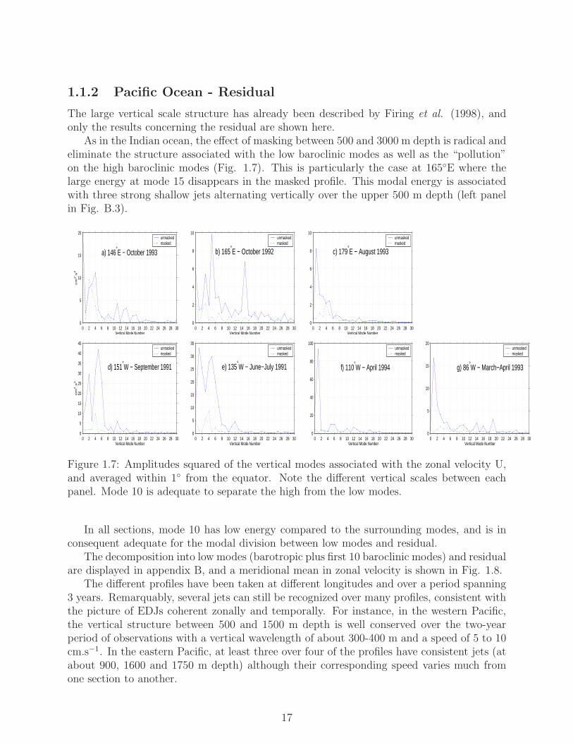
1.1.2 Pacific Ocean - Residual

The large vertical scale structure has already been described by Firing et al. (1998), andonly the results concerning the residual are shown here.

As in the Indian ocean, the effect of masking between 500 and 3000 m depth is radical andeliminate the structure associated with the low baroclinic modes as well as the “pollution”on the high baroclinic modes (Fig. 1.7). This is particularly the case at 165◦E where thelarge energy at mode 15 disappears in the masked profile. This modal energy is associatedwith three strong shallow jets alternating vertically over the upper 500 m depth (left panelin Fig. B.3).

cm

2.s

2


a) 146°E − October 1993

0 2 4 6 8 10 12 14 16 18 20 22 24 26 28 300

5

10

15

20unmaskedmasked


b) 165°E − October 1992

0 2 4 6 8 10 12 14 16 18 20 22 24 26 28 300

2

4

6

8

10unmaskedmasked


c) 179°E − August 1993

0 2 4 6 8 10 12 14 16 18 20 22 24 26 28 300

2

4

6

8

10unmaskedmasked

cm

2.s

2


d) 151°W − September 1991

0 2 4 6 8 10 12 14 16 18 20 22 24 26 28 300

5

10

15

20

25

30

35

40

45unmaskedmasked


e) 135°W − June−July 1991

0 2 4 6 8 10 12 14 16 18 20 22 24 26 28 300

5

10

15

20

25

30

35unmaskedmasked


f) 110°W − April 1994

0 2 4 6 8 10 12 14 16 18 20 22 24 26 28 300

20

40

60

80

100unmaskedmasked


g) 86°W − March−April 1993

0 2 4 6 8 10 12 14 16 18 20 22 24 26 28 300

5

10

15

20unmaskedmasked

Figure 1.7: Amplitudes squared of the vertical modes associated with the zonal velocity U,and averaged within 1◦ from the equator. Note the different vertical scales between eachpanel. Mode 10 is adequate to separate the high from the low modes.

In all sections, mode 10 has low energy compared to the surrounding modes, and is inconsequent adequate for the modal division between low modes and residual.

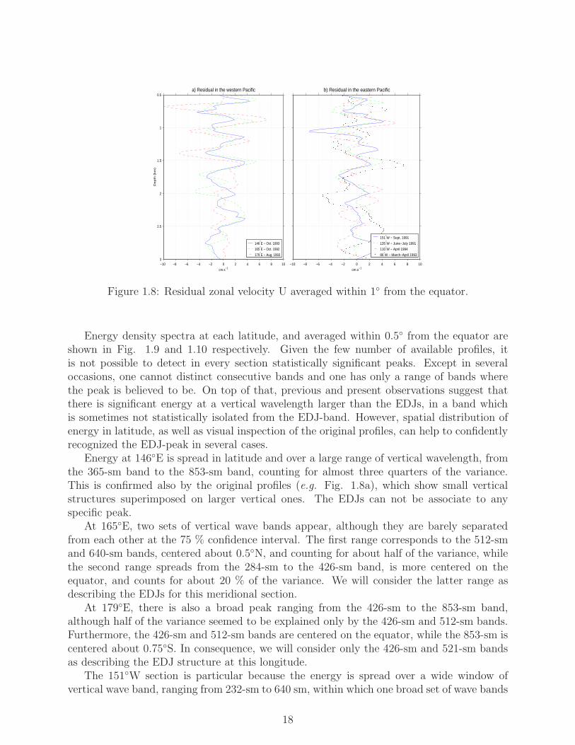
The decomposition into low modes (barotropic plus first 10 baroclinic modes) and residualare displayed in appendix B, and a meridional mean in zonal velocity is shown in Fig. 1.8.

The different profiles have been taken at different longitudes and over a period spanning3 years. Remarquably, several jets can still be recognized over many profiles, consistent withthe picture of EDJs coherent zonally and temporally. For instance, in the western Pacific,the vertical structure between 500 and 1500 m depth is well conserved over the two-yearperiod of observations with a vertical wavelength of about 300-400 m and a speed of 5 to 10cm.s−1. In the eastern Pacific, at least three over four of the profiles have consistent jets (atabout 900, 1600 and 1750 m depth) although their corresponding speed varies much fromone section to another.

17

a) Residual in the western Pacific

De

pth

(km

)

cm.s−1−10 −8 −6 −4 −2 0 2 4 6 8 103

2.5

2

1.5

1

0.5

146°E − Oct. 1993

165°E − Oct. 1992

179°E − Aug. 1993

b) Residual in the eastern Pacific

cm.s−1−10 −8 −6 −4 −2 0 2 4 6 8 10

151°W − Sept. 1991

135°W − June−July 1991

110°W − April 1994

86°W − March−April 1993

Figure 1.8: Residual zonal velocity U averaged within 1◦ from the equator.

Energy density spectra at each latitude, and averaged within 0.5◦ from the equator areshown in Fig. 1.9 and 1.10 respectively. Given the few number of available profiles, itis not possible to detect in every section statistically significant peaks. Except in severaloccasions, one cannot distinct consecutive bands and one has only a range of bands wherethe peak is believed to be. On top of that, previous and present observations suggest thatthere is significant energy at a vertical wavelength larger than the EDJs, in a band whichis sometimes not statistically isolated from the EDJ-band. However, spatial distribution ofenergy in latitude, as well as visual inspection of the original profiles, can help to confidentlyrecognized the EDJ-peak in several cases.

Energy at 146◦E is spread in latitude and over a large range of vertical wavelength, fromthe 365-sm band to the 853-sm band, counting for almost three quarters of the variance.This is confirmed also by the original profiles (e.g. Fig. 1.8a), which show small verticalstructures superimposed on larger vertical ones. The EDJs can not be associate to anyspecific peak.

At 165◦E, two sets of vertical wave bands appear, although they are barely separatedfrom each other at the 75 % confidence interval. The first range corresponds to the 512-smand 640-sm bands, centered about 0.5◦N, and counting for about half of the variance, whilethe second range spreads from the 284-sm to the 426-sm band, is more centered on theequator, and counts for about 20 % of the variance. We will consider the latter range asdescribing the EDJs for this meridional section.

At 179◦E, there is also a broad peak ranging from the 426-sm to the 853-sm band,although half of the variance seemed to be explained only by the 426-sm and 512-sm bands.Furthermore, the 426-sm and 512-sm bands are centered on the equator, while the 853-sm iscentered about 0.75◦S. In consequence, we will consider only the 426-sm and 521-sm bandsas describing the EDJ structure at this longitude.

The 151◦W section is particular because the energy is spread over a wide window ofvertical wave band, ranging from 232-sm to 640 sm, within which one broad set of wave bands

18

4−5

9−10

13−14

18−19

22−23

27−28

31−32

36−37

40−41

45−46

49−50

54−55

59−60

63−64

Str

etc

he

d V

ert

ica

l W

ave

len

gth

(sm

)

a) 146°E − October 1993

3°S 2°S 1°S 0° 1°N 2°N 3°N2560

1280

853

640

512

426

365

320

284

256

232

213

196

182

4−5

9−10

13−14

18−19

22−23

27−28

31−32

36−37

40−41

45−46

49−50

54−55

59−60

63−64

b) 165°E − October 1992

3°S 2°S 1°S 0° 1°N 2°N 3°N2560

1280

853

640

512

426

365

320

284

256

232

213

196

182

Ve

rtic

al M

od

e N

um

be

r

4−5

9−10

13−14

18−19

22−23

27−28

31−32

36−37

40−41

45−46

49−50

54−55

59−60

63−64

c) 179°E − August 1993

3°S 2°S 1°S 0° 1°N 2°N 3°N2560

1280

853

640

512

426

365

320

284

256

232

213

196

182

Energ

y Den

sity S

pectr

um (c

m2 .s−2)

104

105

106

107

108

4−5

9−10

13−14

18−19

22−23

27−28

31−32

36−37

40−41

45−46

49−50

54−55

59−60

63−64

Str

etc

he

d V

ert

ica

l W

ave

len

gth

(sm

)


3°S 2°S 1°S 0° 1°N 2°N 3°N2560

1280

853

640

512

426

365

320

284

256

232

213

196

182

4−5

9−10

13−14

18−19

22−23

27−28

31−32

36−37

40−41

45−46

49−50

54−55

59−60

63−64


3°S 2°S 1°S 0° 1°N 2°N 3°N2560

1280

853

640

512

426

365

320

284

256

232

213

196

182

4−5

9−10

13−14

18−19

22−23

27−28

31−32

36−37

40−41

45−46

49−50

54−55

59−60

63−64

f) 110°W − April 1994

3°S 2°S 1°S 0° 1°N 2°N 3°N2560

1280

853

640

512

426

365

320

284

256

232

213

196

182

Ve

rtic

al M

od

e N

um

be

r

4−5

9−10

13−14

18−19

22−23

27−28

31−32

36−37

40−41

45−46

49−50

54−55

59−60

63−64

g) 85°W − March−April 1993

3°S 2°S 1°S 0° 1°N 2°N 3°N2560

1280

853

640

512

426

365

320

284

256

232

213

196

182

Figure 1.9: As in Fig. 1.5 but for the Pacific Ocean sections.


4−5 9−10 13−14 18−19 22−23 27−28 31−32 36−37 40−41 45−46 49−50 54−55 59−60 63−64

10

8 ×

(scm

/s)2

/cp

sm

a) 146°E − October 1993

20 %19 %

15 %

2560 1280 853 640 512 426 365 320 284 256 232 213 196 182 0

0.2

0.4

0.6

0.8

1


4−5 9−10 13−14 18−19 22−23 27−28 31−32 36−37 40−41 45−46 49−50 54−55 59−60 63−64

b) 165°E − October 199227 %

22 %

11 %8 %

2560 1280 853 640 512 426 365 320 284 256 232 213 196 182 0

0.2

0.4

0.6

0.8

1


4−5 9−10 13−14 18−19 22−23 27−28 31−32 36−37 40−41 45−46 49−50 54−55 59−60 63−64

c) 179°E − August 199327 %

25 %

2560 1280 853 640 512 426 365 320 284 256 232 213 196 182 0

0.2

0.4

0.6

0.8

1

4−5 9−10 13−14 18−19 22−23 27−28 31−32 36−37 40−41 45−46 49−50 54−55 59−60 63−64

10

8 ×

(scm

/s)2

/cp

sm


17 %20 %

15 %

10 %

Stretched Vertical Wavelength (sm)2560 1280 853 640 512 426 365 320 284 256 232 213 196 182 0

0.2

0.4

0.6

0.8

1

4−5 9−10 13−14 18−19 22−23 27−28 31−32 36−37 40−41 45−46 49−50 54−55 59−60 63−64


Stretched Vertical Wavelength (sm)

17 %

42 %

2560 1280 853 640 512 426 365 320 284 256 232 213 196 182 0

0.2

0.4

0.6

0.8

1

4−5 9−10 13−14 18−19 22−23 27−28 31−32 36−37 40−41 45−46 49−50 54−55 59−60 63−64

f) 110°W − April 1994

25 %

19 %


0.2

0.4

0.6

0.8

1

4−5 9−10 13−14 18−19 22−23 27−28 31−32 36−37 40−41 45−46 49−50 54−55 59−60 63−64

g) 85 °W − March−April 1993

37 %


0.2

0.4

0.6

0.8

1

9 %

Figure 1.10: Energy density spectrum averaged within 0.5◦ from the equator. The grey areashows the 75 % confidence interval, and the numbers describe the percentage of varianceexplained by some of the peaks. Arrows show statistically significant peaks within a singleband, while horizontal bars show consecutive bands which can not be distinct statisticallybut have nonetheless significant energy.

19

and two statistically significant peaks and can be distinguished. The broad set contains the365-sm, 426-sm, 512-sm and 640-sm bands and explains about half of the variance. Thetwo significative peaks are located at the 284-sm and 232-sm bands, explaining 15 and 10 %respectively of the variance, and are trapped between 1◦S and 0.5◦N. This is consistent withthe original profiles (e.g. Fig. 1.8b) which show a quite irregular structure in the vertical.Thus, no specific wave band will be associated here to the EDJs.

The 135◦W section is the most satisfying statistically speaking. There are two statisticallysignificant peaks in the 853-sm and 426-sm bands, explaining 17 and 42 % of the variancerespectively. The 426-sm peak is the one considered as describing the EDJs due to itsequatorial trapping.

At 110◦W, energy is contained in a broad window ranging from the 365-sm to the 640-sm bands. Within this range, one can isolate the 365-sm and 426-sm consecutive bandsfrom the 512-sm and 640-sm consecutive bands, not based on statistics, but on their spatialdistribution, the former one seeming to be more equatorially trapped than the latter one.Thus, we will consider the 365-sm and 426-sm bands are the ones describing the EDJs atthis longitude.

Finally, the easternmost section at 85 ◦W has a strong peak in the 640-sm and 853-smbands, the 640-sm band explaining 37 % of the variance by itself. This is confirmed by thelarge vertical scale seen in the original profiles (e.g. Fig. 1.8b). There is also a smallerbut statistically significant peak in the 284-sm band, explaining about 10 % of the variance.Because we do not think that the first peak is typical of the EDJs, we will not associate hereany peak to the EDJs.

20

Appendix A

Plate Indian Ocean

21

0.25

0.2

0.1

Dep

th (

km)

U

3°S 1.5°S 0° 1.5°N 3°N4.5

4

3.5

3

2.5

2

1.5

1

0.5

Low mode U

3°S 1.5°S 0° 1.5°N 3°N

Residual U

U at 57°E − March and April 1995

3°S 1.5°S 0° 1.5°N 3°N

Figure A.1: Zonal velocity U along the line I7N at 57◦E, during March and April 1995. Theleft panels show the full velocity, the middle panels show the low modes (barotropic plus first9 baroclinic modes), and the right panel shows the residual. The top panels show the top250 m. This decomposition has been done without masking the upper 5000 and lower 3000m depth. Especially, the top 250 m of the residual is polluted by mathematical artifactsfrom the decomposition, and is not shown. Contour intervals are each 5 cm.s−1. Shadedareas indicate negative values. Tick marks on top axis indicate the latitudes of observations.

22

0.25

0.2

0.1

Dep

th (

km)

V

3°S 1.5°S 0° 1.5°N 3°N4.5

4

3.5

3

2.5

2

1.5

1

0.5

Low mode V

3°S 1.5°S 0° 1.5°N 3°N

Residual V

V at 57°E − March and April 1995

3°S 1.5°S 0° 1.5°N 3°N

Figure A.2: Same as Fig. A.1 but for the meridional velocity V along the line I7N at 57◦E,during March and April 1995.

23

0.25

0.2

0.1

Dep

th (

km)

U

3°S 1.5°S 0° 1.5°N 3°N4.5

4

3.5

3

2.5

2

1.5

1

0.5

Low mode U

3°S 1.5°S 0° 1.5°N 3°N

Residual U

U at 57°E − June 1995

3°S 1.5°S 0° 1.5°N 3°N

Figure A.3: Same as Fig. A.1 but for the zonal velocity U along the line I7N at 57◦E, duringJune 1995.

24

0.25

0.2

0.1

Dep

th (

km)

V

3°S 1.5°S 0° 1.5°N 3°N4.5

4

3.5

3

2.5

2

1.5

1

0.5

Low mode V

3°S 1.5°S 0° 1.5°N 3°N

Residual V

V at 57°E − June 1995

3°S 1.5°S 0° 1.5°N 3°N

Figure A.4: Same as Fig. A.1 but for the meridional velocity V along the line I7N at 57◦E,during June 1995.

25

0.25

0.2

0.1

Dep

th (

km)

U

3°S 1.5°S 0° 1.5°N 3°N4.5

4

3.5

3

2.5

2

1.5

1

0.5

Low mode U

3°S 1.5°S 0° 1.5°N 3°N

Residual U

U at 57°E − July and August 1995

3°S 1.5°S 0° 1.5°N 3°N

Figure A.5: Same as Fig. A.1 but for the zonal velocity U along the line I7N at 57◦E, duringJuly and August 1995.

26

0.25

0.2

0.1

Dep

th (

km)

V

3°S 1.5°S 0° 1.5°N 3°N4.5

4

3.5

3

2.5

2

1.5

1

0.5

Low mode V

3°S 1.5°S 0° 1.5°N 3°N

Residual V

V at 57°E − July and August 1995

3°S 1.5°S 0° 1.5°N 3°N

Figure A.6: Same as Fig. A.1 but for the meridional velocity V along the line I7N at 57◦E,during July and August 1995.

27

0.25

0.2

0.1

Dep

th (

km)

U

3°S 1.5°S 0° 1.5°N 3°N4.5

4

3.5

3

2.5

2

1.5

1

0.5

Low mode U

3°S 1.5°S 0° 1.5°N 3°N

Residual U

U at 80°E − March and April 1995

3°S 1.5°S 0° 1.5°N 3°N

Figure A.7: Same as Fig. A.1 but for the zonal velocity U along the line I8N at 80◦E, duringMarch and April 1995.

28

0.25

0.2

0.1

Dep

th (

km)

V

3°S 1.5°S 0° 1.5°N 3°N4.5

4

3.5

3

2.5

2

1.5

1

0.5

Low mode V

3°S 1.5°S 0° 1.5°N 3°N

Residual V

V at 80°E − March and April 1995

3°S 1.5°S 0° 1.5°N 3°N

Figure A.8: Same as Fig. A.1 but for the meridional velocity V along the line I8N at 80◦E,during March and April 1995.

29

0.25

0.2

0.1

Dep

th (

km)

U

3°S 1.5°S 0° 1.5°N 3°N4.5

4

3.5

3

2.5

2

1.5

1

0.5

Low mode U

3°S 1.5°S 0° 1.5°N 3°N

Residual U

U at 80°E − September and October 1995

3°S 1.5°S 0° 1.5°N 3°N

Figure A.9: Same as Fig. A.1 but for the zonal velocity U along the line I8N at 80◦E, duringSeptember and October 1995. No observation has been done below 3000 m depth.

30

0.25

0.2

0.1

Dep

th (

km)

V

3°S 1.5°S 0° 1.5°N 3°N4.5

4

3.5

3

2.5

2

1.5

1

0.5

Low mode V

3°S 1.5°S 0° 1.5°N 3°N

Residual V

V at 80°E − September and October 1995

3°S 1.5°S 0° 1.5°N 3°N

Figure A.10: Same as Fig. A.1 but for the meridional velocity V along the line I8N at 80◦E,during September and October 1995. No observation has been done below 3000 m depth.

31

0.25

0.2

0.1

Dep

th (

km)

U

3°S 1.5°S 0° 1.5°N 3°N4.5

4

3.5

3

2.5

2

1.5

1

0.5

Low mode U

3°S 1.5°S 0° 1.5°N 3°N

Residual U

U at 93°E − January and March 1995

3°S 1.5°S 0° 1.5°N 3°N

Figure A.11: Same as Fig. A.1 but for the zonal velocity U along the line I9N at 93◦E,during January and April 1995.

32

0.25

0.2

0.1

Dep

th (

km)

V

3°S 1.5°S 0° 1.5°N 3°N4.5

4

3.5

3

2.5

2

1.5

1

0.5

Low mode V

3°S 1.5°S 0° 1.5°N 3°N

Residual V

V at 93°E − January and March 1995

3°S 1.5°S 0° 1.5°N 3°N

Figure A.12: Same as Fig. A.1 but for the meridional velocity V along the line I9N at 93◦E,during January and April 1995.

33

Appendix B

Plate Pacific Ocean

34

0.25

0.2

0.1

Dep

th (

km)

U

3°S 1.5°S 0° 1.5°N 3°N4.5

4

3.5

3

2.5

2

1.5

1

0.5

0.25

0.2

0.1

Low Mode U

3°S 1.5°S 0° 1.5°N 3°N

Residual U

U at 146°E − October and November 1993

3°S 1.5°S 0° 1.5°N 3°N

Figure B.1: Zonal velocity U along the line P10 at 146◦E, during October and November1993. The left panels show the full velocity, the middle panels show the low modes (barotropicplus first 11 baroclinic modes), and the right panel shows the residual. The top panels showthe top 250 m. This decomposition has been done without masking the upper 5000 and lower3000 m depth. Especially, the top 250 m of the residual is polluted by mathematical artifactsfrom the decomposition, and is not shown. Contour intervals are each 5 cm.s−1. Shadedareas indicate negative values. Tick marks on top axis indicate the latitudes of observations.

35

0.25

0.2

0.1

Dep

th (

km)

V

3°S 1.5°S 0° 1.5°N 3°N4.5

4

3.5

3

2.5

2

1.5

1

0.5

0.25

0.2

0.1

Low Mode V

3°S 1.5°S 0° 1.5°N 3°N

Residual V

V at 146°E − October and November 1993

3°S 1.5°S 0° 1.5°N 3°N

Figure B.2: Same as Fig. B.1 but for the meridional velocity V along the line P10 at 146◦E,during October and November 1993.

36

0.25

0.2

0.1

Dep

th (

km)

U

3°S 1.5°S 0° 1.5°N 3°N4.5

4

3.5

3

2.5

2

1.5

1

0.5

0.25

0.2

0.1

Low Mode U

3°S 1.5°S 0° 1.5°N 3°N

Residual U

U at 165°E − September and October 1992

3°S 1.5°S 0° 1.5°N 3°N

Figure B.3: Same as Fig. B.1 but for the zonal velocity U along the line P13 at 165◦E,during September and October 1992.

37

0.25

0.2

0.1

Dep

th (

km)

V

3°S 1.5°S 0° 1.5°N 3°N4.5

4

3.5

3

2.5

2

1.5

1

0.5

0.25

0.2

0.1

Low Mode V

3°S 1.5°S 0° 1.5°N 3°N

Residual V


3°S 1.5°S 0° 1.5°N 3°N

Figure B.4: Same as Fig. B.1 but for the meridional velocity V along the line P13 at 165◦E,during September and October 1992.

38

0.25

0.2

0.1

Dep

th (

km)

U

3°S 1.5°S 0° 1.5°N 3°N4.5

4

3.5

3

2.5

2

1.5

1

0.5

0.25

0.2

0.1

Low Mode U

3°S 1.5°S 0° 1.5°N 3°N

Residual U

U at 179°E − August 1993

3°S 1.5°S 0° 1.5°N 3°N

Figure B.5: Same as Fig. B.1 but for the zonal velocity U along the line P14 at 179◦E,during August 1993.

39

0.25

0.2

0.1

Dep

th (

km)

V

3°S 1.5°S 0° 1.5°N 3°N4.5

4

3.5

3

2.5

2

1.5

1

0.5

0.25

0.2

0.1

Low Mode V

3°S 1.5°S 0° 1.5°N 3°N

Residual V


3°S 1.5°S 0° 1.5°N 3°N

Figure B.6: Same as Fig. B.1 but for the meridional velocity V along the line P14 at 179◦E,during August 1993.

40

0.25

0.2

0.1

Dep

th (

km)

U

3°S 1.5°S 0° 1.5°N 3°N4.5

4

3.5

3

2.5

2

1.5

1

0.5

0.25

0.2

0.1

Low Mode U

3°S 1.5°S 0° 1.5°N 3°N

Residual U

U at 151°W − September and October 1991

3°S 1.5°S 0° 1.5°N 3°N

Figure B.7: Same as Fig. B.1 but for the zonal velocity U along the line P16 at 151◦W,during September and October 1991.

41

0.25

0.2

0.1

Dep

th (

km)

V

3°S 1.5°S 0° 1.5°N 3°N4.5

4

3.5

3

2.5

2

1.5

1

0.5

0.25

0.2

0.1

Low Mode V

3°S 1.5°S 0° 1.5°N 3°N

Residual V

V at 151°W − September and October 1991

3°S 1.5°S 0° 1.5°N 3°N

Figure B.8: Same as Fig. B.1 but for the meridional velocity V along the line P16 at 151◦W,during September and October 1991.

42

0.25

0.2

0.1

Dep

th (

km)

U

3°S 1.5°S 0° 1.5°N 3°N4.5

4

3.5

3

2.5

2

1.5

1

0.5

0.25

0.2

0.1

Low Mode U

3°S 1.5°S 0° 1.5°N 3°N

Residual U

U at 135°W − May and July 1991

3°S 1.5°S 0° 1.5°N 3°N

Figure B.9: Same as Fig. B.1 but for the zonal velocity U along the line P17 at 135◦W,during May and July 1991.

43

0.25

0.2

0.1

Dep

th (

km)

V

3°S 1.5°S 0° 1.5°N 3°N4.5

4

3.5

3

2.5

2

1.5

1

0.5

0.25

0.2

0.1

Low Mode V

3°S 1.5°S 0° 1.5°N 3°N

Residual V

V at 135°W − May and July 1991

3°S 1.5°S 0° 1.5°N 3°N

Figure B.10: Same as Fig. B.1 but for the meridional velocity V along the line P17 at135◦W, during May and July 1991.

44

0.25

0.2

0.1

Dep

th (

km)

U

3°S 1.5°S 0° 1.5°N 3°N4.5

4

3.5

3

2.5

2

1.5

1

0.5

0.25

0.2

0.1

Low Mode U

3°S 1.5°S 0° 1.5°N 3°N

Residual U

U at 110°W − March and April 1994

3°S 1.5°S 0° 1.5°N 3°N

Figure B.11: Same as Fig. B.1 but for the zonal velocity U along the line P18 at 110◦W,during March and April 1994.

45

0.25

0.2

0.1

Dep

th (

km)

V

3°S 1.5°S 0° 1.5°N 3°N4.5

4

3.5

3

2.5

2

1.5

1

0.5

0.25

0.2

0.1

Low Mode V

3°S 1.5°S 0° 1.5°N 3°N

Residual V

V at 110°W − March and April 1994

3°S 1.5°S 0° 1.5°N 3°N

Figure B.12: Same as Fig. B.1 but for the meridional velocity V along the line P18 at110◦W, during March and April 1994.

46

0.25

0.2

0.1

Dep

th (

km)

U

3°S 1.5°S 0° 1.5°N 3°N4.5

4

3.5

3

2.5

2

1.5

1

0.5

0.25

0.2

0.1

Low Mode U

3°S 1.5°S 0° 1.5°N 3°N

Residual U

U at 86°W − February to April 1993

3°S 1.5°S 0° 1.5°N 3°N

Figure B.13: Same as Fig. B.1 but for the zonal velocity U along the line P19 at 86◦W,during February to April 1993. No observations have been done below 3000 m depth.

47

0.25

0.2

0.1

Dep

th (

km)

V

3°S 1.5°S 0° 1.5°N 3°N4.5

4

3.5

3

2.5

2

1.5

1

0.5

0.25

0.2

0.1

Low Mode V

3°S 1.5°S 0° 1.5°N 3°N

Residual V

V at 86°W − February to April 1993

3°S 1.5°S 0° 1.5°N 3°N

Figure B.14: Same as Fig. B.1 but for the meridional velocity V along the line P19 at 86◦W,during February to April 1993. No observations have been done below 3000 m depth.

48

the equatorial subthermocline … equatorial subthermocline circulation in observations ... ocean...

Documents