NBER WORKING PAPER SERIES

THE EQUALITY MULTIPLIER

Erling BarthKarl O. Moene

Working Paper 15076http://www.nber.org/papers/w15076

NATIONAL BUREAU OF ECONOMIC RESEARCH1050 Massachusetts Avenue

Cambridge, MA 02138June 2009

This work is part of a larger research project at ESOP, the Frisch center and the Institute for SocialResearch. We are grateful for comments by Jon Fiva, Jeff Frieden, Steinar Holden, Torben Iversen,Jo Thori Lind, Atle Seierstad, Fredrik Willumsen. Research Grants from the Research Council of Norway,grantnumber 168 285/S20, are gratefully acknowledged. Erling Barth thanks the Labor and Worklife Programat Harvard University and the National Bureau of Economic Research for their generosity and hospitalityduring his work with this paper. The views expressed herein are those of the author(s) and do not necessarilyreflect the views of the National Bureau of Economic Research.

NBER working papers are circulated for discussion and comment purposes. They have not been peer-reviewed or been subject to the review by the NBER Board of Directors that accompanies officialNBER publications.

© 2009 by Erling Barth and Karl O. Moene. All rights reserved. Short sections of text, not to exceedtwo paragraphs, may be quoted without explicit permission provided that full credit, including © notice,is given to the source.

The Equality MultiplierErling Barth and Karl O. MoeneNBER Working Paper No. 15076June 2009JEL No. H53,J31,P16

ABSTRACT

Equality can multiply due to the complementarity between wage determination and welfare spending.A more equal wage distribution fuels welfare generosity via political competition. A more generouswelfare state fuels wage equality further via its support to weak groups in the labor market. Togetherthe two effects generate a cumulative process that adds up to an important social multiplier. We focuson a political economic equilibrium which incorporates this mutual dependence between wage settingand welfare spending. It explains how almost equally rich countries differ in economic and social equalityamong their citizens and why countries cluster around different worlds of welfare capitalism---theScandinavian model, the Anglo-Saxon model and the Continental model. Using data on 18 OECDcountries over the period 1976-2002 we test the main predictions of the model and identify a sizeablemagnitude of the equality multiplier. We obtain additional support for the cumulative complementaritybetween social spending and wage equality by applying another data set for the US over the period1945-2001.

Erling BarthInstitute for Social ResearchPb 3233 Elisenberg0208 OsloNorwayeba@samfunnsforskning.no

Karl O. MoeneDepartment of EconomicsUniversity of OsloPb 1095 Blindern0317 OsloNorwayk.o.moene@econ.uio.no

1 Introduction

With only half of the pre-tax wage inequality of the US, the Scandinavian countries of

Denmark, Norway and Sweden have twice as generous welfare spending as the US. This is

a stark illustration of a general pattern illustrated in Figure 1. The vertical axis measures

an index of the generosity of the welfare state and the horizontal axis measures the ratio

of the 9th decile to the 1st decile of gross hourly wage. The pattern is visible regardless

of what measures we use: Countries with smaller wage differentials tend to have more

generous welfare spending, and visa versa1.

This pattern is also visible within single countries over time. In the US, for instance,

public social transfers were established by president president F.D Roosevelt in the land-

mark Social Security Act of 1935. The first years after World War II social spending

increased considerably as percent of GDP. At the same time, wage inequality dropped to

the extent that Claudia Goldin and Robert Margo (1992) labeled this period the time

of the ”Great Compression”. During the era of president Ronald Reagan, there was a

period of considerable retrenchment in social spending. At the same time, wage inequality

surged to unprecedented levels. Figure 2 illustrates this pattern over time: Periods with

less growth in wage differentials tend to have higher growth in welfare generosity, and vise

versa.

Below we offer two separate mechanisms with distinct causal effects that together can

explain this general pattern. One mechanism, the equality magnifying effect, runs from

the wage distribution to the determination of welfare state policies: More wage equality

leads the majority of voters to support a more generous welfare state. This positive

association resembles what Peter Lindert (2004) calls the ’Robin Hood paradox’ in which

redistribution from the rich to the poor is least present where it is the most needed.2

The other mechanism, the wage equalizing effect, runs from welfare state policies to

wage determination: More generous welfare benefits lead to more wage equality as weak

groups in the labor market improve their relative bargaining position, allowing them

to command a higher pay. In this way improved welfare benefits compresses the wage

distribution from below.

Combining the two effects we have two mechanisms that are complementary. A more

equal wage distribution fuels welfare generosity and a more generous welfare state fuels

wage equality, stimulating further welfare generosity and further wage equality in a cu-

1In the appendix, we show that this pattern is robust to a host of different types of measures.2Lindert draws attention to a more general regularity than we do: ”Poverty policy within any one

polity or jurisdiction is supposed to aid the poor more, the lower the average income and the greater theincome inequality. Yet over time and space, the pattern is usually the opposite”. (Lindert 2004, p 15.)This equality-generosity puzzle runs counter to the most prominent theories of welfare spending such asthe seminal papers by Romer (1975), Roberts (1977), and Meltzer and Richard (1981) which all predictthat higher pre-tax inequality should be associated with a more generous welfare state.

1

Figure 1: Welfare Generosity and Wage Inequality across Countries

Australia

Austria

Belgium

Canada

Denmark

Finland

France

Germany

Ireland

Italy

Japan

Netherland

New Zealand

NorwaySweden

Switzerland

United KingdomUnited States

2025

3035

40G

ener

osity

Inde

x

2 2.5 3 3.5 4 4.5Wage Dispersion

Note: Wage dispersion is the ratio of the 9th decile to the 1st decile of gross hourly wage. Source: mainlyOECD, see data appendix. Overall Generosity Index is an index of welfare generosity developed by LyleScruggs, University of Connecticut, see data appendix. The figure shows average values in our data overthe time period 1976-2002. N=361

mulative process. This process can add up to a sizeable social multiplier.3 Our paper

provides a theoretical explanation of the mechanisms behind this equality multiplier and

an empirical assessment of its magnitude in OECD countries.

In order to do so we derive an equilibrium where the level of equality induces social

policies that again induce the level of equality. This is an example of Toqueville’s (1835)

observation that ”equality ...gives a certain direction to public spirit, a certain turn to

the laws, new maxims to those who govern, and particular habits to the governed”(p 3).

The political-economic equilibrium we derive is not converging across countries. On the

contrary, it is contingent on specific organizations and institutions.

We emphasize how certain policies and institutions fit together and strengthen each

other. Societal arrangements therefore tend to come in different clusters of social and

economic characteristics. One example is ”the three worlds of welfare capitalism”, distin-

3Glaeser, Sacerdote and Schenkman (2003) discuss social multipliers where individual behavior de-pends on aggregate behaviors. In our case the complementarity is between institutions of the labormarket and the welfare state.

2

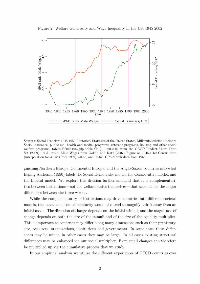
Figure 2: Welfare Generosity and Wage Inequality in the US. 1945-2002

05

1015

Soci

al T

rans

fers

/GD

P

33.

54

4.5

5d9

d1 ra

tio, M

ale

Wag

es

1945 1950 1955 1960 1965 1970 1975 1980 1985 1990 1995 2000year

d9d1 ratio, Male Wages Social Transfers/GDP

Sources: Social Transfers 1945-1959, Historical Statistics of the United States, Millennial edition (includesSocial insurance, public aid, health and medial programs, veterans programs, housing and other socialwelfare programs, tables Bf189-195/gdp table Ca1); 1960-2001 from the OECD Lindert-Allard DataSet (2009). d9d1 ratio, Male Wages from Goldin and Katz (2007) Figure 5: 1945-1960 Census data(interpolation for 45-48 (from 1939), 50-58, and 60-62. CPS-March data from 1963.

guishing Northern Europe, Continental Europe, and the Anglo-Saxon countries into what

Esping Andersen (1990) labels the Social Democratic model, the Conservative model, and

the Liberal model. We explore this division further and find that it is complementari-

ties between institutions—not the welfare states themselves—that account for the major

differences between the three worlds.

While the complementarity of institutions may drive countries into different societal

models, the exact same complementarity would also tend to magnify a drift away from an

initial mode. The direction of change depends on the initial stimuli, and the magnitude of

change depends on both the size of the stimuli and of the size of the equality multiplier.

This is important as countries may differ along many dimensions such as their prehistory,

size, resources, organizations, institutions and governments. In some cases these differ-

ences may be minor, in other cases they may be large. In all cases existing structural

differences may be enhanced via our social multiplier. Even small changes can therefore

be multiplied up via the cumulative process that we study.

In our empirical analysis we utilize the different experiences of OECD countries over

3

26 years from 1976 to 2002 in order to identify both the equality magnifying effect as

well as the wage equalizing effect, and thereby to provide an estimate of the size of the

equality multiplier. We also offer some supporting evidence by taking a closer look at the

development of welfare generosity and wage inequality in the Post-World-War-II United

States. The US is a particularly interesting example since it represents an extreme case

with high wage dispersion and low welfare generosity, but also because there seems to be

high expectations of changes arising from the new presidency of Barak Obama; changes

that may affect both inequality and welfare generosity in the US.

Our focus extends the welfare state literature by incorporating one important aspect

of the mutual dependence between markets and politics. We add the reverse linkage to the

analysis of how wage equality fuels the political demand for social insurance against loss of

income (see Iversen and Soskice, 2001, and Moene and Wallerstein, 2001). More generally,

our paper contributes to the discussion of why welfare spending is so much higher in some

countries than in others and why not all countries have an European style welfare state

(see Alesina and Glaeser 2001, 2004 for a broad political economic approach, Lindert,

2004, for a comprehensive historical overview, and Cameroon 1978 and Katzenstein 1985

for the role of openness and country size)).

Our analysis also adds to the ongoing discussion of why seemingly similar countries

sustain widely differing wage structures, in particular on the relative impact of market

forces versus institutions in explaining cross country differences in the wage structure

(see eg. Devroye and Freeman (2001), Leuven et al. (2004), Blau and Kahn (1996),

Acemoglu (2003)), and Scheve and Stasavage (2008); and in explaining the development

of wage inequality within countries over time (see eg. Katz and Murphy (1992), Card and

DiNardo (2002), Autor et al. (2008), and Goldin and Katz (2006) for studies with focus

on the US experience).

Section 2 gives our basic argument and presents the equality multiplier. Section 3

explains the equality magnifying effect and section 4 explains the wage equalizing effect.

The empirical analysis is provided in sections 5 to 7. Section 8 concludes.

2 The basic argument

For each country j we combine two distinct mechanisms that can be associated with two

downward sloping curves between wage inequality Ij and welfare generosity Gj.

2.1 The equality magnifying curve

The equality magnifying curve captures how equality in the distribution of pre-tax wages

raises the generosity of the welfare state. It relates to the political competition over voters’

support where the interests of voters are shaped by the pre-tax distribution of wages.

4

In short the mechanism can be written as

ln(Gj) = Aj − aI ln(Ij) where Aj = A(zj) (1)

Here welfare generosity in country j is supposed to depend on country characteristics

Aj where zj is a vector including such things as the political orientation of the winning

party, the income level of the country, and indicators that pick up the economic risks that

voters are exposed to such as economic openness. Our main interest is related to aI > 0

capturing the equality magnifying effect.

As we discuss further in section 3 a more compressed wage distribution, for a given

mean, makes the majority of workers richer which in turn raises the political support for

a generous welfare spending on commodities and services that are normal goods for the

households. Deriving this equality magnifying effect we emphasize that protection against

risks has been more universally sought and has been more important for the expansion of

the welfare state, than pure redistribution of resources (Baldwin 1990, Barr 1992). Welfare

policies that, in addition to providing a more fair distribution, cover social demands for

which the market fails to provide, are much more likely to be both legitimate and popular.

Building on Moene and Wallerstein (2001, 2003) we focus on welfare spending as social

insurance against loss of income due to sickness, unemployment, and old age. It matters

which party wins the election, but all parties run on a program that is already adjusted

to the wage distribution.

2.2 The wage equalizing curve

The wage equalizing curve captures how the generosity of the welfare state Gj strengthens

weak group in the labor market. In short the mechanism is written as

ln(Ij) = Bj − agln(Gj) where Bj = B(yj) (2)

Here wage inequality in country j is supposed to depend on country characteristics Bj

where yj is a vector including such things as indicators of the wage setting system, union

density, and the level of income in the country (some of which may be shared with the

vector z, of course). Our main interest is related to ag > 0 capturing the wage equalizing

effect.

As we discuss further in section 4 welfare benefits compresses the pre tax wage distri-

bution from below. Deriving this wage equalizing effect, we focus on a simple bargaining

framework where welfare benefits raises the fall back position of particularly vulnerable

groups. They are therefore able to command a higher pay and to improve their relative

wage. The bargaining framework allows for both decentralized and more coordinated

wage setting.

5

2.3 Equilibrium and the equality multiplier

Combining the two curves we obtain a political economic equilibrium which incorporates

the mutual dependence between wage setting and welfare spending. While welfare spend-

ing depends on wage inequality, it also feeds back to the determination of the level of

wage inequality. The equilibrium outcome is the wage inequality and the level of welfare

spending that are consistent taking the mutual feed-backs into account. It can be reached

after a cumulative sequence of wage settlements and welfare state adjustments.

The equilibrium levels of welfare generosity and wage distribution are

ln(Gj) = m[Aj − aIBj] and ln(Ij) = m[Bj − agAj] (3)

where m is the multiplier given by

m =1

1− aIag(4)

which is greater than one whenever the system is stable, i.e. whenever aI < 1/ag.

The equilibrium levels shift with changing circumstances and there is an equality mul-

tiplier (or inequality multiplier, depending on the stimuli) m between wage setting and

welfare spending. The multiplier summarizes the feed back mechanisms between the

equality magnifying effect and the wage equalizing effect. The effects of shifts in Aj (for

instance caused by a change of the political color of government) or in Bj (for instance

caused by a change in the level of wage coordination) are then magnified by m > 1. A

rise in Aj, for instance,would lead to a total effect of∆GjGj

= m∆Aj on welfare generosity

and to a total effect on wage inequality of∆IjIj

= mag∆Aj.

3 Deriving the Equality Magnifying Effect

In this section we derive and characterize the relationship ln(G) = A− aI ln(I), focussing

on how the political demand for protection against risk can be understood as a main

mechanism behind the emergence of modern welfare states. We consider a society with

a continuum of voters normalized to 1. They have jobs or occupations with different

productivity and risks of income loss. The productivity p has continuous distribution

with E(p) = p, (throughout we use the expectation operator to indicate averages). In the

exposition the distribution of p is given, but how earnings relates to productivity vary

with wage determination systems as discussed in Section 4. There we derive how earnings

are an increasing function of the productivity p of the position. We write it w(p), where

w′(p) ≥ 0. b

6

3.1 Welfare generosity: Voters’ preferences

The social chance that a person in position p will be on welfare benefits is e(p). It reflects

a combination of the risks of loosing one’s income and the willingness to utilize welfare

state arrangements. Richer workers tend to be less inclined to use the welfare state partly

because they have a lower chance of job loss of a certain duration (they more easily get

a new one) and partly because they tend to rely more on self insurance. We express this

as e′(p) ≤ 0.

As above we denote by G the generosity of the welfare system. In most welfare systems

social insurance is offered on better terms for low wage earners than for high wage earners.

We incorporate this by assuming that each worker who loses his income obtains welfare

benefits equal to G. This is of course a grave simplification, but one that can easily be

modified.4

The welfare benefits are financed by a constant marginal tax t on total income (wages

plus profits), E[(1 − e(p))p], which we think of as representing total income per capita.

To simplify we abstract from deadweight losses. The balanced budget equation is then

t = γG with γ =E[e(p)]

E[(1− e(p))p](5)

The cost of welfare generosity is γ, measuring the impact on the tax rate of an increase

in the generosity level of welfare spending. Thus the cost of welfare generosity is low

whenever total income is high and the fraction citizens in need of support is low. Note

that 1/γ expresses total income per capita relative to the average fraction of citizens

without their ordinary pay.

The narrow self interests of a each citizen is expressed by an utility function with a

constant relative risk aversion µ over consumption c

U (c) ≡ 1

1− µc1−µ with µ > 1

Since the individual risk of income loss must be considered a serious threat to the liv-

4In general, some benefits are proportional to present earnings or past contributions; others are not.We could have incorporated this by a given parameter θ ∈ (0, 1] reflecting the composition of welfarespending and the extent to which the poor are offered social insurance on better terms than the rich:

G(p) =(θ + (1− θ) w(p)

Ew(p)

)G

The benefits G (the benefit level to workers with the average wage) of the social insurance scheme aredistributed with a fixed component common to all and a variable component that depends on past andpresent contributions. The fixed component is θG which defines the floor of welfare benefits to people with-out income. The variable component is proportional to income relative to the mean G (1− θ)w(p)/Ew(p),implying that here G(p) is the welfare benefits to a worker in position p in the event of income loss. Thehigher is θ the more redistributive is the terms of the social insurance scheme. In the presentation weapply the simplifying assumption that θ = 1.

7

ing conditions of a typical voter, we limit the discussion to cases where citizens have a

relatively high degree of risk aversion µ > 1

Voters have political interests that reflect their social identification with people who

have lost their income. The social preferences of voters are expressed as modified expected

utility, where the weight on being without ordinary income is enhanced by a parameter

h ≥ 1 capturing social care. Inserting c(p) = (1− t)w(p) and t = γg the social preferences

of a worker in position p are

v (g; p) = (1− e(p))U ((1− γG)w(p)) + e(p)hU (G) (6)

When h = 1, we have the narrow self-interested case of standard expected utility; when

h > 1 the probability e(p) is enhanced further. The extra weight e(p)(h−1) captures social

identification: A voter in position p is assumed to have a stronger social identification

with people who have lost their income, the more likely it is that he may end up on welfare

himself.

We find his most preferred generosity of the welfare state—his ideal policy—from the

first order condition ∂v(G; p)/∂G = 0, which after some rearranging can be written as

G(p) =(w(p))

µ−1µ(

γ(1−e(p))e(p)h

) 1µ

+ γ (w(p))µ−1µ

(7)

The most preferred welfare generosity G(p) by a voter in position p depends positively

on (i) his gross income w(p), (ii) his odds e/(1− e) of loosing the income, (iii) his social

care h, and (iv) society’s income per capita 1/γ relative to the average fraction of people

without an income.

Opinion surveys in OECD countries show that high-paid wage and salary earners,

prefer lower taxes (and lower welfare benefits) than low-paid wage earners. The reason is

most likely that the high-paid are less exposed to risks of income loss than the low-paid

and therefore identify less with those in need for a generous welfare state. From (7) it

follows that the most preferred welfare generosity goes to zero for voters in sufficiently low

risk positions (as the risk of loosing once income e(p) → 0 implies G(p) → 0); and that

the most preferred generosity goes to its maximum level for voters in sufficiently high risk

positions (as the risk of loosing once income e(p)→ 1 implies G(p)→ 1/γ). Hence, high

p workers tend to prefer low welfare generosity, whereas low p workers tend to prefer high

welfare generosity. To assure that this pattern is monotone as we move up the hierarchy

of positions we assume

G′(p) < 0⇔ µ < 1− e′(p)/e(p)

(1− e(p))w′(p)/w(p)(8)

8

Condition (8) 5 implies that within any wage distribution voters in higher positions always

prefer lower taxes. Even though we do not apply median voter politics directly, it should

be observed that, as long as (8) holds, the voter in the median position pm is the median

voter who prefers Gm = G(pm).

Mean preserving wage compression implies higher wages in positions below the mean,

and lower wages in positions above the mean. It follows from (7) that the partial effect of a

higher wage w(p), for a given risk, is a higher welfare generosity G(p). As long as the wage

distribution is skewed with a median wage below the mean, a mean preserving compression

of wage differentials implies a stronger support for a generous welfare spending from a

majority of voters.

More equal wages imply that voters become more similar in their welfare state de-

mands: A majority of them tend to support a higher level of welfare state generosity.

The main intuition is that the majority of voters, the high risk workers, demand better

social insurance as their income goes up holding the risks of their positions constant. As

welfare policies normally also vary with the color of the party in power, it is important to

incorporate political competition between parties that care about ideology and policies.

3.2 Welfare generosity: Political party competition

Political parties matter for welfare spending. With two parties or blocks—left and right—

that differ in their ideologies in the traditional manner, median voter results are not

directly applicable. Ideology draws the policies of each party away from the median

voter’s ideal policy, while the competition to win the election draws the policies in the

direction of the ideal policy of the median voter (Whittman 1977, Roemer 2001).

The ideology of parties may be based on the interests of the parties’ core groups, or

on inherited beliefs and perceptions of what constitute a good welfare society. These

preferences over policy outcomes are written as vL (G) and vR (G), where the left prefers

a high generosity and the right a low generosity.

Each party is willing to compromise somewhat on ideology in order to improve the

chances of winning the election. In the language of John Roemer (2001) each party is

reformist. It aims at maximizing the expected party utility, denoted VL for the left and

VR for the right. The expected utilities for the two parties are defined by

VL = qvL (GL) + [1− q] vL (GR) (9)

VR = [1− q] vR (GR) + qvR (GL) (10)

5The assumption is not very restrictive: at a level of income loss of 5 per cent, and with an incomesecurity that moves half way in tandem with wage increases, i.e. −e′(p)/(1 − e(p)) ≥ (1/2)w′(p)/w(p),the assumption implies that µ < 11.

9

In these expressions the probability that the left wins, when it proposes GL and the right

proposes GR, is denoted q = q (GL, GR) and the probability that the right wins is (1− q).We derive these probabilities for all relevant proposals GL and GR in an mathematical

appendix (Appendix A) applying a particular version of probabilistic voting (by Roemer

2001). In the appendix we use that each party would obtain an expected vote share

equal to 1/2 if both proposed the median’s most preferred policy, G = Gm. If GL > GR,

however, voters with an interest to vote left must have v (GL; p) ≥ v (GR; p) who thus

tend tend be low p workers with high risk and low pay.

An increase in either GL or GR (for GL > GR) makes the left party less attractive

for its marginal voters. The declining support is of the same magnitude irrespective of

whether the left party raises GL, or whether the right party raises GR (see the appendix).

All this is decisive for how much each party is willing to compromise its ideology to

improve its chance of winning the election. The trade-offs involved are captured by the

first order conditions, describing the Nash-equilibrium of the policy game:

∂q

∂GL

[vL (GL)− vL (GR)] + q∂vL∂GL

= 0 (11)

− ∂q

∂GR

[vR (GR)− vR (GL)] + (1− q) ∂vR∂GR

= 0 (12)

In equilibrium we obtain policy divergence: The left party chooses GL > Gm such that

the marginal reduction in the chance of winning the election times the gain of win-

ning [vL (GL)− vL (GR)], just equals the marginal ideological gain of running with a

policy closer to the party’s ideals. The right party chooses GR < Gm such that the

marginal reduction in the chance of winning the election times the gain of winning

[vR (GR)− vR (GL)], equals the marginal ideological gain of running with a policy closer

to the party’s ideals.6 When both parties deviate from the median’s ideal policy, their

chances of winning may end up close to fifty-fifty. As we show in the appendix the

equilibrium value of q is 1/2 whenever each party’s preferences are linear in G.

How does a more compressed wage distribution affect the proposals of the parties?

A mean preserving wage compression implies the median voter gets a higher wage and

his most preferred level of G goes up. In this way wage compression simply makes the

majority of the electorate more pro left in their welfare state preferences inducing both

parties to increase their promised welfare generosity. The left party can satisfy more of

its ideological preferences without reducing its chances to win the election, whereas the

right party must compromise its ideology in order to prevent lower chances of winning.

6The ideal policy of the median voter is not an equilibrium outcome since, for GR = Gm it paysfor the left to deviate from Gm by setting a higher level of GL. By so doing the marginal ideologicalgain q∂vL/∂GL is strictly positive. By increasing the level of GL the left party’s chance of winning theelection declines and ∂q/∂GL < 0. Similarly, the right party would deviate from GR = Gm by reducingthe level of GR in the direction of the party’s ideal policy.

10

The discussion so far is summed up in the following proposition:

Proposition 1 The equality magnifying effect:

(i) More equal wages imply that voters become more similar in their welfare state

demands: With a skewed wage distribution a mean preserving wage compression implies

that a majority of them wants a higher level of welfare state generosity.

(ii) With two competing blocks or parties the implemented generosity of welfare spend-

ing depends on whic party wins the election. More equal wages lead to higher welfare

spending contingent upon party in power.

4 Deriving the Wage Equalization Effect

In this section we derive and characterize the relationship ln(I) = B−agln(G), discussed

in section 2, focussing on a stylized bargaining set-up.

Empirical work on relative wages in the US and elsewhere reveals large interfirm and

inter industry wage differentials that cannot be explained by union membership or any

other observable characteristics of the job or the workers (Krueger and Summers 1988,

Groshen 1991, Gibbons and Katz 1992). There can be unequal pay for equal work in

the labor market even without unions as the cost of filling vacancies or of training new

workers may endow workers with bargaining power. We use the simplest explanation for

such differences where wage differentials relate to rent sharing. Workers’ share is denoted

α. This parameter can be thought about as the bargaining power of the local work force

with or without union locals. We do not explicitly distinguish between cases where higher

job productivity p is caused by characteristics of the firm or of the worker.

4.1 Wage equalization: Decentralized system

To set ideas consider workers in position p who threaten with a strike or in other ways to

be less cooperative. The expected duration of the industrial action is a fraction α of the

contract period. By letting the conflict be carried out the employer obtains (1 − α)(p −ω(p,G)) for the remaining period. Here ω(p,G) is the lowest wage that the employer can

set, the implicit minimum wage, to workers who have lost a strike. Workers who fully

utilize their bargaining power would demand a wage, backed by the strike threat, that is

as high as possible, but not so high that it is in the employer’s interest to turn down their

demand. Hence, the wage demand must satisfy p−w(p) ≥ (1−α) (p− ω(p,G)). Solving

this with equality we obtain

w(p) = αp+ (1− α)ω(p,G) (13)

11

Welfare benefits such as sickness pay, unemployment compensation and retirement

pensions, affect the implicit minimum wage ω that employers can set. Such benefits are

particularly important to vulnerable groups with a high chance of losing their incomes.

To capture this the value of ω(p,G) is simply set equal to

ω(p,G) = z(p) + e(p)G (14)

where z(p) is the wage set by employers in the absence of welfare benefits with z′(p) ≥ 0.

The important idea in (14) is not its additive form, but that higher welfare benefits

constrain the lowest wage that employers can set, and that this effect is more important

for groups that are more likely to receive welfare benefits than others. Clearly, more

generous welfare benefits would benefit low paid workers most as ∂ω(p,G)/∂G = e(p)

which is highest for low-productivity workers.

This is important for how wage inequality is affected by the generosity of the welfare

state. Consider the inequality I between two quartiles in the wage distribution (H and

L)

I =w(pH)

w(pL)=αpH + (1− α)ω(pH , G)

αpL + (1− α)ω(pL, G)(15)

We have∂I

∂G=

(1− α)

w(pL)[e(pH)− e(pL)I] < 0 (16)

since e(pH) ≤ e(pL) and I > 1).

Hence, more generous welfare benefits lead to wage compression as the inequality

between high and low wages declines. With low welfare benefits vulnerable groups can be

weak in local wage disputes. They may have to accept that employers set a particularly

low wage as a response to meagre outside opportunities. Higher welfare benefits empower

such weak groups enabling them to raise their wages relative to others.7

4.2 Wage equalization: Coordinated system

Bargaining institutions seem to have stronger influence on relative wages than on the

functional distribution of wages and profits. In the empirical part of the paper we utilize

that the level of wage coordination tend to associated with lower wage inequality. Here

we explain how.

In so doing we proceed as if the average productivity, defined as above Ep = p, is the

same across bargaining regimes. This is done in order to emphasize the impact on relative

wages. Higher wage equality may in fact increase rather than lower average productivity

7In addition vulnerable groups might be weak because they are unable to hold out in a conflict forvery long. Also in this case welfare benefits may empower them: their bargaining power α may go up asthey can tolerate a conflict for a longer period when some of the expected expenditures are paid by thewelfare state.

12

within a process of creative destruction of good and bad jobs: Wage compression raises the

profitability of good jobs and reduces the profitability of bad jobs as shown in a vintage

model by Moene and Wallerstein (1997). The potential productivity enhancing effect of

wage compression may help explain how groups with relatively high pay do not opt out

of the wage coordination.8

We define π(p) = p − w(p), and the aggregates are Eπ(p) + Ew(p) = Ep. Clearly,

a higher welfare generosity G raises the average wage Ew(p) and lowers average profits

Eπ(p).

Coordination in wage setting implies that some wages are taken out of local compe-

tition and placed into a system of collective decision making. This alters the structure

of who negotiates with whom. Worker employer bargains are replaced by worker worker

bargaining. Since unions adhere to fairness norms this change strengthens the bargaining

position of weak groups in the labor market. The level of wage coordination determines

the units over which such fairness norms are applied. When wages are determined at the

firm level, unions affect the distribution of wages within the firm. When wages are set at

the industry level, unions affect the distribution of wages across firms within the industry.

When wages are set at the national level, unions affect the distribution of wages across

firms, industries and occupations throughout the entire nation.

We first consider an arrangement with coordination between unions and employers over

a bargaining unit with average productivity Ebp = p where Eb indicates that averages

are taken within this bargaining unit b. Using capital letters to indicate the outcome of

coordination, wage coordination can be thought of as an arrangement with two states:

Stage A: the employers’ association negotiate with the union confederation about the

average wage (the total wage bill) EbW (p) with bargaining power α on the union side and

1− α on the employer side.

Stage B: the total wage bill EbW (p) is distributed between the employees via collective

union-union bargaining.

Just to form a union of workers with different productivity levels implies that the union

bargains on behalf of its members who in turn must have a way to distribute the total

union rent between themselves. Whether we should call stage B bargaining or arguing is

an open question.

In both stages the non-cooperative benchmark is likely to work as a fall-back position

if coordination breaks down. Thus if the union - employer negotiations in stage A breaks

down, the average non-cooperative wage Ebw(p) is the union’s fall back position. If

coordination between unions breaks down, individual wages w(p) are workers’ fall-back

position.

8In some cases employers’ associations threaten with a lock out against high paid unions that wouldlike to opt out of wage coordination. In the Scandinavian countries of Sweden and Norway such lock outthreats have used several times in the last fifty years.

13

We incorporate all this with an expected status quo bias in the sense that there might

be delays before the non-cooperative system is in place, implying that the value of the fall

back positions is diminished by a factor δ < 1. The higher is δ the more labor disputes

and lost working days are expected in the case of a breakdown. We assume that workers’

bargaining power vis a vis employers is the same and equal to α in all bargaining units.

This is done for convenience and does not affect the main conclusions.

Stage A: the employers’ association negotiate with the union confederation. We apply

the generalized Nash bargaining solution where the Nash product is given by

N = [Eb (p−W (p)− δπ(p))]1−α [Eb (W (p)− δw(p))]α (17)

Soving for its maximum value we obtain the bargaining solution

EbW (p) = δEbw(p) + α(1− δ)p (18)

where p = Ebp and Eb[π(p) +w(p)] = p. To interpret (18) recall that the union confeder-

ation can guarantee itself the fall back pay-off δEbw(p)—the first term in the expression.

The second term stems from the potential loss of δp associated with a possible break down

of coordination as the unions obtain their share α of the gain of no breakdown (1− δ)p.9

Stage B: the employees or unions share the rent above their fall-back position δw(p)

equal to α(1−δ)p. We apply a simple generalization of the outcome from Nash-bargaining

solution to a case with a continuous distribution of wages, expressed by

W (p) = δw(p) + β(p)α (1− δ) p (19)

where β(p) is the strength of workers in position p. The equation says that the coordinated

wage level to workers in position p is the value of the fall back position plus β(p) times the

total gain to unions of not letting wage coordination break down, where Ebβ(p) = 1.In

union-union bargaining the effective strength β(p) must be legitimate, based on acceptable

principles that can be defended publicly.

The effective strength of a union β(p) is assumed to be a compromise between a

concern for equal treatment, and for rewards according to productivity : We express the

trade-off between the two principles as a weighted average:

β(p) = r + (1− r) pp

with 0 ≤ r ≤ 1 (20)

9Equation (18) can also be written as EbW (p) = Ebw(p) + (1− δ) (αp − Ebw(p)) which shows thatEbW (p) ≤ Ebw(p) since αp ≤ Ebw(p) from (13). Thus in our set-up wage coordination is associated withwage moderation. In other words the generosity of the welfare state increases both the non-coordinatedand coordinated average wage, but the rise in the coordinated average wage EbW (p) is less than the risein the non-coordinated average wage Ebw(p).

14

Clearly when r = 1 all weight is placed on the concern for similar treatment per member,

whereas when r = 0 all weight is placed on contribution as reflected in local productivity.

The value of r is likely to be strictly positive since all groups—also the lowest paid—can

inflict a cost on the others by not cooperating. The value of r is likely to be strictly less

than 1 since economic force easily translates into sharing power.10

By inserting (20) into (19)we obtain

W (p) = w(p) + (1− δ)rα[p− p] (21)

Observe that if the strength of each union is determined only by its local productivity,

that is r = 0, wage coordination just reproduces the non-coordinated wage structure.

With some weight on equal treatment, however, wage coordination implies that jobs with

productivity less than the average, p < p, obtain a wage rise, while jobs with productivity

above average, p > p, obtain a wage decline. Hence, wage differentials are compressed

both from below and above. Thus wage coordination reduces wage inequality within the

bargaining unit by lowering high wages and raising low wages.

Positions that do not belong to the bargaining unit are supposed to be remunerated

by local systems or sharing rules. This is particularly relevant for some high paid non-

union positions. We use the indicator function 1(b) which is unity if the position belongs

to bargaining unit b, and zero otherwise. Let us again consider the inequality between

workers in positions H and L:

I =W (pH)

W (pL)=w(pH) + 1(b)(1− δ)rα[p− pH ]

w(pL) + (1− δ)rα[p− pL]<w(pH)

w(pL)(22)

More coordination always reduces wage inequality, as long as more coordination implies

that more high productivity positions are included in the bargaining unit, raising the

average productivity of the bargaining unit. From (22) we have that

∂I

∂p=

(1− δ)rα[1(b)W (pL)−W (pH)]

[W (pL)]2< 0 (23)

On the one hand, as long as more wage coordination means that the average productivity

of positions included in the coordination goes up, the relationship between the degree of

wage coordination and the level of wage inequality is monotone and negative. On the

other hand, the tendency that particularly high paid positions are excluded from wage

coordination makes the wage distribution (more) skewed (with a median below the mean).

Finally, with wage coordination, as in the case of decentralized wage setting discussed

10As the fairness norms held by unions become more visible and pronounced the more coordinated thewage setting system, the value of r can depend on the level of coordination. In highly coordinated wagesystems union representatives must publicly defend the relative wages they have negotiated. Thus thepressure on equal treatment may become more severe.

15

above, higher levels of welfare benefits also compress the wage distribution

∂I

∂G=

(1− α)

W (pL)

[e(pH)− e(pL)I

]< 0 (24)

The discussion of wage compression and welfare benefits is summed up in the following

proposition:

Proposition 2 The wage equalizing effect:

(i) A generous welfare state lead to wage compression as the inequality between high

and low wages declines with higher welfare benefits. This is the case at all levels of wage

coordination.

(ii) Wage coordination tends to compress wage differentials over the bargaining unit—

both from below and above. While workers in jobs with above average productivity obtain

lower wages, workers in jobs with productivity below the average obtain higher wages

relative to the non-cooperative benchmark.

5 Empirical Identification

Two hurdles immediately arise when trying to uncover the casual relationships between

inequality I and generosity G in the two basic equations discussed in section 2 (and the

previous sections)

lnGj = A(zj)− aI lnIj and lnIj = B(yj)− aglnGj (25)

where the vectors of exogenous factors zj and yj may or may not overlap.

Heterogeneity across countries

The first hurdle is the large heterogeneity across countries. Heterogeneity may arise

from cultural, geographical, historical or economic reasons, and may potentially create

significant omitted variable biases in our estimates. In order to address the problem of

large heterogeneity across countries we include fixed country effects in all of our regressions

below, i.e. country dummies in Aj = A(zj) and Bj = B(yj). In this way all time invariant

differences across countries are swept out of the analysis, and identification is obtained

from within-country differences only. Some variables, such as population size, vary very

little within each country, and are thus absorbed by the country fixed effects.

Simultaneity

The second hurdle is the simultaneity problem. Our two propositions suggest that wage

inequality has an effect on welfare generosity, and that welfare generosity has an effect

16

on wage inequality. Since the causality between Ij and Gj runs both ways the major

empirical challenge is to identify the basic parameters of the two equations aI and ag: We

need some exogenous factors that are included in yj and thus affect wage inequality, but

do not affect welfare generosity; and some exogenous factors that are included in zj and

thus affect welfare generosity, but do not affect wage inequality. Our theoretical model

suggests that the political color of the government should affect welfare generosity, but

not wage inequality, and that the level of wage coordination should affect wage inequality,

but not welfare generosity. We use these restrictions to identify the the slopes of the two

curves.

Instruments

In our generosity equation we use bargaining coordination as well the share of workers in-

volved in conflict, labeled bargaining institutions in the following, as instruments for wage

inequality. In addition we include the share of tertiary education and the employment

rate in the 16-64 population, labeled workforce composition in the following, as another

instrument for wage inequality. The identifying assumption is that bargaining institutions

and workforce composition do not influence generosity, conditional on the other variables

in the generosity equation (including wage inequality and country fixed effects). These

assumptions are supported by the data: Our preferred models pass over-identification

tests with a good margin, and neither of our instruments contributes significantly to the

generosity equation when entered one by one.

In our wage inequality equation we use right wing government, measured as the average

number of the last five years that right wing parties had majority in the government as

instrument for generosity. This is consistent with our theoretical model that emphasizes

how political parties may have an independent influence on generosity. It also turns out

that there is a significant trend in generosity, but not in wage inequality, and thus a

trend is included among the instruments. The identifying assumption is that politics and

the trend do not have an independent effect on wage inequality, conditional on the other

variables in the wage inequality equation. From our model, the outcome of bargaining

is determined by relative outside options, bargaining power and the gains to be shared.

These factors are accounted for by such variables like union density, the generosity of the

welfare state, and GDP per capita. These assumptions are also supported by our data.

The instruments have a significant and sufficiently strong impact on the instrumented

variables. Furthermore, we provide robustness tests below showing that our results do

not rely on one specific instrument (for instance the trend term in the generosity equation),

consistent with our tests of over-identification.

17

Thatcher, Ghent and the union lobby

There are examples that seemingly go against the assumption that government does not

affect wage inequality. The Thatcher government, for instance, clearly affected wage

inequality in the UK. The way it did this, however, does not contradict our assumptions

as the government changed the regulations of how unions could operate and how they

could recruit members (see eg. Brown et al 2008). The effect on wage inequality is

therefore indirect through changes in bargaining system and in union density, variables

that we do include in the vector yj.

Another example is the recent policy changes in Sweden where the right wing govern-

ment is effectively dismantling the so called Ghent system of unemployment compensation

in which unions administer funds for unemployment insurance that are subsidized by the

government. Several studies show that union density is higher in countries with the Ghent

system (Lesh 2004, Holmlund and Lundberg 1999, and Bøckerman and Uusitalo, 2005).

Again the way the government affects wage inequality—recently first in Finland in the

1990s and maybe now in Sweden—does not contradict our assumptions as the potential

effect on wage inequality go indirectly through changes in union density, which again is

included in the vector yj.

There are also examples that seemingly go against the assumption that coordination

of unions and employer associations do not affect welfare spending. There are lobbying

efforts for specific welfare state policies both from union confederations and employer

associations. Comprehensive unions are for instance sometimes seen as strong defenders

of the welfare state. Their impact on welfare policies, however, are strongest when they

lobby for the interests of the majority of the electorate. When they lobby for more special

interests, the problem is credible threats and credible promises.

Both GDP per capita and openness appear to have a significant influence on both

outcomes, and are thus included as exogenous variables in both equations. We have

also included union density and the share of elderly in the population in both equations,

basically because they turned out to violate overidentification tests once included only in

one of the equations. The inclusion of these variables should of course be borne in mind

when interpreting the trend variable.

5.1 Data

We use a panel of observations of 18 OECD countries to test key predictions from the

model and to quantify the size of the equality multiplier. Our main results are obtained

using 356 observations of year·country cells from the period of 1976-2002. Wage inequality

is measured by the ratio of the 9th decile and the 1st decile of gross hourly earnings. This

measure is gross of taxes and transfers, and based on individual outcomes in the labor

market. Most of the observations of wage inequality are obtained from d9d1 ratios from

18

OECD’s Earnings Database 11.

Table 10 in the appendix shows for each country 5-years averages of wage inequality.

We find large differences in pre-tax wage inequality across countries. Not surprisingly,

the wage ratio is highest in the United States: In 2005, the 9th decile earner in the US

made 4.9 times the earnings of the 1st decile earner. On the other end of the scale, we

find Norway where in the same year the 9th decile earner made 2.2 times the earning of

the 1st decile earner. Using Esping Andersen’s (1990) country classification of the Three

Worlds of Welfare Capitalism, we find an average level of 3.3 for the Liberal countries,

3.1 for the Conservative countries, while the Social Democratic group of countries have

an average of 2.3. We also find large differences in the time pattern experienced by the

different countries. Out of the 26 countries listed here, 15 have experienced an increase in

wage inequality from the first to the last of the observed 5-year periods while 11 countries

have experienced a decline in wage inequality.

Generosity of the welfare state is measured by the overall generosity index provided in

the Comparative Welfare Entitlements Dataset, constructed and generously made avail-

able for other researchers by Lyle Scruggs at the University of Connecticut. The index

captures the generosity of income support in the case of illness, in the case of unemploy-

ment and in case of disability (including old age) of each country year cell. The generosity

index is constructed using both the replacement ratio, coverage, entitlements and tim-

ing of different schemes. Detailed descriptions of the data are provided in the appendix.

Again we find considerable differences across countries. In 2002 the index takes the value

of 35.7 for Sweden and only 18.6 for Switzerland. Averaging the overall generosity index

across the country groups of the Three Worlds of Capitalism gives 21.0 for the Liberal

countries, 28.4 for the conservative countries and 37.4 for the Social Democratic countries.

Many studies use public spending as a measure of welfare generosity. In Figure 6 in

the appendix displays the trend in both the generosity index (solid line) and in public

social expenditures as reported by the OECD (scatterplot). Public spending is a mea-

sure of outlays associated with any given level of generosity, while the overall generosity

index measures the generosity of the system, as reflected in the rules concerning replace-

ment rates, coverage, entitlements, and timing. While spending varies with economic

conditions, such as the business cycle, the generosity index varies only as the rules of

the system change. We find, for instance, that both Sweden and Finland experienced

a dramatic growth in public spending during the economic downturn the two countries

experienced during the early 1990’s, while at the same time the generosity index is on a

steady decline, reflecting a tightening of the rules of the welfare system.

Key variables to provide independent variation in welfare spending are indicators of

11In all regressions below, a variable indicating data source as well as dummy variables indicatingannual versus hourly earnings, and net versus gross earnings, are included when appropriate. See dataappendix for details.

19

right versus left wing power in government, obtained from E. Huber et. al. (2004),

Comparative Welfare States Dataset and from Armingeon et. al. (2007) Comparative

Political Data Set. Key variables to provide independent variation in wage inequality

are indicators of bargaining systems such as bargaining coordination and the percent of

workers involved in conflicts, obtained from the Golden, Miriam; Peter Lange; and Michael

Wallerstein data set (see Golden et al, 2006) and Armingeon et al (2007) respectively.

Remaining explanatory variables, such as union density, openness, GDP per capita, the

share of elderly in the population, the share of the population with tertiary education and

the employment rate of the 16-64 population are detailed in the appendix.

We also provide supplementary evidence by taking a closer look at the last half a

century of experience in the US, using a separate data set. The sources of these data are

described in detail in the appendix.

6 Results

Table 1 provides the results from three stage least square (3SLS) estimations of both the

generosity and inequality. Each equation includes fixed country effects, and the variables

not included in one of the equations serve as instruments in the other equation. Year

dummies are included in the second set of equations, but not in the first set. We find the

year dummies to be insignificant in both equations, and thus prefer the first set.

6.1 Estimating the Equality Magnifying Effect

The first key prediction of our model is that more equal wages lead to higher welfare

spending (Proposition 1 ). The first column of table 1 confirms this prediction empirically.

The elasticity of welfare generosity with respect to wage dispersion is -.64. This effect

is both statistically and economically significant. We also find that welfare generosity

is lower when right government is in power; 5 years of right wing government implies

a 2.6 percent reduction in welfare generosity. This effect is statistically significant, but

not very large. Furthermore we find that welfare generosity increases with income (GDP

per capita), decreases with openness and union density12, and that there seems to be a

downward trend in welfare generosity over time, conditional on income.

Welfare generosity is instrumented by both bargaining indicators; coordination and

workers in conflict, and by workforce composition measures; tertiary attainment and

employment ratio of the working population. Of course, the results depend heavily on the

quality of the instruments. We thus investigate statistics from the second stage in some

detail. Table 2 shows several specifications of the generosity equation, beginning with an

12The effect of openness and union density has the opposite sign in specifications without fixed countryeffects. The long run relationships between both openness and union density and welfare generosity arepositive, but the transitory effect appears to be negative.

20

Table 1: Welfare Generosity and Wage Inequality

3SLS FE 3SLS FE+YearGenerosity Inequality Generosity Inequality

Coef./se Coef./se Coef./se Coef./seInequality –.6412*** –.5403***- ln(Wage Disp.) (.1251) (.1290)Generosity –.5324*** –.5552***- ln(Gen.Index) (.0744) (.1673)Trend –.0196*** –.0245***

(.0029) (.0042)Right cab. [0,1] –.0264** –.0368**

(.0083) (.0119)ln GDP per cap. .4464*** .1642*** .5202*** .1321

(.0387) (.0204) (.0602) (.1134)Openness (pct GDP) –.0037*** –.0043*** –.0032** –.0047***

(.0011) (.0010) (.0012) (.0010)Share 65+ pct .0071 –.0084** .0105* –.0091*

(.0046) (.0030) (.0047) (.0039)Union Density –.0024** –.0010 –.0026** –.0013

(.0008) (.0008) (.0008) (.0008)Barg. Coordination –.0208** –.0178**

(.0065) (.0069)Conflict (pct) .0015*** .0014**

(.0003) (.0006)Tertiary (pct pop) –.0021* –.0010

(.0009) (.0012)Empl.pct. 16-64 .0024*** .0031***

(.0006) (.0007)Constant –.7411 1.4466*** –1.6799* 1.7266**

(.5218) (.1911) (.7116) (.6550)

Country fixed effects Y Y Y YYear fixed effects Y YP-value years .2747 .9830No. of cases 356 356 356 356

Number of countries: 18. 3 stage least square estimations. Dependent variables: ln(OverallGenerosity Index) and ln(Wage dispersion). Instruments for wage inequality are Bargainingcoordination, Workers in conflict, Share of pop. with tertiary education and the employmentpct(16-64). Instruments for generosity are Right cabinet and trend. All models include fixedcountry effects. Several statistics from second stage models are reported in tables 2 and 4.

21

Table 2: Welfare Generosity

Dependent variable: ln(Generosity Index)OLS OLS-FIX IV-1 IV-2 IV-3

Coef./se Coef./se Coef./se Coef./se Coef./se

ln(Wage Dispersion) –.4938*** –.3743*** –.6343*** –.7833*** –.5083*(.0453) (.0601) (.1315) (.2005) (.2226)

Country Fixed Effects Y Y Y YAdditionally included Emp.rate Barg. coord.

Tertiary Work. confl.F-value Fixed Country 75.8640Sargan test p-value .2413 .0965 .1988Cragg-Donald F-value 21.85 20.15 14.47Hausman test p-value .0219 .0163 .3733P-value composition .5633P-value bargaining .2509No. of cases 356 356 356 356 356

Note: The models also include the covariates Trend, Right cabinet, ln(GDP per capita), Open-ness, Percent 65+, and Union Density. In IV-1-IV-3 instruments for wage inequality includeBargaining coordination, Share of workers in conflict, Share with tertiary education and theEmployment rate 16-64, when not additionally included in the equations.

OLS regression of the welfare generosity index as a benchmark. The models also include

the same covariates as in table 1; a full set of results is provided in the appendix. We

find a negative significant OLS elasticity of generosity with respect to wage dispersion of

-.49. Including country fixed effects reduces the estimate to -.37, indicating that there

is a negative correlation between the permanent country specific components of welfare

generosity and wage inequality.

The subsequent models instrument for wage inequality. As in table 1, the instruments

for wage inequality include Bargaining coordination, Share of workers in conflict, Share

with tertiary education and the Employment rate 16-64. IV-1 is our preferred specification

from table 1. We find an elasticity of generosity with respect to wage inequality of -0.63.

Tests of overidentification and weakness of instruments are highly satisfactory and the

Hausman test clearly indicates endogeneity of wage inequality in the previous model. In

models IV 2 and IV 3 we check the robustness of our result, by adding the instruments

to the generosity equation in two blocks. In model IV 2, the share of tertiary and the

employment ratio (16-64) are included in the generosity equation. In this specification

we use as instruments the bargaining variables only. The skills distribution proxies do

not enter the generosity equation significantly (see appendix table 12), and the effect

of wage dispersion is at least as strong when identifying the effects from the bargaining

variables only. We also note that the Cragg-Donald F-value is 20.15, implying again that

22

Table 3: The Equality Magnifying Effect. Sub-samples

Dependent variable: ln(Generosity Index) Specification IV-1 from Table 2.Group of countries excluded:

America Oceania BritIsl LargeEU SmallEU NordicCoef./t Coef./t Coef./t Coef./t Coef./t Coef./t

ln(Wage Dispersion) –.6353 –.5508 –.6308 –.4750 –.6664 –.6195–4.04 –4.59 –4.80 –2.34 –5.35 –4.80

No. of cases 314 289 321 289 315 278

Note: The tables shows the coefficient (t-value) of ln(wage dispersion) in IV-regressions ofln(Generosity), with identical specification to that of model IV-1 in Table 3, after exclusion ofdifferent sub-sets of countries. America=US,Canada; Oceania=Australia, New Zealand, Japan;BritIsl=UK, Ireland; LargeEU=France, Germany, Italy; SmallEU=Austria, Belgium, Nether-lands, Switzerland; Nordic=Denmark, Finland, Norway, and Sweden.

our results from model IV 1 are not due to weak instruments. The next column provides

the results from the complementary experiment of introducing the bargaining variables

into the generosity equation, identifying wage dispersion from the skills-proxies only, with

similar results (even though the C-D-value is less good, it is still clearly satisfactory).

We have run a host of other specifications. Most notably, similar results are obtained

when we add year dummies instead of a linear trend, the coefficient for wage inequality

changed only marginally to -.540(.132) and a high Cragg/Donald F-value of 19.73 was

retained. A specification where wage dispersion enters directly, not in logarithmic form,

gives an estimated coefficient of -.150(.042).

Equality magnified: Sub-samples

A typical worry when using international data sets is that the results could be driven in

particular by the outcomes of only one country or one set of countries. This worry may

arise out of two considerations. First, there is the standard problem of potential outliers.

We don’t want the results simply to be driven by one or two observations. But when

we use instrumental variables methods, there is the added worry that the results could

be driven by peculiar patterns of change in the instruments. We thus check that our

instrument variable model produces similar results for sub-samples in our data. In this

way we eliminate the possibility that the all relevant action in the instruments comes from

changes in only one or two countries. Furthermore, comparing results from sub-samples

may reduce worries about heterogenous effects arising from different dimensions of the

instrument vector, worries that may arise since the instruments are likely to have changed

differently across the full sample.

With the small sample sizes and limited scope for variation in the instruments, there

are clearly limits as to how we can cut the data in order to check for outliers. We have

chosen to exclude different sets of countries, geographically determined, in each of several

23

sub-samples. In table 4 we show results from identical specification as IV-1 from table 5,

estimated on these sub-samples. The table shows that our key result does not depend on

the inclusion of any country or any of these groups of countries in our sample.

6.2 Estimating the Wage Equalizing Effect

The second key prediction of our model is that more generous welfare benefits lead to

wage compression (Proposition 2 ). The second column of table 1 confirms this prediction

empirically. The elasticity of wage dispersion with respect to welfare generosity is -0.53.

This result is both statistically and economically significant. We find that increasing

bargaining coordination by one unit reduces wage dispersion by 2 percent, while increasing

the share of workers who are engaged in a conflict by ten percent of wage earners, increases

wage dispersion by 1.5 percent. Higher tertiary attachment and lower employment ratio

among both reduce wage dispersion. We also note that there is a significant positive

impact of GDP per capita, and a negative impact of openness.

Wage inequality is instrumented by the right government indicator and the trend

variable. Again we show some statistics from the second stage models in order to provide

an assessment of the quality of the instruments (full results are reported in appendix

table 13). The first model of table 4 shows OLS results as a benchmark. The next model

includes country fixed effects. In both models, we find a negative coefficient for wage

dispersion of between -.25 and -.3. Model IV 1 shows the preferred instrumental variable

model, including fixed country effects. The estimated elasticity of wage inequality with

respect to welfare generosity is -.51.

The Cragg-Donald F-value of 48.11 is highly satisfactory, the Sargan test of overiden-

tification clearly indicates that the instruments do not belong in the main equation, and

the Hausman test indicates endogeneity of generosity in the previous fixed-effects model.

In models IV2 we include right wing government in the regression, and find that it has

no significant independent influence on wage inequality. In model IV3 we include year

dummies in order to allow for a fully flexible time trend and to check how the model per-

forms when we identify generosity through changes in government only. The coefficient

for generosity remains practically unaltered. Furthermore, Cragg-Donalds F-statistics are

satisfactory in both IV2 and IV3. This means that we do not have to rely on any of

the two instruments in order to obtain our main result. In particular, it is comforting

to note that the model performs well also when we do allow for a fully flexible trend in

both equations. However, since the year dummies are not significant in specification IV

3, specification IV 1 remains our preferred model. All in all we get strong support for our

second key prediction from the theoretical model.

24

Table 4: Wage Inequality

Dep.var. ln(d9/d1)OLS OLS-FIX IV 1 IV 2 IV 3

Coef./se Coef./se Coef./se Coef./se Coef./se

Generosity –.2891*** –.2697*** –.5143*** –.5207*** –.5033**(.0417) (.0388) (.0840) (.0854) (.1823)

Country Fixed Effects Y Y Y YAdditionally included Right Year

government dummiesF-value ctry.fix.eff 93.70p-value year dummies .9496Sargan test p-value .6581Cragg-Donald F-value 48.11 93.43 19.98Hausman test p-value .0004 .0004 .0523No. of cases 356 356 356 356 356

Note: The models also include the covariates Bargaining Coordination, Workers in Conflict,Tertiary, Employment percent 16-64, ln(GDP per capita), Openness, Population 65+. Theinstruments for generosity in models IV1-IV3 include right cabinet and trend with the exceptionof the included variable in each model. All equations include data source controls (see datasection for details).

Table 5: Wage Inequality

Dep.var. ln(d9/d1) Group of countries excluded:America Oceania BritIsl LargeEU SmallEU NordicCoef./t Coef./t Coef./t Coef./t Coef./t Coef./t

Generosity –.4539 –.6212 –.4777 –.4247 –.5738 –.5429–4.77 –6.16 –3.56 –4.97 –6.32 –6.32

No. of cases 314 289 321 289 315 278

Note: The table shows the coefficient (t-value) of ln(Generosity) in IV-regressions of ln(WageInequality), with identical specification to that of model IV-1 in Table 5, after exclusion ofdifferent sub-sets of countries. America=US,Canada; Oceania=Australia, New Zealand, Japan;BritIsl=UK, Ireland; LargeEU=France, Germany, Italy; SmallEU=Austria, Belgium, Nether-lands, Switzerland; Nordic=Denmark, Finland, Norway, and Sweden.

25

Wages equalized: Sub-samples

Again, we may worry that this result arise from some outlier, or from instruments kicking

in only for a very few observations. We thus do the same exercise for the wage inequality

equation as we did for the generosity equation: We estimate the model excluding different

groups of countries. No country is included in all of the models. Table 6 shows the result

from this experiment. The table shows that our key result does not depend on the

inclusion of any country or any of these groups of countries in our sample.

Close tie in parliament

Since the identification of the wage inequality curve depends on one single substantial

instrument only, namely right government, we have undertaken a few further tests in

order to check the quality of this instrument. The idea is that comparing observations

where there is a close tie in the parliament, we compare situations where the assumption

that right versus left government can be treated as if it was an exogenous random event.

The results are reported in table 15 in the appendix where we provide three different

experiments.

In the first two we constructed a ”tie-variable” taking the value of one with a 50/50

setting in the parliament, and declining linearly towards zero at 0/100 and 100/0. The

first two columns of table 15 show the results where our instrument is right government

weighted by the tie variable, and the next two columns show the results when we weight

each observation by the tie variable, using the specification from table 1. In both exper-

iments we find even stronger effects of the right government variable in the generosity

equation, and an estimated equality multiplier of 1.49 and 1.28. The results indicate that

our instrument (right government) is even more likely to be valid than in the cases where

voters have given one of the blocks a strong support.

In the last experiment we replace our right government variable with the 5-year lead

of the same variable.13 In this ’placebo’ experiment, the 5 year lead has no effect on

generosity (identification of the wage equation is only through the trend variable in that

case).

All in all, as a supplement to the specification tests presented in section 5.5, these

experiments strengthen the case for right government as a valid instrument.

6.3 Estimating the Equality Multiplier

We have shown how wage equality stimulates the generosity of welfare spending, and how

the generosity of welfare spending generates further wage compression. But a shift in one

of the two curves generates feed-back effects until system reaches a new equilibrium. The

13Note that since right government is an average of the last 5 years, the 5-year lead starts movingalready with a right wing government the next year.

26

Table 6: The Equality Multiplier

3SLS FE 3SLS FE+YearGenerosity Inequality Generosity Inequality

Coef./se Coef./se Coef./se Coef./se

Inequality –.6412*** –.5403***(.1251) (.1290)

Generosity –.5324*** –.5552***(.0744) (.1673)

Equality multiplier 1.5183 1.4285E.M l.e. 1:p-value .0018 .0440No. of cases 356 356

Summary statistics from the first models of table 1. Number of countries: 18. Dependent vari-ables: ln(Overall Generosity Index) and ln(Wage dispersion). Instruments for wage inequalityincluded in the IV specifications are Bargaining coordination, Workers in conflict, Share of pop.with tertiary education and the employment pct(16-64). Instruments for generosity included inthe IV specifications are Right cabinet and trend. Models are identical to the two first columnsin table 1 and include fixed country effects. p-value for one-sided test.

initial shift is then magnified by the multiplier. This section combines the two equations

of the 3SLS framework in order to provide an empirical estimate of the equality multiplier.

Table 6 shows the key coefficients of this model, taken from table 1. Below the line we

show the calculated equality multiplier (see equation 4) from the two equations. In our

preferred model, the estimated equality multiplier is as large as 1.52, implying that any

exogenous change is magnified by 52 percent due to the cumulative impact of the feed

back effects. This effect is both statistically and economically significant.

We re-estimated the model using only OECD figures of reported wage inequality from

every country.14 The number of observations was reduced to 331, but the results were

almost identical to those of the full sample. The equality multiplier is now estimated to

1.49. This shows that our results do not depend on the inclusion of additional data sources

for wage inequality.15 We also re-estimated the model using two different semi-logarithmic

specifications as well as a linear-linear specification. The key coefficients are reported in

appendix table 14. The estimated equality multipliers varies reasonably within the range

from 1.33 to 1.57. Hence, the gist of the results is robust to changes in functional form.

14Results (not shown) are available from the authors on request15Note that this experiment not only changes the sample size, but also that the wage data are different

for country·year observations that include data from several sources in the original data set. See appendixtable 3 for a description of wage data sources.

27

Orders of magnitude

To illustrate the order of magnitude of the effects and the feedbacks, we discuss some

contra-factual experiments, using the 3SLS fixed effects results of table 1. Keeping a

right wing government for five years reduces the overall generosity index directly by 2.6

percent. A reduction of the overall generosity index by 2.6 percent would then increase

wage inequality by 1.4 percent, which again feeds back to welfare generosity. The equality

multiplier summarizes all the feedbacks, implying that the total effect of a right wing

government adds up to a reduction in overall generosity by 4 percent. The total effect

on wage inequality via decreased generosity is a 2.1 percent increase. These effects are

statistically significant, but not very large in magnitude.

A drop in the coordination index by 4 levels, from full coordination to full decentral-

ization, increases wage inequality by 8.3 percent. Such an increase in wage inequality has

a direct negative effect on the demand for welfare generosity of 5.3 percent, which again

feeds back to wage inequality. The end result, taking the equality multiplier into account,

is an increase in wage inequality of 12.6 percent and a drop in welfare generosity by 8.1

percent.

Since the bargaining system has no direct effect on welfare generosity, this effect mimics

the effect of any exogenous change in wage inequality that would imply 8.3 percent higher

inequality. Examples of such changes could be skill biased technological change or changes

in the direction of more performance related pay within firms. Again the end result is

an increase in wage inequality of 12.6 percent and a drop in welfare generosity by 8.1

percent.

Rising GDP per capita by 10 percent has a direct effect on both generosity (+4.5

percent) and on wage inequality (+1.6 percent). However, because of the feedback effects,

the overall effects are a 5.3 percent increase in generosity and a 1.2 percent reduction in

wage inequality. The effect of openness is negative on both generosity and inequality, as

is the effect of union density. In both of these cases, the feedback effects thus tend to

cancel out the initial impacts, and thus dampen the final effect on both outcomes. We also

note, for instance, that increased tertiary education increases the demand for the social

insurance, but only through its equalizing effect on wage dispersion. A similar observation

may be made with respect to the employment rate of the working age population, which

tends to give higher wage dispersion and thus reduced demand for social insurance.

Three worlds

How much of the differences between the three worlds of welfare capitalism of Esping

Andersen (1990) can be explained by our model? The first column of table 7 shows the

raw differences in wage inequality and generosity between the three worlds, measured

as the percentage difference from the (unweighted) 18-country de-trended averages. We

28

Table 7: Three Worlds of Capitalism

Inequality and Generosity:Percent differences from 18-country mean

Raw detrended Reduced form 3SLS-FE

Wage Inequality .Liberal 19.44 13.60 6.47Conservative -0.15 -2.15 -8.19Soc.Dem -19.29 -11.45 1.72Span Lib-Soc.D 38.73 25.04 4.75

Generosity .Liberal -19.96 -13.32 -4.93Conservative -6.96 -9.62 -12.52Soc.Dem 26.92 22.94 17.46Span Lib-Soc.D -46.88 -36.26 -22.39

Note: Each entry shows the percentage deviation of the (unweighted) mean of the country fixedeffects of each group of countries, relative to the overall mean. The first column shows thedeviation of the average fixed country effects from a model only including a trend, the secondcolumn shows the deviation of the average fixed country effects from the reduced form equationsunderlying the table 1. The third column shows the deviation of the average fixed countryeffects from the 3sls specification of table 1. See data section for exact definition of each groupof countries (or World of Capitalism). The percentageage deviation is calculated as 100x(eb-1), where b is the (unweighted) mean deviation of the estimated fixed effect for each group.Dependent variables; Wage inequality: ln(wage dispersion), Generosity: ln(Overall generosityindex).

find, for instance, that the liberal countries have almost 20 percent higher wage inequality

than the 18-country average in our sample, and that the span between the liberal and

the social democratic countries adds up to more than 38 percent of the average wage

inequality. The liberal countries have 20 percent lower welfare generosity, and the span

between the liberal and the social democratic countries adds up to 47 percent of the

average welfare generosity score. We note that the conservative countries as a group are

relatively close to the OECD average in terms of both generosity and wage inequality.

The second column of table 8 shows the same type of aggregate country effects for

the reduced form model. Concerning wage inequality, we find that when conditioning on

all the exogenous variables, the unexplained gap between liberal and social democratic

countries drops significantly from 38 percent to 25 percent of the average value. Similarly,

the gap between liberal and social democratic countries in terms of generosity, drops from

47 to 36 percent.

The third column shows the aggregate remaining fixed effects in each single endogenous

variable, when also conditioning on the other endogenous variable. The numbers are

29

calculated as averages of the fixed effects of the 3SLS model of table 7. The upper panel

shows the remaining unobserved differences in wage inequality when we force welfare

generosity to be equal in every country, in addition to the other exogenous variables

in the model. We find a span between the liberal countries and the social democratic

countries of 5 percent. The gap between these two worlds of capitalism in terms of wage

inequality is reduced to 1/6th of the raw gap, once controlling for all factors in our model.

The lower panel shows the remaining unobserved differences in generosity when we

force wage inequality to be equal in every country, in addition to the other exogenous

variables in the model. We find a span between the liberal countries and the social

democratic countries of 22 percent. The gap between the two worlds of capitalism in

terms of welfare generosity is less than one half of the raw gap, once controlling for all

factors in the model.

Our estimated mechanisms are thus able to pick up a significant part of the differences

in wage inequality and welfare generosity between the three worlds. In particular, it turns

out that the feed back effects between labor market institutions and welfare generosity

contribute considerably to the differences between the three worlds of welfare capitalism.

6.4 Inequality at the top or at the bottom?

Most of the action in our theoretical model arises from the lower part of the wage distri-

bution. The Equality Magnifying effect is likely to be more affected by the bottom half

of the wage distribution than the top half since the majority of workers earn less than the

average pay. Compressing the wage differentials below the mean should therefore induce

a more generous welfare spending than compressing the differentials at the top.

The Wage Equalizing effect of welfare generosity arises from a strengthening of low paid

workers. Thus our arguments assert that employees at the top of the wage distribution

are largely insulated from changes in welfare generosity.16 Hence, one should expect that

higher welfare benefits should leave inequality at the top unchanged, and have a similar

effect on inequality at the bottom as on overall inequality.The results reported in table 8

confirms this pattern empirically.

When using the bottom part of the wage distribution (i.e. the ratio of the median to

the first decile) as our measure of wage inequality, we find a clear equality magnifying

effect (although of a somewhat lower magnitude than the one we found using the ratio

between d9 and d1); and a clear wage equalizing effect of welfare generosity (of a similar

magnitude to the one we found using the ratio between d9 and d1). The estimated

equality multiplier is 1.31.

16This is partly because there is a larger gap between their income from work and their benefits whileon government support, and partly because they have very good employment prospects and are less likelyto be dependent on government support.

30

Table 8: Top and Bottom of the Wage Distribution

Bottom TopGenerosity Ineq. ln(d5d1) Generosity Ineq. ln(d9d5)

Coef./se Coef./se Coef./se Coef./seIneq. ln(d5d1) –.7127***

(.1355)Ineq. ln(d9d5) –.1698

(.4417)Generosity –.3283*** –.1741***

(.0566) (.0450)Equality multiplier 1.3055 1.0305E.m l.e. 1:p-value .0013 .3535No. of cases 355 355

Number of countries: 18. Dependent variables: ln(Overall Generosity Index) and ln(Wagedispersion). Models include the covariates of table 1, including fixed country effects. Instrumentsfor wage inequality included in the IV specifications are Bargaining coordination, Workers inconflict, Share of pop. with tertiary education and the employment pct(16-64). Instrumentsfor generosity included in the IV specifications are Right cabinet and trend. All models includefixed effects.

The picture becomes quite different, however, when we use the top of the wage distri-

bution (i.e. the ratio between the ninth decile and the median) as our measure of wage

inequality. The equality magnifying effect is now not significantly different from zero; and

the wage equalizing effect is less than half of the estimated effect on the bottom of the

wage distribution. There is no multiplier effect when focussing on the top of the wage

distribution since wages at the top does not influence welfare generosity.

Hence, interpreting the effect of exogenous changes in the wage distribution, it should

be kept in mind that the equality magnifying effect of compressing wage differentials at

the bottom is significant both economically and statistically, whereas there is no equality

magnifying effects of compressing wage differentials at the top of the distribution. We

can therefore conclude that it is changes in the bottom part of the distribution that are

magnified through the equality multiplier—as our model predicts.

These results also speak to the current debate about the impact of institutions and

politics on inequality. In a challenging contribution Scheve and Stasavage (2008) ques-

tion the traditionally held beliefs about the impact of wage determination systems and

partisanship on the level of (wage)inequality across rich countries. Since, wage data are

available only from the 1970s and onwards, they use top income shares for the period

1916-2000 to construct an inequality measure, denoted Top10-1, which is highly corre-

lated with d9d1 measures of wage inequality, but not with d5d1—for the period with

observations from both. Since we find that both the equality magnifying effect and the

wage equalizing effect basically work through the bottom part of the wage distribution

31

Figure 3: Welfare Generosity. United States 1945-2001.

11.

52

2.5

33.

5

1945 1953 1961 1969 1977 1981 1993 2001year

ln(Social Spending) ln(Social Spending) w/1960 Inequality

.

Note: Scatter plot shows ln(Social Spending) (Historical Statistics of the US, see note under figure 2 fordetails). The line shows predicted values of Social Spending, using model 2 in table 10, when settingwage inequality equal to the 1960 level throughout

(d5d1) we are skeptical of the use of Top10-1 as a proxy for wage inequality that are likely

to be affected by the institutions of wage bargaining and the color of the government.

6.5 The United States 1945-2001

The US experience of the last century illustrates the mechanisms we have uncovered.

Figure 2 displayed a negative relationship over time between pre-tax wage inequality and

social spending, but a more formal analysis is needed in order to check if this relationship

provides a useful illustration of our model. We use data for 1945 to 2001, all drawn from

different sources than what is used in the previous analysis.17

Table 9 shows results from three different IV-specifications. Most importantly, we

find clear support for both the equality magnifying effect (higher wage dispersion reduces

welfare spending) and the wage equalizing effect (higher welfare sending reduces wage

dispersion).

17The reason is that we need observations from the time period 1945-1975 in addition to what we haveused so far. Using separate sources also add an element of robustness check to our analysis of course.See notes under figures 2 and 3 and table 10 for details on the sources. Welfare generosity is representedby social spending in percent of GDP. The data are taken from Historical Statistics of the US, and theprograms include social insurance, public aid, health and medical programs, veteran programs, housingand other social welfare programs. The wage inequality data is the series of the d9-d1 ratio of male hourlywages reported in Golden and Katz (2006). The series underlying figure 5 in Golden and Katz (2006) iskindly provided by the authors. See note under figure 2 for details.

32

Table 9: Generosity and Wage Inequality, United States 1945-2001

Generosity Wage Disp. Generosity Wage Disp. Generosity Wage Disp.Coef./se Coef./se Coef./se Coef./se Coef./se Coef./se

ln(Wage Dispersion) -1.4326** -1.5199** -1.3333**(.4999) (.4962) (.4779)

ln(Social Spending) -.1998*** -.1290** -.1517***(.0367) (.0429) (.0396)

Trend .0347*** .0022 .0356*** -.0004 .0337*** .0068**(.0072) (.0025) (.0071) (.0023) (.0070) (.0024)

ln(Unempl.) .3006*** .0115 .2974*** .0038 .3042*** .0034(.0442) (.0139) (.0459) (.0134) (.0444) (.0117)

Age 65+ (pct pop) -.0215 -.0254 -.0170(.0668) (.0669) (.0656)

Right gov.[0,1] -.0555 -.0565 -.0544(.0815) (.0809) (.0820)

Trend*Right gov. .0044 .0046 .0042(.0026) (.0025) (.0025)

Truman -.0331 -.0444 -.0202(.0802) (.0757) (.0806)

Eisenhower -.2371* -.2551* -.2165*(.1090) (.1074) (.1051)

Kennedy/Johnson -.0980 -.1174 -.0759(.1124) (.1089) (.1068)

Nixon/Ford -.0053 -.0264 .0186(.1205) (.1175) (.1154)

Carter -.0110 -.0265 .0067(.0993) (.0967) (.0955)

Reagan/Bush -.0946 -.1009* -.0874(.0515) (.0514) (.0494)

Union Density -.0233*** -.0230*** -.0183***(.0019) (.0019) (.0019)

Tertiary (pct pop) .0081 .0077 -.0016(.0055) (.0050) (.0052)

Added trend 1980+ .0036* .0010(.0017) (.0014)

ln(Real min.wage) -.1056**(.0347)

Constant 2.8706*** 2.0594*** 3.0134*** 1.9714*** 2.7083** 2.0464***(.8717) (.0946) (.8487) (.0792) (.8416) (.0709)

Hansen J-test p-value .1015 .0836 .0884 .0736 .0038 .0983Cragg-Donald F-value 14.98 11.53 10.00 8.49 7.66 9.21Equality multiplier 1.40 1.24 1.25P-value E.mult l.e. 1 0.014 0.037 0.027No. of cases 58 58 58

Dependent variables: ln(Social Spending) and ln(d9/d1). Instruments for wage inequality in-cluded in the first model are Union Density and Tertiary attainment, the next model adds atrend after 1980, and in the last model ln(Real Federal Minimum Wage) is added. Instrumentsfor generosity included in the IV specifications are Right cabinet (0,1; Share of last 5 years withRepublican President), trend*(Right cabinet)and dummies for Presidential period. Statisticsfrom 2SLS robust to heteroscedasticity and autocorrelation (except p-values for the equalitymultiplier which is calculated from joint estimation (reg3 in stata, 3SLS).33

Details on the regressions

Since we now use data for actual social spending, we include log unemployment in the

equations in order to adjust social spending for the consequences of economic fluctuations;

and we may thus interpret the remaining coefficients as effects on welfare generosity. Since

we only have one time series and are unable to utilize the difference in the development of

exogenous variables across countries, we have dropped most of the slow moving variables

from table 1, to be picked up by the trend variable. There is a strong underlying positive

trend in welfare generosity, most likely from GDP growth in combination with other

trends (replacing the trend variable by the log of GDP per capita in the first generosity

equation yields a highly significant coefficient of 0.78 for ln(gdp) and introduces only

small changes in the other coefficients; adding ln(gdp) to the model yields a negative

insignificant coefficient).

We include right government, as before, and allow for an interaction between right

government and the trend variable. In addition, we include a dummy for each presidential

period. Even if these political variables are not individually significant, they are strongly

jointly significant (more on this below). We find a negative impact of having a Republican

president, but the effect is dampened by a positive interaction18. In addition we find

significant differences across presidential periods. The upward shift during the Nixon and

Ford administration, which seems quite contrary to Nixon’s rhetoric, has been noted by

others (see eg. Trattner, 1989), and we find a negative coefficient most notably for the

Eisenhower and for the Reagan era. The elasticity of social spending with respect to wage

inequality is estimated to -1.43.

The first inequality equation shows a significant negative effect of union density, and

a negative elasticity of wage dispersion with respect to social spending of .2. The esti-

mated equality multiplier is 1.4. Several authors have argued that after 1980, skill-biased

technological change, computerization in particular, shifted the trend in demand for high

skilled workers19. The next model allows for such a shift in relative demand and repre-

sent the trend in wage inequality as a spline with different trends before and after 1980.

Wage inequality now display a positive trend only after 1980. The elasticity w.r.t. social

spending is reduced to -0.13, and the estimated equality multiplier in this model is 1.24.

A strong correlation between wage inequality and the minimum wage has been ob-

served by several authors, most notably DiNardo, Fortin, and Lemieux (1996). In the last

two models of table 9, the log of the real federal minimum wage is included in the wage

18Browning (1986) discuss this pattern and attributes much of it to the interaction between the Pres-idency and the Congress: Democratic presidents have initiated new programs, while the republicanpresidents have not been able to cut the growth in spending from these programs due to resistance in theCongress

19See however Katz and Goldin, 2008, who argue forcefully that SBTC has been a stable factor through-out the whole of last century. This observation may be consistent with the fact that the added trendlooses explanatory power in the next specification.

34

Figure 4: Wage Inequality. United States 1945-2001.

11.

21.

41.

61.

8

1945 1953 1961 1969 1977 1981 1993 2001year

Wage Inequality: ln(d9d1) Wage inequality w/1960 Soc.Spending

Note: Scatter plot shows actual Wage Inequality (ln(d9/d1) from Goldin and Katz, (2006) , see figure 2for details). The line show the predicted value of Wage Inequality from model 2 of table 10, when keepingsocial spending at 1960 level throughout.

equation. Two results stand out: First, the minimum wage has a significant impact on

wage inequality, and second, the estimated effect of social spending is larger rather than

smaller after inclusion of the minimum wage. The estimated equality multiplier is 1.25 in

this case.

Note, however, that the Hansen J-test of the generosity equation now drops below

1 percent, clearly suggesting that the minimum wage is correlated with generosity, even

conditional on wage inequality. This may not be so surprising, since the minimum wage

is a policy instrument as well. The ideal strategy would be to instrument the minimum

wage as well, but this would be outside the scope of our paper. We thus conclude that

adding the minimum wage to the model changes the key results very little, and that

further analysis of the effects of the minimum wage is warranted 20.

(In)equality magnifying effect

Figure 3 shows the factual and a contra-factual development of public social spending for

the US. The dotted line shows the actual development of public social spending, whereas

the line illustrates the predicted value of log public spending according to the IV models

in the middle of table 9, for the hypothetical case where wage inequality is kept at its

1960 level throughout the whole post-war period. The gap between the dotted line and

the smooth line illustrates the effect of changes in wage inequality on the development of

social spending.

20A recent analysis is provided by Autor and Manning (2008) who use differences in the minimum wageacross states over time to estimate the effect of the minimum wage on the US wage structure

35

Note first that there is a strong underlying positive trend towards higher social spend-

ing, most likely from an increased demand for social insurance among voters. Next, we

find that the increase in wage inequality after 1975 and in particular from the 1980’s

onwards have led to a considerable entrenchment in social spending. One interpretation

of this observation, which would be in accordance with our model, is that the increase in

wage inequality after 1980, partly due to technological change and partly due to changes

in unionism in the US, reduced the popular demand for social insurance, since it lead to

a drop in income for the median worker, relative to the overall trend. This made it easier

for Ronald Reagan to get closer to his preferred level of welfare generosity without loosing

voters, and vice versa for the Democrats.

Wage equalizing effect

Looking at the factual and contra-factual development of wage inequality displayed in

figure 4, we first note that the model predicts the dip during the great compression

(actual values are linear interpolations between 1949 and 1959) even when keeping social

spending constant. However, we also note that the earliest level of wage inequality would

not have been so high, had welfare generosity been at the 1960 level. Furthermore, we

note that the increase in wage inequality, a result possibly of technological change after

1980, reduced union density and an increasing growth in college attainment over the whole

period, would have been even stronger, had welfare generosity stayed at the 1960 level.

A careful look also reveals that the surge in wage inequality during the 1980’s was

even steeper as a result of the retrenchment in social spending, than what it otherwise

would have been. One interpretation of this observation, which would be in accordance

with our model, is that the underlying increase in wage inequality was kept in check as

a result of increased relative bargaining power of low wage groups from the expansion

of social insurance from the 1960’s onwards. The retrenchment period of the 1980’s on

however, reduced the relative bargaining power of low wage groups which allowed wage

inequality to surge even more than the underlying trend.

Interpreting the US case

As emphasized above one should exercise caution when interpreting the results from a

single time series, and we do not regard the evidence presented in this section as proper

casual evidence by itself for the mechanisms we propose. However, the results fit nicely

with the results from the panel study across countries and thus provide additional em-

pirical support for our propositions. The picture that emerges from this country analysis

is one where there are strong underlying forces working in the direction of higher social

spending, in particular growth in GDP per capita, and at the same time there has been

underlying forces working in the direction of higher wage inequality, in particular recent

36

technological changes and the decline in union power in the US. Because of the negative

feedbacks between these two variables, these underlying trends are partly kept in check

by each other.

7 Conclusion

We have demonstrated how economic and social equality can multiply due to the comple-

mentarity between wage determination and welfare spending. On the one hand a more

equal wage distribution fuels welfare generosity via political competition. This is the

equality magnifying effect. On the other hand a more generous welfare state fuels wage

equality further via its support to weak groups in the labor market. This is the wage

equalization effect. Together the two effects generate a cumulative process that adds up

to a sizable social multiplier. Using data on OECD countries over the period 1976-2002

we are able to identify an equality multiplier of more than 50 per cent. Using time series

data for the US, we have also shown that this cumulative process had a significant impact

on the joint development of social spending and wage inequality in the United States over

the last half century.

The political economic equilibrium approach that we use incorporates the mutual

dependence between institutionalized labor markets and social welfare policies. While

social welfare spending depends on the wage dispersion in the labor market, it also feeds

back to the determination of this wage dispersion. The political economic equilibrium

outcome is a wage dispersion and a level of welfare spending that are consistent taking

the mutual feed-backs into account.

Using this political economic equilibrium in the empirical part of the paper we are

able to explain why countries cluster around different societal models: the Scandinavian

model, the Continental model, and the Anglo-Saxon model. Combined with country fixed

effects and differences in other explanatory factors, the equality multiplier helps explain

why almost equally rich countries differ so much in the economic and social equality

that they offer their citizens. We find that it is complementarities between institutions—

not specific features of the welfare states themselves—that can account for the major

differences between these three worlds of welfare capitalism.

References

Acemoglu, D. (2003), ’Cross-country inequality trends’, Economic Journal,

113 (485), 121-49

Alesina, Alberto, and Edward Glaeser (2004) Fighting Poverty in the US and

Europe: A World of Difference, Oxford: Oxford University Press.

37

Armingeon, Klaus, Philipp Leimgruber, Michelle Beyeler, and Sarah Mene-

gale, (2007) Comparative Political Data Set 1960-2004 update (2007-03-

01).

Asplund, Rita, Erling Barth, Per Lundborg, Thorolfur Matthiasson, Niels

Westergaard-Nielsen, (2008) ”Changes in the Nordic Wage Distribution”,

mimeo ETLA-Finland.

Autor, David H, Lawrence F. Katz, and Melissa S. Kearney (2006) ”The

Polarization of the U.S. Labor Market” American Economic Review Papers

and Proceedings, Vol 96(2)::189-194

Autor, D.H., L.F. Katz and M. Kearney (2008), ’Trends in U.S. wage in-

equality: revising the revisionists’, Review of Economics and Statistics.

(forthcoming)

Baldwin, Peter (1990) The Politics of Social Solidarity: Class Bases of the

European Welfare State, 1875–1975, Cambridge University Press, Cam-

bridge.

Barr, Nicholas (1992) ”Economic Theory and the Welfare State: A Survey

and Interpretation” Journal of Economic Literaturevol. 30:741-803.

Bertola, Guiseppe (2004) ”Earnings Disparities in OECD Member Countries:

Structural trends and institutional influences,” in Income Disparities in

China – An OECD Perspective, Paris: OECD,2004.

Blau, Francine D and Lawrence M. Kahn, (1996) ”International Differences

in male wage inequality: institutions versus market forces” Journal of Po-

litical Economy Vol 104:791-837.

Bøckerman, Petri and R. Uusitalo (2006) ”Erosion of the Ghent System and

Union Membership Decline: Lessons from Finland”, British Journal of

Industrial Relations 44(2):283–303.

Brown, Willy, Alex Bryson, and John Forth (2008) ”Competition and the

Retreat from Collective Bargaining”, London, NIESR Discussion Paper

No. 318 August 2008

Cameron, David (1978) ”The Expansion of the Public Economy: A Compar-

ative Analysis” American Political Science Review vol. 72(4):1243-1261.

Card, David (2001) ”The Effect of Unions on Wage Inequality in the U.S.

Labor Market” Industrial and Labor Relations Review, 54(2):296-315.

Card, David and John E. DiNardo (2002) ”Skill-Biased Technological Change

and Rising Wage Inequality Some Problems and Puzzles” Journal of Labor

Economics, Vol 20(4):733-783.

38

De la Fuente Angel and Rafael Domenech (2006) ”Human Capital in Growth

Regressions: How Much Difference Does Data Quality Make?,” Journal of

the European Economic Association vol. 4(1):1-36.

Deininger, Klaus and Lyn Squire (1996) ”A New Data Set Measuring Income

Inequality”, World Bank Economic Review Vol 10(3):565-591.

Devroye, Dan and Richard Freeman (2001) ”Does inequality in skills explain

inequality of earnings across advanced countries? NBER Working paper

8140.

Ebbinghaus, B. and J. Visser (2000) The Societies of Europe, Trade Unions

in Western Europe since 1945, Macmillan, London.

Esbing-Andersen, Gosta (1990) Three Worlds of Welfare Capitalism Prince-

ton, NJ:Princeton University Press.

Freeman, Richard and James L. Medoff (1984) What Do Unions Do? New

York, Basic Books.

Gibbons, R. and L. Katz (1992) ”Does Unmeasured Ability Explain Interindus-

try Wage Differentials?”, Review of Economic Studies, 59:515–535.

Glaeser, Edward, B. Sacerdote and J Scheinkman (2003) ”The Social Multi-

plier” Journal of the European Economic Association 1(2):345-353.

Golden, Miriam; Peter Lange; and Michael Wallerstein (2006) ”Union Cen-

tralization among Advanced Industrial Societies: An Empirical Study.”

Dataset available at http://www.shelley.polisci.ucla.edu/

Goldin, Claudia and Robert A. Margo (1992) ”The Great Compression: The

Wage Structure in the United States at Mid-century,” The Quarterly Jour-

nal of Economics, MIT Press, vol. 107(1):1-34.

Goldin, Claudia and Lawrence F. Katz (2007) ”Long-Run Changes in the

Wage Structure: Narowing, Widening, Polarizing” Brookings Papers on

Economic Activity, 2:2007.

Goldin, Claudia and Lawrence F. Katz (2008) ”The Race between Education

and Technology: The Evolution of U.S. Educational Wage Differentials,

1890 to 2005” Chapter 8 of Goldin and Katz, The Race between Education

and Technology, Harvard University Press.

Goos, Maarten and Alan Manning (2003) ”Lousy and Lovely Jobs: The Ris-

ing Polarization of Work in Britain” London School of Economics, CEP

Discussion Papers 0604.

Groschen, Erica (1991) ”Sources of Intra-Industry Wage Dispersion: How

Much Do Employers Matter?” Quarterly Journal of Economics, vol. 106.

39

Heston, Alan, Robert Summers and Bettina Aten (2006) Penn World Table

Version 6.2, Center for International Comparisons of Production, Income

and Prices at the University of Pennsylvania, September 2006.

Historical Statistics of the United States, Millennial edition, US Department

of Commerce.

Holmlund, Bertil and Lundborg, Per (1999) ”Wage bargaining, union mem-

bership, and the organization of unemployment insurance,” Labour Eco-

nomics, Elsevier, vol. 6(3):397-415.

Huber, Evelyne, Charles Ragin, John D. Stephens, David Brady, and Jason

Beckfield (2004) Comparative Welfare States Data Set, Northwestern Uni-

versity, University of North Carolina, Duke University and Indiana Uni-

versity.

Iversen, Torben and David Soskice (2001) ”An Asset Theory of Social Policy

Preferences”, American Political Science Review vol. 95(4):875-893.

Kahn, Lawrence (2000) ”Wage Inequality, Collective Bargaining and Relative

Employment 1985-94: Evidence from 15 OECD Countries”; The Review

of Economics and Statistics, 82:(4).

Katz, Lawrence F, and David H. Autor (1999) ”Changes in the Wage Structure

and Earnings Inequality” in Ashenfelter and Card: Handbook of labor

economics. Vol. 3A. Amsterdam: Elsevier Science, North Holland. Pp

1463-1555.

Katz, Lawrence F and Kevin M. Murphy (1992) ”Changes in Relative Wages,

1963-87: Supply and Demand Factors” Quarterly Journal of Economics

Vol. 107:35-87.

Katzenstein, Peter (1985) Small States in World Markets: Industrial Policies

in Europe Cornell University Press.

Krueger, A.B. and L.J. Summers (1988) ”Efficiency Wages and the Inter-

industry Wage Structure”, Econometrica, 56:259–293.

Leuven, E., H. Oosterbeek and H. van Ophem (2004), ’Explaining interna-

tional differences in male skill wage differentials by differences in demand

and supply of skill’, Economic Journal, 114 (495), 466-86.

Lindert, Peter H. (2004) Growing Public: Social Spending and Economic

Growth since the Eighteenth Century Cambridge University Press.

Lindert-Allard Data set. (2008) http://www.econ.ucdavis.edu/faculty/fzlinder/OECD

Meltzer, Allan H. and Scott F. Richard (1981) ”A Rational Theory of the Size

of Government” Journal of Political Economy vol.89:914-27.

40

Moene, Karl Ove and Michael Wallerstein (1997) ”Pay Inequality”, Journal

of Labor Economics, 15: 403-430

Moene, Karl Ove and Michael Wallerstein (2001) ”Inequality, Social Insurance,

and Redistribution” American Political Science Review vol. 95(4):859-874.

Moene, Karl Ove and Michael Wallerstein (2003) ”Earnings Inequality and

Welfare Spending: A Disaggregated Analysis” World Politics vol.55(4):485-

516.

Roberts, Kevis W.S (1977) ”Voting over Income Tax Schedules” Journal of

Public Economics vol.8:329-40.

Roemer, John (2001) Political Competition: Theory and Applications Cam-

bridge,MA: Harvard University Press.

Romer, Thomas (1975) ”Individual Welfare, Majority Voting, and the Prop-

erties of a Linear Income Tax” Journal of Public Economics vol.14:163-85

Scheve, Kenneth and David Stasavage (2008) ”Partisanship, and Inequality in

the Long Run”, Mimeo, New York University, June 2008.

Scruggs, Lyle (2007) ”Welfare State Decommodification in Time and Space”

in Nico Siegal and Jochen Classen, eds. Welfare Reform in Advanced So-

cieties: the Dependent Variable Problem in Comparative Welfare State

Analysis. Edward Elgar 2007.

Tocqueville, Alexis de (1835, 1840) Democracy in America, University of

Chicago Press, Chicago, 2000.

Wallerstein, Michael (1999) ”Wage Setting Institutions and Pay Inequality in

Advanced Industrial Societies” American Journal of Political Sciencevol.43:649-

80.

Wallerstein (1990), ”Centralized Bargaining and Wage Restraint”, American

Journal of Political Science, 43, 982-1004

41

A The political equilibrium of welfare spending

We derive first the probability that the left wins: q = q (GL, GR). If GL = GR = Gm, the

expected vote shares are 1/2, 1/2. With GL > GR voters with

v (GL; p) ≥ v (GR; p) (A-1)

vote left. This means that voters in positions p below a threshold tend to vote left. Using

the constant elasticity of the utility function this threshold can implicitly be expressed

as:

k(gL, GR) ≡ U (GL)− U (GR)

U ((1− γGR)p)− U ((1− γGL)p)≥ 1− e(p)

e(p)

U(w(p))

U(p)≡ h(p) for GL 6= GR

(A-2)

where h(p) is strictly increasing in p as long as (8) holds.

k(GL, GR) is declining in GL and GR:

∂k

∂GL

=∆g/(GL −GR)

∆p

[U ′(GL)

∆g/(GL −GR))− U ′ ((1− γGL)p)

∆p/(GL −GR)γp

]< 0 (A-3)

∂k

∂GR

=∆g/(GL −GR)

∆p

[U ′ ((1− γGR)p)

∆p/(GL −GR)γp− U ′(GR)

∆g/(GL −GR)

]< 0 (A-4)

where

∆g = U(GL)− U(GR)) (A-5)

∆p = U ((1− γGR)p)− U ((1− γGL)p) (A-6)

The signs follow as for concave U(·) we have

U ′(GL)

∆g/(GL −GR)) < 1 <

U ′ ((1− γGL)p)

∆p/(GL −GR)γp(A-7)

U ′ ((1− γGR)p)

∆p/(GL −GR)γp< 1 <

U ′(GR)

∆g/(GL −GR)(A-8)

Observe that∂k

∂GR

≈ ∂k

∂GL

(A-9)

as long as[U ′ ((1− γGR)p)

∆p/(GL −GR)γp− U ′(GR)

∆g/(GL −GR)

]≈[

U ′(GL)

∆g/(GL −GR))− U ′ ((1− γGL)p)

∆p/(GL −GR)γp

](A-10)

which is the case since

U ′(GL) + U ′(GR)

∆g/(GL −GR)≈ U ′ ((1− γGL)p) + U ′ ((1− γGR)p)

∆p/(GL −GR)γp(A-11)

42

Since h(p) is strictly increasing in p, we can express (A-2) as p < h−1(k(GL, GR)), implying

that the expected vote share for the left sL = 1− sR is

sL = Φ(h−1(k(GL, GR))) for GL 6= GR, sL = 1/2 otherwise (A-12)

where Φ(·) is the cumulative density function for p.

To eliminate an artificial kink in the vote shares at GL = GR we assume that the

actual vote shares are affected by random events (new political issues, performance on

TV, and popularity waves) after party proposals are determined, but before the election.

We have that the vote share for left is sL + ε, and similarly for the right sR − ε. The

stochastic error term ε has a symmetric distribution around Eε = 0.

The probability that left wins is

q = q (GL, GR) = Pr (sL + ε > 1/2) = Pr(Φ(h−1(k(GL, GR))) + ε > 1/2

)(A-13)

which is continuous and differentiable.

The first order conditions for party proposals:

∂q

∂GL

[vL (gL)− vL (gR)] + q∂vL∂GL

= 0 (A-14)

− ∂q

∂GR

[vR (GR)− vR (GL)] + (1− q) ∂vR∂GR

= 0 (A-15)

Consider the case with linear party preferences vR = −Ag and vL = Bg, with A and B

positive. The expressions (A-14) and (A-15) then simplify to

∂q

∂GL

[GL −GR] + q = 0 (A-16)

− ∂q

∂GR

[GL −GR]− (1− q) = 0 (A-17)

Since∂q

∂GL

≈ ∂q

∂GR

(A-18)

equations (A-16) and (A-17) imply that q ≈ 1− q, i.e. q ≈ 1/2.

43

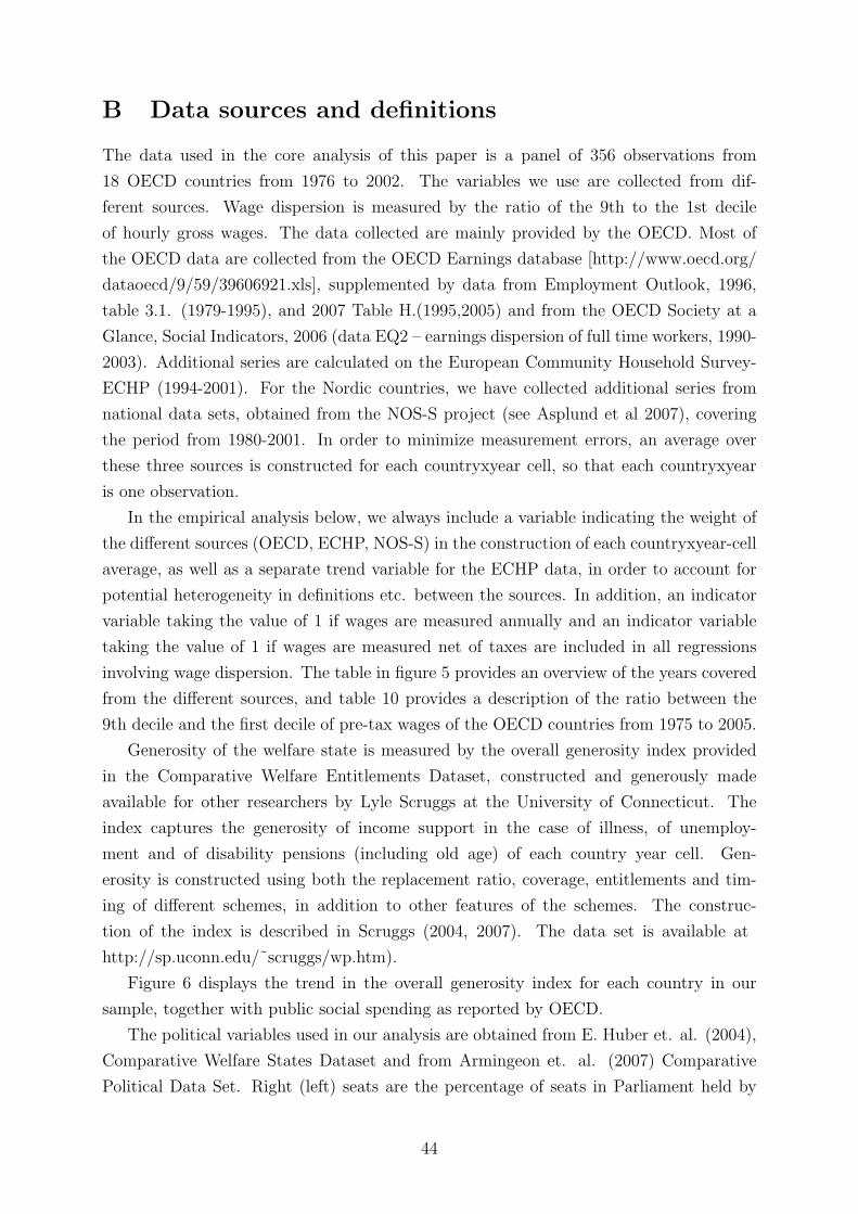
B Data sources and definitions

The data used in the core analysis of this paper is a panel of 356 observations from

18 OECD countries from 1976 to 2002. The variables we use are collected from dif-

ferent sources. Wage dispersion is measured by the ratio of the 9th to the 1st decile

of hourly gross wages. The data collected are mainly provided by the OECD. Most of

the OECD data are collected from the OECD Earnings database [http://www.oecd.org/

dataoecd/9/59/39606921.xls], supplemented by data from Employment Outlook, 1996,

table 3.1. (1979-1995), and 2007 Table H.(1995,2005) and from the OECD Society at a

Glance, Social Indicators, 2006 (data EQ2 – earnings dispersion of full time workers, 1990-

2003). Additional series are calculated on the European Community Household Survey-

ECHP (1994-2001). For the Nordic countries, we have collected additional series from

national data sets, obtained from the NOS-S project (see Asplund et al 2007), covering

the period from 1980-2001. In order to minimize measurement errors, an average over

these three sources is constructed for each countryxyear cell, so that each countryxyear

is one observation.

In the empirical analysis below, we always include a variable indicating the weight of

the different sources (OECD, ECHP, NOS-S) in the construction of each countryxyear-cell

average, as well as a separate trend variable for the ECHP data, in order to account for

potential heterogeneity in definitions etc. between the sources. In addition, an indicator

variable taking the value of 1 if wages are measured annually and an indicator variable

taking the value of 1 if wages are measured net of taxes are included in all regressions

involving wage dispersion. The table in figure 5 provides an overview of the years covered

from the different sources, and table 10 provides a description of the ratio between the

9th decile and the first decile of pre-tax wages of the OECD countries from 1975 to 2005.

Generosity of the welfare state is measured by the overall generosity index provided

in the Comparative Welfare Entitlements Dataset, constructed and generously made

available for other researchers by Lyle Scruggs at the University of Connecticut. The

index captures the generosity of income support in the case of illness, of unemploy-

ment and of disability pensions (including old age) of each country year cell. Gen-

erosity is constructed using both the replacement ratio, coverage, entitlements and tim-

ing of different schemes, in addition to other features of the schemes. The construc-

tion of the index is described in Scruggs (2004, 2007). The data set is available at

http://sp.uconn.edu/˜scruggs/wp.htm).

Figure 6 displays the trend in the overall generosity index for each country in our

sample, together with public social spending as reported by OECD.

The political variables used in our analysis are obtained from E. Huber et. al. (2004),

Comparative Welfare States Dataset and from Armingeon et. al. (2007) Comparative

Political Data Set. Right (left) seats are the percentage of seats in Parliament held by

44

Table 10: Wage Inequality. D9/D1 Ratio, 1975-2005.

Country Dataset 1975-1979 1980-1984 1985-1989 1990-1994 1995-1999 2000-2004 2005 Australia* OECD 2.64 2.88 2.83 2.83 2.94 3.08 3.12 Austria* OECD 3.45 3.51 3.56 3.23 3.26 ECHP 2.41 2.14 Belgium* OECD 2.41 2.28 1.96 1.97 ECHP 2.06 2.04 Canada* OECD 4.02 4.45 4.21 3.56 3.65 3.74 Chzechia OECD 2.40 2.74 2.84 2.99 3.10 Denmark* OECD 2.17 2.18 2.16 2.47 2.58 2.64 NOS-S 1.98 2.03 2.05 2.09 2.13 ECHP 1.87 1.86 Finland* OECD 2.65 2.49 2.50 2.39 2.36 2.43 2.42 NOS-S 2.74 2.71 2.54 2.66 ECHP 2.20 2.18 France* OECD 3.35 3.18 3.19 3.21 3.07 2.98 2.91 ECHP 2.88 2.87 Germany* OECD 2.88 2.86 2.78 2.93 3.07 3.26 ECHP 2.88 Greece OECD 1.80 ECHP 2.70 2.75 Hungary OECD 2.84 3.70 4.13 4.37 4.46 Iceland NOS-S 2.97 3.19 3.29 Ireland* OECD 4.06 3.97 3.59 3.57 ECHP 2.99 2.68 Italy* OECD 2.94 2.55 2.28 2.35 2.40 ECHP 2.05 2.02 Japan* OECD 3.00 3.08 3.15 3.07 2.99 2.96 3.12 Korea OECD 4.59 4.25 3.75 3.77 4.04 4.48 Netherlands* OECD 2.57 2.47 2.55 2.60 2.83 2.91 2.91 ECHP 2.16 2.23 New Zealand* OECD 2.17 2.16 2.29 2.57 2.72 2.79 Norway* OECD 2.06 2.16 1.98 1.94 2.06 2.21 NOS-S 2.11 2.10 2.06 2.01 2.03 Poland OECD 2.59 2.65 3.03 3.49 4.05 4.31 Portugal OECD 3.56 3.85 3.07 ECHP 3.09 2.98 Spain OECD 4.22 3.53 3.53 ECHP 3.13 3.02 Sweden* OECD 2.13 2.01 2.09 2.11 2.23 2.31 2.33 NOS-S 1.81 1.74 1.82 1.94 Switzerland* OECD 2.71 2.56 3.01 2.61 United Kingdom* OECD 2.94 3.09 3.30 3.39 3.46 3.52 3.62 United States* OECD 3.75 3.91 4.23 4.40 4.57 4.66 4.86 OECD average OECD 2.89 2.92 2.93 3.02 3.06 3.11 3.30

Note: Five years averages of available data. Each cell does not necessarily represent data from each ofthe five years of the interval. (*) indicates that a country is one of the 18 countries included in the mainanalysis in this paper (due to availability of the welfare generosity score). OECD average is an averageof the figures obtained from OECD sources.

45

Figure 5: Wage Data Sources

OECD Earnings Database 08(*)

Employment Outlook 96

Socity at a Glance 06 ECHP NOS-S

Australia 76-95, 97-03 Austria 80,87-94 95-01

Belgium 85-93 99-03 95-01 Canada 81,86,88,90-94, 97-03

Denmark 80-90, 96-03 95-01 80-01 Finland 80,83,86-03 77 96-01 83,87,89,91,93,95,97-03

France 76-98, 00-03 95-01 Germany 84-03 95,96

Ireland 94, 97, 00, 03   95-01 Italy 86-96 79-84 95-01

Japan 75-03 Netherlands 77-03 95-01

New Zealand 82,84,86,88,90,92,94-03 Norway 97-03 80,83,87,91 80,83,87,91,95,97,00,03

Portugal 85,89,91-93 01-03 95-01 Spain 95,02 95-01

Sweden 75,78,80-03 86-02 Switzerland 96,98,00,02 91-03 United Kingdom 76-03

United States 76-03 * OECD Earnings Database figures have been supplemented with data from Employment Outlook 2007 for 1995 when missing. NOS-S are figures reported by Asplund et al (2008).

right (left) parties taken from Huber et al 1976-2000 and supplemented by data from

Armingeon et al for 2001-2003. Right (left) government is the five year average of an

(present and lagged) indicator variable taking the value of one if the right (left) parties

has a majority in government (g.t. 50 percent), constructed from the variable govright

(left) of Armingeon et al (2007) (defined as right (left)-wing parties in percentage of

total cabinet posts, weighted by days). Population, the employment rate of the 16-64

population as well as the share of elderly in the population are taken from Armingeon et

al (2007).

Bargaining indicators: Union density and bargaining coordination from 1976-2000 are

obtained from: Golden, Miriam; Peter Lange; and Michael Wallerstein. 2006. ”Union

Centralization among Advanced Industrial Societies: An Empirical Study.” Dataset from

http://www.shelley.polisci.ucla.edu/, version dated June 16, 2006, now available at

http://dvn.iq.harvard.edu/dvn/dv/golden/faces/study/StudyPage.jsp?studyId=636&tab=files.

Union density is defined as net density (see Ebbinghaus and Visser, 2000); 2001 and 2002 values

are set at 2000 level. Figures for Ireland, New Zealand, and Portugal from OECD Employment

Outlook 2004 table 3.3 (linearized decennial values) Coordination in bargaining is defined as the

ten year average of (present and lagged) bargaining level 2 from Golden et al (2006). Bargaining

level 2 is the level at which wages are determined, coded as follows:

1 = plant-level wage-setting

2 = industry-level wage-setting without sanctions

3 = industry-level wage-setting with sanctions

46

Figure 6: Trends in Welfare Generosity.

1020

3040

5010

2030

4050

1020

3040

5010

2030

4050

1980 1990 2000 2010 1980 1990 2000 2010 1980 1990 2000 2010 1980 1990 2000 2010 1980 1990 2000 2010

Australia Austria Belgium Canada Denmark

Finland France Germany Ireland Italy

Japan Netherland New Zealand Norway Portugal

Spain Sweden Switzerland United Kingdom United States

Overall Generostiy Index Publ. Soc. Spending (OECD)

year

Graphs by country

Note: Source; Overall Generosity Index: The Comparative Welfare Entitlements Dataset by Lyle Scruggs,University of Connecticut. Public Social Spending: OECD Social Expenditure Database.

4 = central wage-setting without sanctions

5 = central wage-setting with sanctions

2001-2002 values of bargaining level 2 are set at 2000 values. Figures for Ireland, New

Zealand and Portugal from OECD Employment Outlook 2007 table 3.5 Centralisation index.

Openness is defined as 100x(export+import)/2gdp (openk/2) from Penn World Tables, ver-

sion 6.2 (see Alan Heston, Robert Summers and Bettina Aten, 2006). gdp per capita (USD,

PPP-adjusted) is taken from OECD Factbook 2006: Economic, Environmental and Social Statis-

tics. The percent of population with tertiary education from 1990-2003 is taken from OECD

Education at a Glance, various years (linearised when missing). From 1976-1989 data is imputed

using linearised values of five years figures reported in Delafuente and Domenech (2002).

The following country classification, which is based on Esbing-Andersen’s (1990) decommod-

ification index with some modifications (see eg. Scruggs, 2007), is used illustratively throughout:

Liberal countries: Australia, Canada, Ireland, New Zealand, United Kingdom, United States.

Conservative countries: Finland, France, Germany, Italy, Japan, Portugal, Spain, Switzer-

land.

Social Democratic countries: Austria, Belgium, Denmark, Netherlands, Norway, Sweden.

Sources for the US-analysis 1945-2001: Social Transfers 1945-1959, Historical Statistics of

the United States, Millennial edition (includes Social insurance, public aid, health and medial

programs, veterans programs, housing and other social welfare programs, tables Bf189-195/gdp

table Ca1); 1960-2001 from the OECD Lindert-Allard Data Set (2009). d9d1 from Goldin

and Katz (2007) Figure 5: 1945-1960 Census data (interpolation for 45-48 (from 1939), 50-

47

58, and 60-62. CPS-March data from 1963. Unemployment : 1940 Historical Statistics of the

United States, Millennial edition, BA352. 1941 Interpolation. 1942-1969 Bureau of Labor

Statistics, Annual household data, employment data statistics. 1970 - 2001 Source: OECD

(2007), OECD Main Economic Indicators, April, Paris. Table A. Share of Population 65 +

: Historical Statistics of the United States, Millennial edition, Table Aa139. Right Govern-

ment : 5 year average of an (present and lagged) indicator variable for a Republican Presi-

dent. Source: Armingeon et al (2007). Union density : 1940-1950 from Historical Statistics

of the US Millenial ed. Series Ba4791. College attainment : 4 years or more of college: US

Census http://www.census.gov/population/ www/socdemo/educ-attn.html, Linear interpola-

tion 41-49, 51-59, 61, 63, 65, 94. Real Federal Minimum Wage: 1940-59 USGovinfo, cpi adj.

http://usgovinfo.about.com/ library/blminwage.htm. 1960-2001 OECD Stat.: Real hourly min-

imum wage.

B.1 Negative Correlation between Inequality and Generosity

Figure 1 in the introduction shows that countries with high wage inequality tend to have lower

welfare generosity scores. Here we check the robustness of this negative association, first by using

various measures of both inequality and generosity and secondly by calculating the correlation

between the residuals of the two variables in a simple regression framework.

In figures 7 and 8 we ensure ourselves that the negative association is not simply due to

the particular measures we have chosen to represent inequality and generosity. In figure 7 we

measure the overall generosity index on the y-axis of each figure, while we vary the inequality

measure on the x-axis.

The first panel shows the log of the d9 d1 ratio. The next panel displays d9d1 directly. The

next two panels show more detailed measures of wage dispersion, utilizing different dimensions of

the data calculated from quantile regressions. These observations constitute a panel of estimates

from separate micro data sets for each country-year of 11 European countries (see note to the

figure for details). The first; within group wage inequality, shows the interquartile range between

d9 and d1 of conditional wages for men with tertiary education, within the same age group

working in private manufacturing (see note to the figure for details). The second shows between

group wage inequality; measured as the wage premium associated with tertiary education in

median Mincer regressions.

The last two panels show measures of household income rather than individual wages. The

first shows the gini coefficient of gross household income from Deininger and Squire (1996) while

the last panel shows d9d1 ratio of disposable household income calculated from the Luxembourg

Income Study.

Figure 8 plots our preferred measure of wage inequality against different measures of welfare

generosity and public welfare spending. Again we find a consistent negative pattern between

welfare generosity and wage dispersion. Simple regression analyses (not shown), including year

dummies, confirm that the downward slope displayed in all panels of figures 3 and 4 display

statistically significant downward patterns.

Countries with high wage inequality tend to have lower welfare generosity scores as the figures

48

Figure 7: Measures of Inequality.

1020

3040

50O

vera

ll G

ener

osity

Inde

x

.6 .8 1 1.2 1.4 1.6ln(d9/d1)

1020

3040

50O

vera

ll G

ener

osity

Inde

x

2 3 4 5Wage Dispersion (d9/d1)

1020

3040

50O

vera

ll G

ener

osity

Inde

x

.4 .6 .8 1 1.2Within-tertiary d9d1

1020

3040

50O

vera

ll G

ener

osity

Inde

x

.2 .4 .6 .8Tertiary wage premium

1020

3040

50O

vera

ll G

ener

osity

Inde

x

20 25 30 35 40Gini Gross Household Income

1020

3040

50O

vera

ll G

ener

osity

Inde

x

2 3 4 5 6d9d1 Household Disp. Income

Source; Y-axis: Overall Generosity Index from The Comparative Welfare Entitlements Dataset by LyleScruggs, University of Connecticut. X-axis: Panels a and b use wage inequality measures from our data,mainly from OECD sources, see data section for details. Panel c and d display wage inequality measurescalculated from quantile regressions from a panel of 11 European countries (Aut, Bel, Den, Fin, Fra, Ger,Ita, Nor, Swe, UK; N=79, years 19080-2002) by the EDWIN project (see www.etla.fi/edwin). Panel cdisplays the d9-d1 interquantile range of the conditional wage distribution, calculated for individuals withcompleted tertiary education, of the same age, gender, and within private sector manufacturing. Panel ddisplays the wage premium associated with tertiary education from q5 of the same quantile regression.Panel e displays the gini coefficient of gross household income from the Deininger and Squire (1996) data.Contries included are Aus, Aut, Bel, Can, Den, Fin, Fra, Ger, Ita, Jap, NZ, Nor, Swe, UK, US; N=93, years 1976-1992. Panel f shows the d9d1 ratio of disposable household income from the LuxembourgIncome Study, countries included are Aus, Aut, Bel, Can, Den, Fin, Fra, Ger, Ire, Ita, Net, Nor, Swe,UK, US; N= 93, years 1976-1992.

49

Figure 8: Measures of Generosity.

23

45

Wag

e D

ispe

rsio

n (d

9/d1

)

2.5 3 3.5 4ln(Overall G-Index)

23

45

Wag

e D

ispe

rsio

n (d

9/d1

)

10 15 20 25 30 35Public Social Spending

23

45

Wag

e D

ispe

rsio

n (d

9/d1

)

5 10 15 20 25 30Social Transfers

23

45

Wag

e D

ispe

rsio

n (d

9/d1

)

0 5 10 15Unempl. Generosity Index

23

45

Wag

e D

ispe

rsio

n (d

9/d1

)

0 5 10 15Sickness Generosity Index

23

45

Wag

e D

ispe

rsio

n (d

9/d1

)

5 10 15 20Pension Generosity Index

Source; Y-axis: Wage Dispersion from our own data set, mainly from OECD sources, see data sectionfor details. X-axis: Panel a use our preferred measure of generosity: ln(Overall Generosity Score) fromthe Comparative Welfare Entitlements Dataset, see data section for details. Panels b, c, and d showthe underlying indexes which add up to the overall generosity score: Panel b shows the generosityof unemployment benefits, panel c the generosity of sickness benefits, and panel d the generosity ofdisability and old age pensions. The two last panels show spending data from OECD sources (OECDSocial Spending Database), panel e gives the sum of public social spending [Countries included are Aus,Aut, Bel, Can, Den, Fin, Fra, Ger, Ire, Ita, Jap, Net, NZ, Nor, Por, Spa, Swe, UK, US; N=365, years1970-2003] and panel f shows the sum of social transfers [Contries included are Aus, Aut, Bel, Can, Den,Fin, Fra, Ger, Ire, Ita, Jap, Net, NZ, Nor, Swe, UK, US; N=79, years 1980-2002].

50

Table 11: Wage Inequality and Generosity

Descriptive regressionsSUR1 SUR2 SUR3

Generosity Inequality Generosity Inequality Generosity InequalityCoef./se Coef./se Coef./se Coef./se Coef./se Coef./se

Trend –.011* .006 –.012** .009** –.033*** .005(.005) (.004) (.004) (.003) (.004) (.003)

Trend squared –.001*** .000 –.001*** .000 –.000 .000*(.000) (.000) (.000) (.000) (.000) (.000)

log Population –.135*** .114*** –.096*** .104***(.009) (.007) (.013) (.009)

log GDP per capita .400*** .186**(.080) (.057)

Openness(pct GDP) .005*** .001(.001) (.001)

Union Density .001 –.002**(.001) (.001)

Age 65+(pct pop) .051*** –.043***(.005) (.004)

Constant 3.302*** 1.067*** 4.632*** –.093 –.752 –1.221*(.020) (.016) (.088) (.073) (.805) (.576)

R sq.inquality .044 .426 .647R sq.generosity .295 .561 .726No. of cases 356 356 356Corr. residuals –.417 –.373 –.325Chi-sq Breush-Pagan 61.9 49.4 37.6

Dependent variables:ln(Wage Dispersion) and ln(Generosity Index). Inequality equations alsoinclude data source controls (see data section).

shows. In table 11 we report descriptive regressions of wage inequality and generosity, using

standard SUR-regressions on the pooled data set. Dependent variables are ln(Wage dispersion)

and ln(Overall Generosity Index). In the first model, SUR1, we confirm a statistically significant

negative correlation between the residuals of wage inequality and welfare generosity, in line with

the patterns observed in figures 1 and 2. The correlation coefficient between the de-trended

residuals is -0.42 and highly significant.

In model SUR2 we establish that the correlation is not just due to the fact that small

countries tend to have more generous welfare states and at the same time less wage inequality.

In model SUR3 we find that the richer countries have more generous welfare states and tend

to have more inequality. Furthermore we find that more open economies have more generous

welfare states, that higher union density is associated with more generous welfare states and

more compressed wage distributions, and that the proportion of the population over 65 is pos-

itively correlated with welfare generosity and negatively associated with wage inequality. The

correlation between the residuals of the two regressions remains negative and highly significant.

C Some further robustness checks

Table 12 and 13 provide the full regression results of tables 2 and 4 in the main text. The first

two models are OLS specifications, the third model is the preferred IV-specification, used in the

second stage of our 3SLS models in table 1, and the last two models provides a check of the

validity of the instruments.

Table 15 reports the results from three different experiments involving the right government

variable as instrument. The two first models weights the government variable up if there is a

close tie in the parliament, the last model uses the lead rather than the lag of the right wing

government variable. See the main text for details and interpretation.

51

Table 12: Welfare Generosity

Dependent variable: ln(Generosity Index)OLS OLS-FIX IV-1 IV-2 IV-3

Coef./se Coef./se Coef./se Coef./se Coef./seln(Wage Dispersion) –.4938*** –.3743*** –.6343*** –.7833*** –.5083*

(.0453) (.0601) (.1315) (.2005) (.2226)Trend –.0219*** –.0226*** –.0196*** –.0171*** –.0213***

(.0027) (.0027) (.0030) (.0046) (.0033)Right cabinet [0,1] –.0341* –.0382*** –.0285* –.0223 –.0366**

(.0170) (.0111) (.0121) (.0138) (.0128)log GDP per capita .4248*** .4649*** .4452*** .4120*** .4498***

(.0503) (.0386) (.0400) (.0527) (.0403)Openness (pct GDP) .0051*** –.0032** –.0037** –.0046** –.0031**

(.0005) (.0011) (.0011) (.0015) (.0012)Age 65+ (pct pop) .0167*** .0132*** .0073 .0023 .0106*

(.0033) (.0039) (.0047) (.0068) (.0053)Union Density .0003 –.0021* –.0024** –.0026** –.0015

(.0005) (.0008) (.0009) (.0010) (.0010)Empl.pct 16-64 .0015

(.0015)Tertiary (pct pop) .0008

(.0018)Bargaining Coord. –.0088

(.0142)Workers in confl.(pct) –.0009

(.0007)Constant –.9989* –1.0704*

(.5027) (.4300)F-value fixed ctry 75.8640Sargan test p-value .2413 .0965 .1988Cragg-Donald F-value 21.85 20.15 14.47Hausman test p-value .0219 .0163 .3733P-value composition .5633P-value bargaining .2509No. of cases 356 356 356 356 356

Note: The instruments for wage inequality include Bargaining coordination, Share of workersin conflict, Share with tertiary education and the Employment rate 16-64, when not included inthe equations.

Table 13: Wage Inequality

Dep.var. ln(d9/d1)OLS OLS-FIX IV 1 IV 2 IV 3

Coef./se Coef./se Coef./se Coef./se Coef./seGenerosity –.2891*** –.2697*** –.5143*** –.5207*** –.5033**

(.0417) (.0388) (.0840) (.0854) (.1823)Bargaining Coord. –.0835*** –.0369*** –.0276** –.0294** –.0272**

(.0073) (.0087) (.0094) (.0103) (.0099)Workers in confl.(pct) –.0003 .0014** .0009* .0009 .0007

(.0007) (.0004) (.0005) (.0005) (.0007)Tertiary (pct pop) .0024 –.0001 –.0009 –.0010 –.0001

(.0013) (.0014) (.0014) (.0015) (.0017)Empl.pct 16-64 –.0007 .0028*** .0032*** .0032*** .0043***

(.0009) (.0008) (.0008) (.0008) (.0009)log GDP per capita .0145 .0959*** .1414*** .1416*** .0719

(.0286) (.0227) (.0273) (.0274) (.1200)Openness (pct GDP) –.0003 –.0021* –.0043*** –.0043*** –.0047***

(.0005) (.0008) (.0011) (.0011) (.0011)Age 65+ (pct pop) –.0138*** –.0107*** –.0095** –.0090** –.0110**

(.0033) (.0031) (.0033) (.0035) (.0041)Union Density –.0023*** –.0008 –.0007 –.0006 –.0005

(.0005) (.0008) (.0009) (.0009) (.0010)Right government[0,1] –.0046

(.0104)Year dummies Y

Constant 2.3396*** 1.0933***(.2481) (.2004)

F-value ctry.fix.eff 93.70p-value year dummies .9496Sargan test p-value .6581Cragg-Donald F-value 48.11 93.43 19.98Hausman test p-value .0004 .0004 .0523No. of cases 356 356 356 356 356

Note: The instruments for generosity in models IV1-IV3 include right cabinet and trend withthe exception of the included variable in each model. All equations include data source controls(see data section for details).

52

Table 14: E-multiplier: Different specifications

3SLS FE 3SLS FE 3SLS FEG-Index ln(W-disp.) ln(G-index) W-Dispersion G-Index W-DispersionCoef./se Coef./se Coef./se Coef./se Coef./se Coef./se

ln(W-disp.) –11.932***(3.160)

Trend –.560*** –.019*** –.549***(.073) (.003) (.078)

Right cabinet [0,1] –.798*** –.026** –.793***(.238) (.008) (.236)

log GDP per cap. 11.755*** .161*** .448*** .577*** 11.829*** .558***(.972) (.022) (.039) (.063) (.985) (.070)

Openness(pct) –.101*** –.005*** –.005*** –.019*** –.116*** –.021***(.028) (.001) (.001) (.003) (.030) (.003)

Share 65+ pct .204 –.010*** .007 –.028** .215 –.034***(.115) (.003) (.005) (.009) (.119) (.009)

Union Density –.054* –.001 –.002* –.000 –.041* .000(.021) (.001) (.001) (.002) (.021) (.002)

W-Dispersion –.196*** –3.521***(.041) (1.048)

G-Index –.021*** –.073***(.003) (.010)

Barg. Coord. –.025*** –.065** –.077***(.007) (.020) (.022)

Conflict (pct) .002*** .003*** .004**(.000) (.001) (.001)

Tertiary (pct pop) –.002* –.003 –.003(.001) (.003) (.003)

Empl.pct. 16-64 .003*** .009*** .011***(.001) (.002) (.002)

ln(G-index) –1.855***(.235)

Constant –85.773*** .302 –.845 4.038*** –88.893*** .091(13.101) (.176) (.526) (.603) (13.302) (.547)

Equality multiplier 1.332 1.573 1.345E.m l.t.1:p-value .005 .003 .009No. of cases 356 356 356

Number of countries: 18. Instruments for wage inequality included in the IV specifications areBargaining coordination, Workers in conflict, Share of pop. with tertiary education and theemployment pct(16-64). Instruments for generosity included in the IV specifications are Rightcabinet and trend. See tables 2 and 4. All models include fixed country effects.

Table 15: Robustness checks - 3SLS

Right-tied Weighted Right-leadGenerosity Inequality Generosity Inequality Generosity Inequality

Coef./se Coef./se Coef./se Coef./se Coef./se Coef./seInequality –.6315*** –.4346* –.7550***

(.1247) (.1869) (.1114)Trend –.0199*** –.0219*** –.0178***

(.0029) (.0034) (.0030)Right tied –.0348***

(.0101)Right cab.[0,1] –.0342**

(.0107)Right lead .0066

(.0085)Generosity –.5234*** –.5024*** –.4359***

(.0730) (.0696) (.0853)Barg. Coordination –.0204** –.0218** –.0302***

(.0066) (.0074) (.0069)Conflict(pct) .0015*** .0008 .0015***

(.0004) (.0005) (.0003)Tertiary (pct pop) –.0020* –.0004 –.0017

(.0010) (.0012) (.0010)Empl.pct. 16-64 .0024*** .0034*** .0026***

(.0006) (.0008) (.0006)Constant –.7955 1.4359*** –1.3337* 1.3974*** –.4380 1.3534***

(.5187) (.1896) (.6175) (.1869) (.4874) (.2028)Equality multiplier 1.4936 1.2793 1.4905E.m l.t. 1:p-value .0018 .0389 .0016No. of cases 356 337 307

Number of countries: 18. Dependent variables: ln(Overall Generosity Index) and ln(Wagedispersion). Specifications as in table 7, only endogenous variables and instruments displayed.In the first model Right Government is weighted by the Tie-variable. In the second model, thefull model is weighted by the Tie-variable. In the third model, Right government is replaced byit’s 5 year lead.

53