the engineer’s guide to - univerzita...
TRANSCRIPT
The Engineer’s Guide to
By John Watkinson
HANDBOOK
SERIES


The Engineer’s Guide to Compression
John Watkinson

© Snell & Wilcox Ltd. 1996 All rights reserved
Text and diagrams from this publication may be reproduced provided acknowledgement is
given to Snell & Wilcox.
ISBN 1 900739 06 2
Snell & Wilcox Inc.
1156 Aster Ave
Suite F
Sunnyvale, CA 94086
USA
Snell & Wilcox Ltd.
Durford Mill
Petersfield
Hampshire GU13 5AZ
United Kingdom

Contents
Section 1 - Introduction to Compression
1.1 What is compression? 1
1.2 Applications 2
1.3 How does compression work? 3
1.4 Types of compression 6
1.5 Audio compression principles 6
1.6 Video compression principles 9
1.7 Dos and don’ts 14
Section 2 - Digital Audio and Video
2.1 Digital basics 15
2.2 Sampling 17
2.3 Interlace 19
2.4 Quantizing 19
2.5 Digital video 22
2.6 Digital audio 24
Section 3 - Compression tools
3.1 Digital filters 26
3.2 Pre-filtering 28
3.3 Upconversion 31
3.4 Transforms 35
3.5 The Fourier transform 35
3.6 The Discrete Cosine Transform 40
3.7 Motion estimation 42

Section 4 - Audio compression
4.1 When to compress audio 50
4.2 The basic mechanisms 50
4.3 Sub-band coding 51
4.4 Transform coding 56
4.5 Audio compression in MPEG 58
4.6 MPEG Layers 59
Section 5 - Video compression
5.1 Spatial and temporal redundancy 62
5.2 The Discrete Cosine Transform 62
5.3 Weighting 64
5.4 Variable length coding 65
5.5 Intra-coding 65
5.6 Inter-coding 66
5.7 Motion compensation 68
5.8 I pictures 71
Section 6 - MPEG
6.1 Applications of MPEG 73
6.2 Profiles and Levels 74
6.3 MPEG-1 and MPEG-2 76
6.4 Bi-directional coding 76
6.5 Data types 78
6.6 MPEG bitstream structure 78
6.7 Systems layer 80

John Watkinson
John Watkinson is an independent author, journalist and consultant in the
broadcasting industry with more than 20 years of experience in research
and development
With a BSc (Hons) in Electronic Engineering and an MSc in Sound and
Vibration, he has held teaching posts at a senior level with The Digital
Equipment Corporation, Sony Broadcasting and Ampex Ltd., before
forming his own consultancy.
Regularly delivering technical papers at conferences included AES,
SMPTE, IEE, ITS and Montreux, John Watkinson has also written
numerous publications including “The Art of Digital Video”,
“The Art of Digital Audio” and “The Digital video Tape Recorder”.
Other publications written by John Watkinson in the Snell and Wilcox
Handbook series include: “The Engineer’s Guide to Standards
Conversion”, “The Engineer’s Guide to Decoding and Encoding”,
“The Engineer’s Guide to Motion Compensation” and
“Your Essential Guide to Digital”.

Section 1 - Introduction to CompressionIn this section we discuss the fundamental characteristics of compression
and see what we can and cannot expect without going into details which
come later.
1.1 What is compression?
Normally all audio and video program material is limited in its quality by
the capacity of the channel it has to pass through. In the case of analog
signals, the bandwidth and the signal to noise ratio limit the channel. In the
case of digital signals the limitation is the sampling rate and the sample
wordlength, which when multiplied together give the bit rate.
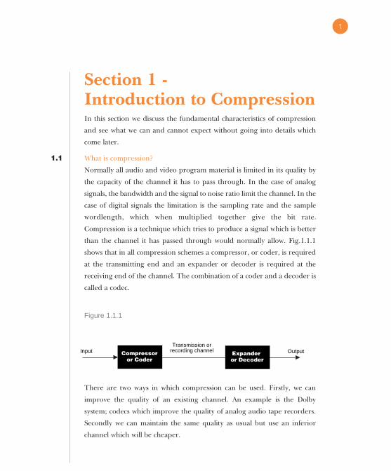
Compression is a technique which tries to produce a signal which is better
than the channel it has passed through would normally allow. Fig.1.1.1
shows that in all compression schemes a compressor, or coder, is required
at the transmitting end and an expander or decoder is required at the
receiving end of the channel. The combination of a coder and a decoder is
called a codec.
Figure 1.1.1
There are two ways in which compression can be used. Firstly, we can
improve the quality of an existing channel. An example is the Dolby
system; codecs which improve the quality of analog audio tape recorders.
Secondly we can maintain the same quality as usual but use an inferior
channel which will be cheaper.
Expander or Decoder
Input OutputCompressoror Coder
Transmission orrecording channel
1

Bear in mind that the word compression has a double meaning. In audio,
compression can also mean the deliberate reduction of the dynamic range
of a signal, often for radio broadcast purposes. Such compression is single
ended; there is no intention of a subsequent decoding stage and
consequently the results are audible.
We are not concerned here with analog compression schemes or single
ended compressors. We will be dealing with digital codecs which accept
and output digital audio and video signals at the source bit rate and pass
them through a channel having a lower bit rate. The ratio between the
source and channel bit rates is called the compression factor.
1.2 Applications
For a given quality, compression lowers the bit rate, hence the alternative
term of bit-rate reduction (BRR). In broadcasting, the reduced bit rate
requires less bandwidth or less transmitter power or both, giving an
economy. With increasing pressure on the radio spectrum from other
mobile applications such as telephones developments such as DAB (digital
audio broadcasting) and DVB (digital video broadcasting) will not be viable
without compression. In cable communications, the reduced bit rate lowers
the cost.
In recording, the use of compression reduces the amount of storage medium
required in direct proportion to the compression factor. For archiving, this
reduces the cost of the library. For ENG (electronic news gathering)
compression reduces the size and weight of the recorder. In disk based
editors and servers for video on demand (VOD) the current high cost of disk
storage is offset by compression. In some tape storage formats, advantage is
taken of the reduced data rate to relax some of the mechanical tolerances.
Using wider tracks and longer wavelengths means that the recorder can
function in adverse environments or with reduced maintenance.
2
1.3 How does compression work?
In all conventional digital audio and video systems the sampling rate, the
wordlength and the bit rate are all fixed. Whilst this bit rate puts an upper
limit on the information rate, most real program material does not reach
that limit. As Shannon said, any signal which is predictable contains no
information. Take the case of a sinewave: one cycle looks the same as the
next and so a sinewave contains no information. This is consistent with the
fact that it has no bandwidth. In video, the presence of recognisable objects
in the picture results in sets of pixels with similar values. These have spatial
frequencies far below the maximum the system can handle. In the case of
a test card, every frame is the same and again there is no information flow
once the first frame has been sent.
The goal of a compressor is to identify and send on the useful part of the
input signal which is known as the entropy. The remaining part of the
input signal is called the redundancy. It is redundant because it can be
predicted from what the decoder has already been sent.
Some caution is required when using compression because redundancy
can be useful to reconstruct parts of the signal which are lost due to
transmission errors. Clearly if redundancy has been removed in a
compressor the resulting signal will be less resistant to errors. unless a
suitable protection scheme is applied.
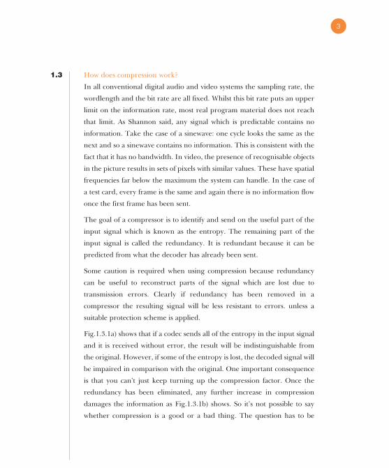
Fig.1.3.1a) shows that if a codec sends all of the entropy in the input signal
and it is received without error, the result will be indistinguishable from
the original. However, if some of the entropy is lost, the decoded signal will
be impaired in comparison with the original. One important consequence
is that you can’t just keep turning up the compression factor. Once the
redundancy has been eliminated, any further increase in compression
damages the information as Fig.1.3.1b) shows. So it’s not possible to say
whether compression is a good or a bad thing. The question has to be
3

qualified: how much compression on what kind of material and for what
audience?
Figure 1.3.1
As the entropy is a function of the input signal, the bit rate out of an ideal
compressor will vary. It is not always possible or convenient to have a
variable bit rate channel, so many compressors have a buffer memory at
each end of a fixed bit rate channel. This averages out the data flow, but
causes more delay. For applications such as video-conferencing the delay is
unacceptable and so fixed bit rate compression is used to aviod the need
for a buffer.
So far we have only considered an ideal compressor which can perfectly
sort the entropy from the redundancy. Unfortunately such a compressor
would have infinite complexity and have an infinite processing delay. In
practice we have to use real, affordable compressors which must fail to be
WordlengthEntropy
Redundancy
Sampling rate
a) Perfectcompressor
b) Excesscompression
c) Practicalcompressor
Not all entropysent - quality loss
All entropy sent- no quality loss
4

ideal by some margin. As a result the compression factors we can use have
to be reduced because if the compressor can’t decide whether a signal is
entropy or not it has to be sent just in case. As Fig.1.3.1c) shows, the
entropy is surrounded by a “grey area” which may or may not be entropy.
The simpler and cheaper the compressor, and the shorter its encoding
delay, the larger this grey area becomes. However, the decoder must be
able to handle all of these cases equally well. Consequently compression
schemes are designed so that all of the decisions are taken at the coder. The
decoder then makes the best of whatever it receives. Thus the actual bit
rate sent is determined at the coder and the decoder needs no adjustment.
Clearly, then, there is no such thing as the perfect compressor. For the
ultimate in low bit rates, a complex and therefore expensive compressor is
needed. When using a higher bit rate a simpler compressor would do. Thus
a range of compressors is required in real life. Consequently MPEG is not a
standard for a compressor, nor is it a standard for a range of compressors.
MPEG is a set of standards describing a range of bitstreams which
compliant decoders must be able to handle. MPEG does not specify how
these bitstreams are to be created. There are a number of advantages to
this approach. A wide variety of compressors, some using proprietary
techniques, can produce bitstreams compatible with any compliant
decoder. There can be a range of compressors at different points on the
price/performance scale. There can be competition between vendors.
Research may reveal better ways of encoding the bit stream, producing
improved quality without making the decoders obsolete.
When testing an MPEG codec, it must be tested in two ways. Firstly it must
be compliant. This is a yes/no test. Secondly the picture and/or sound
quality must be assessed. This is much more difficult task because it is
subjective.
5

1.4 Types of compression
Compression techniques exist which treat the input as an arbitrary data
stream and compress by identifying frequent bit patterns. These codecs can
be bit accurate; in other words the decoded data are bit-for-bit identical
with the original. Such coders, called lossless coders, are essential for
compressing computer data and are used in so called ‘stacker’ programs
which increase the capacity of disk drives. However, stackers can only
achieve a limited compression factor and are not appropriate for audio and
video where bit accuracy is not essential.
In audio and video, the human viewer or listener will be unable to detect
certain small discrepancies in the signal due to the codec. However, the
admission of these small discrepancies allows a great increase in the
compression factor which can be achieved. Such codecs can be called near-
lossless. Although they are not bit accurate, they are sufficiently accurate
that humans would not know the difference. The trick is to create coding
errors which are of a type which we perceive least. Consequently the coder
must understand the human sensory system so that it knows what it can
get away with. Such a technique is called perceptual coding. The higher
the compression factor the more accurately the coder needs to mimic
human perception.
1.5 Audio compression principles
Audio compression relies on an understanding of the hearing mechanism
and so is a form of perceptual coding. The ear is only able to extract a
certain proportion of the information in a given sound. This could be
called the perceptual entropy, and all additional sound is redundant. The
basilar membrane in the ear behaves as a kind of spectrum analyser; the
part of the basilar membrane which resonates as a result of an applied
sound is a function of frequency. The high frequencies are detected at the
end of the membrane nearest to the eardrum and the low frequencies are
detected at the opposite end. The ear analyses with frequency bands,
6

known as critical bands, about 100 Hz wide below 500 Hz and from one-
sixth to one-third of an octave wide, proportional to frequency, above this.
The ear fails to register energy in some bands when there is more energy
in a nearby band. The vibration of the membrane in sympathy with a single
frequency cannot be localised to an infinitely small area, and nearby areas
are forced to vibrate at the same frequency with an amplitude that
decreases with distance. Other frequencies are excluded unless the
amplitude is high enough to dominate the local vibration of the
membrane. Thus the membrane has an effective Q factor which is
responsible for the phenomenon of auditory masking, in other words the
decreased audibility of one sound in the presence of another. The
threshold of hearing is raised in the vicinity of the input frequency. As
shown in Fig.1.5.1, above the masking frequency, masking is more
pronounced, and its extent increases with acoustic level. Below the
masking frequency, the extent of masking drops sharply.
Figure 1.5.1
Threshold of hearing
Masking tone
Skirts of thresholddue to masking
Level
Level
Frequency
Frequency
7

Because of the resonant nature of the membrane, it cannot start or stop
vibrating rapidly; masking can take place even when the masking tone
begins after and ceases before the masked sound. This is referred to as
forward and backward masking.
Audio compressors work by raising the noise floor at frequencies where the
noise will be masked. A detailed model of the masking properties of the ear
is essential to their design. The greater the compression factor required,
the more precise the model must be. If the masking model is inaccurate, or
not properly implemented, equipment may produce audible artifacts.
There are many different techniques used in audio compression and these
will often be combined in a particular system.
Predictive coding uses circuitry which uses a knowledge of previous
samples to predict the value of the next. It is then only necessary to send
the difference between the prediction and the actual value. The receiver
contains an identical predictor to which the transmitted difference is added
to give the original value. Predictive coders have the advantage that they
work on the signal waveform in the time domain and need a relatively
short signal history to operate. They cause a relatively short delay in the
coding and decoding stages.
Sub-band coding splits the audio spectrum up into many different
frequency bands to exploit the fact that most bands will contain lower level
signals than the loudest one.
In spectral coding, a transform of the waveform is computed periodically.
Since the transform of an audio signal changes slowly, it need be sent much
less often than audio samples. The receiver performs an inverse transform.
Most practical audio coders use some combination of sub-band or spectral
coding. Re-quantizing of sub-band samples or transform coefficients causes
increased noise which the coder places at frequencies where it will be
masked. Section 4 will treat these ideas in more detail.
8

If an excessive compression factor is used, the coding noise will exceed the
masking threshold and become audible. If a higher bit rate is impossible,
better results will be obtained by restricting the audio bandwidth prior to
the encoder using a pre-filter. Reducing the bandwidth with a given bit
rate allows a better signal to noise ratio in the remaining frequency range.
Many commercially available audio coders incorporate such a pre-filter.
1.6 Video compression principles
Video compression relies on two basic assumptions. The first is that human
sensitivity to noise in the picture is highly dependent on the frequency of
the noise. The second is that even in moving pictures there is a great deal
of commonality between one picture and the next. Data can be conserved
by raising the noise level where it cannot be detected and by sending only
the difference between one picture and the next.
Fig.1.6.1 shows that in a picture, large objects result in low spatial
frequencies (few cycles per unit distance) whereas small objects result in
high spatial frequencies (many cycles per unit distance). Fig.1.6.2 shows
that human vision detects noise at low spatial frequencies much more
readily than at high frequencies. The phenomenon of large-area flicker is
an example of this.
Figure 1.6.1
High frequencyLow frequency
LargeObject
SmallObject
9

Figure 1.6.2
Compression works by shortening or truncating the wordlength of data
words. This reduces their resolution, raising noise. If this noise is to be
produced in a way which minimises its visibility, the truncation must vary
with spatial frequency. Practical video compressors must perform a spatial
frequency analysis on the input, and then truncate each frequency
individually in a weighted manner. Such a spatial frequency analysis also
reveals that in many areas of the picture, only a few frequencies dominate
and the remainder are largely absent. Clearly where a frequency is absent
no data need be transmitted at all. Fig.1.6.3 shows a simple compressor
working on this principle. The decoder is simply a reversal of the
frequency analysis, performing a synthesis or inverse transform process.
Section 3 explains how frequency analysis works.
Figure 1.6.3
Transform
Video out
Video inWeighting
Truncatecoefficients & discard
zeros
Inverse Weight
InverseTransform
Coefficients
Visibilityof noise
Spatial frequency
10
The simple concept of Fig.1.6.3 treats each picture individually and is
known as intra-coding. Compression schemes designed for still images,
such as JPEG (Joint Photographic Experts Group) have to work in this way.
For moving pictures, exploiting redundancy between pictures, known as
inter-coding, gives a higher compression factor.
Fig.1.6.4 shows a simple inter-coder. Starting with an intra-coded picture,
the subsequent pictures are described only by the way in which they differ
from the one before. The decoder adds the differences to the previous
picture to produce the new one. The difference picture is produced by
subtracting every pixel in one picture from the same pixel in the next
picture. This difference picture is an image in its own right and can be
compressed with an intra-coding process of the kind shown in Fig.1.6.3.
11
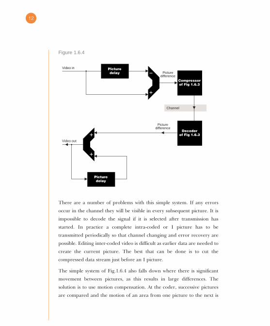
Figure 1.6.4
There are a number of problems with this simple system. If any errors
occur in the channel they will be visible in every subsequent picture. It is
impossible to decode the signal if it is selected after transmission has
started. In practice a complete intra-coded or I picture has to be
transmitted periodically so that channel changing and error recovery are
possible. Editing inter-coded video is difficult as earlier data are needed to
create the current picture. The best that can be done is to cut the
compressed data stream just before an I picture.
The simple system of Fig.1.6.4 also falls down where there is significant
movement between pictures, as this results in large differences. The
solution is to use motion compensation. At the coder, successive pictures
are compared and the motion of an area from one picture to the next is
Picturedelay
Compressorof Fig 1.6.3
Decoderof Fig 1.6.3
Picturedelay
Video out
Picturedifference
Channel
Picturedifference
Video in
12

measured to produce motion vectors. Fig.1.6.5 shows that the coder
attempts to model the object in its new position by shifting pixels from the
previous picture using the motion vectors. Any discrepancies in the process
are eliminated by comparing the modelled picture with the actual picture.
Figure 1.6.5
The coder sends the motion vectors and the discrepancies. The decoder
shifts the previous picture by the vectors and adds the discrepancies to
produce the next picture. Motion compensated coding allows a higher
compression factor and this outweighs the extra complexity in the coder
and the decoder. More will be said on the topic in section 5.
PicturedelayVideo in
Motionmeasure
Pictureshifter
Compressorof Fig 1.6.3
Decoderof Fig 1.6.3
Picture shifter
Picturedelay
Shifted previouspicture
Video out
Currentpicture
Previouspicture Shifted
previouspicture (P picture)
Picturedifference
Vectors
Channel
Previousoutput picture
Picturedifference
Vectors
13
1.7 Dos and don’ts
You don’t have to understand the complexities of compression if you stick
to the following rules:-
1. If compression is not necessary don’t use it.
2. If compression has to be used, keep the compression factor as mild as
possible; i.e. use the highest practical bit rate.
3. Don’t cascade compression systems. This causes loss of quality and the
lower the bit rates, the worse this gets. Quality loss increases if any post
production steps are performed between codecs.
4. Compression systems cause delay and make editing more difficult.
5. Compression systems work best with clean source material. Noisy
signals, tape hiss, film grain and weave or poorly decoded composite
video give poor results.
6. Compressed data are generally more prone to transmission errors
than non-compressed data.
7. Only use low bit rate coders for the final delivery of post produced
signals to the end user. If a very low bit rate is required, reduce the
bandwidth of the input signal in a pre-filter.
8. Compression quality can only be assessed subjectively.
9. Don’t believe statements comparing video codec performance to “VHS
quality” or similar. Compression artifacts are quite different to the
artifacts of consumer VCRs.
10. Quality varies wildly with source material. Beware of “convincing”
demonstrations which may use selected material to achieve low bit
rates. Use your own test material, selected for a balance of difficulty.
14
Section 2 - Digital Audio and VideoIn this section we review the formats of digital audio and video signals
which will form the input to compressors.
2.1 Digital basics
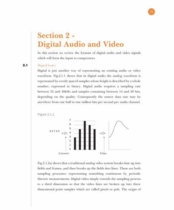
Digital is just another way of representing an existing audio or video
waveform. Fig.2.1.1 shows that in digital audio the analog waveform is
represented by evenly spaced samples whose height is described by a whole
number, expressed in binary. Digital audio requires a sampling rate
between 32 and 48kHz and samples containing between 14 and 20 bits,
depending on the quality. Consequently the source data rate may be
anywhere from one half to one million bits per second per audio channel.
Figure 2.1.1
Fig.2.1.2a) shows that a traditional analog video system breaks time up into
fields and frames, and then breaks up the fields into lines. These are both
sampling processes: representing something continuous by periodic
discrete measurements. Digital video simply extends the sampling process
to a third dimension so that the video lines are broken up into three
dimensional point samples which are called pixels or pels. The origin of
3 5 7 6 5
Convert Fi l ter
0
1
2
3
4
5
6
7
15

these terms becomes obvious when you try to say “picture cells” in a hurry.
Fig.2.1.2b) shows a television frame broken up into pixels. A typical 625/50
frame contains over a third of a million pixels. In computer graphics the
pixel spacing is often the same horizontally as it is vertically, giving the so
called “square pixel”. In broadcast video systems pixels are not quite
square for reasons which will become clearer later in this section.
Once the frame is divided into pixels, the variable value of each pixel is
then converted to a number. Fig.2.1.2c) shows one line of analog video
being converted to digital. This is the equivalent of drawing it on squared
paper. The horizontal axis represents the number of the pixel across the
screen which is simply an incremental count. The vertical axis represents
the voltage of the video waveform by specifying the number of the square
it occupies in any one pixel. The shape of the waveform can be sent
elsewhere by describing which squares the waveform went through. As a
result the video waveform is represented by a stream of whole numbers, or
to put it another way, a data stream.
16

Figure 2.1.2
In the case of component analog video there will be three simultaneous
waveforms per channel. Three converters are required to produce three
data streams in order to represent GBR or colour difference components.
Composite video can be thought of as an analog compression technique as
it allows colour in the same bandwidth as monochrome. Whilst digital
compression schemes do exist for composite video, these effectively put two
compressors in series which is not a good idea. Consequently the
compression factor has to be limited in composite systems. MPEG is
designed only for component signals and is effectively a modern
replacement for composite video which will not be considered further
here.
2.2 Sampling
Sampling theory requires a sampling rate of at least twice the bandwidth of
the signal to be sampled. In the case of a broadband signal, i.e. one in which
there are a large number of octaves, the sampling rate must be at least twice
c)
1 Frame
1stField
a)
2ndField
Line b)
17

the highest frequency in the input. Fig.2.2.1a) shows what happens when
sampling is performed correctly. The original waveform is preserved in the
envelope of the samples and can be restored by low-pass filtering.
Figure 2.2.1a
Fig.2.2.1b) shows what happens in the case of a signal whose frequency
more than half the sampling rate in use. The envelope of the samples now
carries a waveform which is not the original. Whether this matters or not
depends upon whether we consider a broadband or a narrow band signal.
Figure 2.2.1b
In the case of a broadband signal, Fig.2.2.1b) shows aliasing; the result of
incorrect sampling. Everyone has seen stagecoach wheels stopping and
going backwards in cowboy movies. It’s an example of aliasing. The
frequency of wheel spokes passing the camera is too high for the frame rate
in use. It is essential to prevent aliasing in analog to digital converters
wherever possible and this is done by including a filter, called an anti-
aliasing filter, prior to the sampling stage.
In the case of a narrow-band signal, Fig.2.2.1b) shows a heterodyning
process which down converts the narrow frequency band to a baseband
which can be faithfully described with a low sampling rate. Re-conversion
18

to analog requires an up-conversion process which uses a band-pass filter
rather than a low-pass filter. This technique is used extensively in audio
compression where the input signal can be split into a number of sub-
bands without increasing the overall sampling rate.
2.3 Interlace
Interlace is a system in which the lines of each frame are divided into odd
and even sets known as fields. Sending two fields instead of one frame
doubles the apparent refresh rate of the picture without doubling the
bandwidth required. Interlace can be considered a form of analog
compression. Interlace twitter and poor dynamic resolution are
compression artifacts. Ideally, digital compression should be performed on
non-interlaced source material as this will give better results for the same
bit rate. Using interlaced input places two compressors in series. However,
the dominance of interlace in existing television systems means that in
practice digital compressors have to accept interlaced source material.
Interlace causes difficulty in motion compensated compression, as motion
measurement is complicated by the fact that successive fields do not
describe the same points on the picture. Producing a picture difference
from one field to another is also complicated by interlace. In compression
terminology, the difficulty caused by whether to use the term “field” or
“frame” is neatly avoided by using the term “picture”.
2.4 Quantizing
In addition to the sampling process the converter needs a quantizer to
convert the analog sample to a binary number. Fig.2.4.1 shows that a
quantizer breaks the voltage range or gamut of the analog signal into a
number of equal-sized intervals, each represented by a different number.
The quantizer outputs the number of the interval the analog voltage falls
in. The position of the analog voltage within the interval is lost, and so an
error called a quantizing error can occur. As this cannot be larger than a
19

quantizing interval the size of the error can be minimised by using
enough intervals.
Figure 2.4.1
In an eight-bit video converter there are 256 quantizing intervals because
this is the number of different codes available from an eight bit number.
This allows an unweighted SNR of about 50dB. In a ten-bit converter there
are 1024 codes available and the SNR is about 12dB better. Equipment
varies in the wordlength it can handle. Older equipment and recording
formats such as D-1 only allow eight-bit working. More recent equipment
uses ten-bit samples.
Fig.2.4.2 shows how component digital fits into eight- and ten-bit
quantizing. Note two things: analog syncs can go off the bottom of the scale
because only the active line is used, and the colour difference signals are
offset upwards so positive and negative values can be handled by the binary
number range.
Q
Q
Q
Q
n+3
n+2voltageaxis n+1
n
20
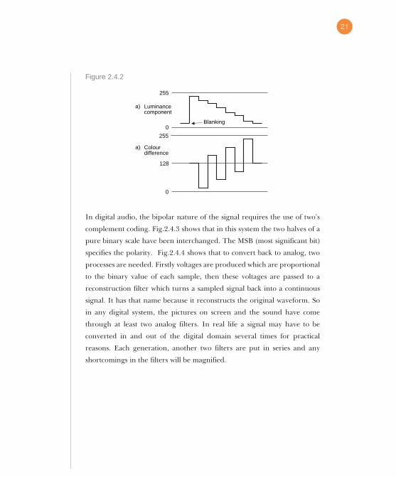
Figure 2.4.2
In digital audio, the bipolar nature of the signal requires the use of two’s
complement coding. Fig.2.4.3 shows that in this system the two halves of a
pure binary scale have been interchanged. The MSB (most significant bit)
specifies the polarity. Fig.2.4.4 shows that to convert back to analog, two
processes are needed. Firstly voltages are produced which are proportional
to the binary value of each sample, then these voltages are passed to a
reconstruction filter which turns a sampled signal back into a continuous
signal. It has that name because it reconstructs the original waveform. So
in any digital system, the pictures on screen and the sound have come
through at least two analog filters. In real life a signal may have to be
converted in and out of the digital domain several times for practical
reasons. Each generation, another two filters are put in series and any
shortcomings in the filters will be magnified.
Blanking
255
0
Luminancecomponent
a)
255
128
0
Colour difference
a)
21

Figure 2.4.3
Figure 2.4.4
2.5 Digital video
Component signals use a common sampling rate which allows 525/60 and
625/50 video to be sampled at a rate locked to horizontal sync. The figure
most often used for luminance is 13.5MHz. Fig.2.5.1 shows how the
European standard TV line fits into 13.5MHz sampling. Note that only the
active line is transmitted or recorded in component digital systems. The
digital active line has 720 pixels and is slightly longer than the analog active
line so the sloping analog blanking is always included.
Pulsed analoguesignal
Producevoltage
proportional to number
Low-passfilter
Numbers in Analogue out
1111
Blanked
Negative peak
Positive peak
111011011100101110101001100001110110010101000011001000010000
0111011001010100001100100001000011111110110111001011101010011000
22

Figure 2.5.1
In component systems, the colour difference signals have less bandwidth.
In analog components (from Betacam for example), the colour difference
signals have one half the luminance bandwidth and so we can sample them
with one half the sample rate, i.e. 6.75MHz. One quarter the luminance
sampling rate is also used, and this frequency, 3.375MHz is the lowest
practicable video sampling rate, which the standard calls 1.
So it figures that 6.75MHz is 2 and 13.5MHz is 4. Most component
production equipment uses 4:2:2 sampling. D-1, D-5 and Digital Betacam
record it, and the serial digital interface (SDI) can handle it. Fig.2.5.2a)
shows what 4:2:2 sampling looks like in two dimensions. Only luminance is
represented at every pixel. Horizontally the colour difference signal values
are only specified every second pixel.
50%of sync
16
864 cyclesof 13.5 MHz
128sample per iods
Act ive l ine 720 luminancesamples360 Cr, Cb samples
23

Figure 2.5.2
Two other sampling structures will be found in use with compression
systems. Fig.2.5.2b) shows 4:1:1, where colour difference is only
represented every fourth pixel horizontally. Fig.2.5.2c) shows 4:2:0
sampling where the horizontal colour difference spacing is the same as the
vertical spacing giving more nearly “square” chroma. Pre-filtering in this
way reduces the input bandwidth and allows a higher compression factor
to be used.
2.6 Digital audio
In professional applications, digital audio is transmitted over the AES/EBU
interface which can send two audio channels as a multiplex down one
cable. Standards exist for balanced working with screen twisted pair cables
and for unbalanced working using co-axial cable. A variety of sampling
a) 4:2:0
a) 4:2:2
b) 4:1:1
24

rates and wordlengths can be accommodated. The master bit clock is 64
times the sampling rate in use. In video installations, a video-synchronous
48kHz sampling rate will be used. Different wordlengths are handled by
zero-filling the word. Two’s complement samples are used, with the MSB
sent in the last bit position. Fig.2.6.1 shows the AES/EBU frame structure.
Following the sync. pattern, needed for deserializing and demultiplexing,
there are four auxiliary bits. The main audio sample of up to 20 bits can be
seen in the centre of the sub-frame.
Figure 2.6.1
Audio sample validityUser bit data
Audio channel statusSubframe parity
Auxiliary data 4 bits
Sync pattern 4 bits
AES Subframe 32 bits
20 bits sample data
25

Section 3 - Compression toolsAll compression systems rely on various combinations of basic processes or
tools which will be explained in this section.
3.1 Digital filters
Digital filters are used extensively in compression. Where high
compression factors are used, pre-filtering reduces the bandwidth of the
input signal and reduces the sampling rate in proportion. At the decoder,
an interpolation process will be required to output the signal at the correct
sampling rate again.
To avoid loss of quality, filters used in audio and video must have a linear
phase characteristic. This means that all frequencies take the same time to
pass through the filter. If a filter acts like a constant delay, at the output
there will be a phase shift linearly proportional to frequency, hence the
term linear phase. If such filters are not used, the effect is obvious on the
screen, as sharp edges of objects become smeared as different frequency
components of the edge appear at different times along the line. An
alternative way of defining phase linearity is to consider the impulse
response rather than the frequency response. Any filter having a
symmetrical impulse response will be phase linear. The impulse response
of a filter is simply the Fourier transform of the frequency response. If one
is known, the other follows from it.
Fig.3.1.1 shows that when a symmetrical impulse response is required in a
spatial system, such as a video pre-filter, the output spreads equally in both
directions with respect to the input impulse and in theory extends to
infinity. However the scanning process turns the spatial image into a
temporal signal. If such a signal is to filtered with a phase linear
characteristic, the output must begin before the input has arrived, which is
26

clearly impossible. In practice the impulse response is truncated from
infinity to some practical time span or window and the filter is arranged to
have a fixed delay of half that window so that the correct symmetrical
impulse response can be obtained.
Figure 3.1.1
Shortening the impulse from infinity gives rise to the name of Finite
Impulse Response (FIR) filter. A real FIR filter is an ideal filter of infinite
length in series with a filter which has a rectangular impulse response equal
to the size of the window. The windowing causes an aperture effect which
results in ripples in the frequency response of the filter. Fig.3.1.2 shows the
effect which is known as Gibbs’ phenomenon. Instead of simply truncating
the impulse response, a variety of window functions may be employed
which allow different trade-offs in performance.
Sharp image
Symmetrical spreading
Filter
Soft image
27

Figure 3.1.2
3.2 Pre-filtering
A digital filter simply has to create the correct response to an impulse. In
the digital domain, an impulse is one sample of non-zero value in the midst
of a series of zero-valued samples. An example of a low-pass filter will be
given here. We might use such a filter in a downconversion from 4:2:2 to
4:1:1 video where the horizontal bandwidth of the colour difference signals
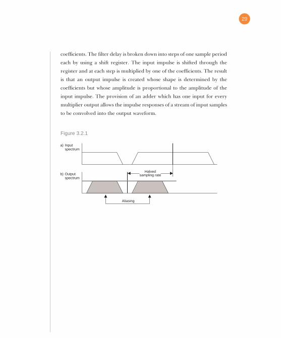
are halved. Fig.3.2.1a) shows the spectrum of a typical sampled system
where the sampling rate is a little more than twice the analog bandwidth.
Attempts to halve the sampling rate for downconversion by simply omitting
alternate samples, a process known as decimation, will result in aliasing, as
shown in b). It is intuitive that omitting every other sample is the same as
if the original sampling rate was halved. In any sampling rate conversion
system, in order to prevent aliasing, it is necessary to incorporate low-pass
filtering into the system where the cut-off frequency reflects the lower of
the two sampling rates concerned. Fig.3.2.2 shows an example of a low-
pass filter having an ideal rectangular frequency response. The Fourier
transform of a rectangle is a sinx/x curve which is the ideal impulse
response. The windowing process is omitted for clarity. The sinx/x curve is
sampled at the sampling rate in use in order to provide a series of
Frequency
Non-ideal response
Frequency
∞ Ideal frequencyresponse∞ Infinite
window
Finitewindow
28
coefficients. The filter delay is broken down into steps of one sample period
each by using a shift register. The input impulse is shifted through the
register and at each step is multiplied by one of the coefficients. The result
is that an output impulse is created whose shape is determined by the
coefficients but whose amplitude is proportional to the amplitude of the
input impulse. The provision of an adder which has one input for every
multiplier output allows the impulse responses of a stream of input samples
to be convolved into the output waveform.
Figure 3.2.1
Halvedsampling rate
a) Inputspectrum
Aliasing
b) Outputspectrum
29

Figure 3.2.2
Once the low pass filtering step is performed, the base bandwidth has been
halved, and then half the sampling rate will suffice. Alternate samples can
be discarded to achieve this.
There are various ways in which such a filter can be implemented.
Hardware may be configured as shown, or in a number of alternative
arrangements which give the same results. The filtering process may be
performed algorithmically in a processor which is programd to multiply
and accumulate. In practice it is not necessary to compute the values of
samples which will be discarded. The filter only computes samples which
will be retained, consequently only one output computation is made for
every two input sample shifts.
DelaysIn
Impulse response(sinx/x)
Output Impulseetc.etc.
Coefficients
Multiply bycoefficients
OutAdders
30

3.3 Upconversion
Following a compression codec in which pre-filtering has been used, it is
generally necessary to return the sampling rate to some standard value.
For example, 4:1:1 video would need to be upconverted to 4:2:2 format
before it could be output as a standard SDI (serial digital interface) signal.
Upconversion requires interpolation. Interpolation is the process of
computing the value of a sample or samples which lie off the sampling
matrix of the source signal. It is not immediately obvious how interpolation
works as the input samples appear to be points with nothing between them.
One way of considering interpolation is to treat it as a digital simulation of
a digital to analog conversion. According to sampling theory, all sampled
systems have finite bandwidth. An individual digital sample value is
obtained by sampling the instantaneous voltage of the original analog
waveform, and because it has zero duration, it must contain an infinite
spectrum. However, such a sample can never be seen or heard in that form
because the spectrum of the impulse is limited to half of the sampling rate
in a reconstruction or anti-image filter. The impulse response of an ideal
filter converts each infinitely short digital sample into a sinx/x pulse whose
central peak width is determined by the response of the reconstruction
filter, and whose amplitude is proportional to the sample value. This
implies that, in reality, one sample value has meaning over a considerable
timespan, rather than just at the sample instant. A single pixel has meaning
over the two dimensions of a frame and along the time axis. If this were not
true, it would be impossible to build a DAC let alone an interpolator.
If the cut-off frequency of the filter is one-half of the sampling rate, the
impulse response passes through zero at the sites of all other samples. It
can be seen from Fig.3.3.1 that at the output of such a filter, the voltage at
the centre of a sample is due to that sample alone, since the value of all
other samples is zero at that instant. In other words the continuous time
output waveform must join up the tops of the input samples. In between
31

the sample instants, the output of the filter is the sum of the contributions
from many impulses, and the waveform smoothly joins the tops of the
samples. If the waveform domain is being considered, the anti-image filter
of the frequency domain can equally well be called the reconstruction filter.
It is a consequence of the band-limiting of the original anti-aliasing filter
that the filtered analog waveform could only travel between the sample
points in one way. As the reconstruction filter has the same frequency
response, the reconstructed output waveform must be identical to the
original band-limited waveform prior to sampling.
Figure 3.3.1
4:1:1 to 4:2:2 conversion requires the colour difference sampling rate to be
exactly doubled. Fig.3.3.2 shows that half of the output samples are
identical to the input, and new samples need to be computed half way
between them. The ideal impulse response required will be a sinx/x curve
which passes through zero at all adjacent input samples. Fig.3.3.3 shows
that this impulse response can be re-sampled at half the usual sample
spacing in order to compute coefficients which the express the same
impulse at half the previous sample spacing. In other words, if the height
of the impulse is known, its value half a sample away can be computed. If
a single input sample is multiplied by each of these coefficients in turn, the
Sinx/x impulsesdue to sample
Analogue outputSample
etc. etc.
32

impulse response of that sample at the new sampling rate will be obtained.
Note that every other coefficient is zero, which confirms that no
computation is necessary on the existing samples; they are just transferred
to the output. The intermediate sample is computed by adding together
the impulse responses of every input sample in the window. Fig.3.3.4
shows how this mechanism operates.
Figure 3.3.2
Figure 3.3.3
Analogue waveformresulting from low-passfiltering of input samples
Position of adjacent input samples
0.127 -0.21 0.64 0.64 -0.21 0.127
Input samples
Output samples
33

Figure 3.3.4
Input samples
-0.21 X AContribution fromsample A
Sample value A
Sample value B
C Sample value
D Sample value
0.64 X BContribution fromsample B
0.64 X CContribution fromsample C
-0.21 X DContribution fromsample D
A B C D
Interpolated sample value= -0.21A + 0.64B + 0.64C - 0.21D
34

3.4 Transforms
In many types of video compression advantage is taken of the fact that a
large signal level will not be present at all frequencies simultaneously. In
audio compression a frequency analysis of the input signal will be needed
in order to create a masking model. Frequency transforms are generally
used for these tasks. Transforms are also used in the phase correlation
technique for motion estimation.
3.5 The Fourier transform
The Fourier transform is a processing technique which analyses signals
changing with respect to time and expresses them in the form of a
spectrum. Any waveform can be broken down into frequency components.
Fig.3.5.1 shows that if the amplitude and phase of each frequency
component is known, linearly adding the resultant components results in
the original waveform. This is known as an inverse transform.
35
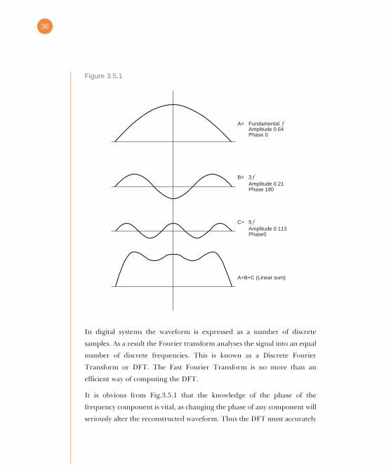
Figure 3.5.1
In digital systems the waveform is expressed as a number of discrete
samples. As a result the Fourier transform analyses the signal into an equal
number of discrete frequencies. This is known as a Discrete Fourier
Transform or DFT. The Fast Fourier Transform is no more than an
efficient way of computing the DFT.
It is obvious from Fig.3.5.1 that the knowledge of the phase of the
frequency component is vital, as changing the phase of any component will
seriously alter the reconstructed waveform. Thus the DFT must accurately
A= FundamentalAmplitude 0.64Phase 0
B= 3Amplitude 0.21Phase 180
C= 5Amplitude 0.113Phase0
A+B+C (Linear sum)
36
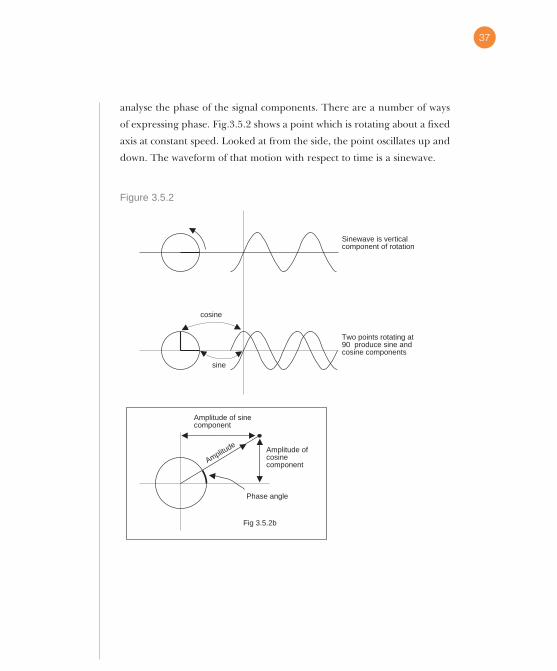
analyse the phase of the signal components. There are a number of ways
of expressing phase. Fig.3.5.2 shows a point which is rotating about a fixed
axis at constant speed. Looked at from the side, the point oscillates up and
down. The waveform of that motion with respect to time is a sinewave.
Figure 3.5.2
Sinewave is verticalcomponent of rotation
Amplitude of sinecomponent
sine
Two points rotating at90 produce sine andcosine components
cosine
Amplitude ofcosinecomponentAmplitu
de
Fig 3.5.2b
Phase angle
37

One way of defining the phase of a waveform is to specify the angle
through which the point has rotated at time zero (T=0). If a second point
is made to revolve at 90 degrees to the first, it would produce a cosine wave
when translated. It is possible to produce a waveform having arbitrary
phase by adding together the sine and cosine wave in various proportions
and polarities. For example adding the sine and cosine waves in equal
proportion results in a waveform lagging the sine wave by 45 degrees.
Fig.3.5.2b also shows that the proportions necessary are respectively the
sine and the cosine of the phase angle. Thus the two methods of describing
phase can be readily interchanged.
The Fourier transform spectrum-analyses a block of samples by searching
separately for each discrete target frequency. It does this by multiplying
the input waveform by a sine wave having the target frequency and adding
up or integrating the products. Fig.3.5.3a) shows that multiplying by the
target frequency gives a large integral when the input frequency is the
same, whereas Fig.3.5.3b) shows that with a different input frequency (in
fact all other different frequencies) the integral is zero showing that no
component of the target frequency exists. Thus a from a real waveform
containing many frequencies all frequencies except the target frequency
are excluded.
38

Figure 3.5.3
Fig.3.5.3c) shows that the target frequency will not be detected if it is phase
shifted 90 degrees as the product of quadrature waveforms is always zero.
Thus the Fourier transform must make a further search for the target
frequency using a cosine wave. It follows from the arguments above that
the relative proportions of the sine and cosine integrals reveals the phase
Input waveform
Integral of product
Targetfrequency
Input waveform
Targetfrequency
Integral = 0
Input waveform
Targetfrequency
Integral = 0
Product
Product
Product
a)
b)
c)
39

of the input component. For each discrete frequency in the spectrum there
must be a pair of quadrature searches.
The above approach will result in a DFT, but only after considerable
computation. However, a lot of the calculations are repeated many times
over in different searches. The FFT aims to give the same result with less
computation by logically gathering together all of the places where the
same calculation is needed and making the calculation once.
The amount of computation can be reduced by performing the sine and
cosine component searches together. Another saving is obtained by noting
that every 180 degrees the sine and cosine have the same magnitude but
are simply inverted in sign. Instead of performing four multiplications on
two samples 180 degrees apart and adding the pairs of products it is more
economical to subtract the sample values and multiply twice, once by a sine
value and once by a cosine value.
As a result of the FFT, the sine and cosine components of each frequency
are available. For use with phase correlation it is necessary to convert to the
alternative means of expression, i.e. phase and amplitude.
The number of frequency coefficients resulting from a DFT is equal to the
number of input samples. If the input consists of a larger number of
samples it must cover a larger area of the screen in video, a longer
timespan in audio, but its spectrum will be known more finely. Thus a
fundamental characteristic of transforms is that the more accurately the
frequency and phase of a waveform is analysed, the less is known about
where such frequencies exist.
3.6 The Discrete Cosine Transform
The two components of the Fourier transform can cause extra complexity
and for some purposes a single component transform is easier to handle.
The DCT (discrete cosine transform) is such a technique. Fig.3.6.1 shows
40
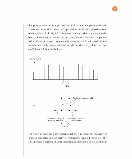
that prior to the transform process the block of input samples is mirrored.
Mirroring means that a reversed copy of the sample block placed in front
of the original block. Fig.3.6.1 also shows that any cosine component in the
block will continue across the mirror point, whereas any sine component
will suffer an inversion. Consequently when the whole mirrored block is
transformed, only cosine coefficients will be detected; all of the sine
coefficients will be cancelled out.
Figure 3.6.1
For video processing, a two-dimensional DCT is required. An array of
pixels is converted into an array of coefficients. Fig.3.6.2 shows how the
DCT process is performed. In the resulting coefficient block, the coefficient
Sine components ofinput samples
Sine components ofmirrored samples
b)
a)
Cosine components add
Cancel
Mirror
41

in the top left corner represents the DC component or average brightness
of the pixel block. Moving to the right the coefficients represent increasing
horizontal spatial frequency. Moving down, the coefficients represent
increasing vertical spatial frequency. The coefficient in the bottom right
hand corner represents the highest diagonal frequency.
Figure 3.6.2
3.7 Motion estimation
Motion estimation is an essential component of inter-field video
compression techniques such as MPEG. There are two techniques which
can be used for motion estimation in compression: block matching, the
most common method, and phase correlation.
Block matching is the simplest technique to follow. In a given picture, a
block of pixels is selected and stored as a reference. If the selected block is
part of a moving object, a similar block of pixels will exist in the next
picture, but not in the same place. Block matching simply moves the
reference block around over the second picture looking for matching pixel
Vertical
frequency
Vertical
distance
Horizontaldistance
Horizontalfrequency
DCT
IDCT
8x8 Pixel block 8x8 Coefficient block
42

values. When a match is found, the displacement needed to obtain it is the
required motion vector.
Whilst it is a simple idea, block matching requires an enormous amount of
computation because every possible motion must be tested over the
assumed range. Thus if the object is assumed to have moved over a sixteen
pixel range, then it will be necessary to test 16 different horizontal
displacements in each of sixteen vertical positions; in excess of 65,000
positions. At each position every pixel in the block must be compared with
the corresponding pixel in the second picture.
One way of reducing the amount of computation is to perform the
matching in stages where the first stage is inaccurate but covers a large
motion range whereas the last stage is accurate but covers a small range.
The first matching stage is performed on a heavily filtered and subsampled
picture, which contains far fewer pixels. When a match is found, the
displacement is used as a basis for a second stage which is performed with
a less heavily filtered picture. Eventually the last stage takes place to any
desired accuracy.
Inaccuracies in motion estimation are not a major problem in compression
because they are inside the error loop and are cancelled by sending
appropriate picture difference data. However, a serious error will result in
small correlation between the two pictures and the amount of difference
data will increase. Consequently quality will only be lost if that extra
difference data cannot be transmitted due to a tight bit budget.
Phase correlation works by performing a Fourier transform on picture
blocks in two successive pictures and then subtracting all of the phases of
the spectral components. The phase differences are then subject to a
reverse transform which directly reveals peaks whose positions correspond
to motions between the fields. The nature of the transform domain means
that if the distance and direction of the motion is measured accurately, the
43

area of the screen in which it took place is not. Thus in practical systems
the phase correlation stage is followed by a matching stage not dissimilar to
the block matching process. However, the matching process is steered by
the motions from the phase correlation, and so there is no need to attempt
to match at all possible motions. By attempting matching on measured
motion only the overall process is made much more efficient. One way of
considering phase correlation is that by using the Fourier transform to
break the picture into its constituent spatial frequencies the hierarchical
structure of block matching at various resolutions is in fact performed in
parallel.
The details of the Fourier transform are described in section 3.5. A one
dimensional example will be given here by way of introduction. A row of
luminance pixels describes brightness with respect to distance across the
screen. The Fourier transform converts this function into a spectrum of
spatial frequencies (units of cycles per picture width) and phases.
All television signals must be handled in linear-phase systems. A linear
phase system is one in which the delay experienced is the same for all
frequencies. If video signals pass through a device which does not exhibit
linear phase, the various frequency components of edges become displaced
across the screen. Fig.3.7.1 shows what phase linearity means. If the left
hand end of the frequency axis (zero) is considered to be firmly anchored,
but the right hand end can be rotated to represent a change of position
across the screen, it will be seen that as the axis twists evenly the result is
phase shift proportional to frequency. A system having this characteristic is
said to have linear phase.
44
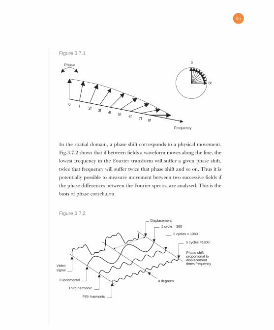
Figure 3.7.1
In the spatial domain, a phase shift corresponds to a physical movement.
Fig.3.7.2 shows that if between fields a waveform moves along the line, the
lowest frequency in the Fourier transform will suffer a given phase shift,
twice that frequency will suffer twice that phase shift and so on. Thus it is
potentially possible to measure movement between two successive fields if
the phase differences between the Fourier spectra are analysed. This is the
basis of phase correlation.
Figure 3.7.2
0 degrees
Videosignal
Displacement
Fundamental
Fifth harmonic
Third harmonic
1 cycle = 360
3 cycles = 1080
5 cycles =1800
Phase shiftproportional todisplacementtimes frequency
Frequency
Phase0
8f
0 f 2f 3f5f 6f 7f 8f
4f
45
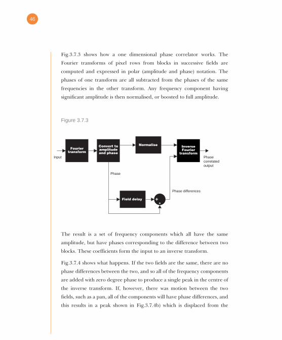
Fig.3.7.3 shows how a one dimensional phase correlator works. The
Fourier transforms of pixel rows from blocks in successive fields are
computed and expressed in polar (amplitude and phase) notation. The
phases of one transform are all subtracted from the phases of the same
frequencies in the other transform. Any frequency component having
significant amplitude is then normalised, or boosted to full amplitude.
Figure 3.7.3
The result is a set of frequency components which all have the same
amplitude, but have phases corresponding to the difference between two
blocks. These coefficients form the input to an inverse transform.
Fig.3.7.4 shows what happens. If the two fields are the same, there are no
phase differences between the two, and so all of the frequency components
are added with zero degree phase to produce a single peak in the centre of
the inverse transform. If, however, there was motion between the two
fields, such as a pan, all of the components will have phase differences, and
this results in a peak shown in Fig.3.7.4b) which is displaced from the
Phasecorrelatedoutput
Normalise InverseFourier
transformInput
Convert toamplitudeand phase
Field delay
Phase differences
Phase
Fouriertransform
46

centre of the inverse transform by the distance moved. Phase correlation
thus actually measures the movement between fields.
Figure 3.7.4
First image
Inversetransform
2nd Image
Central peak= no motion
Peak displacementmeasures motion
a) b)
c)
Peak indicatesobject moving
to left
0Peak indicatesobject movingto right
47

In the case where the line of video in question intersects objects moving at
different speeds, Fig.3.7.4c) shows that the inverse transform would
contain one peak corresponding to the distance moved by each object.
Whilst this explanation has used one dimension for simplicity, in practice
the entire process is two dimensional. A two dimensional Fourier transform
of each field is computed, the phases are subtracted, and an inverse two
dimensional transform is computed, the output of which is a flat plane out
of which three dimensional peaks rise. This is known as a correlation
surface.
Fig.3.7.5 shows some examples of a correlation surface. At a) there has
been no motion between fields and so there is a single central peak. At b)
there has been a pan and the peak moves across the surface. At c) the
camera has been depressed and the peak moves upwards. Where more
complex motions are involved, perhaps with several objects moving in
different directions and/or at different speeds, one peak will appear in the
correlation surface for each object. It is a fundamental strength of phase
correlation that it actually measures the direction and speed of moving
objects rather than estimating, extrapolating or searching for them.
48

Figure 3.7.5
However it should be understood that accuracy in the transform domain is
incompatible with accuracy in the spatial domain. Although phase
correlation accurately measures motion speeds and directions, it cannot
specify where in the picture these motions are taking place. It is necessary
to look for them in a further matching process. The efficiency of this
process is dramatically improved by the inputs from the phase correlation
stage.
49
Section 4 - Audio compressionIn this section we look at the principles of audio compression which will
serve as an introduction to the description of MPEG in section 6.
4.1 When to compress audio
The audio component of uncompressed television only requires about one
percent of the overall bit rate. In addition human hearing is very sensitive
to audio distortion, including that caused by clumsy compression.
Consequently for many television applications, the audio need not be
compressed at all. For example, compressing video by a factor of two
means that uncompressed audio now represents two percent of the bit rate.
Compressing the audio is simply not worthwhile in this case. However, if
the video has been compressed by a factor of fifty, then the audio and video
bit rates will be comparable and compression of the audio will then be
worthwhile.
4.2 The basic mechanisms
All audio data reduction relies on an understanding of the hearing
mechanism and so is a form of perceptual coding. The ear is only able to
extract a certain proportion of the information in a given sound. This
could be called the perceptual entropy, and all additional sound is
redundant. Section 1 introduced the concept of auditory masking which is
the inability of the ear to detect certain sounds in the presence of others.
The main techniques used in audio compression are:
* Requantizing and gain ranging
These are complementary techniques which can be used to reduce the
wordlength of samples, conserving bits. Gain ranging boosts low-level
signals as far above the noise floor as possible. Requantizing removes low
50

order bits, raising the noise floor. Using masking, the noise floor of the
audio can be raised, yet remain inaudible. The gain ranging must be
reversed at the decoder
* Predictive coding
This uses a knowledge of previous samples to predict the value of the next.
It is then only necessary to send the difference between the prediction and
the actual value. The receiver contains an identical predictor to which the
transmitted difference is added to give the original value.
* Sub band coding.
This technique splits the audio spectrum up into many different frequency
bands to exploit the fact that most bands will contain lower level signals
than the loudest one.
* Spectral coding.
A transform of the waveform is computed periodically. Since the transform
of an audio signal changes slowly, it need be sent much less often than
audio samples. The receiver performs an inverse transform. The transform
may be Fourier, Discrete Cosine (DCT) or Wavelet.
Most practical compression units use some combination of sub-band or
spectral coding and rely on masking the noise due to re-quantizing or
wordlength reduction of sub-band samples or transform coefficients.
4.3 Sub-band coding
Sub-band compression uses the fact that real sounds do not have uniform
spectral energy. When a signal with an uneven spectrum is conveyed by
PCM, the whole dynamic range is occupied only by the loudest spectral
component, and all other bands are coded with excessive headroom. In its
simplest form, sub-band coding works by splitting the audio signal into a
number of frequency bands and companding each band according to its
51

own level. Bands in which there is little energy result in small amplitudes
which can be transmitted with short wordlength. Thus each band results in
variable length samples, but the sum of all the sample wordlengths is less
than that of PCM and so a coding gain can be obtained.
The number of sub-bands to be used depends upon what other technique
is to be combined with the sub-band coding. If used with requantizing
relying on auditory masking, the sub-bands should be narrower than the
critical bands of the ear, and therefore a large number will be required,
ISO/MPEG Layers 1 and 2, for example, use 32 sub-bands. Fig.4.3.1 shows
the critical condition where the masking tone is at the top edge of the sub
band. Obviously the narrower the sub band, the higher the noise that can
be masked.
Figure 4.3.1
The band splitting process is complex and requires a lot of computation.
One bandsplitting method which is useful is quadrature mirror filtering.
The QMF is a kind of double filter which converts a PCM sample stream
Max. noiselevel
Sub band
Maskingthreshhold
Masking tone
52

into to two sample streams of half the input sampling rate, so that the
output data rate equals the input data rate. The frequencies in the lower
half of the audio spectrum are carried in one sample stream, and the
frequencies in the upper half of the spectrum are heterodyned or aliased
into the other. These filters can be cascaded to produce as many equal
bands as required.
Fig.4.3.2 shows the block diagram of a simple sub band coder. At the input,
the frequency range is split into sub bands by a filter bank such as a
quadrature mirror filter. The decomposed sub band data are then
assembled into blocks of fixed size, prior to reduction. Whilst all sub bands
may use blocks of the same length, some coders may use blocks which get
longer as the sub band frequency becomes lower. Sub band blocks are also
referred to as frequency bins.
53
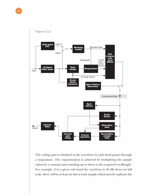
Figure 4.3.2
The coding gain is obtained as the waveform in each band passes through
a requantizer. The requantization is achieved by multiplying the sample
values by a constant and rounding up or down to the required wordlength.
For example, if in a given sub band the waveform is 36 dB down on full
scale, there will be at least six bits in each sample which merely replicate the
MVX(compress
scale factor
MPEG2)
1024 pointFFT
32 BandFilter bank
Input
Maskingmodel
RequantizerGain
ranger
Scalefactor
measure Sync PatternGenerator
Scalefactor
Allocationdata
Deserialisesample
data
Syncdetect
Compressed data
Inversequantize
Inversegain
range
Inversefilter
Output
Layer 2
Layer 1
Wordlength
Allocation data
Variablelengthsampledata bins
32 Scale factors
54

sign bit. Multiplying by 64 will bring the high order bits of the sample into
use, allowing bits to be lost at the lower end by rounding to a shorter
wordlength. The shorter the wordlength, the greater the coding gain, but
the coarser the quantisation steps and therefore the level of quantisation
error. If a fixed data reduction factor is employed, the size of the coded
output block will be fixed. The requantization wordlengths will have to be
such that the sum of the bits from each sub band equals the size of the
coded block. Thus some sub bands can have long wordlength coding if
others have short wordlength coding. The process of determining the
requantization step size, and hence the wordlength in each sub band, is
known as bit allocation. The bit allocation may be performed by analysing
the power in each sub band, or by a side chain which performs a spectral
analysis or transform of the audio. The complexity of the bit allocation
depends upon the degree of compression required. The spectral content is
compared with an auditory masking model to determine the degree of
masking which is taking place in certain bands as a result of higher levels
in other bands. Where masking takes place, the signal is quantized more
coarsely until the quantizing noise is raised to just below the masking level.
The coarse quantisation requires shorter wordlengths and allows a coding
gain. The bit allocation may be iterative as adjustments are made to obtain
the best masking effect within the allowable data rate.
The samples of differing wordlength in each bin are then assembled into
the output coded block. The frame begins with a sync pattern to reset the
phase of deserialisation, and a header which describes the sampling rate
and any use of pre-emphasis. Following this is a block of 32 four-bit
allocation codes. These specify the wordlength used in each sub band and
allow the decoder to deserialize the sub band sample block. This is followed
by a block of 32 six-bit scale factor indices, which specify the gain given to
each band during normalisation. The last block contains 32 sets of 12
samples. These samples vary in wordlength from one block to the next,
55
and can be from 0 to 15 bits long. The deserializer has to use the 32
allocation information codes to work out how to deserialize the sample
block into individual samples of variable length. Once all of the samples are
back in their respective frequency bins, the level of each bin is returned to
the original value. This is achieved by reversing the gain increase which
was applied before the requantizer in the coder. The degree of gain
reduction to use in each bin comes from the scale factors. The sub bands
can then be recombined into a continuous audio spectrum in the output
filter which produces conventional PCM of the original wordlength.
The degree of compression is determined by the bit allocation system. It is
not difficult to change the output block size parameter to obtain a different
compression factor. The bit allocator simply iterates until the new block
size is filled. Similarly the decoder need only deserialize the larger block
correctly into coded samples and then the expansion process is identical
except for the fact that expanded words contain less noise. Thus codecs
with varying degrees of compression are available which can perform
different bandwidth/performance tasks with the same hardware.
4.4 Transform coding
Fourier analysis allows any periodic waveform to be represented by a set of
harmonically related components of suitable amplitude and phase. The
transform of a typical audio waveform changes relatively slowly. The slow
growth of sound from an organ pipe or a violin string, or the slow decay of
most musical sounds allow the rate at which the transform is sampled to be
reduced, and a coding gain results. A further coding gain will be achieved
if the components which will experience masking are quantized more
coarsely.
Practical transforms require blocks of samples rather than an endless
stream. One solution is to cut the waveform into short overlapping
segments or windows and then to transform each individually as shown in
56

Fig.4.4.1. Thus every input sample appears in just two transforms, but with
variable weighting depending upon its position along the time axis.
Figure 4.4.1
The DFT (discrete Fourier transform) requires intensive computation,
owing to the requirement to use complex arithmetic to render the phase of
the components as well as the amplitude. An alternative is to use Discrete
Cosine Transforms (DCT) in which the coefficients are single numbers. In
any transform, accuracy of frequency resolution is obtained with the
penalty of poor time resolution, giving a problem locating transients
properly on the time axis. The wavelet transform is especially good for
audio because its time resolution increases automatically with frequency.
The wordlength reduction or requantizing in the coder raises the
quantizing noise in the frequency band, but it does so over the entire
duration of the window. Fig.4.4.2 shows that if a transient occurs towards
the end of a window, the decoder will reproduce the waveform correctly,
but the quantizing noise will start at the beginning of the window and may
result in a pre-echo where a burst of noise is audible before the transient.
EncoderTime
57

Figure 4.4.2
One solution is to use a variable time window according to the transient
content of the audio waveform. When musical transients occur, short
blocks are necessary and the frequency resolution and hence the coding
gain will be low. At other times the blocks become longer and the frequency
resolution of the transform rises, allowing a greater coding gain.
4.5 Audio compression in MPEG
The layers and levels of MPEG audio coding are shown in Fig.4.5.1. In
MPEG-1 audio inputs have sampling rates of 32, 44.1 or 48KHz. There are
three coding algorithms of ascending complexity, known as Layers 1,2 and
3. There are four operating modes in MPEG-1 which are shown in
Fig.4.5.2. In mono mode, only one audio signal is handled. In stereo
mode, two audio signals are handled, but the data are held in a common
buffer so that entropy variations between the two channels can be
exploited. In dual mono mode, the available bit rate is exactly halved so
that two independent unrelated audio signals, perhaps a dual language
soundtrack, can be handled. In joint stereo mode, only the lower half of
Input level
Masked
Noisefloor
Coding block
Transient
Pre-noisenot masked
Time
58
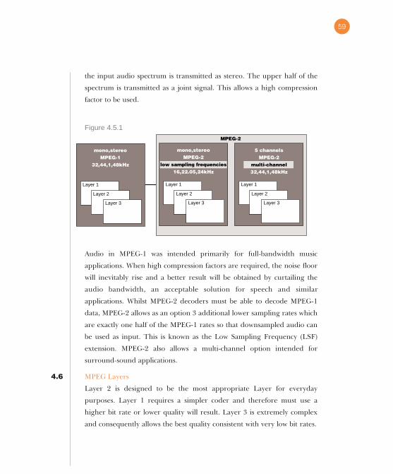
the input audio spectrum is transmitted as stereo. The upper half of the
spectrum is transmitted as a joint signal. This allows a high compression
factor to be used.
Figure 4.5.1
Audio in MPEG-1 was intended primarily for full-bandwidth music
applications. When high compression factors are required, the noise floor
will inevitably rise and a better result will be obtained by curtailing the
audio bandwidth, an acceptable solution for speech and similar
applications. Whilst MPEG-2 decoders must be able to decode MPEG-1
data, MPEG-2 allows as an option 3 additional lower sampling rates which
are exactly one half of the MPEG-1 rates so that downsampled audio can
be used as input. This is known as the Low Sampling Frequency (LSF)
extension. MPEG-2 also allows a multi-channel option intended for
surround-sound applications.
4.6 MPEG Layers
Layer 2 is designed to be the most appropriate Layer for everyday
purposes. Layer 1 requires a simpler coder and therefore must use a
higher bit rate or lower quality will result. Layer 3 is extremely complex
and consequently allows the best quality consistent with very low bit rates.
mono,stereoMPEG-1
32,44,1,48kHz
Layer 1
Layer 2
Layer 3
mono,stereoMPEG-2
low sampling frequencies16,22.05,24kHz
Layer 1
Layer 2
Layer 3
5 channelsMPEG-2
multi-channel32,44,1,48kHz
Layer 1
Layer 2
Layer 3
MPEG-2
59

Layer 1 uses a sub-band coding scheme having 32 equal bands and works
as described in section 4.3. The auditory model is obtained from the levels
in the sub-bands themselves so no separate spectral analysis is needed.
Layer 2 uses the same sub-band filter, but has a separate Transform
analyser which creates a more accurate auditory model. In Level 2 the
processing of the scale factors is more complex, taking advantage of
similarity in scale factors from one frame to the next to reduce the amount
of scale data transmitted. Layers 1 and 2 have a constant frame length of
1152 audio samples.
Layer 3 is much more complex because it attempts a very accurate auditory
modelling process. A 576-line Discrete Cosine Transform is calculated, and
various numbers of lines are grouped together to simulate the varying width
of the critical bands of human hearing. The audio is transmitted as transform
coefficients which have been requantized according to the masking model.
Huffman coding is used to lower the data rate further. The decoder requires
an inverse transform process. Layer 3 also supports a variable frame length
which allows entropy variations in the audio input to be better absorbed.
Layer 3 supports additional modes than the four modes of Layers 1 and 2.
These are shown in Fig.4.5.2. M-S coding produces sum and difference
60
MonoStereoDual MonoJoint Stereo
M-S StereoIntensity StereoIntensity & M-S Stereo
All layers
Layer3
only
signals from the L-R stereo. The S or difference signal will have low
entropy when there is correlation between the two input channels. This
allows a further saving of bit rate.
Intensity coding is a system where in the upper part of the audio frequency
band, for each scale factor band only one signal is transmitted, along with
a code specifying where in the stereo image it belongs. The decoder has the
equivalent of a pan-pot so that it can output the decoded waveform of each
band at the appropriate level in each channel. The lower part of the audio
band may be sent as L-R or as M-S.
61
Section 5 - Video compressionIn this section the essential steps used in video compression will be
detailed. This will form an introduction to the description of MPEG in
section 6.
5.1 Spatial and temporal redundancy
Video compression requires the identification of redundancy in typical
source material. There are two basic forms of redundancy which can be
exploited. The first of these is intra-frame or spatial redundancy, which is
redundancy that can be identified in a single image without reference to
any other. The second is inter-frame or temporal redundancy which can
be identified from one frame to the next.
5.2 The Discrete Cosine Transform
Spatial redundancy is found in all real program material. Where a sizeable
object is recognisable in the picture, all of the pixels representing that
object will have quite similar values. Large objects produce low spatial
frequencies, whereas small objects produce high spatial frequencies.
Generally these frequencies will not be present at high level at the same
time. Normal PCM video has to be able to transmit the whole range of
spatial frequencies, but if a frequency analysis is performed, only those
frequencies actually present need be transmitted. Consequently a major
step in intra-coding is to perform a spatial frequency analysis of the image.
In MPEG the Discrete Cosine Transform or DCT (see section 3) is used.
Fig.5.2.1 shows how the two-dimensional DCT works. The image is
converted a block at a time. A typical block is 8 x 8 pixels. The DCT
converts the block into a block of 64 coefficients. A coefficient is a number
which describes the amount of a particular spatial frequency which is
present. In the figure the pixel blocks which result from each coefficient
62

are shown. The top left coefficient represents the average brightness of the
block and so is the arithmetic mean of all the pixels or the DC component.
Going across to the right, the coefficients represent increasing horizontal
spatial frequency. Going downwards the coefficients represent increasing
vertical spatial frequency.
Figure 5.2.1
Now the DCT itself doesn’t achieve any compression. In fact the
wordlength of the coefficients will be longer than that of the source pixels.
What the DCT does is to convert the source pixels into a form in which
redundancy can be identified. As not all spatial frequencies are
simultaneously present, the DCT will output a set of coefficients where
some will have substantial values, but many will have values which are
63
almost or actually zero. Clearly if a coefficient is zero it makes no difference
whether it’s sent or not. If a coefficient is almost zero, omitting it would
have the same effect as adding the same spatial frequency to the image but
in the opposite phase. The decision to omit a coefficient is based on how
visible that small unwanted signal would be. If a coefficient is too large to
omit, compression can also be achieved by reducing the number of bits
used to carry the coefficient. This has the same effect; a small noise is added
to the picture.
5.3 Weighting
Visibility of spatial frequencies by the human viewer is not uniform; much
higher levels of noise can be tolerated at high frequencies. Consequently
weighting is used so that any noise which is created is concentrated at high
frequencies. Coefficients are divided by a weighting factor which is a
function of the position in the block. The DC component is unweighted
whereas the division factor increases towards the bottom right hand
corner. At the decoder an inverse weighting process is needed. This
multiplies higher frequency coefficients by greater factors, raising the high
frequency noise.
After weighting, the value of certain coefficients will be even smaller. On
typical program material, large value coefficients are mostly found in the
top left corner, the remainder of the coefficients are often negligible or
zero. It is an advantage to transmit the coefficients in a zigzag sequence
starting from the top left corner. When this is done, the non-zero
coefficients are typically transmitted soonest, leaving typically zero
coefficients at the end. At some point when all subsequent coefficients are
zero, it is more efficient to terminate the transmission with a simple
character which tells the receiver that there are no more non-zero
coefficients.
64

5.4 Variable length coding
Analysis of typical source data shows that the probability of low value
coefficients having many leading zeros is higher than that of large value
coefficients sent as 4,2. Where the probability of such values is known it is
more efficient to use a coding scheme which takes advantage of such a
distribution.
The Huffman coding scheme allocates shorter codes to more probable
values and longer codes to values which are less probable. When used with
source data having assumed probability an improvement in transmission
efficieny is obtained.
In DCT coding it is often the case that may coefficients have a value of zero.
In this case run length coding simply tells the decoder how many zero
valued coefficients were present instead of sending each separately.
5.5 Intra-coding
Fig.5.5.1 shows a complete intra-coding scheme. The input picture is
converted from raster scan to blocks. The blocks are subject to a DCT. The
coefficients are then zigzag scanned and weighted, prior to being
requantized (wordlength shortening) and subject to run-length coding. In
practical systems a constant output bit rate is required even though the
source entropy varies. There are two solutions. One is to use a buffer to
absorb the variations. The other is to measure the quantity of output data
and compare it with the required amount. If there is too much data, the
requantizer is made to shorten the wordlength of the coefficients more
severely. If there is insufficient data the requantizing is eased.
65
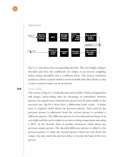
Figure 5.5.1
Fig.5.5.1. also shows the corresponding decoder. The run length coding is
decoded and then the coefficients are subject to an inverse weighting
before being assembled into a coefficient block. The inverse transform
produces a block of pixels which is stored in RAM with other blocks so that
a raster scanned output can be produced.
5.6 Inter-coding
The system of Fig.5.5.1 is basically that used in JPEG which is designed for
still images. Intra-coding takes no advantage of redundancy between
pictures. In typical source material one picture may be quite similar to the
previous one. Fig.5.6.1 shows how a differential coder works. A frame
store is required which delays the previous picture. Each pixel in the
previous picture is subtracted from the current picture to produce a
difference picture. The difference picture is a two-dimensional image in its
own right and this can be subject to an intra-coding compression step using
a DCT. At the decoder there is another framestore which delays the
previous output picture. The decoded difference picture is added to the
previous picture to make the current picture which not only forms the
output, but also enters the pircture delay to become the basis of the next
picture.
Rasterscan toblock
Video out
Video inDCT
WeightCoeffi-cients
Zig-zag
scan
Run lengthcode +buffer
Run lengthdecode +
buffer
Inverseweight
InverseDCT
Block to rasterscan
Channel
66

Figure 5.6.1
In differential coding it is important to prevent the build up of small errors
which might accumulate over a succession of pictures. One such source of
error is the compression of the difference picture. Fig.5.6.2 shows how this
error is removed. Both the encoder and the decoder contain an identical
difference picture decoder. When the encoder subtracts a previous picture
from a current picture, it actually subtracts a locally decoded compressed
picture identical to that which the real decoder will have. Consequently any
small errors due to the compression of earlier difference pictures are
removed.
Picturedelay
In
Differencepicture
67

Figure 5.6.2
5.7 Motion compensation
Differential coding works well on largely static picture material, but falls
down heavily when there is motion. In the extreme case of a pan, the value
of every pixel changes and the difference picture contains nearly as much
data as the original picture. However, a pan does not change many pixel
values at all, the values are just present in a different place. Consequently
motion compensation is required to obtain high compression factors in
differential coding schemes.
Compressdifference
picture
Picturedelay
Video out
Differencepicture
Channel
Video in
Decodedifference
pictureLocally decodedprevious picture
Difference picturewith compressionerror
Picturedelay
Decodedifference
picture
Decoder
Encoder
68
Fig.5.7.1 shows that in a motion compensated compressor, areas of two
successive pictures are compared in order to determine the direction and
distance of relative motion between the frames. These are expressed as a
two dimensional vector. The encoder uses the motion vector to shift pixels
from the previous picture to make what is called a predicted picture prior
to subtracting them from the current or actual picture. If the motion
measurement has been accurate, the shifting process will have aligned the
objects in the predicted frame with their position in the actual frame and
only a small amount of difference data will result. Clearly if the motion
vectors are transmitted along with the difference data, the decoder can
make the same shift of the previous frame to produce its own predicted
frame. Adding the difference data will produce the decoded current frame.
69

Figure 5.7.1
The picture is broken up into rectangular areas called macroblocks. Each
of these macroblocks has its own motion vector which applies to the whole
block. Clearly if the edge of a moving object lies across a macroblock, some
of the macroblock is moving and some is not. This situation may be
handled by setting the motion vectors to zero and handling the moving
part with difference data, or by using non-zero motion vectors and
handling the stationary part with difference data. A smart compressor
might try both to see which approach yielded the smaller bit rate.
As motion in real program material tends to be relatively constant across
several pictures, the motion vectors are transmitted differentially.
Consequently a motion vector parameter of zero is interpreted as the same
motion continuing. The vectors from the previous picture are copied. If
the motion slows down or changes direction, vector differences are sent.
Vectors
Pixeldi f ferencedata
Horizontalmot ion
Vert icalmot ion
A B
MotionEstimator
Measure mot ionbetween A+B
Use mot ion vectorto shi f t A
Subtract A f rom B
Transmit vectorsand di f ferencedata
70

5.8 I pictures
Pure differential coders cannot be used in practice because the decoder can
only make sense of the transmission if it is received from the beginning.
Any transmission errors will affect the picture indefinitely afterwards. In
practice differential transmission systems punctuate the difference pictures
with periodic absolute pictures which are intra-coded. Fig.5.8.1 shows the
principle. The intra-coded or I pictures are created by turning off the
prediction system so that no previous data are subtracted from the input.
The difference picture becomes an absolute picture. In between I pictures,
the motion compensated prediction process operates and P pictures,
consisting of motion vectors and DCT compressed difference values are
created.
Figure 5.8.1
In the case of film originated material which has been played on a telecine,
knowledge of the scanning process is useful to an encoder. For example a
60Hz telecine uses 3:2 pulldown to obtain 60 Hz field rate from 24 Hz film.
In the three field frame, the third field is a direct repeat of the first field
and consequently carries no information. Only the first two fields are
I P P P I P P P I
Whole picturetransmitted
Differencepicturetransmitted
71

transmitted by the coder. The decoder can repeat one of them to recreate
the 3:2 sequence.
In both 50Hz and 60 Hz telecine, there can be no motion between the
fields which come from the same film frame. Consequently there is no
point in measuring motion or transmitting motion vectors for the second
field.
There is no requirement for absolute regularity in the I pictures. Picture
types are labelled so the decoder can automatically handle whatever it
receives. Cut edits in the incoming material cause large difference data.
With a suitable pre-processor, a compressor can anticipate the arrival of a
cut in the source material and make it coincide with an I picture so that the
most effective use of the bit rate is made.
It should be clear that editing of the bitstream is likely to be problematical
in a differential coding scheme. If the bitstream is switched at an arbitrary
point the decoder will be unable to produce pictures until the next I
picture arrives. Consequently editing is restricted to switching at I pictures.
This will be too restricting for production purposes and where editing is
anticipated, the two fields of an interlaced frame can be compressed as one
I picture and one P picture. Editing to frame accuracy is then possible,
Clearly the compression factor which can be obtained will be relatively
poor because of the frequent I pictures. This is consistent with the cautions
expressed in Section 1.
72
Section 6 - MPEGIn this section all of the concepts introduced in earlier sections are tied
together in a description of MPEG. MPEG is not a compression scheme as
such, in fact it is hard to define MPEG in a single term. MPEG is essentially
a set of standard tools, or defined algorithms, which can be combined in a
variety of ways to make real compression equipment.
6.1 Applications of MPEG
Unusually, MPEG does not define how the encoder should carry out
compression. Instead MPEG defines precisely how a decoder should
attribute meaning to a variety of compressed bitstreams. MPEG does not
suggest how to transmit the bitstream, as this will depend on the
application. The reason for this approach is that it allows a great deal of
flexibility whilst retaining compatibility. The manufacturers can use
proprietary encoding algorithms yet produce a standard bitstream. As
algorithms improve with time, the signals will still be compatible with
existing decoders.
The uses of video compression go beyond the requirements of broadcast
television. Applications range from small moving images on personal
computers to large high definition displays. Picture quality requirements
range from relatively poor for security and videophone purposes through
CD-I to transparent quality. Sometimes the same transmission needs to be
decoded to different standards. For example, there is no point in decoding
a high definition signal for display on a 12 inch TV set. Different
applications can afford different investments in encoder and decoder
complexity. In addition to video, MPEG caters for associated compressed
audio and means to multiplex audio and video together in a way which
retains synchronisation.
73

6.2 Profiles and Levels
The wide range of performance and complexity required is handled by
subdividing MPEG into Profiles and then dividing each profile into Levels.
Fig.6.2.1 shows that a Profile is a technique whereas a level is a constraint
such as picture size or bit rate used with that technique. Fig.6.2.1 also
shows the Profiles available.
Figure 6.2.1
The Simple Profile, as its name suggests, allows minimal complexity at
encoder and decoder. Basically a simple profile system uses no more than
the I and P pictures described in section 5.
The Main Profile is designed to be suitable for a large proportion of uses
and has received a lot of attention. The Main Profile will be described in
detail later in this section.
The SNR Scaleable Profile is a system in which two separate data streams
are used to carry one video signal. Together, the two data streams can be
Levels
Profiles
Low levelup to 352x288pixels4 MBit/s max.
Main levelup to 720x576pixels15 MBit/s max.
High 1440 levelUp to 720x576pixels60 MBit/s max.
High levelUp to 1920x1152pixels80 MBit/s max.
Simple
Main
S.N.Rscaleable
Spatialscaleable
High
M.P.M.L.
74

decoded to produce a high quality picture with a high signal-to-noise
ratio. However, if one of the data streams is not received, the result is a
picture having the same spatial resolution but with a reduced signal-to-
noise ratio. Instead of producing one compressed bitstream, the coder is
designed to produce a two streams. One of these carries a noisy picture,
whereas the other carries a “helper” signal which when added to the first
signal eliminates the noise. An anticipated use of the technology in DVB
(digital video broadcasting) where transmitters would radiate an SNR
scaleable signal where the first bitstream is transmitted with more power.
Fixed receivers with good antennas could receive both bitstreams and
produce a quality picture. In the case of poor reception only the more
powerful signal would get through allowing a poorer picture in
preference to no picture at all.
The Spatial Scaleable Profile is a system in which more than one data
stream can be used to reproduce a picture of different resolution
depending on the display. One data stream is a low-resolution picture
which can be decoded alone for display on small portable sets. Other data
streams are “spatial helper” signals which when added to the first signal
serve to increase its resolution for use on large displays.
The High Profile is temporally scaleable, allowing a transmission which can
be decoded into two different frame rates according to the complexity of
the decoder.
Within the Profile structure, a number of levels are available as shown in
Fig.6.2.1. The levels differ primarily in the resolution available and the bit
rate required. The Main Level is appropriate for Standard Definition
Television (SDTV). Consequently the majority of broadcast and
production interest is in the MPML (Main Profile Main Level) subset of
MPEG.
In general, an MPEG decoder with a given Profile and Level must be
75
capable of decoding inputs corresponding to lower profiles and levels as
well. Thus a scaleable decoder would continue to operate if it received a
main level or a simple level input.
Most of the hierarchy of MPEG is based on 4:2:0 format video where the
colour difference signals are vertically subsampled. For broadcast
purposes, it is widely believed that 4:2:2 working is required and a separate
4:2:2 profile has been proposed which is not in the hierarchy.
6.3 MPEG-1 and MPEG-2
MPEG-1 was the first document to be published. This described standards
for low-bit rate coding up to 1.5 megabits/sec. Interlace was not supported
and the resolution was limited, allowing a maximum of 352 x 288 pixels.
Up to 192kbit/sec could be used for stereo audio. The bit rate was largely
determined by that of a standard Compact Disc so that it could be used for
A/V applications such as CD-I and CD-ROM.
Clearly the uses of MPEG-1 in broadcasting are extremely limited, and
MPEG-2 was designed to rectify the problem. MPEG-2 supports interlace
and codes SDTV at between 3 and 15 megabits/sec or HDTV at 15-30
megabits/sec. The audio capability is extended to support surround sound.
Because of the hierarchical structure of MPEG, an MPEG-2 decoder will be
able to decode MPEG-1 signals, but not vice versa.
6.4 Bi-directional coding
One of the most powerful features of MPEG is the concept of bi-directional
coding. Section 5 introduced the concept of motion compensated
prediction and P pictures which were decoded by using the previous
picture as a basis, shifted by motion vectors and corrected with difference
data. Bi-directional coding takes this idea a step forward by allowing
prediction of part of a picture from earlier or later pictures.
Fig.6.4.1 shows an example of a picture sequence used in MPEG. The
76

sequence begins with an I picture as an anchor, and this and all pictures
until the next I picture are called a Group of Pictures (GOP). Within the
GOP are a number of forward predicted or P pictures. The first P picture
is decoded using the I picture as a basis. The next and subsequent P
pictures are decoded using the previous P picture as a basis. The
remainder of the pictures in the GOP are B pictures. B pictures may be
decoded using data from I or P pictures immediately before or afterwards
or taking an average of the two. As the pictures are divided into
macroblocks, each macroblock may be forward or backward predicted.
Obviously backward prediction cannot be used if the decoder does not yet
have the frame being projected backwards. The solution is to send the
pictures in the wrong order. After the I picture, the first P picture is sent
next. Once the decoder has the I and P pictures, the B pictures in between
can be decoded by moving motion compensated data forwards or
backwards. Clearly a bi-directional system needs more memory at encoder
and decoder and causes a greater coding delay. The simple profile of
MPEG dispenses with B pictures to make a complexity saving, but will not
be able to achieve such good quality at a given bit rate.
Figure 6.4.1
I1 B1 B2 P1 B3 B4 P2 B5 B6 P3 B7 B8 I2
I1 P1 B1 B2 P2 B3 B4 P3 B5 B6 I2 B7 B8
G.O.P
Bidirectional coding
Transmissionorder
77

The use of bi-directional coding becomes clear upon considering the
boundaries of a moving object. At the leading edge of an object, the
background is being concealed, consequently less data are required in
future frames. Background data are already known at the decoder and
forward prediction is the most efficient. However, at the trailing edge the
background is being revealed and background data will not be available in
past frames. However, more of the background will be available in future
frames so it is more efficient to use data from a later frame and discard
some of it. In practice a coder may perform both forward and backward
codings but only send the one which results in the smallest difference data.
6.5 Data types
The result of an MPEG compression of a single video signal will be a
number of different data types as follows:
1/ The decoder must be told the profile, the level and the size of the image
in macroblocks, although this need not be sent very often.
2/ The sequence of I,P and B frames must be specified so that the decoder
knows how to interpret and reorder the transmitted picture data. The
sequence parameters consist of one value specifying the number of
pictures in the GOP and another specifying the spacing of P pictures.
3/ The time to which a picture relates is indicated by sending a form of time
code.
4/ The weighting used in the compression process is variable and it may be
necessary to send the weighting matrix values if a default value has not
been used.
5/ The data allowing three types of picture to be decoded.
6.6 MPEG bitstream structure
The structure of a single MPEG bitstream begins with a Video Sequence as
shown in Fig.6.6.1. A Video Sequence contains a number of GOPs. The
78

sequence header specifies the profile and level, the picture size and the
frame rate. Optionally the weighting matrices used in the coder are carried.
Figure 6.6.1
Within the VideoSequence a number of GOPs are sent sequentially. Each
GOP begins with a GOP header containing the time code stamp of the first
picture.
Within each GOP, the first picture is always an I picture, whereas
subsequent pictures could be P or B. The picture header contains a code
specifying the type of picture and its time location within the GOP. As
pictures are sent out of sequence for bi-directional coding the picture
header is an important step in getting the display order correct.
Each picture is divided in two dimensions into 8 x 8 pixel blocks. As the
chroma has been subsampled by a factor of two, for every four luminance
79
MPEG2 bitstream syntax (without extensions)
Video Sequence sequence_start_codesequence_headersequence_end_code
Sequence header sequence_headercodehorizontal size valuevertical size value
pel_aspect_ratioframe ratebit rate
vbv_buffer_sizeconstrained parameter flagIntra & Inter quantizer matrices
macroblock_stuffingmacroblock_escapemacroblock_address_incrmacroblock_typeframe/field motion typedct_typequantizer_scale_codeforward motion vectorsbackward_motion_vectorscoded_block_pattern
full_pel_backward_vectorbackward_f_code
vbv_delayfull_pel_forward_vectorforward_f_code
picture_start_codetemporal_referencepicture_coding_type
Picture
PicturePicture
Picture
group start_codetime_codeclosed_gap_broken_link
Group of picturesGroup of pictures
Group of pictures
MacroblockSlice slice_start_code quantizer_scale_code
Macroblock Macroblock
Blockdct_dc_size_lum/chromdct_dc_differentialFirst DCT coeffSubsequent DCT coeffsEnd of Block
MacroblockMacroblockMacroblockSlice
Block 3Y
Block 1Y
Block 2Y
Block 4Y
Block 5Cb
Block 6Cr
Block 3Y
Block 1Y
Block 2Y
Block 4Y
Block 5Cb
Block 6Cr
Block 3Y
Block 1Y
Block 2Y
Block 4Y
Block 5Cb
Block 6Cr
Block 3Y
Block 1Y
Block 2Y
Block 4Y
Block 5Cb
Block 6Cr

blocks there is only one R-Y block and one B-Y block. A set of four
luminance blocks in a square and the two corresponding colour difference
blocks is the picture area carried in a macroblock. A macroblock is the unit
of picture information to which one motion vector applies and so there will
be a two-dimensional vector sent in each macroblock, except in I pictures
where there are by definition no vectors. In P pictures the vectors are
forward only, whereas in B pictures it is necessary to specify whether the
vector is forward or backward or whether a combination of the two is used.
A row of macroblocks across the screen is called a slice. It is not essentialfor
a slice to extend across the full width of a screen, although the edge of the
picture myst conicide with the edge of a slice. In the case where the full
width of the screen is occupied by a slice in 601 luminance there are 720
pixels per line so there will be 45 macroblocks per slice as 45 x 16 = 720.
Each slice carries its own address in the picture for synchronising purposes.
A number of slices makes up a whole picture. For example in the Low
Profile picture there is a maximum of 288 lines. There would be 18 slices
in the picture as 18 x 16 = 288.
6.7 Systems layer
The structure described so far is known as an elementary stream as it
carries only one channel of video. Other elementary streams will carry the
associated audio. The next layer of coding concerns the multiplexing of the
video and audio of several programs. This is known as the Systems layer.
A Program Stream consists of the video and audio for one service having
one common clock. Program Streams have variable length data packets
which are relatively unprotected and so are only suitable for error free
transmission or recording systems.
A Transport Stream is an alternative to a Program Stream. This uses fixed
length packets with error correction. Fig.6.7.1 shows a Transport Stream
packet which consists of 187 bytes of data. Although not part of MPEG, it
80
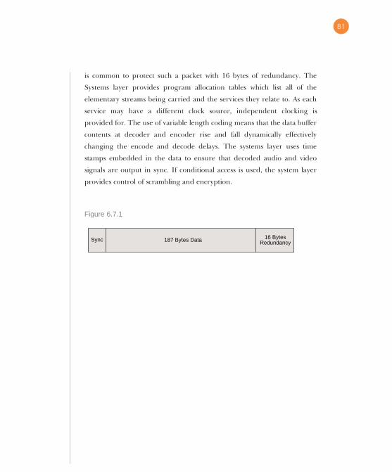
is common to protect such a packet with 16 bytes of redundancy. The
Systems layer provides program allocation tables which list all of the
elementary streams being carried and the services they relate to. As each
service may have a different clock source, independent clocking is
provided for. The use of variable length coding means that the data buffer
contents at decoder and encoder rise and fall dynamically effectively
changing the encode and decode delays. The systems layer uses time
stamps embedded in the data to ensure that decoded audio and video
signals are output in sync. If conditional access is used, the system layer
provides control of scrambling and encryption.
Figure 6.7.1
187 Bytes DataSync 16 BytesRedundancy
81


Compression is a technology which is important because it directly affects
the economics of many audio and video production and transmission
processes. The applications have increased recently with the availability of
international standards such as MPEG and supporting chip sets. In this
guide the subject is explained without unnecessary mathematics. In
addition to the theory, practical advice is given about getting the best out
of compression systems.
Other handbooks published by Snell & Wilcox include:
“The Engineers’ Guide to Standard Conversions” 1 900739 03 8
“The Engineers’ Guide to Decoding and Encoding” 1 900739 01 1
“The Engineers’ Guide to Motion Compensation” 1 900739 02 X
“Your Essential Guide to Digital” (NTSC) 1 900739 04 6
“Your Essential Guide to Digital” (PAL) 1 900739 05 4
Engineering with Vision £12.50/$20.00

85