Discussion Paper No. 2016-04

Matthias Dahm, PaulaGonzález & Nicolás Porteiro

April 2016

The Enforcement ofMandatory DisclosureRules

CeDEx Discussion Paper SeriesISSN 1749 - 3293

The Centre for Decision Research and Experimental Economics was founded in2000, and is based in the School of Economics at the University of Nottingham.

The focus for the Centre is research into individual and strategic decision-makingusing a combination of theoretical and experimental methods. On the theory side,members of the Centre investigate individual choice under uncertainty,cooperative and non-cooperative game theory, as well as theories of psychology,bounded rationality and evolutionary game theory. Members of the Centre haveapplied experimental methods in the fields of public economics, individual choiceunder risk and uncertainty, strategic interaction, and the performance of auctions,markets and other economic institutions. Much of the Centre's research involvescollaborative projects with researchers from other departments in the UK andoverseas.

Please visit http://www.nottingham.ac.uk/cedex for more information aboutthe Centre or contact

Suzanne RobeyCentre for Decision Research and Experimental EconomicsSchool of EconomicsUniversity of NottinghamUniversity ParkNottinghamNG7 2RDTel: +44 (0)115 95 14763Fax: +44 (0) 115 95 14159suzanne.robey@nottingham.ac.uk

The full list of CeDEx Discussion Papers is available at

http://www.nottingham.ac.uk/cedex/publications/discussion-papers/index.aspx

The Enforcement of Mandatory Disclosure Rules∗

Matthias Dahm†, Paula González‡and Nicolás Porteiro§

April 25, 2016

Abstract

This paper examines the incentives of a firm to invest in information about the qual-ity of its product and to disclose its findings. If the firm holds back information, it mightbe detected and fined. We show that optimal monitoring is determined by a trade-off.Stricter enforcement reduces the incentives for selective reporting but crowds out in-formation search. Our model implies that (i) the probability of detection and the finemight be complements; (ii) the optimal monitoring policy does not necessarily eliminateselective reporting entirely; (iii) even when there is some selective reporting in equilib-rium and more stringent monitoring is costless, increasing the probability of detectionmight not be beneficial; and (iv) when society values selectively reported information,the optimal fine might not be the largest possible fine.

Keywords: strategic information transmission, distrust effect, confidence effect, moni-toring, penalty, fine, sanction, detection probabilityJEL Classification No.: D82, L15

∗We would like to dedicate this paper to our co-author Nicolás Porteiro who passed away in April 2012.We are truly grateful for his friendship over many years and for all that we learned from him during that time.We are indebted to Inés Macho-Stadler, David Pérez-Castrillo and Daniel Seidmann for their careful reading ofthis paper. We are also grateful for valuable comments and suggestions from Helmut Bester, Farasat Bokhari,Subhasish M. Chowdhury, Thomas Gall, Paul Heidhues, Roberto Hernán-González, Sang-Hyun Kim, DavidMyatt, Pau Olivella, Carmelo Rodríguez-Álvarez, Marta Ronchetti, Roland Strausz, Marcos Vera-Hernándezand Ansgar Wohlschlegel. Financial support from Fundación Ramón Areces is gratefully acknowledged. Thiswork is partially supported by the research projects ECO2012-36480 and ECO2015-65408-R (Ministerio deCiencia y Tecnología) and FEDER. All errors are our sole responsibility.

†Corresponding author: University of Nottingham, School of Economics, University Park, Nottingham, NG72RD (UK); email: Matthias.Dahm@nottingham.ac.uk.

‡Universidad Pablo de Olavide, Department of Economics; email: pgonzalez@upo.es.§Universidad Pablo de Olavide, Department of Economics.

1 Introduction

In September 2004, the pharmaceutical company Merck voluntarily withdrew Vioxx–a painmedication for arthritis–from the world market, because a clinical trial indicated that itincreased the risk of heart attacks and strokes when taken for at least 18 months. Later,however, it was discovered that the company had failed to warn of the drug’s dangers be-fore the withdrawal. Following several scandals of so-called selective reporting of clinicaltrial results, the Food and Drug Administration Amendments Act (FDAAA) of September2007 included the requirement of basic result reporting of clinical trials within one yearafter completion date. Mandatory disclosure rules have also been established in other ar-eas in order to counter incentives for selective reporting. For instance, manufacturers ofSUVs are required to report rollover risk in the US. This regulation followed an inquiry intoa series of deadly accidents during which it was found that the tire manufacturer Bridge-stone/Firestone and the auto company Ford had failed to inform the public about the riskof Ford Explorer SUVs rolling over after tires blew out without warning.1 The literature,however, has also recognized that mandatory disclosure rules must be complemented byenforcement, and that effective enforcement requires not only sizeable penalties but alsoappropriate resources to conduct inspections.2 Our research question is to identify the ef-fects of such an enforcement.

To answer that question we model enforcement of disclosure regulation as a supervisingagency that invests resources in order to detect whether a firm held back information, and ifso imposes a fine on the firm. Enforcement is hence captured by combination of a probabilityof detection and a fine. This fits our leading example of clinical trials, because the FDAAAallows for civil penalties of as much as $10 000 per day. The agency, however, can also bethought of as a surrogate for a more indirect enforcement arising from litigation, whistle-blowing, political activism or journalistic investigations.3 We model the firm’s investment in

1On Vioxx see Berenson (2006), Antman et al. (2007) or Krumholz et al. (2007). On the Food and DrugAdministration Amendments Act see Wood (2009). A detailed account of the SUV rollover scandal and thedevelopment of the Transportation Recall Enhancement, Accountability, and Documentation Act (TREAD) ofNovember 2000 can be found in Fung et al. (2007). This book also discusses 17 other policy areas in whichmandatory disclosure rules exist, including corporate financial disclosure, nutritional labeling and restauranthygiene disclosure.

2Fung et al. (2007) discuss (on p. 45-46) in detail the need for appropriate enforcement through monitor-ing and levying penalties. Enforcement of the FDAAA is considered to be insufficient, see Prayle et al. (2012),Anderson et al. (2015) or Gopal (2015). As a result, there are calls for greater transparency in clinical trials,including Goldacre (2013), Chan et al. (2014), Hudson and Collins (2015), and the AllTrials on-line petition.The AllTrials campaign was launched in 2013 and at the time of writing has been signed by 87198 people and633 organisations, see www.alltrials.net, accessed on 08/01/2016.

3For example, during a product liability trial it was discovered that the DePuy Orthopaedics division ofJohnson & Johnson failed to warn of the risks of artificial hip implants, see Editorial (2013). Also, in thediscoveries that Johnson & Johnson and ATK Launch Systems Inc. held back information, a whistle-blowerwas involved. Under this interpretation, different institutional designs of, for example, liability trials, confi-

2

information as a persuasion game (Milgrom, 1981; Grossman 1981; Milgrom and Roberts,1986; Seidmann and Winter, 1997). This captures that a pharmaceutical firm cannot lie andforge the entire evidence of a clinical trial in its favour. As Shin (1994), however, we allowfor the possibility that the firm does not become informed, which mitigates the classicalunravelling argument. As a result of these assumptions we reproduce that a clinical trialcan either be positive, negative or inconclusive (De Angelis et al., 2004), and obtain selectivereporting as an equilibrium phenomenon.

Selective reporting is considered to be harmful to society.4 It might therefore appearthat the effects of enforcement in our context are analogous to those discussed in the lawenforcement literature. Following Becker (1968) the deterrence of a harmful act dependson the expected fine. Moreover, it is optimal to combine a low probability of detectionwith the highest possible fine, for, if the fine were not as high as possible, then one couldsimultaneously increase the fine and decrease the probability of detection, thereby reducingenforcement costs.

In this paper, however, we show that the concealment of information is qualitativelydifferent from other harmful acts. First, the failure of a firm to disclose positive productinformation makes the public more pessimistic, as it is aware that information might bewithheld. We term this the distrust effect of a lack of evidence. If, however, monitoring doesnot reveal that the firm concealed information, then the public becomes more optimistic;and the higher the probability of detection, the more optimistic the public becomes. Weterm this the confidence effect of monitoring. As a result of this second effect, the probabilityof detection and the fine do not have to be substitutes as in Becker (1968), but can have acomplementary relationship. Second, since in our model the firm’s investment in informa-tion is endogenous, the enforcement of disclosure regulation has not only an effect on theway information is reported but also on the incentives to invest in information in the firstplace. Consequently, enforcement might deter both honestly and selectively reported infor-mation and the strength of this deterrence effect depends on the specific combination of theprobability of detection and the fine. Thus, unlike in Becker’s model, optimal enforcementdoes not only depend on the expected fine. Lastly, unlike in the law enforcement setting,the harmful act might be socially valuable, albeit less than honest reporting.5

dentiality agreements, and legal protection for whistle-blowers might be related to different magnitudes ofthe probability of detection. For instance, the False Claims Act in the U.S. incentivizes whistle-blowers to bringhidden information to the government’s attention. Whistle-blowers are awarded 10 to 30 percent of the sumrecovered. Higher probabilities of detection might then be thought of as being induced by higher percentages.

4For the case of clinical trials the International Committee of Medical Journal Editors writes “The caseagainst selective reporting is particularly compelling for research that tests interventions that could entermainstream clinical practice. . . . When research sponsors or investigators conceal the presence of selectedtrials, these studies cannot influence the thinking of patients, clinicians, other researchers, and experts whowrite practice guidelines or decide on insurance-coverage policy.” See De Angelis et al. (2004, p. 477).

5While the possibility of a complementary relationship seems to be a novel finding, the other two differencesto the law enforcement literature are well known. In particular, the deterrence effect of disclosure rules on

3

We show that optimal monitoring is determined by a trade-off: Stricter enforcementreduces the information held back but crowds out information search, including the infor-mation that is honestly reported. The incentive to invest in information that is selectivelyreported declines, because stricter enforcement increases the expected fine. The incentiveto invest in information that is honestly reported also declines, because a higher probabilityof detection increases the confidence effect and therefore the opportunity costs of informa-tion search. The existence of this trade-off implies that optimal policies might tolerate someselective reporting. Moreover, we show that the deterrence effect on information search canbe very strong; even in the presence of some selective reporting and when more stringentmonitoring is costless, increasing the probability of detection might be welfare reducing.Lastly, we show that when society values selectively reported information sufficiently, theoptimal fine might not be maximal.

The law enforcement literature does not suggest that maximum penalties are alwaysoptimal (Garoupa, 1997; Polinsky and Shavell, 2000). Among the different reasons whichmay advocate for non-maximal penalties are marginal deterrence incentives (Mookherjeeand Png, 1992), socially costly sanctions (Kaplow, 1990), differences in wealth among in-dividuals (Polinsky and Shavell, 1991), imperfect information on the probability of appre-hension (Bebchuk and Kaplow, 1992) or risk-aversion (Polinsky and Shavell, 1979). In thecontext of deterrence of collusion, lenient fines can arise when penalties are dynamic anddynamic conditions for cartel stability are considered (Harrington, 2014). Since none ofthese papers contains a model of information transmission, these rationales for limits onfines are qualitatively different from the rationale we present.

Corts (2014), however, offers a rationale for finite expected penalties based on a modelof information transmission. He considers a model of false advertising claims in which afirm signals unverifiable information about product quality to consumers. Optimal expectedpenalties might be finite, because when information on quality is expensive, society prefersthe firm not to eliminate all uncertainty about the quality of its product. Instead, it is de-sirable that the firm makes ‘speculative claims’, which sometimes turn out to be false. Toosevere penalties deter the firm from making these claims. In contrast, we offer a model ofselective reporting of verifiable information, rather than of false claims. In our model thedrawback to high penalties is that they deter investment in information, rather than thatthey deter a firm to make claims that are likely, but not certain, to be true. Moreover, weexplicitly model monitoring policies as a probability of detection in combination with a fine,rather than as an expected penalty. This allows us to derive the novel result that the fineand the probability of detection can be complements. The possibility of a complementaryrelationship shows that the forces in our model are conceptionally different from those in

information search is also present in Farell (1986), Shavell (1994), Dahm et al. (2009), Henry (2009) andPolinsky and Shavell (2010). But in these papers mandatory disclosure is exogenously enforced.

4

all these previously reviewed papers.6

The literature on disclosure rules for endogenous information does not suggest thatmandatory disclosure rules are always better than voluntary ones. Polinsky and Shavell(2010) analyse the effects of mandatory versus voluntary disclosure rules and show that–because of the deterrence effect on endogenous information–welfare under the latter mightbe higher.7 We go beyond this result by investigating how the deterrence effect in turnshapes the optimal monitoring policy and show that it might imply imperfect enforcement.The optimal effective disclosure rule might thus fall between the benchmarks of mandatoryand voluntary disclosure.

Our analysis is based on a persuasion game and disclosure rules, and as such is relatedto a substantial literature on information transmission making the benchmark assumptionthat the sender can commit to communicate to the receiver everything he knows (Matthewsand Postlewaite, 1985; Farell, 1986; Shavell, 1994; Dahm and Porteiro, 2008; Board, 2009;Dahm et al., 2009; Polinsky and Shavell, 2010; Kamenica and Gentzkow, 2011). We relaxthis assumption by building a model in which the threat of being detected induces truth-telling and show that optimal monitoring does not always imply perfect enforcement ofmandatory disclosure rules. Our paper also contributes to the question when the senderbenefits from honest information provision. It is well known that the convexity of the theprofit function is sufficient in order to assure existence of informative equilibria in which allinformation is honestly revealed (Dahm and Porteiro, 2008; Dahm et al., 2009; Kamenicaand Gentzkow, 2011). We relax convexity and provide a novel condition that is both neces-sary and sufficient.

This paper is organized as follows. The next section introduces our model. In Section3, we analyse the equilibria of the game and establish the existence of the trade-off inmonitoring. We then impose in Section 4 further assumptions that sharpen this trade-offand offer results on the optimal monitoring policy, including the finding that the optimalfine might not be the largest possible fine. We offer some concluding remarks in Section 5.

2 The model

2.1 Agents

Consider a firm (or seller) that produces a good and interacts with buyers (or the public)through a market. The quality of the good depends on the state of the world v ∈ {0, 1} and

6The complementarity might decrease deterrence following an increase in the probability of detection.This is related to the finding in Andreoni (1991) and Feess and Wohlschlegel (2009) that deterrence mightdecrease in response to an increase in punishment. The mechanism differs, however, as in our model there isno threshold of reasonable doubt that depends on punishment.

7Relatedly, Di Tillio et al. (2015) show in a different model that it might be beneficial to allow for manip-ulation of information, because it might lead to more information in the system.

5

is, ex-ante, unknown both to the seller and the public. A pharmaceutical product might,for example, cure a health problem or be ineffective and/or have severe side effects. Thelikelihood of the good to generate benefits (v = 1) is q ∈ (0, 1); with probability 1− q thegood does not provide benefits and might even be harmful (v = 0). To be concise, in ourinterpretations we will refer to q as measuring the (expected) quality of the good, ratherthan speaking of the ex-ante likelihood of benefits or risk of harm.

2.2 Information search by the seller

Prior to offering the good for sale, the seller can invest in information search in order toprovide information about product quality (hereafter we will call this a test). Product qualitymight be affected, for example, by safety issues or design flaws and a test might revealthat quality is not compromised. Information search can have three possible outcomes,mimicking the outcomes of clinical trials (see De Angeles et al., 2004). First, the test candemonstrate that the seller’s product is of high quality (v = 1). We will call this outcome apositive test. Second, the test can show that the seller’s product is of low quality (v = 0), asituation to which we will refer as negative test. Third, the test can be inconclusive (i.e., itdoes not provide new evidence).

Formally, the seller can conduct a test at a constant marginal cost Kx > 0. The resultof the test is denoted by t. The test reveals with probability x ∈ [0, 1] the true state ofthe world, that is, t = v. With probability 1 − x , the test is inconclusive, that is, t = ;.The information revealed through the test is hard evidence. For our leading application thisassumption captures the fact that a pharmaceutical firm cannot forge the entire evidence ofclinical trials and indicate that certain desirable treatment effects exist when they do not.However, in line with the scandals mentioned in the Introduction we allow that the firmreports selectively trial results. We denote the seller’s report or message by m. If the testreveals that the seller’s product is of low quality, that is t = 0, then the seller can hide thisevidence. Thus, if t = v, the seller can decide to publish the result of the test or not, i.e.,m ∈ {v,;}. If the test is inconclusive, that is, t = ;, then the seller cannot forge evidenceand has to report this fact, that is, m= ;.

2.3 The seller’s payoffs

In our model the interaction between the firm and the public is represented by the seller’sprofit function EΠ(q), which represents the equilibrium profits resulting from the sales pro-cess.8 For our purpose it is sufficient to assume that this function depends directly on the(updated) belief of the public about the quality of the good. This avoids additional notation

8For simplicity in what follows we denote the seller’s profit function by EΠ(q), where q is the (possiblyupdated) belief of the public about the quality of the good. When we wish to distinguish the updated belieffrom the prior q, we indicate the updated belief by q.

6

capturing that the public takes actions based on q, say to buy or not to buy the firm’s prod-uct, which in turn affects the profit function of the firm. For most of our paper we considera general setting with a general function EΠ(q), rather than assuming a specific interactionthat gives rise to a specific functional form. This is so, because in our model the existenceof informative equilibria hinges only on the shape of the profit function. The following twoconditions define a class of functions that permits a sharp characterization. We impose themthroughout.9

Assumption 1 (Monotonicity) The profit function EΠ(q) is weakly increasing in the qualityq of the product, with EΠ(0)< EΠ(q)< EΠ(1) for all q ∈ (0,1).

Loosely speaking, Assumption 1 requires strict monotonicity at the endpoints of the intervaland allows for weak monotonicity for intermediate values. Assuming that the firm’s profitsare increasing in quality is in line with evidence from the antiulcer-drug market (Azoulay,2002). Without such a monotonicity the seller has no incentive to search for information andto hold back negative information, precluding to study the problem of selective reporting.Indeed, we will see that EΠ(q) < EΠ(1) is needed for the possibility of an equilibrium inwhich the seller invests in selectively reported information. On the other hand, EΠ(0) <EΠ(q) assures that the firm prefers to report selectively after a negative test.

Assumption 2 (Bounded average quality) The profit function EΠ(q) has bounded averagequality if for all q ∈ (0, 1) we have that

EΠ(q)− EΠ(0)q

< EΠ(1)− EΠ(0). (1)

Bounded average quality requires that the slope of the chord from EΠ(0) is bounded byEΠ(1)− EΠ(0). Under this condition EΠ(q) can have both convex and concave segmentsbut has in some sense a (globally) convex shape. We will see that (1) is a necessary andsufficient condition for the possibility that an informative equilibrium without selective re-porting arises as an equilibrium phenomenon. It is not unreasonable that the profit functionhas this shape. In fact, in Section 4 we will relate a stronger version (Assumption 3) to em-pirical evidence on pharmaceutical market performance.

It is instructive to illustrate Assumptions 1 and 2 considering the following example.

Example 1 Consider the class of profit functions defined by EΠ (q) = qλ, with λ > 0.10 Thisfunction fulfils Assumption 1 for any λ > 0. It fulfils Assumption 2 provided λ > 1 so that

9Corts (2014) makes a similar assumption to our Assumption 1 in a different model. Assumption 2 isrelated–but in some sense weaker–than the notion of a star-shaped funtion, which has appeared in the eco-nomic literature, see the discussion of Assumption 3 in Section 4. For analytical convenience we also implicitlyassume that EΠ(q) is differentiable.

10The profit function EΠ(q) = qλ can be given a micro-foundation based on a monopoly market for a medicaltreatment. Details are available upon request (and included for the convenience of the referees in AppendixB.1, which is not intended for publication).

7

EΠ(q) is strictly convex. For later reference we note that the higher λ, the more risk proclivitythe seller exhibits, because for this class of profit functions the coefficient of relative risk aversionis −(λ− 1).

2.4 Regulatory options

We assume that the seller is required to disclose quality and safety problems. There is asupervising agency that prior to the sales process aims to detect hidden information and topunish selective reporting. As already mentioned, this probability of being detected can alsobe interpreted as the probability that selective reporting becomes known through indirectchannels, like whistle-blowing.

The monitoring technology is characterized by three assumptions. First, the agency’smonitoring might reveal information that the firm is aware of or not. For example, whenthe Food and Drug Administration controls a production plant, it might find contaminationproblems of which the seller might be aware or not. In another interpretation a whistle-blower might have specific knowledge of issues related to his daily work, he might havediscovered problems, and superiors might have denied acting upon this information. Sec-ond, the agency only searches for negative information. This is motivated by our interestin selective reporting and the fact that the seller has no incentive to hide positive informa-tion. Third, whenever quality and safety problems are discovered, the agency also learnswhether selective reporting has occurred. This is the best-case scenario for monitoring andthe conservative assumption to make.11

More precisely, we assume that the agency always conducts tests and that these testsdetect a flawed product with probability ρ ∈ (0, 1) at a constant marginal cost Kρ > 0 tosociety.12 Denoting by r ∈ {0,;} the outcome of the agency’s report, we have that

Pr (r = 0|v = 0) = ρ = 1− Pr (r = ;|v = 0) and

Pr (r = 0|v = 1) = 0 = 1− Pr (r = ;|v = 1) .11Our main result that optimal monitoring might not be as strict as technically feasible is the less surprising,

the less powerful the monitoring technology of the agency.12To be fully precise, we suppose that the agency conducts a test, whenever m = ;. When m 6= ;, the

agency’s test is redundant, as the firm’s message is hard evidence. There is, however, an implicit assumptionthat the agency also searches when the seller is not expected to search (in a non-informative equilibrium). Thiscaptures for example the case of the Food and Drug Administration controlling a production plant and findingcontamination problems of which the seller is not aware. Because of the confidence effect, this raises theopportunity costs of investment in information and reinforces the seller’s behaviour (increases the parameterspace for which a non-informative equilibrium exists). Technically, this increases the multiplicity of equilibriabut does not matter for our results, as our results do not rely on a particular equilibrium selection. Notice alsothat assuming that the agency conducts tests with probability smaller than one, would not change our results.If the agency conducted tests with probability β , it would suffice to make a change of variable so that ρ′ = βρand rescale Kρ.

8

Whenever the agency obtains the report r = 0 and detects withholding of evidence, it makesthis information public and imposes a fine F > 0 on the seller. If r = 0 but no evidence wasconcealed, then the quality problems are disclosed but the firm is not fined.

A specific monitoring policy consists of a fine F and a probability of detection ρ and isdenoted by (F,ρ). In Section 3 we take the monitoring policy as given, while in Section4 we derive a framework for social welfare and assume that optimal monitoring aims tomaximize it.

2.5 Timing

Once a monitoring policy (F,ρ) is in place, the sequence of events is as follows:

1. The firm decides whether to conduct a test (the public does not observe this choice).

2. The seller sends a message m to the buyer which is observed by the agency (if no testhas been conducted, m= ;).

3. If m = ;, the agency conducts its own research and obtains a report r, which is thenmade public (otherwise, r = ;).

4. Depending on the outcomes of m and r the agency decides whether to impose thefine on the firm, and the public updates her beliefs about the expected quality of theseller’s product to q.

5. The sales process captured through Assumptions 1 and 2 unfolds. The seller pays thefine, if the firm was monitored and a fine was imposed.

This game is solved by backward induction. Given that the public does not observethe seller’s decision whether to invest in a test or not, she has to base her behaviour onher beliefs about the seller’s choice. Moreover, the sales process following each messageor report that reveals the state of the world is a proper subgame of the extensive formgame. The appropriate equilibrium concept is, hence, a Perfect Bayesian Equilibrium (PBE)in which all agents behave optimally, given their beliefs about the other’s action and thesebeliefs are, at equilibrium, correct.

3 The trade-off in monitoring

3.1 Monitoring and honest reporting

A special case of a monitoring policy is laissez faire. Laissez-faire sets ρ = 0 so that theexpected fine is zero. Under laissez-faire, given that test results are hard evidence, if the

9

seller reports low quality (t = 0), then the public will infer q = 0. Under the MonotonicityAssumption, this message strategy is not a best reply. Consequently, the seller only disclosesfavourable information about product quality. Damaging evidence is hidden. The aim ofmonitoring is to induce honest reporting of test results. Formally, selective reporting (SR)and honest reporting (HR) are described as

mSR =

�

1 if t = 1; if t ∈ {0,;}

and mHR =

�

v if t = v; if t = ;

, (2)

respectively. The former differs from the latter in that a negative test result (t = 0) is notrevealed under selective reporting.

In order to derive a general expression for the buyer’s beliefs, suppose that the sellerreports honestly with probability y . The beliefs of the buyer are then given by

q =

Pr (v = 1|m= 0) = 0 if m= 0Pr (v = 1|m= ; ∧ r = 0) = 0 if m= ; ∧ r = 0Pr (v = 1|m= 1) = 1 if m= 1Pr (v = 1|m= ; ∧ r = ;) = qρ if m= ; ∧ r = ;

, (3)

where

qρ ≡Pr (m= ;|v = 1)Pr (r = ;|v = 1)Pr (v = 1)

Pr (m= ; ∧ r = ;)=

q(1− x)1− xq− (1− q) (ρ + x y(1−ρ))

.

Notice that ∂ qρ/∂ y > 0 holds. The higher the likelihood of selective reporting, the morepessimistic the public. If the firm is suspected to report selectively with a higher probability(and so y declines) and no evidence is published, then the public infers that it becomes morelikely that the product is of low quality (v = 0) and that information has been withheld.We call this the distrust effect of selective reporting. In the extreme case of x = 1, it isknown that the firm is informed and the classical unravelling argument obtains. Our focus,however, is on situations in which the test might be inconclusive and the firm might notbe informed, so that qρ > 0. In addition to the distrust effect we have that ∂ qρ/∂ ρ > 0holds. The better the quality of monitoring, the more optimistic the public becomes, whenno additional negative information about the good is revealed. We call this the confidenceeffect of monitoring. As we will see, this effect induces some interesting forces to appear inour model, which are absent in the standard law enforcement setting.13

Suppose the seller invests in information and the test is negative. Whether a givenmonitoring policy (F,ρ) induces honest reporting depends on the following comparison.If the seller truthfully reports m = 0, then the public becomes as pessimistic as possible

13In addition qρ has the following properties. The higher the quality of the search technology, the morepessimistic the public ∂ qρ/∂ x < 0; and the lower the initial product quality estimate, the lower the updatedassessment ∂ qρ/∂ q > 0.

10

(because it is clear that the product cannot be of high quality). But since he is not fined by theregulatory agency, the seller’s profits are EΠ (q = 0). If, on the other hand, the seller decidesto hide the negative evidence, he risks being detected by the agency. In this case it becomesknown that the product is of low quality and in addition the fine F is imposed. There is,however, also the chance that he is not detected and the product remains in the market.In equilibrium the public anticipates the frequency of honest reporting y and updates herbeliefs about the perceived quality accordingly to q = qρ. Thus, the expected profits fromwithholding evidence are

ρ (EΠ (q = 0)− F) + (1−ρ) EΠ�

q = qρ�

.

This comparison implies the following result.

Lemma 1 For any probability of detection ρ > 0, there exists a minimum penalty

F (q,ρ, y)≡1−ρρ

�

E�

q = qρ�

− EΠ (q = 0)�

(4)

such that for any F ≥ F (q,ρ, y), the seller discloses all test results.

This lemma shows that there exist monitoring policies (F,ρ) that can avoid selectivereporting. The minimum penalty F is increasing in q, as ∂ qρ/∂ q > 0 holds. This reflectsthe fact that the higher the expected product quality initially is, the higher the stakes (or themore can be lost) when investment in information takes place. Our next result, however,is surprising, because it shows that the relationship between the probability of detectionand the fine might be complementary. This stands in sharp contrast to the standard lawenforcement setting and shows that our setting is qualitatively different.

Lemma 2 Suppose F = F (q,ρ, y). The probability (ρ) and severity (F) of punishment aresubstitutes if and only if

dEΠdq

�

�

�

q=qρ

EΠ(q=qρ)−EΠ(q=0)qρ

<1− xq−ρ (1− q)(1−ρ) (1− q)ρ

. (5)

Proof: See Appendix A.1. Q.E.D.

Key for this result is the interplay of two effects. Consider an increase in ρ. First, there isa well-known deterrence effect. Similar to the standard law enforcement setting, the term(1 − ρ)/ρ in (4) decreases, so that if no other change occurred the minimum penalty Fdecreases: it is more likely that selective reporting is detected and the fine is imposed. Butthere is also a countervailing second effect, which is absent in the law enforcement setting:As ρ increases the monitoring technology becomes more powerful, and when no flaw with

11

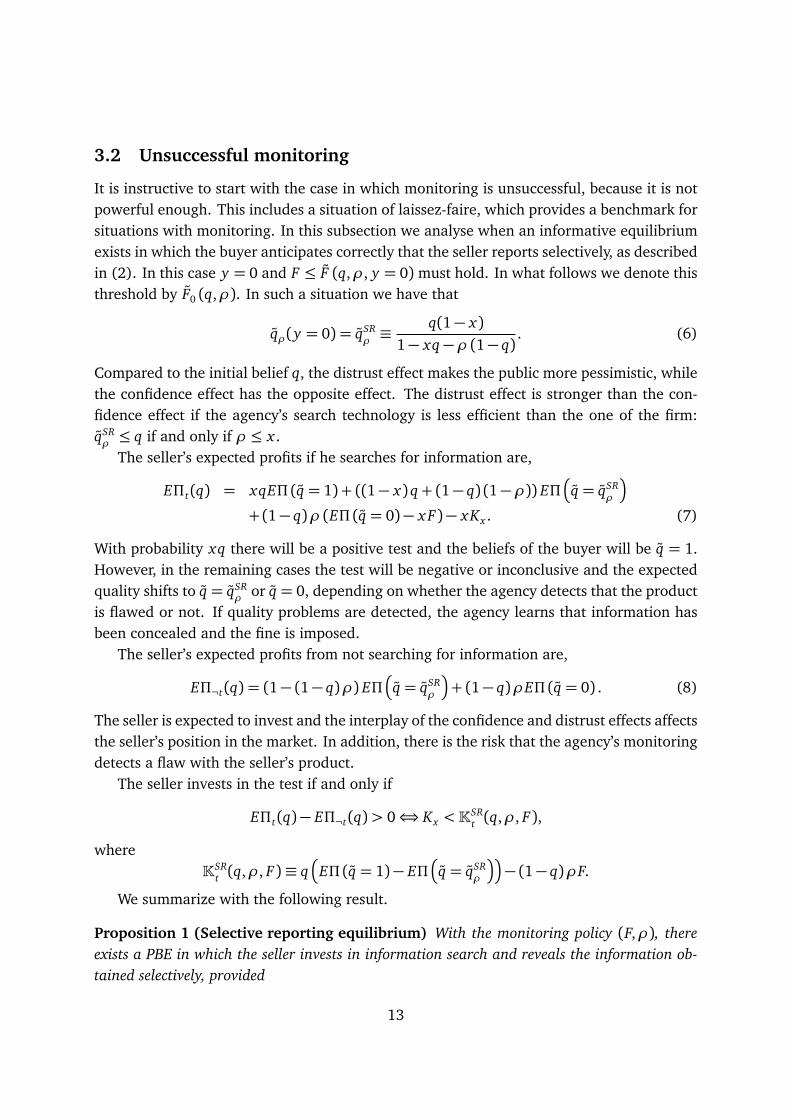
0.0 0.2 0.4 0.6 0.8 1.00.00

0.01

0.02

0.03

0.04

0.05

0.06

ρ

R

F (q, ρ, y)

Figure 1: An example for a complementary relationship

the product is detected the public’s confidence in the product increases. This confidenceeffect is reflected in EΠ

�

q = qρ�

, which increases with ρ. The overall effect is ambiguous,because the magnitude of the confidence effect depends entirely on the shape of EΠ (q).Indeed, the left hand side of (5) is closely related to the elasticity of the profit functionwith respect to q.14 Consequently, when the seller exhibits sufficient risk proclivity, themonitoring instruments can be complements. To see this consider Example 1. For this classof profit functions, the left hand side of (5) becomes λ. This is a measure of risk proclivityand Assumption 2 implies that λ > 1. As a result, whether or not for given parametervalues both monitoring policies are complements depends on the seller’s attitudes towardsrisk, which in turn is induced by the nature of the sales process in the last stage. Figure 1displays Example 1 with λ= 3 and x = q = 0.2. It illustrates a complementary relationshipfor a large interval of intermediate values of ρ; more precisely for ρ (roughly) in the interval[0.46, 0.88].

Notice that one difference between our model and Becker’s law enforcement setting isthat in Becker’s model the criminal’s payoff from committing a harmful act does not dependon a belief of the public that he is liable. This prevents the confidence effect from operating.Under these conditions EΠ

�

q = qρ�

is constant, the right hand side of (4) declines with ρ,and F and ρ are always substitutes.

14Notice that EΠ(0) = k is not required to be equal to zero and consider the increasing linear transformationf (q) = EΠ(q)− k. Replacing this expression in the left hand side of (5) yields the elasticity f ′(q)q/ f (q).

12

3.2 Unsuccessful monitoring

It is instructive to start with the case in which monitoring is unsuccessful, because it is notpowerful enough. This includes a situation of laissez-faire, which provides a benchmark forsituations with monitoring. In this subsection we analyse when an informative equilibriumexists in which the buyer anticipates correctly that the seller reports selectively, as describedin (2). In this case y = 0 and F ≤ F (q,ρ, y = 0) must hold. In what follows we denote thisthreshold by F0 (q,ρ). In such a situation we have that

qρ(y = 0) = qSRρ≡

q(1− x)1− xq−ρ (1− q)

. (6)

Compared to the initial belief q, the distrust effect makes the public more pessimistic, whilethe confidence effect has the opposite effect. The distrust effect is stronger than the con-fidence effect if the agency’s search technology is less efficient than the one of the firm:qSRρ≤ q if and only if ρ ≤ x .The seller’s expected profits if he searches for information are,

EΠt(q) = xqEΠ (q = 1) + ((1− x)q+ (1− q) (1−ρ)) EΠ�

q = qSRρ

�

+(1− q)ρ (EΠ (q = 0)− x F)− xKx . (7)

With probability xq there will be a positive test and the beliefs of the buyer will be q = 1.However, in the remaining cases the test will be negative or inconclusive and the expectedquality shifts to q = qSR

ρor q = 0, depending on whether the agency detects that the product

is flawed or not. If quality problems are detected, the agency learns that information hasbeen concealed and the fine is imposed.

The seller’s expected profits from not searching for information are,

EΠ¬t(q) = (1− (1− q)ρ) EΠ�

q = qSRρ

�

+ (1− q)ρEΠ (q = 0) . (8)

The seller is expected to invest and the interplay of the confidence and distrust effects affectsthe seller’s position in the market. In addition, there is the risk that the agency’s monitoringdetects a flaw with the seller’s product.

The seller invests in the test if and only if

EΠt(q)− EΠ¬t(q)> 0⇔ Kx <KSRt (q,ρ, F),

whereKSR

t (q,ρ, F)≡ q�

EΠ (q = 1)− EΠ�

q = qSRρ

��

− (1− q)ρF.

We summarize with the following result.

Proposition 1 (Selective reporting equilibrium) With the monitoring policy (F,ρ), thereexists a PBE in which the seller invests in information search and reveals the information ob-tained selectively, provided

13

• the monitoring technology is not powerful enough, that is, F ≤ F0 (q,ρ) and

• the test is cheap enough, that is, Kx ≤KSRt (q,ρ, F).

An example for a situation in which such an equilibrium potentially exists is laissez-faire.As ρ → 0, we have that F0 (q,ρ) →∞. Moreover, the cost threshold KSR

t is strictly posi-tive, so that the second condition holds, provided information search is cheap enough. Thebehaviour of the firm described in this informative selective reporting equilibrium mightappear cynical. But it rationalizes behaviour in line with a statement by RepresentativeHenry Waxman (D-CA) at a hearing: “The pharmaceutical industry has systematically mis-led physicians and patients by suppressing information on their drugs...,” see Couzin (2004,p. 1695).

3.3 Successful monitoring

We analyse now when an informative equilibrium exists in which monitoring induces theseller to report honestly all test results. In this case y = 1 and F ≥ F (q,ρ, y = 1)must hold.In what follows we denote this threshold by F1 (q,ρ). In such a situation we have that

qρ(y = 1) = qHRρ≡

q1−ρ (1− q)

. (9)

Notice that qHRρ> q, because on one hand, as the seller is not expected to report selectively,

the distrust effect is not present, and on the other, the confidence effect makes the publicmore optimistic than initially.

The seller’s expected profits from information search are,

EΠt(q) = xqEΠ (q = 1) + ((1− x)q+ (1− q) (1− x) (1−ρ)) EΠ�

q = qHRρ

�

+(1− q) (ρ + x (1−ρ)) EΠ (q = 0)− xKx . (10)

With probability xq there is a positive test and the beliefs of the buyer are q = 1. In theremaining cases, however, the trial is negative or inconclusive and the expected quality shiftsto q = qHR

ρor to q = 0. Profits when the seller does not invest in a test are as in (8) with qSR

ρ

replaced by qHRρ

. The seller invests in information search if and only if

EΠt(q)− EΠ¬t(q)> 0⇔ Kx <KHRt (q,ρ),

where

KHRt (q,ρ) ≡ q

�

EΠ (q = 1)− EΠ�

q = qHRρ

��

− (1− q) (1−ρ)�

E�

q = qHRρ

�

− EΠ (q = 0)�

.

The preceding yields the following result.

14

Proposition 2 (Honest reporting equilibrium) With the monitoring policy (F,ρ), there ex-ists a PBE in which the seller invests in information search and reveals honestly all informationobtained, provided

• the monitoring technology is powerful enough, that is, F ≥ F1 (q,ρ) and

• the test is cheap enough, that is, Kx ≤KHRt (q,ρ).

Lemma 1 implies that for any quality q of the firm’s product there exist monitoringpolicies (F,ρ) such that the first condition in Proposition 2 can be fulfilled. The secondcondition is similar to the one in Proposition 1 and requires that the test must be cheapenough. It remains to investigate in which circumstances this second condition may hold.

Lemma 3 The cost threshold is strictly positive, that isKHRt (q,ρ)> 0, if and only if Assumption

2 holds so that the profit function EΠ(q) has bounded average quality.

Proof: See Appendix A.2. Q.E.D.

This result is of independent interest. Related models impose convexity of the profitfunction in order to assure existence of informative equilibria with honest reporting. Lemma3 improves upon these results by uncovering a necessary and sufficient condition.15

As mentioned before, we can think of bounded average quality as imposing a (globally)convex shape on the profit function EΠ(q). The intuition is that in our model investment ininformation that is honestly reported only makes a difference if the test reveals the state ofthe world. The firm will only accept this lottery if the profit function induces risk proclivity,which is reflected in a (globally) convex shape. Indeed, Kx < KHR

t can be rearranged toyield

E�

q = qHRρ

�

< qHRρ

EΠ (q = 1) + (1− qHRρ)EΠ (q = 0)−

Kx

1−ρ(1− q).

Since the profit function induces risk proclivity, the firm prefers the gamble on the righthand side to qHR

ρwith certainty, even if it has to pay (a sufficiently low) risk premium. In

contrast, in the selective reporting equilibrium under laissez-faire (described in Proposition1 with ρ = 0) the firm is expected to invest in information and to conceal negative testresults. Rather than three there are only two outcomes, there is no gamble, and the riskattitude plays no role. As a result the cost threshold is always strictly positive.

Lastly, note that the degree of risk proclivity is also important when the profit functionEΠ(q) has bounded average quality. To see this notice that under the assumptions of Exam-ple 1 the previous condition can be rewritten as

Kx < q�

1−�

qHRρ

�λ−1�

.

15See Proposition 2 in Dahm and Porteiro (2008), Proposition 5 in Dahm et al. (2009), and Remark 1 inKamenica and Gentzkow (2011).

15

Since the right hand side of this expression is increasing in the degree of risk proclivityλ, we have that the lower λ, the lower the incentives to search for information, until inthe extreme Assumption 2 does not hold. Therefore, in this model incentives to search are‘overall continuous’ in risk attitude.

3.4 Partially successful monitoring

There is also the possibility that monitoring is only successful to some extent. This is sobecause F0 (q,ρ) < F1 (q,ρ) holds, as the minimum penalty F is increasing in the beliefand qSR

ρ< qHR

ρ. Consequently, there are some monitoring policies (F,ρ) for which a pure

strategy equilibrium at the reporting stage does not exist. For these values it is neither anequilibrium to report always honestly, nor is it an equilibrium to report always selectively.A mixed-strategy, however, allows the seller to trade-off the frequency of being caught withthe benefits from holding back negative information. More precisely, we investigate nowwhen a mixed-reporting equilibrium exists in which the selles invests in information searchand there is a certain probability that the information obtained is revealed honestly.

Consider a monitoring policy (F,ρ) with F ∈ (F0, F1) and assume that dEΠ/dq > 0holds for the relevant values for q. The seller is indifferent between reporting honestly andconcealing negative evidence if the buyer holds a belief y such that F = F (q,ρ, y). Noticethat, since F is a continuous function of y , we can apply Bolzano’s Theorem and concludethat there exists such a belief y . In what follows suppose the seller chooses y . We simplifynotation by denoting the corresponding belief of the public by qρ.

The seller’s expected profits if he searches for information are hence,

EΠt(q) = xqEΠ (q = 1)

+((1− x)q+ (1− q) (1−ρ) (x(1− y) + (1− x))) EΠ�

q = qρ�

(11)

+(1− q) ((ρ + (1−ρ)x y) (EΠ (q = 0)− xρ(1− y)F)− xKx .

This expression reduces to (7) and (10) for y = 0 and y = 1, respectively. Profits when theseller does not invest in a test are as in (8) with qSR

ρreplaced by qρ. The seller invests in the

test if and only ifEΠt(q)− EΠ¬t(q)> 0⇔ Kx <KMix

t (q,ρ, F),

where

KMixt (q,ρ, F) ≡ q

�

EΠ (q = 1)− EΠ�

q = qρ��

− (1− q) (1−ρ)y�

E�

q = qρ�

− EΠ (q = 0)�

− (1− q)ρ(1− y)F.

Since in a mixed reporting equilibrium (4) must hold with equality, the previous expressionsimplifies to

KMixt (q,ρ, F)≡ q

�

EΠ (q = 1)− EΠ�

q = qρ��

− (1− q)ρF,

16

which differs from KSRt only in the public’s belief qρ. We summarize with the following

result.

Proposition 3 (Mixed-reporting equilibrium) With the monitoring policy (F,ρ), there ex-ists a PBE in which the seller invests in information search and reveals with probability y theinformation obtained honestly, provided

• the monitoring technology is intermediately powerful, that is, F ∈ [F0, F1] and

• the test is cheap enough, that is, Kx ≤KMixt (q,ρ, F).

Notice that for F = F1 the threshold KMixt reduces to KHR

t . Similarly, for F = F0 thethreshold becomes KSR

t . This implies that, for example, for F = F0+ε with ε > 0 but small,both conditions in Proposition 3 are fulfilled, provided the test is cheap enough.

3.5 Monitoring in the absence of the firm’s information search

As usual in this type of models there might exist both an informative and a non-informativeequilibrium, depending on how expensive tests are. We now study the latter and show thatwhen the test is expensive enough there exists a PBE in which the firm is correctly expectednot to invest in tests.

If the public does not expect the firm to invest in information search, the distrust effectis not present. The beliefs of the buyer are then given by expression (9). Consequently, ifthe firm sticks to the equilibrium play and does not invest, expected profits are given by (8)with qSR

ρreplaced by qHR

ρ.

Expected profits from search depend on whether the most profitable deviation involvesselective or honest reporting. For F > F1, the most profitable deviation involves honestreporting, while selective reporting is optimal for F < F1. Consider F > F1. The seller’sexpected profits if he searches for information are given in (10). Thus, the seller invests inthe test if and only if

EΠt(q)− EΠ¬t(q)> 0⇔ Kx <K¬t(q,ρ, F) =KHRt (q,ρ).

Consider F < F1. Profits if the seller searches for information are as in (7) with qSRρ

replacedby qHR

ρ. Consequently, the seller invests in the test if and only if

EΠt(q)− EΠ¬t(q)> 0⇔ Kx <K¬t(q,ρ, F),

whereK¬t(q,ρ, F)≡ q

�

EΠ (q = 1)− EΠ�

q = qHRρ

��

− (1− q)ρF.

This implies the following result.

17

Proposition 4 (Non-informative equilibrium) With the monitoring policy (F,ρ), there ex-ists a PBE in which the seller does not invest in information search, provided the test is expensiveenough, that is,

Kx ≥K¬t(q,ρ, F)≡

¨

KHRt (q,ρ) if F ≥ F1

q�

EΠ (q = 1)− EΠ�

q = qHRρ

��

− (1− q)ρF if F ≤ F1. (12)

A non-informative equilibrium requires that the test is sufficiently expensive. Using (4)we see that the threshold K¬t(q,ρ, F) is continuous at F = F1.

3.6 The trade-off between the quality and the quantity of information

From Lemma 1 we already know that for any quality q of the firm’s product there existmonitoring policies (F,ρ) that can avoid selective reporting. An important question is howthe introduction of a monitoring policy affects the firm’s incentives for information search.In what follows we will refer to the replacement of selective reporting by honest reporting asan increase in the quality of information and to the firm’s incentives for information searchas the quantity of information. We will see that monitoring policies must balance a trade-offbetween quality and quantity of information.

We start by defining a counterpart to (12) based on Propositions 1-3 as follows

Kt(q,ρ, F)≡

KHRt (q,ρ) if F ≥ F1

KMixt (q,ρ, F) if F ∈ [F0, F1]KSR

t (q,ρ, F) if F ≤ F0

. (13)

Notice that this function is continuous at F ∈ {F0, F1}. Comparing (12) and (13), we seethat K¬t(q,ρ, F) ≤ Kt(q,ρ, F). Thus for any combination of q and Kx , there is a PBE.This equilibrium is unique if the profit function is constant on the relevant interval for q ormonitoring induces honest reporting, that is F ≥ F1. On the other hand, both an informativeand a non-informative equilibrium may exist when monitoring is unsuccessful, that is F <F1, and the profit function is strictly monotone, since qSR

ρ< qHR

ρholds.

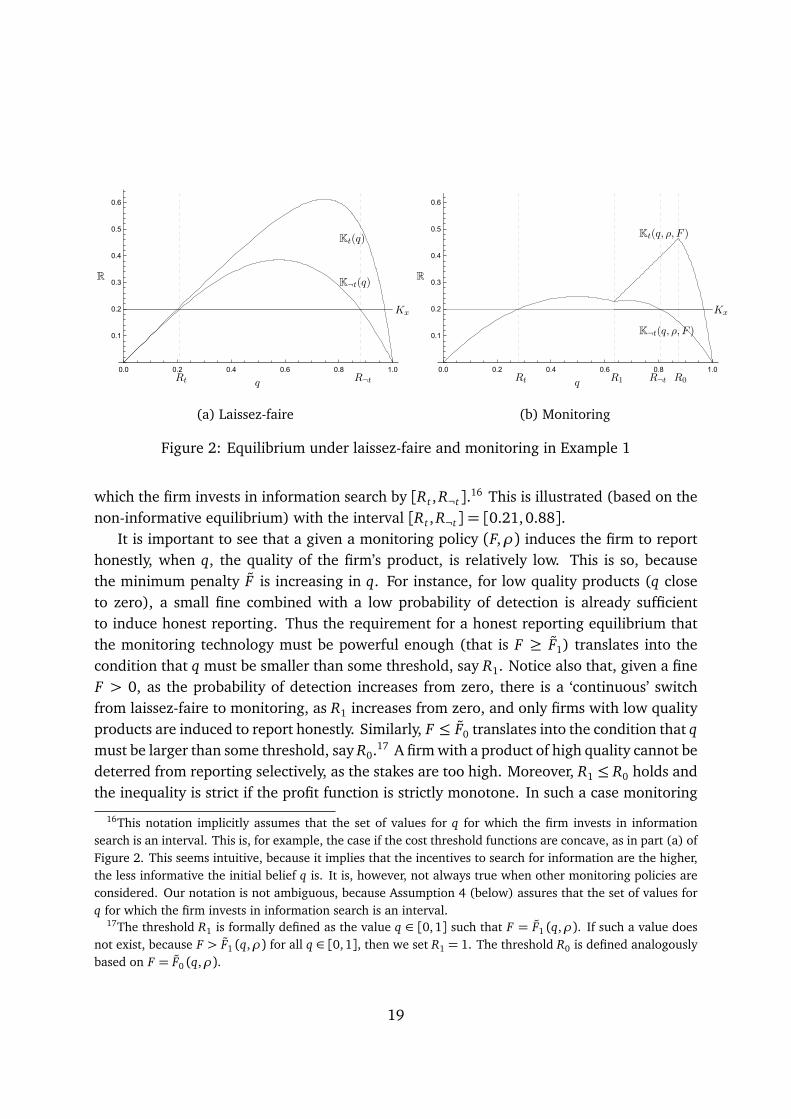
Part (a) of Figure 2 illustrates the potential multiplicity of equilibrium. The monitor-ing policy is laissez-faire. We build on Example 1, assuming in addition that λ = 2 andx = 0.75. The horizontal axis indicates q, while the vertical axis measures the cost of in-formation search Kx . For the level of cost Kx = 0.2, the firm does not invest in informationsearch if (roughly) q ∈ [0,0.2] and q ∈ [0.97, 1]; if (roughly) q ∈ [0.21, 0.88] it does investin information; and the behaviour if q ∈ [0.2, 0.21] and q ∈ [0.88, 0.97] depends on theequilibrium selection. Our results do not depend on a particular equilibrium selection, butto fix ideas we focus on the non-informative equilibrium. We denote the interval for q for

18

0.0 0.2 0.4 0.6 0.8 1.0

0.1

0.2

0.3

0.4

0.5

0.6

q

R K¬t(q)

Kt(q)

Rt R¬t

Kx

(a) Laissez-faire

0.0 0.2 0.4 0.6 0.8 1.0

0.1

0.2

0.3

0.4

0.5

0.6

ρ=0.025 and F=16

q

R

K¬t(q, ρ, F )

Kt(q, ρ, F )

Rt R1 R¬t R0

Kx

(b) Monitoring

Figure 2: Equilibrium under laissez-faire and monitoring in Example 1

which the firm invests in information search by [Rt , R¬t].16 This is illustrated (based on thenon-informative equilibrium) with the interval [Rt , R¬t] = [0.21,0.88].

It is important to see that a given a monitoring policy (F,ρ) induces the firm to reporthonestly, when q, the quality of the firm’s product, is relatively low. This is so, becausethe minimum penalty F is increasing in q. For instance, for low quality products (q closeto zero), a small fine combined with a low probability of detection is already sufficientto induce honest reporting. Thus the requirement for a honest reporting equilibrium thatthe monitoring technology must be powerful enough (that is F ≥ F1) translates into thecondition that q must be smaller than some threshold, say R1. Notice also that, given a fineF > 0, as the probability of detection increases from zero, there is a ‘continuous’ switchfrom laissez-faire to monitoring, as R1 increases from zero, and only firms with low qualityproducts are induced to report honestly. Similarly, F ≤ F0 translates into the condition that qmust be larger than some threshold, say R0.17 A firm with a product of high quality cannot bedeterred from reporting selectively, as the stakes are too high. Moreover, R1 ≤ R0 holds andthe inequality is strict if the profit function is strictly monotone. In such a case monitoring

16This notation implicitly assumes that the set of values for q for which the firm invests in informationsearch is an interval. This is, for example, the case if the cost threshold functions are concave, as in part (a) ofFigure 2. This seems intuitive, because it implies that the incentives to search for information are the higher,the less informative the initial belief q is. It is, however, not always true when other monitoring policies areconsidered. Our notation is not ambiguous, because Assumption 4 (below) assures that the set of values forq for which the firm invests in information search is an interval.

17The threshold R1 is formally defined as the value q ∈ [0,1] such that F = F1 (q,ρ). If such a value doesnot exist, because F > F1 (q,ρ) for all q ∈ [0,1], then we set R1 = 1. The threshold R0 is defined analogouslybased on F = F0 (q,ρ).

19

is sometimes successful in inducing the firm to report honestly. This likelihood y of honestreporting is the lower, the higher the initial product quality q, because ∂ qρ/∂ y > 0 impliesthat ∂ F/∂ y > 0.

Consider now the monitoring policy in part (b) of Figure 2. The monitoring policy hasF = 16 and ρ = 0.025. Again, a firm with either very low or very high product quality doesnot invest in information (and unlike in laissez-faire, the first interval does not depend onthe equilibrium selection, as F ≥ F1). Focussing again on the non-informative equilibrium,a seller in [0, Rt] and [R¬t , 1] does not invest in information, while firms in [Rt , R1] investand report honestly. All other firms invest and play a mixed reporting strategy. Since theinterval [R0, R¬t] is empty, there is no possibility of an informative equilibrium in which allinformation is reported selectively. Comparing part (b) to part (a) of Figure 2, we see thatinducing honest reporting through monitoring comes at a price, because the incentives forinformation search are reduced. More precisely, focussing on the non-informative equilib-rium, the interval [Rt , R¬t] shrinks from [0.21, 0.88] to [0.28,0.81]. But from the figureswe also see that this conclusion does not depend on the selection of equilibrium.

Our next result shows that this trade-off is general and applies to any monitoring policydifferent from laissez-faire. Such a policy increases the quality of information, becauseR1 > 0 and hence there exist values for the quality q of the firm’s product for which honestreporting is induced. Concerning the deterrence effect on the quantity of information, theproof shows the following. First, for any quality q the cost interval [0,Kt(q)] in whichsearch takes place in an informative equilibrium is larger under laissez-faire than undermonitoring. Second, the interval [K¬t(q),∞) in which search does not take place in a non-informative equilibrium is smaller under laissez-faire than under monitoring. Consequently,the incentives for information search are reduced through the introduction of monitoringand this conclusion does not depend on equilibrium selection.18

Proposition 5 Compared to laissez-faire, any monitoring policy (F,ρ) with F > 0 and ρ > 0

• increases the quality of information, that is, R1 > 0 but

• reduces the quantity of information, that is, both Kt and K¬t decrease strictly.

Proof: See Appendix A.3. Q.E.D.

This shows that optimal monitoring is determined by a trade-off. Stricter enforcementreduces the incentives for selective reporting but crowds out information search. It is worthpointing out that Assumption 2 captures the best case for monitoring. On one hand, we haveseen that if it holds, the deterrence effect is (continuously) reduced as the firm exhibits more

18This reasoning only assumes that if there is multiplicity of equilibria before and after the introduction ofmonitoring, the same type of equilibrium is played. If multiplicity of equilibria only appears before or onlyafter the introduction of monitoring, then the conclusion is unambiguous.

20

risk proclivity and the benefits from monitoring increase. On the other hand, if Assumption2 does not hold, because the profit function induces risk aversion, then the deterrence effectof monitoring is even stronger. The firm cannot be induced to report honestly, as Lemma3 does not hold. Laissez-faire outperforms all monitoring policies, whenever selectivelyreported information has a positive value for society. Therefore, in order to evaluate thedeterrence effect, it is crucial to develop a framework to assess the value of informationfor society. The next section analyses the welfare implications of monitoring in detail. Itexplores a favourable setting for monitoring, in the form of a stronger regularity conditionon profits than Assumption 2.

4 Optimal monitoring

Proposition 5 establishes the existence of a trade-off in monitoring. Investigating the optimalmonitoring policy requires to go beyond this (i) by looking at the effects of small changesin the monitoring policy and (ii) by evaluating the value of information to society. Thenext two subsections provide a framework for (i) and (ii), respectively, while the remainingsubsections investigate the optimal monitoring policy.

4.1 A sharper trade-off of monitoring under additional assumptions

In order to look at the effects of small changes in the monitoring policy we impose in thissection two additional assumptions. We first strengthen Assumptions 1 and 2 by impos-ing more structure on the shape of the profit function EΠ(q). The following condition isrelated to the notions of concave and convex functions. The difference is that concavityand convexity are based on the monotonicity of the marginal slope, while the following as-sumption requires monotonicity of the average slope. Monotonicity of the average slope isa generalization of the notion of strict star-shapedness with respect to the origin.19

Assumption 3 (Strictly increasing average quality) The profit function EΠ(q) has strictlyincreasing average quality if for each ζ ∈ (0,1) and all q we have that

ζ (EΠ(q)− EΠ(0))> EΠ(ζq)− EΠ(0). (14)19Variations of this property have appeared in the economic literature (see e.g. Landsberger and Meilijon,

1990; Chateauneuf et al., 2004; Armantier and Treich, 2009). The exact relationship between (14) belowand strict star-shapedness is as follows. Following Bullen (1998) we say that a continuous and non-negativefunction f with f (0) = 0 is strictly star-shaped (with respect to the origin) if the slope of the chord from theorigin, given by f (q)/q, is strictly increasing. This is equivalent to the requirement that for each ζ ∈ (0, 1] andall q, we have f (ζq)< ζ f (q). Notice that in our model EΠ(0) is not required to be equal to zero. If, however,EΠ(0) = 0, then (14) reduces to f (ζq)< ζ f (q).

21

The inequality in (14) is equivalent to the requirement that the slope of the chord fromEΠ(0), given by (EΠ(q)− EΠ(0))/q, must be strictly increasing. Thus Assumption 3 impliesAssumption 2. It is weaker than strict convexity of EΠ(q), because EΠ(q) can have bothconvex and concave segments. The inequality in (14) is equivalent to

dEΠ(q)dq

>EΠ(q)− EΠ(0)

q, (15)

which implies that EΠ(q) is strictly increasing. Thus Assumption 3 implies also Assumption1. Notice that Example 1 fulfils Assumption 3.

Evidence on pharmaceutical market performance seems to be consistent with Assump-tion 3. Grabowski et al. (2002) estimated a highly skewed distribution of returns (netpresent values) for new drug introductions. More precisely, the top decile of most success-ful new drugs accounted for a 52% of the total present value generated by all new drugs.This seems to suggest that market rewards higher quality at a highly increasing rate. More-over, it seems that this pattern has not changed over time. A similar analysis conducted forthe 1980–1990 period (Grabowski and Vernon, 1994) also found a highly skewed distribu-tion of returns. In this study, the top two deciles accounted for more than a 70% of the totalnet present value.

In order to introduce the second assumption, notice that the shape of the cost thresholdfunctions Kt(q,ρ, F) and K¬t(q,ρ, F) is indirectly determined through the shape of theprofit function EΠ(q). It turns out that–even imposing Assumption 3–there are situations inwhich the set of values for q for which the firm invests in information is not an interval. Infact, in the example displayed in part (b) of Figure 2 (in which Assumption 3 holds) such asituation arises for values of Kx a little higher than the cost threshold function Kt(q,ρ, F)at R1. The following assumption assures that this cannot happen. For convenience it alsorules out an interval in which the cost threshold function K¬t(q,ρ, F) is constant.

Assumption 4 (Quasiconcavity) Given a monitoring policy (ρ, F) the cost threshold func-tions Kt(q,ρ, F) and K¬t(q,ρ, F) are quasiconcave and do not have a linear portion withslope 0.

Notice that allowing for unconnected sets of values for q for which the firm invests ininformation would not provide additional insights. But it would increase the deterrenceeffects of monitoring on information search, because monitoring would reduce the quantityof information not only via Rt and R¬t but also through other thresholds. Hence, Proposition7 below might overstate the benefits of monitoring. We are now in a position to determinethe effects of small changes in the monitoring policy. The following result complementsProposition 5.

Proposition 6 Suppose a monitoring policy (ρ, F) is in place and that there is a (non-degenerate) interval of values for q for which information search takes place.An increase in the fine F

22

• reduces the quantity of information: ∂ Rt/∂ F ≥ 0 and ∂ R¬t/∂ F ≤ 0

• increases the quality of information: for y ∈ {0, 1} we have ∂ R y/∂ F > 0 and for y ∈(0,1) we have ∂ y/∂ F > 0.

An increase in the probability of detection ρ

• reduces the quantity of information:20 ∂ Rt/∂ ρ > 0 and ∂ R¬t/∂ ρ < 0

• affects the quality of information: both ∂ R y/∂ ρ > 0 for y ∈ {0, 1} and ∂ y/∂ ρ > 0 fory ∈ (0, 1) if and only if ρ and F are substitutes.

Proof: See Appendix A.4. Q.E.D.

Proposition 6 adds to Proposition 5 by formalizing the trade-off in monitoring in a differ-ent way. On one hand, the quantity of information is reduced, because the interval betweenRt and R¬t shrinks. On the other hand, however, it increases the quality of information,because it induces the firm to replace selective through honest reporting for some valuesof q. Increasing the fine has similar effects than increasing the probability of detection.There are, however, two subtle differences. First, the deterrence effect on information isstronger when stricter enforcement comes from an increase in the probability of detection,in the sense that Rt increases strictly and R¬t decreases strictly. Second, increasing the fineis more reliable in implementing stricter monitoring than increasing the probability of de-tection, unless the possibility of a complementary relationship between the instruments canbe excluded. This, however, is not the case. To see this consider again Example 1. We knowthat it fulfils Assumption 3 and in the discussion of Lemma 2 we saw that for this examplethe possibility of a complementary relationship between the probability of detection and thefine cannot be excluded. This implies that given parameter values ρ and x the firm might becharacterized by a value for q such that an increase in the probability of detection ρ mightinduce this seller to report more often selectively.

4.2 Social welfare

Analysing the welfare consequences in our setting requires defining the value of informationfor society. We postulate a social value function V (q|v) that captures the willingness to payof society for the market interaction between the firm and the public. More precisely, V (q|v)indicates the willingness to pay of society for the trading of the good when probability q is

20For simplicity of the exposition the following statement is slightly incomplete. When in case of multiplicitythe non-informative equilibrium is played or the monitoring instruments are substitutes, then the statementis correct. When, however, the non-informative equilibrium is not played and the monitoring instrumentsare complements, then ∂ Rt/∂ ρ > 0 and ∂ R¬t/∂ ρ < 0 require that the (direct) positive confidence effectof monitoring on the public’s belief is stronger than the indirect negative effect via the reduced frequency ofhonest reporting. The precise condition can be found in the proof of Proposition 6 in Appendix A.4.

23

assigned to state 1 conditional on v being the true state. For instance, V (q = 1|v = 1)measures this value when the product is of high quality and the public knows this. We donot impose any specific functional form for V (q|v) but we assume that the willingness topay is the higher, the more correct the belief is. That is, q′ ≤ q′′ implies that

V (q′′|v = 1)≥ V (q′|v = 1) and V (q′′|v = 0)≤ V (q′|v = 0). (16)

Notice that such a monotonicity imposes a minimal structure in the sense that

H(q)≡ V (q = 0|v = 0)− V (q > 0|v = 0)

measures the social harm from selective reporting and if this monotonicity is violated, thenselective reporting might be socially beneficial.21

The following expressions describe social welfare in different situations. Welfare de-pends on the monitoring policy in place, on whether the firm invests in information and,if so, how this information is reported. The following expressions are net of the cost ofinformation xKx and of the cost of monitoring ρKρ, which will both be taken into accountlater. If no investment in information takes place we have

W¬t(q,ρ)≡ qV (q = qHRρ|v = 1)+(1−q)(1−ρ)V (q = qHR

ρ|v = 0)+(1−q)ρV (0|v = 0). (17)

Since the agency always conducts tests, with probability (1− q)ρ it is revealed that the the(expected) quality of the good is low and the state of the world is v = 0. When the agency’stest is unsuccessful, the social values of information assign different values depending onthe state of the world.

On the other hand, when investment in information takes place, the three reportingstrategies must be distinguished. Successful monitoring obtains

WHRt (q,ρ)≡

xqV (q = 1|v = 1) + (1− x)qV (q = qHRρ|v = 1)

+(1− q) (1− x) (1−ρ)V (q = qHRρ|v = 0)

+(1− q)(ρ + x(1−ρ))V (q = 0|v = 0), (18)

while selective reporting yields

WSRt (q,ρ)≡

�

xqV (q = 1|v = 1) + (1− x)qV (q = qSRρ|v = 1)

+(1− q) (1−ρ)V (q = qSRρ|v = 0) + (1− q)ρV (q = 0|v = 0)

. (19)

Lastly, in the mixed-strategy equilibrium welfare is given by

WMixt (q,ρ, F) ≡ y(F,ρ)W HR

t (q,ρ) + (1− y(F,ρ))W SRt (q,ρ) (20)

= W SRt (q,ρ) + y(F,ρ)x(1− q)(1−ρ)H(qρ),

21Such a monotonicity can be derived from a micro-foundation based on a monopoly market for a medicaltreatment. Details are available upon request (and included for the convenience of the referees in AppendixB, which is not intended for publication).

24

where qρ denotes the belief of the public that makes the seller indifferent between reportinghonestly or selectively. We write y(F,ρ) in order to underline that the equilibrium frequencyof honest reporting is increasing in F and depends on ρ. Given that a test is carried out,we will also useWt(q,ρ, F) in order to indicate welfare from monitoring without specifyingwhich reporting strategy applies. More precisely,

Wt(q,ρ, F)≡

WHRt (q,ρ) if q ≤ R1(F,ρ)WMix

t (q,ρ, F) if R1(F,ρ)< q < R0(F,ρ)WSR

t (q,ρ) if q ≥ R0(F,ρ).

Notice that this function is continuous, since at R1(F,ρ) the frequency of honest reportingis one, while it is zero at R0(F,ρ).

4.3 On the optimal monitoring policy

In this subsection we analyse monitoring policies ex-ante, before the quality q of the firm’sproduct is known. At that point in time it is only known that q is distributed following thedistribution function F(q), with (continuous) probability density f (q) such that f > 0 for allq. We are now in a position to introduce the objective function of the planner. The plannerchooses a monitoring policy (ρ, F) in order to maximize

∆(F,ρ) =

∫ Rt

0

W¬t(q,ρ) f (q)dq+

∫ R¬t

Rt

[Wt(q,ρ, F)− xKx] f (q)dq (21)

+

∫ 1

R¬t

W¬t(q,ρ) f (q)dq−ρKρ.

It turns out that in general the planner’s maximization problem is not well behaved. Conse-quently, analysis of first-order conditions might not identify the optimal monitoring policy.For this reason we analyse the effects of small changes in the monitoring policy.

We focus first on the welfare effects of adjusting the fine, assuming that the probabilityof detection is positive. It turns out that increasing the fine has only two effects.

Proposition 7 The effect of a marginal increase of the fine F on social welfare can be decom-posed in two effects:

(1) The frequency of honest reporting increases, which is socially valuable:

∫ max{Rt ,min{R0,R¬t}}

max{Rt ,min{R1,R¬t}}

∂ y(F,ρ)∂ F

x(1− q)(1−ρ)H(qρ) f (q)dq ≥ 0.

25

(2) Investment in information is deterred, but the effect on welfare is ambiguous:

∂ Rt

∂ F[W¬t(Rt ,ρ)−Wt(Rt ,ρ, F) + xKx] f (Rt)

−∂ R¬t

∂ F[W¬t(R¬t ,ρ)−Wt(R¬t ,ρ, F) + xKx] f (R¬t)Ó 0.

Proof: See Appendix A.5. Q.E.D.

Increasing the fine induces more honest reporting. The model captures this through theincreased frequency with which in the mixed-reporting equilibrium information is revealedhonestly. This is formalized in part (1) of Proposition 7. Using the language of the lawenforcement literature, some social harm H(qρ) from selective reporting is avoided andthis occurs with probability x(1 − q)(1 − ρ). Thus this effect on welfare is positive. Inaddition, increasing the fine deters investment in information. This is formalized in part (2)of Proposition 7. As shown in Proposition 6, this deterrence effect on information arises,because the interval between the thresholds Rt and R¬t declines when the fine increases.The effect of deterrence on welfare is negative if and only if investment in information isdesirable at the margin.

Proposition 7 decomposes the effect of an increase of the fine on social welfare in twoeffects. It is important to note that these effects can be different from zero or not (details canbe found in the proof). For instance, when the monitoring policy is such that informationis always honestly reported whenever investment in information takes place (that is, Rt <

R¬t < R1), then both effects vanish. This is so because in equilibrium the fine is neverimposed and does not affect behaviour.

It turns out that the welfare effects of adjusting the probability of detection are morecomplex than those following an adjustment of the fine. There are two effects, which–although they are analogous to those in Proposition 9–are now both ambiguous. In addition,two new effects appear. In particular, the confidence effect induces consumers to becomemore optimistic when neither the firm nor the agency reveal the state of the world. Thisis desirable when the state of nature is good and harmful otherwise. Also, monitoring initself–as the search technology of the firm–might reveal information and reduce social harmbut has a marginal cost Kρ. Unfortunately, given the complexity of the effects and the factthat without further assumptions it is impossible to determine the overall effect, no generalconclusion can be drawn.22

The following intuition, however, suggests that Becker’s conclusion–that the probabilityof detection should be small and that the fine should be the largest possible fine–shouldalso hold in our model. If the deterrence level of a monitoring policy is higher than neededin order to induce honest reporting, then a small decrease in the probability of detection

22 Details are available upon request (and included for the convenience of the referees in Appendix B, whichis not intended for publication).

26

decreases the deterrence effect, while a decrease in the fine does not affect the incentivesto invest in information. This intuition is true if the firm can be induced to report honestlyfor all realizations of the (expected) quality q. But it leaves out the case in which this is notpossible and some selective reporting occurs for some realizations of q.

When information is (at least sometimes) selectively reported (that is, R1 < R¬t), thenthe optimal fine should not always be the largest possible fine. Key for this result is thatthe deterrence effect in part (2) of Proposition 7 is ambiguous. If selectively reported in-formation is socially undesirable, then both effects of raising the fine are aligned and socialwelfare is increased. But if selectively reported information is socially desirable, then thedeterrence effect in part (2) of Proposition 7 is negative and both effects are opposed. Insuch a case society values the information provided by the firm, although it is (at leastsometimes) selectively reported. In other words, society prefers a situation in which thefirm conducts a test and reports the result selectively to an alternative policy with a higherfine, because raising the fine deters the firm’s investment in information further. This sug-gests that the fine should be at its highest level when investment in information that is notalways reported honestly is socially undesirable. Conversely, the optimal fine might not beat its highest level when society values the firm’s information sufficiently.

In order to show that there are (reasonable) situations in which the optimal fine is notthe largest possible fine, we build in the next subsection on Brekke and Kuhn (2006) andprovide a micro-founded example of a monopoly market for a medical treatment in whichthis is the case.

4.4 Optimal monitoring in a simple example

In this subsection we consider a simple example in order to calculate explicitly social welfarefor different monitoring policies. We continue Example 1 assuming that λ = 2. The samemicro-foundations based on a monopoly market for a medical treatment that give rise tothis example imply the following functional forms for the value of information for society23

V (q|v = 1) = 2q−12

q2 and V (q|v = 0) = −12

q2. (22)

These functions capture the idea that the public decides whether or not to buy the firm’sproduct based on the information it has, which in our model is captured by q. This is an ex-ante perspective, before the state of the world is revealed. For example, if the public consistsof heterogeneous consumers and q is intermediate, then only some consumers might buythe good. If it turns out that the firm’s product is of high quality and benefits all typesof consumers, then some consumers will have been too pessimistic. Similarly, if it turnsout that the firm’s product is of low quality and harms all types of consumers, then some

23Details on this and on the calculations on which the following summary is based are available upon request(and included for the convenience of the referees in Appendix B, which is not intended for publication).

27

ρ F type of equilibrium social welfare0 any selective reporting 0.910120.025 23 honest reporting 0.973510.05 11 honest reporting 0.96736

Table 1: High efficiency of the firm’s search technology

consumers will have been too optimistic. Thus, the more correct the belief, the higher thevalues in (22).

We suppose that it is known that q = 3/4. This simplifies the calculations and helps tomake the intuitions more visible. We consider two scenarios concerning the efficiency of thefirm’s search technology. In both the quality of the firm’s test is x = 3/4 but the cost of thetest varies: Kx ∈ {0.1, 0.19}. Lastly, we assume that the cost of monitoring is Kρ = 0.3.24

Consider first the laissez-faire benchmark. Since K¬t(q) = 0.3 < Kt(q), the firm investsin the test for both efficiency levels of its search technology and there is no multiplicity ofequilibrium. Social welfare is the difference betweenWSR

t (q,ρ = 0) = 0.98512 and 0.75Kx ,which is reported in the second row of Tables 1 and 2, respectively.25

Consider monitoring and suppose first that the efficiency of the firm’s search technologyis high, that is Kx = 0.1. We start by investigating the incentives of the firm to investin a test, assuming that monitoring is successful in inducing honest reporting. From theproof of Proposition 6 it follows that KHR

t (q,ρ) is decreasing in ρ. Evaluating the extremecase KHR

t (q,ρ = 0) = 0.1875 suggests that for small detection probabilities there exists anequilibrium in which the firm invests in a test and reports the result honestly. For example,evaluating (4) we see that for a detection probability of 0.025 any fine larger than 23, orfor ρ = 0.05 any fine larger than 11, is sufficient to induce honest reporting. Indeed, forthese detection probabilities there are incentives to invest in a test, as KHR

t (q,ρ = 0.025) =0.18396 and KHR

t (q,ρ = 0.05) = 0.18038. Notice that there is no multiplicity of equilibria,as (12) and (13) coincide. Social welfare for the two policies (F,ρ) = (23,0.025) and(F,ρ) = (11, 0.05) is reported in Table 1. Notice that both policies improve over laissez-faire. Moreover, it is beneficial to decrease the detection probability as much as possible,

24A higher value for Kρ makes monitoring more costly and hence less attractive than in this example. Alower value than 0.28125 makes monitoring such an efficient search technology that the planner prefersto use it even if it has no monitoring value, because the firm does not invest in a test. This follows fromevaluating W¬t(q = 3/4,ρ) for ρ = 0 and ρ = 1, which yields 0.84375 and 1.125, respectively. Thus,0.84375> 1.125− Kρ must hold, which is equivalent to Kρ > 0.28125.

25Notice that the case in which the efficiency of the firm’s search technology is low is an example for asituation in which the firm has an incentive to conduct tests even though this is inefficient (see Jovanovic,1982; Milgrom, 2008). This is so because it is welfare improving to prohibit tests, as W¬t(q,ρ = 0) >WSR

t (q,ρ = 0)− 0.75 · 0.19.

28

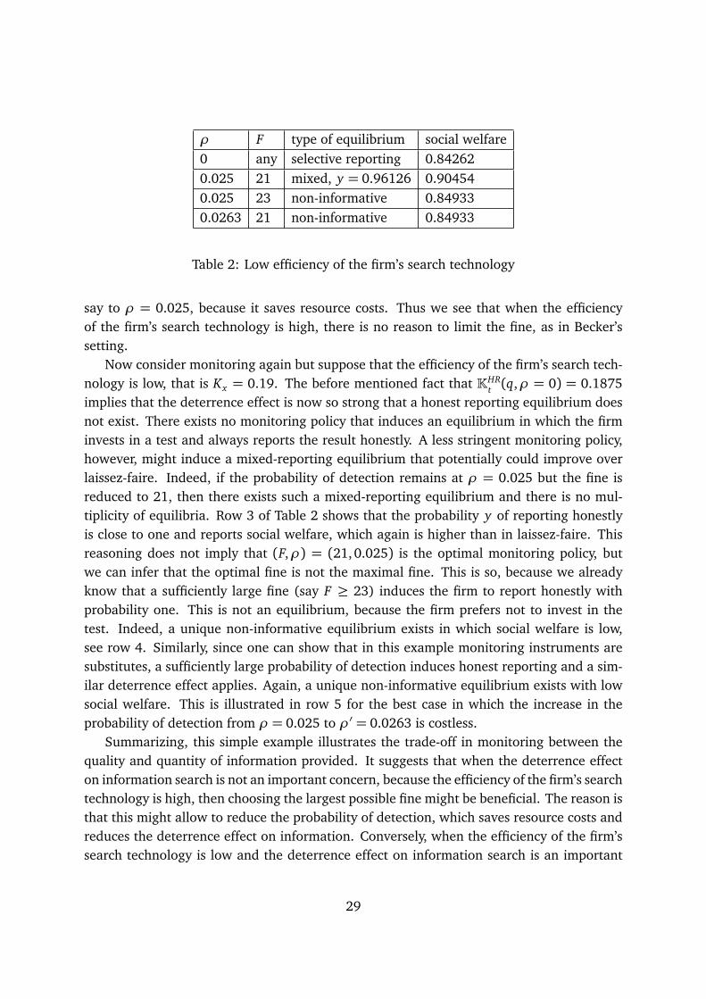
ρ F type of equilibrium social welfare0 any selective reporting 0.842620.025 21 mixed, y = 0.96126 0.904540.025 23 non-informative 0.849330.0263 21 non-informative 0.84933

Table 2: Low efficiency of the firm’s search technology

say to ρ = 0.025, because it saves resource costs. Thus we see that when the efficiencyof the firm’s search technology is high, there is no reason to limit the fine, as in Becker’ssetting.

Now consider monitoring again but suppose that the efficiency of the firm’s search tech-nology is low, that is Kx = 0.19. The before mentioned fact that KHR

t (q,ρ = 0) = 0.1875implies that the deterrence effect is now so strong that a honest reporting equilibrium doesnot exist. There exists no monitoring policy that induces an equilibrium in which the firminvests in a test and always reports the result honestly. A less stringent monitoring policy,however, might induce a mixed-reporting equilibrium that potentially could improve overlaissez-faire. Indeed, if the probability of detection remains at ρ = 0.025 but the fine isreduced to 21, then there exists such a mixed-reporting equilibrium and there is no mul-tiplicity of equilibria. Row 3 of Table 2 shows that the probability y of reporting honestlyis close to one and reports social welfare, which again is higher than in laissez-faire. Thisreasoning does not imply that (F,ρ) = (21, 0.025) is the optimal monitoring policy, butwe can infer that the optimal fine is not the maximal fine. This is so, because we alreadyknow that a sufficiently large fine (say F ≥ 23) induces the firm to report honestly withprobability one. This is not an equilibrium, because the firm prefers not to invest in thetest. Indeed, a unique non-informative equilibrium exists in which social welfare is low,see row 4. Similarly, since one can show that in this example monitoring instruments aresubstitutes, a sufficiently large probability of detection induces honest reporting and a sim-ilar deterrence effect applies. Again, a unique non-informative equilibrium exists with lowsocial welfare. This is illustrated in row 5 for the best case in which the increase in theprobability of detection from ρ = 0.025 to ρ′ = 0.0263 is costless.

Summarizing, this simple example illustrates the trade-off in monitoring between thequality and quantity of information provided. It suggests that when the deterrence effecton information search is not an important concern, because the efficiency of the firm’s searchtechnology is high, then choosing the largest possible fine might be beneficial. The reason isthat this might allow to reduce the probability of detection, which saves resource costs andreduces the deterrence effect on information. Conversely, when the efficiency of the firm’ssearch technology is low and the deterrence effect on information search is an important

29

concern, then the optimal monitoring policy might not be too stringent. This is so, becausethe deterrence effect of stricter monitoring on search for information is stronger than thepositive effect on the quality of information. Consequently, the optimal monitoring policymight not necessarily eliminate selective reporting entirely. In such a situation increasingthe probability of detection beyond the optimal monitoring policy might not be beneficial,even if doing so implies no additional costs, and the optimal fine might not be the largestpossible fine. We remark that this example does not rely on equilibrium selection, as there isno multiplicity of equilibria. In addition, since the quality of the firm’s product is known, theexample does not rely on Assumption 4. Lastly, the example is not built on a complementaryrelationship of the monitoring instruments.

5 Conclusions

The present paper contributed to deepen our understanding of the effects of enforcementof mandatory disclosure regulations. In our model a firm can invest in information aboutproduct quality and decide whether or not to disclose the findings. If the firm holds backinformation, it might be detected and fined. While we showed that such a monitoring pol-icy can improve over laissez-faire, we also saw that optimal monitoring is determined by atrade-off between the quality and quantity of information provided. Monitoring deters notonly selective reporting but also information search in the first place. This has several impli-cations. First, optimal monitoring might tolerate some selective reporting and thus it mightbe optimal to enforce mandatory disclosure rules imperfectly. Second, unlike in Becker’s(1968) law enforcement setting, the optimal fine might not be maximal. And lastly, theoptimal detection probability might be low, as in Becker’s setting–but for a different reason.Indeed, we gave an example for an optimal monitoring policy in which increasing the prob-ability of detection decreases social welfare, even when the additional resources needed arecostless. In fact our model sheds further doubt on the desirability of an increase in the prob-ability of detection. The reason is the intriguing result that the two monitoring instrumentscan be complements. Broadly speaking, if this is the case, raising the probability of detectionmight not induce more honest reporting but deter valuable investment in information.

Our persuasion game with an endogenously informed sender might also shed some lighton other situations. Consider the interaction between a firm, a rating agency and investors(see Faure-Grimaud et al., 2009). If the firm asks for a corporate governance rating and hasthe ownership of it, it might report the rating selectively. Mandatory disclosure, however,deters the firm’s incentives to pay the agency for a rating. When there is no obligation toask for a rating and ratings are valued by investors, our analysis implies that a similar trade-off between the quality and quantity of information to the one in the present paper arises.There might hence be situations in which it is optimal to enforce mandatory disclosure rulesfor ratings imperfectly.

30

Our analysis is based on a specific monitoring technology. Of course, depending on thecontext, other formulations might be reasonable. Relaxing our benchmark assumption thatthe agency only searches for evidence about quality problems would weaken the confidenceeffect. In the extreme, when the agency’s search technology is equally effective in discover-ing both states of the world, the confidence effect disappears entirely. While the possibilityof a complementary relationship between the two monitoring instruments depends on theexistence of the confidence effect, the main forces of our model do not. Even without theconfidence effect, eliminating selective reporting makes the public more optimistic. Thisincreases the opportunity costs of information search and deters investment in information.The trade-off between the quality and quantity of information formalized in Proposition 5hence is likely to be robust.

Another interesting extension of our model assumes that the firm is obliged to search forinformation. Approval of pharmaceutical products, for example, often requires the firm toconduct so-called post-marketing clinical trials but failure to comply with this requirementcreates another enforcement problem (US Food and Drug Administration, 2011; Fain etal, 2013). Monitoring policies are then two-dimensional, as the agency monitors not onlyselective reporting but also whether investment in information took place in the first place.It appears that the deterrence effect on information search is reduced, as a fine might beimposed when the firm is found out not to have searched. But analysing the overall effectsof monitoring and the optimal two-dimensional monitoring policy are challenging questionsfor future research.

Lastly, we underline that our results do not imply that stricter enforcement of disclosurerules is undesirable per se. Instead we interpret our findings as indicating the need ofquantifying the deterrence effect and the welfare consequences through empirical work.We leave these important questions for future research.

References

[1] Anderson, M. L.; K. Chiswell; E. D. Peterson; A. Tasneem; J. Topping; and R. M. Califf(2015), “Compliance with results reporting at ClinicalTrials.gov,” New England Journalof Medicine 372, p. 1031–1039.

[2] Andreoni, J. (1991), “Reasonable Doubt and the Optimal Magnitude of Fines: Shouldthe Penalty Fit the Crime?,” Rand Journal of Economics 22 (3), p. 385–395.

[3] Antman, E. M.; J. S. Bennett; A. Daugherty; C. Furberg; H. Roberts; K. A. Taubert(2007), “Use of nonsteroidal antiinflammatory drugs: an update for clinicians: ascientific statement from the American Heart Association,” Circulation 115 (12), p.1634–1642.

31

[4] Armantier, O. and N. Treich (2009), “Star-shaped probability weighting functions andoverbidding in first-price auctions,” Economics Letters 104 (2), p. 83–85.

[5] Azoulay, P. (2002), “Do pharmaceutical sales respond to scientific evidence?” Journalof Economics and Management Strategy 11 (4), p. 551–594.

[6] Becker, G.S. (1968), “Crime and punishment: an economic approach,” Journal of Po-litical Economy 76, p. 169–217.

[7] Bebchuk, L. A. and L. Kaplow (1992), “Optimal sanctions when individuals are imper-fectly informed about the probability of apprehension,” Journal of Legal Studies 21, p.365–370.

[8] Berenson, A. (2006) “A 2nd Loss For Merck Over Vioxx,” New York Times, April 6.

[9] Brekke, K.R. and M. Kuhn (2006), “Direct to consumer advertising in pharmaceuticalmarkets,” Journal of Health Economics 25, p. 102–130.

[10] Board, O. (2009), “Competition and Disclosure,” Journal of Industrial Economics 57(1), p. 197–213.

[11] Bullen, P.S. (1998), “A Dictionary of Inequalities,” Pitman Monographs and Surveys inPure and Applied Mathematics n. 97, CRC Press LLC.

[12] Chan, A.W.; F. Song; A. Vickers; et al. (2014), “Increasing value and reducing waste:addressing inaccessible research,” Lancet 383, p. 257–266.

[13] Chateauneuf, A.; M. Cohen; I. Meilijson (2004), “Four notions of mean preservingincrease in risk, risk attitudes and applications to the rank-dependent expected utilitymodel,” Journal of Mathematical Economics 40, p. 547–571.

[14] Corts K.S. (2014), “Finite Optimal Penalties for False Advertising,” Journal of Indus-trial Economics 62(4), p. 661–681.

[15] Couzin, J. (2004), “Drug research: legislators propose a registry to track clinical trialsfrom start to finish,” Science 305, p. 1695.

[16] Dahm, M.; P. González; and N. Porteiro (2009), “Trials, Tricks and Transparency: HowDisclosure Rules Affect Clinical Knowledge,” Journal of Health Economics 28, p. 1141–1153.

[17] Dahm, M. and N. Porteiro (2008), “Informational Lobbying under the Shadow of Po-litical Pressure,” Social Choice and Welfare, 30 (4), p. 531-559.

32

[18] De Angelis, C.; J.M. Drazen; F. A. Frizelle et al. (2004), “Clinical Trial Registration:A Statement from the International Committee of Medical Journal Editors,” Annals ofInternal Medicine, 141, p. 477–8.

[19] Di Tillio, A.; M. Ottaviani; and P.N. Sorensen (2015), “Persuasion Bias in Science: CanEconomics Help?,” working paper.

[20] Editorial (2013) “What a Company Knew About Its Metal Hips,” New York Times,February 10.

[21] Fain, K.; M. Daubresse; and G. Alexander (2013), “The Food and Drug AdministrationAmendments Act and Postmarketing Commitments” Journal of the American MedicalAssociation 310 (2), p. 202–204.

[22] Farell, J. (1986), “Voluntary Disclosure: Robustness of the Unraveling Result, andComments on Its Importance,” in Ronald E. Grieson, ed., Antitrust and Regulation,Lexington, MA: Lexington Books, p. 91–103.

[23] Faure-Grimaud, A.; E. Peyrache; and L. Quesada (2009), “The ownership of ratings,”Rand Journal of Economics 40 (2), p. 234–257.

[24] Feess, E. and A. Wohlschlegel (2009), “Why higher punishment may reduce deter-rence,” Economics Letters 104, p. 69–71.

[25] Fung, A.; M. Graham; D. Weil (2007), “Full Disclosure: The Perils and Promise ofTransparency,” New York, Cambridge University Press.

[26] Garoupa, N. (1997), “The theory of optimal law enforcement,” Journal of EconomicSurveys 11 (3), p. 267–295.

[27] Goldacre, B. (2013) “Health Care’s Trick Coin,” New York Times, February 1.

[28] Gopal, A. D.; N. R. Desai; T. Tse; and J. S. Ross (2015), “Reporting of NoninferiorityTrials in ClinicalTrials.gov and Corresponding Publications,” Journal of the AmericanMedical Association 313 (11), p. 1163–1165.

[29] Grabowski, H. and J. Vernon (1994), “Returns to R&D on new drug introductions inthe 1980s,” Journal of Health Economics 13, p. 383–406.

[30] Grabowski, H.; J. Vernon; and J.A. DiMasi (2002), “Returns on research and develop-ment for 1990s. New Drug Introductions,” Pharmacoeconomics 20 (3), p. 11–29.

[31] Grossman, S.J. (1981), “The Informational Role of Warranties and Private Disclosureabout Product Quality,” Journal of Law and Economics 24 (3), p. 461–483.

33

[32] Harrington, J.E. (2014), “Penalties and the Deterrence of Unlawful Collusion,” Eco-nomic Letters 124, p. 33–36.

[33] Henry, E. (2009), “Strategic disclosure of research results: The cost of proving yourhonesty,” Economic Journal 119, p. 1036–1064.

[34] Hudson, K. L. and F. S. Collins (2015), “Sharing and reporting the results of clinicaltrials,” Journal of the American Medical Association 313, p. 355–356.

[35] Jovanovic, B. (1982), “Truthful Disclosure of Information,” Bell Journal of Economics13(1), p. 36–44.

[36] Kamenica, E. and M. Gentzkow (2011), “Bayesian Persuasion,” American EconomicReview 101, p. 2590–2615.

[37] Kaplow, L. (1990), “A note on the optimal use of nonmonetary sanctions,” Journal ofPublic Economics 42, p. 245–247.

[38] Krumholz, H. M.; J. S. Ross; A. H. Presler; and D. S. Egilman (2007), “What have welearnt from Vioxx? ,” British Medical Journal 334, p.120–123.

[39] Landsberger, M. and I. Meilijson (1990), “Lotteries, insurance and star-shaped utilityfunctions,” Journal of Economic Theory 52, p. 1–17.

[40] Matthews, S. and A. Postlewaite (1985), “Quality Testing and Disclosure,” Rand Jour-nal of Economics 16 (3), p. 328–340.

[41] Milgrom, P. (1981), “Good News and Bad News: Representation Theorems and Appli-cations,” Bell Journal of Economics 12, p. 380–391.

[42] Milgrom, P. (2008), “What the seller won’t tell you: persuation and disclosure in mar-kets,” Journal of Economic Perspectives 12, p. 380–391.

[43] Milgrom, P. and J. Roberts (1986), “Relying on the Information of Interested Parties,”Rand Journal of Economics 17 (1), p. 18–32.

[44] Mookherjee, D. and I. P. L. Png (1992), “Monitoring vis-a-vis investigation in enforce-ment of law,” American Economic Review 82, p. 556–565.

[45] Polinsky, A. M. and S. Shavell (1979), “The optimal trade-off between the probabilityand magnitud of fines,” American Economic Review 69, p. 880–891.

[46] Polinsky, A. M. and S. Shavell (1991), “A note on optimal fines when wealth variesamong individuals,” American Economic Review 81, p. 618–621.

34

[47] Polinsky, A. M. and S. Shavell (2000), “The economic theory of public enforcement oflaw,” Journal of Economic Literature 38, p. 45–76.

[48] Polinsky, A. M. and S. Shavell (2010), “Mandatory Versus Voluntary Disclosure of Prod-uct Risks,” Journal of Law, Economic & Organization 28 (2), 360–379.

[49] Prayle, A. P.; M. N. Hurley; and A. R. Smyth (2012), “Compliance with mandatoryreporting of clinical trial results on ClinicalTrials.gov: cross sectional study,” The BMJ344.

[50] Seidmann, D.J. and E. Winter (1997), “Strategic information transmission with veri-fiable messages,” Econometrica 65 (1), p. 163–169.

[51] Shavell, S. (1994), “Acquisition and Disclosure of Information Prior to Sale,” RANDJournal of Economics 25 (1), p. 20–36.

[52] Shin, H. S. (1994), “The burden of proof in a game of persuasion,” Journal of EconomicTheory 64, p. 253–264.

[53] US Food and Drug Administration (2011), “Guidance for industry: postmarketingstudies and clinical trials-implementation of §505(o)(3) of the Federal Food, Drug,and Cosmetic Act,” April, available at http://www.fda.gov/downloads/Drugs/GuidanceComplianceRegulatoryInformation/Guidances/UCM172001.pdf,accessed on 20/10/2015.

[54] Wood, A.J.J. (2009) “Progress and Deficiencies in the Registration of Clinical Trials,”Special Report, New England Journal of Medicine 360, p. 824–830.

A Appendix: Proofs

A.1 Proof of Lemma 2

Consider F , the minimum value of the penalty preventing selective reporting defined in (4).Both instruments are substitutes provided ∂ F(ρ)

∂ ρ < 0, for every ρ ∈ (0, 1). Computing thederivative we obtain:

∂ F (ρ)∂ ρ

=1ρ

�

(1−ρ)dEΠdq

�

�

�

�

q=qρ

∂ qρ∂ ρ−

�

E�

q = qρ�

− EΠ (q = 0)

ρ

��

.

Using that∂ qρ∂ ρ = qρ

(1−q)1−xq−ρ(1−q) , we obtain ∂ F(ρ)

∂ ρ < 0 if and only if (5) holds. Q.E.D.

35

A.2 Proof of Lemma 3

Rewrite the cost threshold as follows

KHRt (q,ρ) = q (EΠ (q = 1)− EΠ (q = 0))

− (1−ρ (1− q))�

E�

q = qHRρ

�

− EΠ (q = 0)�

.

This implies that KHRt (q,ρ)> 0 if and only if

qHRρ(EΠ (q = 1)− EΠ (q = 0))−

�

E�

q = qHRρ

�

− EΠ (q = 0)�

> 0,

which holds if and only if (1) holds. Q.E.D.

A.3 Proof of Proposition 5

Let ρ > 0 and F > 0. We consider first the quality of information and show that R1 > 0.There are two cases.

(a) There exists q such that F = F1 (q,ρ). Notice that we have that F1 (0,ρ) = 0 if andonly if q = 0. Since F > 0, we have R1 = q > 0.

(b) There does not exist q such that F = F1 (q,ρ). Since F1 (0,ρ) = 0 and since F1 (q,ρ) =0 is weakly increasing and continuous, by the Intermediate Value Theorem we havethat F > F1 (1,ρ). By the definition of R1 we have then that R1 = 1.

We consider now the quantity of information and show that for both thresholdsK(q,ρ =0, F)−K(q,ρ > 0, F) > 0 holds. We start with Kt . Notice that Kt(q,ρ = 0, F)−Kt(q,ρ >0, F) is equal to

q�

E�

q = qHRρ

�

− EΠ�

q = qSR�

�

+φ if q ≤ R1

q�

E�

q = qρ( y)�

− EΠ�

q = qSR��

+ϕ if q ∈ (R1, R0)q�

E�

q = qSRρ

�

− EΠ�

q = qSR�

�

+ (1− q)ρF if q ≥ R0

,

where

φ ≡ (1− q) (1−ρ)�

E�

q = qHRρ

�

− EΠ (q = 0)�

> 0 and

ϕ ≡ (1− q) (1−ρ)y�

E�

q = qρ�

− EΠ (q = 0)�

+ (1− q)ρ(1− y)F > 0.

Because of the properties of qρ, we have that qHRρ≥ qρ( y) > qSR

ρ> qSR. Thus Kt(q,ρ =

0, F)−Kt(q,ρ > 0, F)> 0 for any monitoring policy (F,ρ). By analogous reasoning it can beshown that K¬t(q,ρ = 0, F)−K¬t(q,ρ, F) > 0, because K¬t(q,ρ = 0, F)−K¬t(q,ρ > 0, F)is equal to

(

q�

E�

q = qHRρ

�

− EΠ (q = q)�

+φ if q ≤ R1

q�

E�

q = qHRρ

�

− EΠ (q = q)�

+ (1− q)ρF if q ≥ R1

.

Q.E.D.

36

A.4 Proof of Proposition 6

Consider first the quality of information, that is, R1, R0 and y (F,ρ). Let

Γ ≡1−ρρ

�

E�

q = qρ�

− EΠ (q = 0)�

− F.

Notice that under Assumption 3 ∂ Γ/∂ q > 0 for any q and ∂ Γ/∂ y > 0 for any y . Hence, wehave that

∂ R y

∂ ρ= −

∂ Γ∂ ρ

∂ Γ∂ q

,∂ R y

∂ F= −

∂ Γ∂ F∂ Γ∂ q

,∂ y∂ ρ= −

∂ Γ∂ ρ

∂ Γ∂ y

, and∂ y∂ F= −

∂ Γ∂ F∂ Γ∂ y

.

Since ∂ Γ/∂ ρ < 0 if and only if the monitoring instruments are substitutes and since∂ Γ/∂ F = −1 , the statement follows.

Consider now the quantity of information, that is, Rt and R¬t . Let Rt < R1 so thatKHR

t (q,ρ) is relevant. Given Assumption 4 there are at most two values a and b such thatKHR

t (q,ρ) = xKx . Suppose that two such values a and b with a < b exist and considerγ ∈ {a, b}. We have that

∂ γ

∂ ρ= −

∂KHRt (q,ρ)∂ ρ

∂KHRt (q,ρ)∂ q

and∂ γ

∂ F= 0.

Moreover,

∂KHRt (q,ρ)

∂ ρ= (1− q)

�

E�

q = qHRρ

�

− EΠ (q = 0)�

− (1−ρ (1− q))dEΠdq

�

�

�

�

q=qHRρ

∂ qHRρ

∂ ρ< 0.

This last inequality holds, since

∂ qHRρ

∂ ρ= qHR

ρ

1− q1−ρ (1− q)

,

implies that it is equivalent to (15) holding at q = qHRρ

. Thus, under Assumption 3∂KHR

t (q,ρ)/∂ ρ < 0 for any q. On the other hand, given that a < b exist and Assump-tion 4 holds, we have that ∂KHR

t (q,ρ)/∂ q 6= 0. In fact we have that

∂KHRt (q,ρ)

∂ q

�

�

�

�

q=a

> 0 and∂KHR

t (q,ρ)

∂ q

�

�

�

�

q=b

< 0.

so that∂ a∂ ρ

> 0 and∂ b∂ ρ

< 0.

37

Now let R1 < R¬t so that

Υ (q,ρ, F)≡ q�

EΠ (q = 1)− EΠ�

q = qρ��

− (1− q)ρF

is relevant. In the previous expression qρ denotes the belief of the public in the mixed-reporting equilibrium if KMix

t = Υ applies, qρ = qSRρ

if KSRt = Υ is relevant, and qρ =

qHRρ

otherwise. Again, given Assumption 4 there are at most two values c and d such thatΥ (q,ρ, F) = xKx . Suppose that two such values c and d with c < d exist and considerγ ∈ {c, d}. We have that

∂ γ

∂ ρ= −

∂ Υ (q,ρ,F)∂ ρ

∂ Υ (q,ρ,F)∂ q

and∂ γ

∂ F= −

∂ Υ (q,ρ,F)∂ F

∂ Υ (q,ρ,F)∂ q

.

Also,

∂ Υ (q,ρ, F)∂ ρ

= −qdEΠdq

�

�

�

�

q=qρ

�

∂ qρ∂ ρ+∂ qρ∂ y

∂ y∂ ρ

�

− (1− q)F.

Notice that we can be sure that the previous expression is strictly negative, unless KMixt = Υ

applies (as only in this case ∂ y/∂ ρ 6= 0). In such a case a strictly positive sign requires themonitoring instruments to be complements and that the term in square brackets representsa sufficiently small negative number. As explained in footnote 20, we assume for simplicityof the exposition that this is not the case. Moreover,

∂ Υ (q,ρ, F)∂ F

= −qdEΠdq

�

�

�

�

q=qρ

∂ qρ∂ y

∂ y∂ F− (1− q)ρ < 0,

where again we have that ∂ y/∂ F = 0 unless KMixt = Υ applies. Again, given that c < d

exist and Assumption 4 holds, we have that ∂ Υ (q,ρ, F)/∂ q 6= 0, which similarly to the casebefore is increasing in c and decreasing in d. Thus,

∂ c∂ ρ

> 0,∂ c∂ F

> 0,∂ d∂ ρ

< 0, and∂ d∂ F

< 0.

Lastly, observe that Rt ∈ {a, c} implies that ∂ Rt/∂ ρ > 0 and ∂ Rt/∂ F ≥ 0. Similarly, R¬t ∈{b, d} implies that ∂ R¬t/∂ ρ < 0 and ∂ R¬t/∂ F ≤ 0.

A.5 Proof of Proposition 7

We start by rewriting (21). Let

a ≡min{Rt , R1} b ≡min{R1, R¬t} c ≡max{Rt ,min{R1, R¬t}} d ≡max{Rt ,min{R0, R¬t}}.

38

Remember that R1 < R0 follows, because Assumption 3 implies that the profit function isstrictly monotone. Moreover, by definition we have that Rt ≤ R¬t holds.26 The plannerchooses a monitoring policy (ρ, F) in order to maximize

∆(F,ρ) =

∫ Rt

0

W¬t(q,ρ) f (q)dq+

∫ b

a

�

WHRt (q,ρ)− xKx

�

f (q)dq (23)

+

∫ d

c

�

WMixt (q,ρ, F)− xKx

�

f (q)dq+

∫ R¬t

d

�

WSRt (q,ρ)− xKx

�

f (q)dq

+

∫ 1

R¬t

W¬t(q,ρ) f (q)dq−ρKρ

Since onlyWMixt (q,ρ, F) depends on F , the derivative of ∆(F,ρ) with respect to F is

∂

∂ F∆(F,ρ) =

∂ Rt

∂ FW¬t(Rt ,ρ) f (Rt) +

∂ b∂ F

�

WHRt (b,ρ)− xKx

�

f (b)

−∂ a∂ F

�

WHRt (a,ρ)− xKx

�

f (a) +∂ d∂ F

�

WMixt (d,ρ, F)− xKx

�

f (d)

−∂ c∂ F

�

WMixt (c,ρ, F)− xKx

�

f (c) +

∫ d

c

∂

∂ FWMix

t (q,ρ, F) f (q)dq

+∂ R¬t

∂ F

�

WSRt (R¬t ,ρ)− xKx

�

f (R¬t)−∂ d∂ F

�

WSRt (d,ρ)− xKx

�

f (d)

−∂ R¬t

∂ FW¬t(R¬t ,ρ) f (R¬t).

Consider the following six cases, which are exhaustive. Remember that Rt and R¬t onlydepend on F if they are larger than R1(F,ρ). (We disregard equalities, which would elimi-nate further terms.)

1. Let Rt < R1 < R0 < R¬t . Then (a, b, c, d) = (Rt , R1, R1, R0). Because of the continuityofWt(q,ρ, F), the second and fifth term and the fourth and eighth term cancel. Thisimplies the statement (with ∂ Rt/∂ F = 0).

2. Let R1 < Rt < R0 < R¬t . Then (a, b, c, d) = (R1, R1, Rt , R0). The second and third termand the fourth and eighth term cancel. This implies the statement.

3. Let R1 < R0 < Rt < R¬t . Then (a, b, c, d) = (R1, R1, Rt , Rt). The second and third termand the fourth and eighth term cancel. This implies the statement (with the effect inpart (1) being zero).

26To be fully precise, Rt and R¬t denote the intersections between Kx and K¬t(q,ρ, F), when the two func-tions intersect. If such an intersection does not exists, we set Rt = R¬t = 1. Assumption 4 guarantees thatthere are at most two intersections.

39

4. Let Rt < R1 < R¬t < R0. Then (a, b, c, d) = (Rt , R1, R1, R¬t). The second and fifth termand the seventh and eighth term cancel. This implies the statement (with ∂ Rt/∂ F =0).

5. Let Rt < R¬t < R1 < R0. Then (a, b, c, d) = (Rt , R¬t , R¬t , R¬t). The fourth and fifthterm and the seventh and eighth term cancel. This implies the statement (but alleffects are zero).

6. Let R1 < Rt < R¬t < R0. Then (a, b, c, d) = (R1, R1, Rt , R¬t). The second and thirdterm and the seventh and eighth term cancel. This implies the statement.

Lastly, we remark that calculating the derivative of the sixth term yields the statementin part (1) of the Proposition. Q.E.D.

40

B Appendix: Not intended for publication

This appendix is for the convenience of the referees and not intended for publication. Westart by substantiating the claims made in footnotes 10, 21 and 23 of the main text. Afterthis we provide the complete calculations for the example in Subsection 4.4. Lastly, wedecompose the welfare effects of adjusting the probability of detection, as mentioned infootnote 22.

B.1 A micro-foundation for Example 1 and Subsection 4.4

In this subsection we provide a micro-foundation for Example 1, the monotonicity propertymentioned in Subsection 4.2, and the social values postulated in expression (22) in Subsec-tion 4.4. We simplify the Hotelling model of product differentiation considered by Brekkeand Kuhn (2006) to a monopoly market for a medical treatment. We start by describing themodel and derive then Example 1 and the social values postulated in (22).

In a particular therapeutic market a continuum of patients requires medical treatment.Patients are distributed uniformly on the line segment [0,1]with mass 1. A patient’s locationl ∈ [0,1] represents disease type and/or personal characteristics. For simplicity, we considera monopolist that is located at endpoint 0 and sells a drug at a price p. The unit cost ofproduction is assumed to be zero. A patient derives the following expected utility from oneunit of the drug

U(l, p) = E(v)− sl −τp,

where E(v) > 0, s > 0, and τ ∈ [0, 1]. The parameter τ represents either the co-paymentrate or the extent to which physicians take prices into account when they make prescriptiondecisions. The term sl reflects side-effects and other factors like contraindications that re-duce the effectiveness of the drug. More precisely, there is the utility loss s that multipliesthe mismatch cost |l − 0|. Again, for simplicity we suppose that τ = s = 1. Finally, E(v)represents the expected ‘quality’ or gross effectiveness of the drug. There is also an outsidetreatment (e.g. surgery, physical exercise, or no treatment at all), the benefit of which isnormalized to zero. It is assumed that patients cannot observe their condition nor the ef-fectiveness of the two drugs. As a result, all patients consult a physician. This physician is aperfect agent for patients and has the skill to identify the condition of patients, that is, thelocation l ∈ [0, 1].

Standard calculations yield the demand function

D(p) =

1 if p ≤ E(v)− 1E(v)− p if E(v)− 1≤ p ≤ E(v)0 if E(v)≤ p

.

The monopoly price is E(v)/2 if E(v) ≤ 2 and E(v)− 1 otherwise. The profits of the mo-

41

nopolist are

EΠ (E(v)) =

0 if E(v)≤ 0(E(v))2 /4 if 0≤ E(v)≤ 2E(v)− 1 if 2≤ E(v)

.

Total (expected) surplus for society is thus

TS (E(v)) =

0 if E(v)≤ 03 (E(v))2 /8 if 0≤ E(v)≤ 2E(v)− 1/2 if 2≤ E(v)

.

Notice that this is different from ex-post total surplus for society, once the quality of thedrug is revealed.

We obtain Example 1 with λ = 2 in the following way. Consider the gross effectivenessof the drug, given by

E(v) = qu(v = 1) + (1− q)u(v = 0). (24)

One interpretation is that in state v = 0, the drug has gross effectiveness u(v = 0), while instate v = 1 effectiveness is u(v = 1). Assume u(v = 1) = 2 and u(v = 0) = 0. This implies,among other things, that for any quality q the firm has positive demand; no patient benefitsfrom the drug in the bad state but all patients benefit in the good state; and the (expected)quality is initially low enough so that a positive clinical trial can increase demand (and notjust the price). Under this assumption we have that E(v) = 2q and hence

EΠ (q) = q2 and TS (q) =32

q2.

Consider first V (q|v = 1). Since E(v) = 2q, the social value is

V (q|v = 1) =�

E(v)2

�2 12+�

2−E(v)

2

�

E(v)2= 2q−

12

q2.

Notice that this expression is increasing in q. The reason is that all consumers would ben-efit from buying the good but this does not occur because consumers are too pessimistic.Similarly,

V (q|v = 0) = −�

E(v)2

�2 12= −

12

q2,

which declines with q, as no consumer benefits from buying the good but consumers aretoo optimistic and suffer the mismatch costs. Thus, both function fulfil the monotonicityproperty mentioned in Subsection 4.2.

We obtain Example 1 for any λ > 0 by generalizing (24) to

E(v) = w(q)u(v = 1) +w(1− q)u(v = 0),

42

where w(.) is a probability weighting function (see Kahneman and Tversky (1979); Prelec(1998)). Assuming that w(.) takes the form of a power function qγ with γ > 0, whilemaintaining that u(v = 1) = 2 and u(v = 0) = 0, we obtain E(v) = 2qγ and hence EΠ (q) =q2γ. Setting γ= λ/2 yields Example 1 for any λ > 0.

Additional References

[32] Kahneman, D. and A. Tversky (1979), “Prospect Theory: An Analysis of Decision underRisk,” Econometrica 47 (2), p. 263–292.

[33] Prelec, D. (1998), “The Probability Weighting Function,” Econometrica 66 (3), p. 497–527.

B.2 Derivations of the example in Subsection 4.4

Consider the values of information for the firm. In laissez-faire we have ρ = 0 and obtain

Kt(q)≡ q�

1−�

qSRρ

�2�

and K¬t(q)≡ q�

1− q2�

.

The minimum penalty becomes

F (q,ρ, y)≡1−ρρ

�

qρ�2

,

and Kt(q,ρ, F) equals

KHRt (q,ρ) = q

�

1−�

qHRρ

�2�

− (1− q) (1−ρ)�

qHRρ

�2if q ≤ R1

KMixt (q,ρ, F) = q

�

1−�

qρ�2�

− (1− q) (1−ρ)y�

qρ�2− (1− q)ρ(1− y)F if q ∈ (R1, R0)

KSRt (q,ρ, F) = q

�

1−�

qSRρ

�2�

− (1− q)ρF if q ≥ R0

,

while

K¬t(q,ρ, F)≡

q�

1−�

qHRρ

�2�

− (1− q) (1−ρ)�

qHRρ

�2if q ≤ R1

q�

1−�

qHRρ

�2�

− (1− q)ρF if q ≥ R1

.

Consider now the values of information for society. When there is no search we obtain

W¬t(q,ρ) = qV (q|v = 1) + (1− q)(1−ρ)V (q|v = 0)

= q�

2qρ −12(qρ)

2�

− (1− q) (1−ρ)12(qρ)

2.

When monitoring deters selective reporting we obtain

WHRt (q,ρ) = xq

32+ (1− x)qqHR

ρ

�

2−12

qHRρ

�

− (1− q) (1− x) (1−ρ)12(qHRρ)2.

43

When monitoring is unsuccessful welfare is given by

WSRt (q,ρ) = xq

32+ (1− x)qqSR

ρ

�

2−12

qSRρ

�

− (1− q) (1−ρ)12(qSRρ)2.

Lastly, the mixed-strategy equilibrium yields

WMixt (q,ρ, F) =W SR

t (q,ρ) + y(F,ρ)x(1− q)(1−ρ)12(qρ)

2.

B.3 The welfare effects of adjusting the probability of detection

We decompose now the effects of adjusting the probability of detection, assuming that thefine is positive. For notational simplicity we provide a result for the case in which all threetypes of informative equilibria (honest, selective and mixed-reporting) can occur, dependingon the realised quality q of the firm’s product. More precisely, suppose that Rt < R1 <

R0 < R¬t . This case seems particularly relevant, because the monitoring policy has somesuccess in eradicating selective reporting but it falls short from eliminating it completely. Itis straightforward to adjust the argument to the other cases.

It turns out that increasing the probability of detection has complex effects. Some ofthe consequences are similar to the effects of raising the fine described in Proposition 7 butfurther effects emerge. In order to offer a compact representation of the different effects,the following statement uses the notation x ∈ {0, x} and y ∈ {0, y}, where x and y areequal to x and y , respectively, if (for a given value of q) the firm invests in information andzero otherwise. Remember also that y—the probability that the firm reports honestly—isequal to zero in a selective reporting equilibrium.

Proposition 8 The effect of a marginal increase of the probability of detection ρ on socialwelfare can be decomposed in four effects, each of which is ambiguous:

(1) The frequency of honest reporting changes:

∫ R0

R1

∂ y(F,ρ)∂ ρ

x(1− q)(1−ρ)H(qρ) f (q)dq.

(2) Investment in information is deterred:

∂ Rt

∂ ρ

�

W¬t(Rt ,ρ)−WHRt (Rt ,ρ) + xKx

�

f (Rt)

−∂ R¬t

∂ ρ

�

W¬t(R¬t ,ρ)−WSRt (R¬t ,ρ) + xKx

�

f (R¬t).

44

(3) The confidence effect induces the public to be more optimistic:

∫ 1

0

∂ qρ∂ ρ

�

(1− x)q∂ V (q = qρ|v = 1)

∂ q

�

�

�

�

q=qρ

+ (1− x y(F,ρ))(1− q)(1−ρ)∂ V (q = qρ|v = 0)

∂ q

�

�

�

�

q=qρ

�

f (q)dq

(4) Monitoring in itself reveals information and reduces social harm but causes a resourcecost:

∫ 1

0

(1− q)(1− x y(F,ρ))H(qρ) f (q)dq− Kρ.

We next compare this result to Proposition 7 and offer then a proof. The first two effectsare analogous to the corresponding ones in Proposition 7. There are, however, two addi-tional twists that mirror the discussion after Proposition 6. On the one hand, the frequencyof honest reporting might decline, so that the first effect might be negative. On the otherhand, the deterrence effect on information is stronger in the sense that the second termis unambiguously negative (and never zero).27 An increase in the probability of detectionalways crowds out honestly reported information.

There are two additional effects that are not present in Proposition 7. A third effectarises, because the confidence effect induces consumers to become more optimistic whenneither the firm nor the agency reveal the state of the world. This is desirable when thestate of nature is good and harmful otherwise. The latter negative effect applies less often,the higher the frequency of honest reporting (that reveals the state of the world). Lastly,monitoring—as the search technology of the firm—has a marginal resource cost Kρ andmight reveal the state of the world when the firm does not reveal it. Again, this happensless often, the higher the frequency of honest reporting.

27The conclusion that the deterrence effect is negative assumes that honestly reported information is so-cially desirable at the margin, so that the incentives for strict monitoring are highest. If honestly reportedinformation is not desirable, then the deterrence effect is positive (but never zero).

45

Proof: The derivative of ∆(F,ρ) with respect to ρ is

∂

∂ ρ∆(F,ρ) =

∂ Rt

∂ ρW¬t(Rt ,ρ) f (Rt) +

∫ Rt

0

∂

∂ ρW¬t(q,ρ) f (q)dq

+∂ R1

∂ ρ

�

WHRt (R1,ρ)− xKx

�

f (R1)−∂ Rt

∂ ρ

�

WHRt (Rt ,ρ)− xKx

�

f (Rt)

+

∫ R1

Rt

∂

∂ ρWHR

t (q,ρ) f (q)dq+∂ R0

∂ ρ

�

WMixt (R0,ρ, F)− xKx

�

f (R0)

−∂ R1

∂ ρ

�

WMixt (R1,ρ, F)− xKx

�

f (R1) +

∫ R0

R1

∂

∂ ρWMix

t (q,ρ, F) f (q)dq

+∂ R¬t

∂ ρ

�

WSRt (R¬t ,ρ)− xKx

�

f (R¬t)−∂ R0

∂ ρ

�

WSRt (R0,ρ)− xKx

�

f (R0)

+

∫ R¬t

R0

∂

∂ ρWSR

t (q,ρ) f (q)dq+∂ R¬t

∂ ρW¬t(R¬t ,ρ) f (R¬t)

+

∫ 1

R¬t

∂

∂ ρW¬t(q,ρ) f (q)dq− Kρ.

Because of the continuity ofW(q,ρ, F), the third and seventh term cancel; and similarlyfor the sixth and tenth term. Rearranging we are left with

∂

∂ ρ∆(F,ρ) =

∂ Rt

∂ ρW¬t(Rt ,ρ) f (Rt) +

∫ Rt

0

∂

∂ ρW¬t(q,ρ) f (q)dq

+∂ R¬t

∂ ρ

�

WSRt (R¬t ,ρ)− xKx

�

f (R¬t)−∂ Rt

∂ ρ

�

WHRt (Rt ,ρ)− xKx

�

f (Rt)

+

∫ R1

Rt

∂

∂ ρWHR

t (q,ρ) f (q)dq+

∫ R0

R1

∂

∂ ρWMix

t (q,ρ, F) f (q)dq

+

∫ R¬t

R0

∂

∂ ρWSR

t (q,ρ) f (q)dq+∂ R¬t

∂ ρW¬t(R¬t ,ρ) f (R¬t)

+

∫ 1

R¬t

∂

∂ ρW¬t(q,ρ) f (q)dq− Kρ.

The first, third, fourth and eighth term of the previous expression prove part (2) of the

46

proposition. Consider the second and penultimate term. We have that

∂

∂ ρW¬t(q,ρ) = q

∂ V (q = qHRρ|v = 1)

∂ q

�

�

�

�

�

q=qHRρ

∂ qHRρ

∂ ρ

+(1− q)(1−ρ)∂ V (q = qHR

ρ|v = 0)

∂ q

�

�

�

�

�

q=qHRρ

∂ qHRρ

∂ ρ

+(1− q)H(qHRρ).

Consider the fifth term. We have that

∂

∂ ρWHR

t (q,ρ) = (1− x)q∂ V (q = qHR

ρ|v = 1)

∂ q

�

�

�

�

�

q=qHRρ

∂ qHRρ

∂ ρ

+(1− x)(1− q)(1−ρ)∂ V (q = qHR

ρ|v = 0)

∂ q

�

�

�

�

�

q=qHRρ

∂ qHRρ

∂ ρ

+(1− x)(1− q)H(qHRρ).

Consider the seventh term. This yields

∂

∂ ρWSR

t (q,ρ) = (1− x)q∂ V (q = qSR

ρ|v = 1)

∂ q

�

�

�

�

�

q=qSRρ

∂ qSRρ

∂ ρ

+(1− q)(1−ρ)∂ V (q = qSR

ρ|v = 0)

∂ q

�

�

�

�

�

q=qSRρ

∂ qSRρ

∂ ρ

+(1− q)H(qSRρ).

Consider the sixth term. We obtain

∂

∂ ρWMix

t (q,ρ, F) =∂

∂ ρWSR

t (q,ρ) +∂ y(F,ρ)∂ ρ

x(1− q)(1−ρ)H(qρ)

−x(1− q)(1−ρ)y(F,ρ)∂ V (q = qρ|v = 0)

∂ q

�

�

�

�

q=qρ

∂ qρ∂ ρ

−x(1− q)y(F,ρ)H(qρ).

Notice that the second term on the right hand side of this last expression proves part (1) ofthe proposition, while collecting and rearranging the remaining terms using the notation xand y completes the proof of parts (3) and (4). Q.E.D.

47