the electrical environment of the earth's atmosphere: a … · the electrical environment of...

THE ELECTRICAL ENVIRONMENT OF THE EARTH’SATMOSPHERE: A REVIEW

D.K. SINGH1, R.P. SINGH2 and A.K. KAMRA1

1Indian Institute of Tropical Meteorology, Pune-411 008, [email protected], [email protected]

2Department of Physics, Banaras Hindu University, Varanasi-211 005, India

Abstract. The study of the electrical environment of the Earth’s atmosphere has rapidly advancedduring the past century. Great strides have been made towards the understanding of lightning andthunderstorms and in relating them to the global electric circuit. The electromagnetic fields andcurrents connect different parts of the Earth’s environment, and any type of perturbation in one regionaffects another region. Starting from the traditional views in which the electrodynamics of one regionhas been studied in isolation from the neighboring regions, the modern theory of the global electricalcircuit has been discussed briefly. Interconnection and electrodynamic coupling of various regions ofthe Earth’s environment can be easily studied by using the global electric circuit model. Deficienciesin the model and the possibility of improvement in it have been suggested. Application of the globalelectric circuit model to the understanding of the Earth’s changes of climate has been indicated.

1. Introduction

The Earth’s environment is filled with electrons, negative ions and positive ions,comprising of very low plasma density. These charged particles interact amongstthemselves and also interact with electric and magnetic fields present in the me-dium, leading to the control of space–plasma environments by an electrodynamicprocess. The outer boundary of the Earth’s environment extends up to the mag-netosphere, which is formed by interaction of the solar wind with the geomagneticfield (Hines, 1963; Dungey, 1978). As a result of this interaction the geomagneticfield is compressed on the dayside, and a tail trailing up to a distance of more than500 Earth radii is created on the nightside (Dungey, 1978). The electric currentdeveloped in the magnetopause helps in the creation of the tail. The cavity carvedas a result of the deflection of the solar wind by the geomagnetic field and enclosedby the magnetopause is called magnetosphere (Figure 1), in which the geomagneticfield is contained. The magnetosphere contains the radiation belt composed ofenergetic charged particles trapped in the magnetic field. The number density ofelectron - ion pairs in the magnetosphere is highly variable, ranging in order ofmagnitude from a low of 106 m−3 in parts of the tail up to 1012 m−3 in the densestportions of the dayside atmosphere. As a result of the solar wind’s interaction withthe geomagnetic field, mass, momentum, and energy are transferred from the solarwind to the magnetosphere, and a complex pattern of several current systems is

Space Science Reviews 113: 375–408, 2004.© 2004 Kluwer Academic Publishers. Printed in the Netherlands.

376 SINGH ET AL.

Figure 1. Three-dimensional schematic diagram of the Earth’s magnetosphere (thin arrows indicatethe direction of the magnetic field and thick arrows show the magnetopause’s current, ring current,field-aligned current, neutral sheet current, and tail current).

generated in different parts of the magnetosphere (Figure 1). The variability of solarconditions reflects in the variability of the solar wind, which results in variability ofthe current system. In the magnetosphere a natural phenomenon involving electricdischarge, somewhat like a thunderstorm, occurs which is called a magnetosphericsubstorm. During substorms the cross-tail current is disrupted and diverted towardsthe ionosphere as a field-aligned current. The energy stored in the magnetotail isconverted into plasma heat and bulk flow energy, and it is dumped towards the innermagnetosphere. Energetic precipitating particles cause enhanced auroral activity.

Relations between atmospheric electricity and both solar activity (Cobb, 1967;Markson, 1971, 1978; Hays and Roble, 1979; Roble and Hays, 1979; Markson andMuir, 1980; Roble and Tzur, 1986; Roble, 1991; Tinsley and Heelis, 1993; Rycroftet al., 2000; Tinsley, 2000) and volcanic activity (Meyerott et al., 1983) have beenreported. Any perturbation in the interplanetary or atmospheric environment causesa variation in electrical conductivity and hence variation in the current/electricfield system of the atmosphere. The atmospheric electric conductivity depends onthe ionization rate, the recombination rate, and various meteorological and solaractivity conditions. In the ionosphere ionization is caused mainly by the extremeultraviolet and X-ray radiation from the Sun. The precipitating energetic chargedparticles from the magnetosphere can cause significant ionization, mainly at highlatitudes. The ionization in the lower atmosphere depends on solar activity in thesense that at a particular height the ion production rate is lower during the sunspotmaximum period than during the sunspot minimum period (Neher, 1967). Themechanism is not fully understood, but it appears that irregularities and enhance-ments of the interplanetary magnetic field (IMF) tend to exclude part of the lower

THE ELECTRICAL ENVIRONMENT OF THE EARTH’S ATMOSPHERE 377

energy cosmic rays from the inner solar system (Barouch and Burlaga, 1975). Theeffect becomes more pronounced with increasing height/increasing geomagneticlatitude (L). At L = 50◦ the reduction of the ion production rate during the periodsof sunspot maximum is about 30% at 20 km and about 50% at 30 km (Gringelet al., 1986). The solar cycle dependence was confirmed by measurement with theopen balloon-borne ionization chambers (Hofmann and Rosen, 1979). Analyticalexpressions for computing the ionization rates dependent on latitude and the periodof solar cycles are given by Heaps (1978). Superimposed on the 11 year solar cyclevariation are the Forbush decreases, which are somehow related to solar flares andexhibit a temperature reduction of the incoming cosmic ray flux for periods of afew hours to a few days or weeks (Duggal and Pomerantz, 1977).

Measurements of electric current and fields in the lower atmosphere show vari-ations associated with solar flares (Cobb, 1967; Muhleisen, 1971; Holzworth andMozer, 1979; Michnowski, 1998; Tinsley, 2000), solar magnetic sector boundarycrossings (Markson, 1971, Park, 1976), geomagnetic activity (Cobb, 1967; Marcz,1976; Tanaka et al., 1977; Bering et al., 1980), auroral activity (Freier, 1961; Olson,1971; Lobodin and Paramonov, 1972; Shaw and Hunsucker, 1977), and solar cyclevariations (Muhleisen, 1977; Olson, 1977; Tinsley, 2000). A specific mechanismfor the solar terrestrial coupling through atmospheric electricity has been sugges-ted and studied (Markson, 1971, 1978; Markson and Muir, 1980; Roble, 1985;Lakhina, 1993; Rycroft et al., 2000). In this paper we present briefly the electricalstructure of the Earth’s atmosphere, source of electric field, and its connectionwith the global electric circuit (GEC). Recent results in this emerging field aresummarized.

2. Electrical Structure of the Earth’s Atmosphere

It has been known for over two centuries that the solid and liquid Earth and itsatmosphere are almost permanently electrified. The surface has a net negativecharge, and there is an equal and opposite positive charge distributed throughout theatmosphere above the surface. The Earth’s atmosphere has been studied by divid-ing it into various regions based on temperature profiles, conductivity, or electrondensity (Figure 2). Each region has been studied more or less in isolation as faras electrodynamical processes are concerned, although processes operating in oneregion are influenced by the presence of neighboring regions and the processes atwork in them.

2.1. THE TROPOSPHERE

The lowest region of the atmosphere, where the temperature decreases with anincrease in altitude, is called the troposphere, and which is the chief focus ofmeteorologists, for it is in this layer that essentially all phenomena to which we

378 SINGH ET AL.

Figure 2. Profiles distribution of the temperature, conductivity, and electron density of the Earth’satmosphere.

collectively refer as weather occur. Almost all clouds, and certainly all precipita-tion, as well as all the violent storms, occur in this region of the atmosphere. Thereshould be little wonder why the troposphere is often called as the ‘weather sphere’.It extends from the surface of the Earth up to about 10 to 12 km. Throughout thislayer there is a general decrease of temperature with altitude at a mean rate of6.5 ◦C/km, which is called the environmental lapse rate. This lapse rate is highlyvariable from place to place, but never exceeds 10 ◦C/km, except near the ground.Sometimes shallow layers up to about 1 km deep in which the temperature actuallyincreases with height are observed in the troposphere. When such a reversal occursa temperature inversion is said to exist.

The main source of ionization in the troposphere is galactic cosmic rays, apartfrom radioactive materials exhaling from the soil. The radioactive ionization com-ponent depends on different meteorological parameters and can exceed the cosmicrays component by an order of magnitude (Hoppel et al., 1986). It decreases rap-idly with increasing height, and at 1 km it is already significantly less than thecontribution owed to cosmic rays (Pierce and Whitson, 1965).

The temperature of the Earth’s surface rises as a result of absorption of solarradiation. Heat from the Earth’s surface is transferred to the air near the groundby conduction and radiation, and is distributed upwards through the atmosphere byturbulent mixing. Convection, which involves the ascent of warm air and downwardmovement of cold air is effective in transporting heat upward. Owing to this process


the average air temperature is usually highest near the ground and decreases withheight until it reaches a level called the tropopause, at an average height of approx-imately 12 km in the tropics and 10 km near the poles. The minimum temperatureat the tropopause level can be between −70 ◦C to −90 ◦C in the tropics.

2.2. THE STRATOSPHERE

The stratosphere lies between the tropopause and the stratopause (∼ 50 km alti-tude). In the lower part of the stratosphere the temperature is nearly constant withheight or increases slowly. Throughout the stratosphere galactic cosmic rays providethe principal ionization source, and the ionization rate does not vary diurnally butdoes vary with geomagnetic latitude and with the phase of the 11 year solar cycle.Roughly speaking, the ion production rate at 30 km height increases by a factorof 10 from the geomagnetic equator to the polar caps at a sun spot minimum(cosmic-ray maximum) and by a factor of 5 at a sun spot maximum. The solarcycle modulation is near zero at the equator, increasing to a factor of about 2 in apolar cap region. The ionization rate above 30 km is approximately proportionalto the atmospheric density. These properties result because of (a) the shieldingeffect of the geomagnetic field, which allows cosmic ray particles to enter theatmosphere at successively higher latitudes for successively lower energies, and(b) the reduction in cosmic ray flux in the inner solar system as solar activityintensifies. In addition, solar proton events (SPE) provide a sporadic and intensesource of ionization at high latitudes. Solar flares produced one of the largest SPEevent recorded in terms of the total energy input into the middle atmosphere during4–9 August, 1972. The largest Forbush decrease in cosmic rays intensity that hasbeen observed also occurred during this event (Pomerantz and Duggal, 1973, 1974;Duggal, 1979). The conductivity, which is roughly of the order of 10−14 mho/mat the Earth’s surface, increases exponentially with altitude in the troposphere -stratosphere region; the main charge carriers are the small positive and negativeions. The warming of the stratosphere results from the absorption of ultravioletradiation by ozone (at wavelengths between about 200 nm and 310 nm). Althoughthe stratosphere contains much of the total atmospheric ozone (peak density ∼ 20–22 km), the maximum temperature occurs at the stratopause, where the temperaturemay exceed 0 ◦C.

2.3. THE MESOSPHERE

This is the region of the second decrease of temperature with height, like the tro-posphere, to a minimum of about −90 ◦C around 80 km. This layer is commonlyknown as the mesosphere, which literally means the middle sphere and the levelcorresponding to the minimum temperature is referred to as the mesopause. Themesosphere extends from about 50 km to 85 km, and many of the atmosphericvariations encountered in it are linked to complicated processes in the underlyinglayers. The major sources of ionization are the solar Lyman alpha radiation, X-ray

380 SINGH ET AL.

radiation, and the intense auroral particle precipitation. The conductivity increaseswith height rather sharply. The main charge carriers are electrons, positive ions(e.g., N+

2 O+2 , NO+) and the negative ions O−

2 . The major daytime source of ion-ization in undisturbed conditions is provided by the NO molecule, whose lowionization potential of 9.25 electron volts allows it to be ionized by the intenseSolar Lyman alpha radiation. The concentration of NO in the mesosphere is notwell known and is almost certainly variable in response to meteorological factors(Solomon et al., 1982).

2.4. THE IONOSPHERE

The ionosphere starts from above the mesopause and extends to a height of about500 km. The upper boundary is not well defined, i.e., the so called thermosphereis included in the ionosphere. In this region ionized species do not necessarilyrecombine quickly, and there is a permanent population of ions and free electrons.The net concentration of ions and free electrons (generally in equal numbers) isgreatest at a height of a few hundred kilometers and has a profound effect onthe properties and behavior of the medium. The major sources of ionization areEUV and X-rays radiation from the sun, and energetic particle precipitation fromthe magnetosphere into the auroral ionosphere. The Current carriers are electronsand the positive ions such as NO+, O+

2 , and O+. Electrical conductivity becomesanisotropic in this region with the parallel conductivity (with respect to an Earth’sfield line) exceeding the transverse conductivity by several orders of magnitude.The ionized medium also affects radio waves, and as a plasma it can support andgenerate a variety of waves, interactions, and instabilities which are not found in aneutral gas.

2.5. THE MAGNETOSPHERE

The magnetic field decreases with altitude as the atmosphere becomes more sparseand its degree of ionization increases. The electrodynamic properties of the me-dium above the ionosphere are dominated by the geomagnetic field, and this regionis called the magnetosphere. The lower boundary of the magnetosphere is theionosphere and it extends up to magnetopause. At the magnetopause energy iscoupled into the magnetosphere from the solar wind, and here is determined muchof the behavior of the magnetosphere and of the ionosphere at high latitudes. Inthe sunward direction the magnetopause is encountered at about 10 Earth radii, butin the anti-solar direction the magnetosphere is extended downward in a long tail,the magnetotail, within which occur plasma processes of great significance for thegeospacial regions.


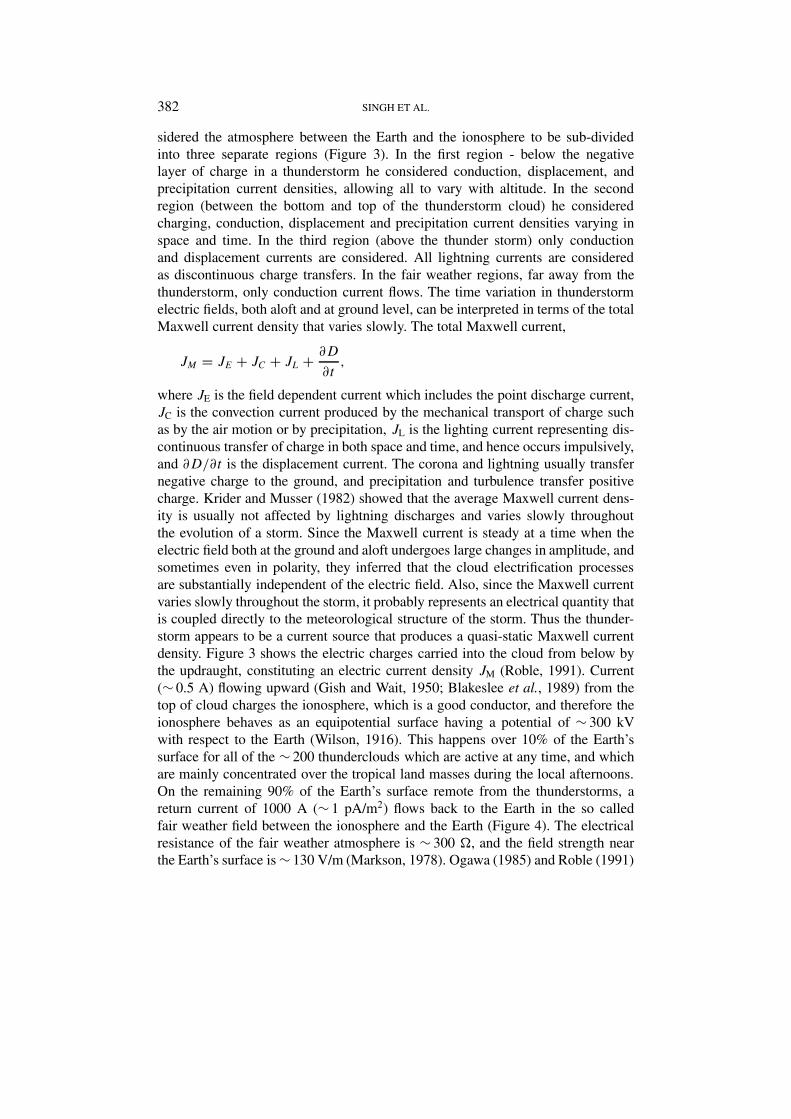
Figure 3. Various currents which flow in the vicinity of an active thunder cloud. There are fivecontributions to the total current (the Maxwell current) JM = JE +JC +JL +JP +∂D/∂t , below thethunder clouds. Above the thunder cloud, JM = JE + ∂D/∂t . Here, JE = σE is the field-dependentcurrent, JC is the convection current, JL is the lightning current, JP is the precipitation current, and∂D/∂t is the displacement current (Roble, 1991).

3. Sources of electric fields in different regions and their coupling

A thunderstorm is the main source of electric fields in the lower atmosphere com-prised of the troposphere, stratosphere, and mesosphere. The thunderstorm activityproduces vertical electric fields on a global scale. The main negative charge in thelower part of a thunderstorm occurs at a height at which the atmospheric temper-ature is between −10 ◦C and −20 ◦C (this temperature range is typically between6 to 8 km for summer and 2 km for winter thunderstorms) (Krehbiel et al., 1979).The positive charge at the top of the storm does not have so clear a relationshipwith temperature as the negative charge, but can typically occur between −25 ◦Cand −60 ◦C depending on the size of the storm (this temperature range usually liesbetween 8 to 16 km in altitude).

There is no generally accepted model of thunderstorm electrification that canbe used to calculate the current which storms release into the GEC. Freier (1979)presented a thunderstorm model with more details than the other models. He con-

382 SINGH ET AL.

sidered the atmosphere between the Earth and the ionosphere to be sub-dividedinto three separate regions (Figure 3). In the first region - below the negativelayer of charge in a thunderstorm he considered conduction, displacement, andprecipitation current densities, allowing all to vary with altitude. In the secondregion (between the bottom and top of the thunderstorm cloud) he consideredcharging, conduction, displacement and precipitation current densities varying inspace and time. In the third region (above the thunder storm) only conductionand displacement currents are considered. All lightning currents are consideredas discontinuous charge transfers. In the fair weather regions, far away from thethunderstorm, only conduction current flows. The time variation in thunderstormelectric fields, both aloft and at ground level, can be interpreted in terms of the totalMaxwell current density that varies slowly. The total Maxwell current,

JM = JE + JC + JL + ∂D

∂t,

where JE is the field dependent current which includes the point discharge current,JC is the convection current produced by the mechanical transport of charge suchas by the air motion or by precipitation, JL is the lighting current representing dis-continuous transfer of charge in both space and time, and hence occurs impulsively,and ∂D/∂t is the displacement current. The corona and lightning usually transfernegative charge to the ground, and precipitation and turbulence transfer positivecharge. Krider and Musser (1982) showed that the average Maxwell current dens-ity is usually not affected by lightning discharges and varies slowly throughoutthe evolution of a storm. Since the Maxwell current is steady at a time when theelectric field both at the ground and aloft undergoes large changes in amplitude, andsometimes even in polarity, they inferred that the cloud electrification processesare substantially independent of the electric field. Also, since the Maxwell currentvaries slowly throughout the storm, it probably represents an electrical quantity thatis coupled directly to the meteorological structure of the storm. Thus the thunder-storm appears to be a current source that produces a quasi-static Maxwell currentdensity. Figure 3 shows the electric charges carried into the cloud from below bythe updraught, constituting an electric current density JM (Roble, 1991). Current(∼ 0.5 A) flowing upward (Gish and Wait, 1950; Blakeslee et al., 1989) from thetop of cloud charges the ionosphere, which is a good conductor, and therefore theionosphere behaves as an equipotential surface having a potential of ∼ 300 kVwith respect to the Earth (Wilson, 1916). This happens over 10% of the Earth’ssurface for all of the ∼ 200 thunderclouds which are active at any time, and whichare mainly concentrated over the tropical land masses during the local afternoons.On the remaining 90% of the Earth’s surface remote from the thunderstorms, areturn current of 1000 A (∼ 1 pA/m2) flows back to the Earth in the so calledfair weather field between the ionosphere and the Earth (Figure 4). The electricalresistance of the fair weather atmosphere is ∼ 300 �, and the field strength nearthe Earth’s surface is ∼ 130 V/m (Markson, 1978). Ogawa (1985) and Roble (1991)


Figure 4. Diagram of the global electric circuit. Ionizing radiation is mainly owed to galactic cosmicrays in the middle atmosphere (Markson, 1978).

gave alternative numerical values, an average upward current of 1.7 A from the topof the thundercloud over an area whose radius is ∼ 55 km. Thus for an ionosphericpotential of ∼ 300 kV with respect to the Earth only ∼ 3% of the Earth’s surfaceis required for thunderclouds, with 97% for the fair weather field. The fair weatherelectric conduction current varies according to the ionospheric potential differenceand the columnar resistance between ionosphere and ground. Horizontal currentsflow freely along the highly conducting surface of the Earth and in the ionosphere.A current flows upward from a thunderstorm cloud’s top towards the ionosphereand also from the ground into the thunderstorm generators, closing the circuit.There are temporal variations on time scales varying from microseconds (lightningdischarge) to milliseconds (sprites), minutes to hours (thunderstorm regeneration),hour to a day (diurnal variations), months (seasonal variations), and to a decade(solar cycle effect).

The region between the top of the thunderstorm and the ionosphere was earlierconsidered to be the seat of a vertical current maintaining the electrification ofthe fair weather atmosphere and radio waves through the ionosphere. In the recentyears thunderstorms have been projected to give rise to newly observed opticalphenomena, namely, red sprites, blue jets, elves (emissions of light and VLF per-turbations from a source of an electromagnetic), blue starters, etc. (Franz et al.1990; Lyons, 1994; Sentman et al., 1995; Boeck et al. 1998; Reising et al., 1999;Barrington-Leigh and Inan, 1999; Rodger, 1999; Singh et al., 2002; Sato et al.,2003). Sprites are red in colour as result of the excitation of the N+

2 line. The lifetime of the sprites is much longer, up to 50 ms, than that of elves and they occur

384 SINGH ET AL.

in the 40–90 km altitude range, with a maximum altitude of 88 ± 5 km and amaximum brightness at 66 km (Wescott et al. 2001). Sprites triggered by negativelightning discharges have also been reported (Barrington-Leigh et al., 1999). It hasbeen suggested that large discharges of a positive cloud to ground simultaneouslyexcite both the Earth - ionosphere cavity resonances (EICR) and sprites (Singhet al., 2002; Sato et al., 2003), and hence EICR may be used as a diagnostic toolfor sprites. Price et al. (2002) observed that all the sprites detected optically in theUnited States produced detectable ELF/VLF transients in their observations some11,000 km away in Israel. All of these transients were of positive polarity, showingthat they were associated with positive lightning. Bering et al. (2002) observedthat sprite produced a vertical electric field perturbation of ∼ 0.275 V/m in strato-sphere. We find that upward escape of the lightning signal is an old phenomenonpopularly known as ‘blue’ or ‘green’ pillars and rocket discharges like columns ofoptical emissions. Everett (1903), Boys, (1926), Malan (1937), Wright (1950) andWood (1951) discuss the possibility of lightning discharge propagation upwardsfrom a cloud top and undergoing multiple reflections between the cloud and theionosphere. In a thundercloud discharge various possibilities exist for the flow ofthe return stroke current which depend upon its orientation type (positive cloudto ground or negative ground to cloud), and intensity. It may be terminated in theoriginating cloud or intercepted by the originating cloud top while propagatingbetween the ground and ionosphere. Under certain circumstances return strokesmay undergo multiple reflections between the cloud and the ionosphere. The out-wards escaping lightning impulse may interact with the ionospheric region and giverise to optical emissions and γ rays. This basic predictive idea of Wilson (1925)has been validated by Huang et al. (1999). Sentman and Wescott (1993) recordeda large number of upward directed electrical discharges during a single NASAairborne DC flight over thunderstorms in Iowa.

The optical emissions mainly occur in the altitude range of 50–90 km withlateral dimensions of 20–50 km. The duration is estimated to be less than 16 msand the brightness was estimated to be 25–50 kR, which is almost same as thebright aurora. To explain the mechanism of optical emissions Pasko et al. (1995,1997) carried out a two dimensional quasi-electrostatic simulation and showed theexistence of a strong electric field between the thundercloud top and the iono-sphere. Following a cloud to ground discharge Cummer et al. (1998) and Cummer(2003) have confirmed the existence of large electrical currents. The unrelaxedstrong electric field increases the electron temperature as well as electron density,leading to emission of the first and second positive bands of N2, with emission in-tensity peaking at altitudes between 70 and 80 km. Rowland et al. (1996) discussedwhether electromagnetic pulses driven by lightning can cause the breakdown ofthe neutral atmosphere in the lower D region and hence generation of opticalemissions. Cho and Rycroft (1998), using electrostatic and electromagnetic codes,studied the electric field structure and optical emissions from cloud top to theionosphere and concluded that a single red sprite can be successfully explained


by the electromagnetic simulation. However, sprites are often observed as clusters.To explain that they suggested that the positive charge is distributed in spots, andonce the positive CG discharge occurs the current flows by connecting these spotsof positive charges. This non-uniform distribution of the source current may leadto clusters of red sprites. Rycroft and Cho (1998) have studied the accelerationof electrons, heating and ionization of the atmosphere as a result of redistributionof electric charge and the electromagnetic pulse during lightning discharge. Thesituation becomes strongly non-linear and runaway electrons/electrical breakdownof the atmosphere can also occur. Nickolaenko and Hayakwa (1998) showed thatthe bending of the current wave substantially modifies the electric field that may bedetected at higher altitudes. Nagano et al. (2003) have evaluated the modificationin electron density and collision frequency of the ionosphere by the intense electricfield of the EM pulse radiated by the lightning current strokes, and hence discussedhis generation of elves.

The above discussions clearly support the observation that the electrical con-ductivity of the atmosphere above thunderstorms might be different from that ofthe surrounding atmosphere. It has been reported that for seven out of the ninelargest thunderstorm events conductivities were enhanced by up to a factor of 2from ambient values (Pinto et al., 1988; Hu et al., 1989; Holzworth and Hu, 1995).Hu et al. (1989) have speculated that these alterations in conductivity could beowed to the gravity wave produced by the thunderstorm or x-rays from lightninginduced electron precipitation. Rowland (1998) has studied lightning driven elec-tric fields at high altitudes and has shown that the electric field was sufficient tocause thermal breakdown and runaway breakdown at the height corresponding tothe observation of sprites/elves.

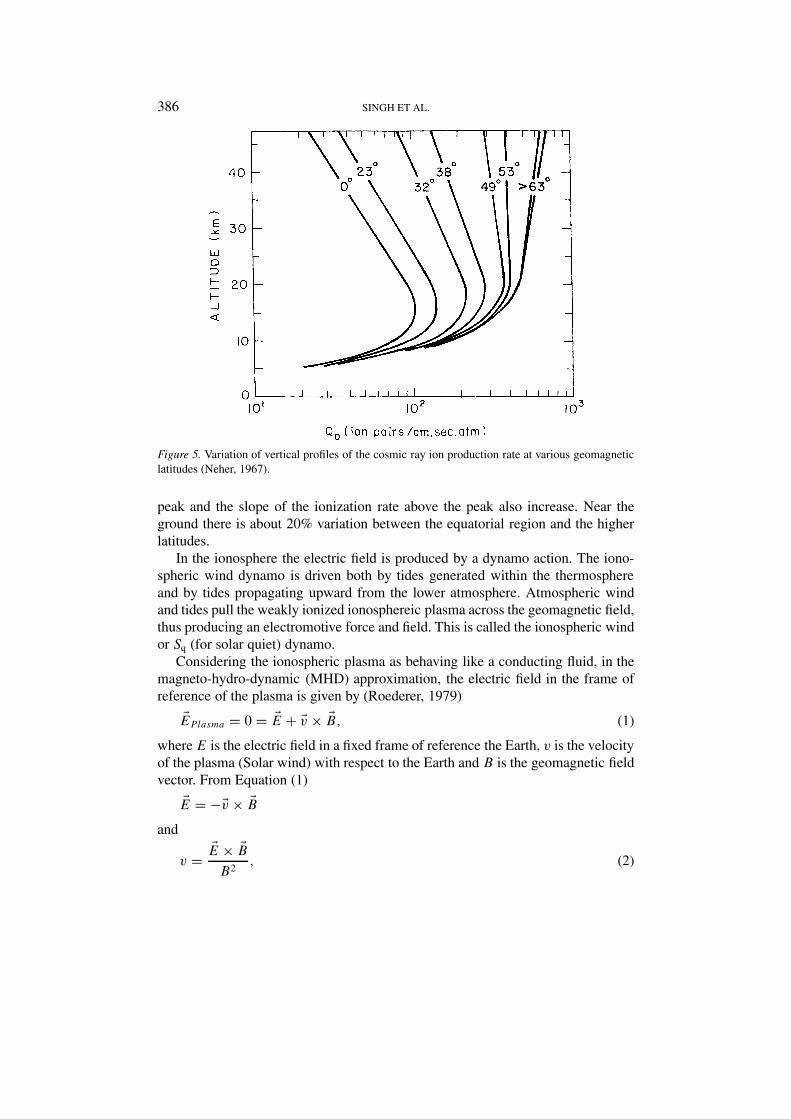
The electrical condition of the atmosphere depends upon its state of ionization.The main source of the ionization up to the altitude of 60 km is Galactic cosmicrays, although additional ionization near the ground can be produced by radioactiveemissions from the ground and owing to release of radioactive gases from thesoil, and above 60 km solar ultraviolet radiation becomes important. During thegeomagnetic storm period energetic auroral electron precipitation, auroral X-raybremsstrahlung radiation, and proton bombardment during solar proton events, allcan become significant sources of additional ionization for the high latitude middleatmosphere. The full cosmic ray spectrum is only capable of reaching the Earth’ssurface at geomagnetic latitudes higher than ∼ 60◦. At lower geomagnetic latitudesthe lower energy particles are successively excluded by the Earth’s geomagneticfield, and only particles with energies greater than about the 15 GeV range canreach the equator. The cosmic ray spectrum thus hardens with decrease in geomag-netic latitude. As a result the height of the maximum ion production rate decreasesfrom about 20 km at mid latitudes to about 15 km near the equator. The profile ofthe ion production rate for cosmic rays for various geomagnetic latitudes duringthe solar cycle minimum, using the data from Neher (1967), is shown in Figure 5.The ionization rate increases with geomagnetic latitude, and both the height of the

386 SINGH ET AL.

Figure 5. Variation of vertical profiles of the cosmic ray ion production rate at various geomagneticlatitudes (Neher, 1967).

peak and the slope of the ionization rate above the peak also increase. Near theground there is about 20% variation between the equatorial region and the higherlatitudes.

In the ionosphere the electric field is produced by a dynamo action. The iono-spheric wind dynamo is driven both by tides generated within the thermosphereand by tides propagating upward from the lower atmosphere. Atmospheric windand tides pull the weakly ionized ionosphereic plasma across the geomagnetic field,thus producing an electromotive force and field. This is called the ionospheric windor Sq (for solar quiet) dynamo.

Considering the ionospheric plasma as behaving like a conducting fluid, in themagneto-hydro-dynamic (MHD) approximation, the electric field in the frame ofreference of the plasma is given by (Roederer, 1979)

�EPlasma = 0 = �E + �v × �B, (1)

where E is the electric field in a fixed frame of reference the Earth, v is the velocityof the plasma (Solar wind) with respect to the Earth and B is the geomagnetic fieldvector. From Equation (1)

�E = −�v × �Band

v = �E × �BB2

, (2)


Equation (2) shows the inter-relationship between the electric field and plasmavelocity. The MHD approximation is useful in inter-relating plasma motions withthe electric and magnetic field, but it breaks down in a number of important circum-stances, especially where electric current densities are large. It also breaks down inthe lower ionosphere, below 150 km, where collisions between ions and the muchmore numerous neutrals (air molecules) are sufficiently frequent to prevent theions from maintaining the velocity given by the Equation (2). In this region electriccurrent readily flows across geomagnetic field lines. The winds in neutral air windsin the lower ionosphere lead to the generation of electric currents and fields, andfor this reason the height range of roughly 90–150 km is called the dynamo regionof the ionosphere.

Volland (1972, 1977) has shown that the large scale horizontal potential differ-ence generated in the ionosphere by the wind dynamo maps downward into thelower atmosphere and perturbs the low latitude potential and electric field near theground by about 1–5% of the tropospheric fair weather potential and electric fieldstabilized by worldwide thunderstorm activity. During the geomagnetic stormsperiod thermospheric winds acting in response to heating by high latitude auroralactivity produce an ionospheric disturbance dynamo, and large scale horizontalpotential differences of up to 25 kV are generated between high and low latit-udes by the ionospheric disturbance dynamo (Blanc and Richmond, 1980). Thesedisturbances are superimposed on the quiet ionospheric wind dynamo potentials.Muhleisen et al. (1971) showed that the ionospheric potential difference inferredfrom measurements made at widely separated mid and low latitude stations isgenerally small, although during one strong event they found a 60 kV ionosphericpotential difference between two stations.

The solar wind/magnetosphere dynamo is driven by the interaction of solarwind with the Earth’s geomagnetic field. It generates a horizontal dawn to duskpotential drop of 30–150 kV across magnetic conjugate points in polar caps, and itis associated with a current system which carries current of the order of 106 A. Themagnetospheric convection pattern is aligned to the Sun relative to the geomagneticpoles (north geomagnetic pole, 78.3 ◦N latitude and 291◦E longitude; south geo-magnetic pole, latitude 74.5 ◦S and longitude 127 ◦E). The pattern remains fixedrelative to the Sun and moves in a complex fashion over the Earth’s surface as theEarth rotates about its geographical polar axis. Solar wind/magnetosphere dynamois the major generator of electric fields in the magnetosphere, and the electric fieldis given by

�E = �Vsw × �B, (3)

where �Vsw is the solar wind velocity. The source of this electric field can be ap-preciated by considering the magnetosphere as a MHD generator in which a jetof plasma is forced through a static magnetic field and an electric potential is de-veloped by dynamo action. If the magnetosphere were static the solar wind wouldblow across the field lines and an electric field would be generated. The magnitude

388 SINGH ET AL.

Figure 6. Schematic diagram of Earth’s magnetic field and plasma flow in the solar wind/ magneto-sphere. Solid lines show the magnetic field, open arrows show the plasma velocity’s direction. a, b,c, and d denote magnetic regions of different topology (Lyons and Williams, 1984).

of this field is just that required to produce the circulation. The total potential dropis given by

VT = VswLBn, (4)

where L is the width of the magnetosphere and Bn is estimated from the magneticflux leaving the polar caps which ultimately connects to the IMF. For a polar capof radius Rp and magnetic flux density Bp, a magnetotail of length ST and radiusRT (= L/2), (Hargreaves, 1992).

Bn = πR2PB2

P

2πRT ST

, (5)

Taking RP = 1.7 × 106 m, BP = 5.5 × 10−5 Wbm−2, RT = 20 RE, and ST =200 RE, one obtains Bn = 4.5 × 10−10 Wbm−2 ∼ 0.45 nT. A solar wind speed ofVsw = 500 km/sec gives VT = 58 kV. Although this calculation assumes valueswhich may not be well known, it does give a result of the right magnitude, and,so reinforces the validity of the electric potential approach. Furthermore, it is oftenmore convenient to treat the dynamics of the magnetosphere in terms of the electricfield.

The electric potential developed during the dynamo process depends on theorientation of the Earth’s magnetic field which extends indefinitely into interplan-etary space (Hill and Wolf, 1977; Stern, 1977; Lyons and Williams, 1984). Forready reference we present a schematic diagram of the magnetic field configuration(Figure 6) where the IMF is directed southward. If the IMF had an east - westcomponent, as it usually does, we would require a three-dimensional representation


of the magnetic field configuration which is very complex. In fact, Figure 6 repres-ents a conceptual tool rather than a true representation of the magnetospheric fieldlines. In the figure there are four classes of magnetic field lines shown: (a) closedmagnetic field lines connected to the Earth in both northern and southern hemi-sphere; (b) interplanetary field lines unconnected to the Earth; (c) open field linesconnecting the northern polar cap to interplanetary space; and (d) open field linesconnecting the southern polar cap to interplanetary space. The interplanetary elec-tric field, obtained from (2), is directed out of the paper in Figure 6. To the extentthat the MHD approximation is valid and electric fields map along the magneticfield, the polar ionosphere is also subjected to an electric field out of the paper,causing ionospheric plasma to convect anti-sunward. The ionospheric electric fieldis greater than that of the interplanetary electric field because the bending of mag-netic field lines at the ionosphere causes electric potential gradients to intensify.On the other hand, the drift velocity of the plasma in the upper ionosphere is muchlower than the solar wind velocity because of the inverse dependence on magneticfield strength. The polar cap electric field is 20 mV/m, giving an ionospheric con-vection velocity of roughly 300 m/sec. The physical processes that determines theamount of magnetic flux that interconnect the geomagnetic field and the IMF arenot well understood (Cowely, 1982). It involves violation of the MHD approxim-ation, which occurs to some extent through the magnetosphere, but is particularlyimportant in at least two regions: at the sunward the magnetopause and somewherein the magnetospheric tail. In the sunward direction the magnetopause plasmaflows together through unconnected interplanetary and magnetospheric magneticfields and flows out northward and southward on interconnected magnetic fieldlines. In the tail the plasma flows together on interconnected field lines and flowsout through unconnected magnetospheric and IMF. In the closed portion of themagnetosphere the plasma flows generally towards the sun, passing around theEarth on the morning and evening side. However, some of the outermost portion ofthe cloud field region convects away from the sun because of momentum transferfrom the nearby solar wind (Hones, 1983).

The magnetospheric plasma convection causes energization of plasma andparticle precipitation into the ionosphere and hence affects the electrodynamicproperties of the ionosphere. The convection of plasma from the magnetosphere tothe ionosphere is compressionally heated because the volume occupied by plasmaon neighboring magnetic field lines is reduced as magnetic field strength increases.Other processes also help in the energization of the plasma. Some of the energizedparticles precipitate into the ionosphere as a result of wave - particle interactionand create ionization enhancements, especially in the auroral oval (Tsurutani andLakhina, 1997; Singh and Singh, 2002; Singh et al., 2003). The energized plasmaalso has an important influence on the flow of the electric currents and on thedistribution of electric fields (Spiro and Wolf, 1984). Energetic particles drift inthe Earth’s magnetic field, electrons towards the east and positive ions towards thewest, so that a westward ring current flows within the hot plasma. This current

390 SINGH ET AL.

flowing in the geomagnetic field essentially exerts an electromagnetic force on theplasma directed away from the Earth; thus tending to oppose the Earthward convec-tion. Charge separation associated with the ring current tends to create an eastwardelectric field component, opposite to the nightside westward convection electricfield, largely canceling the convection electric field in the inner magnetosphere.The overall pattern of magnetospheric convection tends to map along the magneticfield line into the ionosphere, even though this mapping is imperfect because of thenet electric field which tends to develop within the non-uniform energetic plasma.In the upper ionosphere, where (2) is valid, the general convection pattern looks asshown in Figure (7). The flow lines in Figure (7) correspond to lines of constantelectrostatic potential in a steady state. There is a potential high on the dawn sideof the polar cap and low on the dusk side, with a potential difference of the orderof 50 kV. The electric field strength in the auroral oval tends to be somewhat largerthan the polar cap electric field.

We have tried to show above that the electrical properties of different regionsare linked and that one is not justified in studying the electrodynamics of theEarth’s atmosphere region by region, i.e., separately for troposphere, stratosphere,mesosphere, ionosphere, magnetosphere, and interplanetary medium. The electricfield and current map from one region to the other, and control the electrodynamicproperties of the entire atmosphere. Therefore a global approach is required inorder to understand the electrical environment of the Earth’s atmosphere (Lakhina,1993).

4. Global Electric Circuit

The concept of a GEC began to evolve in the early twentieth century with the re-cognition of the following facts: (a) the net positive space charge in the atmospherebetween the Earth’s surface and a height of ∼ 10 km is nearly equal to the negativecharge on the Earth’s surface; (b) the electrical conductivity of the air increaseswith altitude and the air – earth current within an atmospheric column remainsconstant with altitude, which implies that this is being driven by a constant voltagedrop between the surface of the Earth and upper atmosphere. The discovery ofthe ionosphere during the same period provided the means of closing the globalcircuit through this conducting layer and played an important role in framing theconcept of the GEC. According to the classical picture of atmospheric electricitythe totality of thunderstorms acting together at any time charges the ionosphere toa potential of several hundred thousand volts with respect to the Earth’s surface(Dolezalek, 1972). This potential difference drives a vertical current downwardfrom the ionosphere to the ground in all fair weather regions of the globe. Thefair weather electric conduction current varies according to the ionospheric po-tential difference and the columnar resistance between the ionosphere and theground. The fair weather electric field varies typically between 100–300 V/m at


Figure 7. Schematic diagram of the magnetic north pole region showing the auroral oval andionospheric convection. The convection contours also represent electric potential contours, with apotential difference of the order of 8 kV between them (Burch, J.A.: 1977, ’The Magnetosphere,Upper Atmosphere and Magnetosphere, NRC Geophysics Study Committee, National Academy ofScience, Washington, DC, pp. 42–56).

the ground surface and shows diurnal, seasonal, and other time variations causedby many factors. The fair weather conductivity of the atmosphere near the Earth’ssurface is of the order of 10−14 mho/m and shows considerable variations withparticulate pollution (Cobb and Wells, 1970; Kamra and Deshpande, 1995; Kamraet al. 2001), relative humidity (Kamra et al., 1997), and radioactivity of the airand ground surface (Israelsson and Knudsen, 1986; Israelsson et al., 1987). Theelectric conductivity increases nearly exponentially with altitude up to 60 km withthe scale length of 7 km (Figure 2). This conductivity is maintained primarily bygalactic cosmic rays ionization. These Galactic cosmic rays flux reduces in the midlatitudes, when the solar activity increases, thus reducing the atmospheric conduct-ivity in this region, while in the same period solar protons may be ‘funnelled’ bythe Earth’s magnetic field to polar regions resulting in an increased atmosphericconductivity there. A dawn to dusk potential difference is also applied across thepolar regions as a result of the interaction of solar wind and the Earth’s magneticfield (Tinsley and Heelis, 1993). Cho and Rycroft (1998) have presented a simple

392 SINGH ET AL.

model profile for the atmospheric conductivity ranging from 10−13 mho/m nearthe surface to 10−7 mho/m at 80 km altitude in the lower ionosphere. Hale (1994)has presented a more complex profile, which shows variations in both space andtime. He has shown that the conductivity is three orders of magnitude higher at theheight of 35 km compared to that at the Earth’s surface, whereas the air density at35 km is 1% of the Earth’s surface. Below 60 km the main charge carriers are smallpositive and negative ions which are produced primarily by galactic cosmic rays,and above 60 km free electrons become more important as charge carriers, andtheir high mobility abruptly increases the conductivity throughout the mesosphere.However, near the Earth’s surface the conductivity is large enough to dissipateany field in just 5–40 min (depending on the amount of pollution); therefore thelocal electric field must be maintained by some almost continuous current source.Above 80 km the conductivity becomes anisotropic because of the influence ofthe geomagnetic field and shows diurnal variation owed to solar photo-ionizationprocesses. The arena for the subject is included in the system shown in Figure 8which shows the Earth at the center, surrounded by the atmosphere, ionosphere, theVan Allen belts, and the magnetosphere deformed by the solar wind coming fromthe Sun. During the geomagnetically active periods the energetic charged particlesprecipitating from the Earth’s inner and outer magnetospheric radiation belts (Fig-ure 8) interact with the middle and lower atmosphere by depositing their energyin the atmosphere, by creating ionization directly or via bremmstrahlung radiation,by altering its chemistry (Jackman et al., 1995), or by affecting the nucleation byelectrofreezing of water droplets to form clouds, thereby influencing the dynamicsof storm, and the atmosphere (Tinsley and Heelis, 1993; Tinsley, 1996, 2000). Thusthe electrical behaviour of the Earth’s environment is controlled by the dynamicsof the solar atmosphere.

The Earth’s surface and the ionosphere provide two conducting plates wherecurrent flows horizontally. Figure 4 shows that the GEC is driven by the upwardcurrent from a thunderstorm’s top towards the ionosphere and also from the groundinto the thunderstorm generators, thus closing the circuit (Markson, 1978). Theglobal fair weather load resistance is of the order of 100 �. About 2000 thunder-storms occurring around the globe at any one time are the source of current (theWilson current) in the circuit (Figure 3). They occur mostly in the tropics in thelocal afternoon and evening. Aircraft and balloon measurements above thunder-storms show that a total current of 0.1–6 A, with an average of 0.4 A, flows fromthe top of a thunderstorm cell to the ionosphere (Gish and Wait, 1950; Stergis et al.,1957; Vonnegut et al., 1973; Kasemir, 1979). Below a thunderstorm the transfer ofcharge by point discharge, lightning, precipitation, convection and displacementcurrents contributes to the net current flowing between the thunderstorm’s baseand the ground. Blakeslee et al. (1989) carried out measurements of air conduct-ivity and vertical electric field with a high altitude NASA U2 airplane flying overthunderstorms in the Tennessee valley region of the United States and reported thatthe Wilson current varied from 0.09–3.7 A with an average of 1.7 A, and the area-


Figure 8. Schematic diagram of Earth’s magnetosphere, showing the Earth at the center, surroundedby the atmosphere, the ionosphere, the Van Allen radiation, and the magnetosphere deformed by theflowing solar wind (Davies, K., Ionospheric Radio, Peter Peregrinus, London, 1990).

averaged Maxwell current varied from 0.09–5.9 A with an average of 2.2 A. Theyhave also shown that the relative efficiency of a thunderstorm to supply currentto the GEC is inversely related to the storm flash rate. Thus the current generatedwithin the cloud is divided between production of lightning and maintenance ofthe Wilson current. Intra-cloud discharges do not support the Wilson current. Theratio of cloud to ground and intra-cloud discharge increases from about 0.1 in theequatorial region to about 0.4 near latitude 50◦ (Pierce, 1970; Prentice and Macher-ras, 1977). Thunderstorm activity is maximum near the equator and decreases withlatitude. Thus the supply of Wilson current varies with latitude and shows a peakat low latitudes.

Using the global model of atmospheric electricity Roble and Hays (1979) com-puted the electric field and air earth current density along the Earth’s orographicsurface which is shown in Figure 9. They present variation of the calculated elec-tric field and the air earth current density over the Earth’s surface caused by thedownward mapping of the magnetospheric convection potential pattern. Underthe maximum positive ionospheric potential, the calculated surface electric fieldis +15 V/m (positive ionospheric potential regions; the air – earth current flows

394 SINGH ET AL.

Figure 9. Contours illustrating the downward mapping of the ionospheric potential pattern: (a) im-posed ionospheric potential (kV) at ionospheric height (> 100 km); (b) calculated electric field (V/M)along the Earth’s orographic surface; and (c) calculated ground current (A/m2, multiplied by 10−13)along the Earth’s orograpic surface. All figures are plotted at 19:00 UT in geomagnetic coordinates(Roble, and Hays, 1979).


into the ground) and under the minimum negative potential the calculated surfaceelectric field is −20 V/m (a negative ionospheric potential; the current flows fromthe ground towards the ionosphere). The maximum ground current density occursover the mountainous regions of Antarctica, Greenland and the Northern RockyMountains. The calculated air earth current shows considerable variations as aresult of the Earth’s orography that are associated with changes in the columnarresistance. In the vicinity of the high Antarctic mountain plateau the air earthcurrent has positive perturbations of up to 0.2 × 10−12 A/m2 on the dawn sideand to −2 × 10−12 A/m2 on the dusk side. This potential pattern moves overthe Earth’s surface during the day, rotating about the geomagnetic pole. Robleand Hays (1979) showed that in sun-aligned geomagnetic coordinates at a groundstation, balloon, or aircraft at a given geographic location should detect variationsthat are organized in magnetic local time. At an early magnetic local time the iono-spheric potential perturbations of the Earth’s potential gradient are positive, andat a later magnetic local time negative potential overtakes times and the perturba-tions are negative. Owing to orographic variations the globally integrated groundcurrent varies between net upward and downward values, which in turn causesthe difference in the fair weather ionospheric potential to vary between positiveand negative values in a diurnal cycle (Roble and Hays, 1979). Analyzing the datarecorded at the South Pole and Thule, Greenland, Kasemir (1972) showed that thediurnal Universal time (UT) variations of potential gradient are about 30% lessthan the global low latitude UT variations, which are attributed to variations inthunderstorm frequency. The polar curve has a similar shape to the curve derivedfrom the Carnegie cruise, but at a much reduced amplitude. From these resultsKasemir (1979) concluded that another agent, besides worldwide thunderstormactivity, may modulate the global circuit at high latitudes. Kamra et al. (1994)have challenged the concept of the classical GEC on the basis of their electricfield observations in the Indian Oceans. Recent observations of Deshpande andKamra (2001) also show that diurnal variation of the electric field at Antarcticasignificantly differs from the Carnegie diurnal curve of the electric field.

Analyzing the balloon measurements of magnetospheric convection fields dataMozer and Serlin (1969), Mozer (1971), Holzworth and Mozer (1979), Holzworth(1981), and D’Angelo et al. (1982) have studied the correlation of the verticalelectric field with the magnetic activity parameters. During quiet geomagneticconditions the classical Carnegie curve could be reproduced at the location of theballoon’s height, and during more active geomagnetic conditions the dawn – duskpotential difference of the magnetospheric convection pattern was found to clearlyinfluence the vertical fair weather field as it intensified and presumably moved fromits quiet time position to over the balloon’s height. Measurements of the verticalelectric field at Syowa station (Antarctica) showed that it increases in response toa magnetospheric substorm (Tanaka et al., 1977). All these measurements sugges-ted an electrical coupling between the magnetospheric dynamo and the GEC at

396 SINGH ET AL.

Figure 10. A simplified equivalent circuit for the global electric circuit showing the thunderstorm asthe main generator (Ogawa, 1985).

high latitudes and indicated a need for more measurements in order to gain betterunderstanding of the nature of the interaction.

Only a few mathematical models of global atmospheric electricity have ap-peared over the years (Kasemir, 1963, 1977; Hill, 1971; Hays and Roble,1979;Volland, 1982; Ogawa, 1985). The widely referred model of Ogawa (1985), consid-ering the simple equivalent circuit for the atmosphere and an equipotential surfacefor the ionosphere, is shown in Figure 10. The thundercloud is treated as a constantcurrent generator with a positive charge at the top and negative charge at its bottom.Here r is the global resistance between the Earth and the ionosphere and R1, R2

and R3 are the resistances between the ionosphere and top of the thundercloud,between two charge centers within the thundercloud and between the bottom neg-ative charge and the Earth’s surface, respectively. Since R1, R2, and R3 are muchgreater than r, the upward current from the thundercloud to the ionosphere is givenby

I = R2I0

R1 + R2 + R3(6)

It should the noted that the current I is also the fair weather current from theionosphere to the Earth’s surface and it is related to the thunderstorm generatorcurrent I0. The measurement of I at a high altitude observatory remote from activethunderstorms can give some information about I0, if R1 and R2 are considered asconstant. Both may, however, be reduced at times of enhanced fluxes of energeticcharged particles associated with enhanced geomagnetic activity. The contributionto R1 above an active, sprite-producing thundercloud may be greatly reduced owingto ionization produced in the rarefied mesosphere by the large transient electricfield during large, positive cloud to ground lightning discharges (Cho and Rycroft,


Figure 11. The equivalent global electric circuit showing typical numerical values (Rycroft et al.,2000).

1998). Recent observations of optical emission between the top of the thunder-storm and the ionosphere suggest the existence of intense current which may be anextension of the return stroke current (Cummer et al., 1998; Cummer, 2003). Thiscurrent should be included in the mathematical modeling of GEC. Recently Paskoet al. (2002) have reported a video recording of a blue jet propagating upwards froma small thunder cloud cell to an altitude of about 70 km. As relatively small thundercloud cells are very common in the tropics, it is probable that optical phenomenafrom the top of the clouds may constitute an important component of the GEC.

Rycroft et al. (2000) presented a new model of GEC treating the ionosphereand the magnetosphere as passive elements (Figure 11). Three different regionsof the fair weather circuit are given. One of these is for the high altitude part ofthe Earth where the profiles of J and E through the fair weather atmosphere willdiffer from those of low and mid latitudes. The capacitance C of the concentricshell of atmosphere between the Earth and the ionosphere, over one scale height ofatmosphere rather than over the full height of the ionosphere, is

C = 4πε0R2e

H≈ 0.7 F, (7)

where Re is the radius of the Earth, ε0 the permittivity of free space, and H is thescale height which is equal to 7 km. The time constant for the atmospheric GEC

398 SINGH ET AL.

is τ = Cr ≈ 2 min (Rycroft et al., 2000). The energy associated with the globalelectric circuit is enormous, ≈ 2×1010 J (Rycroft et al., 2000). This value has beenobtained by considering a charge of 200 C associated with each storm and 1,000storms operating at a time. The electric current density through the fair weatheratmosphere ≈ 2 × 10−12 A/m−2. Taking the conductivity of air at ground levelto be ≈ 2 × 10−14 mho/m, the fair weather electric field is ≈ 102 V/m at groundlevel, ≈ 1 V/m at altitude 20 km and ≈ 10−2 V/m at altitude 50 km (Rycroft et al.,2000). Thus even though the fair weather current remains the same, the verticalelectric field goes on decreasing with altitude. The current remaining the same ifthe atmosphere conductivity changes owing to some reason, then accordingly thefair weather electric field also changes. For example, following a Forbush decrease,if the atmospheric conductivity is everywhere reduced by 10% then the fair weatherelectric field will be increased by ∼ 10% (Ogawa, 1985). The ionospheric potentialwould reduce to 99% of the initial value only for a few milliseconds after sprites,and would have little effect on the fair weather electric field (Rycroft et al., 2000).

Is there any affect of sprites on the global electric circuit? This is a completelyunanswered question to this date. A sprite occurs over large convective thunder-storms and affects the conductivity of the upper atmosphere (Rycroft and Cho,1998; Rycroft et al., 2000; Singh et al., 2002). The frequency of occurrence ofsprits is far less than that of lightning (only 1 sprite out of ∼ 200 lightning dis-charges). Based on such observations Rycroft et al. (2000) have suggested thatsprites do not play any major role in the GEC. However, intensive research intothis topic is required in future.

In all GEC models electrostatic phenomena have been considered, whereas dur-ing lightning discharges electromagnetic waves having frequencies from a few Hzto 100 MHz are generated and propagated through the atmosphere. To accountfor the effect of these waves electrodynamic or electromagnetic effects should beconsidered by relating electromagnetic fields to charge and current densities ina time varying situation. At higher frequencies (ω � σ/ε0) the medium can beconsidered as a leaky dielectric whereas at lower frequencies (ω � σ/ε0) it can beconsidered as a conductor. Even in the absence of radiation displacement currentshould be considered. In fact, the Maxwell current shown in Figure 3 is by itsnature very variable, and not a great deal is known about it. Further studies of thistopic are required.

The GEC model has several advantages over the traditional methods, baseddirectly or indirectly on the solar heating mechanism put forward for explainingsolar – terrestrial – weather relationships. The main drawback of the solar heatingmechanism is that the solar constant variations are very small (< 0.1%). Secondly,they require efficient coupling from the thermosphere to the lower atmosphere,which in reality is rather weak. Thirdly, the solar heating mechanisms are too slow;they require at least several days before atmospheric dynamics would be affectedsignificantly. The GEC model by passes all these difficulties, at the same time itoffers a novel approach to understanding the electrical environment of our planet.


For example, a change of ionospheric potential caused by solar flares would rapidlyaffect electric field intensities all over the world. The state of ionization of thelower atmosphere is controlled by cosmic rays of both solar and galactic origins,which again depend upon solar activity. A slight change in the ionization over thecloud top can affect the electric field throughout the lower atmosphere. Theoreticalmodeling shows that a slight change in the initial background electric field duringcloud electrification can lead to an entirely different final voltage being developed(Sartor, 1980). This is because the Earth’s atmosphere is a highly nonlinear system.

The main source of electrical phenomena upon the Earth’s environment is thun-derstorm activity, which is affected by solar activity. Brooks (1934) analyzed world-wide data collected from 22 stations and suggested a positive correlation betweenthe frequency of thunderstorms and relative sun spot numbers (R). The correlationwas low at mid latitudes and increased both towards the equator and the pole.Stringfellow (1974) analyzed data collected in Britain between 1930 and 1973and found the correlation coefficient between lightning frequency and sun spotnumbers to be ∼ 0.8. Recently Schlegel et al. (2001) analyzed data from the Ger-man lightning detection system (BLIDS) and showed a significant correlation oflightning frequency with AP and R, and a significant anti-correlation with cosmicray flux. However, a similar analysis with data from the Austrian System (ALDIS)yielded inconclusive results, although the two observing regions are quite closeto each other. The difference in lightning activity can be understood in terms ofthe weather system. The operational region of the ALDIS system lies in the southand east of the Alps mountains and is dominated by the continental Mediterranenweather system, whereas the area of the BLIDS system is mostly within the in-fluence of the north Atlantic weather system (Schlegel et al., 2001). The solaractivity influences the lower D region (Volland, 1995) and Schumann resonance(Schlegel and Fullekrug, 1999), which in turn affect the electrical environment ofthe Earth. A modern detection system should be used to explore new aspects of theSun – thunderstorm/lightning relationship and its variation with solar/geophysicalindices.

Recently GEC has been being used as a tool for studying the Earth’s climateand changes in it (Price and Rind, 1990, 1994) because of its direct connectionwith lightning activity. The subject has been recently reviewed by Williams (2003).A close relationship has been shown between: (a) tropical surface temperature andmonthly variability of the Schumann Resonance (Williams, 1992); (b) ELF ob-servations in Antarctic/Greenland and global surface temperature (Fuellekrug andFraser-Smith, 1997); (c) diurnal surface temperature changes and the diurnal vari-ability of the GEC (Price, 1993); and (d) ionospheric potential and global/tropicalsurface temperature (Markson and Price, 1999). Reeve and Toumi (1999), usingsatellite data, showed agreement between global temperature and global lightningactivity. Aerosols in the atmospheric boundary layer and stratosphere have a stronginfluence on the electrical phenomenon in the atmosphere. Adlerman and Williams(1996) found large effects from several factors such as seasonal changes, variations

400 SINGH ET AL.

in mixed layer heights, variations in the production rates and anthropogenic aero-sols, and variations in surface wind speed on the seasonal variations of the GEC.These aerosol particles can even influence the charge generating mechanisms instorms and thus affect the charging currents in the GEC (Williams et al., 2002).Williams and Heckman (1993) concluded that the conduction currents other thanlightning is the dominant charging agent for the Earth’s surface. Recently Price(2000) extended this study and showed a close link between the variability ofupper troposphere water vapour (UTWV) and the variability of global lightningactivity. UTWV is closely linked to other phenomena such as tropical cirrus cloud,stratospheric water vapour, and tropospheric chemistry (Price, 2000; Price andAsfur, 2003). These examples suggest that by monitoring the GEC it is possibleto study the variability of surface temperature, tropical deep convection, rainfall,upper troposphere water vapour, and other important parameters which affect theglobal climate system.

5. Conclusions

We have summarized the electrical behavior of different regions of the Earth’senvironment. Sources of electric fields and the electrodynamic processes involvedin each region have been discussed briefly. It has been suggested that the GECmodel, if properly solved, is able to provide short term and long term variations inthe electrical processes of various regions and their inter-coupling. Possible causesof changes in the GEC are discussed and its role in monitoring the Earth’s climateis indicated.

Recently observed optical phenomena (sprite, blue jets, blue starter, etc.) betweenthe ionosphere and the cloud top produces transient plasma which affects the elec-trodynamics of the atmosphere, and it should be explored in detail. In fact, furtherresearch is needed to better understand the natural environment and its variability,so that future evolution may be predicated.

Acknowledgements

One of the authors (DKS) thanks V. Gopalakrishnan and S.D. Pawar for helpfuldiscussion during the preparation of the manuscript. We are grateful to the refereefor his constructive and valuable suggestions.

Glossary

ELF: Extremely low frequency electromagnetic radiation (3–300 Hz).Fair weather: Normal sunny weather without any precipitation, without any ap-preciable amount of low cloud, and with calm/low winds.


L-parameter: The equation of a geomagnetic field line is r = L cos2 φ, where r isthe geocentric distance from the center of the Earth, φ is the magnetic latitude. Theparameter is the distance in Earth radii (RE) from the center of Earth to the pointwhere a geomagnetic field line crosses the equator (φ). L is useful in identifyingfield lines and magnetic drift shells.Interplanetary magnetic field: The magnetic field resulting from the outwardtransport of the solar magnetic field by the expanding solar plasma is known asthe solar wind.Lightning: A discharge of atmospheric electricity accompanied by a vivid flashof light. During thunderstorms static electricity builds up within the clouds. Apositive charge builds up in the upper part of the cloud, while a large negativecharge builds up in the lower portion. When the difference between the positiveand negative charges becomes large the electrical charge jumps from one area toanother, creating a lightning bolt. Most lightning bolts are intra-cloud, but they canalso strike the ground.Magnetotail: In the anti-sunward direction the magnetosphere is extended into along tail, the basic form of the magnetotail in the plane containing the magneticpoles is shown in Figure 1. The flux density is about 20 in the tail lobes.Plasma: A fourth state of matter (in addition to solid, liquid, and gas) which ex-ists in space. In this state atoms are positively charged and share space with freenegatively charged electrons (but overall electrically neutral). Plasma can conductelectricity and interact strongly with electric and magnetic fields. The solar wind isactually hot plasma blowing from the Sun.Schumann resonance: Schumann resonances are the eigenfrequencies of the Earth– ionosphere cavity oscillations excited by global lightning activity, and lie in thefrequency range 6–50 Hz.Solar cycle: Eleven year cycle of sunspots and solar flares that affects other solarindexes such as the solar output of ultraviolet radiation and the solar wind. TheEarth’s magnetic field, temperature, and ozone levels are affected by this cycle.Solar flare: A solar flare is a sudden brightening of the small area of the photo-sphere that may last between a few minutes and several hours.Solar wind: A plasma of protons and electrons, with an admixture of He++ andother lesser solar ions, streaming continuously together with the solar magneticfield from the solar atmosphere out to the solar system at a speed of ∼ 200–1000 km/s.Substorm: Basic disturbance in the terrestrial magnetosphere, involving success-ive reconfiguration of the geomagnetic field and explosive dissipation of energy inthe high latitude ionosphere (auroral displays), the inner plasma sheet (accelerationof energetic ions) and the distant magnetotail (formation of magnetic neutral linesand plasmoids). The energy is provided by the solar wind and is temporarily storedin the form of increased magnetic flux in the magnetotail.Sunspot: A region on the surface (the photosphere) of the Sun that is temporarilycool and dark compared to surrounding areas.

402 SINGH ET AL.

Thermosphere: High temperature (T > 1000 ◦K) region of the upper atmosphereabove 100 km.Thunderstorm: Local storm resulting from warm humid air rising in an unstableenvironment. Air may start moving upward because of unequal surface heating,the lifting of warm air along a frontal zone, or diverging upper level winds (thesediverging winds draw air up beneath them). Severe thunderstorms can producelarge hail, very strong winds, flash floods, and tornados.Wave - particle Interaction: Interactions between waves and particles in a plasmathat result in the exchange of energy and momentum and can result in whistler-induced electron precipitation.

References

Adlerman, E.J. and Williams, E. R.: 1996, ‘Seasonal Variation of the Global Electric Circuit’, J.Geophys. Res. 101, 29679–29688.

Barouch, E. and Burlaga, L. F.: 1975, ‘Causes of Forbush Decreases and Other Cosmic RayVariations’, J. Geophys. Res. 80, 449–456.

Barrington-Leigh, C. P. and Inan, U. S.: 1999, ‘Elves Triggered by Positive and Negative LightningDischarges’, Geophys. Res. Lett. 26, 683–686.

Barrington-Leigh, C. P., Inan, U. S., Stanley, M. and Cummer, S. A.: 1999, ‘Sprites Triggered byNegative Lightning Discharges’, Geophys. Res. Lett. 26, 3605–3608.

Bering, E. A., Rosenberg, T. J., Benbrook, J. R., Detrick, D., Muthews, D. L., Rycroft, M. J., SaundersM. A., and Sheldon, W. R.: 1980, ‘Electric Fields, Electron Precipitation and VLF Radio WaveDuring a Simultaneous Magnetospheric Substorm and Atmospheric Thunderstorm’, J. Geophys.Res. 85, 55–72.

Bering, E. A., Benbrook, J. R., Garrett, J. A., Paredes, A. M., Wescott, E. M., Moudry, D. R.,Sentman, D. D., and Stenbaek-Nielsen, H. C.: 2002, ‘The Electrodynamics of Sprites’, Geophys.Res. Lett. 29, 10.1029/2001GL013267.

Blakeslee, R. J., Christian H. J., and Vonnegut, B.: 1989, ‘Electrical Measurements over Thunder-storms’, J. Geophys. Res. 94, 13135–13140.

Blanc, N. and Richmond, A. D.: 1980, ‘The Ionosphere Disturbance Dynamic’, J. Geophys. Res. 85,1669–1686.

Boeck, W. L., Vaughan, Jr. O. H., Blakeslee, R. J., Vonnegut, B., Brook, M.: 1998, ‘The Role of theSpace Shuttle Video Tapes in the Discovery of Sprites’, J. Atmospheric Solar Terrest. Phys. 60,669–677.

Boys, C. V.: 1926, ‘Progressive Lightning’, Nature 118, 749–750.Brooks, C. E. P.: 1934, ‘The Variation of the Annual Frequency of Thunderstorm in Relation to

Sunspots’, Quart. J. Roy. Met. Soc. 60, 153–165.Cho, M. and Rycroft, M. J.: 1998, ‘Computer Simulation of Electric Field Structure and Optical

Emission from Cloud Top to Ionosphere’, J. Atmospheric Solar Terrest. Phys. 60, 871–888.Cobb, W. E.: 1967, ‘Evidence of a Solar Influence on the Atmospheric Electric Element at Mauna

Lao Observatory’, Monthly Weather Rev. 95, 905–911.Cobb, W. E. and Wells, H. J.: 1970, ‘The Electrical Conductivity of Oceanic Air and its Correlation

to Global Atmospheric Pollution’, J. Atmospheric Sci. 27, 814–819.Cowley, S. W. H.: 1982, ‘The Causes of Convection in the Earth’s Magnetosphere: A Review of

Development during the IMS’, Rev. Geophys. Space Phys. 20, 531–565.Cummer, S. A.: 2003, ‘Current Moment in Sprite-Producing Lightning’, J. Atmospheric Solar

Terrest. Phys. 65, 499–508.


Cummer, S. A., Inan, U. S., Bell, T. F., and Barrington-Leigh, C. P.: 1998, ‘ELF Radiation Producedby Electrical Currents in Sprites’, Geophys. Res. Lett. 25, 1281–1285.

D’Angelo, N., Iversen, I. B. and Madsen, M. M.: 1982, ‘Influence of the Dawn – Dusk PotentialDrop Across the Polar Cap on the High Latitude Atmospheric Vertical current’, Geophys. Res.Lett. 9, 773–776.

Deshpande, C. G. and Kamra, A. K.: 2001, ‘Diurnal Variations of the Atmospheric Electric Field andConductivity at Maitri, Antarctica’, J. Geophys. Res. 106, 14207–14218.

Dolezalek, H.: 1972, ‘Discussion the Fundamental Problem of Atmospheric Electricity’, Pure Appl.Geophys. 100, 8–43.

Duggal, S. P.: 1979, ‘Relativistic Solar Cosmic Rays’, Rev. Geophys. Space Phys. 17, 1021–1058.Duggal, S. P. and Pomerantz, M. A.: 1977, ‘The Origin of Transient Cosmic Ray Intensity

Variations’, J. Geophys. Res. 82, 2170–2174.Dungey, J. W.: 1978, ‘The History of the Magnetopause Region’, J. Atmospheric Terrest. Phys. 40,

231–234.Everett, J. D.: 1903, ‘Rocket Lightning’, Nature 68, 599.Franz, R. C., Nemzek, R. J. and Winckler, J. R.: 1990, ‘Television Image of a Large Upward Electrical

Discharge Above a Thunderstorm System’, Science 249, 48–51.Freier, G. D.: 1961, ‘Auroral effect on the Earth’s electric field’, J. Geophys. Res. 66, 2695–2702.Freier, G. D.: 1979, ‘Time-Dependent Field and a New Mode of Charge Generation in Severe

Thunderstorms’, J. Atmospheric Sci. 36, 1967–1975.Fuellekrug, M. and Fraser-Smith, A. C.: 1997, ‘Global Lightning and Climate Variability Inferred

from ELF Magnetic Field Variations’, Geophys. Res. Lett. 25, 2411–2414.Gish, O. H. and Wait, G. R.: 1950, ‘Thunderstorms and the Earth’s General Electrification’, J.

Geophys. Res. 55, 473–484.Gringel, W., Rosen, J. M. and Hofmann, D. J.: 1986, ‘Electrical Structure from 0 to 30 Kilomet-

ers’, Studies in Geophysics - The Earth’s electrical Environment, National Academy Press,Washington, D.C., pp. 166–182.

Hale, L. C.: 1994, ‘The Coupling of ELF/VLF Energy from Lightning and MeV Particle to theMiddle Atmosphere, Ionosphere and Global Circuit’, J. Geophys. Res. 99, 21089–21096.

Hargreaves, J. K.: 1992, The Solar-terrestrial Environment, University of Lancaster, University Press,Cambridge.

Hays, P. B. and Roble, R. G.: 1979, ‘A Quasi-Static Model of Global Atmospheric Electricity. 1. TheLower Atmosphere’, J. Geophys. Res. 84, 3291–3305.

Heaps, M. G.: 1978, ‘Parameterization of the Cosmic Rays Ion-Pair Production Rate above 18 km’,Planetary Space Sci. 26, 513–517.

Hill, R. D.: 1971, ‘Spherical Capcitor Hypothesis of the Earth’s Electric Field’, Pure Appl. Geophys.84, 67–75.

Hill, T. W. and Wolf, R. A.: 1977, ‘Solar Wind Interaction in the Upper Atmosphere and Magneto-sphere’, NRC Geophysics Study Committee, National Academy of Sciences, Washington, D.C,pp. 25–41.

Hines, C.: 1963, ‘The Magnetopause: A New Frontier in Space’, Science 141, 130–136.Hofmann, D. J. and Rosen, J. M.: 1979, ‘Balloon-Borne Measurements of Atmospheric Electrical

Parameters. I The Ionization Rate’, Atmospheric Phys. Rep. AP. 54, University of Wyoming,Laramie.

Holzworth, R. H.: 1981, ‘High Latitude Stratospheric Electric Measurements Infair and Foul Weatherunder Various Solar Conditions’, J. Atmospheric Terrest. Phys. 43, 1115–1126.

Holzworth, R. H. and Mozer, F. S.: 1979, ‘Direct Evidence of Solar Flare Modification StratosphericElectric Fields’, J. Geophys. Res. 84, 363–367.

Holzworth, R. H. and Hu, H.: 1995, ‘Global Electrodynamics from Superpressure Balloons’, Adv.Space Res. 16, 131–140.

Hones, E. W.: 1983, ‘Magnetic Structure of the Boundary Layer’, Space Sci. Rev. 34, 201–211.

404 SINGH ET AL.

Hoppel, W. A., Anderson, R. V. and Willett, J. C.: 1986, ‘Atmospheric Electricity in the PlanetaryBoundary Layer’, Study in Geophysics - The Earth electrical Environment, National AcademyPress, Washington, D.C., pp. 149–165.

Hu, H., Li., Q. and Holzworth, R. H.: 1989, ‘Thunderstorm Related Variations in StratosphericConductivity Measurements’, J. Geophys. Res. 94, 16429–16435.

Huang, E., Williams, E.R., Boldi, R, Heckman, S., Lyons, W., Taylor, M., Nelson, T., and Wong, C.:1999, ‘Criteria for Sprites and Elves Based on Schumann Resonance Observations’, J. Geophys.Res. 104, 16943–16964.

Israelsson, S. and Knudsen, E.: 1986, ‘Effect of Radioactive Fallout from a Nuclear Power PlantAccident on Electrical Parameters’, J. Geophys. Res. 91, 11909–11910.

Israelsson, S., Schutte, T., Pisler, E., and Lundquist, S.: 1987, ‘Increased Occurrence of LightningFlashes in Sweden During 1986’, J. Geophys. Res. 92, 10996–10998.

Jackman, C. H., Cerniglia, M. C., Nielsen, J. E., Allen, D. J., Zawodny, J. M., McPeters, R. D.,Douglass, A. R., Rosefield, J. E., and Rood, B.: 1995, ‘Two-Dimensional and Three-DimensionalModel Simulations, Measurements and Interpretation of the Influence of the October 1989 SolarProton Events on the Middle Atmosphere’, J. Geophys. Res. 100, 11641–11660.

Kamra, A. K. and Deshpande, C. G.: 1995, ‘Possible Secular Change and Land to Ocean Extensionof Air Pollution from Measurements of Atmospheric Electrical Conductivity over the Bay ofBangal’, J. Geophys. Res. 100, 7105–7110.

Kamra, A. K., Deshpande, C. G. and Gopalakrishnan, V.: 1994, ‘Challenge to the Assumption of theUnitary Diurnal Variation of the Atmospheric Electric Field Based on Observations in the IndianOcean, Bay of Bengal and the Arabian Sea’, J. Geophys. Res. 99, 21043–21050.

Kamra, A. K., Deshpande, C. G. and Gopalakrishnan, V.: 1997, ‘Effect of Relative Humidity on theElectrical Conductivity of Marine Air’, Quart. J. Roy. Meteorol. Soc. 123, 1295–1305.

Kamra, A. K., Murugavel, P., Pawar, S. D. and Gopalakrishnan, V.: 2001, ‘Background AerosolConcentration Derived from the Atmospheric Conductivity Measurements Made over the IndianOcean During INDOX’, J. Geophys. Res. 106, 28643–28651.

Kasemir, H. W.: 1963, ‘On the Theory of the Atmosphere Electric Current Flow’, IV Technical Re-port No. 2394, U.S Army Electronics Research and Development Laboratories Fort Monmouth ,N.J., October.

Kasemir, H. W.: 1972, ‘Atmospheric Electric Measurements in the Arctic and Antarctic’, Pure Appl.Geophys. 100, 70–80.

Kasemir, H. W.: 1977, ‘Theoretical Problem of the Global Atmospheric Electric Current’, ElectricalProcesses in Atmospheres, in H. Dolezalek, and R. Reiter (eds), Steinkopff Verlag, Darmstadt,pp. 423–438.

Kasemir, H. W.: 1979, ‘The Atmospheric Electric Global Circuit’, Proceedings of Workshop on theNeed for Lightning Observations from Space, NASA, CP-2095 pp. 136–147.

Krehbiel, R. R., Brook, M. and McCrosy, R. A.: 1979, ‘An Analysis of Charge Structure of LightningDischarge to Ground’, J. Geophys. Res. 84, 2432–2466.

Krider, E. and Musser, J. A.: 1982, ‘The Maxwell Current Density under Thunderstorm’, J. Geophys.Res. 87, 11171–11176.

Lakhina, G. S.: 1993, ‘Electrodynamic Coupling Between Different Regions of the Atmosphere’,Curr. Sci. 64, 660–666.

Lobodin, T. V. and Paramonov, N. A.: 1972, ‘Variation of Atmospheric Electric Field DuringAurorae’, J. Pure. Appl. Geophys. 100, 167–173.

Lyons, W. A.: 1994, ‘Characteristics of Luminous Structures in the Stratosphere Above Thunder-storms as Imaged by Low–Light Video’, Geophys. Res. Lett. 21, 875–878.

Lyons, L. R. and Williams, D. J.: 1984, Quantitative Aspects of Magnetospheric Physics, D. ReidelPublishing Co., Dordrecht, Holland.

Malan, D. J.: 1937, Physics of Lightning (English), Acad. Science, Paris.


Marcz, F.: 1976, ‘Links Between Atmospheric Electricity and Ionospheric Absorption due to ExtraTerrestrial Influences’, J. Geophys. Res. 81, 4566–4570.

Markson, R.: 1971, ‘Consideration Regarding Solar and Lunar Modulation of Geophysical Paramet-ers, Atmospheric Electricity and Thunderstorm’, Pure Appl. Geophys. 84, 161–202.

Markson, R.: 1978, ‘Solar Modulation of Atmospheric Electrification and Possible Implication forthe Sun-Weather Relationship’, Nature 273, 103–105.

Markson, R. and Muir, M.: 1980, ‘Solar Wind Control of the Earth’s Electric Field’, Science 208,979–990.

Markson, R. and Price, C.: 1999, ‘Ionospheric Potential as a Proxy Index for Global Temperatures,Atmospheric Res. 51, 309–314.

Meyerott, R. E., Reagan, J. B. and Evans, J. E.: 1983, Weather Climate Responses to Solar Variation,B.M. McCormae (ed), Colorade, Associated University Press, Boulder.

Michnowski, S.: 1998, ‘Solar Wind Influences on Atmospheric Electrical Variables in PolarRegions’, J. Geophys. Res. 103, 13939–13948.

Mozer, F. S.: 1971, ‘Balloon Measurement of Vertical and Horizontal Atmosphereic Electric Fields’,Pure Appl. Geophys. 84, 32–45.

Mozer, F. S. and Serlin, R.: 1969, ‘Magnetospheric Electric Fields Measurements with Balloons’, J.Geophys. Res. 74, 4739–4754.

Muhleisen, R.: 1971, Neue Ergebniss und Problem in der Luftelektrezutat, z. Geophys. 37, 759–793.Muhleisen, R.: 1977, ‘The Global Circuit and its Parameters’, Electrical Process in Atmospheres, H.

Dolezalek and R. Reiter (eds), Steinkoff, Darmstadt, Germany.Muhleisen, R., Fisher, H. J. and Hofmann, H.: 1971, ‘Horizontal Electric Fields in the Ionospher

Derived from Air Electric Measurements’, J. Geophys. Res. 37, 1055–1059.Nagano, I., Yagitani, S., Migamura, K., and Makino, S.: 2003, ‘Full Wave Analysis of Elves Created

by Lightning-Generated Electromagnetic Pulses’, J. Atmospheric Solar Terrest. Phys. 65, 615–625.

Neher, H. V.: 1967, ‘Cosmic Rays Particle that Changed from 1954 to 1958 to 1965’, J. Geophys.Res. 72, 1527–1539.

Nickolaenko, A. P. and Hayakawa, M.: 1998, ‘Electric Fields Produced by Lightning Discharges’, J.Geophys. Res. 103, 17175–17189.

Ogawa, T.: 1985, ‘Fair Weather Electricity’, J. Geophys. Res. 90, 5951–5960.Olson, D. E.: 1971, ‘The Evidence for Auroral Effects on Atmospheric Electricity’, Pure Appl.

Geophys. 84, 118–138.Olson, D. E.: 1977, ‘Influence of Solar Activity and Geomagnetic Changes on Weather and Climate’,

IAGA/IAMAP Joint Assembly, Seattle, Washington.Park, C. G.: 1976, ‘Solar Magnetic Sector Effects on the Vertical Atmospheric Electric Field at

Vostok, Antarctica’, Geophys. Res. Lett. 3, 475–478.Pasko, V. P., Inan, U. S., Taranenko, Y. N., and Bell, T. F.: 1995, ‘Heating, Ionization and Upward

Discharges in the Mesosphere due to Intense Quasi-Electrostatic Thundercloud Fields’, Geophys.Res. Lett. 22, 365–368.

Pasko, V. P., Inan, U. S., Bell, T. F. and Taranenko, Y. N.: 1997, ‘Sprites Produced by Quasi-Electrostatic Heating and Ionization in the Lower Ionosphere’, J. Geophys. Res. 102, 4529–4561,

Pasko, V. P., Stanley, M. A., Mathews, J. D., Inan U. S. and Wood, T. G.: 2002, ‘Electrical Dischargefrom a Thundercloud Top to the Ionosphere’, Nature 416, 152–154.

Pierce, E. T.: 1970, ‘Latitudinal Variation of Lighting Parameters’, J. Appl. Meteorology 9, 194–195.Pierce, E. T. and Whitson, A. L.: 1965, ‘Atmospheric Electricity and Waterfalls of Yosemite Valley’,

J. Atmospheric Sci. 22, 314–319.Pinto, I. R. C. A., Pinto, O., Gonzalez, W. D., Dutra, S. L. G., Wygant, J. and Mozer, F. S.: 1988,

‘Stratosheric Electric Fields and Conductivity Measurements over Electrifield Cloud in the SouthAmerican Region’, J. Geophys. Res. 93, 709–715.

406 SINGH ET AL.

Pomerantz, M. A. and Duggal, S. P.: 1973, ‘Record-Breaking Cosmic Ray Storm Stemming fromSolar Activity in August 1972’, Nature 241, 331–332.

Pomerantz, M. A. and Duggal, S. P.: 1974, ‘The Sun and Cosmic Rays’, Rev. Geophys. Space Phys.12, 343–361.

Prentice, S. A. and Macherras, D.: 1977, ‘The Ratio of the Cloud to Cloud – Ground Lighting Flashesin Thunderstorms’, J. Appl. Meteorology 16, 545–550.

Price, C.: 1993, ‘Global Surface Temperatures and the Atmospheric Electric Circuit’, Geophys. Res.Lett. 20, 1363–1366.

Price, C.: 2000, ‘Evidence for a Link Between Global Lightning Activity and Upper TroposphericWater Vapour’, Nature 406, 290–293.

Price, C. and Rind, D.: 1990, ‘The Effect of Global Warming on Lightning Frequency’, Proceedingsof the 16th Conference on Severe Storms and Atmospheric Electricity, AMS, Kananarskis Park,Alberta, Canada, pp. 748–751.

Price, C. and Rind, D.: 1994, ‘Possible Implication of Global Climate Change and Global LightningDistributions and Frequencies’, J. Geophys. Res. 99, 10823–10831.

Price, C. and Asfur, M.: 2003, ‘Global Lightning and Climate Variability’, Proceeding of 12th Inter-national conference on Atmospheric Electricity, Versailles, France, 9–13, June, 2003, pp. 685–688.

Price, C., Asfur, M., Lyons W. and Nelson, T.: 2002, ‘An Improved ELF/VLF Method for GloballyGeolocating Sprites Producing Lightning’, Geophys. Res. Lett. 29(3), 10.1029/2002/GL013519.

Reeve, N. and Toumi, R.: 1999, ‘Lightning Activity as an Indicator of Climate Change’, Quart. J.Roy. Soc. 125, 893.

Reising, S. C., Inan, U. S. and Bell, T. F.: 1999, ‘ELF Sferics Energy as a Proxy Indicator for SpritesOccurrence’, Geophys. Res. Lett. 26, 987–990.

Roble, R. G.: 1985, ‘On Solar-Terrestial Relation in Atmospheric Electricity’, J. Geophys. Res. 90,6000–6012.

Roble, R. G.: 1991, ‘On Modeling Component Processes in the Earth’s Global Electric Circuit’, J.Atmospheric Solar Terrest. Phys. 53, 831–847.

Roble, R. G. and Hays, P. B.: 1979, ‘A Quasi-Static Model of Global Atmospheric Electricity 2.Electrical Coupling between Upper and Lower Atmosphere’, J. Geophys. Res. 84, 7247–7256.

Roble, R. G. and Tzur, I.: 1986, ‘The Global Atmosphere-Electrical Circuit’, Study in Geophysics -The Earth electrical Environment, National Academy Press, Washington, D.C., pp. 206–231.

Roederer, J. G.: 1979, ‘Earth’s magnetosphere: Global problems in magnetospheric plasma Physics’,Solar System Plasma Physics, Vol II, in C. F. Kennel, L. J. Lanzerotti and E. N. Parker (eds),North-Holland Publ. Co. Amsterdam, pp. 1–56.

Rodger, C. J.: 1999, ‘Red Sprites, Upward Lightning and VLF Perturbations’, Rev. Geophys. 37, 317–336.

Rowland, H. L.: 1998, ‘Theories and Simulations of Elves, Sprite and Blue Jets’, J. Atmospheric.Solar Terrest. Phys. 60, 831–844.

Rowland, H. L., Ferseler, R. F. and Bernhardt, P. F.: 1996, ‘Breakdown of the Neutral Atmospherein the D Region Due to Lightning Driven Electromagnetic Pulses’, J. Geophys. Res. 101, 7935–7945.

Rycroft, M. J. and Cho, M.: 1998, ‘Modeling Electric and Magnetic Fields Due to Thundercloudsand Lightning from Cloud-Tops to the Ionosphere’, J. Atmospheric Solar Terrest. Phys. 60, 889–893.

Rycroft, M. J., Israelsson, S. and Price, C.: 2000, ‘The Global Atmospheric Electric Circuit, SolarActivity and Climate Change’, J. Atmospheric. Solar Terrest. Phys. 62, 1563–1576.

Sato, M., Fukunishi, H., Kikuchi, M., Yamagishi, H. and Lyons, W. A.: 2003, ‘Validation ofSprites-Inducing Cloud to Ground Lightning Based on ELF Observations at Syowa Station inAntarctica’, J. Atmospheric Solar Terrest. Phys. 65, 607–614.


Sartor, D.: 1980, ‘Electrical Perturbations in Terrestrial Cloud and Solar Flare Effects’, Mon. WeatherRev. 198, 499–505.

Schlegel, K. and Fullekrug, M.: 1999, ‘Schumann Resonance Parameter Changes During HighEnergy Particle Precipitation’, J. Geophys. Res. 104, 10111–10118.

Schlegel, K., Diendorfer, G., Thern, S. and Schmidt, M.: 2001, ‘Thunderstorms Lightning and SolarActivity – Middle Europe’, J. Atmospheric Solar Terrest. Phys. 63, 1705–1713.

Sentman, D. D. and Wescott, E. M.: 1993, ‘Observations of Upper Atmospheric Optical FlashesRecorded from an Aircraft’, Geophys. Res. Lett. 20, 2857–2860.

Sentman, D. D., Wescott, E. M., Osborne, D. L., Hampton, D. L. and Heavner, M. J.: 1995, ‘Prelim-inary Results from the Sprites 94 Aircraft Campaign. 1. Red sprite’, Geophys. Res. Lett. 22, 1205–1208.

Shaw, G. E. and Hunsucker, R. D.: 1977, ‘A Study of Possible Correlation Between Fair WeatherElectric Field and Auroral-Activity’, Electrical Processes in Atmospheres, in H. Dolezalek andR. Reiter (eds), pp. 576–579, Steinkopff, Darmstadt, Germany.

Singh, D. K. and Singh, R. P.: 2002, ‘Hiss Emission During Quiet and Disturbed Periods’,PRAMANA- J. Phys. 59, 563–573.

Singh, R. P., Patel, R. P., Singh, A. K. and Das, I. M. L.: 2002, ‘Lightning Generated ELF, VLF,Optical Waves and Their Diagnostic Features’, Indian J. Phys. 76, 235–249.

Singh, R. P., Patel, R. P. and Singh, D. K.: 2003, ‘Triggered Emissions Observed at Varanasi (India)’,Planetary Space Sci. 51, 495–503.

Solomon, S., Crutzen, P. J. and Roble, R. G.: 1982, ‘Photochemical Coupling Between the Thermo-sphere and Lower Atmosphere. 1. Odd Nitrogen from 50 to 120 km’, J. Geophys. Res. 87, 7206–7220.

Spiro, R. W. and Wolf, R. A.: 1984, ‘Electrodynamics of Convection in the Inner Magnetosphere’,Magnetospheric Current, in T. A. Poterma (ed), American Geophysics Union, Washington, D.C,pp. 247–259.

Stergis, C. G., Rein, G. C. and Kangas, K.: 1957, ‘Electric Field Measurement above Thunderstorms’,J. Atmospheric Terrest. Phys. 11, 83–90.

Stern, D. P.: 1977, ‘Large Scale Electric Fields in the Earth’s Magnetosphere’, Rev. Geophys. SpacePhys. 15, 156–194.

Stringfellow, M. F.: 1974, ‘Lightning Incidence in Britain and the Solar Cycle’, Nature 249, 332–333.

Tanaka, Y., Ogawa, T. and Kodama, M.: 1977, ‘Stratospheric Electric Fields and Currents Measuredat Syowa Station, Antarctica. 1. Vertical component’, J. Atmospheric Terrest. Phys. 39, 523–529.

Tinsley, B. A.: 1996, ‘Correlations of Atmospheric Dynamics with Solar-Wind-Induced Changes ofAir-Earth Current Density into Cloud Tops’, J. Geophys. Res. 101, 29701–29714.

Tinsley, B. A.: 2000, ‘Influence of Solar Wind on the Global Electric Circuit, and Inferred Effects onthe Cloud Microphysics, Temperature, and Dynamics in Troposphere’, Space Sci. Rev. 94, 231–258.

Tinsley, B. A. and Heelis, R. A.: 1993, ‘Correlations of Atmospheric Dynamics with SolarActivity. Evidence for a Connection via the Solar Wind, Atmospheric Electricity and CloudMicrophysics’, J. Geophys. Res. 98, 10375–10384.

Tsurutani, B. T. and Lakhina, G. S.: 1997, ‘Some Basic Concept of Wave - Particle Interactions inCollisions Plasmas’, Rev. Geophys. 35, 491–501.

Volland, H.: 1972, ‘Mapping of the Electric Field of the Sq Current in to the Lower Atmosphere’, J.Geophys. Res. 77, 1961–1965.

Volland, H.: 1977, ‘Global Quasi-Static Electric Fields’, Earth’s Environment in Electrical Processesin Atmospheres, in H. Bolezalek and R. Reiter (eds), pp. 507, Steinkopff Verlag, Darmstadt, Fed.Repub. Germany.

Volland, H.: 1982, ‘Quasi-electroststic fields within the atmosphere’, CRC Hand Book of Atmo-spheres Vol. 1, in H. Volland (ed), CRC Press, Boca Raton, London, pp.65–109.

408 SINGH ET AL.

Volland, H.: 1995, ‘Long wave sferics propagation within the atmospheric waveguide’, Hand Bookof Atmospheric Electrodynamics Vol. 2, CRC press Boca Raton, London, pp. 65.

Vonnegut, B., Markson, R. and More, C.B.: 1973, ‘Direct Measurement of Vertical PotentialDifferences in the Lower Atmosphere’, J. Geophys. Res. 78, 4526–4528.

Wescott, E. N., Stenback-Mielsen, H. C., Sentmann, D. D., Heavner, M. J., Moudry, D. R., andSabbas, F. T. S.: 2001, ‘Triangulation of Sprites, Associated Halos and Their Possible Relationto Causative Lightning and Micrometeors’, J. Geophys. Res. 106, 10467–10478.

Wilson, C. T. R.: 1916, ‘On Some Determination of the Sign and Magnetitude of Electric Dischargesin Lightning Flashes’, Phil. Tran. R. Soc. Ser A92, 555.

Wilson, C. T. R.: 1925, ‘The Acceleration of β Particles in Strong Electric Fields Such as Those ofThunderclouds’, Proc. Camb. Phil. Soc. 22, 534–538.

Williams, E. R.: 1992, ‘The Schumann Resonance: A Global Thermometer’, Science 256, 1184–1187.

Williams, E. R.: 2003, ‘Lightning and Climate’, In Proceeding of 12th International Conference onAtmospheric Electricity, (Versailles, France) pp. 665–668.

Williams, E. R. and Heckman, S. J.: 1993, ‘The Local Diurnal Variation of Cloud Electrification andthe Global Diurnal Variation of Negative Charge on the Earth’, J. Geophys. Res. 98, 5221–5234.

Williams, E. R. et al.: 2002, ‘Contrasting Convective Regimes over the Amazon: Implications forCloud Electrification’, J. Geophys. Res. 107, No. D20.8082 doi10 1029/2001/JD000380.

Wood, C. A.: 1951, ‘Unusual Lightning’, Weather 6, 64.Wright, J. B.: 1950, ‘A Thunderstorm in the Tropics’, Weather 5, 230.

the electrical environment of the earth's atmosphere: a … · the electrical environment of...

Documents