the elasticity of the migrant labor supply: evidence from ...ftp.iza.org/dp10031.pdf · the...

Forschungsinstitut zur Zukunft der ArbeitInstitute for the Study of Labor

DI

SC

US

SI

ON

P

AP

ER

S

ER

IE

S

The Elasticity of the Migrant Labor Supply:Evidence from Temporary Filipino Migrants

IZA DP No. 10031

July 2016

Simone BertoliJesús Fernández-Huertas MoragaSekou Keita

The Elasticity of the Migrant Labor Supply: Evidence from Temporary Filipino Migrants

Simone Bertoli CERDI, University of Auvergne, CNRS and IZA

Jesús Fernández-Huertas Moraga Universidad Carlos III de Madrid, IAE-CSIC and IZA

Sekou Keita

CERDI, University of Auvergne

Discussion Paper No. 10031 July 2016

IZA

P.O. Box 7240 53072 Bonn

Germany

Phone: +49-228-3894-0 Fax: +49-228-3894-180

E-mail: [email protected]

Any opinions expressed here are those of the author(s) and not those of IZA. Research published in this series may include views on policy, but the institute itself takes no institutional policy positions. The IZA research network is committed to the IZA Guiding Principles of Research Integrity. The Institute for the Study of Labor (IZA) in Bonn is a local and virtual international research center and a place of communication between science, politics and business. IZA is an independent nonprofit organization supported by Deutsche Post Foundation. The center is associated with the University of Bonn and offers a stimulating research environment through its international network, workshops and conferences, data service, project support, research visits and doctoral program. IZA engages in (i) original and internationally competitive research in all fields of labor economics, (ii) development of policy concepts, and (iii) dissemination of research results and concepts to the interested public. IZA Discussion Papers often represent preliminary work and are circulated to encourage discussion. Citation of such a paper should account for its provisional character. A revised version may be available directly from the author.

IZA Discussion Paper No. 10031 July 2016

ABSTRACT

The Elasticity of the Migrant Labor Supply: Evidence from Temporary Filipino Migrants*

The effect of immigration on host and origin countries is mediated by the way migrants take their labor supply decisions. We propose a simple way of integrating the traditional random utility maximization model used to analyze location decisions with a classical labor demand function at destination. Our setup allows us to estimate a general upper bound on the elasticity of the migrant labor supply that we take to the data using the evolution of the numbers and wages of temporary overseas Filipino workers between 1992 and 2009 to different destinations. We find that the migrant labor supply elasticity can be very large. Temporary migrants are very reactive to economic conditions in their potential destinations. JEL Classification: F22, J31, J38, J61, O15 Keywords: international migration, temporary migration, labor supply elasticity,

multilateral resistance to migration Corresponding author: Simone Bertoli CERDI University of Auvergne Bd. F. Mitterrand, 65 F-63000 Clermont-Ferrand France E-mail: [email protected]

* We would like to thank David McKenzie, Caroline Theoharides and Dean Yang for making available the dataset on temporary Filipino migration used in their paper (McKenzie et al., 2014); Simone Bertoli acknowledges the support received from the FERDI and the Agence Nationale de la Recherche of the French government through the program “Investissements d’avenir” (ANR-10-LABX-14-01); Jesús Fernández-Huertas Moraga received financial support from the Support from the Ministerio de Economía y Competitividad (Spain), grant MDM 2014-0431, and Comunidad de Madrid, MadEco-CM (S2015/HUM-3444). The usual disclaimers apply.

1 Introduction

As long as country of birth represents the largest source of inequality in the world (Milanovic,

2005), it is only natural that individuals try to improve their living conditions by changing

their country of residence. The extent to which they do so is going to affect welfare in

general, and the labor market in particular, both at their origin country and at their chosen

destinations.1 Furthermore, the temporary admission of foreign workers, as opposed to

permanent immigration, has been advocated by Pritchett (2006) as a way for “breaking the

gridlock” on the mobility of labor across borders, which could contribute both to alleviate

poverty and to reduce the inequalities documented by Milanovic (2015).

The objective of our paper is to analyze how such a market for temporary migrant labor

reacts to variations in economic conditions at destination through adjustments in the labor

supply of migrants. Do foreign workers admitted on a temporary basis earn higher wages in

good economic times, or is the labor market equilibrium restored only through an increase

in the scale of temporary migration flows? Providing a convincing empirical answer to these

questions, which have been already analyzed by McKenzie et al. (2014), requires dealing with

a key analytical challenge, namely the interaction of the labor supply and the labor demand

in each possible location. It is now well established in the literature that ignoring the threat

posed by correlated variations in the labor market conditions across destinations can produce

biased estimates (Bertoli and Fernandez-Huertas Moraga, 2013, 2015), a potentially relevant

threat for the analysis proposed by McKenzie et al. (2014) given the time and geographical

composition of their sample of destinations for temporary Filipino migrants.

The contribution of this paper is to show how to deal with this analytical challenge

through the introduction of the random utility maximization (RUM) model in a canonical

analysis of the functioning of the labor market. We reveal how the gravity elasticities derived

from the RUM model cannot be directly interpreted as labor supply elasticities since they

are affected by the evolution of labor demand. However, as long as the component of labor

demand idiosyncratic to each destination country can be empirically isolated, a general upper

bound on the migrant labor supply elasticity can be computed by dividing the elasticity of

migration flows with respect to labor demand shocks by the elasticity of migrant wages

1See Borjas (2003) and Ottaviano and Peri (2012) for examples of different views on how the labor

market at destination is affected by emigration; see Mishra (2007) for an example on how the labor market

at origin can be affected.

2

to labor demand shocks. In order to identify destination-specific labor demand shocks,

we propose using multifactor error models (Pesaran, 2006; Bai, 2009), which allow us, for

example, to clean the estimated effect of the evolution of the GDP in a given country from

its spurious correlation with the evolution of the GDP in alternative destinations for the

migrants.

We apply this strategy to the computation of the elasticity of the migrant supply of

temporary Filipino workers. To this end, we draw on panel data on the number of overseas

Filipino workers and on their wages to 54 destination countries between 1992 and 2009

collected by the Philippine Overseas Employment Administration (POEA) and which have

been processed by McKenzie et al. (2014).

We estimate that the upper bound on the labor supply elasticity of temporary Filipino

workers is as large as 8.57. To our knowledge, this is the largest ever estimated labor supply

elasticity and only some of the estimates in Kleven et al. (2014) for professional footballers

(elasticity of 3 for top quality players) come anywhere close to it.2 A common feature of the

football market and the migrant labor market that we analyze is the relevance of mobility

restrictions, on the side of the demand for football players, and on supply itself in the case

of temporary migrant workers. We interpret this large elasticity as proof of the ability of

prospective migrants to choose among many alternative competing destinations, which is

contrary to the image of temporary workers taking whatever job they are offered.

We show that both the wages and the number of temporary Filipino migrants are pro-

cyclical. Dealing with the threat to identification posed by the correlated variations in

macroeconomic conditions across destinations proves to be crucial for obtaining an unbiased

estimate of the responsiveness of the scale of temporary migration and of the wages of Filipino

migrants with respect to real GDP at destination, our source of destination-specific demand

shocks. When this threat to identification is not dealt with, the two estimated coefficients

are biased in opposite directions, as predicted by a standard market-clearing model for

temporary migrant labor. Furthermore, the bias is larger for the estimated coefficient of real

GDP in the migration rather than in the wage equation, a finding that can be accounted

for by an elastic labor demand for temporary migrant labor. If we ignore the correlation in

GDP shocks across destination countries, which gives rise to what Bertoli and Fernandez-

Huertas Moraga (2013) have termed multilateral resistance to migration bias, our estimated

2See the classical review in MaCurdy et al. (1990) or more recent ones such as Chetty et al. (2013).

3

elasticity goes down to 3.34.

While our labor supply elasticity estimates are large from the point of view of the litera-

ture using tax rate changes to estimate labor supply functions, they are very similar to the

reduced form findings from the estimation of international migration gravity models (Beine

et al., 2016). With respect to McKenzie et al. (2014), we reproduce their estimate on the

migration equation but consider it downward biased because they ignore the confounding in-

fluence of the effect of GDP in alternative destinations. Contrary to them, we find a positive

and significant relationship between GDP and migrant wages at destination.

Our paper is also related to the growing literature analyzing emigration from the Philip-

pines, one of the main origin countries for emigration in the world. This goes back to the

classic papers by Dean Yang (Yang, 2006, 2008), whose tradition has recently been continued

by the already cited McKenzie et al. (2014), Theoharides (2015), Cortes (2015) or Licuanan

et al. (2015).

The rest of the paper is structured as follows: Section 2 discusses the theory that underlies

the estimation of the labor supply elasticity, and Section 3 briefly introduces the data. Then,

Section 4 summarizes the econometric results and Section 5 draws the main conclusions.

2 Theoretical framework

We build on a simple labor market model to discuss the conditions under which it is possible

to recover empirically the labor supply elasticity of temporary Filipino migrants. Specifi-

cally, we focus on the implications of different distributional assumptions on the unobserved

component of the underlying static RUM model describing the location-decision problem

faced by potential migrants.3

2.1 The market for temporary migrant labor

Consider a simple setup describing the labor market equilibria for temporary migrants in

j = 1, ..., N destination countries at different points in time t = 1, ..., T .4 The inverse demand

function Dj(yjt) for temporary migrant labor in each destination j at time t depends on the

3Details on the underlying model are reported in the Appendix A.1.4Potential migrants leave from a single origin country.

4

real GDP yjt and on the number of migrants mjt that move on a temporary basis from

the origin country to destination country j at time t. Let wt = (w0t, w1t, ..., wNt)′ and

ct = (0, c1t, ..., cNt)′ be two vectors that gather migrants’ wages and bilateral migration costs

at time t.5 The supply of temporary migrant labor can be derived from an underlying static

random utility maximization model that describes the location-decision problem faced by

potential migrants, which represents the standard micro-foundation of a gravity equation for

migration (Beine et al., 2016). Specifically, the utility attached to each location j at time t can

be decomposed into a deterministic component of utility that depends on the logarithm of the

wage wjt and on bilateral migration costs cjt, and an individual-specific stochastic component

εijt. Assuming that εijt follows an independent and identically distributed Extreme Value

Type-1 distribution, it can be shown (see McFadden, 1974) that the expected value of the

labor supply mjt depends on the wage wjt, on bilateral migration costs cjt, and on the

expected value from the choice situation that potential migrants face at time t (Small and

Rosen, 1981), which is a function of wt and ct. Under the assumption that the bilateral

migration costs follow an identical time profile, the labor supply for each destination country

j at time t depends on a country-specific constant capturing time-invariant shifts in wages and

migration costs, and on common shocks that vary only over time but not across destinations.

Figure 1 plots the (logarithmic transformation of) the inverse demand function Dj(yjt)

and the inverse supply function Sj(wt, ct) for migrant labor in destination j described above

in the (lnmjt, lnwjt) space. It shows that it is possible to recover the labor supply elasticity

as long as changes in labor demand independent from changes in labor supply in other

destinations can be isolated. This is explored in the next subsection.

2.2 Reduced form regressions

From the model sketched above, it is straightforward to derive the following reduced-form

equations allowing to identify the scale of migration and the elasticity of migrants’ wages

with respect to the real GDP at destination:6

ln(mjt) = ψm ln(yjt) + βm′dj + γm

′dt + εmjt , (1)

5We let w0t denote the wage in the origin country at time t, and we normalize the first element of ct,

which represents the cost of staying at the origin, to zero.6See Section A.1 of the Appendix for details on how the equations are obtained from the model.

5

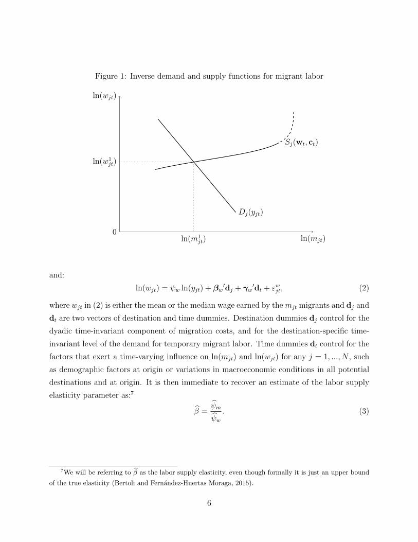
Figure 1: Inverse demand and supply functions for migrant labor

ln(mjt)

ln(wjt)

Dj(yjt)

Sj(wt, ct)

ln(w1jt)

ln(m1jt)

0

and:

ln(wjt) = ψw ln(yjt) + βw′dj + γw

′dt + εwjt, (2)

where wjt in (2) is either the mean or the median wage earned by the mjt migrants and dj and

dt are two vectors of destination and time dummies. Destination dummies dj control for the

dyadic time-invariant component of migration costs, and for the destination-specific time-

invariant level of the demand for temporary migrant labor. Time dummies dt control for the

factors that exert a time-varying influence on ln(mjt) and ln(wjt) for any j = 1, ..., N , such

as demographic factors at origin or variations in macroeconomic conditions in all potential

destinations and at origin. It is then immediate to recover an estimate of the labor supply

elasticity parameter as:7

β =ψm

ψw. (3)

7We will be referring to β as the labor supply elasticity, even though formally it is just an upper bound

of the true elasticity (Bertoli and Fernandez-Huertas Moraga, 2015).

6

2.3 Correlated variations in real GDP across destinations

The evolution of macroeconomic conditions across alternative destinations might be (posi-

tively or negatively) correlated; specifically, a pattern of predominantly positive correlations

entails that a rightward shift of the curve Dj(yjt) would be associated with a leftward shift

of the curve Sj(wt, ct), as potential migrants would face higher wages in alternative destina-

tions. This would produce an upward bias in the induced variation in migrants’ wages, and

a downward bias in the effect on the scale of migration flows to j, if the correlated shift in

the migrant labor supply is not controlled for, as depicted in Figure 2. This, in turn, would

imply that β would be downward biased.

Figure 2: Correlation between shifts in the inverse demand and supply functions

‘

ln(mjt)

ln(wjt)

Dj(y1jt) Dj(y

2jt)

Sj(w1t , ct)

Sj(w2t , ct)

ln(w1jt)

ln(w3jt)

ln(w2jt)

ln(m1jt)ln(m3

jt)ln(m2

jt)0

Note: the figure is drawn assuming a positive correlation in the evolution of real GDP across destinations.

However, this does not pose a serious threat to identification under the distributional

assumptions a la McFadden (1974), as these entail that the inverse supply curves for different

destinations are identical up to a constant. Hence, this confounding effect is fully controlled

for in the estimation of (1) and (2) through the inclusion of time dummies dt.8 This also

8This is, a fortiori, the case in the presence of binding minimum wages, as shifts in the labor supply are

7

applies under the distributional assumptions of Ortega and Peri (2013), which allow for

unobserved individual heterogeneity in the preferences for migration, as the function that

describes the influence of the attractiveness of alternative destinations on the migrant labor

supply is still invariant across destinations.

Correlated variations in macroeconomic conditions across destinations pose a more seri-

ous threat to identification under more general distributional assumptions, which allow for

differences in the elasticities of substitution across different pairs of destination countries

(Bertoli and Fernandez-Huertas Moraga, 2013, 2015), and that can be motivated by an in-

complete specification of the deterministic component of location-specific utility.9 Imagine,

for instance, that potential Filipino migrants perceive South Korea (j) and Malaysia (h) as

close substitutes, while the United States (k) represent a distant substitute for both desti-

nations: an increase in the attractiveness of Malaysia induces a proportional reduction in

the supply of Filipino migrants to South Korea at the contracted wage wjt that exceeds

the corresponding proportional reduction in the supply of Filipino migrants to the United

States at the contracted wage wkt. In other terms, the inverse supply functions Sj(wt, ct)

and Sk(wt, ct) do not follow an identical time profile over time, and the use of time dummies

dt no longer suffices to control for the shifts over time of the inverse supply functions.

If this threat is not adequately controlled for, then the error terms of (1) and (2) will be

serially correlated, as the attractiveness of alternative destinations is likely to evolve slowly

over time, and correlated across destinations if some destination countries have similar sets

of destinations that are perceived as close substitutes to each of them, e.g., Malaysia might

be a close substitute for both South Korea and Indonesia. The non-spherical nature of the

error term can produce inconsistently estimated standard errors, and, more importantly, it

gives rise to an endogeneity problem for ln(yjt) when the economic shocks in destination j

are correlated with the economic shocks in other destinations that are close substitutes to

j. This can create a serious threat to identification, as shifts in the labor demand curve

in destination j can be correlated with shifts in the labor supply due to changes in the

attractiveness of other destinations. Specifically, if there is a positive correlation in the

evolution of economic conditions in destinations that are regarded as close substitutes, then

a rightward shift in the labor demand curve is associated with a leftward shift in the supply

immaterial as long as the minimum wage remains binding.9This could occur, for instance, if the assumption that cjt = cj + ft for all j ∈ D is incorrect, as the

relative accessibility of different destinations varies over time.

8

curve, leading to a downward bias in the estimate of ψm and to an upward bias in the

estimate of ψw. This situation is depicted in Figure 2. The relative importance of the bias

on the two coefficients of interest depends on the elasticity of the labor demand schedule. If

the labor demand is flatter, and hence more elastic, then the correlation in macroeconomic

shocks across destinations will induce a larger bias in the estimate of ψm than of ψw.10 The

opposite pattern of correlation would reverse the direction of the bias in the estimation of

ψm and ψw.

2.4 Dealing with the threat to identification

Bertoli and Fernandez-Huertas Moraga (2013) demonstrate that the Common Correlated

Effects, CCE, estimator proposed by Pesaran (2006) allows us to control for the threat to

identification posed by the dependence of the migrant labor supply on the attractiveness of

alternative destinations.11 The CCE estimator calls for adding a set of auxiliary regressors

corresponding to destination-specific effects of the cross-sectional averages of the dependent

variable and of all the independent variables in the model. In the case of the reduced-form

migration regression, this amounts to estimating:

ln(mjt) = ψm ln(yjt) + βm′dj + φmj

′zt + εmjt, (4)

where:12

zt =1

N

(N∑j=1

ln(mjt),N∑j=1

ln(yjt)

)′.

Similarly, for the wage regression we can estimate:

ln(wjt) = ψw ln(yjt) + βw′dj + φwj

′zt + εwjt. (5)

We can observe that (4) reduces to (1) if we impose the restriction that φmj = φm for

any j,13 and that (5) reduces to (2) if φwj = φw. In this sense, the fixed effects models

10If the labor demand is infinitely elastic, i.e., φ = 0, then the presence of correlated shocks does not

induce a bias in the estimation of ψw.11Notice that the CCE estimator can accommodate serial correlation and cross-sectional dependence in

the error term (Pesaran and Tosetti, 2011).12If weights are used in the estimation, then auxiliary regressors are computed through weighted cross-

sectional averages.13With this restriction, we have that φm = (1,−ψm)′, as the inclusion of time dummies dt is equivalent to

9

in (1) and (2) are nested in the CCE estimator. Hence, we will refer to (4) and (5) as the

unrestricted specifications and to (1) and (2) as the restricted specifications. In terms of the

interpretation of the estimates, this is the difference between assuming that all destination

countries are equally substitutable for potential migrants, as in Ortega and Peri (2013), and

assuming different patterns of substitution across destinations for potential countries, as in

Bertoli and Fernandez-Huertas Moraga (2013, 2015). The more complicated error structure

would also affect the computation of the labor supply elasticity in equation (A.10). Still, it

would not change the interpretation of the parameter β = ψm/ψw as an upper bound on the

true elasticity.

3 Data and descriptive statistics

We use the bilateral data on the scale of temporary Filipino migration and on migrants’ wages

between 1992 and 2009 collected by the Philippines Overseas Employment Administration

(POEA).14 Our analysis draws on the replication files by McKenzie et al. (2014), which

include information on the (total and gender-specific) number of new hires and on the median

and mean hiring wages to 54 destination countries.15 New hires are defined as all the instances

in which land-based overseas Filipino workers sign a temporary contract with a new employer;

this definition thus includes both first-time migrants and migrants that change their job at

destination.16 The destination countries included in the sample recorded a positive number

of new hires in each year, and accounted for no less than 85 percent of the total number of

new hires of Filipino workers in the world for every year between 1992 and 2009.

Figure 3 plots the evolution of the total number of new hires and the mean of the nominal

wage reported in the contracts between 1992 and 2009 for our sample of destination countries.

The number of new hires increases, although not steadily so, over time, oscillating between

taking the difference of the dependent and of the independent variable(s) from the respective cross-sectional

averages.14Migrants’ average monthly wages wjt are measured in current US dollars.15We rely on the logarithm of the mean wage, as in Ottaviano and Peri (2012) and in McKenzie et

al. (2014), even though this choice is regarded “unconventional” by Borjas et al. (2012). The underlying

individual wages that we would need to compute the mean of the log wage are not publicly available. This

choice has the advantage of making our results directly comparable with those from McKenzie et al. (2014).16McKenzie et al. (2014) report that new hires represent 38 percent of all the contracts processed by the

POEA between 1998 and 2009, with rehires constituting the remainder.

10

Figure 3: Number of new hires and mean wage, 1992-2009

New hires

Thousands

Mean wage

USD19

92

1993

1994

1995

1996

1997

1998

1999

2000

2001

2002

2003

2004

2005

2006

2007

2008

2009

150

180

210

240

270

300

500

600

700

800

900

1,000

1,100

Note: total number of new hires (left axis) and mean wage (right axis) across the 54 destination countries

included in the analysis.

Source: Authors’ elaboration on the replication files from McKenzie et al. (2014).

193,453 new hires in 1996 and 290,545 in 2008. The mean wage increases from 600 USD in

1992 to 1,046 USD in 2009. Table 1 reports the number of total new hires over our period

of analysis for each of the 54 countries in our sample. Saudi Arabia represents the main

destination country, accounting for 30.02 percent of the total number of new hires over our

period of analysis, followed by Japan, Taiwan and the United Arab Emirates, with each of

these three countries representing more than 10 percent of the total number of new hires.17

17Japan introduced in 2005 new rules for the recruitment of temporary Filipino migrants, in response to

allegations about the exploitation of female Filipino migrants, who had been “almost exclusively employed

as overseas performing artists” (Theoharides, 2013, p. 26); these new rules led to a collapse in the number

of new hires, which went down from 71,636 in 2004 to 7,107 in 2007, and then further declined to 1,882 in

2009.

11

Table 1: New hires (1992-2009)

Destination Total Sharea Destination Total Sharea

Saudi Arabia 906,971 30.02 Cuba 2,303 0.08

Japan 471,467 15.60 New Zealand 2,199 0.07

Taiwan 419,551 13.89 China 2,173 0.07

United Arab Emirates 357,851 11.84 Yemen 1,445 0.05

Hong Kong 257,007 8.51 Indonesia 968 0.03

Kuwait 194,337 6.43 Micronesia 957 0.03

South Korea 48,023 1.59 India 796 0.03

Canada 41,158 1.36 Vietnam 781 0.03

Singapore 40,523 1.34 Pakistan 660 0.02

Bahrain 40,018 1.32 Thailand 594 0.02

Brunei Darussalam 28,197 0.93 Ghana 514 0.02

Israel 27,840 0.92 Norway 492 0.02

United Kindgom 25,649 0.85 Netherlands 490 0.02

United States 25,541 0.85 South Africa 480 0.02

Oman 20,077 0.66 Greece 417 0.01

Italy 16,392 0.54 Marshall Islands 412 0.01

Malaysia 15,275 0.51 Switzerland 298 0.01

Cyprus 13,526 0.45 Belgium 296 0.01

Spain 11,381 0.38 Finland 281 0.01

Jordan 10,802 0.36 Syria 215 0.01

Australia 7,910 0.26 Sri Lanka 207 0.01

Algeria 5,808 0.19 France 194 0.01

Russia 4,438 0.15 Fiji 181 0.01

Angola 4,333 0.14 Solomon Islands 163 0.01

Papua New Guinea 3,727 0.12 Austria 156 0.01

Sudan 3,416 0.11 Germany 132 0.00

Palau 2,415 0.08 Sweden 74 0.00

Notes: a share over the total number of new hires to the 54 destinations.

Source: Authors’ elaboration on the data from McKenzie et al. (2014).

The POEA also provides estimates of the stock of temporary Filipino workers and of

the total number of Filipinos residing in each destination in December 2009, at the end

of our period of analysis. The data reveal that temporary migration represents the main

–at times, nearly the unique– entry door for Filipino migrants in a number of destination

countries: for instance, 98.2 percent of Filipinos residing in Saudi Arabia in December 2009

were temporary migrants, and the median share of temporary migrants over our sample of

12

destination countries stands at 69.3 percent.18,19

The geographically diverse set of destination countries in our sample clearly experienced

a different evolution in their macroeconomic conditions over our period of analysis, but it is

important to observe that business cycle conditions of destination countries located in the

same region display a remarkable degree of (positive) correlation, which might pose a threat

to identification, as discussed in Section 2. For instance, Figure 4 plots the evolution of real

GDP growth between 1993 and 2009 for South Korea and Malaysia, to give a visual feeling

of the extent of the correlation in the evolution of macroeconomic conditions in relevant

destinations for Filipino migrants.

Figure 4: Real GDP growth rates for Malaysia and South Korea, 1993-2009

Growth rate

(percent)

1993

1994

1995

1996

1997

1998

1999

2000

2001

2002

2003

2004

2005

2006

2007

2008

2009

-5.0

0.0

5.0

10.0

Malaysia

South Korea

Source: Authors’ elaboration on World Bank (2015).

Overall, the average correlation of GDP growth across the 54 countries in the sample is

actually 0.24 but this goes up to 0.41 when we confine ourselves to the ten main destinations

18Authors’ elaboration on POEA, Stock estimates of Filipinos Overseas (Inter-Agency Report), available

at: http://www.poea.gov.ph/stats/statistics.html (last accessed on June, 25, 2015).19Other channels of entry, such as family reunification provisions, appear to dominate in some OECD

destinations–such as Canada, the United States or Australia, where temporary migrants only represent a

limited fraction of the total stock of Filipino immigrants.

13

(see Table 1), and even to 0.75 if we concentrate on the six East Asian countries, namely

Japan, Taiwan, Hong Kong, South Korea, Singapore and Malaysia, which account for more

than 40 percent of new hires.20 This implies that the concern about the threat to identifi-

cation posed by correlated variations in macroeconomic conditions across destinations has a

strong empirical relevance in this case.

4 Econometric analysis

We present here the results from the estimation of the restricted and unrestricted versions

of the wage and of the migration equations, and the ensuing values for the elasticity of the

migrant labor supply.21 All our results are robust when we rely on median rather than

mean wages as the dependent variable in the wage equation, and when we estimate the wage

equation separately on the sub-sample of male and female Filipino migrants; the Appendix

A.2 reports these additional specifications.22 23

4.1 Reduced form wage equation

Table 2 presents three different ways of estimating the relationship between mean wages of

overseas Filipino workers and contemporaneous GDP shocks.24 In Column (1), we present

the estimate of the restricted version of (5), i.e., we estimate (2), and we assign an equal

weight to each observation. The elasticity of the mean wage with respect to GDP per

capita is statistically zero in an unweighted estimation with destination and year fixed ef-

fects. However, things change drastically in Column (2), where we weight the observations

corresponding to each destination-year by the corresponding total number mjt of overseas

20Similarly, the average pairwise correlation of real GDP growth across the 15 European countries in

Table 1 stands at 0.73.21The restricted versions of the wage and of the migration equations assume that all destination countries

are equally substitutable for potential migrants, while the unrestricted versions allow for different patterns

of substitution across destinations for potential migrants (see Section 2.4).22We also present in the Appendix A.2 the regressions run on a sample that excludes Japan, given the

collapse in the number of (mostly female) new hires to this destination after 2005 that was induced by the

change in recruitment policies (Theoharides, 2015).23The estimates are also robust to the exclusion of the main destination (Saudi Arabia) from the sample;

results are available from the authors upon request.24Wage data are missing for 5 out of 972 observations.

14

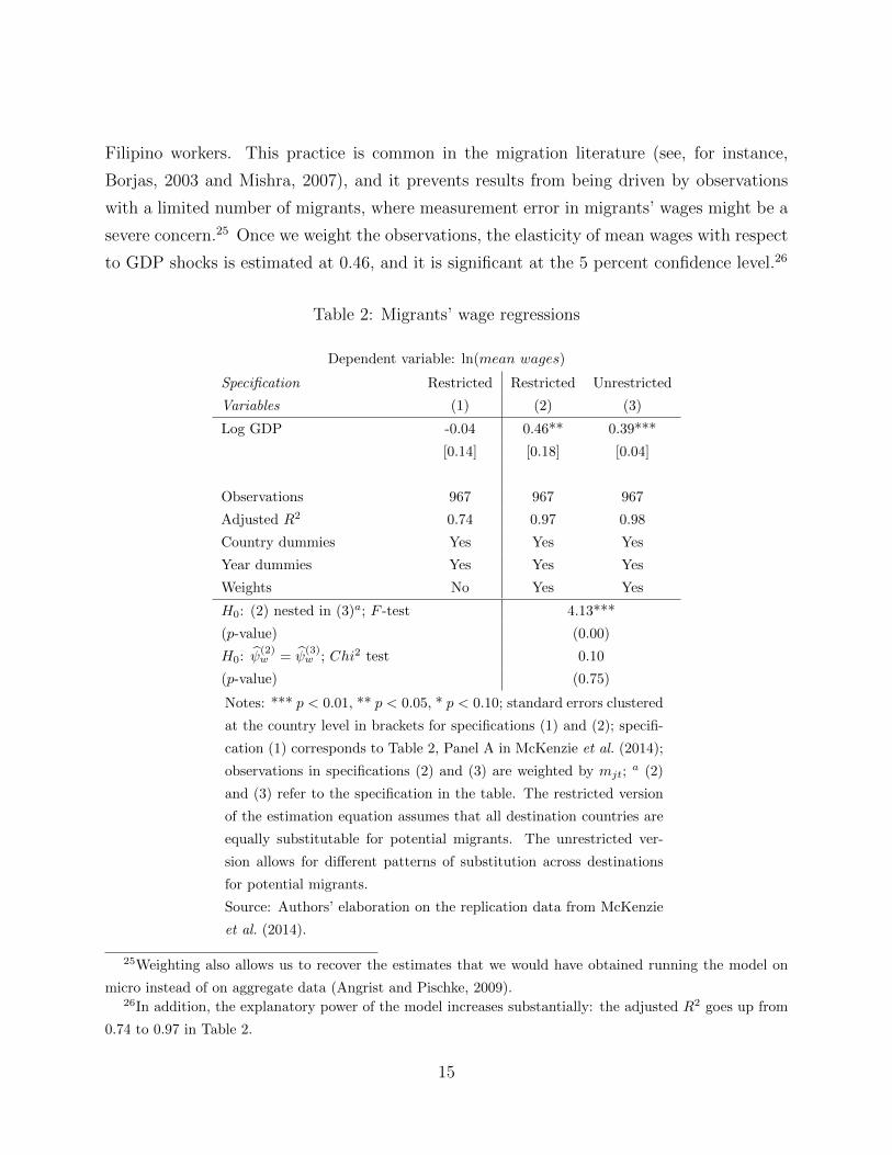
Filipino workers. This practice is common in the migration literature (see, for instance,

Borjas, 2003 and Mishra, 2007), and it prevents results from being driven by observations

with a limited number of migrants, where measurement error in migrants’ wages might be a

severe concern.25 Once we weight the observations, the elasticity of mean wages with respect

to GDP shocks is estimated at 0.46, and it is significant at the 5 percent confidence level.26

Table 2: Migrants’ wage regressions

Dependent variable: ln(mean wages)

Specification Restricted Restricted Unrestricted

Variables (1) (2) (3)

Log GDP -0.04 0.46** 0.39***

[0.14] [0.18] [0.04]

Observations 967 967 967

Adjusted R2 0.74 0.97 0.98

Country dummies Yes Yes Yes

Year dummies Yes Yes Yes

Weights No Yes Yes

H0: (2) nested in (3)a; F -test 4.13***

(p-value) (0.00)

H0: ψ(2)w = ψ

(3)w ; Chi2 test 0.10

(p-value) (0.75)

Notes: *** p < 0.01, ** p < 0.05, * p < 0.10; standard errors clustered

at the country level in brackets for specifications (1) and (2); specifi-

cation (1) corresponds to Table 2, Panel A in McKenzie et al. (2014);

observations in specifications (2) and (3) are weighted by mjt;a (2)

and (3) refer to the specification in the table. The restricted version

of the estimation equation assumes that all destination countries are

equally substitutable for potential migrants. The unrestricted ver-

sion allows for different patterns of substitution across destinations

for potential migrants.

Source: Authors’ elaboration on the replication data from McKenzie

et al. (2014).

25Weighting also allows us to recover the estimates that we would have obtained running the model on

micro instead of on aggregate data (Angrist and Pischke, 2009).26In addition, the explanatory power of the model increases substantially: the adjusted R2 goes up from

0.74 to 0.97 in Table 2.

15

Column (3) presents the results of estimating the unrestricted version of version of (5).

The F -test, which is conducted on the null hypothesis that φwj = φw, reveals that the

coefficients of the auxiliary regressors added by the CCE procedure vary across destinations,

thus validating the need to lift the restriction upon which the estimation of (2) reported in

Column (2) is based. The estimated elasticity in Column (3), which is significant at the 1

percent confidence level, is very similar in magnitude to the one observed in Column (2).

The elasticity decreases, as predicted by the theory in the empirically relevant scenario of

a predominantly positive correlation in macroeconomic conditions across destinations, but

only from 0.46 to 0.39, an insignificant difference at conventional levels. This result suggests

that labor demand is elastic enough so that substitutability patterns across destinations do

not affect migrant wages much.

4.2 Reduced form migration equation

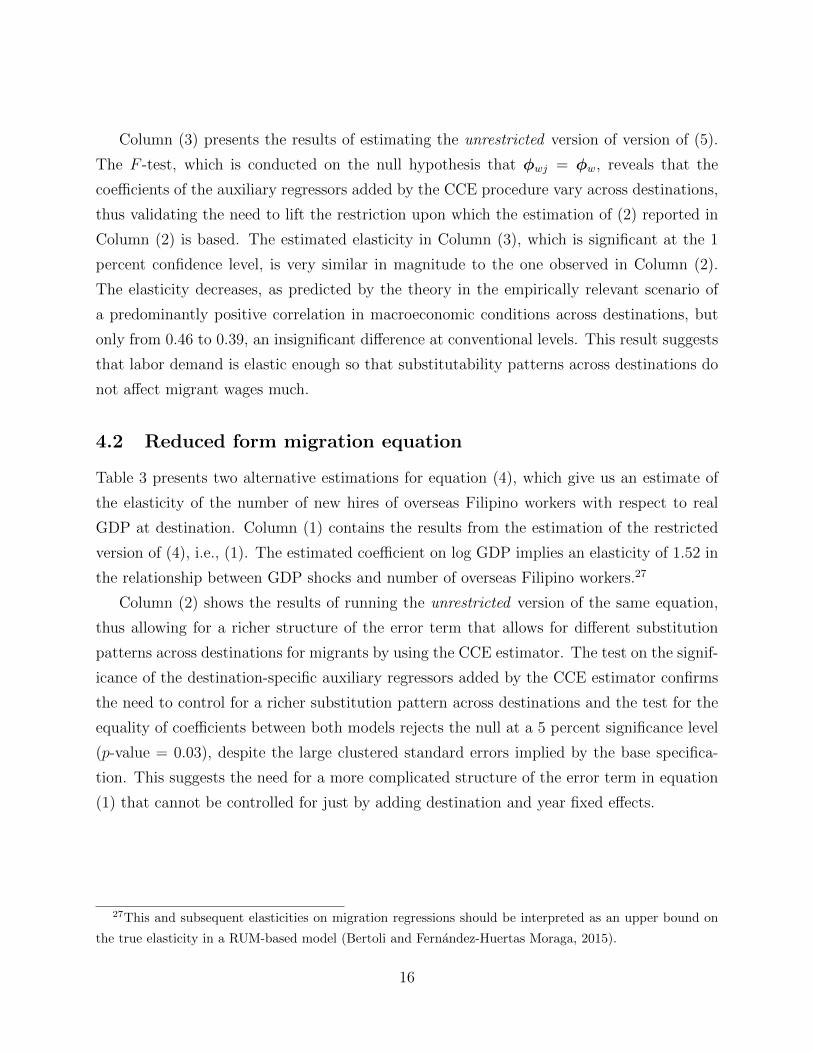
Table 3 presents two alternative estimations for equation (4), which give us an estimate of

the elasticity of the number of new hires of overseas Filipino workers with respect to real

GDP at destination. Column (1) contains the results from the estimation of the restricted

version of (4), i.e., (1). The estimated coefficient on log GDP implies an elasticity of 1.52 in

the relationship between GDP shocks and number of overseas Filipino workers.27

Column (2) shows the results of running the unrestricted version of the same equation,

thus allowing for a richer structure of the error term that allows for different substitution

patterns across destinations for migrants by using the CCE estimator. The test on the signif-

icance of the destination-specific auxiliary regressors added by the CCE estimator confirms

the need to control for a richer substitution pattern across destinations and the test for the

equality of coefficients between both models rejects the null at a 5 percent significance level

(p-value = 0.03), despite the large clustered standard errors implied by the base specifica-

tion. This suggests the need for a more complicated structure of the error term in equation

(1) that cannot be controlled for just by adding destination and year fixed effects.

27This and subsequent elasticities on migration regressions should be interpreted as an upper bound on

the true elasticity in a RUM-based model (Bertoli and Fernandez-Huertas Moraga, 2015).

16

Table 3: Migration regression

Dependent variable: ln(mjt)

Specification Restricted Unrestricted

Variables (1) (2)

Log GDP 1.52*** 3.38***

[0.50] [0.67]

Observations 972 972

Adjusted R2 0.85 0.90

Country dummies Yes Yes

Year dummies Yes Yes


(p-value) (0.00)

H0: ψ(1)m = ψ

(2)m ; Chi2 test 4.51**

(p-value) (0.03)

Notes: *** p < 0.01, ** p < 0.05, * p < 0.10; standard

errors clustered at the country level in brackets for specifi-

cation (1); specification (1) corresponds to Table 2, Panel

A in McKenzie et al. (2014); a (1) and (2) refer to the

specification in the table. The restricted version of the es-

timation equation assumes that all destination countries

are equally substitutable for potential migrants. The unre-

stricted version allows for different patterns of substitution

across destinations for potential migrants.

Source: Authors’ elaboration on the replication data from

McKenzie et al. (2014).

The estimated coefficient for GDP increases from 1.52 to 3.38. The elasticity estimated

in Column (1) is downward biased, as expected with a positive correlation in the evolution

of macroeconomic conditions across destinations (see Section 3), the case depicted in Figure

2. The intuition for the difference is straightforward. For each destination and year, the 1.52

coefficient was picking up both the direct positive effect of GDP shocks on migration to that

destination and that year and the indirect negative effect of correlated shocks in alternative

destinations or in the same destination in different years.

17

4.3 The implied elasticity of the migrant labor supply

The tests conducted on the estimates of the reduced form wage and migration equations

presented in Tables 2 and 3 reject the restrictions upon which equations (2) and (1) are

based. Thus, the unrestricted versions of the two reduced form equations–with weights

included in the wage equation–represent our preferred specifications. When we take the

ratio between ψm = 3.38 from Column (2) of Table 3 and ψw = 0.39 from Column (2) of

Table 2, we obtain an implied labor supply elasticity β of temporary Filipino migrants which

stands at 8.57 (s.e. = 2.91).28

As the estimation of the restricted versions of the two equations deliver a downward

biased estimate of ψm and an upward biased ψw, following the prediction of our simple

theoretical model, then they result in a significant underestimation of β, which stands at

3.34 (s.e. = 1.50). Dealing with the threats to identification in the reduced form regressions

proves to be crucial for a sound measurement of the elasticity of migrant labor supply.

5 Concluding remarks

The reaction of international migrants to wage differences across countries depends on the

interaction of the labor supply decisions of the workers and the labor demand situation in

every potential destination. This simple observation has implications on how we should

interpret the reduced form estimates from gravity models of international migration. In

particular, gravity equation parameters on economic conditions are not equivalent to labor

supply elasticities.

In this paper, we explicitly show the relationship between the estimates from a gravity

model of migration and the labor supply elasticity. We then go on to provide an example

by estimating an upper bound on the elasticity of the labor supply of temporary Filipino

migrant workers between 1992 and 2009. We find that the labor supply elasticity of this

subset of workers is as high as 8.57, which implies that temporary Filipino migrants are very

responsive to wages offered by employers at different destinations. Summing up, they retain

a very high ability to choose among competing offers by changing their destination.

From the point of view of host countries, this high responsiveness means that labor-

importing countries should not take temporary workers for granted. They will not be willing

28Bootstrapped standard errors from resampling 100 times with replacement.

18

to come if conditions become too harsh. A different issue, for future research, is the ability

of host countries to substitute unwilling Filipino workers with workers from other origins.

It would be interesting to understand whether the high labor supply elasticity of Filipino

migrants is matched by other countries of origin for temporary workers.

References

Angrist, J. D. and J.-S. Pischke (2009): Mostly Harmless Econometrics: An Empiri-

cist’s Companion, Princeton: Princeton University Press.

Bai, J. (2009): “Panel data models with interactive fixed effects,” Econometrica, 77, 1229–

1279.

Beine, M., S. Bertoli, and J. Fernandez-Huertas Moraga (2016): “A practitioners’

guide to gravity models of international migration,” The World Economy, 39, 596–612.

Bertoli, S., and J. Fernandez-Huertas Moraga (2013): “Multilateral Resistance to

Migration,” Journal of Development Economics, 102, 79–100.

Bertoli, S., and J. Fernandez-Huertas Moraga (2015): “The size of the cliff at the

border,” Regional Science and Urban Economics, 51, 1–6.

Borjas, G. J. (2003): “The Labor Demand Curve Is Downward Sloping: Reexamining

the Impact of Immigration on the Labor Market,” Quarterly Journal of Economics, 118,

1335–1374.

Borjas, G. J., J. Grogger and G. H. Hanson (2012): “Comment: on Estimating

Elasticities of Substitution,” Journal of the European Economic Association, 10(1), 198–

223.

Chetty, R., A. Guren, D. S. Manoli and A. Weber (2015): “Does Indivisible Labor

Explain the Difference between Micro and Macro Elasticities? A Meta-Analysis of Ex-

tensive Margin Elasticities,” Macroeconomics Annual 2012, University of Chicago Press,

27(1), 1–56.

Cortes, P. (2015): “The Feminization of International Migration and its Effects on the

Children Left Behind: Evidence from the Philippines,” World Development, 65, 62–78.

19

Driscoll, J. C., and A. C. Kraay (1998): “Consistent Covariance Matrix Estimation

with Spatially Dependent Panel Data,” Review of Economics and Statistics, 80, 549–560.

Kleven, H. J, C. Landais, E. Saez and E. Schultz (2014): “Migration and Wage

Effects of Taxing Top Earners: Evidence from the Foreigners’ Tax Scheme in Denmark,”

Quarterly Journal of Economics, 129(1), 333–378.

Licuanan, V., T. Omar Mahmoud, and A. Steinmayr (2015): “The Drivers of Di-

aspora Donations for Development: Evidence from the Philippines,” World Development,

65, 94–109.

MaCurdy, T., D. Green, and H. Paarsch (1990): “Assessing Empirical Approaches

for Analyzing Taxes and Labor Supply,” Journal of Human Resources, 25, 415–490.

McFadden, D. (1974): “Conditional logit analysis of qualitative choice behavior,” in Fron-

tiers in Econometrics, ed. by P. Zarembka, pp. 105–142. New York: Academic Press.

McKenzie, D., C. Theoharides, and D. Yang (2014): “Distortions in the International

Migrant Labor Market: Evidence from Filipino Migration and Wage Responses to Des-

tination Country Economic Shocks,” American Economic Journal: Applied Economics,

6(2), 49–75.

Milanovic, B. (2005): Global and International Inequality 1950–2000, Princeton: Prince-

ton University Press.

Milanovic, B. (2015): “Global Inequality of Opportunity: How Much of Our Income Is

Determined by Where We Live?,” Review of Economics and Statistics, 97, 452–460.

Mishra, P. (2007): “Emigration and wages in source countries: Evidence from Mexico,”

Journal of Development Economics, 82(1), 180–199.

Ortega, F., and G. Peri (2013): “The Role of Income and Immigration Policies in

Attracting International Migrants,” Migration Studies, 1(1), 47–74.

Ottaviano, G. I. P., and G. Peri (2012): “Rethinking the Effect of Immigration of

Wages,” Journal of the European Economic Association, 10(1), 152–197.

20

Pesaran, M. H. (2006): “Estimation and Inference in Large Heterogeneous Panels with a

Multifactor Error Structure,” Econometrica, 74, 967–1012.

Pesaran, M. H. and E. Tosetti (2011): “Large Panels with Common Factors and Spatial

Correlation,” Journal of Econometrics, 161(2), 182–202.

Pritchett, L. (2006): Let Their People Come. Washington: Center for Global Develop-

ment.

Rider, P. R. (1960): “Variance of the Median of Small Samples from Several Special

Populations,” Journal of the American Statistical Association, 55(289), 148–150.

Small, K. A., and H. S. Rosen (1981): “Applied Welfare Economics with Discrete Choice

Models,” Econometrica, 49(1), 105–130.

Theoharides, C. (2013): “Manila to Malaysia, Quezon to Qatar: International Migration

and the Effects of Origin-Country Human Capital,” mimeo, Ann Arbor: University of

Michigan.

Theoharides, C. (2015): “Banned from the Band: The Effect of Migration Barriers on

Origin-Country Labor Market Decisions,” paper presented at the Eight Migration and

Development Conference, June 2015, Washington.

World Bank (2015): World Development Indicators, Washington: The World Bank.

Yang, D. (2006): “ Why Do Migrants Return to Poor Countries? Evidence from Philippine

Migrants’ Responses to Exchange Rate Shocks,” Review of Economics and Statistics, 88,

715–735.

Yang, D. (2008): “International Migration, Remittances and Household Investment: Evi-

dence from Philippine Migrants’ Exchange Rate Shocks,” Economic Journal, 118, 591–630.

21

A Appendix

This appendix provides details on the model and the estimation equations discussed in the

paper, as well as supplemental tables referenced in the main text.

A.1 The market for temporary migrant labor

Let mjt represent the number of migrants that move on a temporary basis from an ori-

gin country to the destination country j = 1, ..., N at time t = 1, ..., T , and let wt =

(w0t, w1t, ..., wNt)′ and ct = (c0t, c1t, ..., cNt)

′ be two vectors that gather migrants’ wages and

bilateral migration costs and time t.29 The inverse demand function for temporary migrant

labor is given by:

wjt = ajyαjtm

−φjt , (A.1)

where yjt is the real GDP in country j at time t, and aj is a time-invariant parameter

that shifts the inverse labor demand in destination j. The supply of migrant labor can

be derived from an underlying static random utility maximization model that describes

the location-decision problem that potential migrants face, which represents the standard

micro-foundation of a gravity equation for migration (Beine et al., 2016). Specifically, if

the deterministic component of utility Vjt depends on the logarithm of the wage wjt and on

bilateral migration costs cjt, i.e., Vjt = β ln(wjt) − cjt, then the distributional assumptions

in McFadden (1974) on the individual-specific stochastic component εijt allow to write the

expected value of the labor supply mjt as follows:30

E(mjt) = wβjte−cjt−Ω(wt,ct)nt, (A.2)

where nt is the size of the population at origin, and:

Ω(wt, ct) = ln

(N∑k=0

wβkte−ckt

)

represents the expected value from the choice situation that potential migrants face at time

t (Small and Rosen, 1981). The function Ω(wt, ct) in (A.2), which describes the influence

29We let w0t denote the wage in the origin country at time t, and we normalize the cost of staying c0t to

zero.30We thus assume that εijt follows an independent and identically distributed Extreme Value Type-1

distribution.

22

exerted by the attractiveness of all countries on the expected value of the migrant labor

supply to destination j at time t, varies over time but it is invariant across destinations.

A.1.1 The elasticity of the labor supply

We can recover the elasticity of the migrant labor supply from (A.2) assuming, by the law

of large numbers, that E(mjt) = mjt. We have that:

∂ ln(mjt)

∂ ln(wjt)= β(1− pjt). (A.3)

The elasticity in (A.3) depends on the actual migration rate pjt ≡ mjt/nt between the origin

and each destination at time t. In practice, pjt will be very small for any j = 1, ..., N and

any t = 1, ..., T since only a tiny fraction of the Filipino population migrates to a single

destination in a given year, so that β(1− pjt) ≈ β, and we will be referring to β as the labor

supply elasticity, even though formally it is just an upper bound of the true elasticity.

We can rearrange the terms in (A.1) and (A.2) to obtain (a logarithmic transformation of)

the inverse demand function Dj(yjt) and the inverse supply function Sj(wt, ct) for migrant

labor in destination j, as:

D(yjt) = ln(aj) + α ln(yjt)− φ ln(mjt), (A.4)

and:

Sj(wt, ct) = β−1 [ln(mjt) + cjt + Ω(wt, ct)− ln(nt)] , (A.5)

We can observe from (A.5) that Sk(wt, ct) = Sj(wt, ct)+β−1(ckt−cjt), i.e., the inverse supply

functions for two destinations differ only by a term which is proportional to the difference

in the bilateral migration costs.

A.1.2 Reduced form regressions

We can derive the following reduced-form regression that gives us the elasticity of the scale

of migration with respect to the real GDP at destination combining (A.1) and (A.2) with

E(mjt) = mjt:

ln(mjt) =αβ

1 + φβln(yjt)−

1

1 + φβ[Ω(wt, ct) + cjt − ln(nt)] +

β

1 + φβln(aj) + εmjt . (A.6)

23

Similarly, the reduced-form regression that gives us the elasticity of migrants’ wages with

respect to the real GDP at destination can be written as:

ln(wjt) =α

1 + φβln(yjt) +

φ

1 + φβ[Ω(wt, ct) + cjt − ln(nt)] +

1

1 + φβln(aj) + εwjt. (A.7)

Under the assumption that the bilateral migration costs can have different levels across

destinations but follow an identical time profile,31 then the two elasticities of interest can be

identified through the estimation of the following two equations:

ln(mjt) = ψm ln(yjt) + βm′dj + γm

′dt + εmjt , (A.8)

and:

ln(wjt) = ψw ln(yjt) + βw′dj + γw

′dt + εwjt, (A.9)

where wjt in (A.9) is either the mean or the median wage earned by the mjt migrants and dj

and dt are two vectors of destination and time dummies. Destination dummies dj control

for the dyadic time-invariant component cj of migration costs, and for the term ln(aj) in

(A.4) that influences the level of the demand for temporary migrant labor. Time dummies

dt control for the factors that exert a time-varying influence on ln(mjt) and ln(wjt) for any

j = 1, ..., N , such as demographic factors at origin or variations in macroeconomic conditions

in all potential destinations and at origin.

It is then immediate from (A.6)-(A.9) to recover an estimate of the labor supply elasticity

parameter β in (A.3) as:

β =ψm

ψw. (A.10)

31Formally, we assume that cjt = cj +ft for all j ∈ D; this assumption implies that the difference between

Sk(wt, ct) and Sj(wt, ct), with j, k ∈ D, is time-invariant.

24

A.2 Additional specifications

Table A.1: Median wages

Dependent variable:

ln(median wages)



Log GDP -0.06 0.61** 0.78***

[0.16] [0.23] [0.05]


Adjusted R2 0.72 0.96 0.98



Weights No Yes Yes


(p-value) (0.00)

Test, H0: ψ(2)w = ψ

(3)w ; Chi2 test 0.49

(p-value) (0.48)

Notes: *** p < 0.01, ** p < 0.05, * p < 0.10; standard errors clustered at

the country level in brackets for specifications (1) and (2); specification (1)

corresponds to Table 2, Panel A in McKenzie et al. (2014); observations

in specifications (2) and (3) are weighted by mjt;a (2) and (3) refer to the

specification in the table. The restricted version of the estimation equa-

tion assumes that all destination countries are equally substitutable for

potential migrants. The unrestricted version allows for different patterns

of substitution across destinations for potential migrants.

Source: Authors’ elaboration on the replication data from McKenzie et

al. (2014).

25

Table A.2: Mean wages by gender

Dependent variable:

ln(mean wages)



Panel A: Male sample

Log GDP -0.03 0.46*** 0.33***

[0.12] [0.13] [0.09]


(p-value) (0.00)

H0: ψ(2)m = ψ

(3)m ; Chi2 test 0.64

(p-value) (0.42)


Adjusted R2 0.67 0.92 0.96

Panel B: Female sample

Log GDP 0.04 0.46*** 0.34***

[0.21] [0.16] [0.05]


(p-value) (0.00)

H0: ψ(2)w = ψ

(3)w ; Chi2 test 0.46

(p-value) (0.50)


Adjusted R2 0.75 0.98 0.98



Weights No Yes Yes



corresponds to Table 2, Panel B and C in McKenzie et al. (2014); observations

in specifications (2) and (3) are weighted by the gender-specific number of mi-

grants mjt;a (2) and (3) refer to the specification in the table. The restricted

version of the estimation equation assumes that all destination countries are

equally substitutable for potential migrants. The unrestricted version allows

for different patterns of substitution across destinations for potential migrants.

Source: Authors’ elaboration on the replication data from McKenzie et al.

(2014). 26

Table A.3: Median wages by gender

Dependent variable:

ln(median wages)




Log GDP -0.02 0.45** 0.19*

[0.15] [0.18] [0.10]


(p-value) (0.00)

H0: ψ(2)m = ψ

(3)m ; Chi2 test 1.66

(p-value) (0.20)


Adjusted R2 0.65 0.89 0.95


Log GDP -0.05 0.51*** 0.35***

[0.23] [0.18] [0.06]


(p-value) (0.00)

H0: ψ(2)w = ψ

(3)w ; Chi2 test 0.58

(p-value) (0.45)


Adjusted R2 0.74 0.97 0.98



Weights No Yes Yes



corresponds to Table 2, Panel B and C in McKenzie et al. (2014); observations

in specifications (2) and (3) are weighted by the gender-specific number of mi-

grants mjt;a (2) and (3) refer to the specification in the table. The restricted

version of the estimation equation assumes that all destination countries are

equally substitutable for potential migrants. The unrestricted version allows

for different patterns of substitution across destinations for potential migrants.


(2014). 27

Table A.4: Migration regression by gender

Dependent variable:

ln(mjt)


Variables (1) (2)


Log GDP 1.15** 3.61***

[0.53] [0.69]

H0: Col. (1) nested in (2)a; F -test 5.72***

(p-value) (0.00)

H0: ψ(1)m = ψ

(2)m ; Chi2 test 7.14***

(p-value) (0.01)




Log GDP 1.98*** 1.37**

[0.62] [0.63]


(p-value) (0.00)

H0: ψ(1)m = ψ

(2)m ; Chi2 test 0.62

(p-value) (0.43)





Notes: *** p < 0.01, ** p < 0.05, * p < 0.10; standard errors clus-

tered at the country level in brackets for specification (1); specifica-

tion (1) corresponds to Table 2, Panel A in McKenzie et al. (2014); a

(1) and (2) refer to the specification in the table. The restricted ver-

sion of the estimation equation assumes that all destination countries

are equally substitutable for potential migrants. The unrestricted

version allows for different patterns of substitution across destina-

tions for potential migrants.

Source: Authors’ elaboration on the replication data from McKenzie

et al. (2014).

28

Table A.5: Mean wages, omitting Japan

Dependent variable:

ln(mean wages)



log GDP -0.07 0.58*** 0.50***

[0.14] [0.15] [0.07]


Adjusted R2 0.73 0.90 0.94



Weights No Yes Yes


(p-value) (0.00)

H0: ψ(2)w = ψ

(3)w ; Chi2 test 0.19

(p-value) (0.67)


the country level in brackets for specifications (1) and (2); observations in

specifications (2) and (3) are weighted by mjt;a (2) and (3) refer to the

specification in the table. The restricted version of the estimation equation

assumes that all destination countries are equally substitutable for potential

migrants. The unrestricted version allows for different patterns of substitu-

tion across destinations for potential migrants.


(2014).

29

Table A.6: Median wages, omitting Japan

Dependent variable:

ln(median wages)



log GDP -0.09 0.79*** 0.68***

[0.16] [0.18] [0.08]


Adjusted R2 0.70 0.89 0.94



Weights No Yes Yes


(p-value) (0.00)

H0: ψ(2)w = ψ

(3)w ; Chi2 test 0.25

(p-value) (0.62)


the country level in brackets for specifications (1) and (2); observations in

specifications (2) and (3) are weighted by mjt;a (2) and (3) refer to the

specification in the table. The restricted version of the estimation equation

assumes that all destination countries are equally substitutable for potential

migrants. The unrestricted version allows for different patterns of substitu-

tion across destinations for potential migrants.


(2014).

30

Table A.7: Migration regression omitting Japan

Dependent variable

ln(mjt)


Variables (1) (2)

log GDP 1.34*** 3.45***

[0.47] [0.67]






(p-value) (0.00)

H0: ψ(1)m = ψ

(2)m ; Chi2 test 5.97**

(p-value) (0.02)

Notes: *** p < 0.01, ** p < 0.05, * p < 0.10; standard errors

clustered at the country level in brackets for specification (1); a

(1) and (2) refer to the specification in the table. The restricted

version of the estimation equation assumes that all destination

countries are equally substitutable for potential migrants. The

unrestricted version allows for different patterns of substitution

across destinations for potential migrants.

Source: Authors’ elaboration on the replication data from

McKenzie et al. (2014).

31

the elasticity of the migrant labor supply: evidence from ...ftp.iza.org/dp10031.pdf · the...

Documents