MASSACHUSETTS INSTITUTE OF TECHNOLOGYARTIFICIAL INTELLIGENCE LABORATORY

A. I. Working Paper No. 262 August, 1984

The EIGHT Manual:A System for Geometric Modellingand Three-Dimensional Graphics

on the Lisp Machine

Bruce R. Donald

Abstract. We describe a simple geometric modelling system called Eight whichsupports interactive creation, editing, and display of three-dimensional polyhedralsolids. Perspective views of a polyhedral environment may be generated, andhidden surfaces removed. Eight proved useful for creating world models, and asan underlying system for modelling object interactions in robotics research andapplications. It is documented here in order to make the facility available to othermembers of the Artificial Intelligence Laboratory.

A.I. Laboratory Working Papers are produced for internal circulation, andmay contain information that is, for example, too preliminary or too detailed forformal publication. It is riot intended that they should be considered papers towhich reference can be made in the literature.@ Massactusctts Institute of Technology, 1984.

Acknowledgements. Philippe Brou wrote the Dover program, which maybe used to send the graphics produced by Eight to the Dover printer. John Cannyhelped write part of the polyhedral intersection facility. This manual was written,and Eight was revised, while the author was sponsored research staff at the A.I.Lab.

1

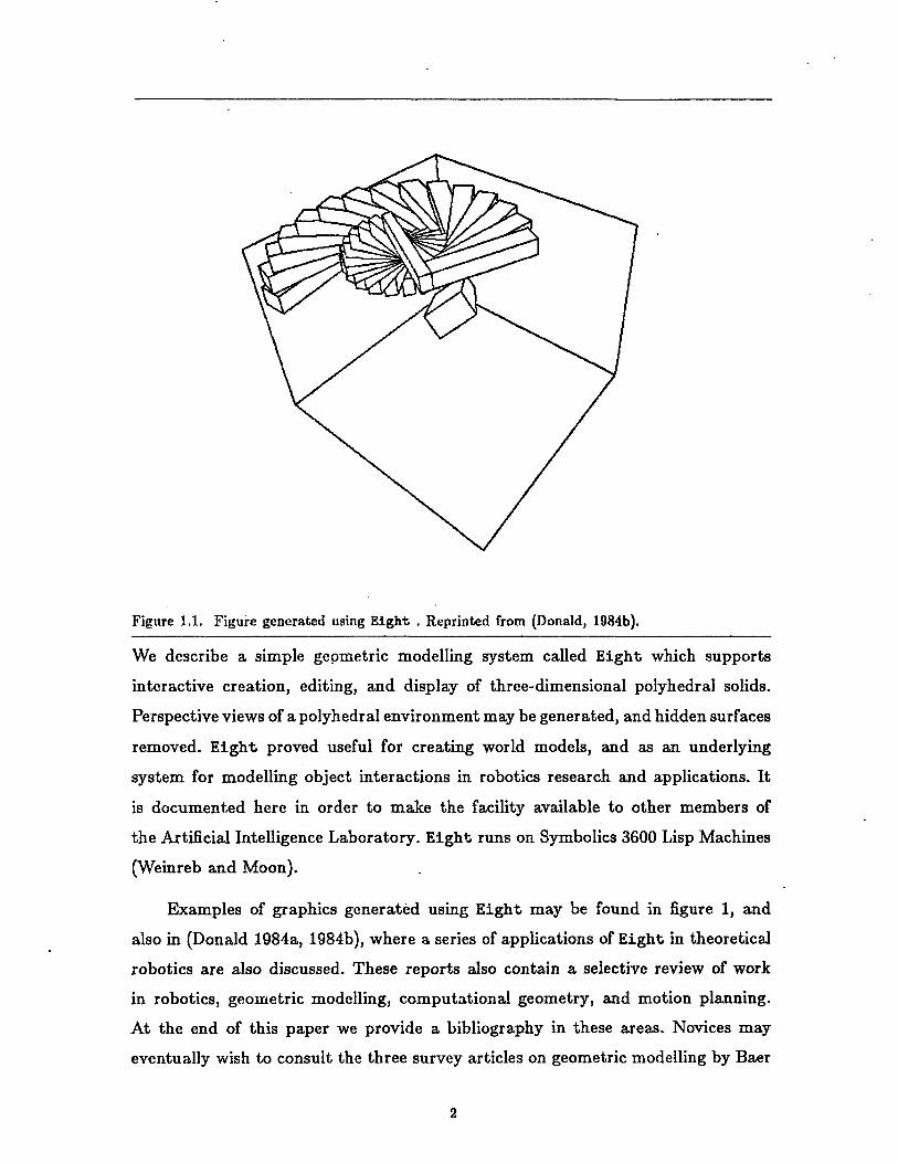
Figure 1.1. Figure generated using Eight . Reprinted from (Donald, 1984b).

We describe a simple geometric modelling system called Eight which supports

interactive creation, editing, and display of three-dimensional polyhedral solids.

Perspective views of a polyhedral environment may be generated, and hidden surfaces

removed. Eight proved useful for creating world models, and as an underlying

system for modelling object interactions in robotics research and applications. It

is documented here in order to make the facility available to other members of

the Artificial Intelligence Laboratory. Eight runs on Symbolics 3600 Lisp Machines

(Weinreb and Moon).

Examples of graphics generated using Eight may be found in figure 1, and

also in (Donald 1984a, 1984b), where a series of applications of Eight in theoretical

robotics are also discussed. These reports also contain a selective review of work

in robotics, geometric modelling, computational geometry, and motion planning.

At the end of this paper we provide a bibliography in these areas. Novices may

eventually wish to consult the three survey articles on geometric modelling by Baer

et al., Requicha, and Sutherland et al., and perhaps the book by Foley and van

Dam. Basic knowledge of Lisp Machine operation and Zetalisp is assumed.

Eight stands both for Eight Is a Graphics Hack, Too, and also for Eight Is

a Geometry Hack, Too.

1. Introduction: Basic Features

We begin with a hands-on tutorial to introduce the interactive graphic facilities

of Eight . Eight is loaded by typing (load "oz:ps:<brd>Eight .lisp"). Answer

"Y(es)" to the questions that ask whether you want to load up the 3-D (three

dimensional) system.

Now, Eight works by allowing you to create objects and enter them into

an environment. Once an environment is created, you can draw the, objects in it

(and also perform other operations on them). However, when Eight is loaded, the

environment is empty. We will construct objects and add them to the environment

later; for now, type (load " oz:ps: <brd>sample-environment .lisp"). For now,

all you need to know is that an environment is a collection of 0 or more polyhedra,

and that each polyhedron is represented in the environment by a geometric model

containing its faces, edges, and vertices, and their inter-relations.

Now that an environment is loaded, you must give commands to draw it.

You can either call Lisp functions explicitly or call up an interactive menu. Let

us explore the menu now: invoke it with <Function>-D. A wire-frame scene will

appear, with a menu below it.

The equivalent Lisp function for calling up the menu is:

channels:choose

Invokes the graphics command window.

1.1. Changing the Perspective

To change the perspective view, click on Left, Right, Up, or Down on the menu.

The perspective view is specified via a station-point (where you are standing), a

center of vision point (where you are looking), and a focal ratio (which specifies

what kind of camera you are using). Left, Right, Up, and Down all move the

station-point, keeping the center of vision and focal ratio fixed. To change the focal

ratio, click on Zoom in or Zoom out.

Now, these parameters correspond to variables in the Lisp world. You can

change them directly by clicking on Set Viewing Parameters. Alternatively, you

can bind them yourself:

channels:*eye Variable

A list of three real numbers representing the station point.

channels:*view Variable

A list of three real numbers representing the center of vision point.

channels:*focal Variable

A real number representing the focal ratio. The focal ratio is a parameter

in the perspective transformation rougly analogous to the "zoom factor" in

camera lenses.

When you set these parameters using the menu, Eight automatically recomputes

the perspective transformation for you, before drawing the environment. However,

if you bind them yourself, you must initiate this recomputation yourself by calling

the function channels:mapini:

channels:mapini

Initialize the perspective transformation with the current values of chan-

nels:*eye, channels:*view, and channels:*f ocal. (The perspective trans-

formation is a map from real-space coordinates to perspective coordinates,

which should explain the name mapini).

By default, Eight generates wire-frame views of the environment. All the edges

of all the polyhedra are drawn. Thus hidden surfaces, which would be obstructed

in real views, are not removed. To generate a view with hidden surfaces removed,

click on Hide.

1.2. Getting at Things in the Environment

Now, suppose you wanted to draw an environment from inside an applications

package. You know how to set up the viewing parameters. However, you also need

to know how to get at objects in the environment, and how to pass them to the

graphics routines.

Each polyhedron is a structure of type solid, and can be thought of as a

directed graph of structures which are faces, edges, and vertices (collections of

vertex structures). The precise organization of these objects is discussed later.

An environment is a flavor instance containing collections of solids, faces, and

edges. Eight only deals with one environment at a time; the current environment

is available via the macro

new:current-environment Macro

Returns the current environment.

* Henceforth, all Lisp forms are assumed to be in package new:, unless otherwise

indicated.

Thus it is possible to create one environment called *robot-environment*

containing a geometric model of a robot arm, another environment called

*obstacle-environment* containing geometric models of the obstacles, and

*workspace-boundary* containing the bounding walls around the workspace. To

draw or manipulate a different environment, you use the special form in-model-

environment to bind the current environment to the environment you wish to

manipulate:

in-model-environment environment-instance body... Macro

environment-instance must be an instance of flavor environment. Executes

the forms in body with the current environment bound to environment-

instance.

Now, the two main drawing functions are draw-edges, which draws a wire-

frame perspective view of a list of edges, and hide, which generates a hidden-surface

perspective view given a list of faces.

disflush

Clears the graphics screen.

draw-edges list-of-edges

Draw a wire-frame perspective view of the list of edges.

hide &optional (list-of-faces (get-faces)) (clear-screen-p T)

Generate a hidden-surface perspective view of the faces specified by list-of-

faces. Clear the screen first if clear-screen-p is T. The list of faces defaults

to the faces in the current environment.

Hide invokes an implementation of Newell's hidden-surface algorithm.' For

the hidden-surface view to be correct, the faces passed to hide should bound

non-intersecting polyhedra. Hide will not perform correctly if there is cyclic

overlap from the currect viewpoint. Cyclic overlap occurs when face ft obscures

a portion of face f2, f2 obscures a portion of f3, ... , fi-1 obscures fi, and

fi obscures fl. These cycles can be arbitrarily long. In case of cyclic overlap,

the view generated may be incorrect. A diagnostic message is displayed. By

changing the perspective slightly, you can usually eliminate cyclic overlap.

*cyclic- overlap- action* Variable

Determines what happens when cyclic overlap is detected. If this variable is

:warn, a warning is displayed. :beep beeps but prints no warning. :none

inhibits any warning. :flame displays a diagnostic message, and offers to show

you the cycle of faces. In all cases, Eight attempts to generate a view as best

it can. :flame is the default.

The following functions look at an environment and return a list containing all

the solids, faces, edges, or vertices in that environment. The environment argument

defaults to the current environment. The list get-faces is worthy of being passed

'Sce (Sutherland, et al.) for a tutorial.

to hide; similarly, the list of edges returned by get-edges may be passed to

draw-edges.

get-solids &optional (environment (current-environment))

Return a list of solids that are in environment.

get-faces &optional (environment (current-environment))

Return a list of faces that are in environment.

get-edges &optional (environment (current-environment))

Return a list of edges that are in environment.

get-vertices &optional (environment (current-environment))

Return a list of vertices that are in environment.

Example: Suppose we want a function to draw a hidden-surface perspective

view of the robot amidst the obstacles. Recall that the geometric models for the

robot and the obstacles are in two different environments. The following function

will do the trick, by merging the face lists from both environments.

(defun draw-peril ()(hide (append

(get-faces *robot-environment*)(get-faces *obstacle-environment*))))

1.3. Creating Polyhedra: Extrusion and Digitizing

The easiest way to create polyhedra is to click on Digitize on the Eight

command menu. This option allows you to digitize a polyhedron, that is, to input

its coordinates from the mouse. The polyhedron you digitize is added to the current

environment.

Suppose, however, you want to add the new polyhedron to the *obstacle-

environment*, instead of the current-environment. This may be accomplished as

follows:

(in-model-environment *obstacle-environment*(channels:choose))

channels:choose puts up the Eight command menu, and any new polyhedra

you digitize are added to the current environment, which happens to be bound to

*obstacle-environment*.

Incidentally, suppose you wanted to create a new environment, call *another-

obstacle-environment* to test your program. For example, the new environment

might contain a obstacle course for a path planner. If the current environment was

empty you could call channels:choose to digitize your environment, and then

say (setq *another-obstacle-environment* (current-environment)). This

has the disadvantage, however, that any subsequent modification of the current

environment will also affect *another-obstacle-environment*. The macro in-

new-environment is designed to solve this problem.

in-new-environment forms Macro

Create a new environment, and execute forms within it. Upon exit, restore the

current environment. Return the value of the last form in forms. Note that

the new environment will be lost (it is "popped" at the end) unless we retain

a pointer to it as follows:

Example:

(setq *another-obstacle-environment*(in-new-environment

(channels : choose)(current-environment)))

In this example, any solids we digitize in the Eight menu invoked by chan-

nels:choose, will be entered into the new environment. The new environment is

returned, and *another-obstacle-environment* is bound to it.

1.3.1. Extrusion

When you click on Digitize, a digitizing menu pops up which lets you choose

digitizing options. You can digitize a class of polyhedra called generalized prisms,

which can be created through a process called extrusion. A generalized prism P is

a polyhedron that can be represented by the vector sum of a polygon A embedded

in some plane Q in 3-space, and a three-dimensional sweep vector v orthogonal2 to

Q. Thus

P = A Ev,

where A v = {p + v Ip E A}. Thus to create P, we sweep a polygon A

over a vector v, and the resulting swept volume is P. Thus process is also called

extrusion, and A is sometimes termed a die polygon. For example, to create a cube

100 X 100 X 100, we could sweep the polygon

A == { (0, 0, 0), (0, 100, 0), (100, 100, 0), (100, 0, 0) }

over the vector v = (0, 0, 100).

It should be clear that in order to create generalized prisms, we need to specify:

(i) The plane Q on which A lies. Q is called the digitizing plane.

(ii) The coordinates of A on the plane. A is called the die polygon.

(iii) The 3-dimensional vector v. v is called the sweep vector.

The Digitize option allows the following choices. The digitizing plane Q may

be any of the x-y, y-z, or x-z planes. The sweep vector v is specified by two

parameters, the base slice and the top slice of the plane. Thus the cube above would

have selected the x-y plane as the digitizing plane, with a base slice of 0 and a

top slice of 100. In short, since we know the sweep vector must be parallel to the

excluded axis, it can be specified by its extent alone.

The coordinates of the die polygon A are digitized with the mouse, relative to

the selected plane. You click left for each new point in the coordinate loop, and

click right for the last point in the loop. Eight closes the loop for you. Middle

aborts.

Incidentally, to make vectors, such as v, employ the constructor macro:

make-vector &rest coordinates Macro

Construct and return a vector made out of coordinates.

2Later, we will relax the orthogonality restriction.

Example:

(make-vector 0.0 0.0 250.0)

At the moment, vectors are implemented as lists, and the above form would

yield '(0.0 0.0 250.0).

Plan and Section Views

It is often useful to digitize new solids relative to existing objects in the

environment. To do this, select a Plan or Section View first, from the Eight

command menu. A plan or section view is a projection onto one of the three major

planes of the the current environment. Then click on Digitize. Be sure to set

Clear screen before digitizing? to No. Select the digitizing plane to be the

same as the Plan or Section plane. As you digitize a new polygon to be swept into a

solid, you can use the projections of the solids in the current environment to guide

you.

Rotating the Digitized Solid

In the digitizing pop-up menu, there is a question Rotate after digitizing?.

By setting this variable to Yes, you can specify three parameters defining a rotation

matrix which will be applied to the solid you digitize. The solid can thus be rotated

to an arbitrary orientation in the workspace. If you select this option, a pop-up

menu for specifying the rotation appears after the die polygon A is specified.

Currently rotations are specified by roll, pitch, and yaw angles. This may

change to Euler angles in the future.

Naming Your Solids

As you digitize solids, Eight generates names for them automatically.

(Eventually, it runs out of names and starts recycling them, however). The name

for the solid you are about to digitize is displayed in the digitizing pop-up menu,

and is typically something like new:object-17. If you want to name it something

else, click over the object name and type in the name of your choice. These names

can be used in the Lisp environment to refer to the object. For example,

(hide (faces-of new:object-17))

will generate a hidden-surface perspective view of object-17 alone.

Incidentally, if you want to digitize isolated faces in the environment-in other

words, to digitize polygons in 3-space and then not extrude them into polyhedra,

set the digitizing pop-up menu variable Extrude polygon after digitizing? to

No.

1.4. Saving Your Work

Suppose you have spent a long hard day digitizing obstacle courses for your

robot path planner. There is a way to save all your constructions in a file when

you are done. Now, Eight does not remember all calls to every function in its

subsystem, so in order to use the log, you will probably have to do some editing.

However, if you call channels: choose, digitize an environment, and then save your

constructions in a log file, when you you read the log file back in, you will recreate

the constructions.

To save your work, click on Environment in the Eight command menu. The

environment pop-up menu will appear, and you can select the Save Constructions

option. The constructions are saved as Lisp code in a Zwei buffer (which you can

name). You must save this buffer yourself.

1.4.1. The Environment Stack

Let us examine a sample geometric construction log file. Chances are, it will

start out with (new: fresh). Eight actually maintains your environments on a stack.

Environments may be pushed and popped with the functions push-environment

and pop-environment, which are discussed in more detail later. The current

environment is at the top of the stack.

fresh

This function creates a new (empty) environment, and pushes it on the top

of the environment stack as the current environment. The old environment is

saved on the stack at Trop-of-stack+l.

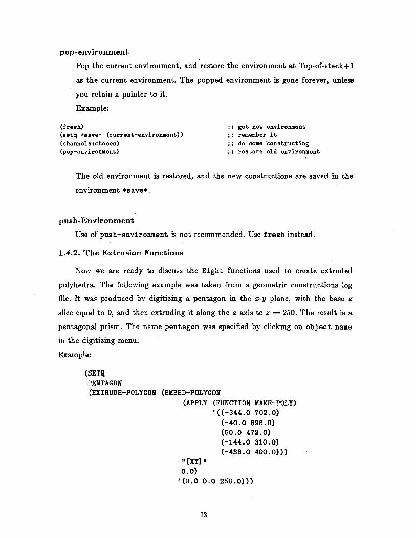
pop-environment

Pop the current environment, and restore the environment at Top-of-stack+1

as the current environment. The popped environment is gone forever, unless

you retain a pointer to it.

Example:

(fresh) ;; get new environment(setq *save* (current-environment)) ;; remember it(channels:choose) ;; do some constructing

(pop-environment) ;; restore old environment

The old environment is restored, and the new constructions are saved in the

environment * save*.

push-Environment

Use of push-environment is not recommended. Use fresh instead.

1.4.2. The Extrusion Functions

Now we are ready to discuss the Eight functions used to create extruded

polyhedra. The following example was taken from a geometric constructions log

file. It was produced by digitizing a pentagon in the x-y plane, with the base z

slice equal to 0, and then extruding it along the z axis to z = 250. The result is a

pentagonal prism. The name pentagon was specified by clicking on object name

in the digitizing menu.

Example:

(SETQPENTAGON

(EXTRUDE-POLYGON (EMBED-POLYGON

(APPLY (FUNCTION MAKE-POLY)'((-344.0 702.0)

(-40.0 696.0)(50.0 472.0)(-144.0 310.0)(-438.0 400.0)))

" [TXY] "

0.0)' (0.0 0.0 250.0)))

The functions used to create the pentagon are as follows: First we make a 2-D

polygon. Next, we embed the polygon in the x-y plane at z = 0. Finally, we

extrude the embedded polygon along the sweep vector (0, 0, 250).

make-poly &rest points

Make and return a two-dimensional polygon out of points. points is a list of

x-y pairs of real numbers. points should not repeat the first point.

embed-polygon poly plane &optional (slice 0.0)

poly must be a 2-D polygon, such as make-poly returns. plane must be a

string which is one of the following: " [XY] ", " [YZ] ", or " [XZ] ". This function

takes a 2-D polygon and returns a 3-D polygon, embedded in a plane parallel

to the specified plane with the value of the excluded axis equal to slice.

Example:

(EMBED-POLYGON(APPLY (FUNCTION MAKE-POLY)

'((-344.0 702.0)(-40.0 696.0)(50.0 472.0)))

" [XY] "500.0)

The 2-D polygon with coordinates { (-344, 702), (-40, 696), (50, 472) } is to be

embedded in a plane parallel to the x-y axis with value z = 500. The returned

3-D polygon has coordinates { (-344, 702, 500), (-40, 696, 500), (50, 472, 500) }.

If the " [XZ] " plane were specified instead, note that the resulting coordinates

would be { (-344, 500, 702), (-40, 500, 696), (50, 500, 472) }.

extrude-polygon poly sweep

Return a solid resulting from sweeping poly along sweep vector sweep. poly

must be a 3-D polygon, such as one returned by embed-polygon. sweep can

be any 3-D vector (a 3-D vector is a list of 3 real numbers). Note that sweep

need not be orthogonal to the plane of poly. The returned structure is of type

solid.

1.4.3. Rotating Solids

To rotate a solid to a new orientation, you use the function Oiler. Oiler

is destructive, i.e., it changes the coordinates of the solid forever. If you want to

preserve a copy of the solid in the old orientation, use copy-complex to copy it

first.

Currently, Oiler employs roll, pitch, and yaw angles to represent rotations.

This may change to Euler angles in the future, or perhaps a new function will be

provided instead3

oiler rotation center object &optional transform

Returns: object, transform. Rotate obj ect as specified by rotation and center.

Return the modified object, and the transformation matrix transform which

was constructed. The operation is destructive-i.e., it modifies object.

rotation is specified as a list of three angles (each angle must be a real

number). center is a 3-dimensional vector specifying the center of rotation,

that is, the center of the local coordinate system about which the rotation

takes place. object may be a structure of type solid or of type face.

If transform is not supplied, then a transformation matrix, as specified by

rotation and center, is constructed. The object is rotated, and returned

along with the transformation.

If you supply transform, however, then it is assumed to be a 4 X 4 transformation

matrix which is applied to object. In this case, rotation and center are

ignored. This facility is provided so you can apply arbitrary transformation

matrices to the objects.

If object is a solid, then oiler will attempt to recompute the plane equations

of obj ect's faces by calling 3d-assign-outward-normals (see below).

3Oiler will rcmain available in sonme form to maintain compatibility.

When you specify a rotation using the digitizing pop-up menu, the following

function is used to compute a default center of rotation:

mock-centroid object

Return the center of mass of the set of vertices of object, treating each vertex

as having unit mass.

1.4.4. Where Coordinate Information is Stored

The transformation functions work by modifying the geometry of the

coordinates of the vertices, while leaving the topology of the polyhedron-the

information about how faces, edges, and vertices connect-intact. Coordinate

information is associated only with vertices. Edges, of course, must point at the

vertices which form their boundary, but to change the coordinates of an edge, we

must obtain its vertices and modify their coordinates. The following functions are

useful in this regard.

0* Note: henceforth, unless otherwise indicated, an object is a structure of type

vertex, edge, face, or solid.

vertices-of object

Return the vertices of object as a list of vertex structures. If object is a

face, then the coordinates are ordered in a loop as they appear on the face.

(Thus for faces, vertices-of returns a sorted list).

all-vertices object

Return the vertices of object as a list of vertex structures. As opposed

to vertices-of, however, make no attempt to order the vertices for faces.

all-vertices is faster when applied to faces and solids.

coordinates vertex Subst

Return the coordinates of vertex. Each coordinate is a 3-D vector.

coordinates-of object

Return the coordinates of all the vertices of obj ect. If obj ect is a face, then the

list of coordinates is ordered as per the face loop. Note that coordinates-of

could have been defined by

(defun coordinates-of (object)(mapcar #'coordinates (vertices-of object)))

2. Experimental Facilities

Eight has facilities for finding the common intersection of two convex polyhedra,

and for constructing the convex hull of two faces in the environment. These are

called experimental facilities because they are not fully debugged.

Even if you are not interested in these facilities, you might want to skim this

chapter, since it presents an example of how to pick objects from the environment

by pointing at a perspective view with the mouse.

2.1. The Intersection Facility

The intersection facility takes as input two convex solids, A and B and

constructs their common intersection, AnfB. A new environment is created, (using

fresh), to which AnB is added. The old environment may be restored via

pop-environment, which can be envoked by clicking on Environment in the Eight

command menu, and then clicking Pop environment in the environment pop-up

menu.

To try out the intersection facility, load the geometric log file "oz:ps:-

<brd>interference-example.lisp, and invoke the Eight command menu via

<function>-D. Click on Operation. The operation pop-up menu will appear. By

default, it is set up to perform an intersection of two solids that you choose by

pointing with the mouse, so you don't need to choose anything on the menu other

than Do it.

In the environment you have loaded, there are two solids that intersect. As you

move the mouse around on the screen over the perspective view, different solids

will be highlighted as you pass over them. Click left with the mouse to indicate

when you have made your selection. You must select two operands-A and B-to

be intersected. The intersection facility will construct An B and draw it for you in

a, new environment.

2.2. The Convex Hull Facility

The convex hull facility takes as input two convex faces fi and f2 from the

environment, and constructs a solid which is their convex hull. The new solid is

added to the current environment. Formally, the new solid is defined as

conv(fi U f2) = conv(vert(fi) U vert(f 2))

where conv(X) denotes the convex hull of a set X, and vert(X) denotes the vertices

of X.

To invoke this facility, click on Operation on the Eight command menu. In

the operation pop-up menu, you can select either the intersection (inter) facility

of the convex hull (conv) facility. Click on conv. By default, the system assumes

input from the mouse. Move the mouse over the perspective view. As you move

over the image of different faces, they will be highlighted as long as the mouse is

inside them. Click left to select a face. When you have selected two faces, their

convex hull will be constructed.

3. How Objects are Represented

It is possible that the extrude facility will prove adequate for your application.

However, there are many kinds of polyhedra which this facility cannot construct.

These solids require a bit more work to build, and require learning something more

about the representations and algorithms Eight employs. These representations

are also used, ultimately, by the extrude facility, and are generally useful to know

about. After mastering this section, you will understand how to build any (finite)

polyhedral object using Eight

3.1. Cells and Complexes

The underlying representation Eight employs is a polyhedral version of the

CW-complex which is a concept from algebraic topology (for example, see (Massey)).

In general, a CW-complex is a space constructed by starting with a graph and

pasting on cells of successively higher dimensions.

The basic notion about all Eight objects is that they may have a boundary.

The boundary of an edge is two vertices. The boundary of a face is an ordered

list of edges. The boundary of a solid is a list of faces.

Coboundary is the dual of boundary. The coboundary of a vertex is the set

of edges which meet at that vertex. The coboundary of an edge is the list of faces

it bounds. The coboundary of a face is the set of 0, 1, or 2 solids it bounds.

Of course, if a face or edge exists in isolation-i.e., is not part of any solid (resp.,

face)-then its coboundary is nil.

A cell is implemented as a structure in Eight , on which all objects (vertices,

edges, faces, and solids) are built. A cell has two basic components, called

boundary and coboundary, which have more or less the intuitive meanings. A cell

is a subtype of every vertex, edge, face, and solid, and thus the boundary and

coboundary accessors can be applied to these objects.

In mathematics, the boundary of a cell k is denoted 8k, and the coboundary

of k is denoted 6k.

boundary cell Subst

Return the boundary of cell. (boundary edge) returns a list of two vertex

structures. (boundary face) returns an ordered list of edge structures defining

the edges bounding face. (boundary solid) returns a list of faces. (boundary

vertex) is undefined.

coboundary cell Subst

Return the coboundary of cell. (coboundary vertex) returns a list of edges

incident at vertex. (coboundary edge) returns a list of faces which edge

bounds. (coboundary face) returns a list of solids which face bounds. Any

of these lists may be nil if the cell does not bound anything. (coboundary

solid) is undefined.

When boundary and coboundary are undefined, they return the atom new:na

(for "not applicable").

Definition: in Eight any collection of cells is called a complez.

Example: a face structure f is a complex comprising f, f's edges, and f's vertices.

Formally, the complex f defines is the set

if}U a U( U ae).eEaf

Note that boundary and coboundary are accessor macros, and hence, if you

need to, you can set them using (setf (boundary face) ... ). You probably

shouldn't do this unless you know what you are doing.

For any cell k, the boundary and coboundary operators keep track of what cells

k bounds, and what cells bound k. For convenience, the following two synonyms

are defined for boundary and coboundary:

a cell Subst

(a cell) = (boundary cell).

6 cell Subst

(6 cell) = (coboundary cell).

This notation is consistent with that of algebraic topology.

Cells are constructed using the following macros:

make-vertex coordinates &optional coboundary

Create a vertex structure with coordinates coordinates (which must be a

3-vector), and coboundary coboundary. If coboundary is not supplied, then

the returned vertex will have null coboundary.

make-edge vO vi &optional (env (current-environment))

Make an edge between vertices vO and vi. vO and vi must be vertex structures.

The edge is added to environment env. The vO and vi are automatically

updated by adding the new edge to their coboundaries. The new edge is

returned.

make/find- existing- edge vO v1 &optional (env (current-environment))

If there is an existing edge betwen vertices vO and vi, then return it. Otherwise,

call make-edge to create a new edge.

Incidentally, to see if there is an edge between vO and vi, evaluate the form

(intersection (coboundary vO) (coboundary vi)).

make-face edges &optional (env (current-environment))

Make a face with boundary edges. edges must be an ordered list of edge

structures. The new face is added to environment env, and is returned. The

coboundaries of each edge in edges are updated.

For make-face to work correctly, the edges must also be contiguous, that is,

consecutive edges must share a vertex, and the first and last edge in the list

must also share a vertex.

make-solid faces &optional (env (current-environment))

Make a solid whose boundary is faces. faces must be a list of face structures.

The new solid is returned, and added to env. The coboundaries of the faces

are appropriately updated to contain the new solid.

Example: Suppose we wish to make the 100 X 100 X 100 cube which we

extruded earlier, using the make- primitives. Note that by varying the vertex

coordinates, any polyhedron topologically equivalent to the cube may be created.

(let ((vO (make-vertex '(0.0 0.0 0.0)))(vi (make-vertex '(100.0 0.0 0.0)))

(v2 (make-vertex '(100.0 100.0 0.0)))(v3 (make-vertex '(0.0 100.0 0.0)))(v4 (make-vertex '(0.0 0.0 100.0)))(v5 (make-vertex '(100.0 0.0 100.0)))(v6 (make-vertex '(100.0 100.0 100.0)))(v7 (make-vertex '(0.0 100.0 100.0))))

(let ((eOl (make-edge vO vi))(e12 (make-edge vi v2))

(e23 (make-edge v2 v3))(e30 (make-edge v3 VO))(e45. (make-edge v4 v5))(e56 (make-edge v5 v6))(e67 (make-edge v6 v7))(e74 (make-edge v7 v4))

(e04 (make-edge vO v4))

(ei5 (make-edge vi v5))(e26 (make-edge v2 v6))(e37 (make-edge v3 v7)))

(let ((fi (make-face (list eOl e12 e23 e30)))(f2 (make-face (list e45 e56 e67 e74)))(f3 (make-face (list eOl el5 e45 e04)))(f4 (make-face (list e12 e26 e56 e15)))(f5 (make-face (list e23 e37 e67 e26)))(f6 (make-face (list e30 e04 e74 e37))))

(setq cube (make-solid '(list fl f2 f3 f4 f5 f6))))))

Whew! Aren't you glad you can use the extrude facility instead? You're

probably wondering why anyone would want to use the cell functions at all. There

are several reasons. First of all, using these operators, you can create any finite

polyhedral object. For example, suppose you wanted to construct two cuboids, with

non-intersecting interiors, and which shared an edge. Note that the coboundary

of this shared edge would contain four faces (two on each cube). To construct the

cubes, you simply use the same edge in constructing the boundary of the faces. Last,

the representation in Eight allows you to use powerful "topological" operators,

which we discuss later. Let's take a detour, however, and discuss how to point at a

perspective drawing and pick out faces and solids with the mouse.

4. Using the Mouse to Select Faces and Solids from a Perspective

View

In the Experimental Facilities chapter (see) we describe systems in which the

user selects faces and solids by moving the mouse over a perspective view of the

environment. As the mouse passes through the image of a face or solid, the object

is highlighted (it blinks) on the screen. A selection is made by clicking left when

the desired object is blinking. The selected object is returned.

This is a useful feature for pointing at objects in the environment without

knowing their names. The function is also available to the user.

mouse-select- entity type &optional who-line-name who-line-message

Select an entity of type type using the mouse, and return it. type must be

:face or :solid. As the mouse is moves over objects of the selected type,

they blink. By clicking left, the blinking object is returned. Middle aborts,

returning new: abort.

Example:

(mouse-select-entity :face "operand 'mustache'")

Allows you to choose a face from the perspective view, with the who-line

message reading something like: "[Choosing operand 'mustache'] Select a face

with mouse. Middle aborts." The function should return a structure of type

face.

Note that if you are calling this function yourself, you should clear the

screen and draw the perspective view first by saying something like (progn

(channels:mapini) (disflush) (draw-edges (get-edges))).

5. More Graphics Functions

Now that you can pick objects off the screen, you're probably wondering how

to draw them. The following functions can help.

channels:plot face

Draw face in perspective on the screen. face must be a structure of type

face.

draw-stars points

points is a list of 3-D points. Draw a small "star", in perspective, where the

point is. draw-stars is useful for pointing out vertices and edges in a drawing.

A finite line in 3-dimensional space may be specified by a list of two 3-D points

(its endpoints). Such a structure is called a line.

draw-lines lines

Draw lines in perspective. lines must be a list of line structures.

draw-flashing forms Macro

Execute forms twice, with tv:alu-xor. Thus forms will draw twice in

exclusive-or drawing mode, causing anything you draw to blink.

Example:

(dotimes (i 6) (draw-flashing (channels:plot face)))

causes face to blink for a while on the screen.

Now, as you write more advanced programs, you will ultimately want to send

your own messages to the graphics windows. The combination of graphics window

and small lisp listener is set up using the function

channels:disini

Set up graphics window and small lisp lisnener.

The relative size of these two windows can be controled using the <function>-E

command. <function>-E selects these two windows. <function>-<n>-E, where

1 < n < 7, selects successively larger lisp windows.

channels:slave-window Variable

The graphics window.

channels:slave-lisp-window Variable

The lisp listener.

You can output text to the graphics window using the function slave-text.

slave-text &rest format-args

Output text, as specified by format-args, to the graphics window.

The following function is a generic drawing facility, which can take a cell of

any type as its argument.

draw-complex cell

Draw cell in perspective. Cell must be a vertex, edge, face, solid, or piano

(see below).

6. Other Eight Functions and Features

6.1. Face Normals

Every face can have a normal, which is actually a four-dimensional vector

(a,b,c, d) representing the plane equation of the face. Thus if (x,y,z) are the

coordinates of a vertex of the face, then ax + by + cz + d = 0.

normal face Subst

Return the normal of face. You can set the normal by (setf (normal face)

You can compute the plane equation of a face using the function

planeq coordinates

Return a four-dimensional vector which is the plane equation of coordinates.

Example:

(setf (normal face)(planeq (coordinates-of face)))

Functions in Eight (and, in particular, hide) assume that faces bounding solids

have normals which point outward. However, if your polyhedra are convex, you can

use the function 3d-assign-outward-normals to automatically assign outward

normals.

3d-assign-outward-normals solid

Assign outward normals to all the faces of solid, which is assumed to be a

convex polyhedron.

Otherwise, if you know a direction which is inside-pointing relative to the face,

you can use

3d-assign-normal face &optional inside-direction set-p

If the normal for face is pointing inside, relative to inside-direction, then

flip it if set-p is T. inside-direction must be a 3-D vector. If the normal is

unknown, planeq is called to compute it.

6.2. Typing

The functions vertex-p, edge-p, face-p, and solid-p return T if their

argument is a structure of that type.

Environments are implemented as instances of the flavor environment:

environment Flavor

6.3. Geometry Functions

The following function is used to translate any object in the workspace.

translate-complex object trans &optional (recompute-normals-p (solid-p ob-

ject))

Translate object by trans. trans must be a 3-dimensional vector. If

recompute-normals-p is T, then call 3d-assign-outward-normals on object

after translating.

Recall that you can rotate a solid or face, and in fact transform it by an

arbitrary 4 X 4 transformation matrix, using the oiler function.

piano Structure

A piano is a collection of solids which is recognized as a valid type by

draw-complex. pianos are useful for representing objects comprising several

polyhedra. The name piano comes from the motion planning literature, where

the moving object is sometimes called a piano.

6.4. Environment Functions

The return-environment command is syntactic sugar for current-environment.

return-environment Macro

Return the current environment.

The defEnvironment form takes a list of objects and creates a new environment

containing them. You can evaluate a series of forms in the new environment, and

the new environment can be returned.

defElVnvironment objects &body forms Macro

Create a new geometric environment, containing objects, and bind the

current environment to it while executing forms. If the last form is (return-

environment), the created environment will be returned.

Example:

(defEnvironment (append (get-faces) (boundary hedron))(channels:choose)

(return-environment))

This form creates and draws a new environment containing the faces in the

current environment, and the faces of polyhedron hedron. Each object is

treated by defEnvironment as a complex, and all cells in the complex are

added to the new environment. (Actually, vertices are not added, since they

are not stored directly in the environment).

If forms are not supplied, then defEnvironment simply returns the new

environment containing objects.

6.5. Property List Functions

A sort of property list capability is provided for objects of type vertex, edge,

face, and solid. This capability uses the properties slot of the cell structure

on which these objects are built. Since all objects are built on the subtype cell,

these functions and accessors may be applied to them.

properties cell Subst

Return the properties of a cell.

assign cell value property-name

Analogous to putprop. Assign property with indicator property-name and

value value to cell. Properties are stored in cell's properties slot.

get-p cell property

Analogous to getprop. Lookup property name property in cell's properties

slot.

rem-p cell property

Analogous to remprop. Remove property property from cell.

The defAccess macro may be employed to dynamically declare additional

"slots" in cell structures. The slots are implemented as properties.

defAccess access-function Macro

Defines a Subst named access-function which is equivalent to:

(defaccess My-slot) =

(defsubst My-slot (object)(cadr (assq 'My-slot (properties object))))

Thus defAccess defines My-slot to be an inverse of assign, in the sense that

after (assign cell value My-slot), (My-slot cell) returns value.

6.6. Utilities

R3-projection vector Subst

Project a four dimensional vector into 3-dimensional space.

(R3-proj ection (a, b, c, d)) = (a, b, c).

homogenize vector

Express a 3-dimensional vector in homogeneous coordinates.

(homogenize (a, b, c))

unhomogenize vector

Given a vector in homogeneous coordinates, return the corresponding 3-space

vector.

(unhomogenize (a, b, c, d)) = ( , , ).

6.7. The Fast Set Package

Many operations in Eight are implemented via set operations. This is because

the geometric model Eight employs allows many geometric computations to be

reduced to purely algebraic operations. The two primitive set operations are set

difference and set intersection. Naive implementations-such as that of the lisp

system-are O(n 2 ). By using hash tables, the fast set package can implement the

intersection of two sets, or the set difference of two sets, in time O(ni + n2), where

nl and n 2 are the size of the sets. These are asymptotic bounds; for small sets with

less than about 100 elements, the Zetalisp functions are generally faster due to the

overhead in allocating the hash tables. Eight employs thresholding, based on the

size of the set, to decide which functions to use.

Sets are implemented as lists.

set-dif A B

Compute the set difference of A and B, that is, A - B, in time O(IAI + JBI).

remove-all B A

Functionally, the same as (set-dif A B), i.e., remove all elements of B

from A. remove-all uses size thresholding: if the size of B is greater than

*set-op-use-hash-table-threshold*, then set-dif is called. Otherwise, a

simple O(IAIBI) tail-recursive remove is performed.

fast-intersection &rest Sets

Return the intersection of Sets, that is, if the sets are A 1,...,A., compute

= (a, b, c, 1).

niA . Takes time O(Et' iAij). For small lists, you should use the system

function intersection, which is O(f[•,.IAiI).

set-partition A B

Compute and return multiple values for A - B, Af B, and B - A.

remdup A

Return set A with duplicates removed; O(IA12).

fast-remdup A

Return set A with duplicates removed; O(JIA). fast-remdup is only worth it

for large lists.

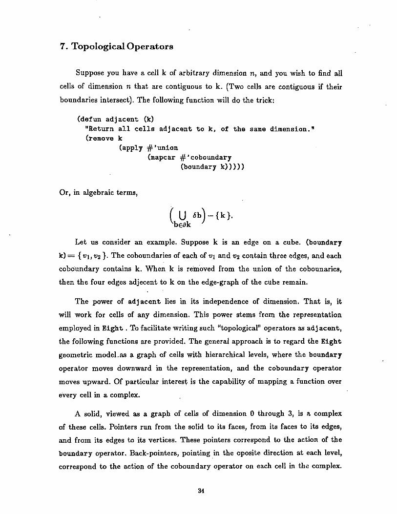
7. Topological Operators

Suppose you have a cell k of arbitrary dimension n, and you wish to find all

cells of dimension n that are contiguous to k. (Two cells are contiguous if their

boundaries intersect). The following function will do the trick:

(defun adjacent (k)"Return all cells adjacent to k, of the same dimension."(remove k

(apply #'union(mapcar #' coboundary

(boundary k)))))

Or, in algebraic terms,

(U 6b)-{k}.bEak

Let us consider an example. Suppose k is an edge on a cube. (boundary

k)= { vl, V2 }. The coboundaries of each of vi and v2 contain three edges, and each

coboundary contains k. When k is removed from the union of the cobounaries,

then the four edges adjecent to k on the edge-graph of the cube remain.

The power of adjacent lies in its independence of dimension. That is, it

will work for cells of any dimension. This power stems from the representation

employed in Eight . To facilitate writing such "topological" operators as adj acent,

the following functions are provided. The general approach is to regard the Eight

geometric model.as a graph of cells with hierarchical levels, where the boundary

operator moves downward in the representation, and the coboundary operator

moves upward. Of particular interest is the capability of mapping a function over

every cell in a complex.

A solid, viewed as a graph of cells of dimension 0 through 3, is a complex

of these cells. Pointers run from the solid to its faces, from its faces to its edges,

and from its edges to its vertices. These pointers correspond to the action of the

boundary operator. Back-pointers, pointing in the oposite direction at each level,

correspond to the action of the coboundary operator on each cell in the complex.

Thus the coboundary pointers run from a solid's vertices to its edges, from its edges

to its faces, and from its faces to the solid itself.

To copy a solid, you must also copy all of its faces, edges, and vertices, and

create a new complex isomorphic to the original. This is the only way to vouchsafe

security against side-effects if the original solid is ever changed. This is the familiar

problem of copying embedded structures in the Lisp world. You can copy a complex

using

copy-complex complez

Return a copy of complex.

Example:

(copy-complex solid)

7.1. Mapcomplex and Star

When we examine exclusively the boundary relation, or exlusively the

coboundary relation on a complex of cells, then the cells are organized in a

tree. The mapcomplex and star functions are used for walking through the tree,

and applying a function to every cell which is met. mapcomplex walks the tree

via the boundary operator, working from higher to lower dimensional cells. The

star operator walks the tree via the coboundary operator, working from lower to

higher dimensional cells. The star operator may be familiar to some readers from

elementary algebraic topology.

7.1.1. Mapcomplex

Mapcomplex regards all cells reachable from its argument via any path of

boundary operators as belonging to the same complex.

mapcomplex complex* Uoptional function type

Map function over all cells in complex* for which the predicate type returns

T. complex* may be any simple complex-i.e., vertex, face, edge, or solid-or

a list of simple complexes. function must be a function of one argument, and

type must be a predicate.

If function is the atom :self, then mapcomplex simply returns all the cells in

complex for which type returns T. type can be the function # 'new: %any-type,

which always returns T. These are the defaults for function and type, if they

are not supplied.

Examples:

Let f be a face. (mapcomplex f) returns the set of cells

{ f }U U(U ae).

Let hedron be a solid. (mapcomplex hedron ) returns all the faces, edges, and

vertices of hedron, as well as hedron itself.

(mapcomplex hedron

#'(lambda (cell)(send channels: slave-lisp-window : clear-screen)(disflush)

(draw-complex cell)(describe cell)

(break))

#'(lambda (cell) (or (edge-p cell) (vertex-p cell))))

This example draws and describes every edge and vertex of hedron, entering

a break loop each time.

Suppose we had a function in-cube? which took a 3-dimensional vector as an

argument, and returned T if the point were inside the 100 X 100 X 100 cube we

constructed earlier. Suppose further that we wanted draw all cells in hedron

which intersected the cube, and to return a list of these cells. This can be done

as follows:

(mapcomplex hedron

#'(lambda (cell)(draw-complex cell)

cell)

#'(lambda (cell)(some (coordinates-of cell)

#' in-cube?)))

As a final example, consider how the macro defEnvironment is defined:

(defmacro DefEnvironment (Objects Abody Forms)(let ((body (or Forms

'((Return-Environment)))))' (let ((get-objects-in-current-environment ,objects))

(in-new-environment(mapc #'(lambda (K)

(mapcomplex K#'(lambda (cell)

(send (current-environment) ':add cell))#'(lambda (c)

(or (edge-p c) (face-p c) (solid-p c)))))get-objects-in-current-environment)

,0body))))

7.1.2. Star

The star operator is in some sense the inverse-or more precisely, the dual-of

the mapcomplex function. While the mapcomplex function descends boundary links,

the star function climbs coboundary links in the graph of cells in a complex.

The star of a complex is a precise notion in algebraic topology, and is defined

as follows:

The Star Operator (Formal Definition)

Let P be a polyhedron. Any cell .k is a face of itself, although it is not a proper

face. A proper face of P must be lower in dimension than P: If an n-dimensional

cell k is on the boundary of P, then we call k an proper n-face of P. Thus edges

are proper 1-faces, and vertices proper 0-faces of a 3-dimensional polyhedron. Let

K be some complex of cells. If k is a n-face of K, then we write K > k. We will

usually assume that a face is a proper face.

Now, let E be some set of cells in K. The star of E (in K) is defined by

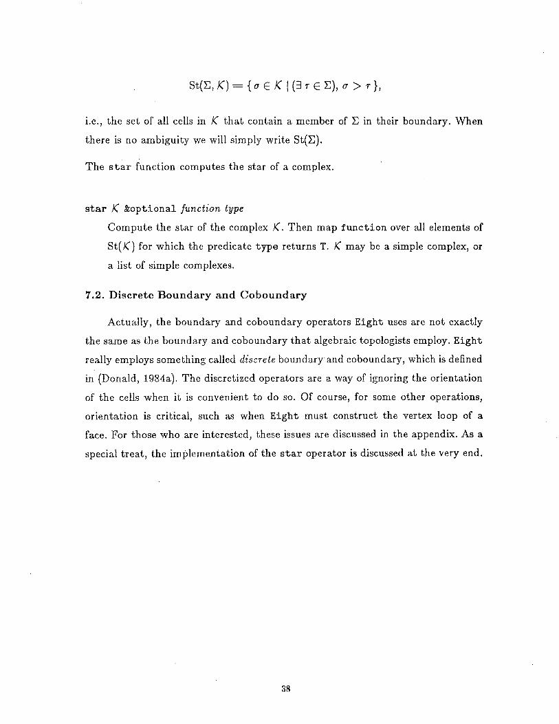
St(E, K)= E K 1 (3 r E ), a > r },

i.e., the set of all cells in K that contain a member of E in their boundary. When

there is no ambiguity we will simply write St(E).

The star function computes the star of a complex.

star K &optional function type

Compute the star of the complex K. Then map function over all elements of

St(K) for which the predicate type returns T. K may be a simple complex, or

a list of simple complexes.

7.2. Discrete Boundary and Coboundary

Actually, the boundary and coboundary operators Eight uses are not exactly

the same as the boundary and cobounidary that algebraic topologists employ. Eight

really employs something called discrete boundary and coboundary, which is defined

in (Donald, 1984a). The discretized operators are a way of ignoring the orientation

of the cells when it is convenient to do so. Of course, for some other operations,

orientation is critical, such as when Eight must construct the vertex loop of a

face. For those who are interested, these issues are discussed in the appendix. As a

special treat, the implementation of the star operator is discussed at the very end.

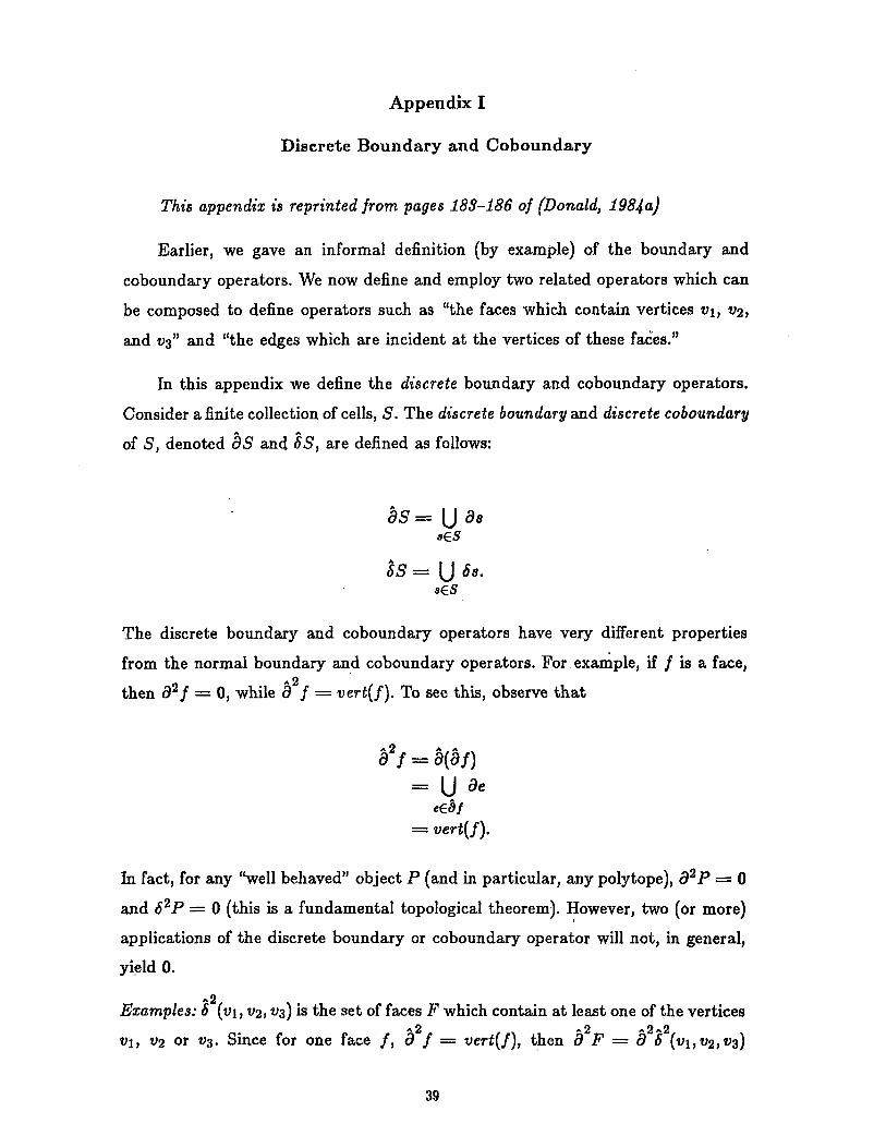
Appendix I

Discrete Boundary and Coboundary

This appendix is reprinted from pages 183-186 of (Donald, 1984a)

Earlier, we gave an informal definition (by example) of the boundary and

coboundary operators. We now define and employ two related operators which can

be composed to define operators such as "the faces which contain vertices vl, v2,

and v3" and "the edges which are incident at the vertices of these faces."

In this appendix we define the discrete boundary and coboundary operators.

Consider a finite collection of cells, S. The discrete boundary and discrete coboundary

of S, denoted aS and 6S, are defined as follows:

as= U assES

6S = U 6s.sES

The discrete boundary and coboundary operators have very different properties

from the normal boundary and coboundary operators. For example, if f is a face,

then a 2f = 0, while a2f = vert(f). To see this, observe that

af = ^(f)

=U ae

= vert(f).

In fact, for any "well behaved" object P (and in particular, any polytope), a2 P = 0

and 62 P = 0 (this is a fundamental topological theorem). However, two (or more)

applications of the discrete boundary or coboundary operator will not, in general,

yield 0.

Examples: 2 (vl, v2, v3) is the set of faces F which contain at least one of the vertices

vl, v 2 or v3. Since for one face f, c f = vert(f), then a2F = -a• (Vl,V 2 ,V3)

is the vertices of all the faces F. The set of edges incident at these vertices is

W3 (v1, v2 , v 3 ).

Exercise: What is 233 (vl, v2, v3 )?

Elementary Review: Boundary, Coboundary, and Star

We must show that the discrete boundary and coboundary operators are well

behaved. We will do so by presenting a formal definition of 0 (and 6) on a single

chain. Readers who have encountered a bit of homology will find the demonstration

transparent. Others may wish to take this section on faith, and to skip to the next

section, where we define the star operator.

Discrete boundary and coboundary operators can be considered as the ordinary

boundary and coboundary "modulo orientation." We see this as follows. (For a

more comprehensive account see any textbook on elementary topology, for example,

Hocking and Young (1961)).

Let K be an arbitrary oriented complex of abstract cells, and Z an arbitrary

(additively written) abelian group. An n-dimensional chain on the complex K with

coefficients in Z is a function cn mapping oriented n-cells of K to Z, such that if

cn(+a n ) = z, then cn(-a n ) = -z. An arbitrary n-chain cn on K can be written as

the formal linear combination

where zi = c,(+au'). The boundary operator 8 is a mapping from n-chains to

(n - 1)-chains. (zi -a') is an (n (n- 1)-chain which has non-zero coefficients only on

the (n - 1)-faces of the cell a'. Formally, let [an, n-1] be the incidence number for

an and on-l, that is

0, if an- 1 is not a face of a n,

[an, n - 1] +l, if an-' is a positively-oriented face of a n ,

-1, if a n - 1 is a negatively-oriented face of an.

Hence,

a(Z -.,)= 0• [,,",,,"-1] • Zi" .- "an--

To factor out the effect of orientation, we define the discrete boundary operator as

follows:

a(z.Q*) = I[,,n, ",-n] .i - .

an-1

Discrete coboundary is defined analogously.

The Star Operator

Let P be a polyhedron. Any cell k is a face of itself, although it is not a proper

face. A proper face of P must be lower in dimension than P: If an n-dimensional

cell k is on the boundary of P, then we call k an proper n-face of P. Thus edges

are proper 1-faces, and vertices proper 0-faces of a 3-dimensional polyhedron. Let

K be some complex of cells. If k is a n-face of K, then we write K > k. We will

usually assume that a face is a proper face.

Now, let E be some set of cells in K. The star of E (in K) is defined by

St(E, K) = { K 1 (3 r E E), a > r },

i.e., the set of all cells in K that contain a member of E in their boundary. When

there is no ambiguity we will simply write St(E). (Giblin (1977), Hocking and Young

(1961)).

For a cell k, define 6ok = k, 5 k = 6k, and 6 k = &(8k), (etc). We see

immediately that the star of { k } may be computed as

St({k })= U] k.i=O

Using this observation, we have implemented the star operator by recording the

boundary and coboundary of each cell in the geometric model.

Appendix I

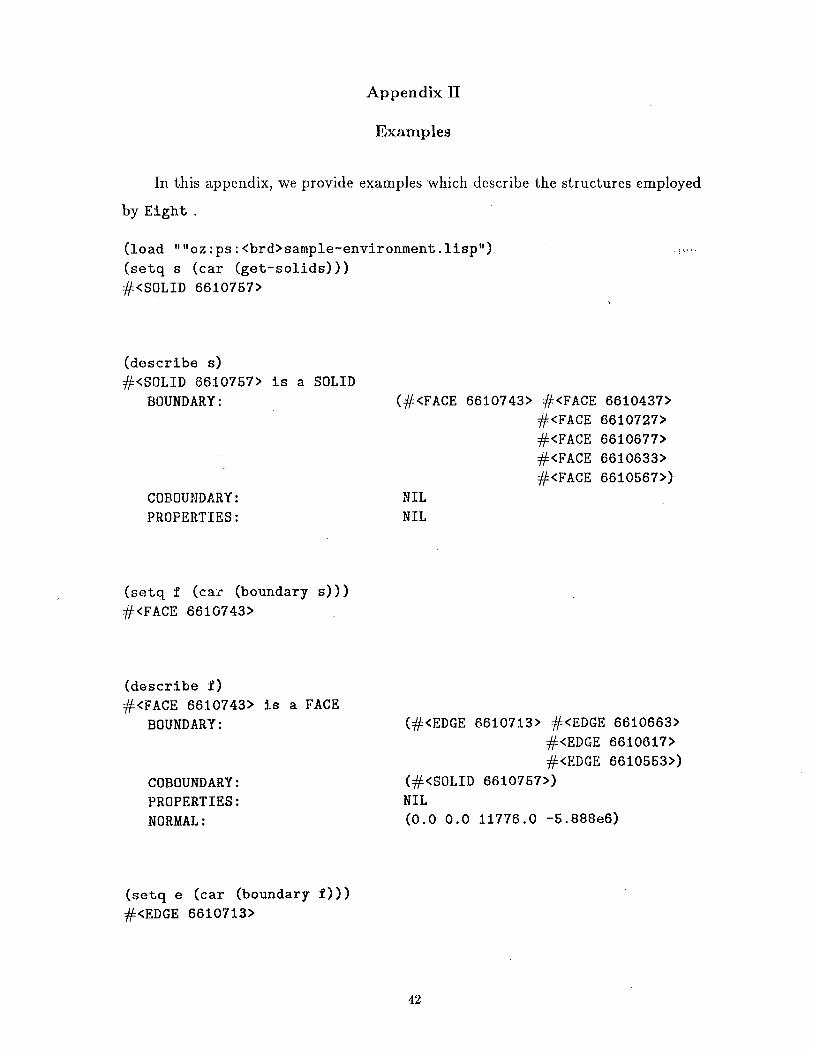
Examples

In this appendix, we provide examples which describe the structures employed

by Eight

(load ""oz:ps:<brd>sample-environment.lisp")

(setq s (car (get-solids)))

#<SOLID 6610757>

(describe s)

#<SOLID 6610757> is a SOLID

BOUNDARY:

COBOUNDARY:

PROPERTIES:

(#<FACE 6610743>

NILNIL

#<FACE

#<FACE

#<FACE

#<FACE

#<FACE

6610437>

6610727>

6610677>

6610633>

6610567>)

(setq f (car (boundary s)))

#<FACE 6610743>

(describe f)

#<FACE 6610743> is a FACE

BOUNDARY:

COBOUNDARY:

PROPERTIES:

NORMAL:

(#<EDGE 6610713> #<EDGE 6610663>

#<EDGE 6610617>#<EDGE 6610553>)

(#<SOLID 6610757>)NIL

(0.0 0.0 11776.0 -5.888e6)

(setq e (car (boundary f)))

#<EDGE 6610713>

(describe e)

#<EDGE 6610713> is a EDGEBOUNDARY:

COBOUNDARY:

PROPERTIES:

(#<VERTEX 6610514> #<VERTEX 6610502>)

(#<FACE 6610743> #<FACE 6610727>)NIL

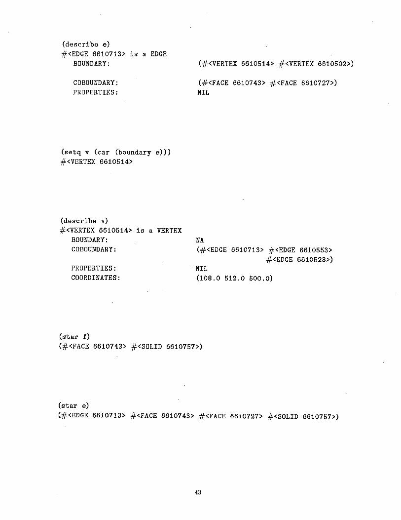
(setq v (car (boundary e)))

#<VERTEX 6610514>

(describe v)

#<VERTEX 6610514> is a VERTEX

BOUNDARY:

COBOUNDARY:

PROPERTIES:

COORDINATES:

NA

(#<EDGE 6610713> #<EDGE 6610553>

#<EDGE 6610523>)NIL

(108.0 512.0 500.0)

(star f)

(#<FACE 6610743> #<SOLID 6610757>)

(star e)

(#<EDGE 6610713> #<FACE 6610743> #<FACE 6610727> #<SOLID 6610757>)

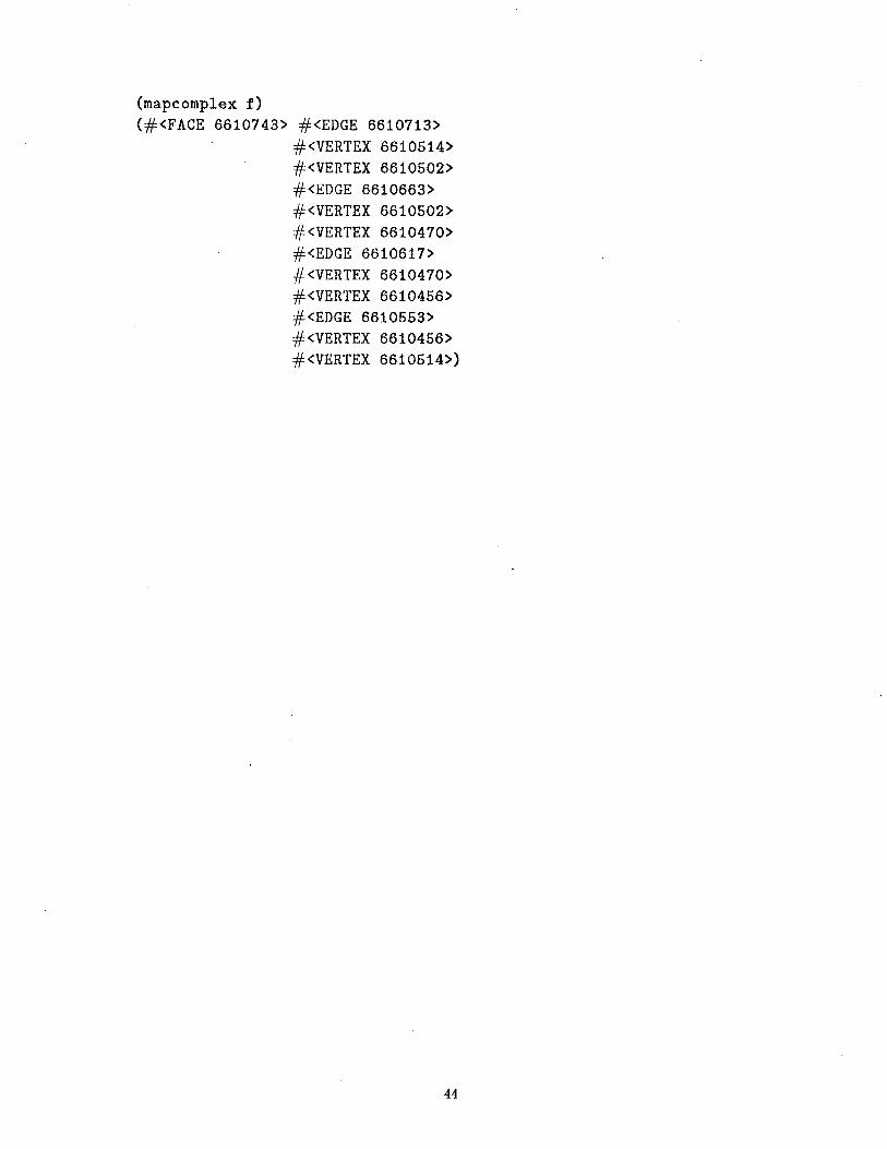
(mapcomplex f)

(#<FACE 6610743> #<EDGE 6610713>

#<VERTEX 6610514>

#<VERTEX 6610502>

#<EDGE 6610663>

#<VERTEX 6610502>

#<VERTEX 6610470>

#<EDGE 6610617>

#<VERTEX 6610470>

#<VERTEX 6610456>

#<EDGE 6610553>

#<VERTEX 6610456>

#<VERTEX 6610514>)

ReferencesBaer, A., Eastman, C., and Henrion, M. "Geometric Modeling: A survey,"

Computer-Aided Design 11, 5 (1979).

Binford, Thomas "Visual Perception by Computer," IEEE Systems Science andCybernetics Conference , Miami, 1971.

Brady, J. M. et al. Robot Motion: Planning and Control, MIT Press, CambridgeiMA, 1983.

Brady, J. M. "Criteria for Representations of Shape," Human .and MachineVision eds. Rosenfeld A., and Beck J., 1982.

Brooks, Rodney A. "Solving the Find-Path Problem by Good Representation ofFree Space," IEEE Transactions on Systems, Man, and Cybernetics SMC-13(1983a).

Brooks, Rodney, A. "Find-Path for a PUMA-Class Robot," AAAI, Washington,DC, 1983b.

Brooks, Rodney A. and Lozano-P6rez, Tomis "A Subdivision Algorithmin Configuration Space for Findpath with Rotations," International JointConference on Artificial Intelligence , Karlsruhe, Germany, 1983.

Burke, G., et al. "The NIL Reference Manual," Laboratory for Computer Science,Massachusetts Institute of Technology, 1983.

Canny, John "On Detecting Collisions Between Polyhedra," European Conferenceon Artificial Intelligence , Pisa, Italy, To be presented October, 1984.

Chatila, Raja System de Navigation pour un Robot Mobile Autonome: Modelisationet Processus Decisionnels, Ph.D. Thesis, L'Universit6 Paul Sabatier de Toulouse,1981.

Chazelle, Bernard "Computational Geometry and Convexity," Department ofComputer Science, Carnegie-Mellon University, CMU-CS-80-150, 1980.

Dobkin, David P. and Kirkpatrick, David G. "Fast Detection of PolyhedralIntersections," Department of Electrical ENgineering and Computer Science,Princeton University, 1980.

Donald, Bruce R. "The Mover's Problem in Automated Structural Design,"Proceedings, Harvard Computer Graphics Conference, Cambridge, July, 1983b.

Donald, Bruce R. "Hypothesizing Channels Through Free-Space in Solving theFindpath Problem," Artificial Intelligence Laboratory, Massachusetts Instituteof Technology, A.I. Memo 736, June, 1983a.

Donald, Bruce R. Local and Global Techniques for Motion Planning, S.M. Thesis,Department of Electrical Engineering and Computer Science, MassachusettsInstitute of Technology, May 10, 1984a.

Donald, Bruce R. "Motion Planning With Six Degrees of Freedom," ArtificialIntelligence Laboratory, Massachusetts Institute of Technology, AI-TR-791, Toappear: August, 1984b.

Drysdale, Robert L. Generalized Voronoi Digrams and Geometric Searching,Department of Computer Science, Stanford University, 1979.

Erdmann, Michael "On a Representation of Friction in Configuration SpaceDuring One-Point Contact (Parts I-II)," "On Motion Planning With Uncertainty,"forthcoming S.M. Thesis, Massachusetts Institute of Technology ArtificialIntelligence Laboratory, 1983.

Foley, J. D. and van Dam, A. Principles of Interactive Computer Graphics,Addison-Wesley, Reading, Mass., 1982.

Forbus, Kenneth D. "A Study of Qualitative and Geometric Knowledge in

Reasoning about Motion," Massachusetts Institute of Technology ArtificialIntelligence Laboratory, AI-TR-615, 1981.

Giblin, P. J. Graphs, Surfaces, and Homology, Chapman and Hall, London, 1977.

Gouzenes, Laurent "Strategies for Solving Collision-Free Trajectories Problemsfor Mobile and Manipulator Robots," Laboratoire d'Automatique et d'Analyse

des Systemes du CNRS, Toulouse, France, 1983.

Griinbaum Convex Polytopes , Interscience Publishers, London, 1967.

Hamilton, W. R. Elements of Quaternions , Chelsea Publishing Co., New York,1969.

Hirsch, M. Differential Topology , Springer-Verlag, New York, 1976.

Hocking, J. and Young, G. Topology, Addison-Wesley, Reading, Mass., 1961.

Hopcroft, J., Joseph, D., and Whitesides, S. "The Movement of Robot ArmsIn 2-Dimensional Regions," Cornell University, 1982.

Kalay, Yehuda E. "Determining the Spatial Containment of a Point in General

Polyhedra," Computer Graphics and Image Processing Vol. 19 (1982), 303-334.

Kane, T.R. and Levinson, D. A.. "Successive Finite Rotations," Journal ofApplied Mechanics 5 (1978).

LCS Mathlab Group "MACSYMA reference Manual, Volumes I-I," The MathlabGroup, Laboratory for Computer Science, Massachusetts Institute of Techno-

logy, 1983.

Lozano-P'rez, Tomas "Spatial Planning: A Configuration Space Approach,"IEEE Transactions on Computers C-32 (February, 1983).

"Automatic Planning of Manipulator Transfer Movements," IEEE Transactions

on Systems, Man, and Cybernetics SMC-11, No. 10 (1981).

Lozano-P6rez, T., Mason, M., and Taylor, R. "Automatic Synthesis of Fine-Motion Strategies for Robots," Massachusetts Institute of Technology Artificial

Intelligence Laboratory, A.I. Memo 759, 1983.

Lozano-Pkrez, T. and Wesley, M. A. "An Algorithm for Planning Collision-Free Paths among Polyhedral Obstacles," Communications of the ACM 22, 10(1979).

Mason, M. T. "Compliance and Force Control for Computer-Controlled Manipulators,"SMC-6 (1981).

Massey, Wm. S. Algebraic Topology, Springer-Verlag, New York, 1967.

Moravec, H. P. "Visual Mapping by a Robot Rover," Proceedings SizthInternational Joint Conference on Artificial Intelligence , Tokyo, Japan, 1979.

Nguyen, Van-Due "The Find-Path Problem in the Plane," Artificial IntelligenceLaboratory, Massachusetts Institute of Technology, A.I. Memo 760, 1983.

Nievergelt J. and Preparata, F. "Plane-Sweep Algorithms for IntersectingGeometric Figures," Communications of the ACM 25, 10 (1982).

Nilsson, Nils Principles of Artificial Intelligence, Tioga Publishing Co., Palo-Alto,1980.

6 'Ddnlaing, C. and Yap, C. "The Voronoi Diagram Method of Motion Planning:I. The Case of a Disc," Courant Institute of Mathematical Sciences, 1982.

6'Duinlaing C., Sharir, M, C. and Yap, C. "Retraction: A New Approach toMotion Planning," Courant Institute of Mathematical Sciences, 1982.

O'Neill, B. Elementary Differential Geometry, Academic Press, New York, 1966.

Paul, L. Robot Manipulation, MIT press, Cambridge, MA, 1981.

Preparata, F. and Hong, S. "Convex Hulls of Finite Sets of Points in Two andThree Dimensions," Communications of the ACM 23, 3 (1977).

Preparata, F. and Muller, D. "Finding the Intersection of n Half-Spaces in TimeO(n log n)," Coordinated Science Laboratory, University of Illinois, Urbana,Ill., R-803, 1977.

Reif, John H. "The Complexity of the Movers Problem and Generalizations,"Proceedings, 20th Symposium on the Foundations of Computer Science , 1979.

Requicha, A. A. G. "Representation of Rigid Solids: Theory, Methods, andSystems," ACM Computing Surveys 12, 4 (1980).

Schwartz, Jacob and Sharir, Micha "On the Piano Movers Problem, I: Thecase of a Two-dimensional Rigid Polygonal Body Moving Amidst PolygonalBarriers," Courant Institute of Mathematical Sciences, Report No. 39, 1981.

Schwartz, Jacob and Sharir, Micha "On the Piano Movers Problem, II: GeneralTechniques for Computing Topological Properties of Real Algebraic Manifolds,"Courant Institute of Mathematical Sciences, Report No. 41, 1982a.

Schwartz, Jacob and Sharir, Micha "On the Piano Movers Problem, III:Coordinating the Motion of Several Independent Bodies: The Special Caseof Circular Bodies Moving Amidst Polygonal Barriers," Courant Institute ofMathematical Sciences, 1982b.

Sechrest, Stuart and Greenberg, Donald "A Visible Polygon ReconstructionAlgorithm," ACM Transactions on Graphics Vol. 1, No. 1 (1982), 25-42.

Spivak, M. A Comprehensive Introduction to Differential Geometry , Publish orPerish, Inc, Berkeley, CA, 1979.

Sutherland, Sproull, et al. "A Characterization Of Ten Hidden-Surface Algorithms,"Acm Computing Surveys 6, 1 (1974).

Symon, K. R. Mechanics , Addison-Wesely, Reading, Mass., 1971.

Udupa, S. Collision Detection and Avoidance in Computer-Controlled Manipul-ators, Ph.D Thesis, Department of Department of Electrical Enginnering,California Institute of Technology, 1977.

Weinreb and Moon "The Lisp Machine Manual," Artificial Intelligence Laboratory,Massachusetts Institute of Technology, 1981.

Widdoes, C. "A Heuristic Collision Avoider for the Stanford Robot Arm," StanfordArtificial Intelligence Laboratory, 1974.

Winston, P. H. and Horn, B. K. P. LISP , Addison-Wesely, Reading, Mass.,1981.

Wittrarn, Martin "A Hidden-Line Algorithm for Scenes of High Complexity,"IPC Business Press 13, 4 (1981).