JOURNAL OF RESEARCH of the Notional Bureau of StandardsVol. 88, No. 2, March-April 1983

The Efficiency of the Biweightas a Robust Estimator of Location

Karen Kafadar*

National Bureau of Standards, Washington, DC 20234

November 9, 1982

The hiweight is one member of the family of M-estimators used to estimate location. The variance ofthis estimator is calculated via Monte Carlo simulation for samples of sizes 5, 10, and 20. The scale factorsand tuning constants used in the definition of the biweight are varied to determine their effects on thevariance. A measure of efficiency for three distributional situations (Gaussian and two stretched-taileddistributions) is determined. Using a biweight scale and a tuning constant of c = 6, the biweight attains anefficiency of 98.2% for samples of size 20 from the Gaussian distribution. The minimum efficiency at n =20 using the biweight scale and c = 4 is 84..%, revealing that the biweight performs well even when theunderlying distibution of the samples has abnormauly stretched tails.

Key words: bisquare weight function; biweight scale estimate; median absolute deviation; M-estimator;tuning constant.

1. Introduction

Robust estimation of location has become an impor-tant tool of the data analyst, due to the recognitionamong statisticians that parametric models are rarelyabsolutely precise. Much discussion has taken place todetermine the "best" estimators ("best" in a certainsense, such as low variance across several distributionalsituations). Estimators which were designed to be robustagainst departures from the Gaussian distribution in. asymmetric, long-tailed fashion were investigated in-depth by Andrews et al. in 1970-1971 [I ].' Subsequent tothis, Gross and Tukey compared several otherestimators in the same fashion, one of which they calledthe biweight [2]. It was designed to be highly efficient inthe Gaussian situation as well as in other symmetric,long-tailed situations. The first reference of its practicaluse appears two years later [31. Gross showed that thebiweight proves useful in the "t"-like confidence intervalfor the one-sample problem [4] and for estimatingregression coefficients [51; Kafadar showed that it is effi-cient for the two-sample problem also [6].

*Center for Appifd Matbematics, National Engineering Laboratory.'igures in brackets indica literature referances at the end of this paper.

Many scientists collect data and perform elementarystatistical analyses but seldom use summary statisticsother than the sample mean and sample standard devia-tion. This paper is therefore addressed to two audiences.It provides a brief introduction to the field of robustestimation of location to explain the biweight in par-ticular (section 2). Those who are familiar with the basicconcepts may wish to proceed directly to section 3 whichraises the specific questions about the biweight's com-putation and efficiency that are answered in this paper.Section 4 describes the results of a Monte Carlo evalua-tion of the biweight. An example to illustrate thebiweight calculation is presented in section 5, followedby a summary in section 6.

2. Robust Estimation of Location;M-Estimates.

Given a random sample of n observations, Xl,...,X ,typically one assumes that they are distributed in-dependently according to some probability distributionwith a finite mean and variance. For convenience, theGaussian distribution is the most popular candidate;representing its mean and variance by St and a', it is wellknown that the ordinary sample mean and samplevariance are "good" estimates, in that, on the average,they estimate 11 and a' unbiasedly and with minimum

105

variance. Often, however, this Gaussian assumption is

not exactly true, owing to a variety of reasons (e.g.,

measurement errors, outliers). Ideally, such departures

from the assumed model should cause only small errors

in the final conclusions. Such is not the case with the

sample mean and sample variance; even one

misspecified observation can throw these estimates far

from the true y and a' (e.g., see Tukey's example in [7]).

It is important, then, to find alternative estimators of

location and scale. Huber 18, p. 5] lists three desirablefeatures of a statistical procedure:

1. reasonably efficient at the assumed model;

2. large changes in a small part of the data or small

changes in a large part of the data should cause

only small changes in the result (resistant);3. gross deviations from the model should not

severely decrease its efficiency (robust).

A class of estimators, called M-estimators, was proposed

by Huber [9] to satisfy these three criteria. This class in-

cludes the sample mean in the following way. Let T be

the estimate which minimizes

£i5 Q(XFT)

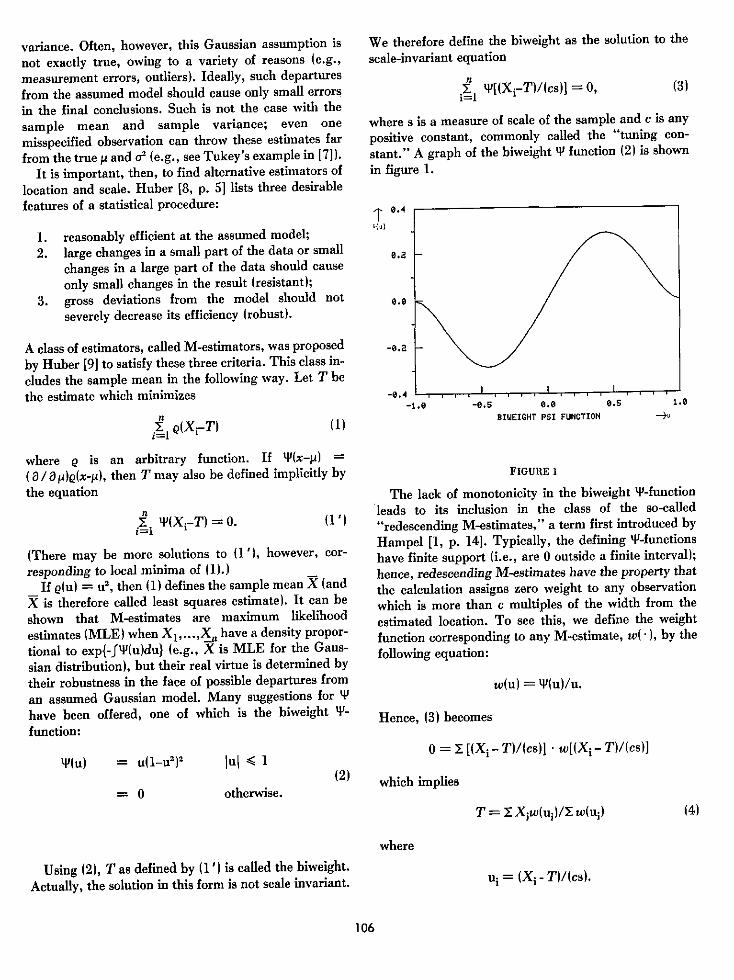
We therefore define the biweight as the solution to the

scale-invariant equation

£Y M'(Xr-T)I(cs)1 0,i=1

(3)

where s is a measure of scale of the sample and c is any

positive constant, commonly called the "tuning con-

stant." A graph of the biweight 4' function (2) is shown

in figure 1.

T 0.4

~0.

0.0

-0.2

-0.4-1.0

(1)

-0.5 0.0BIUEIGI4T PSI FUNCOTION

0.s i.0

where e is an arbitrary function. If 4'(x-p) =

(a/a p)Q(x-A), then T may also be defined implicitly by

the equation

El "UX.T) = O. (I~

(There may be more solutions to (1 1, however, cor-responding to local minima of (1).)

If Q(u) = u2 , then (1) defines the sample mean X (and

X is therefore called least squares estimate). It can be

shown that M-estimates are maximum likelihood

estimates (MLE) when Xl,...,X, have a density propor-

tional to exp{-f t'(u)du} (e.g., X is MLE for the Gaus-

sian distribution), but their real virtue is determined by

their robustness in the face of possible departures from

an assumed Gaussian model. Many suggestions for PV

have been offered, one of which is the biweight 4'-

function:

Y(u) = u(1_u2)2

= O

Jul < I(2)

otherwise.

FIGURE 1

The lack of monotonicity in the biweight 'P-functionleads to its inclusion in the class of the so-called

"redescending M-estimates," a term first introduced by

Hampel [1, p. 14]. Typically, the defining P-functions

have finite support (i.e., are 0 outside a finite interval);

hence, redescending M-estimates have the property that

the calculation assigns zero weight to any observation

which is more than c multiples of the width from the

estimated location. To see this, we define the weight

function corresponding to any M-estimate, w( ), by the

following equation:

w(u) = 'PNu)/u.

Hence, (3) becomes

0 = E [(Xi- T)/(cs)] w[(Xj- T)/(cs)]

which implies

T = Xjw(uj)/X w(uj)

Using (2), T as defined by (1W is called the biweight.

Actually, the solution in this form is not scale invariant. ui = (Xi - Tl/lcs).

106

where

(4)

Equation (4) reveals that the calculation of T may beviewed as an iteratively reweighted average of the obser-vations. A graph of the weight function used for thebiweight,

w(u) (1-u20 2

-O0

constant) part of what would be the corresponding densi-ty (exp(-f Y(u)du)), scaled to have the same density at 0as the unit Gaussian, reveals "shoulders" (Fig. 3), whichmay or may not correspond to realistic applications.

ul! < 1

otherwise, GAUSSIAN DENSITY AND BIUEIGHT 'DENSITY'

0.4

also known as the bisquare weight function, is shown infigure 2, where it is clear that zero weight is assigned toany value outside (To- es, T + es). Henceforth, P and wwill always refer to the biweight M-estimator. I

2~ 0.2

0e

e.e-4 -2 2a 4

DOTTED . GAUSSIAN SOLID - DIUEIGHT C - 4)

SCALED TO MATCH AT X - 0

0.0 L-I.e -2.5 0.0 0.5

BISOUARE UEIGHT FUNCTION

FIGURE 2

Because of the non-monotonicity of the biweight 'Y-function, multiple solutions to (3) are possible. It hasbeen argued that an iteration based on (4) will not con-verge to all of the solutions to (3) and therefore will notget trapped by local minima of (1) [10]. In addition, theiteration suggested by eq (4) is more stable than a rootfinding search suggested by (3). These two facts en-courage the use of (4), called the w-iteration, incalculating T.

3. Use of the Biweight in Practice

There has been considerable discussion on the prac-tical usefulness of the biweight, and of redescending M-estimates in general. Huber points out that they aremore sensitive to scaling (i.e., prior estimation of s in(4)), and warns of possible problems in convergence [8,pp. 102-103]. In addition, unlike the monotone 4'-functions, an estimate defined by a redescending 4'-function is not a maximum likelihood estimate for anydensity function, for it is constant outside a finite inter-val and hence does not integrate to 1. The central (non-

.e Nonetheless. the popularization of the biweightdemands a careful assessment of its performance. Thispaper, therefore, documents its efficiency in threedistributional situations using small- to moderate-sizedsamples.

The study reported below involved a Monte Carlosimulation of three situations, and three sample sizes, inorder to determine the variance of the biweight usingfour different scalings and seven different values of thetuning constant. This section provides details on thecalculation of the biweight, a description of the underly-ing situations in the Monte Carlo study, and the efficien-cy criterion on which it was evaluated.

3.1 Calculation and Scalings

Taking (3) as the definition of T for this study, wecalculate the biweight iteratively: after the kth iteration,

7ft+1 = E Xi W[(Xi -rkl)/(CS)l , k = 0,1,2...T wK(X1 - (5k)/(C8)j

One may begin the iteration with any robust estimate oflocation. For this study, ¶f0) is the median for reasons ofconvenience and computational ease. In this form, thescale estimate remains fixed throughout the iteration.One may also consider updates on the scale:

107

i.e

e.g

0.6

0.2FIGURE 3

(5)

7,+11 = 2I Xi W[UXi - 7 4kl/{jckI1l , k = 0,1,2....I w[(Xi - 74kl)y(cIk)l (6)

Two forms of scale functions were considered in con-nection with iterations (5) and (6). The median absolutedeviation about the current estimate

8MADf k+l) = med I X - I, ' I.4oi1~i'Cn

= med Xi14i'Cn (7)

or "MAD," has been used frequently in manyrobustness studies, including Andrews et al. [1]. In theGaussian situation, the average value of the MAD isroughly two thirds of the standard deviation, so we reallyuse 1.5 x MAD. The second scale is based on a finitesample version of the theoretical asymptotic variance ofT [8, p. 45]:

SUli~l = ( nI sb) PWIn) )1/2

II'1u1)lmax 11, -I + IM''Iujl|

ui = (Xi - rk,/1 csbjikl) . (8)

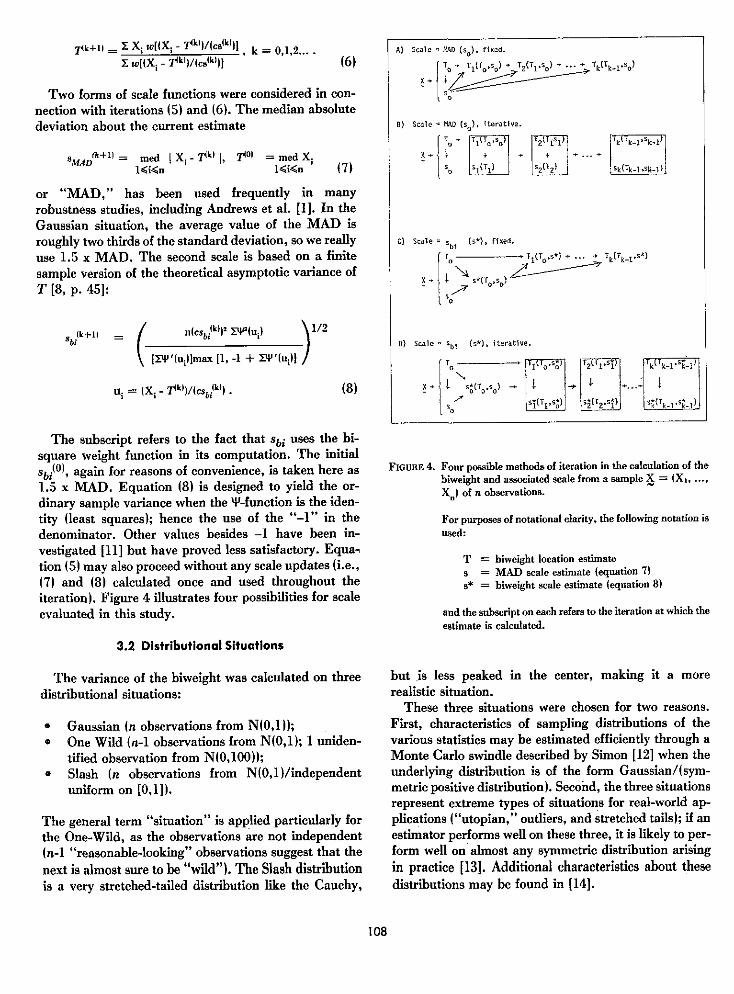
The subscript refers to the fact that sbi uses the bi-square weight function in its computation. The initialsbil0 1' again for reasons of convenience, is taken here as1.5 x MAD. Equation (8) is designed to yield the or-dinary sample variance when the tP-function is the iden-tity (least squares); hence the use of the "-1" in thedenominator. Other values besides -1 have been in-vestigated [11] but have proved less satisfactory. Equa-tion (5) may also proceed without any scale updates (i.e.,(7) and (8) calculated once and used throughout theiteration). Figure 4 illustrates four possibilities for scaleevaluated in this study.

FIGURE 4. Four possible methods of iteration in the calculation of thebiweight and associated scale from a sample X = IX,...

X.) of n observations.

For purposes of notational clarity, the following notation isused:

T = hiweight location estimates = MAD scale estimate (equation 7)s = biweight scale estimate lequation 8)

and the subscript on each refers to the iteration at which the

estimate is calculated.

3.2 Distributional Situations

The variance of the biweight was calculated on threedistributional situations:

* Gaussian (n observations from N(0,1));* One Wild (n-l observations from N(0,1); 1 uniden-

tified observation from N(0,100U);* Slash (n observations from N(0,1)/independent

uniform on [0,1]1).

The general term "situation" is applied particularly forthe One-Wild, as the observations are not independent(n-1 "reasonable-looking" observations suggest that thenext is almost sure to be "wild"). The Slash distributionis a very stretched-tailed distribution like the Cauchy,

but is less peaked in the center, making it a morerealistic situation.

These three situations were chosen for two reasons.First, characteristics of sampling distributions of thevarious statistics may be estimated efficiently through aMonte Carlo swindle described by Simon [12] when theunderlying distribution is of the form Gaussian/(sym-metric positive distribution). Second, the three situationsrepresent extreme types of situations for real-world ap-plications ("utopian," outliers, and stretched tails); if anestimator performs well on these three, it is likely to per-form well on almost any symmetric distribution arisingin practice [13]. Additional characteristics about thesedistributions may be found in [14].

108

A) Scale . AD I ). fixed.

T0 . T(ToD.%) T2(TI -.- So)

0) Sca,= MAD (1). iterative.

so. [qC Tl) sz(T2)k k-15"k 1

C) scale b (s) fixed.

2 +|i (Ts) T1(TsT*(T)k-l-

0) scale *N Sbi ), i:.rative.

2 i t sO(TO'SO) _ l i l l | | ...~~~~~~~~~~~~~~~I- -.....--..

X.1o si(T sO) 1,-T 5L ..... ST t5 1k

T It1)

000~~~~~~~~~~~~~~~~~~~~~~~~~~~~~~~~~~~~~~

3.3 Efficiency Comparisons

In assessing the performance of a location estimator,one typically hopes for (i) unbiasedness, and (ii) minimalvariance. It is simple to see that any M-estimate definedwith an antisymmetric uP function will be unbiased insymmetric situations. Furthermore, Huber has shownthat under some regularity conditions, an M-estimatorhas an asymptotically Gaussian distribution with a finitevariance, even for underlying distributions having in-finite mean and variance [8, pp. 49-501. Thus, it isreasonable to compare the variance of the biweight withthe variance of the unbiased location estimator havingminimal variance, if it exists, for a given situation.

It is known that the minimal variance that is at-tainable for an unbiased location estimator in the Gaus-sian situation is simply I/n, or

Var (Jn X) = VG =1.

Minimal variances for the One-Wild and Slash,however, are not so simple. Theoretically, one mightdetermine the variance of the maximum likelihoodestimate for the One-Wild density but the derivation isnot straightforward. A simple remedy is to pretend thatone knows an observation is wild, which one it is, andeliminate it from the sample. Then the "near-optimal"variance would be

Vw = n/(n-1 ).

A "near-optimal" variance for the Slash density

(l1/o)fz) = [1 - exp(-zt'/2)]/(6/i az2) zoo(2afu11 z=0

where

Z = (X -p)/c,

may be obtained through a maximum likelihood pro-cedure. Details of this derivation may be examined in[15J. The variance of the Slash MLE, Vr, was determin-ed within the Monte Carlo. For all three situations, theefficiency of the biweight is then calculated as

efficiency = "minimum" attainable variancevariance (biweight)

Efficiency as close to I (or 100%) as possible is desirable.So, sometimes it is more useful to calculate the comple-ment, i.e., to examine how far

deficiency = I - efficiency

is from zero (see [1, p. 1211).

4. Results

All computations were performed on a Univac 1108.One thousand samples of sizes 5, 10, and 20 weregenerated. Uniform deviates were obtained using a con-gruential generator [16J; the Box-Muller transform wasapplied to these to obtain Gaussian deviates [171. Theiteration in (4) was terminated when the relative changewas less than 0.0005, or if the number of iterations ex-ceeded 15 (in which case, 1 15 ) became the estimate oflocation).

Tables 1, 2, and 3 provide the variances, their sampl-ing errors (SE) and deficiencies of the biweight for theGaussian, One-Wild, and Slash situations. The most im-mediate observation is the low deficiency of the biweightin the Gaussian situation: using c = 4, as recommendedin Mosteller and Tukey [18], the biweight is never morethan 10 % less efficient than the optimal sample mean forany of the scalings here (except n=5, where it loses 15%for fixed sbi). As c increases, the deficiency is even lower.At c = 6, even for n = 5, the deficiency is less than 6%.As noted by Mosteller and Tukey, relative differences indeficiency of less than 10% are essentially in-distinguishable in practice [18, p. 2061.

Comparing the scalings, Sbi typically provides lowervariances than does 1.5 x MAD. The only exception tothis is in some of the values computed for the Gaussian,where the differences are so small as to be unimportant(at c = 4, largest difference = 4.9%; at c = 6, 2.7%).The differences in deficiency can be quite sizeable for theOne-Wild and Slash situations (e.g., at c = 4, a dif-ference of almost 20% for Slash, n = 20).

In addition, one notes that the additional computationin updating the scale estimate with each iteration is notterribly worthwhile, as deficiencies are only triviallyhigher in most cases. In fact, such updating can causeconsiderable deficiency. As a check on the convergenceof the iteration, table 4 shows the number of samples,out of 1000, that did not satisfy the convergencecriterion. Most of the non-convergences occurred withthe iterative scales, particularly the iterative MAD.

109

TABLE 1. Biweight variances and deficiencies: n =5.

1.5xMAD - Fixed 1.5xMAD - Iterative sbh -Fixed Sb - IterativeTuning Deficiency Deiciency Deficiency DeiciencyConstant Variance SE (%1 Variance SE M%) Variance SE (%) Variance SE M%)

Gaussian (optimal 1.0)

3 1.2114 0.0172 17.5 1.1959 0.0171 16.4 1.2652 0.0203 21.0 1.2475 0.0201 21.1

4 1299 0134 11.5 1065 0130 9.6 1694 0163 14.5 1294 0149 12.65 0879 0109 8.1 0702 0106 6.6 1068 0132 9.6 0816 0126 8.66 0611 0088 5.8 0398 0082 3.8 0693 0106 6.5 0550 0104 6.17 0438 0072 4.2 0200 0053 2.0 0487 0090 4.6 0371 0086 4.4

8 0326 0061 3.2 0155 0045 1.5 0387 0084 3.7 0311 0082 3.8

9 0264 0057 2.6 0124 0043 1.2 0262 0070 2.6 0204 0068 2.6

One-Wild (optimal = 1.2)

3 1.7377 0.0314 30.9 1.7064 0.0302 29.7 1.6946 0.0282 29.2 1.6979 0.0281 30.54 2.0164 0461 40.4 2.1890 0658 45.2 1.8322 0366 34.5 1.9621 0447 40.25 2.4523 0709 51.1 3.0922 1281 61.2 2.1110 0540 43.2 2.5201 0835 53.96 2.9642 0977 59.5 4.2740 1933 71.9 2.6146 0850 54.1 3.3286 1302 65.3

7 3.5080 1235 65.8 5.6037 2657 78.6 3.2118 1199 62.6 4.2358 1748 72.88 4.0822 1481 70.6 6.9447 3101 82.7 3.9072 1537 69.3 5.0837 2163 77.49 4.6817 1725 74.4 8.3881 3705 85.7 4.5843 1877 73.8 5.9725 2561 80.7

Slash (optimal = 10.375)

3 22.291 5.787 53.4 21.964 6.008 52.8 22.497 6.346 53.9 22.312 5.976 63.34 23.470 6.034 55.8 33.974 11.664 69.5 22.618 6.006 54.1 30.965 10.533 75.05 25.218 6.331 58.8 37.209 12.131 72.1 26.191 7.061 60.4 33.872 11.295 77.06 28.207 6.981 63.2 42.045 12.466 75.3 31.643 9.610 67.2 37.952 11.764 79.1

7 31.873 3.205 67.4 45.744 12.647 77.3 34.461 10.723 69.9 39.713 12.034 80.08 34.778 9.289 70.2 47.387 12.743 78.1 37.223 11.570 72.1 42.677 12.312 81.1

9 36.791 10.073 71.8 52.963 13.121 80.4 39.923 12.188 74.0 45.549 12.470 82.1

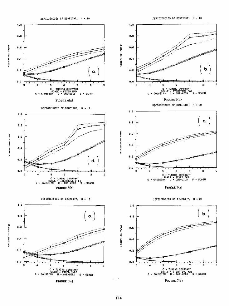
Figures 5, 6, and 7 provide graphs of deficiency as afunction of the tuning constant, for sample sizes n = 5,10, and 20. The uncertainty limits on these graphs, plot-ted with dotted lines, are given by

1 - ["minimum" variance]/[var(biweight) + SE],

where SE refers to the Monte Carlo sampling error in thecalculation of the biweight variances. These reveal that,across these three situations, c = 4 to c = 6 is a practicalvalue of the tuning constant, for larger values tend toyield extremely high deficiencies for the Slash.

The biweight deficiencies computed here scaled by 1.5x MAD (fixed) differ from those computed by Hollandand Welsch [19] in part because of the difference instarting value (they took 'PO) = least absolute deviationsestimate), and in convergence criterion (they took Tes astheir solution). Asymptotically, c = 4.685 yields 95%asymptotic efficiency at the Gaussian [i.e., \/3iT con-

verges in distribution to N(0,1.0526)1; within two sampl-ing errors, the results in tables 1, 2, and 3 are consistentwith this value.

As noted earlier, 115) became the estimate of locationin cases of non-convergence in the study. This only in-creases the variance of the biweight that we are likely tosee in practice, because this situation occurred typicallywhen the iteration alternated between two equally dis-tant values from M. In practice, one should examine thesample to determine the cause of non-convergence, andpossibly settle on the median and 1.5 x MAD as expe-dient location and scale estimates.

5. An Example

To illustrate the calculation of the biweight, we usesome chemical measurements collected at the NationalBureau of Standards. These data were taken from

110

TABLE 2. Biweight variances and deficiencies. n=1 0.

1.5xMAD - Fixed 1.5xMAD - Iterative s .- Fixed s- IterativeTuning Deficiency Deficiency Deficiency DeficiencyConstant Variance SE 1%M Variance SE (%) Variance SE 1%M Variance SE Ml

Gaussian loptimal = 1.0)

3 1.1250 0.0109 11.1 1.1083 0.0115 9.8 1.1937 0.0146 16.2 1.1930 0.0156 16.24 .0578 0075 5.5 0469 0069 4.5 0961 0099 8.8 0800 0083 7.45 0319 0056 3.1 0236 0051 2.3 0479 0068 4.6 0335 0048 3.26 0198 0043 1.9 0133 0035 1.3 0259 0048 2.5 0145 0032 1.47 0126 0031 1.2 0074 0026 0.7 0145 0034 1.4 0056 0013 0.68 0084 0024 0.8 0039 0017 0.4 0078 0023 0.8 0037 0013 0.49 0059 0019 0.6 0029 0019 0.3 0042 0015 0.4 0027 0013 0.3

One-Wild (optimal = 1.1111)

3 1.2785 0.0116 13.1 1.2781 0.0114 13.1 1.3414 0.0161 17.2 1.3413 0.0168 17.24 1.2946 0109 14.1 1.3105 0117 15.2 2709 0112 12.6 1.2630 0105 12.05 1.3714 0137 19.0 1.4125 0159 21.3 2775 0104 13.0 1.2828 0102 13.46 1.4990 0189 25.9 1.5948 0246 30.3 3257 0115 16.2 1.3794 0141 19.47 1.6793 0253 33.8 1.8333 0332 39.4 4196 0163 21.7 1.5757 0242 29.58 1.9034 0331 41.6 2.1332 0445 47.9 5621 0223 28.9 1.9037 0397 41.69 2.1590 0420 48.5 2.4703 0580 55.0 7562 0301 36.1 2.3703 0591 53.1

Slash (optimal = 5.9843)

3 7.0895 0.2795 15.6 7.4991 0.3348 20.2 6.4815 0.2422 7.7 6.5367 0.2465 8.54 7.9896 3382 25.1 8.6854 0.4129 31.1 7.1538 .2796 16.3 7.6037 0.3339 21.35 8.9977 4355 33.5 10.819 0.9005 44.7 8.0679 3586 25.8 9.2930 0.7666 35.66 10.261 5815 41.7 14.567 1.4310 58.9 8.9836 4739 33.4 11.167 0.8863 46.47 11.487 7135 47.9 25.156 8.6783 76.2 10.555 7319 43.3 22.739 7.8504 73.78 12.692 8214 52.8 28.036 9.0950 78.6 11.705 5120 51.6 28.258 8.5066 78.89 13.999 9294 57.3 33.752 9.4908 82.3 12.908 6051 58.4 31.727 8.9310 81.1

several ampoules of n-Heptane material at NBS betweenMay 22 and June 17, 1981. The ampoules were filledfrom two lots in several sets. Lot A includes 20 sets ofampoules; lot B includes six sets; only the data from 10ampoules in sets from lot A will be used here. Panel A oftable 5 shows the mean percent purity from 10 am-poules, where the mean was calculated as an average ofanywhere between 5 and 10 measurements. To eliminatethe big numbers and decimal points, we subtract99.9900 and multiply by 101 in the third column.

Notice that, by virtue of the central limit theorem, onewould expect that these averages would be approximate-ly normally distributed and a higher value for the tuningconstant, say c =5, would be reasonable. The third col-umn of Panel A reveals three somewhat anomolousvalues: -20, 56, and 28. Notice that the low value cor-responds to ampoules in set 21 and the high value tothose in set 20. Since the sets were filled sequentially,there may have been some aspect of the filling procedure

which caused these odd values. Also, the data are listedin the order in which they were measured, so the lowvalue for the first ampoule may have resulted from someproblem in the measuring equipment on the first day.

The iteration initiates with the median, TPO = 7, andSbi is calculated from the median and 1.5 x MAD(= 12.0), yielding a scale estimate of 17.2. The con-vergence criterion in this calculation is relative to theestimated scale; i.e., the iteration ceases when either k >Ž15 or I1 1k) - pk-l)I/sb, 4 .0005.

Panel B gives the bisquare weights associated witheach observation and the biweight at each iteration.Notice that the three "suspect" values all receive lowerweight than the other seven. The final scale estimate,0.0019, is computed from the final location estimate,99.9907, and the Sbi used throughout the iteration(.0017). These estimates compare favorably with thesample mean and standard deviation, 99.9910 and0.0021.

ill

TABLE 3. Biweight variances and deficiencies: n=20.

1.5xMAD - Fixed 1.SxMAD - Iterative sbi - Fixed s - IterativeTiuing Deficiency Deficiency Deficiency DeficiencyConstant Variance SE 1%) Variance SE (%) Variance SE (%1 Variance SE 1%1

Gaussian (optimal = 1.0)

3 1.0973 0.0076 8.8 1.0841 0.0069 7.8 1.2111 0.0147 1?.4 1.2159 0.0154 17.84 0369 0039 3.6 0299 0034 2.9 .0842 0064 7.8 0769 0051 7.15 0172 0026 1.7 0117 0013 1.2 0387 0036 3.7 0331 0024 3.26 0087 0015 0.9 0056 0007 0.6 0187 0019 1.8 0163 0015 1.67 0047 0008 0.5 0030 0004 0.3 0096 0010 0.9 0084 0003 0.88 0027 0005 0.3 0018 0002 0.2 0052 0005 0.5 0045 0004 0.49 0017 0003 0.2 0011 0001 0.1 0030 0003 0.3 0027 0002 0.3

One-Wild (optimal = 1.0526)

3 1.1597 0.0077 9.2 1.1494 0.0055 8.4 1.2663 0.0148 16.9 1.2561 0.0139 16.24 1313 0040 7.0 1298 0037 6.8 1517 0066 8.6 1421 0053 7.85 1572 0049 9.0 1594 0050 9.2 1198 0034 6.0 1185 0034 5.96 2082 0069 12.9 2145 0071 13.3 1273 0037 6.6 1289 0037 6.87 2745 0094 17.4 2848 0097 18.1 1522 0047 8.6 1578 0050 9.18 3532 0122 22.2 3721 0127 23.2 1905 0062 11.6 2019 0067 12.49 4439 0151 27.1 4690 0159 28.3 2431 0081 15.3 2700 0092 17.1

Slash (optimal = 5.2666)

3 6.2724 0.2046 16.0 6.4046 0.2284 17.8 5.6057 0.1410 6.1 6.7146 0.1541 7.84 7.5085 3189 29.9 8.1706 0.4386 35.5 6.2212 1976 15.3 6.4293 0.2137 18.15 8.8490 4364 40.5 10.255 0.6849 48.6 7.3065 2822 27.9 8.3053 0.4552 36.66 10.157 5377 48.1 12.260 0.8502 57.0 8.6312 4237 39.0 10.434 0.6585 49.57 11.453 6307 54.0 13.964 1.0004 62.3 10.116 5670 47.9 12.580 0.8205 58.18 12.733 7235 58.6 15.762 1.1107 66.6 11.832 7166 55.4 15.324 1.0068 65.79 13.996 8083 62.3 17.100 1.1866 69.2 13;442 8405 60.8 18.235 1.1790 71.1

In this case, there is little difference between the twoprocedures, and either may be reported. Had there beena substantial difference, one would want to examine thedata more closely to understand the reason. This is animportant step in data analysis, and robust methods of-fer easy, objective procedures for making this com-parison and illustrating possible anomolies in the data.

6. Conclusions

This paper establishes the variance of the biweight asa location estimator across three distributional situations,for small to moderate sample sizes. In terms of scaling,sbi performs more satisfactorily than does 1,5 x MAD,and need not be recalculated with subsequent iterations.

Three to six iterations of the w-iteration are typically re-quired to attain satisfactory convergence (< .0005 x SO-The minimum efficiencies of the biweight across the threesituations for sample sizes, 5, 10, and 20 at c = 4 are 46%,83%, and 85% respectively; atc = 6 they are 33%, 67%,and 61% respectively. Gaussian efficiencies are con-siderably higher: at c = 4, 86%, 91%, and 92%; at c= 6, 94%, 97%, and 98%.

A final comment concerns the results on n = 5. Forsuch a small sample size, it is encouraging that thebiweight (c = 4) is only 14% less efficient than the op-timal sample mean if the underlying population is reallyGaussian. In fact, Sbi can be very misleading in a small(between 2% and 5% for the situations listed here) butinfluential proportion of the time. Conditioning on someancillary statistic, such as the average value of the weights,would undoubtedly increase the efficiency for all threesituations when n = 5.

112

I.e

TABLE 4. Number of samples (out of 1000 samples of sizen=5/n=l0/n=20) that did not converge (k > 15 and >S+l >

.0005 X scale).

(Tuming 1.SxMAD 1.5xMAD sbi SbiConstant) FIXED ITERATIVE FIXED ITERATIVE

Gaussian3 6/0/0 106/44/9 1/0/0 34/13/04 9/0/0 92/ 5/1 1/0/0 0/ 6/15 1/0/0 68/ 8/2 1/0/0 0/ 2/06 5/0/0 S0/ 4/0 0/0/0 0/ 2/07 3/0/0 33/ 2/0 1/0/0 0/ 0/08 2/0/0 29/ 2/0 0/0/0 0/ 0/09 0/0/0 20/ 2/0 0/0/0 0/ 0/0

One-Wild3 3/0/0 120/ 11/ 6 0/0/0 18/13/ 04 1/0/0 168/ 14/ 3 0/0/0 0/10/ 35 1/0/0 170/ 42/ 0 0/0/0 0/ 9/ 06 0/0/0 159/ 70/ 3 0/0/0 0/47/ 07 1/0/0 138/ 91/ 6 0/0/0 0/46/ 08 0/0/0 121/113/20 0/0/0 0/36/ 09 0/0/0 92/120/37 0/0/0 0/22/32

Slash3 4/0/0 119/31/20 1/0/0 0/ 0/154 5/0/0 156/33/16 0,0/0 1/ 3/155 1/0/0 138/51/24 0/0/0 0/ 0/416 8/0/0 121/81/36 1/0/0 0/ 0/947 1/0/0 99/65/39 1/0/0 0/ 0/568 0/0/0 79/64/48 0/0/0 0/ 0/769 0/0/0 67/53/53 0/0/0 0/32/74

I

IC

0.s

0.I

0.2

0.0

DEF11'NOICES OF BIWE19HT, N . ;

3 4 S 6 7 6 9

SCALE - ITERATIVE lbDFIGURE 5(b)

DEFICIENCIES OF BIUEIGHT, N . 5

i.e

0.9

ICECNC

0.6

0.4

0.2

*.e3 4 S 6 7 a S

TUNING CONSTANTSCALE . FIXED S-BI

FIGURE 5(c)DEFICIENCIES OF BIUEIGHT, N * S

4 5 6 7 a 9C . TUNING CONSTANT

SCALE - FIXED HADG - GAUSSIAN U * ONE-WILD S * SLASH

DEFICIENCIES OF 3IWEIGHT. N . S

3 4 S 6 7

TUNING CONSTANTSCALE - ITERATIVE S-RI

FIGURE 5(d)

I.e

e.s

G.e

0.4

0.2

0.0

0.E

e.g

a.sI

I

HE

CV

3

0.2

e.g

FIGURE Sla)

a 9

113

DEFICIENCIES OF BIUEIGHT. N . 12

4 S 6 7 a

C - TUNING CONSTANTSCALE FIXED MAD

C . GAUSSIAN . * ONE-UILD S - SLASH

FIGURE 6(a)

DEFICIENCIES OF B31EIGHT, N . IJ

4 5 6 7 8C - TUNING CONSTANT

SCALE ' ITERATIVE S-B1G - GAUSSIAN U - ONE-~UILD S * SLASH

FIGURE 6(b)

DEFICIENCIES OF DIWEIGHT, N * 10

I .J

be.

0.8

DFT 0.6F

C

II.

E 0.4

CV

0.2

0.0

1.0

0.8

E 0.6F

CI 0.4NCV

0.2

0.0

D

1.0

0.3

D 0.6F

CIE 0.4NCV

0.2

0.0D

a 4 5 6 7 aC . TUNING CONSTANT

SCALE . ITERATIVE MADG * GAUSSIAN U - ONE-WILD S * SLASH

FIGURE 6(d)

DEFICIENCIES OF BIUEIGHT, N * 20

4 5 6 7 aC . TUNING CONSTANT

SCALE * FIXED MADG . GAUSSIAN U - ONE-WILD S - SLASH

FIGURE 7(a)

DEFICIENCIES OF BIWEIGHT, N . 20

3

3 4 5 6 7 6C . TUNING CONSTANT

SCALE - ITERATIVE MADG F GAUSSIAN U * ONE-WILD S * SLASH

'FIGUIRE 7fh)

114

3

1.0

0.8

DE 0.6F

C

E 0.4NCV

0.2

0.0

i.J

0.8

Dc 0.6F

C

E 0.4NCV

0.2

0.0

i.e

0.8

DJ 0.6

F

CIE 0.4NC

0.2

0.0

39

4 5 6 7 8

C . TUNING CONSTANTSCALE * FIXED S-SI

G . GAUSSIAN U . ONE-WILD S - SLASH

FIGURE 61c)

G

DEFICIENCIES OF BIUEIGNT. N * 10

DEFICIENCIES OF BIWEIGHT. N * 20

3 4 5 6 7C - TUNING CONSTANTSCALE . FIXED S-DI

G - GAUSSIAN U * OME-UILD S * SU

TABLE 5. Measurements on ampoules of n-Heptane.

A) The data

G. ) Set No.-Ampoule

2-053-04

20-207-07

20-0314-102-156-14

a 9 ~~~14-207-17

4SH

% purity

99.988099.990999.995699.990899.990199.992899.991599.989999.990699.9894

(% purity-99.99) 10'

-209

5681

2815

-L6

-6

B) Biweight iterations: c=5, ro)=7.0, sf')=12.0, shi=17.2

Columns give weights w.ik) corresponding to each observation yi at khditeration. '4k) = -Ewjk)y,/Ewki'

DEFICIENCIES OF BEtEIGHT, N . 20

4 5 6 7 8 9C - TUNING CONSTANT

SCALE _ ITERATIVE S-6IF - GAUSSIAN U * ONE-WILD S - SLASH

FIGURE 7(d)

obsv'n

-209

56812815

- 16

- 6

(1)

.8120

.9989

.4546

.9997

.9903

.8839

.9827

.9827

.9997

.9547

(2)

.8082

.9992

.4597

.9999

.9893

.8869

.9839

.9815

.9996

.9527

(3)

.8075

.9992.4606.9999.9891.8875.9841.9812.9995.9523

(4)

.8074

.9993

.4607

.9999

.9891

.8876

.9842

.9812

.9995

.9523

All=,7 28 3 r21=7.334 r"1=7a344 P41=7.345

Final location and scale estimates (original scale):

u = 99.9900 + 7.346/10' = 99.9907o = 18.648/101 = .0019

7. References

[11 Andrews, D.F.; Bickel, P.J.; Hampel, F.R.; Huber, P.J.; Roges,W.H.; and Tukey, J.W. (1972). Robust Estimates of Location:Survey and Advances, Princeton University Press: Princeton,New Jersey.

[21 Gross, A.M., and Tukey, J. W. The estimators of the PrincetonRobustness Study. Technical Report No. 38, Series 2, Depart-ment of Statistics, Princeton University, Princeton, New Jersey.

131 Beaton, A.E., and Tukey, J.W. (1974). The fitting of power series,meaning polynomials, illustrated on band-spectroscopic data.Technometrics 16, 147-185.

[41 Gross, Alan M. (1976). Confidence interval robustness with long-tailed symmetric distributions. J. Amer. Statist. Assoc. 71,409-417.

[51 Gross, Alan M. (1977). Confidence intervals for bisquare regres-sion estimates. J. Amer. Stat. Assoc. 72, 341-354.

[61 Kafadar, K. (1982b). Using biweights in the two-sample problem.Comm. Statist. 11(17), 1883-1901.

[71 Tukey, J.W. (1960). A survey of sampling from contaminateddistributions. In Contributions to Probability and Statistics, 1.Olkin, ed., Stanford University Press, Stanford, California.

[81 Huber, P. (1981). Robust Statistics. Wiley: New York.

[91 Huber, P. (1964). Robust estimation of a location parameter. Ann.Math. Statist. 35, 73-101.

[10[ Lax, D. (1975). An interim report of a Monte Carlo study of robustestimates of width. Technical Report No. 93, Series 2, Depart-ment of Statistics, Princeton University, Princeton, New Jersey.

115

i.e

0.0

0.6

0.4

0.2

0.0

FIGURE 7(c)

1.0

0.8

D£FIC

E

CV

0.6

0.4

0.2

0.0

(5)

.8074

.9993

.4608

.9999

.9891

.8876

.9842

.9812

.9995

.9523

5f=7.346sbi=18.648

3

Jill Tukey, J.W.; Braunt, H.., and Schwarzchild, M. (1977). Fur-ther progress on robust/resistant widths. Technical Report No.129, Series 2, Department of Statistics, Princeton University,Princeton, New Jersey.

[121 Simon, G. (1976). Computer simulation swindles with applicationsto estimates of location and dispersion. Appl. Statist. 25,266-274.

[131 Tukey, J.W. (1977). lecture Notes to Statistics 411. Unpublish-ed manuscript, Princeton University, Princeton, New Jersey.

[14] Rogers W.F., and Tukey, J.W.(1972).Understandingsomelong-tailed symmetrical distributions. Statistica Neerlandica 26, No.3, 211-226.

[151 Kafadar, K. (1982 a). A biweight approach to the one-sample pmob-lem. J. Amer. Stat. Assoc. 77, 416-424.

[161 Kronmal, J. (1964). Evaluation of the pseudorandom numbergenerator. J. Assoc. Computing Machinery, 351-363.

[171 Box, G.E.P., and Muller, M. (1958). A note on generation of nor-mal deviates. Ann. Math. Stat. 28, 610-611.

[181 Moteller F., and Tukey, J.W.(1977). DataAnalysisandRegres-sion: 4 Second Course in Statistics. Addison-Wesley; Reading,Massachusetts.

[191 Holland, P.W., and Welsch, R.E. (1977). Robust regression usingiteratively reweighted least squares. Comm. Statist. A6(9),8134827.

116