The Effects of Near and Far Visual Occlusion upon a Simulated Driving Task

A Master's Thesis by

Jason Myers B.S., South Dakota State University, 1998

December 3, 2002

Abstract

There is a growing body of evidence to suggest that steering behavior during

driving can be described as two separate functions: one based upon closed-loop sampling

of near-range visual information and the other based upon an open-loop anticipatory

utilization of far-range visual cues. Past research has been performed using diagnostic

measures of steering performance that may not be ideal for the separate measurement of

these different mechanisms mediating driver steering performance. Through the use of a

visual occlusion technique to isolate the availability of near-range versus far-range visual

information, the proposed study hoped to demonstrate that RMS error and time-to-line

crossing (TLC) statistics represent relatively independent measures of the near-range and

far-range visual processes, respectively. Results of this investigation supported the idea

that near-range visual processes are indexed by RMS error measurements but failed to

find evidence supporting the idea of a separate far-range visual system for anticipatory

maneuvers using time-to-line-crossing (TLC) as a measure.

2

Introduction

The task of lane-keeping in a car may seem simple and intuitive, yet developing a

full understanding of just how this process works is more complex than it seems. Broken

down into its simplest elements, lane keeping requires maintaining a car on its proper

course and in the proper lane. While this objective seems simple enough, analyses of eye

glance patterns have revealed that drivers use two independent, but complementary,

behavioral mechanisms to guide steering behavior (e.g., Gordon, 1966; Land and Lee,

1994). In fact, Donges (1978) has proposed a comprehensive dual-process model of

automobile steering behavior: the first process consists of a closed-loop monitoring task

using near-range visual input while the second process involves an open-loop

anticipatory analysis of far-range visual information.

Traditional measures of steering behavior have emphasized the first process of

steering by focusing upon the information provided by rear-range edge lines. By using

these edge lines as a guide, experimenters can then quantify the steering behavior by

using RMS lateral position error. This is the vehicle’s Root Mean Squared error, or, the

standard deviation from the center of the road. RMS lateral error accrues as the vehicle

moves from side to side in the lane.

Although, traditionally we would use RMS error to assess driver performance

there is a basic limitation to the information captured by this measure. That is, while

RMS lateral error seems to be a good measure of the short-range steering process there is

evidence that it may be entirely insensitive to far-range visual inputs to driving behavior.

3

In order to fully understand the relationship between edge line visibility and steering

performance we would need to measure beyond the short-range process. Another way to

quantify steering performance is to measure the time-to-line crossing (TLC) statistic.

This is a more recent means of analysis proposed by Godthelp (1984) that can be used to

make predictions about where the vehicle is headed. TLC is the point in the future path

of the vehicle at which time the vehicle will cross the edge line of the road. As such,

TLC appears to represent a good candidate measure for capturing the output of the far-

range steering process.

The concept of a two-component model of driver steering behavior is not a new

one. The origins of this concept can be traced at least back to Gordon’s work in 1966.

Donald Gordon set up an experiment in which drivers were given a very restricted view

of the roadway. In this experiment the drivers wore a helmet with a small vision aperture

that only allowed 4 degrees of view in a fixation. Using a helmet-mounted camera

calibrated with the same small, restricted viewing area as the aperture, Gordon was able

to fashion a rudimentary eye-tracking device. Using this small viewing area in

conjunction with video recording equipment Gordon was able to ascertain where in the

visual scene the drivers were fixating and to break these fixation areas into sections. This

pioneering work was the first to show that drivers used the road edges and the centerline

as their primary source of guidance information. Without the presence of peripheral

information Gordon found that approximately 97% of drivers fixations were on edge

lines or the centerline. Gordon also found evidence for a far-range visual process. The

far-range process may have been underestimated in this study. The original study was

4

done at slow speeds and later findings would indicate that as drivers increase speeds they

tend to look farther down the road for information. This study was done to try to

determine the minimum requirements for effective roadway markings.

This is a question that plagues highway engineers even today, some 35 years later.

Back in Gordon’s study the question was, “How important are edge line markings?”

Today we might ask, “How bright do edge line markings need to be?” The task of

nighttime driving is inarguably more demanding than daytime driving. In the night

driving environment, the driver’s forward view is limited to the reach of his/her vehicle’s

headlights. Even with the best headlights, if the edge lines of the road are too dim the

drivers steering task becomes more difficult as they lose forward information (i.e., as

inputs to the far-range process become attenuated).

In Donge’s two-component model the two levels of the steering process were

termed the guidance level (far range process) and the stabilization level (short-range

process). At the guidance level, the driver extracts information about the present and

future course of the road from the visual field. Donges described this type of information

as the anticipatory, or preview, level. In this level of open loop steering, the drivers are

obtaining information about the desired path of the automobile. Donges dual level model

was created before the concept of TLC; thus, he measured the far-range visual process by

using the curvature of the vehicle’s path to estimate the equivalent forcing function in a

“path neglecting” tracking model.

5

There is another type of information suggested by Donges and this occurs at the

closed loop stabilization level. In the stabilization level a driver uses short-range visual

cues to obtain information about the instantaneous deviations in the true path of the

vehicle and its desired path. Stabilizing the vehicles course would be matching the actual

path to the desired path of the vehicle as closely as possible. At this level of steering

behavior the drivers are obtaining information about the current position of the vehicle in

the roadway. Donges suggests that both the guidance and stabilization levels of steering

behavior operate in parallel.

In summary, then, one of the most generative theories in the study of how people

maintain their lane position and heading in a driving task has been that there are two

separate mechanisms involved, depending on how far in front of the vehicle one is

looking. There is growing evidence to support the notion of a two-component model of

vehicle steering. The hypothesis of parallel near-range and far-range visual inputs to

driving states that we have a near-range vision system that we use for maintaining our

instantaneous lane position and a far-range vision system that is used for road curvature

anticipation. The near-range system represents a closed-loop tracking mechanism while

the far-range system consists of an open-loop sampling process. These two systems are

also hypothesized to work independently of each other under low speed conditions and

work together under high-speed conditions when we need to look further down the road

for curvature information along with giving ourselves time to react in the event of an

emergency. In order to gain a better understanding of these two systems it might be

fruitful to divide them up and then show how they work separately.

6

The Short-Range System

Steering a vehicle is a control process with the desired path (i.e., the roadway

geometry) as a forcing function and the vehicle’s position relative to the forcing function

as an output variable (Donges, 1978). Describing the short-range system most simply, a

driver uses the short-range visual information to monitor the edges of the road as a guide

using both central and peripheral vision, and keeps the car in the middle of the edge lines.

Donges description of the short-range process also described it as a closed loop system.

The closed loop system is a compensatory tracking subsystem responsible for regulatory

tasks (such as lane keeping)(McRuer, 1977). This means that while the drivers are

engaged in the short-range system they are actively steering the vehicle and monitoring

their current lane position. The closed-loop system also means that the drivers are

actively receiving feedback about the course of the automobile. As the car changes

position in the lane it moves closer to one edge line and away from the other. This

relative position information is used by the driver to make continuous steering corrections

(i.e., compensatory tracking). This makes the closed-loop system analogous to an error

correcting mechanism. In summary, we see that the short-range system is responsible for

error correction via the feedback provided by the edges of the road.

Recently, a large-scale study was completed by the European Union in an attempt

to determine the minimum visibility requirements of roadway pavement markings. This

EU Cooperation in Science and Technology (COST) 331 project used a high fidelity

driving simulator to establish the minimum preview times needed by drivers to maintain

7

satisfactory lane position performance. Preview time was defined as the amount of time

it would take for the vehicle to travel from its present position to the farthest visible

feature on the road (i.e., the edge lines). Based upon data like that presented in Figure 1,

COST 331 concluded that roadway edge lines must afford drivers with a minimum

preview time of 1.8 s. Reference to Figure 1 reveals that RMS lateral lane position error

(at 90 km/h) reached asymptotic levels when edge line maximum visibility distance

reached 45 m. This distance translates to a preview time of 1.8 s for a driving speed of

90 km/h.

0

0.2

0.4

0.6

0.8

1

0 10 20 30 40 50 60 70 80

Preview Distance (m)

RM

S Po

sitio

n Er

ror (

m)

Figure 1. RMS steering error as a function of longitudinal preview distance afforded by roadway edge lines (COST 331, 1998)

8

This finding is similar to results of an earlier study by McLean & Hoffman (1973), which

found that drivers’ lane-keeping performance ceased to improve when preview distance

went beyond 70 feet at 20-30 MPH. A preview distance of 70 ft translates to preview

times of 1.6 and 2.4 s for driving speeds of 30 and 20 mph, respectively. This range of

values includes the 1.8 s preview time recommended by the COST 331 study for highway

speeds. It should be noted, however, that the COST 331 study was looking at the

absolute minimum preview time needed while the McLean & Hoffman study was more

concerned with estimating the minimum comfortable preview time for driving.

When a driver is using the short-range system they are using the edges of the lane

as boundaries and steering in the middle of the lane by keeping the edges at some

criterion distance. This makes the short-range process a simple compensatory tracking

task. As previously stated, the short-range system has been the traditional focus of most

studies of steering research. The common measurement of the short-range process is

RMS lateral error. One of the advantages of using RMS lateral error is that it is a

relatively easy measurement to gather using a laboratory driving simulator.

Curve driving places increased demands on the driver and forces the driver to

change their road monitoring habits. When a vehicle enters a curve the driver switches

his/her locus of fixation from a point in the far-range to a point along the edge of the road

within the area that one can ascribe to the short-range process (Land & Lee, 1994). This

becomes necessary for the driver due to the increased demands on maintaining lane

position as a consequence of the change in the direction of the road.

9

One theory about the short-range system, proposed by Summala (1998), is that

drivers use their peripheral vision for lane keeping and use central vision to sample and

anticipate road geometry in the distance. This theory is consistent with a dual process

model of steering. An interesting point brought up by Summala is that the use of the

peripheral system appears to be a learned behavior that improves with experience.

Knowing this we can begin to explain how the driving task gets easier with practice. An

inexperienced driver that has not yet learned to monitor lane keeping with peripheral

vision would have to use focal vision and be constantly monitoring both the lane keeping

and the curvature of the road. This would mean that the driver would have less time for

distractions and would have a higher workload. Based on Summala’s work we would

expect novice drivers to spend more time monitoring the road since they are processing

the near-range and far-range visual inputs separately instead of concurrently. It should be

noted that while a driver can accurately maintain lane position with only a 2 second

preview time (McLean & Hoffman, 1973; COST 331, 1999) this does not imply that

providing a 2 second preview time is optimal for the safety and/or comfort of drivers.

Maintaining lane position is not the same as being able to avoid obstacles, for which a 2

second preview time would likely be inadequate.

10

The Far-Range System

Anyone who has driven an unfamiliar stretch of road at night is aware of the

increased difficulty of the task compared to driving in daylight, or on a familiar road. If

steering were only concerned with the first 2 seconds in front of the windshield then

driving at night or on unfamiliar roads would not be any more difficulty than during

daylight or on a familiar path. Recently, researchers have recognized the need for a

measuring system beyond 2 seconds. With this in mind, we may be able to use time-to-

line crossing as a measure of steering beyond the 2 second short-range process. Godthelp

developed TLC to demonstrate the possible role of a fixed (i.e., open-loop) control

strategy in automobile driving (1984). In this work, Godthelp noted that drivers are not

in constant visual contact with the roadway in many situations. Instead, driving is a

divided attention task with other factors taking their share of the driver’s attention. This is

consistent with the open-loop anticipatory process proposed by Donges (1978). In

Donges' model, the drivers were using open-loop performance to predict the future path

of the roadway. In Godthelp’s model, it is noted that open-loop performance may also

include any number of activities related to driving a car.

The 1998 COST 331 study also supports this notion of a far-range path

anticipation process. This study found that drivers slowed down significantly prior to

entering curves when they had 100 meters of visibility available to them at 60 KPH

relative to 30-67 meters of forward visibility distances at 70-79 KPH. What this means is

that when the drivers could see the curve from farther out they anticipated the need to

change speed and started slowing sooner.

11

As drivers negotiate curved stretches of road, RMS error data may not provide a

very good indication of the control of the vehicle. Usually, curve-driving behavior has

been studied by looking at drivers’ speed choice or their steering behavior (Van Winsum

1996). Steering behavior would include measures such as steering wheel reversal rate or

the lateral acceleration of the vehicle. Drivers make estimations of how much time they

have before crossing the edge lines and use this information just as they would use

estimations of time-to-collision with an object to decide when to brake or to swerve. TLC

was developed for the study of curve negotiation; hence, it is a logical candidate for

measuring far-range visual inputs to steering behavior.

The far region of the road is where the driver looks to plan out the future course

of travel. If the driver sees an upcoming turn/curve to the right he/she will make

preparations for a right turn. Once actually inside the radius of the curve, the driver

appears to use the tangent points as a visual reference. This is the area of the curve that

provides the driver with the most meaningful data on the curvature of the road (Land &

Lee,1994). A tangent point in a right hand turn would be a point on the inside edge of the

curve where the edge of the road reverses direction. Approximately 80% of drivers

glance times were found to be focused on the tangent point during a curve (Land & Lee,

1994). What this suggests is that while in a curve, drivers must neglect far-range visual

input in order to switch their attention to the near part of the road and thus devote more

attention to maintaining proper lane position. That is, a sequential switching back and

forth between the short-range and long-range visual guidance modes.

12

Earlier work by Herrin (1973) also seems to support the notion of an independent

"far" visual input to the steering process. Herrin found that familiarity of the road was a

factor in drivers' curve negotiations. Drivers who were familiar with the roadway would

then be able to better predict the future course of the road based on their previous

experiences. Herrin’s theory was that drivers used anticipated lateral acceleration as a

cue for maintaining lane position. What this means is that a driver would mentally

estimate how quickly they would approach the edges of the road, based on the car's

velocity and the radius of the curve, and would use this as a guide for steering. With this

model a driver would have some predetermined acceptance level of lateral acceleration

(i.e., how fast they were approaching the edge line) and would make their steering

changes or speed changes based on this internalized level of acceptable lateral

acceleration.

More recent work by Van Winsum & Godthelp (1996) focused on steering errors

as a determining factor in curve driving behaviors. In this work they found that curves

with smaller radii produced larger steering wheel errors. More simply put, the tighter the

turn, the more steering error produced. Van Winsum and Godthelp used TLC as a

measure of performance in this study and found that there were steering behavior

differences based on the experience of the drivers. They also found that steering

competence (i.e. individual skill level) did not affect TLC. What this demonstrated was

that, regardless of skill level, drivers strive toward the same levels of TLC by varying

their speed according to their performance levels. Hence, TLC appears to be an index of

higher cognitive processes rather than a low level perceptual-motor skill.

13

Now that we know what we are attempting to measure (i.e., the far-range steering

process), we need to discuss the method of measurement to be used while steering a car.

Steering error in a car can be measured in a variety of ways including, RMS lateral

position error, steering wheel angle, and time-to-line crossing. One of the advantages of

the time-to-line crossing technique over other methods of quantifying steering behavior is

its ability to predict the future position of the vehicle. Again, this supports the notion that

TLC may be better suited than RMS error as a measure of the long-range processes

regulating steering behavior. TLC represents the time necessary for the vehicle to reach

either side of the driving lane assuming a fixed (i.e., open-loop) steering strategy

(Godthelp, 1984). TLC can be calculated using (1) lateral lane position, (2) vehicle

speed, (3) roadway geometry, and (4) the heading angle. By taking these 4 measures we

can plot out the predicted future course of the car at any given instant in time and

determine when (and where) the car would cross the edge line of the road (in the absence

of further steering wheel input).

Land and Horwood (1998): The Partial Visual Occlusion Paradigm

In a recent study by Land and Horwood (1998) an experiment was devised which

appears to provide a potential means for examining near- and far-range steering processes

in isolation. By occluding visual access to different longitudinal segments of the forward

road scene, Land and Horwood demonstrated that drivers use visual information from

different distances down the road to guide distinctive aspects of steering behavior (i.e.,

curvature matching/prediction versus instantaneous lane position maintenance).

14

Participants in this simulator-based study were required to drive along a narrow and

winding road while RMS lateral lane position error was recorded. The horizontal

geometry of the roadway was so challenging that driving speeds were held constant at the

relatively slow levels of 28, 38 or 44 MPH. On the experimental trials, the participant's

view was restricted to narrow (1° vertical) segments of the roadway by partially

occluding the graphical display used to render the simulated driving environment. The

relative position of this narrow field of view was then randomly varied across trials (from

1° to 9° below the vanishing point/horizon - see Figure 2). At the slowest driving speed,

it was found that drivers were capable of maintaining baseline (i.e., no visual occlusion

condition) performance levels despite being afforded visual access to only a highly

restricted cross-section of the forward scene. Optimal performance was achieved when

the single 1° visual segment was positioned 7-8° below the horizon (Corresponding to a

visual distance of approximately 25 ft down the road from the driver).

Figure 2. Schematic representation of simulated roadway with overlay delineating the

0 true horizon

5

10

positions of the narrow (1° vertical height) cross-sections used in the Land and Horwood (1998) partial visual occlusion study.

15

10

Figure 3. Schematic representation of the appearance of the previously depicted simulated roadway scene when occluded to permit visual access to a narrow (1° vertical) cross-section positioned 5° below the horizon. However, at higher speeds, drivers were unable to achieve normal levels of steering

stability when limited to a single narrow visual cross-section of the road ahead (no matter

where it was positioned). Instead, normal steering performance was maintained only

when drivers were permitted to sample a second 1° visual cross-section such that the two

visible regions of the road spanned the lower (nearest) and upper (farthest) segments of

the simulated scene. At the intermediate driving speed of 38 MPH, for example,

recovery of normal steering performance was re-established when the 1° visual cross-

sections were positioned at 4° and 7.5° below the horizon (corresponding to preview

times [distances] of 0.93 s [15.7 m] and 0.49 s [8.3 m], respectively).

16

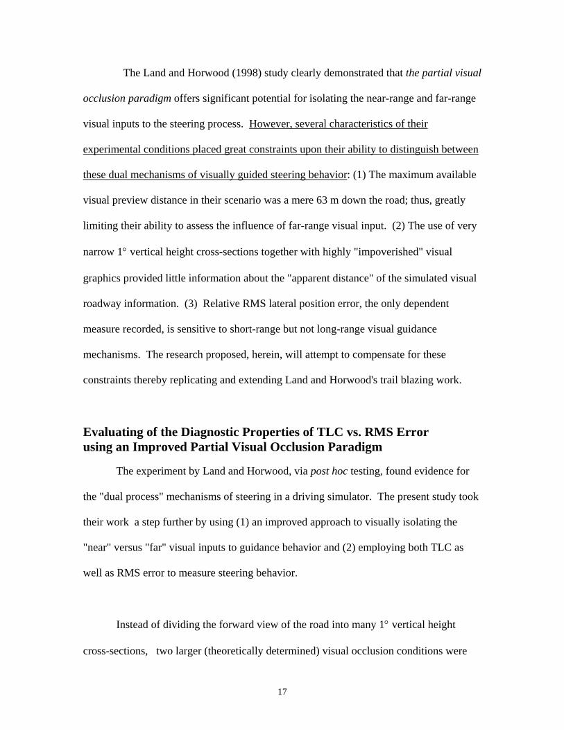
The Land and Horwood (1998) study clearly demonstrated that the partial visual

occlusion paradigm offers significant potential for isolating the near-range and far-range

visual inputs to the steering process. However, several characteristics of their

experimental conditions placed great constraints upon their ability to distinguish between

these dual mechanisms of visually guided steering behavior: (1) The maximum available

visual preview distance in their scenario was a mere 63 m down the road; thus, greatly

limiting their ability to assess the influence of far-range visual input. (2) The use of very

narrow 1° vertical height cross-sections together with highly "impoverished" visual

graphics provided little information about the "apparent distance" of the simulated visual

roadway information. (3) Relative RMS lateral position error, the only dependent

measure recorded, is sensitive to short-range but not long-range visual guidance

mechanisms. The research proposed, herein, will attempt to compensate for these

constraints thereby replicating and extending Land and Horwood's trail blazing work.

Evaluating of the Diagnostic Properties of TLC vs. RMS Error using an Improved Partial Visual Occlusion Paradigm

The experiment by Land and Horwood, via post hoc testing, found evidence for

the "dual process" mechanisms of steering in a driving simulator. The present study took

their work a step further by using (1) an improved approach to visually isolating the

"near" versus "far" visual inputs to guidance behavior and (2) employing both TLC as

well as RMS error to measure steering behavior.

Instead of dividing the forward view of the road into many 1° vertical height

cross-sections, two larger (theoretically determined) visual occlusion conditions were

17

employed. The first of these, hereafter termed the near-only condition, was implemented

by occluding visual access to the road scene beyond two seconds of preview time. Not

only did this block out the view of the road beyond 2 seconds, but any peripheral

information beyond 2 seconds as well. This manipulation was accomplished by blocking

out the top half of the display monitor used to generate the driving scene. The second

experimental condition, hereafter referred to as the far-only condition, was implemented

by occluding visual access to all information in the road scene affording a preview time

of less than 2 seconds. This was done by blocking out the bottom half of the screen used

to render the simulated driving environment. Finally, a baseline condition (where the

entire forward field of view is available to the driver) was used to assess non-restricted

steering performance. There is a somewhat limited field of view in a simulator since there

are constraints made by the monitor viewing area (45 degrees). However, within these

constraints, the forward path of the roadway typically yielded approximately 8 seconds of

preview time - a spatial and temporal extent much better suited for assessing inputs to the

far-range steering process than the previous study using the partial occlusion paradigm.

It has been demonstrated that RMS lateral error and TLC are both useful methods

of measuring driver steering performance. These two measures appear to be sensitive to

separate and distinct behavioral processes mediating automobile steering. The short-

range (closed-loop) steering system depends upon continuous visual sampling of the

section of roadway out to about 2 seconds in front of the vehicle (since RMS steering

error declines as preview time is increased and reaches asymptotic levels of performance

at approximately 2 seconds). Hence, RMS error appears to be insensitive to the long-

18

range visual inputs to the steering process. Because of this one can conclude that

automobile driving research done using only RMS error measurements might not be

capturing the complete story regarding steering performance. It is hypothesized, herein,

that RMS error is an adequate measure of the short-range steering process and that TLC

is better suited for the measurement of the long-range steering process. A test of these

hypotheses would be provided by comparing baseline measures of TLC and RMS error

performance to those obtained under the near-only and far-only partial visual occlusion

conditions described above.

Research Hypothesis 1. Relative to baseline performance, RMS error will remain

unchanged in the near-only condition but increase significantly in the far-only condition.

That is: with only the short-range visual information available to the drivers in the near-

only condition, one would expect RMS error performance to be comparable to that

achieved under baseline conditions (i.e. where the entire forward view was available)

since RMS error is a measure of short-range performance and drivers would have access

to all available short-range information in this condition. However, in the far-only

condition RMS error performance would be expected to suffer since drivers wouldn't

have access to the peripheral edge line information that they use for short-range lane

keeping via compensatory tracking processes.

Research Hypothesis 2. Relative to baseline performance, TLC will remain unchanged in

the far-only condition but decline significantly in the near-only condition. That is: under

the near-only viewing condition TLC performance would be expected to suffer since the

19

drivers would not be afforded the opportunity of seeing the part of the road where they

would theoretically cross the edge line (i.e., information about the future path of the road

needed by the far-range guidance mechanism). In the far-only condition one would

expect driver performance as measured by TLC to be comparable to baseline since TLC

is presumed to be more sensitive to distant visual inputs to the steering process and all

far-range visual information would be available.

Method

Participants. Twenty-one individuals recruited from undergraduate psychology classes at

USD served as participants in this study. Average age of the participants was 24 year

(4 males, 17 females). Mean visual acuity was 20/18 and 20/19 for near and far

distances, respectively.

Apparatus and Materials. The experiment was performed in the fixed-based STISIM

(v.8.0) driving simulator at the University of South Dakota’s Heimstra Human Factors

Laboratories. The simulator is composed of a car seat on a platform in front of a steering

wheel console, a floor mounted accelerator and brake module, and a video display

monitor connected to an IBM compatible computer with the necessary software and

accelerated video graphics capabilities. The near-only and far-only visual cue conditions

discussed earlier were implemented by using cardboard cutouts to occlude the

corresponding sections of the monitor into near and far regions, respectively (see Figure

4). Performance data were collected in real-time using the existing STISIM software.

20

Far-range

Near-range

true horizon

Figure 4. Schematic representation of simulated driving scene showing border between the near-only and far-only occlusion regions.

Procedure. Participants drove on a simulated 2-lane road with alternating straight and

curved sections. The participants were seated in front of the display monitor with the

controls in front of them, as they would in a real automobile. When a trial began the

participant was presented with a 2-lane road with a broken yellow center dividing line.

The participants then drove the simulated vehicle along the pre-designed roadway while

maintaining their proper lane position and speed to the best of their abilities.

On each trial there was a series of 10 curves alternated with straight sections of

road (see Table 1). The curves varied in length and radius. However, each trial consisted

21

of curves of the same radii and straight sections of road that appeared in the other trials,

but in different random orders. For example, the first curve in the beginning trial may

have involved a turn to the left with a radius of 1000 ft. In each of the following trials

there was also a left curve with a radius of 1000 ft but it was not the first curve in the

subsequent trials owing to the randomization procedure.

Radius (ft) Direction

1000 Left 1500 Left 2000 Left 2500 Left 3000 Left 1000 Right 1500 Right 2000 Right 2500 Right 3000 Right

Table 1. Curves used in constructing each of the simulated roadway circuits.

The participants began with a practice trial. This served to familiarize the

participants with the simulator. The practice trial was followed by three experimental

trials: namely, the baseline, near-only and far-only conditions. The order of presentation

for these experimental trials was randomized.

In the baseline trial condition the screen was completely visible with the full

range of near and far visual information available to the drivers. In the near-only

condition visual information with a preview time greater than 2 seconds was occluded.

As such, only the visual area extending out to 176 feet in front of the car remained visible

22

to the driver (assuming a fixed vehicle speed of 60 MPH). In the far-only condition,

however, visual information with a preview time of 2 seconds or less was occluded.

The participants were instructed to stay in the right lane. Participants were further

instructed to maintain a constant predetermined speed (fixed at the maximum speed of

60 MPH by the STISIM software). There was no other traffic on the roadway. Data

regarding longitudinal velocity, lateral lane position with respect to the dividing line,

vehicle heading, current roadway curvature, and heading angle error with respect to the

dividing line were collected via the STISIM software for analysis.

Results

RMS Analysis

Data were collected on 21 participants using the STISIM driving simulator. Each

of the participants negotiated the simulated course in the baseline, near-only, and far-only

viewing conditions. Analysis of the RMS error data was performed using a (3)view x

(2)segment x (2)direction x (4)radius repeated measures ANOVA. In this ANOVA view

describes the previously mentioned near-only, far-only, and baseline viewing conditions,

segment was the average of the straight section of road prior to entering a curve or the

average of the curve data, direction describes whether the curve was to the left or to the

right, and radius was the severity of the curve. Technical limitations of the simulator’s

data recording capabilities necessitated the removal of the 6666 foot radius curves from

23

the RMS error data analysis. As a result, only 4 curve radii were analyzed, those being

3333, 4000, 5000, and 10000 feet.

Corrections for violations of the sphericity assumption (i.e., homogeneity of

covariance) were done using the Huynh-Feldt correction, built into the SPSS analysis

package. Huynh-Feldt was chosen over the Greenhouse-Geisser correction, also built into

the SPSS package due to the overly conservative nature of the Greenhouse-Geisser

correction (Keppel,1973; p.446).

Table 2.

Summary of (3) View by (2) Segment by (2) Direction by (4) Radius ANOVA performed upon the RMS steering error data.

segment direction radius

view x direction

view x segment x direction

segment x radius

direction x radius

segment x direction x radius

df F-test P level view 2,40 49.19 0.000

1,20 16.79 0.0011,20 0.003 0.9573,60 38.83 0.000

view x segment 2,40 12.65 0.0002,40 0.668 0.482

segment x direction 1,20 12.16 0.0022,40 1.56 0.227

view x radius 6,120 4.39 0.0013,60 5.78 0.002

view x segment x radius 6,120 0.929 0.4773,60 0.249 0.862

view x direction x radius 6,120 1.5 0.1923,60 1.94 0.132

view x segment x direction x radius 6,120 1.2 0.311

Table 2 shows the results of the ANOVA. Significant main effects (alpha = 0.05)

were shown for view, segment, and radius, as well as significant two-way interactions for

view by segment, view by radius, segment by radius, and segment by direction.

24

View

00.20.40.60.8

1

Baseline Near Far

Viewing Condition

RM

S er

ror

Figure 5. RMS steering error as a function of experimental viewing condition.

Figure 5 depicts the significant main effect of viewing condition on RMS error.

Post hoc comparisons revealed that the far viewing condition was associated with

significantly greater RMS error than both the baseline ( F(1,20) = 45.3, p < .000 ) and

near-only viewing conditions ( F(1,20) = 78.3, p < 0.000 ). The comparison of the near-

only versus baseline conditions yielded a marginally significant difference

( F(1,20) = 4.38, p < 0.49 ). This pattern of results supports the experimental hypothesis

that drivers use visual information from the near region of the road to support lane

keeping and that changes in RMS error reflect the level of functioning within this “near”

visual process.

25

View x Segment Interaction

00.20.40.60.8

1

approach curve

Road Segment

RM

S er

ror

farbaselinenear

Figure 6. RMS steering error as a function of Viewing Condition and Road Segemnt.

Interpretation of the main effect of viewing condition (see Figure 5) was qualified

by a significant two-way interaction between the road segment (approach vs. curve) and

curve direction variables (left vs. right). Examination of Figure 6 reveals that RMS error

under the near viewing condition never exceeded those observed in the baseline

condition. However, RMS error in the far viewing condition significantly exceeded

baseline in both the approach ( F(1,20)= 51.54, p< .000 ) and the curved roadway

segments ( F(1,20)= 16.99, p<.001 ). It should be noted that the increase in RMS error

associated with the transition from the straight line approach to the curved roadway

section is absent in the far viewing condition ( F(1,20)= .439, p<.906 ).

26

View x Radius Interaction

0.30.40.50.60.70.80.9

11.1

0.00005 0.0001 0.00015 0.0002 0.00025 0.0003

Radius (1/Ft)

RM

S er

ror

baselinenearfar

Figure 7. RMS steering error as a function of Viewing Condition and Curve Radius.

RMS error across viewing conditions also varied as a function of the degree of

roadway curvature (Figure 7) with RMS in the far viewing condition significantly higher

than the near and baseline conditions for all curve radii (p < 0.01). This difference was

especially apparent in the increase between the 10000 and 5000 feet radius curves.

Segment x Radius

0.30.40.50.60.70.80.9

0.00005 0.0001 0.00015 0.0002 0.00025 0.0003

Radius (1/Ft)

RM

S er

ror

ApproachCurve

Figure 8. RMS steering error as a function of Road Segment and Curve Radius.

27

Although not directly related to the experimental hypotheses under investigation,

two additional significant interactions were observed. The nature of the road segment x

radius interaction is depicted in Figure 8. Here we see that RMS error differences

observed across the approach and curve conditions tends to increase with the magnitude

of road curvature. This difference is relatively small for curve radii of 10000 and 5000

feet but significantly greater at curve radii of 4000 ( F(1,20)= 18.44, p<.000 ) and 3333

feet ( F(1,20)= 15.95, p<.001 ).

Segment x Direction

00.20.4

0.60.8

Approach Curve

Road Segment

RM

S er

ror

LeftRight

Figure 9. RMS steering error as a function of Road Segment and Curve Direction.

Finally, the segment x direction of curvature factors were also found to yield a

significant interaction effect (see Table 2). The depiction of this interaction in Figure 9

reveals that the increase in RMS error when transitioning from the straight-line approach

into the curved road segment tended to be slightly greater in the case of right curves.

28

TLC Analysis

Time-to-line-crossing (TLC) data were collected on the same 21 participants

under the same viewing conditions (baseline, near-only, and far-only) considered for the

RMS error analyses . The STISIM version 8 software used to conduct this study did not

directly generate time-to-line-crossing measurements. These measures were computed

off-line using software that modeled the future path of the vehicle based upon a

continuous data log of vehicle state variables (such as heading, lane position, velocity,

acceleration, etc.). Unfortunately, the software used to generate the TLC measure

produced “unstable” results for curves involving right turns used in this study. As a

result, the analysis of TLC data was limited to left curves only. Also of note, the data

collection difficultly that necessitated the removal of the 6666 foot radius curves in the

RMS analysis was not present in the TLC data. Therefore, data from all 5 curve radii

were included in the TLC analysis.

Results of a (3) viewing condition x (5) curve radius repeated measures ANOVA

for the TLC data collected while driving in left curve roadway segments are detailed in

Table 3. Significant results were found for the main effects of viewing condition and

curve radius in the TLC analysis.

Table 3.

Summary of (3) Viewing Condition by (2) Segment by (5) Radius ANOVA performed upon the time-to-line-crossing (TLC) data.

Effect df F PViewing Condition 2,40 3.83 0.030 Radius 4,68 393.2 0.000 View x Radius 2,46 2.94 0.055

29

Although the main effect of viewing condition was statistically significant, the

pattern of TLC differences observed across viewing conditions was inconsistent with the

predictions of the main experimental hypothesis (see Figure 10).

TLC View

0

5

10

15

20

Baseline Near Far

Viewing Condition

TLC

(sec

onds

)

Figure 10. TLC as a function of Viewing Condition.

Rather than demonstrating the expected TLC level comparable to baseline for the far-

only viewing condition, the actual observed value was significantly lower than baseline

( F(1,20)= 6.95, p<.016 ). Also inconsistent with the hypothesis was the failure to observe

significant reductions in average TLC for the near-only viewing condition relative to

baseline ( F(1,20)=2.42, p<.135 ).

30

TLC Radii

05

1015202530

10000 6666 5000 4000 3333

Radius (feet)

TLC

(sec

onds

)

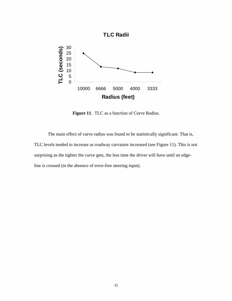
Figure 11. TLC as a function of Curve Radius.

The main effect of curve radius was found to be statistically significant. That is,

TLC levels tended to increase as roadway curvature increased (see Figure 11). This is not

surprising as the tighter the curve gets, the less time the driver will have until an edge-

line is crossed (in the absence of error-free steering input).

31

Discussion

There are a number of possible explanations for the failure to obtain support for

the hypothesis that the TLC measure would be differentially sensitive to the “far” visual

process in automobile steering . In this document we have described how TLC could be

conceptualized as a proxy for the far range process drivers use to prepare for upcoming

maneuvers. However, the obtained pattern of results strongly suggests that it’s quite

unlikely that the status of such a highly complex, cognitively-based anticipation system

can be captured adequately by a single performance parameter (i.e., time-to-line-

crossing).

A second possible explanation for the failure to observe the predicted outcome for

the TLC data is that the low resolution of the simulator may not have been sufficient to

render critical visual information in the far viewing area (over 2 seconds away). The

graphical display of the STISIM simulator was rendered at the very limited resolution of

640 (horizontal) x 480 (vertical) x 256 (colors). Given this impoverished level of spatial

resolution, upcoming curves often resembled a single line leading off to the left or right,

rather than a road with an actual width and other discernible properties. This particular

version of the simulator also does not allow for elevation changes in the scene which

eliminates the possibility of adding hills and dips - rendering a view that is relatively

featureless. Couple this with the low display resolution and it becomes difficult to

accurately judge the distance to an upcoming curve as well as the severity of the curve.

Another possibility deals with the design of the test circuits themselves. In this

study the participants were instructed to simply put the accelerator pedal to the floor and

leave it there. Since the simulator was preprogrammed to allow a top speed of 60 MPH

32

this procedure provided the equivalent of an “automatic cruise control”. By setting this

condition it became necessary to design a road scenario that would actually be “drivable”

by participants obeying the 60 MPH instructions. In order to accomplish this the radii of

the curves had to be minimized, otherwise the vehicle would stand a great chance of

leaving the road under the near-only viewing condition resulting in a crash, which would

then reposition the vehicle in the center of the right lane and reset the vehicle speed to 0

(resulting in an undefined driving event and a complete loss of data for the road

segment). By designing the curves to a maximum curvature standard it had the desired

effect of minimizing crashes but it also may have had the undesired effect of making the

curves highly “recoverable”. That is, drivers had sufficient time to turn the wheel when

they entered a curve -- even without being able to see it coming -- to avoid leaving the

road surface. This highly forgiving circumstance could have affected their TLC

performance. It’s possible that TLC might paint a different picture under more severe

driving conditions. In fact, most previous applications of the TLC measure have

employed relatively severe roadway geometies.

The RMS error data did provide support for the idea that the near view is where

the driver’s glean information pertaining to maintaining vehicle roadway position. Our

ANOVA results demonstrated how RMS error increased dramatically in the far-only

viewing condition (figure 6) and actually decreased in the near-only viewing condition.

This finding suggests a “recruitment of effort” effect. That is, when the information

beyond 2 seconds is removed drivers were forced to become more vigilant in their lane

position monitoring and, as a result, RMS error actually improved a bit under this

condition.

33

The loss of the near preview area was especially detrimental to the roadway

segments with the greatest degree of curvature (as Figure 7 shows). RMS error was also

greater, as expected, in curves than in the straightaway sections preceding the curves

under the near-only and baseline conditions as shown in Figure 5. One curious discovery

was a direction difference in the curves demonstrating that RMS error was different

between curves to the right and curves to the left (Figure 8). This might be due to the fact

that there was no oncoming traffic in the study and in a right turn the drivers would have

more time to react and more space to work with before reaching the edge of the road. Our

participants apparently took maximum advantage of this opportunity.

Our modification of Land’s original occlusion paradigm (one degree horizontal

strips of visible roadway) yielded the expected results in the case of RMS error data.

Given the improved ecological validity of the near/far approach used in the present study,

this method could be recommended for future applications. Blocking the drivers view out

beyond 2 seconds is a phenomenon that does occur out in real world driving, such as in

fog, at night, or in heavy rain/snow.

Despite the disappointment with the TLC results, we plan to study the feasibility

of repeating this study in a more advanced simulator or possibly on a closed test track.

Repeating this study on a track would likely yield the best results given the inherent

weaknesses of fixed-based driving simulators; namely, their limitations in the ability to

render dynamic visual-spatial details.

34

References

Donges,E. (1978). A two-level model of driver steering behavior. Human Factors,

20(6), 691-707.

European Communities. (1999). COST 331: Requirements for horizontal road

marking. Luxembourg: Office for official publications of the European Communities.

Godthelp, H., Milgram, P., & Blaauw, G.J. (1984). The development of a time-

related measure to describe driving strategy. Human Factors, 26(3), 257-268.

Godthelp, H.(1986). Vehicle control during curve driving. Human Factors, 28(2),

211-221.

Gordon, D. (1966). Experimental isolation of drivers’ visual input. Public Roads,

33(12), 266-273.

Herrin, G.D., & Neuhardt, J.B. (1974). An empirical model for automobile driver

horizontal curve negotiation. Human Factors, 16(2), 129-133.

Keppel, G. (1973). Design and analysis: A researchers handbook. Englewood

Cliffs, NJ. Prentice-Hall.

Land, M.F., & Lee, D.N. (1994). Where we look when we steer. Nature, 369,

742-744.

Land, M.F., & Horwood, J. (1995). Which parts of the road guide steering?

Nature, 377, 339-340.

Land, M.F., & Horwood, J. (1998). How speed affects the way visual information

is used in steering. Vision in Vehicles-VI, 43-50.

McLean, J.R., & Hoffman, E.R. (1973). The effects of restricted preview on

driver steering control and performance. Human Factors, 15(4), 421-430.

35

Summala, H., Nieminen, T., & Punto, M. (1996). Maintaining lane position with

peripheral vision during in-vehicle tasks. Human Factors, 38(3), 442-451.

Summala, H. (1998). Forced peripheral vision driving paradigm: Evidence for the

hypothesis that car drivers learn to keep in lane with peripheral vision. Vision in

Vehicles-VI, 51-60.

Van Winsum, W., Godthelp, H., (1996). Speed choice and steering behavior in

curve driving. Human Factors, 38(3), 434-441.

Van Winsum, W., Brookhuis, K.A., & de Waard, D. (2000). A comparison of

different ways to approximate time-to-line crossing(TLC) during car driving. Accident

Analysis and Prevention, 32, 47-56.

36