the effects of infrastructure development and taxation on
TRANSCRIPT

Syracuse University Syracuse University
SURFACE SURFACE
Economics - Dissertations Maxwell School of Citizenship and Public Affairs
5-2012
The Effects of Infrastructure Development and Taxation on The Effects of Infrastructure Development and Taxation on
Current and Future Earnings Current and Future Earnings
Mukta Mukherjee Syracuse University
Follow this and additional works at: https://surface.syr.edu/ecn_etd
Part of the Economics Commons
Recommended Citation Recommended Citation Mukherjee, Mukta, "The Effects of Infrastructure Development and Taxation on Current and Future Earnings" (2012). Economics - Dissertations. 92. https://surface.syr.edu/ecn_etd/92
This Dissertation is brought to you for free and open access by the Maxwell School of Citizenship and Public Affairs at SURFACE. It has been accepted for inclusion in Economics - Dissertations by an authorized administrator of SURFACE. For more information, please contact [email protected].

ABSTRACT
This dissertation is a collection of three essays, each of which studies a policy in
India that provides a unique circumstance a¤ecting directly or indirectly earnings.
The purpose of this work is to analyze how taxation and infrastructure development
a¤ects the current and future earnings using these policies.
In the �rst essay, I use a national infrastructure development program initiated in
India in 2001 to construct new all-season roads (roads that can be used in all-weather
especially monsoons) in villages that previously had only had dry-season roads (roads
that are di¢ cult to use in monsoons). In the second, I use a new tax on fringe bene�ts
initiated in India in 2005, seeking evidence for the hypothesis that the di¤erence in
higher marginal tax rates on wages, relative to lower rates on fringe bene�ts, induces
a reallocation of the total compensation package toward fringe bene�ts. In the �nal
essay, which uses the same policy as that of �rst I am interested behind the economic
motives of manipulation by the local community to obtain public good road in their
locality.

The Effects of Infrastructure Development and Taxation
on Current and Future Earnings
BY
Mukta Mukherjee
DISSERTATION
Submitted in ful�llment of the requirements for degree of Doctor of Philosophy in
Maxwell School of Citizenship and Public A¤airs.
Syracuse University
May 2012

Copyright c Mukta Mukherjee
All Rights Reserved

To my biggest critic-
My mother
&
A father who is present with me in soul

ACKNOWLEDGMENT
This dissertation is a product of a long journey which when I embarked I did not
knew it will be full of uncertainties. Along the way not only I have developed as a
researcher but became a new person. There were people whose encouraging words
allowed me to sustain this path. Foremost, I would like to thank my advisor Je¤rey
Kubik who taught me the art of thinking out of the box. With his kind nature he
made me comfortable to put forth my stupid questions and translated them into
intelligent ones. I am also thankful to my other committee member Devashish Mitra
who gave me constructive inputs at various points during my work.
A word of sincere thanks to those teachers Abhijit Banerjee, Debabrata Datta,
Indira Rajaraman who saw in me some potentiality when I could see none and kept
their faith in me. I will be ungrateful if I omit to mention Chiwa Kao and Badi Baltagi
for their decision which enabled me to be a part of the Department of Economics of
Syracuse University.
I am especially thankful to my friends in Albany Sohini Sahu, Arindam Mandal
and Siddhartha Chattopadhay whose caring attitude sustained me in mymost di¢ cult
part of the dissertation. I am also grateful to two of my seniors Asha Sundaram and
Fariha Kamal for their help in the initial stage of my dissertation. A word of thanks
to my other beloved friends Oindree, Gitu and Muna, whose faith in my potentiality
cheered me up in many bad days.
I am grateful to god to have a loving brother who provided me encouragement in
times when he was going through great personal worries. Lastly this is a tribute to
two persons- my mother who taught me to take criticism with a positive note and
without whom my world will not be the same; the thoughts of my father who was
iv

present with me in soul that inspired me even in most di¢ cult times.
.
v

Contents
1 Introduction 1
2 Do Better Roads Increase School Enrollment? Evi-
dence from a Unique Road Policy in India 1
2.1 Introduction . . . . . . . . . . . . . . . . . . . . . . . . . . . . . . . . 1
2.2 Background . . . . . . . . . . . . . . . . . . . . . . . . . . . . . . . . 5
2.3 Human Capital Investment with a Travel Cost . . . . . . . . . . . . . 7
2.4 Estimation Strategy and Identi�cation Assumptions . . . . . . . . . . 10
2.5 Data Characteristic: PMGSY, Census Village Directory and NUEPA 14
2.6 E¤ects of Improved Access on School Enrollment . . . . . . . . . . . 16
2.6.1 Basic Results . . . . . . . . . . . . . . . . . . . . . . . . . . . 16
2.6.2 Graphical Analysis . . . . . . . . . . . . . . . . . . . . . . . . 16
2.6.3 Empirical Analysis . . . . . . . . . . . . . . . . . . . . . . . . 18
2.7 Impacts of New Roads on Students�Enrollment across Di¤erent Age
Cohorts . . . . . . . . . . . . . . . . . . . . . . . . . . . . . . . . . . 21
2.8 Impacts of New Roads on Students�Enrollment across Di¤erent Social
Background . . . . . . . . . . . . . . . . . . . . . . . . . . . . . . . . 23
2.9 Robustness Check: Placebo Test . . . . . . . . . . . . . . . . . . . . . 25
2.10 Conclusion . . . . . . . . . . . . . . . . . . . . . . . . . . . . . . . . . 26
2.11 Tables and Figures . . . . . . . . . . . . . . . . . . . . . . . . . . . . 28
3 The E¤ect of Fringe Bene�t Tax on Wages: Evidence
from India 39
3.1 Introduction . . . . . . . . . . . . . . . . . . . . . . . . . . . . . . . . 39
vi

3.2 Implementation and Abolishment of the Fringe Bene�ts Tax (FBT) . 42
3.3 Modeling Preferences of Employees for Compensation Components . . 44
3.4 Identi�cation technique . . . . . . . . . . . . . . . . . . . . . . . . . . 49
3.5 Data Characteristic: CMIE and ASI . . . . . . . . . . . . . . . . . . 52
3.6 Result . . . . . . . . . . . . . . . . . . . . . . . . . . . . . . . . . . . 55
3.6.1 Basic Results . . . . . . . . . . . . . . . . . . . . . . . . . . . 55
3.6.2 Heterogeneous E¤ect of Fringe Bene�ts Tax . . . . . . . . . . 57
3.6.3 Hierarchy in the Provision of Productive Fringes . . . . . . . . 60
3.6.4 Robustness Check: Placebo Test . . . . . . . . . . . . . . . . . 62
3.7 Conclusion . . . . . . . . . . . . . . . . . . . . . . . . . . . . . . . . . 63
3.8 Tables and Figures . . . . . . . . . . . . . . . . . . . . . . . . . . . . 66
4 Economic Incentives of Manipulation for Public Good:
Evidence from an Unique Road Policy in India 76
4.1 Introduction . . . . . . . . . . . . . . . . . . . . . . . . . . . . . . . . 76
4.2 Background . . . . . . . . . . . . . . . . . . . . . . . . . . . . . . . . 79
4.3 Economics of Manipulation to obtain Road . . . . . . . . . . . . . . . 81
4.4 Estimation Strategy . . . . . . . . . . . . . . . . . . . . . . . . . . . 82
4.5 Data . . . . . . . . . . . . . . . . . . . . . . . . . . . . . . . . . . . . 84
4.5.1 Manipulation of Road Thresholds . . . . . . . . . . . . . . . . 84
4.5.2 Political Alignment . . . . . . . . . . . . . . . . . . . . . . . . 86
4.5.3 Roads Complementing other Facilities in Districts . . . . . . . 88
4.5.4 Mapping Parlimentary Constituencies into District Data . . . 90
4.6 Incentives to Manipulate to obtain Road . . . . . . . . . . . . . . . . 90
4.6.1 Basic Results . . . . . . . . . . . . . . . . . . . . . . . . . . . 90
vii

Empirical Analysis . . . . . . . . . . . . . . . . . . . . . . . . 91
Graphical Analysis . . . . . . . . . . . . . . . . . . . . . . . . 93
4.6.2 Factors leading to be Politically Sensitive to a Particular Group 94
4.7 Conclusion . . . . . . . . . . . . . . . . . . . . . . . . . . . . . . . . . 95
4.8 Tables and Figures . . . . . . . . . . . . . . . . . . . . . . . . . . . . 97
5 Appendix 108
5.1 Appendix to Section 2 . . . . . . . . . . . . . . . . . . . . . . . . . . 108
5.1.1 Data Appendix . . . . . . . . . . . . . . . . . . . . . . . . . . 108
5.2 Appendix to Section 3 . . . . . . . . . . . . . . . . . . . . . . . . . . 112
5.2.1 Calculating the E¤ective Fringe Bene�t Tax-Rate of Firms . . 112
5.2.2 Data Appendix . . . . . . . . . . . . . . . . . . . . . . . . . . 114
5.3 Appendix to Section 4 . . . . . . . . . . . . . . . . . . . . . . . . . . 116
5.3.1 Data Appendix . . . . . . . . . . . . . . . . . . . . . . . . . . 116
6 References 120
7 Vitae 127
viii

List of Illustrative Materials
Essay1
Figure 1a Schooling Increases with Better Connectivity
Figure 1b Schooling Remains Same with Better Connectivity
Figure 1c Schooling Decreases with Better Connectivity
Figure 2 McCrary(2008) Test for Manipulation at 500 cuto¤
Figure 3 New Roads Construction between Eligible vs Ineligible Villages
Figure 4 Total Enrollment (All) between Eligible vs Ineligible Villages
Figure 5 Trends in Total Enrollment across years for Eligible vs Ineligible
Villages
Figure 6 Placebo Test (Top Panel-Left Median),(Bottom Panel-Right Me-
dian)
Table 1 Descreptive Statistics (Full Sample)
Table 2 Tests of the Identifying Assumption of the RD Analysis (Full Sam-
ple)
Table 3 First Stage Results for Discontinuity Samples
Table 4 2SLS Estimates for All grades in 2009 (Full Sample)
Table 5 Regression Discontinuity for Discontinuity Samples
Table 6 Age -wise E¤ect of New Road on Total Enrollment (Full Sample)
ix

Table 7 E¤ect of New Road on Total Enrollment by Caste (Full Sample)
Essay 2
Figure 1 Trends of Fringes and Wages over Time for All Industries
Figure 2 Revenue Collection Trends of Fringe Bene�t Tax in India
Figure 3 Trends in Average Wages (All Employees) across Concession vs
Non-Concession Sectors
Figure 4 Trends in Average Wages (Managers) across Concession vs Non-
Concession Sectors
Figure 5 Trends in Log (Average) Executive Wages across Concession vs
Non-Concession Sectors
Table 1 FBT Heads and Valuation Base Rate
Table 2 E¤ective Tax Rate of FBT
Table 3 Descriptive Statistics of Selected Variables at Industry-level (with
ASI)
Table 4 Descriptive Statistics of Selected Variables at Firm-level (with
CMIE)
Table 5 Job-wise Variation in E¤ects of FBT on Employees�Wages in an
Industry (with ASI)
Table 6 Heterogeneous E¤ects of Fringe Bene�ts on Executive Wages in a
Firm (with CMIE)
x

Table 7 Elasticity of FBT on Employees�Wages
Table 8 Untangling True E¤ects from Spurious Correlation of FBT on
Wages (with ASI)
Table 9 Untangling True E¤ects from Spurious Correlation of FBT on
Wages (with CMIE)
Essay 3
Figure 1 McCrary test for Manipulation around 250 Threshold (Panel A-
Manipulated States, Panel B-Un-manipulated States)
Figure 2 McCrary test for Manipulation around 500 Threshold (Panel A-
Manipulated States, Panel B-Unmanipulated States)
Figure 3 Figure3-Spatial Pattern of Manipulation Index at Threshold 250
across Sample Districts
Figure 4 Figure4-Spatial Pattern of Manipulation Index at Threshold 500
across Sample Districts
Figure 5 Figure5-Spatial Pattern of Incumbent�s Political Alignment across
Sample Districts
Figure 6a Agricultural land Distribution among eligible and ineligible villages
in Manipulated States at Threshold 250
Figure 6b Agricultural land Distribution among eligible and ineligible villages
in Un-Manipulated States at Threshold 250
Figure 7a Agricultural land Distribution among eligible and ineligible villages
in Manipulated States at Threshold 500
Figure 7b Agricultural land Distribution among eligible and ineligible villages
in Un-Manipulated States at Threshold 500
Table 1 Correlation between Formal McCrary Test and Informal Manipu-
lation Indexxi

Table 2 Descreptive Statistics
Table 3 Di¤erent Incentives to Manipulate Road at Threshold 250
Table 4 Di¤erent Incentives to Manipulate Road at Threshold 500
xii

1 Introduction
India is a country where one would �nd individuals with wide variation in earn-
ing�s capacity. Whereas in one hand exists CEO�s of multinational draws prince�s
ransom, on the other hand there are people living in villages who can barely meet
their necessity. Therefore, the factors that can a¤ect the earnings of an individual
especially in a developing country context are an important area of study. This dis-
sertation is a collection of three essays, each of which studies a policy in India that
provides a unique circumstance a¤ecting directly or indirectly earnings of individuals
drawn from di¤erent stratum of the society. The purpose of this work is to analyze
how taxation and infrastructure development a¤ects the current and future earnings
using these policies.
In the �rst essay, I use a national infrastructure development program initiated
in India in 2001 to construct new all-season roads (roads that can be used in all-
weather especially monsoons) in villages that previously had only had dry-season
roads (roads that are di¢ cult to use in monsoons). The eligibility rule that was
used for undertaking construction of new all-season roads in these villages was that
a minimum population of 500 had to be bene�t from this road. This eligibility
rule induced a nonlinear relationship between the population and the number of
new all season roads in the villages of India today. In order to control for factors
like communities�collective action ability that simultaneously determine the timing
of completion of roads and students� enrollment in the schools, I instrument new
roads with the population eligibility criteria. Exploiting the exogenous nature of the
1

program eligibility criteria I compare students�enrollment in schools between villages
on either side of the population cuto¤. The most conservative estimates show that an
improved access to school by better roads increases school enrollment by 22 percent
in 2009. I �nd no spurious e¤ects in 2002 when the same villages did not have a
road. The e¤ect of better access to roads on students�enrollment is heterogeneous
depending on the age cohort and the caste (social background) to which they belong.
In the second, I use a new tax on fringe bene�ts initiated in India in 2005, seek-
ing evidence for the hypothesis that the di¤erence in higher marginal tax rates on
wages, relative to lower rates on fringe bene�ts, induces a reallocation of the total
compensation package toward fringe bene�ts. Firm-level panel data on employee to-
tal compensation and wages across all industries is used to link their marginal tax
rate on fringe bene�ts and choice of compensation. The key �nding is that a tax on
fringe bene�ts only a¤ects the wage allocation of highly paid employees relative to
employees lower on the pay scale. Using the most conservative estimate, the research
shows that a doubling of the fringe-tax increases wages by one percent. Further, I
�nd that this reallocation is more evident for fringe bene�ts, such as private pensions
(private-fringe bene�t) relative to travel and lodging expenditures which can enhance
a �rm�s productivity (productive-fringe bene�t).
In the �nal essay, which uses the same policy as that of �rst I am interested
behind the economic motives of manipulation by the local community to obtain public
good. I use data from a universal scheme initiated in India in 2001 to build new all-
season roads in villages of India to understand how the various eligibility thresholds
for the road policy has been manipulated at the district level during the period of
implementation. Results show that the higher economic returns drive the desire to
2

obtain a road in the locality. The better o¤ sections of the economy are driven by
the complementary role between the roads and other facilities, whereas the poorer
sections try to substitute with a poor provision of other public goods. Further, I �nd
the politicians in a particular state are substituting the better-o¤voters with the poor
voters with a motive of maintaining high representation in the government.
3

2 Do Better Roads Increase School Enrollment? Evidence
from a Unique Road Policy in India
2.1 Introduction
Physical distance to school is cited as a major barrier to participation for rural
children in India (UNICEF, 2006; Ward, 2007). Similarly, in many other developing
countries schools are not easily accessible1, thus social scientists and policy makers
are interested considerably in whether better access to schools increases students�
enrollment (Du�o, 2001; Filmer, 2007; Handa, 2002). For example, in India, on
average in most villages primary schools are one km away, middle schools are at three
km away and secondary and higher secondary are �ve km away from the village center
(Census, 2001; Ward, 2007). A considerable travel time is involved in accessing these
schools. This time lost in travelling cannot be used either for productive activities or
for leisure. It is just the additional cost that has to be borne to acquire education and
is not used in actual learning. In many instances, the distances have to be covered
on foot which leads to physical discomfort especially in hot summers and monsoons.
The time lost is a major implicit cost in schooling decision.
Irrespective of this considerable interest in consequences of better access for school
enrollment, measuring casual e¤ects of access to school on schools�enrollment has
proved to be very di¢ cult. One of the common measures used is the new school
availability in the locality (Du�o, 2001; Foster and Rosenweig, 1996; Jalan and Glin-
1The average distance required by a child to travel to reach the nearest primary schools rangesfrom 0.2 km in Bangladesh to 7.5 km in Chad. The distance to the nearest secondary schools rangesfrom 2 km in Bangladesh to 71 km in Mali (Filmer, 2007).
1

skaya, 2003). However, the placement of schools is not random. Usually the new
schools are constructed in localities which previously su¤ered from low enrollment.
This will lead to under estimation of the impact of the bene�ts of an improved access
to schools on enrollment. On the other hand, if families who value schooling move
towards localities with better schooling or schools are constructed in areas where the
people value more education, the impact on enrollment will be over estimated. An-
other measure that has been used in cross-country studies is the average distance to
the nearest primary or secondary schools or travel time on enrollment (Filmer, 2007;
Bommier and Lambert, 2000; Handa, 2002). A robust pattern observed in most
of these studies (Du�o, 2001; Jalan and Glinskaya, 2003; Filmer, 2007) is that the
impact is highest for those who are interiorly located; usually these are the poorer
sections.
In this study I use the regression discontinuity technique to surmount the fun-
damental problem of identi�cation that the previous literature su¤ered from. This
study uses a new measure for better access to schools by exploiting the provision of
new all-season roads (roads that can be used in all weather especially monsoons) as a
part of a national infrastructural program which was initiated in 2001 in India. The
provision of new all-season roads (roads that can be used in all weather especially
monsoons) in villages which previously only had dry-season roads (roads that are dif-
�cult to use in monsoons) were done on the basis of a population eligibility criteria.
This rule generates a potentially exogenous source of variation in the provision of new
all-season roads which can be used to estimate the e¤ects of better access to schools
on the students�enrollment in rural India.
The importance of the population criteria rule in this study is that it can be used to
2

determine the provision of new all-season roads in villages on the basis of their villages�
population as in 2001. The implementation of the policy is as follows. According to
the population criteria rule, there is no provision of all-season roads in villages when
the population recorded is between 100 and 499, but when the population recorded is
more than 500 then there is a sharp increase in the provision of all-season roads. In
this study, villages with more than 500 populations as recorded in 2001 have a twenty
�ve higher probability of being provided with a new all-season road. This study uses
a novel dataset compiled from administrartive reports linking school enrollment at
the village level to the number of new all-season roads.
Usually, in India the provision of public goods is simultaneously determined by
many other factors. According to Banerjee, Iyer and Somanathan (2008) the com-
munities�collective action ability is a major factor determining both the provision of
public goods like roads and facilities in schools, a¤ecting students�enrollment in India.
In this study, I use the population rule to construct instrumental variable estimates of
better roads e¤ects. The most conservative estimates show that an improved access
to school by better roads increases school enrollment by 22 percent in 2009. Further,
the e¤ect of better access to roads on students�enrollment is heterogeneous depending
on the age cohort and social background to which they belong. The development of
roads brings forth both intended and unintended e¤ects on students�enrollment in
school. Whereas for the younger students�participation rate in school increases, for
the older students�participation rate in school decreases. The participation response
of enrollment to a development of better roads is much higher for students from higher
caste (students belonging to the higher social hierarchy scale) compared to those from
backward caste (students belonging to the lower social hierarchy scale).
3

A possible explanation of the heterogeneous e¤ects of roads on students on the
basis of their age and social background is the following. The �rst phenomena can be
explained in a child economy context with outside job opportunities. In comparison to
the younger age cohort the higher age cohort students are physically able to reap the
bene�t of better job opportunities that a better connectivity brings forth; therefore
their incentive to participate in school decreases with a development of a road. A
possible explanation of the second phenomena is that the backward caste students
in one hand bene�ts most from the development of better roads as they stay in
the vicinity of the village, but in the other hand these students reaps less from an
investment in schooling as the social restrictions they face constraints their future
wage earnings.
The contribution of this paper is manifold. This study provides new insight into
the question of whether students�enrollment increases with better access to school
which has always interested economist and policy makers simultaneously. The study
also contributes to a scanty body of literature on the measurement of economic ben-
e�ts that comes with a better connectivity (Jacoby, 1998; Jacoby, 2008). Usually
the bene�ts of an improved connectivity are calculated on the basis of hypothetical
projects in countries like Nepal and Madagascar due to the lack of real instances.
This unique road scheme allows study of the economic bene�ts from a wide scale real
construction of roads. This paper overcomes limitations in the other past studies as
it uses a novel dataset constructed from the administrative reports on eligible villages
and their new roads completion information.
The remainder of the paper proceeds as follows: Section 2 lays down the details of
the national infrastructure road development program introduced in India. Section
4

3 provides a brief theoretical framework of human capital investment and time lost
in travelling. Section 4 discusses the identi�cation technique and the data used for
the analysis. Section 5 explores the empirical �ndings, with some robustness checks.
Section 6 summarizes our �ndings and some limitations of the study.
2.2 Background
In India, roads form the life-line of villages as the access to schools, market and
health centers is dependent on it. According to Bell (2010) the bene�ts of better
roads in villages is manifold. First, as consumers they enjoy a reduced prices and as
producers they can negotiate for higher price for their marketable surplus. Second, as
students they can access schools located outside village. Finally, with a better access
to medical amenities and crucial drugs not only can their health condition improve
but it actually can make a di¤erence between life and death in several scenarios.
However, forty percent of all villages in 2000 were still unconnected by roads.
In 2001,2 a national infrastructure development program PMGSY was initiated
to ful�ll the gap of roads in villages. The primary objective of this policy was to
provide all-season roads to hamlets3 that previously did not have any all-season roads
within 0.5 km4. A secondary objective of this scheme was to upgrade the already
existing all-weather roads based on the roads�deterioration. This gave emphasis to
more populated areas, however only 20 percent of the funds were to be allocated
towards this goal and the other 80 percent of the funds would be allocated towards
2The policy was declared on 25th December, 2000.3A hamlet is a cluster of population, living in an area, the location of which does not change over
time.4The eligibility condition for new all weather roads for hilly states (North-East, Sikkim, Himachal
Pradesh, Jammu & Kashmir, Uttaranchal), desert areas (districts, blocks eligible for Desert Devel-opment Projects) and Schedule 5 areas (constitution prescribed districts, block and villages withhigh populations of schedule castes and tribes) is that within a radius of 1.5km no all-weather roadsexist and the minimum bene�ted populations has to be 250 at least.
5

the ful�llment of the primary objective.
The provision of new all-season roads followed an eligibility rule. The eligi-
bility rule for a new all-season road (NR) linking several unconnected5 hamlets
(h1; h2; ::::::::::hn) whose populations as recorded in Census 2001 (p1; p2; ::::::::::pn)
that would be considered for construction is given in equation (2.1). Equation (2.1)
captures the fact that the PMGSY rule allows the unconnected hamlets with a popu-
lation greater than 500 to receive new roads but hamlets eligible by virtue of distance
with a population of 100-499 do not receive a new road. The discontinuity created by
the 500 population threshold will be used as an identi�cation strategy in this study.
NR = 1 if max (p1; p2; ::::::::::pn) >= 500 (2.1)
= 0 if max (p1; p2; ::::::::::pn) < 500
The PMGSY was a national policy with an estimated cost of $14 billion (Rs
600 billion) and more emphasis was given to states that had eligible unconnected
hamlets. However, there is a great deal of state-wise variation in the progress of
the construction and completion of new roads, depending on the local government
initiative. In some states the federal grants were a part of a loan sanctioned by the
World Bank (Jharkhand, Rajasthan, Uttar Pradesh, Himachal Pradesh) and Asian
Development Bank (Assam, West Bengal, Orissa, Madhya Pradesh, Chhattisgarh).
In return these states had to meet some conditions for safeguarding local environment
and communities6. However, the eligibility rule for new all-season roads did not vary
5The hamlet would be considered unconnected if it does not have an all-weather road within a0.5km radius.
6The existing standards were appraised and modi�ed to minimize impacts on communities and
6

between the World Bank and ADB sponsored states and other non-sponsored states.
2.3 Human Capital Investment with a Travel Cost
This section presents a simple human capital investment model that informs the
empirical analysis.
Optimal level of Schooling Given that there is no productivity growth, the present
value of life-time earnings of a "representative" individual with s years of education,
evaluated at the age of school entry is
V (s; r) =
nZ0
y(s; �)e�r(s+x)dx� C(s; �); (2.2a)
where fy(s; �)g is based on the estimated statistical earnings and r is the discount
rate. The life-time earnings in (2.2a ) can be expressed as
V (s; r) =fy(s; �)g e�rs (1� e�rn)
r� C(s; �); (2.2b)
The individual maximizes the life-time earnings in (2.2b) w.r.t. choice of schooling
s. The �rst order condition is given by
fys � ryge�rs (1� e�rn)r
� Cs = 0; (2.3)
With an improvement in the state of connectivity the equilibrium choice of school-
ing is (refer Theory Appendix )
ds
d�= � e�rs (1� e�rn) [ys� � ry� ]� rCs�
e�rs (1� e�rn) [yss � rys + ry2]� rCss; (2.4)
environment.
7

In (2.4) the denominator would always be negative to satisfy the second order
condition for maximization. Therefore, the equilibrium choice of schooling would
depend on the numerator. The �rst term [ys� � ry� ] denotes the present value of
net gains from additional schooling after adjusting for forgone earnings. With an
improved state of connectivity there would be two e¤ects operating in the opposite
direction ; (ys� ) the bene�ts from earnings from an additional period of schooling
and ry� the forgone earnings adjusted for the interest rate. With a better access
to the employment opportunities the potential wage earnings y� would also increase,
thus the latter term also increases. Hypothetically, ys� R 0 , but in reality for a
short span of time ys� < 0 can be ruled away. This implies that better connectivity
leads to higher competition and that the returns from schooling decreases. But,
such a scenario would take considerable time even after development in the level of
transport. The second term rCs� denotes the present value of cost of travelling to
school after there is an improvement in connectivity. This term is always negative on
the basis of assumption that travel cost to school decreases with an improvement in
connectivity. The schooling choice of the individual would depend upon which of the
two e¤ects dominate as is given in (2.5)
ds
d�R 0 if [ys� � ry� ] R 0: (2.5)
There are three possible cases depicted in Figure 1, but with each of them, with an
improved state of connectivity the individual can reach a higher iso-wealth curve and
is always better o¤ than in the earlier state. The individual would choose a higher
(lower) schooling level, when the net earnings gained from an additional period of
schooling dominates (is dominated by) the loss of forgone earnings. If the two e¤ects
8

exactly o¤set each other the schooling level will remain unchanged.
Hypothesis 1 In an improved state of connectivity, the lower the outside wage
earnings potential the higher is, the higher the incentive to remain in school. Thus
in an economy with child-labor opportunities increasing with an improved connectiv-
ity, the lower age group who are not physically �t to work have higher incentive to
participate in school than a higher age group who can work (Basu, 1999). This leads
to a following ranking of the schooling choice among di¤erent age groups less than 5
years, 5 to 9 years, 10 to 14 years and more than 147.
ds
d� less than 5yrs>ds
d� 5�9yrs>ds
d� 10�14yrs>ds
d� 15�18yrs: (2.6)
Hypothesis 2 In an economy where there is heterogeneity among sections by eco-
nomical and social background, the bene�ts of an improved connectivity on di¤erent
sections�students is ambiguous. In India, the schools are usually spatially clustered in
the high caste8 dominant areas and the low castes reside outside the villages. Thus, a
village school would still be a considerable walking distance for these students. There-
fore, the lower caste students would reap the bene�t of an improved connectivity more
than the higher caste students who usually reside within the village. However, the
low castes are usually economically disadvantaged thus outside wage opportunities
poses for more incentive to drop out of school. Henceforth, there are two e¤ects that
are simultaneously operating in opposite directions, and the decision to participate
in school for di¤erent castes depends on which of these e¤ects are dominant.
7According to the Child Labor Act, work by children less than 15 is considered as child labour.The Age group 5-14 years is the most vulnerable and in the age group 10-14 years the prominenceof child labor is highest.
8In India, the Hindu caste system the society is divided into di¤erent caste on the basis of theprofession they used to perform.
9

ds
d� low caste7 ds
d� high caste:
I test this by taking these hypotheses to the data accounting for various econo-
metric challenges outlined below.
2.4 Estimation Strategy and Identi�cation Assumptions
The identi�cation strategy is intended to exploit the quasi-experiment created by
the Indian rural road scheme using a fuzzy regression discontinuity (FRD) approach.
9
The estimating equation at the village-level is the following:
(y)i;2009 = �+ �(NR)i;2009 + "i;2009; i = village (2.7)
where (y)i;2009 is village-level total school enrollment of students in year 2009. The
regressor of interest (NR)i;2009 is a dummy variable which equals 1 if a new all weather
road has been constructed in the village as of year 2009 and 0 if it is either under-
construction or no-construction have been undertaken ; ("i;2009) is the error term.
The coe¢ cient of interest (�) indicates the causal e¤ect of an improved access
to schools by the construction of all weather roads in a village on its total school
enrollment. The problem of inference is that provision of new all-season roads is non-
random. Usually political factors like caste, community and collective actions deter-
mine public good provisions in devloping countries (Banerjee, Iyer and Somanathan,
2008). These factors will a¤ect both the provisions of new roads in villages and enroll-
9The regression discontinuity with perfect compliance i.e. treated=1, others=0 is called sharpRD. Whereas with imperfect compliance, i.e. di¤erence in the probability of treatment betweentreated and others, is known as fuzzy RD.
10

ment of students in school causing them to be spuriously correlated and su¤er from
political endogenity. The power of collective action at a local level will both determine
the timing of completion of the road construction and provision of school facilities and
thus enrollment, causing them to be correlated. Thus, an ordinary OLS estimate will
be inconsistent. This problem can be overcome by a fuzzy regression discontinuity
(FRD) approach. The regression discontinuity technique which compares individuals
to the left and right of an exogenous cuto¤ has gained popularity in recent emperical
literature (Angrist and Lavy, 1999; Card, Chetty and Weber, 2006; Carrell, Hoekstra
and West, 2010) as it is closer to "gold standard" randomized experiments than other
program evaluation methods (Lee and Lemieux, 2009).
The fuzzy regression discontinuity approach exploits the fact that the regressor
of interest (new road) is partly determined by a known discontinuous function of an
observed covariate (Xi;2001�the population of the hamlets as recorded in census 2001.
It is also the village population for this sample). The other observable character-
istics are smooth around this threshold. The fuzzy regression discontinuity can be
analyzed in an instrumental variables framework (Lee and Lemieux, 2009; Imbens
and Lemieux, 2007). In this case, instrumental variables estimates of equation (2.7)
use discontinuities or nonlinearities in the relationship between new roads and village
population; while at the same time, any other relationship between the population of
the village and total enrollment is controlled by including smooth functions of village
population as a covariate as in equation (2.8). Equation (8) represents the �rst stage
where the new roads are being instrumented by the population threshold criteria and
equation (9) represents the second stage.
11

(NR)i;2009 = + �T + g(Xi;2001 � 500) + �i;2009; (2.8)
(y)i;2009 = �+ �(dNR)i;2009 + f(Xi;2001 � 500) + �i;2009: (2.9)
where T = 1 [Xi;2001 � 500] indicates whether the population of the villages exceeds
the eligibility threshold 500 ; f(Xi;2001 � 500) and g(Xi;2001 � 500) are respectively
control functions10 and �i;2009 is a stochastic error term. As the control functions are
smooth at the population threshold of 500 whereas the new road is discontinuous, this
allows the coe¢ cient � to be identi�ed. In practice, the control function is unknown
and has to be approximated by a smooth �exible function, such as a lower order
village population polynomial term centered at the threshold 500.
Selection around Discontinuity. A concern for the validity of this technique is
that, the eligibility threshold for new roads is common knowledge; this criterion can
be manipulated by the local administration those are also aware about the bene�ts
of the roads. Such self-selection or sorting will invalidate the FRD approach estimate
� as there will be discontinuous di¤erences in the village�s characteristics to the left
and right of the cuto¤. Lee and Lemieux (2009), prescribe two checks to validate the
crucial assumption of absence of self-selection or sorting around the threshold.
First, the density of the population of the villages should be smooth around the
500 threshold. A test outlined in McCrary (2008) is used to test this assumption. As
is evident from Figure 2, there is an absence of any jump at the 500 person threshold.
Also the log di¤erence in the density around the threshold is statistically insigni�cant
10The control functions are smooth functions of village population controlling for any relationshipbetween population and enrollment of the village. It is depicted as E("jX2001) = f(X2001) ; " = error
12

(refer to Appendix 1). However, McCrary cautions that this test can only be useful
for discerning manipulation provided manipulation is monotonic. It is reasonable to
assume that manipulation would occur only in the upward direction in this case as
none of the villages that are legitimately eligible would like to drop out. Further,
this is a rare scenario where for the entire sample the true population as collected
and reported by the Census 2001 and the administrative reported village population
information are both simultaneously available. This makes it possible to control for
manipulation additionally. In the entire sample the true population as reported in
the Census 2001 has been considered (refer Data Appendix -Step 6).
Second, Lee and Lemieux (2009) pointed out that the observable baseline covari-
ates should trend smoothly around the given threshold of 500. As a second check, I
test some of the baseline covariates along with the total enrollment in academic year
2002 for discontinuity. A requirement of the regression discontinuity technique is that
the baseline covariates have to be assigned before the Census 2001 village population
information has been collected. In order to ful�ll this requirement, I was limited to
consider only those covariates which by construction had been assigned before 2001.
As is evident from Table 2 there are negligible di¤erences in the number of primary
schools, middle schools, bank facilities and electric facilities between eligible and in-
eligible villages around the 500 person threshold. Although the eligible villages are
on average located 2 km further to the interior than the ineligible villages, the di¤er-
ence in the distance to the nearest town between the eligible and ineligible villages is
statistically insigni�cant. This indicates that there is no systematic bias around the
500 person threshold. This lends con�dence that the estimate of � should be purged
of any endogeneity.
13

2.5 Data Characteristic: PMGSY, Census Village Directory
and NUEPA
The data used in this paper has been drawn from three main sources: the pri-
mary data has been constructed from the assorted reports of Pradhan Mantri Gram
Sadak Yojana (PMGSY), the 2001 Census Village Directory and the School Report
Cards of National University of Educational Planning and Administration (NUEPA)
(refer to data appendix for details on the data construction method and de�nitions
of variables). All three sources provide information at the village level.
The PMGSY provides information on the population size and connectivity status
of hamlets which are eligible by distance to get a new all-season road. It also provides
their respective census villages, new roads considered for construction, their progress
and completion status (refer data appendix).
The 2001 Census Village Directory provides the population demographic informa-
tion on all the villages in India collected as a part of the decennial census between
9th February, 2001 and 28th February, 2001. It also provides information on di¤er-
ent facilities available in these villages like primary schools, middle schools, banking
facilities and electricity.
The School Report Cards published by NUEPA provide comprehensive informa-
tion on enrollment for more than 1.3 million primary and upper-primary schools
located across India, for academic year11 2002-2009. In addition to total enrollment
NUEPA also collects disaggregated information enrollment based by gender, age,
grade and caste. The same database is used to derive o¢ cial enrollment statistics in
India (DISE)12. The disaggregated information of enrollment based on age and caste,
11The academic year is between September to August.12This �gures is suspected to su¤er from upward bias and manipulation (Dre�ze and Kingdon,1998)
14

is available only for academic year 2005-2009.
I utilize a subset of the original data. First, the entire analysis is conducted
for all unconnected villages, which otherwise satisfy the distance criteria and have a
population between 350 and 650. Second, to avoid self-selection problems in this study
only those states were considered that individually satis�ed the McCrary test (2008)
limiting the sample to four states (Rajasthan, Madhya Pradesh, Andhra Pradesh and
Kerala). Third, only those villages are considered that are simultaneously eligible
by distance and also have at least a primary or middle school13. Fourth, only those
villages are considered where the entire village population14 is eligible for the new
road. Lastly, to avoid results being driven by changes in sample composition only
those villages are considered in the analysis that are tracked consecutively for 8 years,
resulting in 3326 villages for each cross-section from 2002-2009.
Table1 summarizes the total enrollment, completed new roads and other facilities
like the number of primary and middle schools.for the entire sample of villages con-
sidered in this study. Although, the average total enrollment in academic year 2009
is 98 students, the sample exhibits a wide dispersion indicating very small and large
schools. Only seventeen percent of the entire sample of villages has a new road as of
2009. However, half of them actually satisfy the population criteria; �fty percent of
the villages that were eligible for an all-season road had construction completed as
of 2009. The majority of the construction was completed by 200715. Almost every
as the information is based on a self-reported survey of schools. This tendency is curbed to a certainextent by conducting a cross-veri�cation of school�s information of �ve percentage sample drawnrandomly.13Ideally one would like to consider all the schools which are within 3 km and 5 km radius of the
eligible villages. But due to data limitation this strategy could not adopted.14The PMGSY rule considers the hamlet population. In order to avoid cases eligibility occurring
due to distribution of hamlets I restrict only to those cases where the hamlet population is equivalentto the entire village population.15The majority of construction was completed in Rajasthan for the entire sample.
15

village had a primary school (grade 1-grade 5), and very few had a middle school
(grade 6-grade 8) in 2001, when the decennial census survey was conducted16. This
indicates that for higher education a student has to travel outside the village, val-
idating the relevance of the issue for this study. The spatial dispersion of villages
is very high, some being close to the town while others are located further inland.
The average village population is approximately near the 500 threshold. Therefore,
the entire sample is equally divided on either side of the threshold and there is no
systematic bias around the threshold as discussed previously.
2.6 E¤ects of Improved Access on School Enrollment
2.6.1 Basic Results
This section presents results on the e¤ect of new all weather roads on school
enrollment. I begin with a graphic overview and then provide a numerical estimate.
The core analysis draws on the total enrollment and on disintegrated information of
enrollment based on gender for the academic years 2002 and 2009. However, for the
entire analysis only the latest cross-section of 2009 is used and 2002 only serves as a
base year.
2.6.2 Graphical Analysis
Figure 3 depicts the PMGSY rule stated in equation (2.1) that governs the pro-
vision of new all-season roads. The vertical axis measures the probability17 of a new
all-weather road in a village that was previously unconnected and the horizontal axis
16In 2002, as a part of a new scheme of Sarva Shiksha Abhiyan (SSA) new schools were built invillages which previously did not have schools. In this sample more schools were built on average inthe ineligible villages.17Average number of new roads completed as on 2009.
16

measures the population 18 of all villages in the sample that are otherwise eligible by
distance. For visual reference, I superimpose a local polynomial regression model �t
separately to points on the right and left of the 500 eligibility threshold. Although
there can be other factors a¤ecting a village obtaining a new road in India, there is a
high correlation between the PMGSY rule and the new roads. There is a signi�cant
jump in the probability of gaining a new road for villages that have crossed the 500
person threshold and for those which have failed to do so. The villages that mar-
ginally satisfy the threshold have an approximately 20 percent higher probability of
getting a new road than those that marginally fail.
Figure 4 plots the mean total enrollment for all grades versus the village popu-
lation. For visual reference, I superimpose a local polynomial regression model �t
separately to points on the right and left of the 500 person eligibility threshold. We
observe a discrete jump in the mean total enrollment at the threshold. However,
as is evident from the �gure the (mean) total enrollment su¤ers from noise or high
�uctuations. The increase in total enrollment at the threshold is not discernible by
the naked eye. A concern in this regard is that the increase in total enrollment is
driven by a higher base enrollment prior to the construction of new roads.
Figure 5 plots the trends in total enrollment of eligible (exceeds the 500 person
population threshold) and ineligible (falls below the 500 population threshold) vil-
lages over the time. As is evident from �gure 5, the eligible villages as of 2002 had
marginally lower total enrollment than that of the ineligible villages. However, as of
2009 there is a signi�cant increase in total enrollment. Further, in general the trends
for total enrollment in the economy are similar indicating that the other factors are
smooth at the 500 threshold.18The population of the village as recorded in the Census 2001.
17

2.6.3 Empirical Analysis
To formally identify the impacts of new roads on total enrollment, I estimate
equation (9) using the fuzzy regression discontinuity approach. The results of the
analysis are reported in Tables 3-5.
Table 3 provides the �rst stage results from equation (2.8). There are �ve columns
for di¤erent discontinuity samples. The dependent variable in each regression is the
new road, which is instrumented by population at the 500 threshold point. The addi-
tional regressors are distance to town and the number of primary, middle, secondary
and higher secondary schools in the village. The standard errors have been clustered
both at the district and block level. The results across the �ve samples display a
robust pattern. The villages that are marginally above the 500 population threshold
have an additional twenty �ve percent point probability of obtaining the new road,
compared to those that are marginally below the threshold. Since the standard errors
are clustered and therefore non-i.i.d,Kleibergen-Paap rk statistic19 is calculated. A
statistic above 10 indicates a strong instrument.
Table 4 provides second stage results from equation (9). There are nine columns,
showing the e¤ects of new road on three alternative measures of total school enroll-
ment20 (all, boys and girls) in academic year 2009-10 using three di¤erent speci�ca-
tions. Speci�cation 1 of Table 4 includes only the linear polynomial21 and district
�xed e¤ects. In Speci�cation 2, base line covariates are added: distance to the town,
number of primary, middle, secondary and higher secondary schools in the village,
19When the errors are non- i.i.d the critical values complied by Stock and Yogo (2005) can not beused, then the Kleibergen-Paap rk statistic is calculated (Baum, Scha¤er and Stillman ,2007).20The total enrollment for all, boys and girls are individually winzorized at one percent to adjust
for extreme outliers at both the tails of the distribution.21The order of the polynomial is chosen by the minimum AIC. AIC = N ln b�2 + 2p; where b�2 =
MSE & p = # of regressors
18

bank, electricity and newspapers facilities. In Speci�cation 3, the total enrollment
as of base year 2002 is included. Irrespective of the speci�cation a robust pattern
is observed. Better access to schools by new all season roads leads to an additional
total enrollment of approximately 29 students in the schools per eligible village. This
e¤ect is equally contributed by both boys and girls: Per eligible village there was an
additional total school enrollment of 14 students of each gender22.
The empirical estimates validate the fact that improved access to schools through
the construction of new roads has increased students�enrollment in schools in rural
India. Further, the bene�ts of better access to schools within villages can be reaped
equivalently across di¤erent genders. This is an important �nding because usually in
a country like India there are social taboos for girls travelling far, since it may impose
personal safety issues for them (Holmes, 2003). This may impose a hindrance for
the higher education of girls compared to boys when the schools are located outside
villages. This implies that girls� enrollment for schools outside the village would
increase more than the boys, but due to data restriction this phenomena cannot be
observed here.
A concern for this analysis is that it could be sensitive to the size of the disconti-
nuity sample whereas it should be robust even if half of the sample has been discarded
(Lee and Lemieux, 2009). Table 5 provides estimates of Speci�cation 3 for di¤erent
discontinuity samples. As is evident, irrespective of the discontinuity sample, the
impact of roads on total school enrollment is robust. The discontinuity sample +/-
80 represents the case when only half of the entire sample has been used. Using the
most conservative measure, I �nd that the villages which obtain a new all-weather
22The discrepancy in increase of all students with that addition of each gender individually iscaused by winzorization.
19

road experience an additional total school enrollment of 21 students in the academic
year 2009-10. This is equivalent to a twenty two percent increase in total enrollment
compared to the mean enrollment per village in that year. Further, goodness of �t
of the model is also tested. The goodness of the �t model compares the parametric
model with that of a general non-parametric alternative (unrestricted graph). In this
test a set of bin dummies is added to the polynomial regression and the joint signif-
icance of the bin dummies is tested (Lee and Lemieux, 2009). The square bracket
represents the P-value for the joint signi�cance tests. As one moves across columns
left (full sample) to right (very restricted sample), non-parametric becomes a better
alternative compared to the parametric model. Also, the optimal order of polyno-
mial is tested for di¤erent samples. The optimal order of the polynomial was chosen
by the minimum AIC after comparing up to fourth order polynomials. For all the
alternatives the optimal order of polynomials is linear.
Another concern is that some other factors like mid day meal schemes23 or new
schools opening could also be potentially driving this result. First, except for the
unaided private schools (which is a small percentage of the entire composition) all
schools in this analysis are eligible for the mid day meal scheme (refer Appendix 2).
As the mid day meal is smooth at the 500 threshold point or in other words there
is no kink in the mid day meal scheme for the 500 population villages, therefore the
trend should be similar for schools in villages both marginally above and below the
500 threshold point. Secondly, new schools that have opened since the 2001Census
was conducted were on average in villages with marginally less than 500 inhabitants.
Therefore, we can reasonably rule out these factors as contributing to the increase in
23Mid-Day Meal (MDM) scheme was introduced in Indian schools to help students�nutrition andreduce the dropout rate.
20

school enrollment.
Up to this point in the analysis, the inherent assumption was that the e¤ect of
better access to school on students�enrollment is homogenous for all age cohorts and
di¤erent sections of the economy. However, these are very restrictive assumptions I
relax these assumptions in the following sections.
2.7 Impacts of New Roads on Students�Enrollment across
Di¤erent Age Cohorts
In this section, I test the �rst hypothesis of the theoretical model that states in an
economy with child labour24 prevalence as the age increases the impact of new roads
on higher cohorts�total school enrollment will decrease. The lower the outside wage
earnings potentiality is, the higher is the incentive to stay in school. Therefore in an
economy with child labour opportunity, the lower age group who are not physically
�t to work always participate more than a higher age group who are physically able
to work. Incorporating the child labour assumption is crucial as incidence of child
labour is high in three of the four states considered in this study (refer to Appendix
3). Further, the children in the age group ten to fourteen the most vulnerable to child
labour.
Table 6, provides the main results for various versions of Speci�cation 3 in equation
(9). There are four columns, with each column representing a cohort. O¢ cially the
age group �ve to fourteen is considered to be vulnerable to child labour. Depending
on their degree of vulnerability to child labour I divide the entire sample into four
24According to Child Labour (Prohibition and Regulation) Act 1986 in India, a child less than 14years of age employment is prohibited from employment in certain occupations. Further accordingto the International Labour Organization (ILO) all forms of work by children under the age of 12should be considered as child labour.
21

cohorts. The four cohorts are less than �ve, �ve to nine years, ten to fourteen years
and above 15 years. As one moves across the columns (1) to column (4) i.e. from
cohorts less than �ve to more than �fteen, the impact of the new roads decreases.
Statistical signi�cance is observed for only the cohort �ve to nine, but the mean
enrollment in some other cohorts is itself small. Although, the magnitude of the
coe¢ cient is small for certain cohorts, the estimate in terms of the percentage change
compared to the mean enrollment for that cohort is large. Therefore, the cohorts�
partial elasticity i.e. the percentage change in total enrollment in a cohort with a
new road in the village compared to the mean enrollment is more meaningful for the
analysis.
Consistent with the hypothesis of monotonically decreasing impact of new roads
on total enrollment with an increase in age, I �nd the magnitude of partial elasticity
decreases as the age of the cohort increases. As one moves from column (1) to column
(4) respectively, the percentage change in total enrollment with a new road changes
direction from being positive to negative. The largest impact of the new roads occurs
on the two extreme cohorts, that is, less than �ve and more than �fteen age groups.
For the �ve to nine and ten to fourteen age groups, the percentage change in total
enrollment is thirty and nineteen respectively. This indicates the fact that with an
improved connectivity both positive and negative e¤ects on total enrollment exist as
both the access to school and potential for work in the outside job market is increasing
simultaneously.
The empirical estimates validate the fact that there are both intended and un-
intended consequences of an improved connectivity through the development of new
roads on students� enrollment in schools. With new roads the students� access to
22

schools is improved causing to an increase in enrollment. The �ip side of the better
connectivity is that it simultaneously increases the availability of outside job options
for the students. However, in order to reap the bene�t of outside job options, physi-
cal �tness is required. Henceforth, the higher age cohort students who are physically
�t to work compared to the lower age cohorts have less incentive to participate in
schools.
Until now in this analysis it has been assumed that the bene�t of roads is homoge-
nous across students from di¤erent social background. This assumption is actually
invalid for India where access to schools and the potentiality of reaping future bene-
�ts from higher schooling is contingent on the social background of students. In the
following section I relax this restrictive assumption.
2.8 Impacts of New Roads on Students�Enrollment across
Di¤erent Social Background
In this section, I test the second hypothesis of the theoretical model which states
that e¤ects of new roads on students� enrollment is ambiguous and contingent on
their social background. Investment in schooling is dependent on future bene�ts of
schooling and the travel cost involved in acquiring schooling. Usually in India schools
are spatially clustered in areas dominated with high castes25. In many states the
backward castes (especially schedule tribes) are interiorly located or reside outside
the vicinity of villages. Banerjee and Somanathan (2007), use data for the Indian
parliamentary constituencies and �nd that in the early 1970s the population share of
Brahmans in a constituency is positively correlated with access to primary, middle
25In India an example of the high castes in the Hindu society are Brahmans.
23

and secondary schools, to post o¢ ces and to piped water. Hence, even within villages
the distance to schools varies for di¤erent castes. The backward caste students�access
to schools will improve from the development of new roads as for them travel cost is
higher, newroads therefore positively in�uence their participation in schooling. On the
other hand, social mobility is an important determinant in predicting future earnings
from higher levels of schooling. The backward caste have more restrictions on social
mobility; thus they can reap less bene�t from future earnings from schooling. This
will negatively impact current investment decisions for students of backward castes;
they have more incentive to drop out from the schools. Accordingly the impact of
better connectivity on enrollment will be dependent which of the two e¤ects dominate,
and will be heterogeneous across castes.
Table 7 provides the main results for various versions of Speci�cation 3 in equation
(9). There are two columns, with each column representing di¤erent castes. The
column (1) represents general castes and column (2) represents backward castes. The
backward castes are comprised of schedule castes, schedule tribe and other backward
class. The general castes are comprised of other castes beside backward castes. For
both the castes the students�enrollment in schools increases with the development of
road and improvement in connectivity. While the magnitude of the coe¢ cient terms
is only considered then with new roads the enrollment of students in schools from
backward castes are higher compared to the general castes, but in terms of partial
elasticity the results reverse. The percentage change in total enrollment compared to
the mean for general caste students is more than hundred percent, whereas for the
backward caste students it is only twenty one percent.
The empirical estimates indicate the fact that irrespective of caste, better access to
24

schools increases students�enrollment in schools. However, the response of enrollment
to an improvement in connectivity is much higher for general caste students compared
to the backward caste students. This indicates the fact that restrictions in social mo-
bility are an important factor in determining investment decisions of schooling. The
general (backward) castes those face low (high) restrictions in social mobility and can
reap high (low) future earnings from an investment in schooling. The social mobility
restrictions of the di¤erent castes in�uence their current participation decisions on
schooling.
2.9 Robustness Check: Placebo Test
A crucial assumption internal in this analysis is that the other factors a¤ecting
total enrollment are uncorrelated with the village population at the 500 threshold. If
the other factors are correlated then the increase in total enrollment due to new-roads
would be spuriously correlated. As a possible mechanism to discern the spurious from
the casual e¤ect I create a simulated threshold point at the left and right medians
422 and 573 threshold respectively. Lee and Lemieux, 2009 suggests that the power
of the test is highest at the medians. If the e¤ect is casual then at the left and right
median threshold points there should not be any increase in total enrolment.
In Figure 6 the top panel represents the simulated threshold at the left median
point 422 and the bottom panel represents the simulated threshold at the right median
point 573. As is evident from the top panel, there is an increase in the total enrollment
at the left median point. In the bottom panel we observe that at the right median
point the increase in total enrollment is absent. This indicates that the increase in
total enrollment at the left median point is due to the high �uctuations in the total
25

enrollment caused by a noisy data.
This gives con�dence to the fact that the increase in total enrollment at the 500
threshold point is a casual e¤ect.
2.10 Conclusion
This paper presents a variety of instrumental variable estimates of the e¤ect of
better roads on students�enrollment in schools in rural India. Instrumental variable
estimates constructed by using population rules as instruments for new all-season
roads show a positive association between new all-season roads and students�enroll-
ment. The most conservative estimates show that an improved access to school by
better roads increased school enrollment by 22 percentage in 2009. These e¤ects vary
across di¤erent age cohorts. The e¤ect is largest for students of younger cohorts.
Further, I �nd that the enrollment of students is heterogeneous across di¤erent social
background. The results indicate that the restriction in social mobility that deter-
mines their future earnings is an important factor for their participation in schooling.
This paper also extends the human capital investment model and introduces cost of
travel time to motivate an empirical analysis. The model provides some hypotheses,
for virtually all of which I �nd empirical support.
The e¤ects are larger than those that are reported by Du�o (2001) Jalan and
Glinskaya (2003). However, for poorer sections of the economy the authors found a
large impact on students�enrollment in schools with a better access. The �ndings
reported here are important because they show that a large government intervention
has been e¤ective in increasing education in India. In India where the low caste
resides in the vicinity of the villages the physical distance imposes a major hurdle
26

to participation in school. Thus, these sections would especially bene�t from an
improved access to schools. An improved access is especially bene�cial for girl children
for whom travelling a long distance becomes additional barrier to participation in
schools. In many countries there are social taboos for unmarried young girls for
travelling far from home, but no such taboos exists for boys (Holmes, 2003). Travelling
a long distance by foot may pose a personal safety issue for young girls but not for
boys. Distance increases the opportunity cost of schooling for girls and will lead to
an increase in the enrollment gap between boys and girls.
It is worth considering that the results for India are likely to be relevant for
other developing countries as well. The schools in India are located at comparable
distances compared with those in Bangladesh and Philippines (see Filmer, 2007).
Culturally, India and Bangladesh are more similar than that of Phillipines. So, the
results presented here may be showing evidence of an e¤ect of an improved access to
schools on students�enrollment for most developing countries.
There is usually a tradeo¤ between quantity and quality. This analysis have
concentrated towards the quantity of education and left aside the quality aspect. Al-
though, it cannot be tested here there is likelihood that this would also increase the
quality of education. In developing countries the quality of education is highly sensi-
tive to the time teachers allot to task (Epstein and Karwait, 1983). With an improved
connectivity the perceived threat of monitoring increases subsequently reducing the
absence rate (Kremer et al., 2004). A reduction in the teacher�s absence rate will
enhance the quality of education.
27

2.11 Tables and Figures
Figure 1a-Schooling Increases with Better Connectivity
Figure 1b-Schooling Remains Same with Better Connectivity
28

Figure1c-Schooling Decreases with Better Connectivity
Figure 2-McCrary(2008) Test for Manipulation at 500 cuto¤
Absence of Jump in Density at 0 is ideal. Source: PMGSY and
Census 2001,Village Directory.
29

Figure 3-New Roads Construction between Eligible vs Ineligible Villages
Note: Villages above(below) 500 population are
eligible(ineligible) for newroads. Source: PMGSY
Figure 4-Total Enrollment (All) between Eligible vs Ineligible Villages.
Note: Villages above(below) 500 population are
eligible(ineligible) for newroads. Source: NUEPA and PMGSY.
30

Figure5-Trends in Total Enrollment across years for Eligible vs Ineligible Villages.
Legend with(without) Diamonds are eligible(ineligible) villages for
new roads. Source: NUEPA
31

Figure 6-Placebo Test (Top Panel-Left Median),(Bottom Panel-Right Median)
32

Table 1-Descreptive Statistics (Full Sample)
Variables Quantiles
N Mean S.D. 0.10 0.25 0.50 0.75 0.90
Enrollment 3326 97.44 64.48 40 55 82 119 171
Completed New Roads 3326 0.17 0.38 0 0 0 0 1
Year of Completion 585 2007 0.78 2005 2007 2007 2007 2007
Population 3326 489 86.39 375 412 486 562 613
Distance to town 3326 27.20 18.72 9 14 22 35 50
Number of Primary Schools 3326 1.0 0.25 1 1 1 1 1
Number of Middle Schools 3326 0.05 0.23 0 0 0 0 0
Variable de�nitions are as follows: Enrollment=Total enrollment in schools from Sep-
tember 2009-September 2010, Distance to town=Distance of the village from the nearest
town in kms, Population=Total Village Population as of 2001 Census.
Table 2-Tests of the Identifying Assumption of the RD Analysis (Full Sample)
Variables Base Year Primary Middle Distance Bank Electricity
New Road -1.06 -0.02 -0.05 2.03 -0.03 0.07
(16.06) (0.05) (0.08) (5.17) (0.02) (0.09)
Observations 3326 3326 3326 3326 3326 3326
The unit of observation is the village. Each cell represents results for separate regression where
a key independent variable is an indicator for a new road. Standard errors are clustered both at
district and block level in parentheses. The base year is the Total Enrollment in academic year
2002. Primary (Middle) is the number of schools in villages in 2001. Distance is the distance to the
nearest town. Bank and Electricity are indicators for those facilities in the villages in 2001.
33

Table3-FirstStageResultsforDiscontinuitySamples
Outcome
NewRoad
DiscontinuitySample-n+
(150)
(100)
(80)
(60)
(50)
DiscontinuityofPopulationat500
0.26��
0.28��
0.28��
0.27��
0.25��
-(0.06)
(0.06)
(0.06)
(0.07)
(0.07)
K-PrkWaldFStatistics
18.45
14.60
12.83
15.97
10.28
BaselineCovariates
Yes
Yes
Yes
Yes
Yes
BaseYear
Yes
Yes
Yes
Yes
Yes
DistrictFixedE¤ects
Yes
Yes
Yes
Yes
Yes
OptimalorderofPolynomial
11
11
1
PopulationPolynomial
LinearLinearLinearLinearLinear
Observations
3326
2236
1734
1314
1116
**(5%signi�cancelevel)*(10%signi�cancelevel).Theunitofobservationisthevillage.Eachcellrepresentsresults
forseparateregressionwherethedependentvariableisanewroadandakeyindependentvariableisan
indicatorforpopulationat500.Standarderrorsareclusteredbothatdistrictandblocklevelinparentheses.
StaigerandStock(1997),statesthattheFstatisticshouldbeatleast10forweakidenti�cationnottobeconsideredaproblem.
34

Table4-2SLSEstimatesforAllgradesin2009(FullSample)
Outcome
TotalEnrollment
TotalEnrollment
TotalEnrollment
Ally
Boysy
Girlsy
Ally
Boysy
Girlsy
Ally
Boysy
Girlsy
Speci�cation
(1)
(2)
(3)
(4)
(5(6)
(7)
(8)
(9)
NewRoad
26.95��
12.97
13.25�
�30.31��15.01�
14.61�
�29.95��14.89�
14.49�
�
-(13.38)(8.12)
(6.22)
(13.51)(8.09)
(6.38)
(12.25)(8.00)
(6.39)
BaselineCovariates
No
No
No
Yes
Yes
Yes
Yes
Yes
Yes
BaseYear
No
No
No
No
No
No
Yes
Yes
Yes
DistrictFixedE¤ects
Yes
Yes
Yes
Yes
Yes
Yes
Yes
Yes
Yes
Observations
3326
3326
3326
3326
3326
3326
3326
3326
3326
PopulationPolynomial
Linear
Linear
Linear
Linear
Linear
Linear
Linear
Linear
Linear
Discontinuitysample
-/+150Population
y Theenrollmenthasbeenwinzorizedat1percenttotakecareofextremevalues.**(5%
signi�cancelevel)*(10%signi�cancelevel).
Theunitofobservationisthevillage.Eachcellrepresentsresultsforseparateregressionwherethedependentvariableisthetotal
enrollmentandakeyindependentvariableisanindicatorforanewroad.Standarderrorsareclusteredbothatdistrictandblocklevel
inparentheses.Thebaseyearistheacademicyear2002.Baselinecovariatesincludedistancetothetown,numberofprimary,
middle,secondaryandhighersecondaryschoolsinthevillage.Othercovariatesareindicatorsofbankfacilities,electricityand
newspaperinthevillageasofyear2001.
35

Table5-RegressionDiscontinuityforDiscontinuitySamples
Outcome
TotalEnrollment(All)
DiscontinuitySample-n+
(150)
(100)
(80)
(60)
(50)
NewRoad
29.74��
23.41�
21.83
25.36
21.12
-(12.35)(13.57)(16.33)(20.08)(23.45)
[0.00]
[0.00]
[0.00]
[0.12]
[0.36]
PartialElasticity
+0.30
+0.24
+0.22
+0.26
+0.22
BaselineCovariates
Yes
Yes
Yes
Yes
Yes
BaseYear
Yes
Yes
Yes
Yes
Yes
DistrictFixedE¤ects
Yes
Yes
Yes
Yes
Yes
OptimalorderofPolynomial
11
11
1
PopulationPolynomial
Linear
Linear
Linear
Linear
Linear
Observations
3326
2236
1734
1314
1116
**(5%signi�cancelevel)*(10%signi�cancelevel).Theunitofobservationisthevillage.Eachcellrepresentsresultsforseparate
regressionwherethedependentvariableisthetotalenrollmentandakeyindependentvariableisanindicatorforanewroad.
Standarderrorsareclusteredbothatdistrictandblocklevelinparentheses.Baseyearistheacademicyear2002.P-valuesfrom
the
goodness-of-�ttestinsquarebrackets.Thegoodness-of-�ttestisobtainedbyjointlytestingthesigni�canceofasetofbindummies
includedasadditionalregressorsinthemodel.Thebinwidthusedtoconstructthebindummiesis5.Theoptimalorderofthepolynomial
ischosenusingAkaike�scriterion.
36

Table6-Age-wiseE¤ectofNewRoadonTotalEnrollment(FullSample)
Outcome
TotalEnrollment(All)
Age-Group(inyears)
(lessthan5)
(5-9)
(10-14)
(15above)
NewRoad
0.84
19.68��
6.35
-0.57
-(0.79)
(7.25)
(6.32)
(1.09)
MeanofEnrollment
2.07
63.53
33.29
1.05
PartialElasticity
+0.42
+0.30
+0.19
-0.53
BaselineCovariates
Yes
Yes
Yes
Yes
BaseYear
Yes
Yes
Yes
Yes
DistrictFixedE¤ects
Yes
Yes
Yes
Yes
PopulationPolynomial
Linear
Linear
Linear
Linear
Observations
3326
3326
3326
3326
**(5%signi�cancelevel)*(10%signi�cancelevel).Theunitofobservationisthevillage.Eachcellrepresentsresultsforseparate
regressionwherethedependentvariableisthetotalenrollmentandakeyindependentvariableisanindicatorfornewroads.
Standarderrorsareclusteredbothatdistrictandblocklevelinparentheses.Thebaseyearistheacademicyear2002.
Baselinecovariatesincludedistancetothetown,numberofprimary,middle,secondaryandhighersecondaryschoolsinthevillage.
Othercovariatesareindicatorsofbankfacilities,electricityandnewspaperinthevillageasofyear2001.
37

Table7-E¤ectofNewRoadonTotalEnrollmentbyCaste(FullSample)
Outcome
TotalEnrollment(All)
TypeofCastes
(General)
(Backward)
NewRoad
9.76�
18.92��
-(5.44)
(9.38)
MeanofEnrollment
9.75
86.40
PartialElasticity
+1.00
+0.21
BaselineCovariates
Yes
Yes
BaseYear
Yes
Yes
DistrictFixedE¤ects
Yes
Yes
PopulationPolynomial
Linear
Linear
Observations
3114y
3114y
yObservationsarelostduetoabsenceofcasteinformationinthevillageschool.**(5%
signi�cancelevel)*(10%signi�cancelevel).
Theunitofobservationisthevillage.Eachcellrepresentsresultsforseparateregressionwherethedependentvariableisthetotalenrollment
andakeyindependentvariableisanindicatorfornewroads.Standarderrorsareclusteredbothatdistrictandblocklevelinparentheses.
Thebackwardcastecompriseofschedulecaste,scheduletribeandotherbackwardclass.Thebaseyearistheacademicyear2002.
Baselinecovariatesincludedistancetothetown,numberofprimary,middle,secondaryandhighersecondaryschoolsinthevillage.
Othercovariatesareindicatorsofbankfacilities,electricityandnewspaperinthevillageasofyear2001.
38

3 The E¤ect of Fringe Bene�t Tax onWages: Evidence from
India
3.1 Introduction
Between 1989 to 1996, the allocation of fringe bene�ts26 to wages in a typical
compensation package was 32 percent in an Indian industrial sector. This has in-
creased to 42 percent by 2000, as illustrated in Figure 1.27 The existing literature
o¤ers three main motivations behind a �rm�s rationale to o¤er these fringe-bene�ts
to its employees instead of providing an equivalent monetary compensation. The �rst
postulated viewpoint in the corporate �nance literature (Grossman and Hart, 1980;
Jensen, 1986) is that this is a means for managers to misappropriate some of the sur-
plus the �rm generates. This is managerial excess and hard to observe by investors
of the �rms. The second argument for providing some of these fringe bene�ts (like
travel bene�ts) is to enhance the productivity of its employees. They are provided
by �rms from a rationale of positive external bene�t (Rajan and Wulf, 2006), as the
employees themselves cannot fully internalize the value. One �nal argument (Gruber
and Poterba,1994; Woodbury,1983) is that �rms weigh the relative tax burden on
each component of the compensation package and provide the cheaper component in
larger amounts. This creates a distortion in optimal allocation of fringes and wages
in the compensation packet.
This paper examines whether taxation creates a distortion in the optimal allo-
cation of fringe bene�ts and wages. Using a new tax imposed on fringe bene�ts
26Fringe bene�ts are nonmonetary compensation �rms o¤ers to employees. These can take variousforms, ranging from pension funds or welfare bene�ts to club membership and use of an executivejet.27Industry-wise data on total compensation and its break up is unavailable for the service sector.
39

beginning in Fiscal Year (FY) 2005 in India, I study its e¤ect on the average wage al-
location in the employees�compensation package. Using �rm-level panel data on total
employee compensation and wages across all industries, I link the marginal tax rate
on fringe bene�ts to the choice of compensation. The two major data sources used
are industry-level data for FY 2000-FY 2005 from the Annual Survey of Industries
(ASI) and data at the �rm level for FY 1999-FY 2006 from the Center for Monitoring
Indian Economy (CMIE). I utilize a two-way �xed e¤ect method, which is equivalent
to a di¤erence in di¤erences method28 in panel data to conduct this analysis. I �nd
that an increase in the tax rate on fringe bene�ts induces a higher allocation toward
wages in compensation packages29. Further, this e¤ect is more pronounced for highly
paid employees. Using my most conservative estimate, I �nd that a doubling of the
fringe-tax increases wages by one percent.
The di¤erence in di¤erences strategy used here has several advantages over some
of the past methods used in the literature. First, one body of literature (Woodbury,
1983; Sloan and Adamache,1986; Taylor and Wilensky, 1983) studies a single cross-
section and studies the impact of tax-rates on fringes (health insurance, insurance
coverage) consumed by individuals. But these studies usually su¤er from omitted
variable bias which a¤ects both the tax-rate and fringe-bene�t allocation choice. For
example, in the presence of children, the health insurance fringe bene�t will be con-
sumed more and taxes will also be a¤ected by tax bene�ts. This causes the estimation
of distortion created by the tax-wedge of fringe bene�ts and wages to be inconsistent.
28This method has become widespread in the literature(Gruber and Poterba, 1994;Marquis andPhelps, 1987). In this approach the di¤erence in treatment e¤ect between the control group (doesnot have tax-preferences) and treatment group (tax-preferences) is considered, both pre and posttax treatment. The cross section di¤erences control for the time spurious correlation and the timedi¤erence between controls and treatment individually controls for cross-section spurious correlation.29The allocation of compensation observed is an equilibrium value of employee�s demand and
employer�s supply.
40

It is di¢ cult to discern the tax e¤ect from other individual-speci�c e¤ects (behav-
ioral di¤erences) and study its impact on fringe bene�ts. Second, other research
(Truner,1987; Long and Scott,1982) studies how fringe bene�ts have changed as the
tax-rate changes over time. But these studies usually su¤er from time series spurious
correlations. This is due to the fact that the time-series tax trend may be correlated
with fringe bene�t trends like shifts in unionization or wide divergence in income.
It is di¢ cult to discern the e¤ect of time trends and tax-rate changes. The above
studies usually su¤er from cross-section or time-series spurious correlation problems.
This paper makes three main contributions to the empirical literature on distortion
of compensation package allocation due to taxation. First, it exploits the direct
evidence of taxes� impact on fringe bene�ts and their e¤ect on employees� wages
which has not been previously analyzed due to an absence of instances of taxation on
fringe bene�ts. Second, the study �nds systemic evidence of highly paid employee�s
compensation being more sensitive to taxation than those in a lower pay scale. This
is consistent with the hypothesis of employees�choice of fringe bene�ts being a¤ected
by taxation, the higher tax gap between marginal wages and fringe bene�ts, the
greater is the incentive to allocate towards fringe bene�ts. Third, for one part of the
analysis it overcomes the drawback of di¤erence in di¤erences method being a¤ected
by a sample composition change, by concentrating only on those �rms which were
present both pre and post tax reform in the industry.
In addition, this paper also provides some insight into corporate literature on
fringe bene�ts as being purely managerial excess (Jensen, 1976; Grossman and Hart,
1980; Rajan and Wulf, 2006). The literature is brief as data on fringe-bene�ts is
limited. The popular consensus is that managers misappropriate some of the surplus
41

the �rm generates, as it is hard to discern through the naked eye. A robust �nding in
the current study is that allocation of fringe bene�ts which are productivity enhancing
in nature remain relatively unchanged after a tax imposition for the executives of the
�rm than for managers of lower rank. Therefore, this indicates that the �rms are
aware of the bene�ts of providing these fringes to executives and that these are not
purely managerial excess. Consistent with the work of Rajan and Wulf (2006), I �nd
a hierarchy in provision of productivity enhancing fringes by �rms from executives to
lower rank managers.
The remainder of the paper proceeds as follows. Section 2 lays down the details
of the Fringe-Bene�t Tax introduced in India. Section 3 provides a brief theoretical
framework of distortion between wages and fringes created by taxation. Section 4
discusses the identi�cation technique and the data used for the analysis. Section 5
explores the empirical �ndings which are supplemented by two sets of data, the CMIE
and ASI, with some robustness checks. Section 6 summarizes my �ndings and some
limitations that exist in the study.
3.2 Implementation and Abolishment of the Fringe Bene�ts
Tax (FBT)
In 2005 a new tax on fringes (FBT) was introduced which taxed a certain class of
employers30 (not employees) on the value of the fringes ( perquisites or bene�ts) that
employees derived due to employment. Although there is provision per the Indian
Income Tax Act for taxing perquisites and allowances, the employers could directly
reimburse employees for expenses incurred, making it di¢ cult to e¤ectively capture
30Tax payable as per de�nition of employer by section 115W of the Income Tax Act.
42

the true extent of a perquisite due to the problem of tracking cash �ow. Further,
there are facilities or amenities collectively enjoyed by the employees and di¢ cult to
attribute to an individual employee for taxation purpose. Therefore, the FBT was
introduced to remove tax evasion. It taxed employers on the basis of the value of
fringes provided or deemed. The base rate for valuation varies from 5 to 100 percent,
depending upon the expenditure head under which the fringes have been provided
and are taxed at a �at rate of 30 percent with an applicable surcharge and cess31,
(Jhanwar, 2005; Kishore ,2008). The complete details in the variation of valuation of
each expenditure item considered for FBT is provided in Table 1.
Table 2 re�ects the variation of the e¤ective tax rate a �rm faces on the basis of
ownership and the industry it is engaged in. It has nine columns, representing the
taxation on three32 di¤erent expenditures of fringe bene�ts �rms of various ownership
faces. Certain industries receive concession in certain expenditure heads for the valu-
ation of fringe compared to the others (see appendix A1). In most cases, the e¤ective
tax rate di¤erence between the concession and non-concession sector is 5 percentage
points. For example a �rm in computer software (NIC-722) is valued at 5 percent for
travel expenditures but a �rm in business process outsourcing (NIC 723) is valued at
20 percent for the same (see appendix A1). This leads to a di¤erence in e¤ective tax
rates of approximately 5 percentage points between these two industry. Similarly, if a
domestic �rm belongs to the airline and air-cargo, hotel or shipping industry it faces
an e¤ective tax of 1.6 percent on every amount it spends on hospitality but the �rms
in other industries face a 6 percent tax for the same. The highest e¤ective tax rate
31There is variation in surcharge rate between domestic, non-domestic and cooperative �rms. SeeFinance Bill, Union Budget India for details.32Due to data limitation only the e¤ective tax-rate on these three types of expenditure can be
exploited in this study.
43

that a �rm faces is for expenditure on private bene�ts such as superannuation funds
and employee stock options (ESOP). For this type of expenditure on fringe bene-
�ts there is no concession; the only variation observed is due to the ownership type.
The e¤ective tax-rate on superannuation funds had a break in FY2006. Initially, in
FY2005, for every positive amount contributed towards superannuation the fund was
taxed at approximately 33 percent; however after FY2006 it was only taxed if the
amount exceed Rs 1000000.
Although the revenue collection from this tax as a percentage of total direct tax has
been a meager 3 percent (see Figure2) i.e. Rs. 8500 crore (FY2008 ), it has generated
considerable controversy. The grounds of objection from corporate �rms are that
it has increased compliance costs and that it is taxing true business expenditures as
deemed fringes (perceived ine¢ ciency). This caused the government to �nally abolish
the tax on the employers in 2009 and retain it for employees. The few empirical studies
(Kishore, 2008; Kishore, 2009) that have studied this tax have concentrated on the
revenue collection pattern from various sectors of the economy. In the current study I
analyze the e¤ect of implementing this tax on wages of the employees. The variation
of e¤ective tax rate across �rms is used as an identi�cation strategy.
3.3 Modeling Preferences of Employees for Compensation
Components
To motivate the empirical work, I present a simple theoretical framework which
modi�es theWoodbury(1983) model. Lets assume that there are only two components
of compensation (wages and fringes) and an employee�s utility (U)(well-behaved), is a
function of the quantities of wages(zw) and quantities of fringes(zf ). In order to com-
44

pare non-monetary fringes with monetary wages we will assume an implicit price for
both components of the compensation. The employee faces di¤erent prices individ-
ually at the market than that the employer for various components of compensation
package. This assumption is logical on the basis of the fact that employers have
economies of scale due to which a price di¤erence can occur for the same component.
For example, when the employers provides health insurance it can provide it at a
much cheaper rate using the pool of employees than the market rate for the same
coverage.
Lets assume that the employee individually faces implicit prices (pw) for wages
and (pf ) for fringes and maximizes her utility
U = U(zw; zf ); (3.1a)
w.r.t. to the budget constraint of (3.1b)
zwpw + zfpf =M: (3.1b)
Thus, the employees indirect utility function(V ) is a function of the implicit prices
he faces for wages(pw) and fringes(pf ) and the total compensation package(M).
V = V (pw; pf ;M): (3.2)
However, if the employee receives this component from the employer she receives
them at di¤erent prices, the employer�s price of wages being (qw) and fringes(qf ):The
employer can provide this component and would allow the worker to choose a mix
45

of compensation package which lies on the following locus (M) in (3.3),
zwqw + zfqf =M: (3.3)
Thus, the employee if purchasing from the employer at implicit prices (qw) for
wages and (qf ) for fringes would maximize utility
U = U(zw; zf );
w.r.t. to the budget constraint of (3.3)
zwqw + zfqf =M: (4)
Let us begin with a basic model where neither fringes nor wages are taxed. Solving
the maximization problem and manipulating the �rst order conditions under both the
scenarios the following optimal allocation condition is derived. Under the optimal al-
location condition provided in (3.5) there is no distortion between employers provided
allocation and individual allocation of wages and fringes, as both of them face the
same price ratio. The allocation condition of fringes and wages in the compensation
will depend on the price ratios given in (3.5)
pwpf=qwqf: (3.5)
Into this previous scenario let us introduce a taxation on wages such that now
the wages are taxed at a marginal rate (tw) but fringes are not taxed. In this new
46

scenario where her wage income is taxed at a constant tax rate33 (tw),her new budget
constraint is provided in (3.6).
zwpw(1� tw) + zfpf =M; (3.6)
After solving the maximization problem with the budget constraint in (3.6) a new
optimal allocation condition is obtained provided in (3.7).
pwpf=qwqf
1
(1� tw); (3.7)
As jtwj < 1;pwpf>qwqf;
if qw = qf = 1;pwpf=
1
(1� tw)> 1:
As is evident from the optimal allocation condition in (3.7) there is a di¤erence
in the price ratio faced by the employer and employees. The employee�s implicit
price ratio of wages to fringes is higher than that of her employer. Thus, for the
employee wages have become more expensive than fringes. This would induce a
higher allocation of compensation in fringes than in wages compared to a no-tax
case (assuming there is no change in preferences i.e. utility remains unchanged and
both fringes and wages are normal good); it distorts the allocation of compensation.
Further, this e¤ect would be prominent for those employees for whom the di¤erence
between the marginal tax rate of wages and fringes is greatest. Thus, compared to a
secretary or clerk an executive will have a higher incentive to distort the fringe-wage
33Woodbury(1983) assumes a constant tax-rate for simpli�cation.
47

allocation.
I extend the Woodbury (1983) model by considering a scenario where both wages
and fringes are taxed. Let the marginal tax rate of wages be (tw) and of fringes be (tf )
respectively. The statutory liability of fringe tax (tf ) is on the employers which on
the basis of the value of fringes they provide to their employees. Thus the employer�s
locus (M) is transformed to the following in (3.8).
zwqw + zfqf (1 + tf ) =M; (3.8)
Solving the maximization problem of the employee with the new budget constraint
provided in (8) provides the optimal allocation condition in (3.9).
pwpf=qwqf
1
(1� tw)1
(1 + tf ): (3.9)
As both jtwj < 1 and jtf j < 1, therefore
pwpf wage�tax
>pwpf wage�tax;fringe�tax
but; (3.10a)
iff jtf j � jtwj
pwpf wage�tax;fringe�tax
>pwpf no�tax
: (3.10b)
Compared to the tax on wages (only) situation the distortion of wages and fringes
would reduce. This is because the implicit price ratio of wages to fringes faced by the
employees is less than the previous case of a tax on wages only. This would cause
more wages to be preferred than fringes in the compensation basket in the post fringe
tax era. However, as long as the taxes on fringes are less than on wages the distortion
48

would exist.
The model yields a number of testable implications. With respect to wages in
the compensation basket of an employee, it predicts that an increase in taxation
on fringes should be associated with an increase in the wages of the employees, the
e¤ect being prominent for highly paid employees relative to those in the lower on the
pay scale.The marginal tax rate di¤erence between wages and fringes at the heart of
the model implies that the higher the di¤erence is between the two rates the higher
the incentive is for employees to allocate more towards fringes than is optimal. I
test these predictions, accounting for various econometric challenges which I outline
below.
3.4 Identi�cation technique
Usually factors like unions, average age of employees and ownership(domestic and
foreign) which determine the workers�compensation are also correlated with nature
of the industry. In a simple cross section analysis some of these factors would be
correlated both with the FBT tax rate in an industry and the compensation it o¤ers
to its employees, leading to a spurious correlation. For example, foreign ownership
�rms in most cases o¤er higher fringes on average (like recreation facilities, perfor-
mance linked non-monetary compensation awards) than their domestic counterparts
to improve e¢ ciency and performance. The presence of unions and senior employees
increases the fringes proportionate to wages in the employee�s basket. Marby(1973)
and Freeman(1978) argue that union leaders can inform their members regarding
advantages of the fringe bene�ts and force the management to provide them, by col-
lective bargaining power. They would also like to retain them because the bureaucracy
49

and administration increases their power and increases their probability of survival
thus, factors like proportion of high skilled workers (managers), union dominance
and foreign ownership will determine the compensation mix of the industry. If the
industries which obtain concession (lower FBT) have a higher proportion of skilled
workers, foreign �rms or unions then this would cause a spurious negative correlation
between wages and tax rate of the industry. Similarly, we need to control for spurious
correlation in time series data between wages and tax-rate.
Generally I use two identi�cation strategies to solve this problem:
(i) Cross-Section: Di¤erence in tax rate between concession versus non-concession
industries (su¤ers from cross-section spurious correlation cov( �i; FBTit) 6= 0 ).
(ii) Time Series : Before versus after FBT imposition in 2005 (su¤ers from time-
series spurious correlation cov( �t; FBTit) 6= 0 ).
Individually, they would give us a spurious correlation but combination by panel
removes the spurious correlation in cross section by �rm �xed e¤ect and in time
series by time �xed e¤ects. This methodology is reasonable under the assumption
that factors like union and ownership are time-invariant. Thus, I am conducting an
equivalent to di¤erence in di¤erences technique by employing a two-way �xed e¤ect
panel estimation technique.
The equation of interest at the industry-level is the following:
(logW )jt = �0+�1 (FBT )jt+�2 (X)jt+�j+�t+ j(t)+�jt; ; j = industry; t = year
(3.11)
where (logW )jt is log of the average wages of an employee engaged in an industry
50

in a given year. During industry level analysis an average manager�s wage can be
isolated from that of an average ordinary worker�s wage. The regressor of interest
(FBT )jt is the e¤ective tax rate on di¤erent expenditure heads that an industry faces
depending on its concession or non-concession status;(�j) is industry �xed e¤ects ,(�t)
year dummies with( t=2000,..,2005) and (�jt) stochastic error term .
The equation of interest at the �rm-level is the following:
(logW )it = �0+�1 (FBT )it+�2 (X)it+�i+�t+ j(t)+�it; i = firm; j = industry; t = year
(3.12)
where (logW )ijt is the log of average wage of an executive engaged in a �rm in a
given year. The regressor of interest (FBT )ijt is the e¤ective tax rate on di¤erent
expenditure heads that a �rm faces depending on its concession or non-concession
status and provision of a superannuation fund.; (�i) is �rm �xed e¤ects ,(�t) year
dummies with( t=2000,..,2007) and (�ijt) stochastic error term.
The coe¢ cient of interest (�1) would state the change in average wages due to
an increase in the e¤ective tax rate, and is expected to be positive. As the FBT
was introduced by a sudden policy change this is equivalent to a natural experiment,
where the e¤ective tax rate of a �rm is exogenously determined by the industry�s
concession and non-concession status or provision of superannuation fund in a �rm.
Later, I do a robustness check on whether, the average wage increase of an employee
can be completely attributed to the tax imposition.
A concern in our analysis is that some of this wage increase may be caused by
industries�past wage trends, evident in Figure3. Ideally, we would like to compare
only industries with similar past wage growth trends. The simplest technique is to
51

control for the industry linear trend j(t) , which is controlled at the 3 digit level (4
digit level) NIC for the industry-level(�rm-level) analysis.
I adopt a two way within e¤ect-panel with individual and time e¤ect that re-
moves any correlation between individual e¤ect , time speci�c and e¤ective tax
rate, cov( �i; FBTit) 6= 0 & cov( �t; FBTit) 6= 0 . Thus, it is equivalent to a random
assignment and the stochastic error term and the individual tax rate are uncorrelated
(there is no correlation between the individual �rm�s or its operating industry�s wage
trend and the FBT e¤ective rate that was imposed on it), cov(�it; FBTit) = 0. These
estimates should be purged of any endogeneity.
3.5 Data Characteristic: CMIE and ASI
The data used in this paper are drawn from two sources: the Center for Monitoring
Economy (CMIE) and the Annual Survey of Industries (ASI), both of which are panel
data. ASI is a representative sample survey of mainly the manufacturing industries
extending from FY1987-FY2005. It extends to the entire country except the States
of Arunachal Pradesh, Mizoram, and Sikkim and Union Territory of Lakshadweep.
From 1997 onwards, it covers all factories registered under Sections 2m(i) and 2m(ii)
of the Factories Act, 194834 hiring more than 100 workers. 12 States/UTs, namely,
Himachal Pradesh, Jammu & Kashmir, Manipur, Meghalaya, Nagaland, Tripura and
Pondicherry, A&N Islands, Chandigarh, Goa, Daman & Diu, D&N Haveli, which
were industrially backward ,were surveyed on complete enumeration basis. The rest
of the universe was covered on sampling basis through an e¢ cient sampling design
adopting State X 3 digit industry group as stratum so as to cover all the units in a
34Factories employing 10 or more workers using power; and those employing 20 or more workerswithout using power.
52

span of three years.
ASI provides information at the aggregate level (NIC 4 digit onwards) on indus-
try�s total emoluments and its breakdown analysis in total wages, total provident
fund (social security of permanent employees),sta¤ -welfare and other expenditures,
total number of workers, total number of employees engaged(includes paid and un-
paid workers, contractual workers and managers).A major advantage of this data is
that it provides a breakdown of the total wages (excluding bonuses) of all employees
into managers�wages (excluding bonus) and workers�wages (excluding bonus), see
Data Appendix for variable details. However, it does not provide information on
private fringe like superannuation fund of an employee in an industry. CMIE data
supplements the information on private fringes of an employee.
The CMIE is a micro-data repository tracking more than 10,000 audited �rms for
over 10 years, which are publicly listed and report to the Security Exchange Board
of India (SEBI). However these �rms are a sample of the entire industry. Besides
providing information on individual �rm characteristics (ownership type, economic
activity the �rms are engaged in with NIC5 digit classi�cation, location of plants)
it also gives details about the boards of directors�compensation packages as is the
required norm for all publicly listed companies under SEBI from 2001 onward.
The entire analysis is conducted both at the industry level and �rm-level. The
ASI employment module provides information on workers�and managers�wages at
the industry level, for 128 industries at 4 digit NIC35 from 2000FY to 2005FY re-
sulting in 768 balanced panel observations. CMIE has been used to track executive
compensation at the �rm level over a period from 1999FY to 2006FY resulting in
35There was a change in the NIC classi�cation during our study period between 2003 and between2004 at 4 digit level, we adjust our ASI data and follow the NIC98 classi�cation de�nition .
53

3816 unbalanced panel observations. In order to ensure that the results of the study
are not driven by change in sample composition only those �rms are retained that
are present in both the pre FBT period and the post-FBT period.
Table 3 summarizes the e¤ective tax rate for various fringes and the average
wage rate across industries in the industrial sector. Managers earn approximately
Rs 117700 (2615$36) more than the workers on average in a year. However, as we
take logarithmic form the dispersion in the average wage is low for both workers
and managers. The taxation of fringes that can be considered in the industrial sector
are on travel expenditures and lodging expenditures, which are productive fringes.
The variation in concession and non-concession industries can be exploited in these
two cases; however the dispersion in the e¤ective tax rate of fringes is low across
industries. The unavailability of data on private fringes expenditure at industry level
does not allow exploiting the taxation scenario of private fringes.
Table 4 summarizes the e¤ective tax rate for both private and productive fringes
and average wages of the executives at �rm level for all sectors of the economy com-
bined and for the industrial sector only. As is evident from the table the average
wages of the executives of all the sectors and the industrial sector is similar but the
dispersion is slightly higher for all sectors than for the industrial sector alone. Exec-
utives on average have slightly more tenure,37 and there are more regular directors
on a board in the industrial sector in comparison to the economy as a whole. Both
for all the sectors of the economy and for the industrial sector alone, the e¤ective
tax rate on private fringes have more variation across �rms than productive fringes.
This indicates that the provision of private fringe like superannuation funds (pension
361$=45Rs37The tenure here is calculated by the total number of periods each executive has spent on the
board from 1990.
54

funds) for executives is more dependent on �rm management decisions. In the indus-
trial sector there are more sales on average than in rest of the economy and they are
more concentrated.
A noteworthy point is that if the dependent variable is noisy (vertical outliers
which cannot be detected by naked eye from the residual of the model as it su¤ers
from masking e¤ect) this may cause bias in our analysis as the mean is sensitive to
outliers.A �xed e¤ect would aggravate such bias. The average wages of the employees
have huge variation and are negatively skewed. This problem is partly taken care
of by taking a logarithmic form of the dependent variable. The problem becomes
more acute when the independent variables are noisy (leverage outliers), the analysis
becomes both biased and inconsistent (Baltagi, 2009). Ideally, we should use a robust
estimator technique for �xed e¤ect analysis as has been proposed by Bramati and
Croux (2007). There are two potential problems with adopting the robust estimator
technique in this case. Firstly, for higher skilled workers (executives and managers)
these observations may be representing true compensation and not mere outliers.
Second, the authors�methodology is valid for only balanced panel and does not allow
for clustering, although it is hetroscedastic robust.
3.6 Result
3.6.1 Basic Results
The core analysis draws on the ASI module of wages and emoluments, a panel on
employees�compensation at the four digit NIC level on 128 Indian industries from
FY2000-FY2005. A few simpli�cations are done in order to do this analysis. First,
the cross-section variation is at the industry level, thus the analysis can be conducted
55

for only two taxes (travel and lodging);38 where I assume all the �rms belong to
the domestic sector.There was a change in the NIC classi�cation in 2004, thus to
maintain uniformity I follow the NIC 98 de�nition and adjust the data accordingly
(see appendix A2).
Table 5 provides the basic results for various version of equation (3.11). There are
six columns separating the average employee�s wage into the average manager�s wage
and the average ordinary worker�s wage. The analysis is conducted for two alternative
taxes on fringes. Columns(1)-(3) presents the e¤ect of a tax on travel expenditure.
Column (4)-(6) presents the e¤ect of a tax on lodging expenditure. The dependent
variable in column (1) and column (4) is the average manager�s wage while in column
(2) and column (5) it is the average wages of all employees engaged in an industry,
and that of column (3) and column (6) is the average ordinary worker�s wage in an
industry. I control in all speci�cations for year e¤ects and industry linear trend at
the three digit NIC level.
Irrespective of the kind of tax on fringes, a robust pattern is observed. As one
moves from column (1) (column(4)) to column (3) (column(6)) respectively , the
positive signi�cant e¤ect of taxation disappears. There are two key �ndings. First,
consistent with the theory of distortion, I �nd that an imposition of tax on fringes has
a positive and signi�cant e¤ect on average employee�s wage. This re�ects that a higher
marginal tax rate on wages compared to that of fringes induces an allocation of com-
pensation towards fringes than optimal. Second, the e¤ect is prominent for highly39
paid employees (manager) compared to low paid employees (ordinary worker). This
38The ASI data does not provide a higher classi�cation beyond NIC 0400. I assume that all thoseindustries are in the construction sector.39Managers earns approximately Rs 117700(2615$) additional than that of the workers on average
in a year.
56

fact further strengthens the assumption of distortion, which states that the higher
the marginal tax rate on wages the employee faces the greater is the incentive to
induce the compensation towards fringes than is optimal. Thus, a low-paid ordinary
worker who has a low marginal tax rate would have less incentive to induce changes in
fringes, compared to a highly paid manager who faces higher marginal income taxes.
Two key assumptions are internal to the analysis. First, an e¤ect of tax on both
productive fringes (travel, lodging) and private fringes(superannuation fund) have
been assumed to be homogenous. Productive fringes enhance the productivity of
the employees of a �rm and they are provided by the �rm as the employee herself
may not be able to fully comprehend the bene�t. In contrast, the employees only
bene�t from private fringes. Therefore the allocation of these two fringes should not
be similar at optimal. Heterogeneity in the e¤ect of tax on productive and private
fringes is a more reasonable expectation. Second, it is assumed that the e¤ect of
tax is homogenous across all categories of managers. In reality, there is a hierarchy
in a �rm from CEO to lower rank managers on the basis of productivity, thus the
e¤ect of a tax on productive fringes should also be heterogeneous. However, the ASI
data provides wages at an aggregate level and further does not provide information
on private fringes. The following section relaxes these assumptions and exploits the
information obtained on the executive directors�compensation in the CMIE.
3.6.2 Heterogeneous E¤ect of Fringe Bene�ts Tax
In this section, I relax the assumption of a homogenous e¤ect of taxes on both
productive and private fringes. Fringes for travel, lodging, hospitality are time-saving;
increases the productivity of the employees. These perks bene�ts the �rms more than
57

the employees, the employees cannot fully internalize the full value of this category
of perks. On the other hand, fringes like superannuation funds bene�t the employees
alone. The former fringes can be categorized as productive fringes whereas the latter
are private fringes (Rajan and Wulf,2006). It is in the interest of the �rm that
executives who conducts multi-billion dollar deals remains fresh, thus after traveling in
business class they would remain more fresh and better positioned to negotiate rather
than one who has been cramped in an economy class. Further, it may be cheaper for
�rms to provide these perks as the �rms have economies of scale. Thus the conjecture
that the productive fringes enhances the productivity of the �rm and are true business
expenditure leads to a testable hypothesis. At optimal the executives of a �rm should
be provided more productive fringes than private fringes. The distortion e¤ect should
be prominent for private fringes than productive fringes for the executives.
The CMIE database provides detail information on the executive�s compensation
of a �rm and also the �ve digits NIC classi�cation based on the economic activity it
is engaged in. However, this information is available for mainly companies listed in
Bombay Stock Exchange and National Stock Exchange as these are required to abide
by Corporate Governance Act passed in 2001. As there is no uniform designation
for a �rm�s CEO, thus I take the average wages of all the board of directors present
in a �rm in that particular year. I consider only those �rms who were present both
pre and post 2005, resulting in 3816 unbalanced panel observations (all sectors) and
in 3038 unbalanced panel observations(industrial sector). This helps to overcome
the change in sample composition between pre and post tax which is a limitation in
di¤erence in di¤erences. It also provides information on provision for pension fund
of each executive, which enables to compute the e¤ective tax rate on superannuation
58

fund40.
Table 6 provides main results for various version of equation (3.12). There are six
columns, e¤ects of three alternative fringe tax on average wages of the executives have
been provided for both all sectors of the economy and industrial sector speci�cally.The
other factors like sales,tenure, number of regular directors on board, location of the
�rm that also a¤ects the salary of executives of a �rm have been controlled for all
speci�cations. The industry linear trend at four digits NIC has been controlled.
Consistent with the hypothesis of heterogeneous e¤ect of fringes, I �nd a positive
and signi�cant e¤ect of taxation for private-fringes and negligible e¤ect for productive-
fringes on average wages of the executives. As one moves from column(1) (column(4))
to column (3) (column(6)) respectively, the e¤ect of a tax on fringes on the average
wages of the executives becomes negligible. This pattern is robust for the economy
as a whole and the industrial sector individually. This indicates towards the fact
that for the executives these productive fringes are true business expenditure and
not just purely managerial excess. However, these executives do have incentive to
allocate more on private fringes in the compensation than is optimal just to evade
higher marginal taxes. Further consistent with the executive compensation literature
I �nd an increase in the sales of a �rm signi�cantly increases the average wages of the
executive.40It is di¢ cult to discern the mandatory and voluntary part of pension fund. Although in reality
there is a di¤erence between pension funds and superannuation funds here we assume both aresimilar. The former is mandatory and is exempt from FBT, whereas the latter is voluntary. Ourassumption is reasonable on the basis of the fact that the mandatory part should remain una¤ectedby FBT imposition but the voluntary part should change.
59

3.6.3 Hierarchy in the Provision of Productive Fringes
In this section, I relax the assumption that the e¤ect of taxation on productive
fringes is homogenous across all managers. As the productive fringes enhance the
productivity of the �rm, therefore it is in the interest of the �rm that their provision
increases with productivity of the employee. Therefore the executives who are more
productive and whose opportunity cost of time is more for the �rm should be provided
a higher amount of these fringes at optimal level than a lower rank manager (Rajan
andWulf,2006). Thus the conjecture that productive fringes enhance the productivity
of the �rm leads to a testable hypothesis. At optimal the more productive employee
should be provided with more of these fringes; the executives who are the most
productive persons in the �rm should be provided more of these fringes than a lower
rank manager. Hence, there should be less evidence of distortion for productive fringes
for executives of the �rm than other lower-rank managers.
In order to test this hypothesis I make a comparison of the e¤ect of taxation
on productive fringes on the average wages between the executives of a �rm and
aggregate managers in the industrial sector. Comparing column (1) (column(4)) of
table 5 with that of column (5) (column (6)) of table 6 respectively, it becomes evident
that the e¤ect of a tax on productive fringes is more prominent for average wages of
aggregate managers41 than for executives of the �rm. A comparison of table 5 and
table 6 for similar productive fringes and positive signi�cant e¤ect on average wage at
aggregate level but negligible e¤ect at executive level indicates evidence of a hierarchy
of provision of productive fringes, on the basis of the productivity of the employees42.
41Aggregate managers include all ranks of managers.42I conducted a comparison between average executive wages aggregated at industry level (4 digit
NIC) and aggregated manager�s average wage for the industrial sector. No change in the patternwas observed thus in the interest of space I provide �rm level information.
60

This is logical on the basis of the fact that the executives conduct multi-billion dollar
deals and providing them these perks would enhance their productivity, leading to
higher marginal bene�t of the �rm than providing the same to a lower rank manager.
Finally, to measure the magnitude of tax I consider the cross-price elasticity of
fringes on wages. Elasticity measures the extent of doubling taxes on fringe ex-
penditure, the percentage increase in the employee�s wage. The elasticity measure
is provided in Table 7. Table 7 re�ects that the elasticity is same across all type of
fringes and the average wage increases of the managers by 1 percentage approximately
in the event of doubling of a tax on the fringes.
This is similar to the �nding of Woodbury (1983 ,179) where the author found a
cross-price elasticity of (all) fringes on wages to be of 4 percentage (BLS employee
compensation data) and 2 percentage (Census of Government School District) data
for U.S. Findings of other studies which consider other measures of elasticity and much
speci�c fringes are not ideally comparable with this study. Gruber and Porteba (1994)
considered own price-elasticity of health-insurance coverage for self-employed workers
and found an elasticity greater than one in absolute value. Royalty (2000) found
a cross-price elasticity of tax-rate of wages on employer provided health insurance
eligibility to be 1 and pension eligibility to be 1.2. Gruber and Lettau (2004), in
another study of health insurance o¤ered by employers, found an own price elasticity
to be (-0.25) .On the other hand, Truner(1987) found statistically signi�cant but very
small e¤ect of taxes on health insurance provision.
61

3.6.4 Robustness Check: Placebo Test
A crucial assumption internal in this analysis is that the e¤ective tax rates a
�rm or industry faces are exogenously determined. This assumption would be invalid
in a scenario where the concession status for the fringe bene�t tax is not randomly
determined and is provided favorably to growing industries. This would lead to a
spurious relationship of wage increase and FBT. As a possible mechanism to discern
the spurious from the casual e¤ect I create a simulated tax on fringes in the previous
period FY2004 and test its e¤ect on the average wage. Under the assumption that
the increase in average wage is a causal e¤ect of FBT and not any spurious correlation
one expects to �nd an insigni�cant e¤ect on the average wage in the previous period,
before this tax was actually imposed. The results of the tests are provided in table 8
and table 9.
Table 8 provides estimates of equation 11 with the main regressor as simulated
tax on fringes at the industry level. Consistent with the hypothesis of exogenous FBT
we �nd a negligible e¤ect of taxation on travel expenditure in the previous period
on average wage of all types of employees in the pre FBT period. However, a tax on
lodging expenditures is associated with a signi�cant negative e¤ect in the previous
period. This indicates that in reality an increase in the average wage at the industry-
level caused by a tax on lodging expenditure is more than a tax on travel expenditure
and has been actually under-estimated here.
Table 9 provides estimates of equation 12 with various versions of simulated tax
on fringes at the �rm-level. A negligible e¤ect of taxation for both productive and
private fringes on average executive wages in the previous period is found, implying
a casual e¤ect.
62

These estimation results gives con�dence to the claim that the average wage in-
crease that is found after FBT imposition is not a spurious regression and indicates
a casual e¤ect.
3.7 Conclusion
In the empirical literature on distortion of compensation package allocation due
to taxation the evidence has always been one-sided. Thus, the hypothesis is that the
employees and employers weigh the tax burden on each component of compensation
(fringe bene�ts and wages) and allocate toward the component which has a lower tax-
burden. The taxes usually distort the optimal allocation of each component in the
compensation package. Usually, a change in the tax-rate of wages on fringe bene�ts
allocation has been exploited to test this hypothesis. Ideally if the hypothesis is true
then one should expect also a change in tax rate on fringe-bene�ts to induce allocation
changes in employee�s wages. However, there is no study in the literature verifying the
evidence for distortion created by taxation from the other direction. This is mainly
due to the absence of instances where fringe bene�ts have been taxed.
This study exploits the instance of a unique new tax on fringes introduced in
India and extends the literature of wage-distortion caused by taxation. I extend the
simple theoretical model proposed by Woodbury (1983) and introduce taxation on
fringes to motivate an empirical analysis. The model yields a number of testable
implications, for virtually all of which I �nd empirical support. In particular, using
�rm-level and industry-level data and utilizing a two-way �xed e¤ect analysis, I �nd
that highly paid employees (managers) have more incentive to allocate more fringes
than optimal in their compensation basket to evade taxes than employees at a lower
63

pay scale. Hence, a tax on fringes a¤ects their wage allocation but employees with a
lower rate of pay remain una¤ected. Consistent with the model�s prediction, I �nd
that an increase in taxation on fringes is associated with an increase in the average
wages of the employees.
Further, in this paper I relax the assumption that fringe bene�ts are homogenous
in nature. I exploit the di¤erence between productive fringe bene�ts and private
fringe bene�ts. I �nd that executives are provided more productive fringe bene�ts
than private fringe bene�ts, at optimal. This is a rational behavior for the �rms as
there is positive externality associated with productive fringe bene�ts which cannot
be fully internalized by the employee alone. In addition, I �nd evidence that lends
strength to the hypothesis that a hierarchy is maintained by the �rm for the provision
of productive fringe bene�ts on the basis of productivity of the employees. The
executives are ideally provided more productive fringe bene�ts than the lower-level
managers. I �nd that a tax on productive fringe bene�ts has negligible e¤ect on the
executives�allocation of compensation but a positive e¤ect on the average wage of
all managers. This indicates that lower-level managers were provided these fringe
bene�ts earlier due to the lower tax burden but for that executives these are true
business expenditure. These �ndings indicate that not all fringe bene�ts are purely
managerial excess.
The distortion in fringe bene�t allocation created due to taxation reduces with an
imposition of taxation on fringe bene�ts, compared to a counterfactual where there
are no such taxes. However, for certain fringe bene�ts a higher allocation is actually
driven purely by productivity enhancing motivation rather than just evading taxes.
So a careful analysis is required before coining higher allocation of fringe bene�ts as
64

the e¤ect of distortion caused by taxation.
65

3.8 Tables and Figures
Figure 1 -Trends of Fringes and Wages over Time for All Industries
0
0.1
0.2
0.3
0.4
0.5
0.6
0.7
19891990
19911992
19931994
19951996
19971998
19992000
20012002
20032004
2005
yearStaff Welfare/WagesProvident FundFringes/wagesWages/Comp
Source: Assorted Issues of Annual Survey of India.
Figure 2 -Revenue Collection Trends of Fringe Bene�t Tax in India
4000
5000
6000
7000
8000
9000
10000
11000
2005 2006 2007 2008 2009
incrore Rs.
0.023
0.024
0.025
0.026
0.027
0.028
0.029
0.03
year FBT
FBT/Total Direct Tax
Source: Assorted Issues of Union Budget, India.
66

Figure 3 -Trends in Average Wages (All Employees)
across Concession vs Non-Concession Sectors
Source-Annual Survey of Industries
67

Figure 4 -Trends in Average Wages (Managers)
across Concession vs Non-Concession Sectors.
Source-Annual Survey of Industries
Figure 5 -Trends in Log (Average) Executive Wages
across Concession vs Non-Concession Sectors.
Source-Center for Monitoring Indian Economy
68

Table 1 -FBT Heads and Valuation Base Rate
FBT Base Valuation Rate
(Expense Heads Speci�ed) (% of Expenses)
Contribution to Superannuation fund (above 1 lakh per annum) 100
Free or Concessional ticket 100
Value of ESOP 100
Entertainment 20
Hospitality 20
Sales promotion excluding expenditure from advertisement 20
Employees Welfare 20
Conveyance 20
Hotel & Lodging 20
Repair, running of motor car 20
Repair, running of aircraft 20
Use of Telephone 20
Maintenance of accommodation 20
Festival Celebration 50
Health Club and similar facilities 50
Any other Club facilities 50
Gifts 50
Scholarships 50
Tour and Travel including Foreign Travel 5
Source-Adopted from Kishore (2008).
Note-The travel and conveyance heads were clubbed before (with 20% valuation) and
have been sepearted from 2006-07.
69

Table2-E¤ectiveTaxRateofFBT
Travel
Lodging
SuperannuationFund
Sector
DomesticNon-DomesticCooptv.
DomesticNon-DomesticCooptv.
DomesticNon-DomesticCooptv.
Airline,Air-Cargo
6.8
6.3
6.2
1.7
1.6
1.5
33.99
31.67
30.9
Construction
1.7
1.6
1.5
6.8
6.3
6.2
33.99
31.67
30.9
ComputerSoftware
1.7
1.6
1.5
1.7
1.6
1.5
33.99
31.67
30.9
Pharmaceuticals
1.7
1.6
1.5
1.7
1.6
1.5
33.99
31.67
30.9
Shipping
6.8
6.3
6.2
1.7
1.6
1.5
33.99
31.67
30.9
Note-SuperannuationFundinFY2005itwastaxedforanypositiveamount,from
FY2006itwastaxedaboveforRs100000.Source-Complied
from
Kishore(2008)andSections115W
B,115WCofIncomeTaxActandAssortedBudgetIssues.
70

Table 3 -Descriptive Statistics of Selected Variables at Industry-level (with ASI)
Variables Obs Mean Standard Deviation Min Max
Log of average wage of all persons 768 11.11 .54 9.51 12.70
Log of average wage of workers 768 10.82 .48 9.45 12.51
Log of average wage of managers 768 12.03 .49 10.13 13.26
Tax Travel 768 0.01 .03 0 .07
Tax Lodging 768 0.01 .03 0 .07
Table 4 -Descriptive Statistics of Selected Variables at Firm-level (with CMIE)
Variables Obs Mean Standard Deviation Min Max
All Sectors
Log of average wage of directors 3861 13.78 1.20 2.49 21.74
Log of sale 3861 4.06 2.58 -2.99 11.68
Tenure 3861 5.77 4.19 1 17
Number of regular directors 3861 1.85 1.04 1 8
Tax Superannuation fund 3861 0.03 0.10 0 0.34
Tax Travel 3861 0.03 0.03 0 0.07
Tax Lodging 3861 0.03 0.03 0 0.07
Industrial Sector
Log of average wage of directors 3038 13.83 1.17 2.49 18.57
Log of sale 3038 4.66 1.88 -2.99 11.68
Tenure 3038 5.93 4.31 1 17
Number of regular directors 3038 1.89 1.04 1 8
Tax Superannuation fund 3038 0.03 0.10 0 0.34
Tax Travel 3038 0.03 0.03 0 0.07
Tax Lodging 3038 0.03 0.03 0 0.07
71

Table5-Job-wiseVariationinE¤ectsofFBTonEmployees�WagesinanIndustry
(withASI).
LogWage
LogWageLogWage
LogWage
LogWageLogWage
Managers
All
Workers
Managers
All
Workers
(1)
(2)
(3)
(4)
(5)
(6)
TaxTravel
0.91��
0.01
-0.08
--
-
(ProductiveFringe)
(0.37)
(0.26)
(0.23)
--
-
TaxLodging
--
-0.73��
0.16
0.10
(ProductiveFringe)
--
-(0.27)
(0.16)
(0.12)
IndustryTrend
Yes
Yes
Yes
Yes
Yes
Yes
YearE¤ects
Yes
Yes
Yes
Yes
Yes
Yes
Observations
768
768
768
768
768
768
**(5%signi�cancelevel)*(10%signi�cancelevel).Standarderrorsareclusteredat3digitindustrylevel.
Employeesrepresentsallindividualsengagedinanindustry.Workersincludebothregularandcontract
workers.63Industries�lineartrend&6yeare¤ectshavebeencontrolled.
72

Table 6 -Heterogeneous E¤ects of Fringe Bene�ts on Executive Wages in a Firm
(with CMIE)
Log Executive Wages Log Executive Wages
(in All Sector) (in Industrial Sector)
(1) (2) (3) (4) (5) (6)
Tax Superannuation Fund 0.27�� - - 0.25�� - -
(Private Fringe) (0.11) - - (0.13) - -
Tax Travel - -0.05 - - -0.11 -
(Productive Fringe) - (0.62) - - (0.74) -
Tax Lodging - - 0.09 - - 0.04
(Productive Fringe) - - (0.63) - - (0.74)
Log Sale 0.09 0.09 0.09 0.16�� 0.16�� 0.16��
(0.06) (0.06) (0.06) (0.05) (0.05) (0.05)
Number of Regular Directors -0.14 -0.14 -0.14 -0.15 -0.15 -0.15
(.08) (.08) (.08) (.09) (.09) (.09)
Tenure -0.07 -0.07 -0.07 -0.06 -0.06 -0.06
(0.05) (0.05) (0.05) (0.05) (0.05) (0.05)
Year E¤ects Yes Yes Yes Yes Yes Yes
State Trend Yes Yes Yes Yes Yes Yes
Industry Trend Yes Yes Yes Yes Yes Yes
Observations 3861 3861 3861 3038 3038 3038
**(5% signi�cance level) *(10 % signi�cance level). Standard errors are clustered at 3 digit
industry level. Linear Trend at 4 digit industry level has been controlled .
Table 7- Elasticity of FBT on Employees�Wages
Data Employees Tax Speci�cation Co¤. AvgTax Elasticity
ASI Managers Travel (1) 0.91 0.01 0.01
ASI Managers Lodging (4) 0.73 0.01 0.01
CMIE Executive Superannuation Fund (1) 0.27 0.03 0.01
CMIE Executive Superannuation Fund (4) 0.25 0.03 0.01
73

Table8-UntanglingTrueE¤ectsfrom
SpuriousCorrelationofFBTonWages
(withASI)
LogWage
LogWageLogWage
LogWage
LogWageLogWage
Managers
All
Workers
Managers
All
Workers
(1)
(2)
(3)
(4)
(5)
(6)
SimulatedTaxTravel
-0.26
-0.64��
-0.04
--
-
(ProductiveFringe)
(0.30)
(0.23)
(0.25)
--
-
SimulatedTaxLodging
--
--0.45��
-0.81��
-0.24��
(ProductiveFringe)
--
-(0.15)
(0.09)
(0.09)
IndustryTrend
Yes
Yes
Yes
Yes
Yes
Yes
YearE¤ects
Yes
Yes
Yes
Yes
Yes
Yes
Observations
768
768
768
768
768
768
**(5%signi�cancelevel)*(10%signi�cancelevel).ThesimulationbreakpointisFY2004.
Notrejectingthenullhypothesis(absenceofprevioustrend)isideal.
74

Table9-Untangling True E¤ects from Spurious Correlation of FBT on Wages
(with CMIE).
Log Executive Wages Log Executive Wages
(in All Sector) (in Industrial Sector)
(1) (2) (3) (4) (5) (6)
Simulated Tax Superannuation Fund 0.05 - - 0.04 - -
(Private Fringe) (0.10) - - (0.10) - -
Simulated Tax Travel - 0.09 - - -0.57 -
(Productive Fringe) - (0.06) - - ( 0.40) -
Simulated Tax Lodging - - 0.09 - - -0.55
(Productive Fringe) - - (0.06) - - (0.39 )
Log Sale 0.09 0.09 0.09 0.16�� 0.16�� 0.16��
(0.06) (0.06) (0.06) (0.05) (0.05) (0.05)
Number of Regular Directors -0.14 -0.14 -0.14 -0.15 -0.15 -0.15
(.08) (.08) (.08) (.09) (.09) (.09)
Tenure -0.07 -0.07 -0.07 -0.06 -0.06 -0.06
(0.05) (0.05) (0.05) (0.05) (0.05) (0.05)
Year E¤ects Yes Yes Yes Yes Yes Yes
Industry Trend Yes Yes Yes Yes Yes Yes
Observations 3861 3861 3861 3038 3038 3038
**(5% signi�cance level) *(10 % signi�cance level). Standard errors are clustered at
3 digit industry level. The simulation break point is FY2004.
75

4 Economic Incentives of Manipulation for Public Good:
Evidence from an Unique Road Policy in India
4.1 Introduction
Access to public goods is substantially a matter of who can extract it from the
political system (Banerjee, 2004). This paper argues that the demand or ability to
obtain public good like road is directly correlated with the economic returns derived
from it. The same public good may serve di¤erent purpose for di¤erent sections
of the economy. This may happen due to two reasons. One when the public good
road complements the other better public good provisions like health and agricultural
facilities. The second is that when it substitutes other poor public good provisions
in the localities. The economists have always been interested in studying the factors
that determine the provision of public goods (Banerjee, Iyer and Somanathan, 2008;
Alesina, Baqir and Easterly, 1999).
Irrespective of this considerable interest in studying the public good provision
and the collective action undertaken by the community as a whole it is di¢ cult to
analyze this issue. Banerjee, Iyer and Somanathan (2008) put forth several reasons
towards it. Foremost, it is di¢ cult to �nd instances where one observes public action
undertaken for provision of public goods. Secondly, it is di¢ cult to disentangle factors
that simultaneously a¤ect group-size e¤ects and cost of supplying public goods. For
example, large villages are usually established near urban areas making it cheaper to
provide public goods. Third, there is wide dispersion of public good quality making a
wide gap between the availability of facilities and public good provisions. Lastly, the
community characteristics may be determined by public good provisions indicating
76

inverse causality.
In this study I try to surmount the problem stated in the above studies. This
study uses a new data and technique which enables to observe the public actions
undertook to obtain the public good road. I exploit the provision of new all-season
roads (roads that can be used in all-weather especially monsoons) as a part of a
national infrastructural program which was initiated in 2001 in India. The provision
of new all-season roads (roads that can be used in all-weather especially monsoons)
in villages which previously only had dry-season roads (roads that are di¢ cult to use
in monsoons) were done on the basis of a population eligibility criteria. This enabled
to observe the ability of the local community to procure public good from the local
authority.
The policy used two population thresholds to determine the provision of new all-
season roads in villages on the basis of their villages� population as in 2001, 250
and 500. The former determined the eligibility of the road in areas dominated with
schedule castes and schedule tribes43, whereas the latter determined the eligibility
of the road in general caste areas. The implementation of the policy is as follows.
According to the population criteria rule, there is no provision of all-season roads
in villages when the population recorded is between 100 and 249 (499), but when
the population recorded is more than 250 (500) then there is a sharp increase in
the provision of all-season roads. In this study I �nd that the eligible villages in
certain states try to manipulate these population thresholds in order to obtain road
in their community. This study uses a novel dataset compiled from administrative
reports linking proportion of population eligible for new roads to the other public
43Backward caste community who belongs to a lower social hierarchal scale. Schedule V areas asmentioned in the constitution.
77

good provisions at the district level and at the village level correspondingly.
In this paper I �nd that the communities ability to extract the public good pro-
vision from the political system is contingent to the local representatives incentive
to be reelected. In a particular state Maharashtra, the incumbents who are highly
aligned with the ruling party of the state is substituting the higher end voters for the
lower end voters from backward caste areas. The potential reason is that this voters
are less educated and can be easily pursued. Further, in the better o¤ districts the
demand for public good road by the local communities is generated by the comple-
mentary role between roads and other better public good provisions like agriculture
and health facilities. Whereas, in the poor districts the roads are demanded in order
to substitute the provision of poor public good facilities.
The contribution of this paper is manifold. This study provides new insight into
the question of what determines the public actions for the provisions of public goods
which has always interested economist and policy makers simultaneously. The study
also contributes to a scanty body of literature on the economic motives behind ma-
nipulation in a regression discontinuity framework (Imbens and Lemieux, 2008; Lee
and Lemieux, 2009). This paper overcomes limitations in the other past studies as it
uses a novel dataset constructed from the administrative reports on eligible villages
and their propensity to manipulate the road policy.
The remainder of the paper proceeds as follows: Section 2 lays down the details of
the national infrastructure road development program introduced in India. Section 3
provides a brief economics behind manipulation of the road policy. Section 4 discusses
the identi�cation technique and the data used for the analysis has been discussed in
Section 5. Section 6 explores the empirical �ndings. Section 7 summarizes our �ndings
78

and some limitations of the study.
4.2 Background
In India, roads form the life-line of villages as the access to schools, market and
health centers is dependent on it. According to Bell (2010) the bene�ts of better
roads in villages is manifold. First, as consumers they enjoy a reduced prices and as
producers they can negotiate for higher price for their marketable surplus. Second, as
students they can access schools located outside village. Finally, with a better access
to medical amenities and crucial drugs not only can their health condition improve
but it actually can make a di¤erence between life and death in several scenarios.
However, forty percent of all villages in 2000 were still unconnected by roads.
In 2001,44 a national infrastructure development program PMGSY was initiated
to ful�ll the gap of roads in villages. The primary objective of this policy was to
provide all-season roads to hamlets45 that previously did not have any all-season roads
within 0.5 km46. A secondary objective of this scheme was to upgrade the already
existing all-weather roads based on the roads�deterioration. This gave emphasis to
more populated areas, however only 20 percent of the funds were to be allocated
towards this goal and the other 80 percent of the funds would be allocated towards
the ful�llment of the primary objective.
The provision of new all-season roads followed an eligibility rule. The eligi-
44The policy was declared on 25th December, 2000.45A hamlet is a cluster of population, living in an area, the location of which does not change over
time.46The eligibility condition for new all weather roads for hilly states (North-East, Sikkim, Himachal
Pradesh, Jammu & Kashmir, Uttaranchal), desert areas (districts, blocks eligible for Desert Devel-opment Projects) and Schedule 5 areas (constitution prescribed districts, block and villages withhigh populations of schedule castes and tribes) is that within a radius of 1.5km no all-weather roadsexist and the minimum bene�ted populations has to be 250 at least.
79

bility rule for a new all-season road (NR) linking several unconnected47 hamlets
(h1; h2; ::::::::::hn) whose populations as recorded in Census 2001 (p1; p2; ::::::::::pn)
that would be considered for construction is given in equation (4.1). Equation (4.1)
captures the fact that the PMGSY rule allows the unconnected hamlets with a popu-
lation greater than 500 to receive new roads but hamlets eligible by virtue of distance
with a population of 100-499 do not receive a new road. The discontinuity created
by the 500 population threshold will be used in this study.
NR = 1 if max (p1; p2; ::::::::::pn) >= 500 (4.1)
= 0 if max (p1; p2; ::::::::::pn) < 500
However, there was an exception to this rule for areas with very high proportion
of Scheduled Caste or Schedule Tribe dominated localities which is designated in the
constitution as Schedule V areas. The population cuto¤ was designated as 250 as
most of the cases in these localities the hamlets are dispersed. Henceforth, hamlets
with a population 100-249 donot receive a new road, whereas those above the 250
threshold became eligible to obatin road.
NR = 1 if max (p1; p2; ::::::::::pn) >= 250 (4.2)
= 0 if max (p1; p2; ::::::::::pn) < 250
The PMGSY was a national policy with an estimated cost of $14 billion (Rs
47The hamlet would be considered unconnected if it does not have an all-weather road within a0.5km radius.
80

600 billion) and more emphasis was given to states that had eligible unconnected
hamlets. However, there is a great deal of state-wise variation in the progress of
the construction and completion of new roads, depending on the local government
initiative. In some states the federal grants were a part of a loan sanctioned by the
World Bank (Jharkhand, Rajasthan, Uttar Pradesh, Himachal Pradesh) and Asian
Development Bank (Assam, West Bengal, Orissa, Madhya Pradesh, Chhattisgarh).
In return these states had to meet some conditions for safeguarding local environment
and communities48. However, the eligibility rule for new all-season roads did not vary
between the World Bank and ADB sponsored states and other non-sponsored states.
4.3 Economics of Manipulation to obtain Road
This section presents rationale behind manipulation of the thresholds of the road
policy that informs the empirical analysis.
The ability to organize leads a nation and is a property of collectivities (Basu,
2004). Since, 1971 public good provision has been a cornerstone of election cam-
paigns and political parties are reelected on the basis of it. To what extent the
political parties are sensitive to the demands of the local communities depends to the
extent they can collectively articulate their demands. If the political parties feel that
provision of public goods are important for reelection then they would be sensitive
to the demand. The demand for public goods like roads needs public actions. To
the extent the community can convince the local authority to go beyond the book
or falsely report to obtain the road represents their ability or demand for the public
good. This ability to obtain the public good may come from other various factors:
48The existing standards were appraised and modi�ed to minimize impacts on communities andenvironment.
81

like the groups who would actively bene�t from it would be most articulate. Thus, if
there are sections or activities which will be complemented like health, education and
agricultural facilities then those communities would be most active about it. This
is similar to what Foster and Rosenzweig (2000) had found for India where school
investment was rampant in areas where it was most demanded.
I test this by taking these hypotheses to the data accounting for various econo-
metric challenges outlined below.
4.4 Estimation Strategy
In this study I am interested in analyzing the various factors that allows the public
to demand or obtain the public good road from the authority.
The estimating equation at the district-level is the following:
(y)i;k;2001 = �i + �xi;;2001 + pi;1999 + "i;2001; i = district; k = 250 or 500 (4.3)
where (y)i;2001 is district-level manipulation of the road policy at di¤erent thresholds in
2001, (x)i;2001 is a set of other facilities available in the locality which derives positive
economic returns from the road, (p)i;1999 captures the political controls; (")i;2001 is the
error term.
The outcome manipulation of the road policy at thresholds 250 and 500 respec-
tively captures the desire or the ability of the local people to obtain the public good
road in their locality. In order to do the analysis I construct the manipulation index
for each of the districts at the threshold 250 and 500. Foster and Rosenzweig (2000)
had found that the public goods are demanded by those sections of the community
82

who would derive most from it. They found for India the investment in schoolings
were rampant in the areas with a higher fraction of landed compared to the landless.
They argued that the technological changes and rise in yields made education more
valuable so the investment in public schools responded to that. Thinking along those
lines I argue that the districts with facilities like market for agricultural produce,
health centers and schools which derive the highest economic return from an invest-
ment in road would demand or have the ability to obtain it. For this, I consider the
availability of agricultural land, health and educational facilities.
Identi�cation Issues In this study I do not have a quasi-experiment and the iden-
ti�cation depends on the exogenity of the control variables and to what extent the
omitted variable problem has been resolved. Factors like population demographics
that will simulatneously a¤ect both the facilities and the threshold will invalidate
this assumption. For example, if districts have high proportion of schedule caste or
schedule tribe population who simultaneously would a¤ect the threshold and actively
seek or cannot seek certain facilities then this situation can develop. Under such a
situation the factors would be correlated and it would be di¢ cult to completely purge
out the other factors from the facilities available.
Partly in order to overcome identi�cation problem I do a village level analysis
comparing the eligible vs the ineligible villages at the di¤erent thresholds 250 and 500
of the road policy. I make a comparison between the behaviors of the manipulated
states to those of the unmanipulated states. For this I adopt a graphical analysis as
there is absence of any instrumental variable. This would be similar to graphically
representing the second stage least squares.
83

4.5 Data
The data used in this paper has been pooled from various primary and secondary
sources. In this paper the unit of analysis used is the district level as the o¢ cials who
are powerful enough to falsely report or manipulate the thresholds for the road policy
exist at the district level. In this section I explain the various sources and justify the
choice of variables used for the analysis.
4.5.1 Manipulation of Road Thresholds
Data on the manipulation or falsely reported cases has been compiled from the
Pradhan Mantri Grameen Sadak Yojna administrative records and the Census Village
Directory, 2001. The former provides the population of the hamlets those which
were in the eligibility list of the road networks along with their population size and
respective villages. The latter provides the village population information. The entire
analysis is conducted for all the unconnected villages which otherwise satisfy the
distance criteria and varies by their population size for the 190 districts of the nine
states. Nine out of all the entire twenty eight states could only be considered for the
analysis due to limitation imposed by the data.
The population threshold that entitles a village to obtain road by the policy is a
common knowledge and can be manipulated or falsely reported by the administrative
o¢ cers recording the data at the district level. In order to test whether manipulation
of the threshold has been done a formal McCrary test (2008) can be conducted,
which assumes that randomly there should be absent of positive discrete jump in
the density of hamlets49 around the threshold. The states from which the sample
49Hamlets are a cluster of population, living in an area, the location of which does not changeover time. They are a smaller sub-division than the villages, with several of them or one big hamletconstructing a village.
84

villages are drawn can be broadly classi�ed into two categories, ones where there was
absent of jump around the threshold and others were there was presence of jump
around the threshold. For three (Chhattisgarh, Gujarat, Maharashtra) out of nine
states were found to have signi�cant positive discrete jumps around the 250 threshold
and respectively around the 500 threshold for �ve states (Chhattisgarh, Gujarat,
Maharashtra, Tamil Nadu and West Bengal ) discrete jump was observed (refer data
appendix). This fact becomes further evident in the Figure 1 (2) where the states
that did manipulate in Panel A in comparison to the states that did not manipulate
in Panel B shows a discrete jump around the 250 (500) population threshold.
Now ideally one would like to conduct McCrary test individually for all the dis-
tricts in the sample to obtain an index for manipulation in each district, however
due to insu¢ cient observations the formal test could not conducted for each of the
190 district. However, I tried to overcome this limitation and constructed a crude
manipulation index by taking the percentage of hamlets with population 250 (500)
and above out of the total sample of hamlets in the district. The intuition behind
this manipulation index is that districts with unusual proportion of hamlets with 250
(500) population is manipulating the threshold or falsely reporting to obtain the road.
Although, the limitation of this index is that it cannot distinguish the true cases from
the false reporting due to data limitation. I try to overcome this limitation to certain
extent by conducting a test to cross-check to what extent the manipulation index is a
good representative of the formal McCrary test. For this purpose I consider the state
of West Bengal which has su¢ cient observations to conduct the formal McCrary test
for all its districts and then try to cross-check with the informal manipulation index.
As is evident from Table 1 the informal manipulation index around threshold 500 is
85

overall a good representative of the formal McCrary test in comparison to 250 and
the correlation between the two is 0.7.
Table 2 lists the summary statistics of the manipulation index around various
thresholds for all the states and without taking the state of Maharashtra into account.
The state of Maharashtra calls for a special attention as there is a spatial clustering
of the manipulation index which becomes clearly evident from Figure 3 and Figure 4
unlike other states. It is clearly evident from the table that there is a wide variation
of this manipulation index across di¤erent districts. In an average district of the
sample has at least forty- four percentage hamlets whose population is 250 and forty
percentage hamlets those with population 500, the thresholds that is required to
obtain the road policy. A noteworthy point is that without taking into consideration
the state of Maharashtra the manipulation index reduces in case of threshold 250,
whereas in the case of threshold 500 it increases. This indicates to the fact that
Maharashtra has higher manipulation index than the average districts of the sample
whose population is 250 and vice-versa for the population 500 (refer appendix1).
4.5.2 Political Alignment
The extent to which the political parties� competition a¤ects the provision of
public goods has already been studied in the literature ( Banerjee and Somanathan,
2007 ). The authors use a measure of political fragmentation to capture this extent
of competition between the political parties. In this paper I have used an alternative
measure, the margin of votes by which the incumbent won in a constituency to capture
the severity of political competition. As a robust measure I retained only those
contestants who had a close winning margin that is when the margin of votes by
86

which the incumbent won is less than the median for the entire sample of incumbents.
Another measure that has been used in this study is the political alignment of the
incumbent. The proportion of incumbents h in a district that are aligned with the
ruling party of the state has been exploited here with the following index,
h =
nPi=1
di
n
where di is a dummy indicating whether the incumbent of ithconstituency is either
politically aligned or against the ruling party of the state. For assigning the ruling
party a rule of thumb used is that the party has to win at least �fty percentage of the
total constituencies in the state. If none of the parties won by the rule of the thumb
then it is assumed that the majority parties formed a coalition. This enables to study
how an incumbent�s accountability towards the constituents varies with being a part
or acting as opposition to the ruling party.
In order to have an exogenous variation in political environment determining the
ability of the electors to extract the provision of public goods I consider general elec-
tion conducted earlier than 2001. However, in order to maintain parity between the
constituency and census district�s boundaries, the election had to be close enough to
2001. Therefore a natural choice was the general election conducted in 1999. The Sta-
tistical Report on General Elections, 1999 provides electoral data at the constituency
level. Along with the margin of votes by which the incumbent won it also provides
party a¢ liation of the winner and other contestants in the constituency.
As evident from Table 2 the two political indicators strengthen the fact that there
is a wide dispersion in the political capability and alignments of the incumbents,
also that India is a democratic country. The average voting margin by which the
87

incumbents won in a district indicates the fact that the victories ranged widely from
being marginal to landslide. Also, the average political alignment of the incumbents
in a district varies from being completely opposite to that of the ruling party of the
state, otherwise being highly aligned with the ruling party. In India there is a spatial
pattern in the political alignment. This is clearly evident from Figure 5 where it is
evident that in the state of Maharashtra draws a high proportion of incumbents who
are aligned with the leading party of the state.
4.5.3 Roads Complementing other Facilities in Districts
Banerjee and Somanathan (2007), Foster and Rosenzweig (2000), Banerjee (2004)
shows that public good facilities that are available in a locality is contingent on the
economic returns that can be drawn from it. For example, Banerjee (2004) found that
elite goods like metalled roads, tapped water, colleges which are mainly enjoyed by the
Brahmans has a positive correlation with the proportion of Brahmans residing in an
area. New roads can improve access to facilities like market for agricultural products,
health centers and schools. Therefore, the higher these facilities are complemented
by the availability of a road in a locality the higher it would de demanded by the
local people.
The 2001 Census Village Directory provides the population demographic informa-
tion on all the villages in India collected as a part of the decennial census between
9th February, 2001 and 28th February, 2001. It also provides information on di¤erent
facilities available in these villages like primary schools, middle schools, health center
and agricultural land area. As a measure of availability of these facilities I consider
the amount of these facilities is provided in each of the sample districts. I account
88

for education and health facilities available in the locality by the average number of
schools and health centers available in the district. For this instead of separately tak-
ing into account di¤erent type of either educational facility like primary, middle and
secondary schools or health facility like primary health centers and nursing home, I
aggregate them. Although, underline assumptions in this method is that each of these
facilities are substitutable and access to the facilities is synonymous to provision of the
facilities. However, this is not true as one knows empty school or hospital buildings
do not generate positive welfare, but these assumptions helps to simplify the analysis.
Further, in order to measure the agricultural incentive I take into account the average
proportion of agricultural land available in the district. For this I aggregate the land
available under irrigation with those without the irrigation facilities. This helps to
overcome the problem of irrigated facilities being representative of relatively better
o¤ districts.
Table 2 summarizes the agricultural land and other facilities like the number of
schools, health centers for the entire sample of districts considered in this study. As is
evident from the education and health facilities represented by the number of schools
and health centers in a district that there is wide dispersion of these facilities across
districts, whereas some districts are well-equipped with both facility there are others
where the availability of these facilities are nil. In an average district the agricultural
land is 644 hectares, however there are certain districts with nil agricultural activity
indicating barren or desert areas.
89

4.5.4 Mapping Parlimentary Constituencies into District Data
In this study as I am interested in analyzing the various incentives behind manip-
ulation of the threshold to obtain a road and the o¢ cers who can falsely report the
data exist at the district level, the natural unit of analysis should be de�ned by the
district boundaries.
Except for the political alignment all the other variables originally existed at the
village level from the Census Village Directory, 2001 and could be aggregated to the
district level. This led to 190 sample districts for the analysis. For, the political
factor the electorate data existed at the constituency level. In order to map the
various constituencies to the district boundaries I used the Delimitation Act, 2008
which designates various constituencies to the 2001 Census districts. Now, as the
electorate data used for this study belong to the parliamentary election of 1999 some
of the districts had to be weighted as would be in 2001 census districts. In certain
cases the unmatched constituencies had to be dropped. After undergoing through
this matching procedure I was left with 161 districts which could be mapped with
their parliamentary constituencies.
4.6 Incentives to Manipulate to obtain Road
4.6.1 Basic Results
This section presents results on the various motives behind manipulation or fale-
sely reporting by the local authority for obtaining the public good road in the locality.
I begin with a numerical estimate and supplement it with a graphical analysis later.
90

Empirical Analysis The results from estimating (4.3) for di¤erent thresholds are
reported in Tables 3-4.
Table 3 reports on the estimation with the dependent variable as manipulation
index measured at the threshold 250. There are �ve columns, with three di¤erent
speci�cations ones including all the nine states and the other excluding the state of
Maharashtra. In Speci�cation 1 of Table 3 except for the political alignment all the
other covariates are added like health facilities, education facilities and land available
for agriculture activities. In the Speci�cation 2, in addition to the above factors the
political alignment of the incumbent has been controlled for. In Speci�cation 3, I
restrain to only those situations where the election has been a close competition by
retaining to cases where the incumbent�s winning margin of votes is less than median.
Now, Maharashtra is a unique state which draws a high proportion of the incumbents
who are extremely aligned towards the ruling party of the state, this is clearly evident
from the Figure 5. However, as visible from the Figure 5 the situation is di¤erent in
other states, thus it will be interesting to �nd out the scenario for all the other states
after omitting the state of Maharashtra. In Speci�cation 4 and Speci�cation 5 the
political alignment speci�cations has been repeated without the state of Maharashtra.
As one moves from left to right a robust pattern becomes clearly visible. The
districts were majority of the population are getting drawn from who can satisfy the
250 threshold i.e. high proportion of schedule caste and schedule tribes have poor
provision of health facilities. However, these can actively seek goods from their local
representatives in political parties. It is observed that the higher is the proportion
of incumbents politically aligned with the ruling party of the state, the greater is the
ability of the community to obtain the road. In the state of Maharashtra especially,
91

the incumbents who are represented in the parliaments are sensitive to the demands
of these low caste people.
This indicates clearly towards two facts. First, the community can collectively call
attention of the political party possibly with the interest of reelection of incumbents
from the constituency. Secondly, a substitution in the provision of public goods is
occurring. Alesina, Baqir and Easterly (1999) found that substitution between public
good occurs, the more fragmented cities in United States spend proportionally less
on schooling, roads and trash pick up but more on health and police. In this case,
the community is substituting the public good roads with poor provision of other
facilities like health facility and other facilities.
Using the coe¢ cient one can state that in a district where all the incumbents are
politically aligned towards the ruling party there is 42 percentage points more ability
to seek or demand road than the average district in the sample. With severity of
political competition the ability to obtain road from the local authorities increases.
However, it is observed that the local authorities in Maharashtra are more accountable
to the people than the rest of other states.
Table 4 reports the estimation with the dependent variable as manipulation in-
dex measured at the threshold 500. The speci�cations are exactly similar as above.
However, a robust opposite pattern is observed here. These are relatively better o¤
districts where the health facilities are better provided. A complementary relation-
ship between the public good health and roads are observed here. As one knows
that to maintain better health standard time costs are involved. The individuals who
decide to have a better health facility have to bear the time cost in the form of trav-
eling or actively seeking medical personnel. With improvement in a health facility
92

the roads 7 percentage points more demanded compared to the average health facility
in a district. The political parties are less sensitive to the demands of these people.
Using the coe¢ cient one can state that in a district where all the incumbents are
politically aligned towards the ruling party there is 62 percentage points less ability
to seek or demand road than the average district in the sample. With severity of
political competition the ability to obtain road from the local authorities decreases.
However, it is observed that the local authorities in Maharashtra are less accountable
to the people need than the rest of other states.
Graphical Analysis The need to market the agricultural produce can lead the
public to demand more of public good land. Although, in the districts level analysis
one observe the agricultural land to be insigni�cant factor it may be due to the lack
of variation in land facilities across districts. Therefore, a village level analysis would
be more meaningful in this case. I make a comparison between the agricultural land
facilities between the states that manipulated from those that did not manipulate at
various thresholds.
In comparison to the eligible and ineligible villages in the states that manipulated
at threshold 250 it is evident that the former had less amount of agricultural land.
Now, this goes against our conventional wisdom of manipulating the road policy
threshold in order to sell agricultural produce to the market. On the other hand, it
drives the possibility that these habitations are drawn from villages where agriculture
is not the main means of livelihood; the majority of the community is poor. Instead
serving as paid labor is a greater possibility, where a better access to the market would
improve their livelihood conditions. For the states that did not manipulate in Figure
6b, the eligible and ineligible villages had similar agricultural land distribution.
93

On the other hand at threshold 500 in Figure 7a it becomes evident that in
states that manipulated the road policy threshold at 500, when compared to the
ineligible villages the eligible villages had a higher proportion of agricultural land.
Further, I �nd in the Figure 7b states that did not manipulate has similar agricultural
land distribution. This is similar to the works of Foster and Rosenzweig (2000)
where they found the landowners demanded the public school investment as the high
agricultural yields required technological knowledge for which investment in education
was bene�cial.
Thus, one can conclude that the roads have been demanded by those sections of
the community who gets highest economic returns from it. In certain sections of the
economy the roads have been substituted against other public goods and in other
sections it plays a complementary to other facilities.
4.6.2 Factors leading to be Politically Sensitive to a Particular Group
In this section I relax the assumption that the politicians are sensitive to the
demand of all type of voters equally. Politicians are responsive to the demands of those
constituencies from where the incumbents have higher probability of being reelected.
Now, Banerjee (2004) found that compared to the schedule caste the schedule tribe
voters have been less able to form their own political group successfully in the Indian
scenario. They are less educated and more dispersed group in general. Thus, the
politicians may �nd easier to earn the loyalty of this group in return of some provision
of public goods.
Comparing the Table 3 and Table 4 one can conclude that in Maharashtra the
political parties are substituting the higher end voters for the lower end voters or they
94

are more sensitive to the demand of lower caste voters than the general caste voters.
A possible reason is the schedule tribe voters are less educated and more dispersed
group living in the remote areas with poor public good provisions. In Maharashtra
which draws a higher proportion of incumbents who are politically aligned to the
ruling party of the state. The political parties in order to secure their position may
�nd it more bene�cial to actively pursue their demand than the other high caste,
educated voters.
4.7 Conclusion
The public act to obtain the public good in India with various motives. More
better o¤ districts in India demand public good like roads with the viewpoint of com-
plementing the other facilities like health and agriculture, whereas the poor districts
demand the same road with a objective of substituting other poor public good pro-
visions like health centers and agriculture. The political parties�responsiveness to
public demand is more linked with objective of being reelected in government. The
politicians as a whole response to those demands which can convert into votes easily.
These results indicate towards some interesting future research questions: The ef-
fect of better access to other public good provisions and their usage. The uniqueness
of the road policy is that it provides an identi�cation strategy that can be used to
study other economic bene�ts. It has always held interest of economists and pol-
icy makers simultaneously how a reduction of transport costs a¤ects the agricultural
prices of non-durable goods. The availability of agricultural commodities especially
for the non-durable goods causes �uctuations in the market prices of these commodi-
ties. A better transport system will increase the supply of the commodities in a
95

timely manner and smooth the �uctuations of consumption and non-durable goods.
This will bene�t both the producer and consumer simultaneously. As producer the
villagers can sell their goods at the highest price possible and opt for farther markets
and as consumer they can purchase the good at low prices.
Beside this a reduction of transport cost would cause an improvement access of
health facilities. An individual�s decision to access health facilities involves travelling.
Henceforth, with a development of road will simultaneously cause a reduction of the
transport costs and travel time involved. The individual�s would be induced to access
better health facilities and this would cause an improvement in their health status.
.
96

4.8 Tables and Figures
Figure1-McCrary test for Manipulation around 250 Threshold
(Panel A-Manipulated States, Panel B-Un-manipulated States)
97

Figure2-McCrary test for Manipulation around 500 Threshold
(Panel A-Manipulated States, Panel B-Unmanipulated States)
98

Figure3-Spatial Pattern of Manipulation Index at Threshold 250 across Sample Districts
99

Figure4-Spatial Pattern of Manipulation Index at Threshold 500 across Sample Districts
100

Figure5-Spatial Pattern of Incumbent�s Political Alignment across Sample Districts
101

Figure6a-Agricultural land Distribution among eligible and ineligible
villages in Manipulated States at Threshold 250
Figure6b-Agricultural land Distribution among eligible and ineligible
villages in Un-Manipulated States at Threshold 250
102

Figure7a-Agricultural land Distribution among eligible and ineligible
villages in Manipulated States at Threshold 500
Source: Author�s Calculation from Census Village Directory.
Figure7b-Agricultural land Distribution among eligible and ineligible
villages in Un-Manipulated States at Threshold 500
Source: Author�s Calculation from Census Village Directory.
103

Table 1- Correlation between Formal McCrary Test and Informal Manipulation Index
Districts Threshold 250 Threshold 500
Census 2001 McCrary Manipulation Index McCrary Manipulation Index
1901 -0.94 32.22 5.43��
73.87
1902 2.90��
36.55 5.40��
53.05
1903 -2.23 24.31 1.29 50.86
1904 -0.02 37.51 4.69��
87.79
1905 -0.55 49.26 0.71 40.54
1906 1.66 44.02 6.80��
57.09
1907 -1.18 41.81 5.60��
70.75
1908 0.50 45.74 3.21��
46.88
1909 2.96��
42.94 3.61��
51.18
1910 -0.80 33.98 3.18��
61.72
1911 -1.55 20.95 -1.87 50.82
1912 -2.71 40.74 -1.21 29.46
1913 0.51 49.24 2.72��
58.20
1914 -1.37 46.38 -0.50 42.01
1915 -0.21 53.99 4.91��
83.05
1916 -1.20 15.56 0.11 39.57
1918 0.32 11.27 1.44 42.34
**(5% signi�cance level) Manipulation Index indicates the percentage of
hamlets in the district with population 500 out of the total sample.
Corr(McCrary test; Manipulation Index) = 0:7
Table 2-Descreptive Statistics
Variables All States Without Maharashtra
N Mean S.D. N Mean S.D.
Manipulation Index cuto¤ 250 190 44.80 20.00 158 41.76 18.41
Manipulation Index cuto¤ 500 190 40.62 23.89 158 45.57 22.40
Health Facilities 190 0.41 1.09 158 0.47 1.27
Education Facilities 190 3.57 4.28 158 3.75 4.54
Total Agricultural land 190 644.68 624.61 158 635.89 644.33
Voting Margin 161 62151.50 45351.50 132 61290.41 44845.2
Incumbents�political alignment 161 0.19 0.11 132 0.15 .07
Variable de�nitions are as follows: Manipulation Index=Percentage of villages with
104

population 500 out of total sample of villages in the district, Voting Margin= Vote Margin
by which the incumbent won, Incumbents�Political Alignment=Proportion of incumbents
in the constituency of the district who are politically aligned with the ruling part of the
state.
105

Table3-Di¤erentIncentivestoManipulateRoadatThreshold250
Outcome
ManipulationIndexforRoad
PoliticalAlignment
PoliticalAlignment
(Without)(With)
(Atclosermarginy)(With)
(Atclosermargin)
AllStates
WithoutMaharashtra
Incumbents�politicalalignment
-41.72�
�52.13�
�6.87
3.53
--
(13.13)
(21.83)
(24.80)
(18.46)
HealthFacilities
-5.52�
�-5.78�
�-5.20�
�-5.04�
�-5.08�
�
-(0.95)
(1.07)
(0.66)
(0.59)
(0.68)
EducationFacilities
0.15
0.10
0.09
0.55
0.51
-(0.38)
(0.41)
(0.43)
0.37
(0.50)
TotalAgriculturalland
-0.00
-0.00
-0.00
-0.00
-0.00
-(0.00)
(0.00)
(0.00)
(0.00)
0.00
Observations
190
161
81132
67
**(5%signi�cancelevel)*(10%signi�cancelevel).Standarderrorsinparenthesesandhavebeenclusteredatthe
statelevel.Theunitofobservationisthedistrict.Eachcellrepresentsresultsforseparateregressionwherethe
dependentvariableisamanipulationindexforroadandkeyindependentvariablesarehealthfacilitiesand
proportionofincumbentswithpoliticalalignmentthatoftherulingparty.
y Closermarginindicatesmarginofvotes
bywhichtheincumbentwonisatmostthemedianfortheentiresampleofincumbents.
106

Table4-Di¤erentIncentivestoManipulateRoadatThreshold500
Outcome
ManipulationIndexforRoad
PoliticalAlignment
PoliticalAlignment
(With)
(Without)(Atclosermarginy)
(With)
(Atclosermargin)
AllStates
WithoutMaharashtra
Incumbents�politicalalignment
--61.01
�-66.46
3.07
9.85
--
(28.79)
(37.79)
(23.871)
(36.53)
HealthFacilities
6.48
��7.07
��7.28
��6.97
��6.88
��
-(0.99)
(0.71)
(1.20)
(2.10)
(2.23)
EducationFacilities
0.24
0.18
0.32
-0.47
-0.37
-(0.68)
(0.89)
(0.51)
0.64
(0.83)
TotalAgriculturalland
-0.00
-0.00
0.00
0.00
0.00
-(0.00)
(0.00)
(0.00)
0.00
0.00
Observations
190
161
81132
67
**(5%signi�cancelevel)*(10%signi�cancelevel).Standarderrorsinparenthesesandhavebeenclusteredatthe
statelevel.Theunitofobservationisthedistrict.Eachcellrepresentsresultsforseparateregressionwherethe
dependentvariableisamanipulationindexforroadandkeyindependentvariablesarehealthfacilitiesand
proportionofincumbentswithpoliticalalignmentthatoftherulingparty.
y Closermarginindicatesmarginofvotes
bywhichtheincumbentwonisatmostthemedianoftheentiresampleofincumbents.
107
5 Appendix
5.1 Appendix to Section 2
5.1.1 Data Appendix
Glossary of Pradhan Mantri Grammen Sadak Yojna (PMGSY)All-weather road: A road which is negotiable during all weathers, except at ma-
jor river crossings. This implies that the road-bed is drained e¤ectively by adequate
cross-drainage structures such as culverts, minor bridges and causeways. Interrup-
tions to tra¢ c as per permitted frequency and duration are, however, allowed. The
pavement should be negotiable during all-weather, but this does not necessarily imply
that it should be paved or surfaced or black-topped.
Black-Topped Road (BTR): A road provided with bituminous surfacing.Core Network: Network that is essential to provide basic access to each habita-
tion. It can also be de�ned as the network of all the Rural Roads that provide Basic
access to all the Habitations. Basic access is de�ned as the single all-weather road
connectivity to each Habitation. As already indicated, the e¤ort under the PMGSY
is to provide single all-weather road connectivity to each Habitation by way of con-
necting it to another Habitation having all-weather connectivity or to an all-weather
road, in such a way that there is access to, inter alia, Market Centers.
Gravel Road (GR): A road constructed using well compacted crushed rock orgravel material, which is fairly resilient and does not become slippery when wet.
Habitation: A cluster of population, living in an area, the location of which doesnot change over time. Desam, Dhanis, Tolas, Majras, hamlets etc. are commonly
used terminology to describe the Habitations. A Revenue village/ Gram Panchayat
may comprise of several Habitations.
New Connectivity: The construction of roads on the existing alignments fromearth-work stage.
Paved Road (PR): A road provided with a hard pavement course, which
should be at least a water-bound-macadam layer. A paved road need not necessarily
be surfaced or black-topped.
Unconnected Habitation: A habitation with a population of more than 500
persons and located at a distance of at least 500 meters (0.5 km) ( from an all-weather
road or a connected village/habitation).
Unpaved Road (UPR):A road not having a hard pavement course (which
should be at least a water-bound-macadam layer). Thus, earthen road and gravel
road will be unpaved roads.
Village Roads (VR): These are roads connecting villages/Habitation or groupsof Habitation with each other and to the nearest road of a higher category.
108

Water Bound Macadam (WBM): This is the road layer made of crushedor broken aggregate mechanically interlocked by rolling and the voids �lled with
screening and binding material with the assistance of water.
Primary Data Construction Process from PMGSY, Concording to Cen-sus 2001 Village Directory and Concording to School Report CardsStep1: The Core Network (CN) provides information on all eligible habitations
with a population over 100 which satisfy the distance criteria. Each habitation in
CN has been assigned a unique 10 digit code with �rst two -state, next two-district,
next two-block and last four habitations by PMGSY. This provides the population
information (according to 2001 Census) ,connectivity status (unconnected for new
connectivity ) of these habitations and 2001 Census villages from which they were
drawn.
Step 2: The Completed Road and Proposed Roads status is provided in the Dis-
trict Pro�le, which has a unique project or road code The Completed Road informa-
tion does not provide any habitation information but the proposed road information
does. So merging the Completed Roads with Proposed roads would provide the dis-
tricts, blocks and habitations name where the roads have been completed.
Step 3: The PMGSY Block and District code has to be concord with that from
the census �le to obtain their respective 2001 Census codes and names.
Step 4: The proposed road whose subset has been completed should be merged
with the CN for a 1:1 mapping of the habitations and their completed roads status
(or new roads status). Further, this allows forming the unique 16 digit village 2001
Census codes to which this habitation belongs. This allows the use of information
from the census village directory.
Step 5: The new roads dummy variable has been constructed which assigns 1 if the
road construction of a habitation is completed and zero if either under construction
or not proposed.
Step 6: To rectify for manipulation of the habitation population information the
respective census 2001 village total population is used as upper bound.
Step 7: The School Report Cards provides the unique 9-digit code for the village
of whose 4 digit are the 2001 Census state and district codes. They also come with
the 2001 Census block name and village name. This has to be manually matched
with the 2001 Census using the state, district, block and village names. Thereafter
the 16 digit 2001 Census codes have been formed for the respective 9-digit village
code of the School report card. Also, every school has a unique 11 digit code of whose
�rst 9-digits signi�es the village code, thus these helps to concord the schools to their
respective 2001 Census villages.
Step 8: Finally, the two data sets have to be merged on the basis of 16 digit
2001 Census code to get a master data whose unit of observation is the village with
109
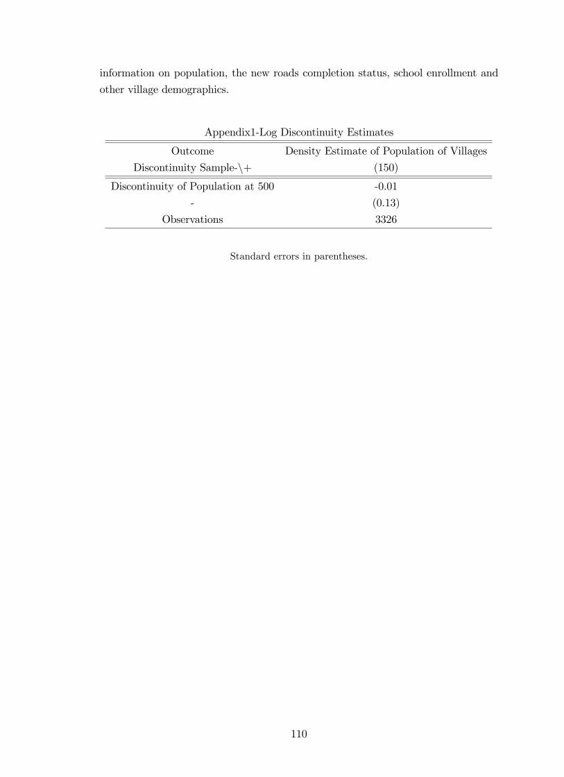
information on population, the new roads completion status, school enrollment and
other village demographics.
Appendix1-Log Discontinuity Estimates
Outcome Density Estimate of Population of Villages
Discontinuity Sample-n+ (150)
Discontinuity of Population at 500 -0.01
- (0.13)
Observations 3326
Standard errors in parentheses.
110

Appendix2-Mid-DayMealSchemeAcrossYears.
111

Appendix3-Comparison of Child Labour for Sample States with National Average
Child Workforce Participation Rates
States (5-9) (10-14) (5-14)
Andhra Pradesh 0.56 12.38 6.61
Kerala 0.00 0.39 0.20
Madhya Pradesh 0.14 5.74 2.82
Rajasthan 0.41 9.42 4.86
India 0.26 6.38 3.33
Source:Derived from Unit Level Records of NSS, 2004-05.
5.2 Appendix to Section 3
5.2.1 Calculating the E¤ective Fringe Bene�t Tax-Rate of Firms
This appendix describes the procedure for calculation of the e¤ective tax rate a
�rm faces in each industry. The e¤ective tax rate FBik on each expenditure head is
computed by using the following formula for the �rm:
FBik = [TBk � TRi] ; i = firm; k = exp enditure head:
where TBk is the FBT base rate for a particular expenditure i.e. percentage of
the total expenditure head considered for tax calculation. TRi represents the tax rate
for a particular �rm respectively
112

A1-E¤ectiveRatesofFringeBene�tTaxforDi¤erentF�rmsandDi¤erentExpenditureHeads@
Sector
FBTBaseRate(%ofexpenseincurred)
TaxRate
Hospitality
Travel
Hotel
RepairESOP
Others
Domestic
Non-Domestic
Cooptv.
Airline,Air-cargo
520
50
100
2033.99
31.67
30.9
Construction
205
2020
100
2033.99
31.67
30.9
ComputerSoftware
205
520
100
2033.99
31.67
30.9
Hotel
520
2020
100
2033.99
31.67
30.9
Pharmaceuticals
205
520
100
2033.99
31.67
30.9
Shipping
520
520
100
2033.99
31.67
30.9
MotorVehicles
2020
205
100
2033.99
31.67
30.9
Others
2020
2020
100
2033.99
31.67
30.9
Source-Compiledfrom
Kishore(2008)andSections115W
B,115WCofIncomeTaxActandAssortedBudgetIssues.
@Thee¤ectiverateistheproductoftheValuationBaseRateandtheFirm�sTaxRate.The�rm�sTaxrateisthetaxrateitfacesaccordingto
incometaxstatus.Foreignownership�rmsareassumedtohaveNon-domesticStatusforsimpli�cationbutinrealitysomeofthem
mayenjoythe
domesticstatus.ESOPandtheSuperannuationFund(Ins)areclubbedtogetherastheyhavethesamee¤ectivetaxrate.Travelandconveyance
areclubbedtogether.
113

5.2.2 Data Appendix
De�nition of Expenditure for consideration of Fringe Bene�ts TaxExpenditure on Lodging: The fringe bene�ts shall be deemed to have been
provided by the employer to his employees, if the employer has, in the course of his
business or profession (including any activity whether or not such activity is carried
on with the object of deriving income, pro�ts or gains) incurred any expense on, or
made any payment foruse of hotel, boarding and lodging facilities.
Expenditure on Travel: The fringe bene�ts shall be deemed to have been
provided by the employer to his employees, if the employer has, in the course of his
business or profession (including any activity whether or not such activity is carried
on with the object of deriving income, pro�ts or gains) incurred any expense on, or
made any payment for conveyance, tour and travel (including foreign travel).
Contribution to Superannuation Fund: Any contribution by the employerto an approved superannuation fund for employees.
Annual Survey of Industries(ASI)Workers are de�ned to include all persons employed directly or through any
agency whether for wages or not and engaged in any manufacturing process or in
cleaning any part of the machinery or premises used for manufacturing process or in
any other kind of work incidental to or connected with the manufacturing process or
the subject of the manufacturing process . Labour engaged in the repair & mainte-
nance, or production of �xed assets for factory�s own use, or employed for generating
electricity, or producing coal, gas etc. are included.
Employees include all workers de�ned above and persons receiving wages andholding clerical or supervisory or managerial positions engaged in administrative of-
�ce, store keeping section and welfare section, sales department as also those engaged
in purchase of raw materials etc. or purchase of �xed assets for the factory as well as
watch and ward sta¤.
Total Persons Engaged include the employees as de�ned above and all workingproprietors and their family members who are actively engaged in the work of the
factory even without any pay, and the unpaid members of the co-operative societies
who worked in or for the factory in any direct and productive capacity. The number
of workers or employees is an average number obtained by dividing mandays worked
by the number of days the factory had worked during the reference year.
Wages and Salaries are de�ned to include all remuneration in monetary termsand also payable more or less regularly in each pay period to workers as compensation
for work done during the accounting year. It includes (a) direct wages and salary (i.e.,
basic wages/salaries, payment of overtime, dearness, compensatory allowance, house
rent and other allowances), (b) remuneration for the period not worked (i.e., basic
114

wages, salaries and allowances payable for leave period, paid holiday, lay-o¤payments
and compensation for unemployment, if not paid from sources other than employers),
(c) bonuses and ex-gratia payment paid both at regular and less frequent intervals
(i.e., incentive bonuses, good attendance bonuses, productive bonuses, pro�t sharing
bonuses, festival or year-end bonuses, etc.). It excludes lay o¤ payments which are
made from trust or other special funds set up exclusively for this purpose i.e., pay-
ments not made by the employer. It also excludes imputed value of bene�ts in kind,
employer�s contribution to old age bene�ts and other social security charges, direct
expenditure on maternity bene�ts and crèches and other group bene�ts. Travelling
and other expenditure incurred for business purposes and reimbursed by the employer
are excluded. The wages are expressed in terms of gross value i.e., before deduction
for �nes, damages, taxes, provident fund, employee�s state insurance contribution,
etc.
Contribution To Provident Fund And Other Funds includes old age bene�tslike provident fund, pension, gratuity, etc. and employers contribution towards other
social security charges such as employees state insurance, compensation for work
injuries and occupational diseases, provident fund-linked insurance, retrenchment and
lay- o¤ bene�ts.
Workmen and Sta¤Welfare Expenses include group bene�ts like direct ex-penditure on maternity, crèches, canteen facilities, educational, cultural and recre-
ational facilities; and grants to trade unions, co-operative stores, etc. meant for
employees.
Total Emoluments is de�ned as the sum of wages and salaries, employers�con-
tribution as provident fund and other funds and workmen and sta¤ welfare expenses
as de�ned above.
Center for Monitoring Indian Economy (CMIE)Sales refer to the sum of industrial sales and income from non-�nancial services.
This �eld re�ects what most non-�nance companies would report as Sales or Income
from its main activities. It includes the income the company earned through the sale
of industrial goods and its various associated incomes such as sale of scrap or raw
material or through providing job-work, utitility services, trading or other services.
It includes all kinds of incomes that the company may earn through the providing of
all kinds of non-�nancial services.
Salaries and wages refer to the periodic payments made to the employees forthe services rendered by them.
Superannuation Fund: Contribution to the provident fund has been considerdsimilar as superannuation fund. The "Employees Provident Fund Act" mandates
that employers are required to make a contribution, in favour of the employees, to
the Provident Fund Account an amount equal to 12 per cent (earlier 10 per cent) of
115

the basic pay and dearness allowance. This is a statutory requirement essentially to
save for the post-retirement life of employees. Any amount that is contributed by the
employer during the year to this account is reported by the companies as contribution
to Provident fund.
Director�s Remmuneration:The remuneration paid to directors which is re-ported under this data�eld includes the amount of salary paid, contribution to prov-
ident fund, value of perquisites, performance linked incentive to whole time directors
and also the commission paid to them.
5.3 Appendix to Section 4
5.3.1 Data Appendix
Glossary of Pradhan Mantri Grammen Sadak Yojna (PMGSY)All-weather road: A road which is negotiable during all weathers, except at ma-
jor river crossings. This implies that the road-bed is drained e¤ectively by adequate
cross-drainage structures such as culverts, minor bridges and causeways. Interrup-
tions to tra¢ c as per permitted frequency and duration are, however, allowed. The
pavement should be negotiable during all-weather, but this does not necessarily imply
that it should be paved or surfaced or black-topped.
Black-Topped Road (BTR): A road provided with bituminous surfacing.Core Network: Network that is essential to provide basic access to each habita-
tion. It can also be de�ned as the network of all the Rural Roads that provide Basic
access to all the Habitations. Basic access is de�ned as the single all-weather road
connectivity to each Habitation. As already indicated, the e¤ort under the PMGSY
is to provide single all-weather road connectivity to each Habitation by way of con-
necting it to another Habitation having all-weather connectivity or to an all-weather
road, in such a way that there is access to, inter alia, Market Centers.
Gravel Road (GR): A road constructed using well compacted crushed rock orgravel material, which is fairly resilient and does not become slippery when wet.
Habitation: A cluster of population, living in an area, the location of which doesnot change over time. Desam, Dhanis, Tolas, Majras, hamlets etc. are commonly
used terminology to describe the Habitations. A Revenue village/ Gram Panchayat
may comprise of several Habitations.
New Connectivity: The construction of roads on the existing alignments fromearth-work stage.
Paved Road (PR): A road provided with a hard pavement course, which
should be at least a water-bound-macadam layer. A paved road need not necessarily
be surfaced or black-topped.
Unconnected Habitation: A habitation with a population of more than 500
116

persons and located at a distance of at least 500 meters (0.5 km) ( from an all-weather
road or a connected village/habitation).
Unpaved Road (UPR):A road not having a hard pavement course (which
should be at least a water-bound-macadam layer). Thus, earthen road and gravel
road will be unpaved roads.
Village Roads (VR): These are roads connecting villages/Habitation or groupsof Habitation with each other and to the nearest road of a higher category.
Water Bound Macadam (WBM): This is the road layer made of crushedor broken aggregate mechanically interlocked by rolling and the voids �lled with
screening and binding material with the assistance of water.
Primary Data Construction Process from PMGSY, Concording to Cen-sus 2001 Village Directory and Statistical Report on General Elections,1999.Step1: The Core Network (CN) provides information on all eligible habitations
with a population over 100 which satisfy the distance criteria. Each habitation in
CN has been assigned a unique 10 digit code with �rst two -state, next two-district,
next two-block and last four habitations by PMGSY. This provides the population
information (according to 2001 Census) ,connectivity status (unconnected for new
connectivity ) of these habitations and 2001 Census villages from which they were
drawn.
Step 2: The Completed Road and Proposed Roads status is provided in the Dis-
trict Pro�le, which has a unique project or road code. The Completed Road informa-
tion does not provide any habitation information but the proposed road information
does. So merging the Completed Roads with Proposed roads would provide the dis-
tricts, blocks and habitations name where the roads have been completed.
Step 3: The PMGSY Block and District code has to be concord with that from
the census �le to obtain their respective 2001 Census codes and names.
Step 4: The proposed road whose subset has been completed should be merged
with the CN for a 1:1 mapping of the habitations and their completed roads status
(or new roads status). Further, this allows forming the unique 16 digit village 2001
Census codes to which this habitation belongs. This allows the use of information
from the census village directory.
Step 5: The new roads dummy variable has been constructed which assigns 1 if the
road construction of a habitation is completed and zero if either under construction
or not proposed.
Step 6: To rectify for manipulation of the habitation population information the
respective census 2001 village total population is used as upper bound.
Step 7: The crude manipulation index is constructed by considering the percentage
of hamlets in the districts as reported in the PMGSY with population at least 500
117

out of total hamlets in the sample.
Step 8: The election constituencies are concorded with 4digit 2001 Census districts
with the help of Delimitation Act.
Step 9: The political alignment dummy variable has been constructed which as-
signs 1 if the incumbent�s political alignment is same as that of the ruling party of
the state considered and 0 otherwise. For assigning the ruling party a rule of thumb
used is that the party has to win at least �fty percentage of the total constituencies
in the state. If none of the parties won by the rule of the thumb then it is assumed
that the majority parties formed a coalition.
Step 10: Finally, the two data sets have to be merged on the basis of 4 digit
2001 Census code to get a master data whose unit of observation is the district with
information on crude manipulation for road policy, the average incumbents�political
alignment and the voting margin by which the candidates�won and other district
demographics.
Appendix-McCrary test for various States
States McCrary t Statistic
Cuto¤ 250 Cuto¤ 500
Andhra Pradesh -1.01 -0.39
Rajasthan -3.37 -1.18
Kerala -1.12
Madhya Pradesh 1.87 0.20
Tamil Nadu 0.79 4.65��
Maharashtra 12.49��
4.77��
Chhattisgarh 4.82��
6.60��
Gujarat 6.95��
8.52��
West Bengal -0.73 11.82��
**(5% signi�cance level)
118

Distribution of Habitations for at (250,500)
Thresholds for Maharashtra
119

6 References
1. Angrist, Joshua, Lavy, Victor, 1999. Using Maimonides�Rule To Estimate The
E¤ect of Class Size on Scholastic Achievement. Quarterly Journal of Economics,
114 (2) , 533-575..
2. Assorted Issues of Annual Survey of Industries, India
3. Assorted Issues of Union Budgets, India.
4. Assorted Reports of Pradhan Mantri Gram Sadak Yojana, India
5. Assorted Reports of Statistical Report on General Elections, 1999, India.
6. Alesina, A, Baqir, R., Easterly, W, 1999. Public Goods and Ethnic Divisions.
The Quarterly Journal of Economics, Vol. 114.(4), 1243-1284.
7. Banerjee, Abhijit, 2004. Who is Getting the Public Goods in India: Some Evi-
dence and Some Speculation. in Kaushik Basu (ed), India�s Emerging Economy
: Performance and Prospects in 1990s and Beyond , MIT Press.
8. Banerjee, Abhijit, Somanathan, Rohini, 2007. The Political Economy of Public
Goods : Some Evidence from India. Journal of Development Economics, Vol.
82 (2), 287-314.
9. Banerjee, Abhijit, Iyer, Lakshmi, Somanathan, Rohini, 2008. Public Action
for Public Goods. Handbook of Development Economics, Vol. 4,Chapter 49,
3119-3154.
10. Baltagi, Badi.H., 2009. Econometric Analysis of Panel Data, John Wiley and
Sons Ltd.
120

11. Basu, Kaushik, 1999. Child Labour: Cause, Consequence, and Cure, with
Remarks on International Labor Standards. Journal of Economic Literature,
Vol. 37, 1083-1119.
12. Basu, Kaushik, 2004. The Indian Economy: Up to 1991 and Since. in Kaushik
Basu (ed), India�s Emerging Economy : Performance and Prospects in 1990s
and Beyond , MIT Press.
13. Baum, Christopher F., Scha¤er, Mark E., Stillman, Steven, 2007. Enhanced
Routines for Instrumental VariablesnGeneralized Method of Moments Estima-
tion and Testing. The Stata Journal , Vol. 7 (4), 465-506.
14. Bramati, Maria Caterina., Croux,Christophe., 2007. Robust Estimators for the
Fixed e¤ects Panel Data. Forthcoming in The Econometrics Journal.
15. Bell, Clive, 2010. Goods, Education and Health: A Combined Model for Eval-
uating PMGSY. University of Heidelberg, Germany.
16. Card, David, Chetty, Raj, Weber, Andrea., 2007. Cash-on-Hand and Compet-
ing Models of Intertemporal Behavior: New Evidence from the Labor Market.
The Quarterly Journal of Economics, Vol. 122 (4), 1511-1560.
17. Carrell, Scott E., Hoekstra, Mark, West, James E., 2010. Does Drinking Impair
College Performance? Evidence from a Regression Discontinuity Approach.
NBER Working Paper No. 16330.
18. Census of India Village Directory,2001.
19. Du�o, Esther, 2001. Schooling and Labor Market Consequences of School Con-
struction in Indonesia: Evidence from an Unusual Policy Experiment. The
121

American Economic Review, Vol 91 (4), 795-813.
20. Dre�ze, Jean, Kingdon, Geeta Gandhi, 1998. Biases in education statistics. The
Hindu, March 6.
21. Epstein, J, Kavweit, N., 1983. Friends in School: Patterns of Selection and
In�uence in Secondary Schools. Academic Press, New York.
22. Filmer, Deon, 2007. If you build it , will they come ? School availability and
school enrollment in 21 poor countries. Journal of Development Studies,Vol. 43
(5),.901-928.
23. Foster, A.D., Rosenzweig, M. R., 1996. Technical Change and Human Capital
Returns and Investments: Evidence from the Green Revolution. American
Economic Review, Vol. 86 (4), 931-953.
24. Foster, A.D., Rosenzweig, M. R., 2000. Technical Change and Distribution of
Schooling: Evidence from the Green Revolution. Working Paper.
25. Freeman, Richard B., 1978. The E¤ect of Trade Unionism on Fringe Bene�ts.
NBER working paper 272.
26. Grossman, S J., Hart,O.D., 1980. Takeover bids, the free-rider problem, and
the theory of the corporation The Bell Journal of Economics , Vol 11, 42�64.
27. Gruber, J., Poterba,J., 1994. Tax Incentives and the Decision to Purchase
Health Insurance:Evidence from the Self-Employed. The Quaterly Journal of
Economics, Vol 109 (3), 701-733.
28. Handa, S., 2002. Raising Primary School Enrollment in Developing Countries:
122

The Relative Importance of Supply and Demand. Journal of Development Eco-
nomics, Vol. 69 (1), 103�128.
29. Holmes,J., 2003. Measuring the determinants of school competition in Pakistan:
Analysis of censoring and selection bias. Economics of Education Review, 22,
249-264.
30. Imbens, Guido, Lemieux, Thomas, 2008. Regression Discontinuity Designs: A
Guide to Practice. Journal of Econometrics, Vol. 142 (2), 615-635
31. Income Tax on Fringe Bene�ts, Chapter XIIH, Section 115W, 115WA, 115WB
and 115WC.
32. Jalan, J., Glinskaya, E., 2003. Improving Primary School Education in In-
dia: An Impact Assessment of DPEP-Phase I. Unpublished Document, Indian
Statistical Institute (New Delhi) and The World Bank.
33. Jacoby, H. G., 2000. Access to Markets and the Bene�ts of Rural Roads. Eco-
nomic Journal, 110 (465), 713�737.
34. Jacoby, H. G., Minten, Bart, 2008. On Measuring the Bene�ts of Lower Trans-
port Costs. World Bank Working Paper, 4484.
35. Jensen, M.C., 1986. Agency Costs of Free Cash Flow, Corporate Finance and
Takeovers. American Economic Review, 76, 323�329.
36. Jhanwar, C.L, 2005. The Finance Bill 2005 �Two New Taxes �Fringe Bene�t
Tax and Banking Cash Transaction Tax. Chartered Accountant, Vol 53, No 9,
1152-55.
123

37. Kishore, Praveen., 2009. Analysis of Fringe Bene�ts Tax and its Collection
Pattern. Economic and Political Weekly, Vol 43, No 33, Issue 16-22, 41-51.
38. Kishore, Praveen., 2009. Collection Trends, Classi�cation of Expense Heads
and Avoidance of Fringe Bene�ts Tax. Economic Political Weekly, Vol 44 (1),
Issue 03-09, 59-67.
39. Lee, David S., Lemieux, Thomas, 2009. Regression Discontinuity Designs in
Economics. Journal of Economic Literature, American Economic Association,
Vol. 48 (2), 281-355.
40. Long, James E., Scott, Frank A., 1982. The Income Tax and Nonwage Com-
pensation. Review of Economic Statistics, Vol 64, 211-219.
41. Marby, Bevars., 1973. The Economics of Fringe Bene�ts. Industrial Relations,
Vol 12, 95-106.
42. Marquis, M.Susan., Phelps,Charles E., 1987. Price Elasticity and Adverse Selec-
tion in the demand for Supplementary Health Insurance. Economic Enquiry,Vol
25, 299-313.
43. McCrary, Justin, 2008. Manipulation of the Running Variable in the Regression
Discontinuity Design: A Density Test. Journal of Econometrics. Vol. 142 (2),
698-714.
44. Mukul, Akshaya, 2009. Dalit kids cannot use school loo but have to clean them.
The Times of India, June 25
45. Oi, Walter Y.,.Iddson,Todd L., 1999. Firm Size and Wages. Hanbook of Labour
Economics,Vol 3, Chapter 33.
124

46. http://pmgsy.nic.in/
47. http://pmgsy.nic.in/downloads/esmf.pdf
48. Royalty, Anne Besson , 2000. Tax preferences for fringe bene�ts and workers
eligibility for employer health insurance. Journal of Public economics, Vol 75,
209-227.
49. Rajan, Raghuram G., Wulf,Julie ,2006. Are Perks Purely Managerial Excess?.
Journal of Financial Economics, Vol 79 (1), 1-33.
50. Sloan, Frank., Adamache,Killard., 1986. Taxation and the Growth of Nonwage
Bene�ts. Public Finance Quaterly, Vol 14, 115-139.
51. Taylor, Amy., Wilensky,Gail., 1983. The E¤ect of Tax Policies on Expenditures
for Private Health Insuranc in Jack Meyer,ed., Market Reforms in Health Care:
Current Issues and New Directions,Strategic Decisions.
52. Turner, R.W., 1987. Are Taxes Responsible for the Growth in Fringe Bene�ts?.
National Tax Journal XL2, 205-220.
53. UNICEF 2006. Social exclusion of Scheduled Caste Children from Primary
Education in India, UNICEF, India.
54. Ward, Michael (2007). Rural Education. India Infrastructure Report.
55. Wills, Robert J, 1986. Wage Determinants: A Survey and Reintterpretation of
Human Capital Earnings Functions. Handbook of Labor Economics, Vol. 1,
Chapter 10, 525-602.
125

56. Woodbury, Stephen A., 1983. Substitution Between Wage and Non-Wage Ben-
e�ts. American Economic Review, Vol 73 (1), 166-82.
126
7 Vitae
MUKTA MUKHERJEE
EDUCATION
Ph.D, Economics, Syracuse University, 2008, Spring -2012
M.A., Economics (CGPA 3.5/4), State University of New York, Albany, 2005-2007
M.Phil, Economics, First class, Delhi School of Economics, India, 2002-2005
M.Sc, Economics, First class (8th Rank), Calcutta University, India, 1999-2001
B.Sc, Economics, Lady Brabourne College, India, 1996-1999
FIELDS OF INTEREST
Labor Economics, Public Economics, Development Economics
PUBLICATIONS
Alam, Moneer and Mukherjee, Mukta (2008), �Ageing, Activities of Daily Living
Disabilities and the Need for Public Health Initiatives: Some Evidence from a House-
hold Survey in Delhi�; in Chopra, Kanchan and C.H. Hanumantha Rao (eds), Growth,
Equity, Environment and Population: Economic and Sociological Perspectives, pp.
369-91, New Delhi:Sage Publications.
Rajaraman, Indira and Mukherjee, Mukta (2006), �Predicting the Probability
of Default on Bank Loans & NPAs� ; The Empirical Economics Letters 5:3(May);
171-180.
Alam, Moneer and Mukherjee, Mukta (2005), �Ageing, Activities of Daily Liv-
ing Disabilities and the Need for Public Health Initiatives: Some Evidence from a
Household Survey in Delhi�; Asia-Paci�c Population Journal. 20 (2), pp.47-76.
PAPER PRESENTATION
Delhi School of Economics, Delhi, India, January 2011
127

7th Annual Conference on Growth and Development, Indian Statistical Institute,
Delhi
TEACHING EXPERIENCE
Department of Economics, Syracuse-University, 2008-2011
Instructor-Economic Ideas and Issues-Summer 2010, 2011
Teaching Assistant-Mathematics for Economists (Ph.D. level), Game Theory (Mas-
ters level)
Economics Ideas and Issues (Under-graduate level)
Department of Economics, SUNY Albany, 2005-2007
Teaching Assistant- Econometrics (Ph.D. level), Microeconomics (Under-graduate
level)
WORK EXPERIENCE
Internship in Econometric Research Institute, SUNY Albany, Summer 2006
Research Analyst and Research O¢ cer, Institute of Economic Growth, Delhi,
India, 2002-2005.
HONORS AND AWARDS
Future Professoriate Program, 2010
Maxwell Summer Research Fellowship, 2010
Roscoe Martin Research Grant for Doctoral Dissertation, 2010
Graduate Assistantship at Syracuse University, 2008- 2012
Teaching Assistantship at SUNY, Albany, 2005-2007
Ranked First in the All India Entrance Test for M.Phil, 2002
Amita Memorial Scholarship in M.Sc, 2001
128