The Effects of EU’s Subsidised Export on Developing Countries

The Case of Dairy Products

Bachelor’s Thesis within Economics

Author: Tina Alpfält

Cathrine Roos

Tutor: Johan Klaesson, Associate Professor

Hanna Larsson, Ph. D. Candidate

Jönköping January 2010

Bachelor’s Thesis in Economics

Title: The Effects of EU’s Subsidised Exports on Developing Countries

The Case of Dairy Products

Author: Tina Alpfält, Cathrine Roos

Tutor: Johan Klaesson, Hanna Larsson

Date: 2010-01-18

Subject terms: CAP, EU, subsidies, developing countries, agriculture, dairy

Abstract

The purpose of the thesis is to examine the effect EU’s subsidised dairy export has

on developing countries’ dairy production. This is done by constructing a model

containing various factors that are assumed to affect production. Data was

collected for 23 countries in Africa, Central- and South America and was pooled

together using a least squared dummy variable model (LSDV). The variable of

interest for this study is the imports from EU to the selected countries. The

regression result showed that this variable was negatively correlated with the

countries’ domestic dairy production and was significant on the 1% level

confirming the hypothesis of the variable. Due to the negative correlation, a

reduction of the EU exports is thus assumed to increase these countries’ own

production within this agricultural sector. As shown in the thesis, agriculture is

important for a country’s development and hence, by exporting subsidised goods,

EU might hinder development in the countries studied. However, over the years

the EU has received a lot of pressure from the WTO to decrease its domestic- and

export subsidies. Due to this, the EU has promised, based upon certain conditions,

to remove its export subsidies completely by 2013. This is seen as positive for the

developing countries’ future development prospects.

Acknowledgments

We would like to thank our tutors Associate Professor Johan Klaesson and

Ph. D. Candidate Hanna Larsson for all valuable assistance during the work

process. We would also like to thank Fabian Nilsson, Andreas Davelid and

Harald Svensson from the Swedish Board of Agriculture for their time spent

assisting our search for information regarding subsidies.

i

Contents

1. Introduction ............................................................................ 1

1.1. Previous Research ........................................................................ 2 1.2. Problem & Purpose ....................................................................... 3 1.3. Limitations ..................................................................................... 4

1.4. Disposition ..................................................................................... 4

2. Growth and Agriculture ........................................................ 6

3. The Common Agricultural Policy (CAP) ............................. 7

3.1. The History and Development of CAP ........................................... 7 3.2. The Goals of CAP ......................................................................... 8

3.2.1. The Tools of CAP ............................................................... 9

3.2.2. The Winners and Losers ................................................... 10

3.3. The Dairy Sector within the EU ................................................... 11

4. The World Trade ................................................................. 13

4.1. Agreement on Agriculture(AoA)................................................... 13

4.2. Anti-dumping ............................................................................... 15

5. Trade Theory ....................................................................... 16

5.1. Comparative Advantages ............................................................ 16

5.2. Effects on the Market of Domestic Subsidies .............................. 16 5.3. Export Subsidies & Imperfect World Markets .............................. 17 5.4. Supply Shock for the Importing Country ...................................... 19

5.5. Additional Factors Affecting Production ....................................... 20

5.6. Summary ..................................................................................... 21

6. Empirical Section ............................................................... 22

6.1. Presentation of Model and Variables........................................... 22

6.2. Additional Assumptions ............................................................... 23 6.3. Econometric Method ................................................................... 24

6.4. Descriptive Statistics of the Model Variables ............................... 25 6.5. Output of the Regression Model .................................................. 26 6.6. Analysis ....................................................................................... 27

7. Conclusion .......................................................................... 29

List of references ..................................................................... 30

ii

Figures Figure 1.1 Thesis outline ............................................................................. 5 Figure 3.1 EU’s export of dairy products .................................................... 12 Figure 5.1 The effects of a price floor in a market ..................................... 17 Figure 5.2 Welfare effects of an export subsidy. ........................................ 18

Figure 5.3 Effects of a supply shock for the importing country. .................. 19 Figure 5.4 Engel curve for a normal good .................................................. 21

Tables Table 3.1 Yearly costs of CAP and export subsidies ................................. 10 Table 5.1 Distribution of welfare from an export subsidy within EU ........... 18 Table 5.2 Distribution of welfare from an export subsidy for the importing

country ....................................................................................... 20 Table 5.3 Hypotheses ................................................................................ 21 Table 6.1 Descriptive statistics .................................................................. 25 Table 6.2 Regression output ...................................................................... 26

Appendices Appendix 1 ................................................................................................... 33 Appendix 2 ................................................................................................... 34 Appendix 3 ................................................................................................... 35 Appendix 4 ................................................................................................... 36 Appendix 5 ................................................................................................... 37 Appendix 6 ................................................................................................... 38

1

1. Introduction

‖ The absurdity of the situation in the agricultural markets is the following: The rich

countries, that is, the EU and the USA give subsidies to the farmers for the production

and export of their produce last year to the tune of 349 billion dollar/…/ the

consequences of that are dumping, the destruction of agriculture in the southern

hemisphere where there is almost nothing else apart from peasant agriculture/…/. So

the Senegalese peasant/…./ hasn’t got a chance of being able to survive by working his

own land. So what can he do? If he’s still got the energy he risks his life as an illegal

immigrant via the straits of Gibraltar and has to hire himself out somewhere or other in

southern Spain or work as a street sweeper in Paris in inhumane conditions.‖

Jean Ziegler, UN special Rapporteur on the right to food (Grasser, 2005)

The situation outlined above is a description of the world today. The European Union

(EU) has developed a Common Agriculture Policy, known as CAP. This policy gives

the European farmers large amount of subsidies, which during the 21st century has

accounted for 40-50% of the total EU budget (European Commission, 2010). The

subsidies are said to create incentives for overproduction and the EU encourages export

of the excess food, by granting export subsidies. The export subsidies enable European

farmers to sell their products on the world market to prices below their production cost.

This contributes to an unfair world trade where the developing countries’ export cannot

compete with the developed countries’ subsidised export; even though their production

costs in many cases are lower (Oxfam, 2005).

The subject is widely debated in media today and the European Union has received a lot

of criticism for its agricultural policy (Seth, 2004). Due to world trade policies, decided

within the World Trade Organisation (WTO), the EU has discussed a removal of their

export subsidies by 2013 (Agebjörn, 2007) and to make their agriculture more adapted

to the market forces. Consequently, last year the EU farmers were protesting against the

higher production quotas on dairy products in Brussels (SVT, 2009).

Within the EU, the light is shed mostly on the domestic consequences from CAP,

however what about the consequences outside the EU? The thesis will investigate

whether a relationship between the European subsidised exports and the production in

developing countries can be seen. In those countries the main source of income comes

from farming (Oxfam, 2005) and when these local farmers are driven out of business by

cheap imports, they often do not have any other work opportunities. This has not only

devastating effects for the affected farmers but also on the countries’ future

development prospects (Sarris, 2001).

The effects of the European agricultural policy are important to scrutinise due to its high

costs to the European taxpayer, last year it amounted to 53.54 billion Euros (European

Commission, 2009a). Additionally, it is claimed by many to have substantial costs for

the developing countries (Matthews, 2008). As pointed out by Ziegler (Grasser, 2005)

his also results in other problems, such as illegal immigration. Hence CAP is not only

an issue for European politicians and farmers.

2

1.1. Previous Research Several studies and analyses have been carried out on the subject of domestic- and

export subsidies within the agricultural sector. Most of the studies regarding liberalising

agricultural world trade have been in the context of measuring the effects of the Doha

Round, the ongoing world trade negotiations within the WTO. Diao, Roe and Somwaru

(2002) found that eliminating domestic support, export subsidies and agricultural tariffs

worldwide, would cause agricultural prices to rise by an average of 12%. About half of

that increase would be due to liberalising agricultural trade in EU and the EFTA1,

whereas Japan, Korea, Canada and the United States would account for approximately

the remaining half of this expected price increase. Diao et al. (2002) attributes this

finding to three major reasons: those countries are all major players on the world

agricultural market, they impose high tariffs on a few agricultural products and they use

support policies, such as export subsidies in the case of the EU. As many developing

countries’ export markets are located in a few countries in ―the north‖, they found that

the majority of developing countries would benefit from a more open EU agricultural

market. Diao et al. (2002) came to the conclusion that in the short-run, the welfare

effects will be rather low for developing countries but recognised that agricultural trade

reforms would increase production in developing countries, which would lead to an

increased trade volume and hence an increased welfare over time. Their results propose

that, following such trade reform, all developing countries would benefit in the long-

run.

Frandsen, Gersfeldt and Jensen (2003) conducted a study where they analysed three

scenarios to show the impacts of decoupling or eliminating the EU agricultural support.

They found that the EU domestic support did affect production decisions and hence

distorted international trade. This in turn showed to have negative effects on the export

potential of developing countries. Hence, their conclusion was very much in line with

that of Diao et al. (2002).

That the EU’s domestic support is stated not to affect production decisions, due to

being decoupled, is found by many to be highly unlikely due to the large amount money

spent by EU on CAP2 (Matthews, 2008; Bureau, Jean and Matthews, 2006). This was

also confirmed by the study conducted by Frandsen et al. (2003). Matthews (2008)

found that reducing export subsidies, ending production subsidies and removing

protection would generally be welcomed by developing countries. For those countries

that have export capacity in products that receive support by the CAP, the EU farm

policy is considered especially harmful as it constitutes unfair competition on the world

market. However, whereas local producers in the importing countries always get

damaged by the policies, countries that are net importers of CAP products benefit from

CAP policies in the way that they contribute to lower world market prices and hence

give those countries terms of trade gains on their imports. Consumers of those products

also gain due to cheaper prices. This conclusion was reached by Diao et al. (2002) as

well and explains why they recognised that not all developing countries were immediate

winners of liberalising agricultural trade. Matthews (2008) presents in his research the

often prevailing assumption that consumers that gain from cheaper supplies often are

better off and live in urban areas, whereas those hurt by the subsidised export are the

1 European Free Trade Agreement

2 See table 3.1

3

poorer, rural producers. Whether this is true or not, however, Matthews (2008) states

can only be determined on a case-by-case basis. Even though Matthews (2008) found

that EU farm policy has varied impacts on developing countries, he reaches the overall

conclusion that the aggregate cost of distortion to developing countries from the CAP

policies are greater than the benefits received in certain countries due to cheaper

supplies. Bouët, Bureau, Decreux and Jean (2005) found, in contrast to Diao et al.

(2002) that the ending of export subsidies would only have a limited effect on overall

world prices; only in the dairy- and sugar sector will the reduction have a substantial

effect. However, even though limited, the increase will contribute to an increase in the

food bill of those developing countries that are net importers of food and do not have

resources enough to sufficiently increase their production. Bouët et al. (2002) thus argue

that the general conclusion that developing countries in general will gain from

liberalising agricultural trade could be very misleading as the effects will be very

uneven. Bureau, Jean and Matthews (2006) also conclude, much by using the Bouët et

al. (2005) study, that even though removing export subsidies are necessary to combat

unfair competition, caused by dumping, the overall positive effects must not be

overestimated for developing countries. In addition the consequences, for net food-

importing countries, are negative in the short-run.

Many non-government organisations have emphasised the side effects of CAP on

developing countries. A report by Oxfam (2005) found that in the Dominican Republic,

around 10 000 farmers were thought to have been driven out of business due to EU’s

subsidised export of milk. Additionally, an article by Fokker and Klukist (2000)

published by Forum Syd shows several examples of how local markets in the southern

hemisphere are negatively affected when their farmers are outcompeted by EU’s

subsidised export. The report highlights the policy incoherence occurring within the EU

by showing how a large share, at the same time, of the EU’s budget is given to those

countries to support their economic development.

In a report by McMillan, Peterson Swane and Ashraf (2007) efforts are being made to

analyse whether one can see a connection between developed countries’ subsidies and

poverty in the developing countries. To measure poverty they used average income. A

clear connection between the variables could not be seen, which they partly attributed to

poor data and partly to a poor choice of variables.

1.2. Problem & Purpose The previous literature within this area found various results for the overall net effects

on developing countries of liberalising agricultural world trade. The purpose of this

study is to see to what extent CAP is market distorting for developing countries by

examining the effects of EU exports on local production. This is an important step

towards being able to measure the overall costs of these subsidies in order to determine

the overall net effects across developing countries.

Most previous research has focused on measuring the effects on prices when liberalising

the world trade rather than how harmful CAP is for other countries’ production. A

study, made by Macmillan et al. (2007), attempting something similar tried to measure

the effects on overall poverty and not on production.

4

The EU was chosen as an exporter in this study due to three reasons. Firstly, the EU is

considered as one of the world’s major economic powers and its world trade is assumed

to have a great impact on billions of people (Agebjörn, 2007). Secondly, the EU has an

explicit policy that says that the policies within all its sectors that affect developing

countries should be coherent with its development promoting objectives as stated by the

articles 177 and 178 in the Treaty of the European Union, found in Appendix 1. Lastly,

the EU has received lots of criticism for its subsidised export (Seth, 2004).

Dairy products were chosen as the commodities of interest for this study due to three

reasons. Firstly, the EU is an important actor on the dairy world market; the last fifteen

years the EU was among the top two exporters in the world of whole milk powder, top

two exporters of butter and the leading exporter of cheese (WTO, 2009). Secondly,

today the EU has reduction commitments on all these commodities implying that these

commodities are exported with subsidies. Lastly, dairy products are considered to be

basic commodities.

Developing countries were chosen as importers of dairy products as they are seen as

more vulnerable to the unfair competition export subsidies are said to cause (Grasser,

2005). The focus is on Africa, Central-and South America since they are the ones most

frequently mentioned in previous studies (Fokker and Klukist, 2000; McMillan et al.,

2007). Following this reasoning the problem will be outlined as follows:

Does EU’s subsidised export of dairy products have a negative impact on the

production of cow milk in developing countries, and to what extent is it market

distorting?

1.3. Limitations In the thesis there will be three limitations when investigating the stated problem.

Firstly, the focus will be on the recipient of the European Union’s export and not on the

effects and consequences within the EU. Secondly, even though there are many suitable

countries to investigate the focus will be on those developing countries, shown in

Appendix 2, due to availability of reported data. Lastly, the data will range from the

years 1975 to 2005, due to data availability.

1.4. Disposition

In Figure 1.1., found below, an outline of the structure of the thesis is presented. The

thesis starts with an introduction of the topic together with the purpose and limitations

of the thesis. It continues with the background section which is split into three parts to

provide a deeper understanding of the topic discussed in the thesis. It is followed by the

theory section which outlines and states the hypotheses to be examined in the empirical

section. The major findings of the thesis can be found in last section together with

suggestions for future research.

5

Figure 1.1. Thesis outline

6

2. Growth and Agriculture Agriculture is an important economic sector in the society since it provides food

supplies for its population. However, it is also considered important for development

and growth, which are central issues for developing countries.

As noted by Andreosso-O’callaghan (2003), there seems to be a relationship between

the importance of agriculture in an economy and the level of development. This

relationship is negative, which implies that in highly developed countries agriculture

does not matter much. In poorly developed countries, Andreosso-O’callaghan (2003)

states, the opposite can be seen; a large part of the labour force works with agriculture,

which also makes up a large part of their GDP.

A way of interpreting this could be that poor developing countries should stop focusing

on agriculture and try to develop manufacturing industries and services instead. Some

researchers claim that is not the case, however. For example Rostow (1960) wrote ―The

stages of economic growth‖ in 1960 where he explains that there are five stages,

altogether, of growth. The first stage comprises the traditional society where many

resources are devoted to agriculture since the output cannot become more efficient due

to lack or non-use of modern technologies. The second stage is called the preconditions

for take-off and this is the stage during which the society is being transformed so that it

can start to use modern technologies and enjoy the benefits they bring. Thirdly there is

the take-off itself. An institutional structure is being developed and a steady growth can

be seen in the economy and industries expand rapidly. The fourth stage is the so called

drive to maturity where old industries are being replaced by new ones and the growth

and progress continue to increase. Lastly there is the stage named the age of high mass-

consumption. Here the most important features are the shift from manufacturing to

services and the emergence of the welfare-state.

A similar theory was developed by Bela Balassa in 1977, which discusses the existence

of different stages when it comes to comparative advantages. The structure of a

country’s export depends on the accumulation of capital which is a process that is

constantly changing. As more capital is accumulated and the country gets a comparative

advantage in a new sector it climbs on step further up on the ladder, replacing other

countries. As explained more in detail by Andreosso-O’callaghan (2003), during the

first stage the agricultural production becomes intensified and becomes the core of the

economy. As the development and growth proceeds, the country switches to

manufacturing which now becomes the good of which the country has a comparative

advantage in. In stage three the structure changes in the economy and the focus moves

to more skill-intensive activities. Finally, in the fourth stage services develop and are

now the product for which the country has a comparative advantage.

Both theories show that agriculture is a natural and necessary part of the development

and not to be regarded as something unnecessary that can be omitted. As pointed out by

Andreosso-O’callaghan (2003); we have all been there. As shown by Andreosso-

O’callaghan (2003), most EU countries relied heavily on agriculture 50 years ago, just

like developing countries do today.

7

3. The Common Agricultural Policy (CAP) The Common Agricultural Policy has been in use for over 50 years and is a complex

policy that uses lots of tools to accomplish goals set up in a variety of areas. Examples

are policies regarding fishing and rural development; however, the focus of the section

will be on the policies that directly concerns agriculture. This creates an understanding

for why the present situation has been able to develop and how the EU operates on the

market.

3.1. The History and Development of CAP In the 1950’s when the Treaty of Rome was negotiated agriculture had an important

role. Not many years had passed since the Second World War and the food-shortages

experienced then were to be avoided in the future by helping the involved countries to

become self-sufficient again (European Commission, 2004). In addition, there was a

risk that the country side would become empty when the industries in the cities required

more workers (Altomonte & Nava, 2005). The urbanisation was dangerous in several

ways; partly by the potential problems that could follow from a fast urbanisation and

partly because the food production could become endangered. Hence, something had to

be done to encourage farmers to stay in the agricultural sector.

According to Altomonte and Nava (2005), about 25% of the population in the six

member countries3 were farmers in the 1950’s. In addition, the countries had individual

agricultural policies that were already developed and they were very reluctant to abolish

them. Hence the common agricultural policy (CAP) became a necessary ingredient in

the Treaty on the European Economic Community (EEC) when it was signed in Rome

in 1957.

As explained by El-Agraa (2004) the intention with an economic community was

economic integration. By starting to integrate the agriculture, politicians hoped that a

successful integration would facilitate for the same integration in other sectors of the

society as well.

Only a few years after the establishment of CAP in 1957, the requests of reforms

started. The first big reform being developed was the Mansholt Plan in 1968. The

features of this reform, which was not implemented until 1972, was to actively try to

reduce the number of people employed in the agricultural sector and to promote more

efficient methods and larger sizes of the farms (Altomonte and Nava, 2005). This

reduction in number of farmers was, according to Cardwell (2004), an attempt to

decrease the overproduction that had become evident.

The next big reform made was the Delors I reform which was agreed upon in 1988. It

had three important affects on the agriculture. Firstly, it tried to restrain the growth of

the CAP expenditures; the expenditures could only increase to 74% of the total GNP

increase. Hence more money would be made available for other policy purposes when

the income increased in the area (Altomonte and Nava, 2005). Secondly, the target

prices, export refunds and import tariffs were to be lowered so that the overproduction

would be discouraged. Thirdly, production quotas were also set in place to discourage

overproduction (Altomonte and Nava, 2005). Lastly, as mentioned by Cardwell (2004),

3 The six members can be found in Appendix 3.

8

a set-aside system was introduced, which implies that a part of the land owned by a

farmer is left unfarmed.

The most famous reform is the MacSharry reform from 1992. The reform built a lot on

the Delors I reform from 1988, although it had to be extended so that the other WTO

members would accept it and be willing to close the Uruguay Round4 (Altomonte and

Nava, 2005). This was done by focusing more on direct support than price support,

which was necessary to try to push the markets back in balance (Cardwell, 2004). The

changes made include for example; various cuts in tariffs and target prices, making the

set-aside scheme available to more farmers, making compensations through direct

payments and introducing an early retirement scheme in order to reallocate labour

(Andreosso-O’callaghan, 2003).

The most recent reform of CAP is the Agenda 2000 reform from 1997. The purpose was

to prepare the EU for the big enlargement in 2004 where ten new members joined. The

changes made in the CAP comprised of; further reduction of target prices, a new rural

development policy, more environmental considerations, improvement of the safety and

quality of food and a simplified legislation where the application process was

decentralised to the member countries. This reform was evaluated in 2002 (Altomonte

& Nava, 2005).

During the evaluation, the mid-term review, it was decided that some additional

changes were to be made along the path of less market distorting subsidies (Altomonte

and Nava 2005). The reform was adopted in 2003 and contained the following changes;

direct aid was to be decoupled (independent of the production) and the aid was only to

be given if the farmers complied with certain standards concerning the environment,

food, animals etc. In addition, more resources were to be used for the rural development

and the payments made to bigger farms were reduced in order to decrease the harm they

caused small farms.

3.2. The Goals of CAP When the CAP was created in year 1957, goals were established that the EU should aim

at fulfilling. The goals are stated in the treaty of the European Union in Article 33.

‖1. The objectives of the common agricultural policy shall be:

(a) to increase agricultural productivity by promoting technical progress and by

ensuring the rational development of agricultural production and the optimum

utilisation of the factors of production, in particular labour;

(b) thus to ensure a fair standard of living for the agricultural community, in particular

by increasing the individual earnings of persons engaged in agriculture;

(c) to stabilise markets;

(d) to assure the availability of supplies;

4 One of the negotiating rounds as implemented by the General Agreement on Tariffs and Trade (GATT)

which started in 1986 and closed in 1995.

9

(e) to ensure that supplies reach consumers at reasonable prices.‖

European union — consolidated versions of the treaty on European Union and of the

treaty establishing the European community (EU, 2006, p.54)

3.2.1. The Tools of CAP

In order to fulfil the goals stated in the previous section the EU uses various tools

whereof the most frequently discussed by El-Agraa (2004) are described here. One

could say that there are two categories of tools, one which regulates the internal market

and one which regulates the external trade.

The first method to be discussed is tariffs, which is a tool to control and to put a

lowering pressure on the imports to the EU. An ordinary tariff is a sum that is put on the

price of a good that is being imported, which makes it more expensive. An ad valorem

tariff has the same effect of making the good in question more expensive, although it is

a percentage that is put on the price of the good. Hence, more expensive products pay

higher duties.

Another tool used to regulate imports is quotas which imply that a certain amount of a

good is allowed to enter the EU at a specified condition. For example a good could be

imported at a cheaper tariff rate or without any tariff. In some cases the quota decides

the quantity of the goods allowed to enter, regardless of the tariff the exporter is willing

to pay.

Preferential treatment is given to some countries or regions, which imply that they are

allowed to export goods to the European Union without paying any tariff or paying a

tariff below the general level.

On the exports from the EU, to the rest of the world, the exporters may receive export

subsidies. This money is supposed to compensate for the loss they make since the world

price is lower than the domestic price. Hence the export subsidies could be said to be

equal to PD-PW, where PD represents the domestic EU price and PW represents the world

price.

The second category is the regulations affecting the domestic EU market. The first tool

discussed is the use of intervention purchases, where various agencies are obliged to

buy the excess products on the market; should the price fall below a certain intervention

price level. This is done in order to make the price increase again, due to the smaller

quantity now available on the market.

In this category quotas can be found as well, although in this setting they are called

production quotas and are put in place to restrict the production of a certain good. This

is also done to decrease the quantity available on the market (El-Agraa, 2004).

Set-aside schemes are another method to decrease the production of goods by

decreasing the amount of available land that farmers can use. The measures discussed

help the politicians to keep the price of agricultural goods close to so called target

prices. These prices are determined by decision makers in order to make sure that

farmers earn enough money to be able to live on farming (Altomonte & Nava, 2005).

10

Direct support payments were introduced by the MacSharry reform and are payments

given to farmers based on their potential income, rather than their actual income, in

order to compensate for lost income due to lower target prices. These are meant to be

less market-distorting than then previous price support (El-Agraa, 2004).

3.2.2. The Winners and Losers

Many actors are involved in the functioning of the CAP and many are those who in one

way or another gain or lose from its existence.

The most obvious winner is the European farmer, the actor the policy was made for (El-

Agraa, 2004). There is also another winner, the non-European consumer who manages

to buy cheaper food due to the subsidies given within the EU (Matthews, 2008).

The most obvious loser is the European consumer who pays an artificially high price for

his/her food. In addition, the European taxpayer is a loser since the CAP is founded by

tax money. Below, in Table 3.1., it can be seen how costly the CAP is for the taxpayers.

However, one has to take into account that more countries have joined the union

throughout this period; hence larger sums of money do not necessarily translate to a

higher cost per taxpayer. Additionally, the non-European farmer that produce the same

goods that the EU exports is also considered to lose from the policy, according to

Andreosso-O’callaghan, (2003). The EU uses export subsidies to sell their goods at

lower prices on the world market, which constitutes unfair competition. The amounts

spent on export subsidies and the share of the total CAP expenditure they constitute is

also shown in Table 3.1. As can be seen, the largest amounts were spent on export

subsidies between 1987 and 1993 and the share of CAP devoted to export subsidies has

declined sharply over the years.

Table 3.1. Yearly costs of CAP and export subsidies

Year Cost of CAP in current billions of

Euros

Whereof spent on export subsidies

Export subsidies as share of CAP

1980 11.32 5.70 0.50

1981 11.87 5.21 0.44

1982 13.06 5.05 0.39

1983 16.73 5.56 0.33

1984 19.01 6.62 0.35

1985 20.63 6.72 0.33

1986 23.09 7.41 0.32

1987 23.89 9.38 0.39

1988 27.58 9.93 0.36

11

1989 25.87 9.71 0.38

1990 27.04 7.72 0.29

1991 33.97 10.08 0.30

1992 34.15 9.47 0.28

1993 37.84 10.16 0.27

1994 36.75 8.16 0.22

1995 38.11 7.80 0.20

1996 43.04 5.70 0.13

1997 44.81 5.88 0.13

1998 43.11 4.82 0.11

1999 45.12 5.60 0.12

2000 41.85 5.65 0.13

2001 45.59 3.41 0.07

2002 46.21 3.45 0.07

2003 47.57 3.73 0.08

2004 47.91 3.39 0.07

2005 52.17 3.05 0.06

Source: European Commission (2009a)

3.3. The Dairy Sector within the EU As stated earlier milk is a basic good. Within the EU, about 14% of the farm output

value consists of dairy products (European Commission, 2004). Regarding EU’s

position on the world market, Piccinini and Loseby (2001) state that the EU’s share of

the world trade of dairy products is about 40%. A picture of the EU exports of dairy

products to the countries in this study is seen in Figure 3.1., which shows how the

export varies from year to year to the countries in this study. In Appendix 4, a case

study of the dairy export to three countries; Chile, Nicaragua and Madagascar can be

found which shows even larger variations.

12

Figure 3.1. EU’s export of dairy products (Authors own construction, based on data from

Comtrade).

The EU became self-sufficient in the dairy sector early and ended up with problems due

to overproduction. Since milk is a perishable it cannot be stored for too long and the

intervention purchases that were made were concentrated to milk powder, butter and

certain types of cheese. The solution was to encourage a decrease in milk production

which was done by introducing production quotas for milk in 1984. At the community

level there is a production quota which is divided into two parts; one for sales to

processing companies and one for direct sales. The member countries each have a

quota, whose quantity is determined by a reference period. The individual farmer in

each member country is then given an individual quota that he or she should not exceed.

If that would happen the farmer has to pay a fine (Piccinini & Loseby, 2001).

The quotas are to be increased by 1% annually from 2009 to 2013 in order to provide a

smooth adjustment for the farmers to actual market demand, for when the quotas are

completely removed in 2015 (European Commission, 2009b). As noted earlier the

farmers have been protesting against this increase of quotas and whether the decision to

remove the quotas will be fulfilled in 2015 is uncertain (SVT, 2009).

050

100150200250300350400450500

19

75

19

77

19

79

19

81

19

83

19

85

19

87

19

89

19

91

19

93

19

95

19

97

19

99

20

01

20

03

20

05

Mill

ion

s o

f kg

s

Quantity of EU exports

13

4. The World Trade Today, global trade is rather complex and subject to many specific rules. The section

introduces the Agreement on Agriculture established by the World Trade Organization,

an organisation EU is a member of and hence need to comply with its trading rules

regarding domestic- and export subsidies.

4.1. Agreement on Agriculture (AoA) Before the founding of the WTO

5 in 1995, no specific agreement regarding trade within

agricultural products did exist. The original trade rules established under GATT did

apply to trade within agricultural products; however, it allowed governments to use

import-quotas and to subsidise its agriculture. Specifically, it allowed countries to use

export subsidies which were not allowed for industrial products. As a result, the trade

within agricultural products became much distorted (WTO, 2008). The WTO followed

the subsequent reasoning that when import barriers and domestic subsidies were used,

crops could become more expensive on a country’s internal market. This in turn

encouraged overproduction, creating a surplus needed to be sold elsewhere. If sold on

the world market, export subsidies are needed to cover for the lower price. Countries

that could afford to subsidise its agricultural sector could hence both produce and export

more than they naturally would. This resulted in export subsidy wars between nations,

whereas countries that could not afford to subsidise their goods suffered from unfair

competition (WTO, 2008). A specific agreement, only concerning agricultural goods

was needed, which was created under the Uruguay Round. The agreement regarding

agriculture was the area the member states had most difficulties agreeing on. The United

States (US) and the European Union, two economic powers which have considerably

high and complex agricultural support systems, did not completely agree until the 7th

of

December 1993, one week before the finishing deadline of the Uruguay Round, (Seth,

2004).

The agreement implied regulations of how much domestic support and export subsidies

each member country was allowed to use. Domestic support got categorised into three

different boxes, with each box getting a specific colour. The amber/yellow-coloured box

includes support that needs to be cut back on since it is considered having direct effects

on production and trade. The reduction required was higher for developed countries

than for developing countries, which also were given a longer time span to meet the

requirements. (WTO, 2008). The base years used for the reduction were 1986-88, a

period when the support levels within both the EU and the US was very high. This

implied that both those economies were left with a high share of support they rightfully

were allowed to use within their agricultural industries (Seth, 2004). No criteria of a

minimum reduction per product existed, which implied that countries could increase

support for one product as long as they compensated the increase by reducing its

support even more for another product (Seth, 2004).

The green box includes support only considered to have a minimal impact on trade and

can therefore be used freely. The box includes the decoupled support which are

payments made directly to farmers that are not considered to encourage production

(Seth, 2004). Examples of such support are direct income support and support to

infrastructure, research, disease control and food security (WTO, 2008). The EU, USA

5 WTO was created on the 1

st of January 1995 out of the Uruguay Round, implemented by the GATT.

14

and Japan are considered giving most support of the green kind (Seth, 2004). The last

box has a blue colour and includes support that initially belonged to the amber/yellow

box. This support is allowed without any reductions for now; as long as requirements

exist to limit production and the support level does not exceed the one of the year 1992

(Seth, 2004). The box is said to be specifically designed to suit the EU’s internal

support system and many other members want it abolished (Seth, 2004).

The AoA does not allow export subsidies, however, there are exceptions. Members are

allowed to use them as long as they are listed on a country’s list of commitments (WTO,

2008). Those members are required to cut these subsidies by both a money value and a

quantity value, using 1986-90 as the base level. The quantity reductions were higher for

developed countries than for developing countries (WTO, 2008), like in the previous

case of domestic subsidies in the yellow box. Members that did not use export subsidies

when the AoA took effect are not allowed to start using them. However, the base years

of which the allowed amounts are based on, were years when the EU’s export subsidies

reached a very high level6. This entails that the reduction the EU has to make is not very

large leaving them with a high use of export subsidies they rightfully were allowed to

use. The reduction the developing countries have to make is not expected to make any

difference, as in many cases developing countries have seldom afforded to give

subsidies in the first place (Seth, 2004). EU has not exceeded the allowed amount of

export subsidies, within the dairy sector, they were allowed to use by the WTO from the

1995 AoA agreement. This can be seen in Appendix 5.

The agricultural agreement from the Uruguay Round did not bring about any immediate

consequences. Reasons for that was due to that base years picked allowed for

continuing high domestic support and that important areas such as USA’s export

credits and the EU’s acre- and animal support were not affected by any reduction

requirements (Seth, 2004). Important, however, was that an agreement regarding

agricultural products was created which made further negotiations possible. In 2000, the

negotiations did start again under the Doha Round. A new agreement is not yet reached

but the negotiations are aimed at continuing to reduce and eventually phase out export

subsidies and reducing domestic support that distort trade (WTO, 2008). An agreement

has been difficult to reach as each country’s negotiating proposals mainly includes

abolishing support they do not give themselves and allowing support they do give. EU’s

proposal contains lowering tariffs whilst keeping acre- and animal support. Instead,

USA’s proposal contained abolishing export subsidies but keeping export credits (Seth,

2004). Another reason why problems have arisen is due to the developing countries

demand on the EU and USA to deliver plans of how they will decrease and eventually

remove their trade distorting support within agriculture (Agebjörn, 2007). In the mean

time, the EU and USA have had their main focus on other issues, which led to the

collapse of the meeting in Cancun in 2003. The negotiations started again in 2004 and

under the Hong Kong meeting in December 2005, the EU promised to remove its export

subsidies gradually until 2013, given that particular agreements were reached on a

handful of other issues. Amongst others were rules and clarifications concerning USA’s

export credits.

6 See Table 3.1

15

4.2. Anti-dumping By using export subsidies a company can charge a price lower than it normally charges

on its own market, or sell to a price that does not cover its production costs. In both

cases the company is said to be ―dumping‖ the product (Seth, 2004). Article VI of the

GATT, called The Anti-dumping Agreement, gives a country the right to protect itself

from this behaviour by applying anti-dumping measures. This is done by charging an

extra import duty to bring the price closer to the ―normal value‖ (WTO, 2008).

However, in order to rightfully use this extra import duty, which normally would break

against the WTO principles, the government importing the dumped product has to show

that dumping is taking place and to which extent. This is done by showing how much

lower the exporting price is in comparison to that country’s home market price (WTO,

2008). In addition, the government must also show that dumping is causing injury to the

domestic production. If the margin of the dumping is insignificant, determined as being

less than 2% of the export price, or if the volume of the dumped imports of one country

is less than 3% of total imports of that product, dumping investigations must end

immediately which leaves the country with no right to implement anti-dumping

measures (WTO, 2008).

Even though an anti-dumping law exists, most developing countries do not fully use the

amount of tariffs they rightfully could apply according to the WTO anti-dumping rule.

Matthews (2008) suggests that this could be due to the benefits the dumped products

bring to the food consumers in the country.

16

5. Trade Theory The section provides the theoretical framework needed in order to analyse the predicted

effects policies outlined in section three and four are said to have on dairy production

in developing countries. The theories give suggestions to model variables and their

hypothesised effects.

5.1. Comparative Advantages According to Krugman and Obstfeld (2006) there are two basic reasons for countries to

trade with each other. The first is due to the differences between countries and the

second to economies of scale.

In the early 19th

century, David Ricardo developed the theory of comparative

advantages (McCulloch, 1888). The theory explains how countries can benefit from

their differences by focusing their production on areas where they perform relatively

well. By doing so the surplus can be traded for goods they produce relatively bad.

Focusing their production on fewer goods will enable them to produce more efficiently

at a larger scale, taking advantage of the economies of scale (McDowell, Thom, Frank

and Bernanke, 2006).

According to Bouët et al. (2005), most developing countries have their comparative

advantages within agricultural production. This is consistent with the theory developed

by Balassa (1977), where comparative advantage within agriculture is said to be the first

stage of the development process. The developed countries, such as the US and

countries within the EU have passed this stage and have moved towards development of

services. Despite this the developed countries are the largest exporters of agricultural

products (Diao et al. 2002; WTO, 2009). This is said to be attributed to their use of

domestic- and export subsidies (Oxfam, 2005).

5.2. Effects on the Market of Domestic Subsidies The graph below, Figure 5.1., shows how the tools of the CAP give incentives to

European farmers to overproduce. As previously explained in section 3.2.1.; the

artificially high prices on agricultural products within the EU serves as a price floor.

They have the opposite effect of price ceilings, which promote excess demand, as

explained by McDowell et al. (2006). The graph represents a basic supply and demand

graph, where the quantity demanded and supplied on the market is a function of the

price.

P* and Q* represents the price and quantity produced that would prevail in an

equilibrium situation if the market was free from intervention. When a price floor is

introduced, which is the lowest guaranteed price a producer can receive for its products,

it is set above the equilibrium price (P*). This is shown in the graph by PEU. At this

artificially high price producers will increase their production from Q* to QS to

maximise their profit. The consumers on the other hand, facing higher prices, will

demand less; a move from Q* to QD.

17

Figure 5.1. The effects of a price floor in a market. (Authors own construction, based on Krugman et al, 2006)

This results in an excess supply of agricultural goods on the European market. In order

for this excess supply not to depress the intra-EU prices it must be removed from the

market and this can be done in several ways. The government can purchase and store

the excess goods for a future shortage, or the goods could be exported to the world

market (Altomonte & Nava, 2005). The last option is to destroy the surplus, which is

demonstrated in the movie by Grasser (2005).

5.3. Export Subsidies & Imperfect World Markets This section examines the effects of the second alternative, export of excess supply, as

suggested in section 5.2 but in a setting with export subsidies. An export subsidy is an

amount of money paid to the producer that constitutes the difference between the

domestic and foreign price levels (Krugman & Obstfeld 2006).

As mentioned earlier, in section 3.2.1., the prices within EU are artificially high; hence

a producer cannot expect the same prices when selling its products outside EU. The

export subsidy is then given as compensation to the farmers from the government (El-

Agraa, 2004).

The price and welfare effects from this policy can be seen below in Figure 5.2. In a

setting without any interventions, the price in both the exporting and importing country

would be at PW.

18

Figure 5.2. Welfare effects of an export subsidy (Authors own construction based on Krugman & Obstfeld, 2006).

With the export subsidy in place, the domestic price increases from PW to PEXP and in

the foreign, importing country the reverse can be seen; the price will fall from PW to P

IMP. The resulting welfare effects within the EU are seen below in Table 5.1.

Table 5.1. Distribution of welfare from an export subsidy within EU.

Group affected Area of gain or loss

Producer gain +(a+b+c)

Consumer gain - (a+b)

Government gain -(b+c+d+e+f+g)

Net welfare result -(b+d+e+f+g)

Source: Authors own construction (based on Krugman & Obstfeld, 2006)

As can be seen from Table 5.1., producers gain from this policy, whereas both

consumers and the government have net losses. The producer gain comes from higher

prices received for their products, which in turn is paid by the consumer which hence

experiences a net loss. The government pays out the subsidy but does not receive

anything back in return. The net welfare outcome from the policy is thus negative for

the society as a whole by the amount of the boxes b+d+e+f+g.

The previous discussion of export subsidies had several assumptions built in. The world

market price does not change, only the prices of the exporting- and importing countries

individually. This scenario assumes a world market of perfect competition, implying

that no single country’s export can affect the world price; everyone is a price taker.

However, the world is more complex than that. In order to affect the price in any

market, the actor needs to have a large share of the total trade of the market in question.

Krugman and Obstfeld (2006), WTO (2009) and Piccinini and Loseby (2001) all

conclude that the EU is one of the main exporters when it comes to agricultural

products. As noted in earlier sections, the EU has as much as 40% of the market shares

on the world market of dairy products. From this one can draw the conclusion that the

19

EU is a big actor on the agricultural world market and has price setting power. Hence

these global markets can be said to be imperfectly competitive (McDowell et al, 2006).

The effects seen in this section has been analysed from an EU perspective only. Section

5.4 will show how this policy affects the importing country.

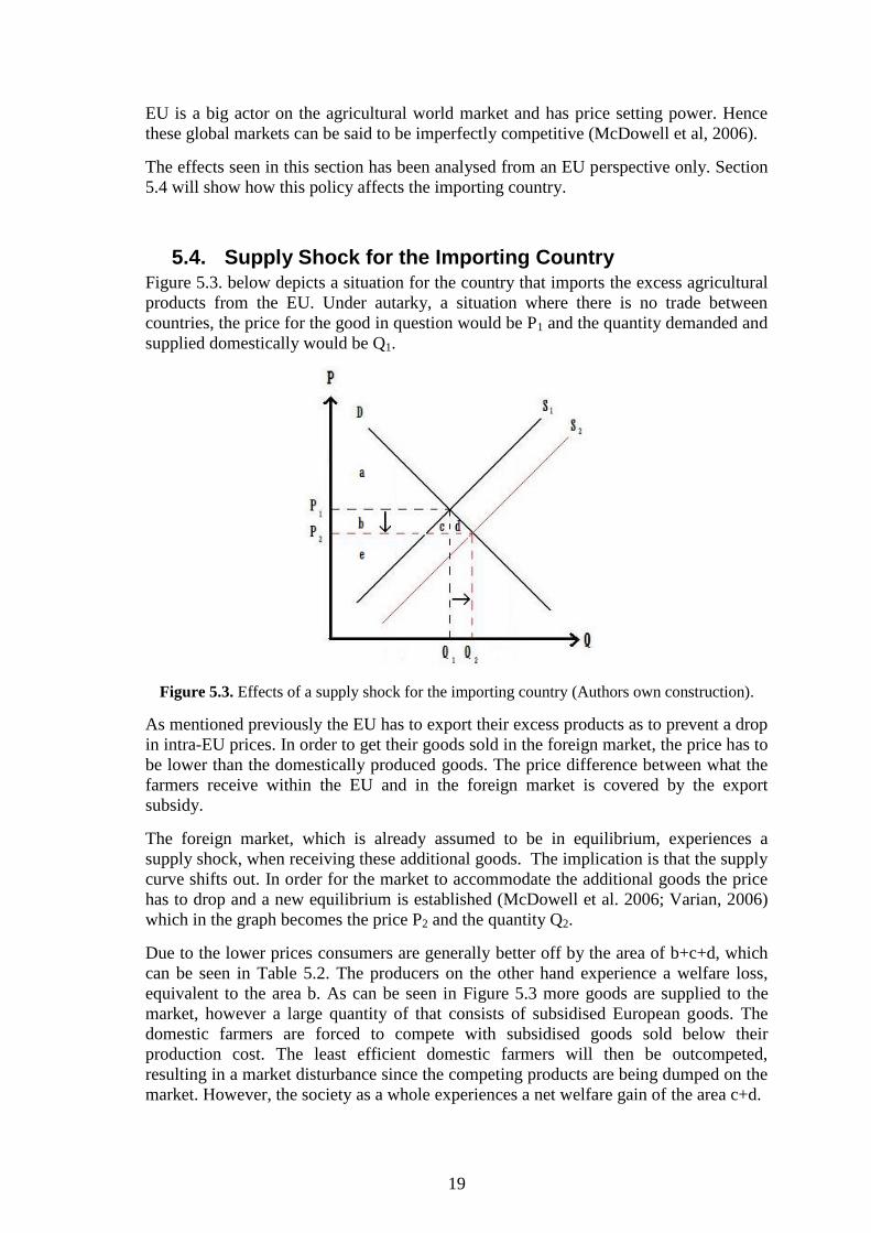
5.4. Supply Shock for the Importing Country Figure 5.3. below depicts a situation for the country that imports the excess agricultural

products from the EU. Under autarky, a situation where there is no trade between

countries, the price for the good in question would be P1 and the quantity demanded and

supplied domestically would be Q1.

Figure 5.3. Effects of a supply shock for the importing country (Authors own construction).

As mentioned previously the EU has to export their excess products as to prevent a drop

in intra-EU prices. In order to get their goods sold in the foreign market, the price has to

be lower than the domestically produced goods. The price difference between what the

farmers receive within the EU and in the foreign market is covered by the export

subsidy.

The foreign market, which is already assumed to be in equilibrium, experiences a

supply shock, when receiving these additional goods. The implication is that the supply

curve shifts out. In order for the market to accommodate the additional goods the price

has to drop and a new equilibrium is established (McDowell et al. 2006; Varian, 2006)

which in the graph becomes the price P2 and the quantity Q2.

Due to the lower prices consumers are generally better off by the area of b+c+d, which

can be seen in Table 5.2. The producers on the other hand experience a welfare loss,

equivalent to the area b. As can be seen in Figure 5.3 more goods are supplied to the

market, however a large quantity of that consists of subsidised European goods. The

domestic farmers are forced to compete with subsidised goods sold below their

production cost. The least efficient domestic farmers will then be outcompeted,

resulting in a market disturbance since the competing products are being dumped on the

market. However, the society as a whole experiences a net welfare gain of the area c+d.

20

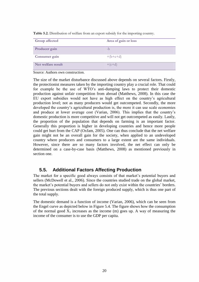
Table 5.2. Distribution of welfare from an export subsidy for the importing country.

Group affected Area of gain or loss

Producer gain -b

Consumer gain +(b+c+d)

Net welfare result +(c+d)

Source: Authors own construction.

The size of the market disturbance discussed above depends on several factors. Firstly,

the protectionist measures taken by the importing country play a crucial role. That could

for example be the use of WTO’s anti-dumping laws to protect their domestic

production against unfair competition from abroad (Matthews, 2008). In this case the

EU export subsidies would not have as high effect on the country’s agricultural

production level; not as many producers would get outcompeted. Secondly, the more

developed the country’s agricultural production is, the more it can use scale economies

and produce at lower average cost (Varian, 2006). This implies that the country’s

domestic production is more competitive and will not get outcompeted as easily. Lastly,

the proportion of the population that depends on farming is an important factor.

Generally this proportion is higher in developing countries and hence more people

could get hurt from the CAP (Oxfam, 2005). One can thus conclude that the net welfare

gain might not be an overall gain for the society, when applied to an undeveloped

country where producers and consumers to a large extent are the same individuals.

However, since there are so many factors involved, the net effect can only be

determined on a case-by-case basis (Matthews, 2008) as mentioned previously in

section one.

5.5. Additional Factors Affecting Production The market for a specific good always consists of that market’s potential buyers and

sellers (McDowell et al., 2006). Since the countries studied trade on the global market,

the market’s potential buyers and sellers do not only exist within the countries’ borders.

The previous sections dealt with the foreign produced supply, which is thus one part of

the total supply.

The domestic demand is a function of income (Varian, 2006), which can be seen from

the Engel curve as depicted below in Figure 5.4. The figure shows how the consumption

of the normal good X1 increases as the income (m) goes up. A way of measuring the

income of the consumer is to use the GDP per capita.

21

Figure 5.4. Engel curve for a normal good (Authors own construction based on Varian, 2006).

The foreign demand can be measured by the amount of exports. Thirlwall (2002)

recognises the positive effect increased exports, i.e. increased foreign demand, have on

the long run growth of output. This in turn is positive for a country’s growth.

What have been covered so far are the actors that make up a market. However, there is

always a risk of disturbances and noise when it comes to the production and/or the

transportation of the good. One such factor the World Bank has recognised is natural

disasters (Parker, 2006). According to the World Bank; natural disasters affect the

economy negatively and developing countries are especially vulnerable. Floods and

droughts, for example, have negative effects on agricultural activities.

5.6. Summary The table below, Table 5.3., summarises the effects the variables discussed in section

five have on a developing country’s dairy production, as suggested by the economic

theories presented. These effects are the hypotheses tested in the thesis with the main

variable of interest being the import from the EU.

Table 5.3. Hypotheses

Variable Effect

Import from EU Negative

Import from other countries Negative

Export Positive

GDP per capita Positive

Natural disasters Negative

22

6. Empirical Section The section applies the theoretical framework on real world data. This is done in order

to draw conclusions regarding the hypothesised effects CAP policies are said to have on

the developing countries’ dairy production. In addition, the general assumptions made

in this study are outlined and described along with the method used.

6.1. Presentation of Model and Variables Initially the contemplated model contained six variables; imports from EU, imports

from the remaining countries, export, natural disasters, GDP and population. When

developing the model the first step was to look at how correlated the variables were in

order to avoid future multicollinearity problems. It was discovered that population and

GDP were highly correlated; instead of dropping one of the variables they were

combined into GDP per capita. Taking the natural logarithms of the variables was

considered useful in this model as it describes the marginal effects in percentages.

Hence, the final model looks like the following:

lnprod= α+ β1lnEUimp+ β2lnnonEUimp+β3lnexp+ β4ln GDPperCAP+ β5trend+ β6ND+

β7adj+ β8Jamaica+,...,+β29Sudan+ εi

Production (lnprod)

The dependent variable has been collected from the Food and Agriculture Organization

(FAO), which is a division of the United Nations. In their database FAOSTAT figures

of production were retrieved for ―cow milk, whole, fresh‖. The database reported the

figures in metric tonnes; however, they were transformed into kilograms. This was done

to facilitate the interpretation of this variable when looking at the descriptive statistics.

The FAO only reports the top 20 commodities produced by a country. The observation

for Belize in 1992 is therefore missing since the production that year was too small to

be in the top 20.

Imports from EU (lnEUimp)

This explanatory variable was collected from Comtrade, a database created and

maintained by the UN containing statistics on international trade. To find the

commodity of interest the SITC (Standard International Trade Classification) rev.1

classification was used. SITC was preferred over the other classification HS

(Harmonized System) due to more available data and revision 1 was used because it was

the only revision that covered the years of interest. The unit used in the database was

kilograms. In order to get a figure for the quantity of dairy products the subcategories

022(milk and cream), 023(butter) and 024(cheese and curd) had to be added together.

Aggregated figures for the EU were only available from the year 2000 and onwards,

hence for the previous years the figures for the individual member countries had to be

added together. Consideration was given to the enlargements of the EU7. The figures

taken were the export figures reported by the member countries.

Imports from non-EU countries (lnnonEUimp)

This explanatory variable was collected from Comtrade using SITC rev.1 categories

022,023 and 024 as previously explained for the imports from the EU variable. The

7 A list of member countries and when they joined the EU can be found in Appendix 3.

23

figures were calculated by taking the aggregated world imports as reported by each

country and subtract the aggregate EU exports. The unit used was kilograms.

Exports (lnexp)

This explanatory variable was collected from Comtrade using SITC rev.1 categories

022,023 and 024 as previously explained for the imports from EU variable. It was

retrieved by taking each country’s reported export to the world. The unit used was

kilograms. When an export value was missing the assumption made was that no exports

occurred. However, a natural logarithm cannot be taken on a value of zero; hence it was

replaced by the value 1.

GDP per Capita (lnGDPperCAP)

This explanatory variable has been calculated by combining the two variables GDP and

population, i.e. GDP divided by population. The data for GDP was collected from the

UNdata and is stated in constant 1990 USD. The population was collected from the

database Gapminder.

Trend (Trend)

Some data showed clear trends over time. In order to adjust for this, a trend variable was

included that ranges from 1 for the first year to 31 for the last.

Natural disasters (ND)

The dummy variable was comprised by collecting data for various kinds of natural

disasters and combining them into one. The database used was The International

Disaster Database (EM-DAT) and the types of disasters included were; drought, flood,

storm and earthquake. A value of 0 means that there were no natural disasters reported

for that year, whilst 1 means that at least one natural disaster of one of these four types

did occur.

Adjustment (adj)

The dummy exists to adjust for the missing values of exports. The number 0 indicates

that no modification was made; the country reported a non-zero export. The number 1

indicates that no export was reported.

Country dummies (Jamaica,....,Sudan)

The country dummies are incorporated in the model to allow for each country’s

intercept to vary due to differences between the countries’ domestic production levels.

Error term (ε)

The error term is added to the model in order to capture the effects from the omitted

variables and possible misspecifications.

6.2. Additional Assumptions Except for each variable’s specific assumptions outlined previously, there are some

additional assumptions that need to be presented.

The assumption made about the dairy products imported from the EU is that all dairy

products have been subsidised in at least one stage. Either the good received subsidies

during its production, during its export or during both stages.

24

Two different databases have been used to collect information about dairy products. The

assumption made was that category 022,023 and 024 as reported in Comtrade

correspond to the production of ―cow milk, whole, fresh‖ as reported by FAO. This

assumption is made since the milk produced can be used in the production of butter

and/or cheese, which is not reported by FAO.

When determining which countries to use in the dataset Africa, South- and Central

America were investigated. The criterion for including a specific country was a

maximum of 5 missing observations for South- and Central America and 7 missing

observations for Africa. This differential treatment is due to less reported data from the

African countries.

For some years Comtrade only reported the value of the exports/imports instead of both

the quantity and value as normally done. The quantity was then received by calculating

the price per kg for two years preceding the missing value and two years succeeding the

value. An average was calculated and the value given by Comtrade was divided by the

estimated average in order to receive an estimated quantity. This has only been

necessary in a few cases and is not expected to have an impact on the result.

When calculating the non-EU imports some years became negative due to reported

errors by the countries. This would imply that more than 100% of the imports came

from the EU which results in two problems; firstly the value cannot exceed 100% out of

pure logic and secondly one cannot take the natural logarithm of a negative value. At

the occasions when the value exceeded 100% the value was modified to 99.9999%,

implying that almost all the imports were assumed to come from the EU. In addition,

the non-EU imports become a positive number, albeit small. This is not assumed to

affect the results of the regression.

6.3. Econometric Method To estimate the production regression function, the ordinary least square (OLS) method

was used. In order to be more efficient with the degrees of freedom, the data was

compiled into a pooled data set where the least-squares dummy variables model

(LSDV) was used. The method implies that each country, except from one, is given a

specific dummy variable that will take into account each country’s individual conditions

by allowing their intercept to differ. However, the regressors’ slope coefficients are

assumed to be the same (Gujarati, 2003). By using this method, a generalised result of

the data can be received which leaves out the task of individual country-case studies.

The base country, the country referred to when all country dummies are zero, is Brazil.

The results of these dummies are not presented in the regression output but can be found

in Appendix 6.

Due to the large amount of dummy variables included in the model heteroscedasticity

was present. In order to correct for this, robust standard errors were computed instead of

the ordinary standard errors (Gujarati, 2003).

A trend variable was included in the regression to deal with any trends in the data. The

trend caused by lnGDPperCAP on the lnproduction variable is thus explained by the

new trend variable and the remaining explanatory variables thus explain the variances in

production not caused by time (Gujarati, 2003).

25

6.4. Descriptive Statistics of the Model Variables As shown in Table 6.1 the countries in this study, on average, import more than they

export. This can be seen by looking at the mean value for lnexp which is lower than the

aggregated value for lnEUimp and lnnonEUimp, which constitutes the import from the

whole world8. This suggests that the countries in question do not have a production that

is sufficient for their own consumption needs. Their relatively low export also suggests

that they may not be competitive enough to compete on the world market. In addition,

the dummy variable adj has a mean value of approximately 0.175. This indicates that in

17.5% of the cases, no export at all of dairy products was reported from the countries in

the study to the world. This translates to approximately every 5th

year.

When considering the lnprod variable, conclusions regarding changes in the production

level are difficult to make. This is because this is a pooled data set containing the

production level of 23 countries during a time span of 31 years. The difference between

the minimum and maximum values could be due to both country differences and to

changes over the years.

Table 6.1. Descriptive statistics

Variable Minimum Maximum Mean Std. Deviation

No. of obs.

Lnprod 13.89 23.96 20,04 1.82 712

lnEUimp 4.61 19.14 15.10 1.74 708

lnnonEUimp -7.509 20.50 14.68 4.55 684

Lnexp 0 19.43 10.87 5.67 713

ln GDPperCAP 5.33 8.78 7.22 0.70 713

Trend 1 31 16 8.95 713

ND 0 1 0.55 0.50 713

adj 0 1 0.18 0.38 713

The ln GDPperCAP in Table 6.1. has a fairly low standard deviation which could be

due to several reasons. One reason might be that there has been a slow welfare

development in these countries over time. The low standard deviation could also

indicate that these countries are fairly similar economically, when it comes to their GDP

per capita variations.

8 The reader should be aware of that the import and export figures in the Table 6.1., may also be between

the countries in the study. However, the intra trade is not assumed to have any impact on the conclusions

drawn.

9 When the original value is between 0 and 1 the natural logarithm is negative.

26

It is also interesting to notice that the mean of the ND dummy exceeds 0.5. This

suggests that it is more common in these countries to experience a natural disaster than

not.

6.5. Output of the Regression Model Looking at the regression output in Table 6.2., one can see that the constant is positive

and significant on the 1% level. The positive value suggests that there will always be a

production of dairy products.

The main variable lnEUimp received a negative value of –0.034 and is significant on

the 1% level. The interpretation of this is that a 1% increase in the imports from EU to

the countries in the study will decrease their own dairy production with 0.034%. The

negative impact of the EU imports on the countries’ own production of this commodity

is in line with the hypothesis.

The variable lnnonEUimp has a value of 0.005 and hence affects the dairy production

positively. This is in contrast to the EU import and not in line with what one could

expect. The coefficient is significant on the 10% level.

Table 6.2. Regression output

Variable B t-statistic

Constant 21.608*** 26.03

lnEUimp -0.034*** -3.35

lnnonEUimp 0.005* 1.74

Lnexp 0.025*** 4.68

ln GDPperCAP 0.203* 1.87

Trend 0.019*** 9.58

ND -0.006 -0.25

Adj 0.115 1.45

R2 0.974

N 681

Notes: ***=significant on the 1% level, **=significant on the 5% level and *=significant on the 10% level.

The lnexp variable has a positive value of 0.025 and is significant on the 1% level. This

implies that when exports of dairy products increase with 1%, the production level of

that commodity increase with 0.025%. This is in line with the theoretical expectations.

A similar result can be seen from the ln GDPperCAP variable. Its coefficient value also

affects the production positively with an increase of 1% in the GDP/capita resulting in

an increase in the production of 0.203%. Thus, this variable has the largest impact on

the dairy production for these countries.

27

The trend variable has a positive coefficient which indicates a positive trend in the

production level. Looking at the dummy variables, the ND dummy has a negative value

indicating that a natural disaster would cause the production to decrease, which is in line

with the hypothesis in section 5.6. However, the low t-statistic indicates that this

dummy is not significant which would imply that natural disasters do not have any

impact on the dairy production level for these countries. The second dummy variable

show that the years when no export occurs, the intercept would have to increase with

0.115 units. However, this dummy is not significantly different from zero either, which

states that the adjustments made in the data set not is proven to have an impact on the

result of the regression.

The R2

indicates the goodness of fit of the model. The value of 0.974 indicates that

97.4% of all variation in the production level is explained by the explanatory variables.

The regression output also contains an additional 22 dummy variables which all are

significant on the 1% level; more details can be found in the Appendix 6.

6.6. Analysis As can be seen from the empirical results, the EU’s exports do effect the dairy

production in the countries studied negatively; when the imports from the EU increase

with 1% the dairy production in these developing countries will decrease with 0.034%.

This confirms the theory outlined in section five and confirms that EU’s subsidised

export is market distorting for the developing countries’ domestic dairy production. Due

to its negative effects, without the EU dumping its dairy products on their markets, the

domestic production could be assumed to increase. As explained by Rostow (1960) and

Balassa (1977), agricultural production is important for a countries development in the

initial stages. Due to that the development in the agricultural sector is considered to

stimulate further development in other areas, one could assume that the EU is slowing

down the development for undeveloped countries. This is not in line with the

development promoting objectives the EU has stated in article 177 of the EC treaty.

The study also found, by looking at the descriptive statistics, that these developing

countries are net importers of dairy products. This suggests that they do not have a

comparative advantage in dairy production, but the EU might have due to being such a

large exporter of these commodities. However, the theory section showed how domestic

support encouraged overproduction, which was found to be the case within the EU by

the study from Frandsen et al. (2003). Hence, reasons why the EU is such a larger

exporter of dairy products most likely comes from the domestic- and export subsidies

their farmers receive, rather than having a comparative advantage in the production of

dairy products.

By being net importers of dairy products, the developing countries in the study are

assumed to benefit from the CAP, which can be seen from Table 5.2. This is due to the

cheaper food prices created by the EU’s policy, which also is a general consensus in

previous literature (Matthews, 2008; Bouët et al., 2005). However, the countries in the

study are in general undeveloped, or have been during the time period examined. This

implies that the farmers do not have many other work opportunities when outcompeted

by subsidised EU products, as highlighted in the reports by Oxfam (2005) and Fokker

and Klukist (2000). Additionally, the thesis shows how the exports from the EU are

very fluctuating since what is exported is the excess supply only. This implies that a

28

developing country cannot rely on steady supplies of agricultural products from the EU.

Meanwhile, their own production is not given the opportunity to develop. It can thus be

concluded that the short run gains, from cheap food supplies, might be very costly in the

long run since their development might come to a halt. This might suggest why

developing countries, which often not have been able to use export- and domestic

subsides, lobbied for a specific agreement regulating the world trade of agricultural

products during the Uruguay Round. The regulated limits regarding export subsidies,

which were decided during the negotiations, has not been breached by the EU within its

dairy sector. However, even though having stayed within its allowed limits, the base

years chosen allowed for a continued high use of this type of subsidy. Hence, pressure

of further liberalising the agricultural trade has since then carried on from the

developing countries within the WTO. This has made the EU, under the ongoing Doha

Round, to consider removing its export subsidies by 2013.

The empirical result for the non-EU imports was the opposite of what was expected

from the hypothesis. However, the Table 6.1 shows that the variation in non-EU imports

is very large in comparison to the imports from EU; hence it might be more difficult to

measure a relationship between these imports and the domestic dairy production. In

addition, the EU imports are significant on the 1% level, whereas the non EU imports

are not significant until the 10% level, hence there is a larger risk of committing a type I

error in the latter case.

The variables lnexp and lnGDPperCAP both confirmed the hypotheses made regarding

their effects on production; both positively affected production in the countries studied.

The GDP per capita variable was found to have the highest impact on the dairy

production amongst all the variables studied. This could be due to the relatively low

change in the GDP per capita over the years and the relatively high change in

production. This would imply that a small, positive change in the GDP per capita results

in a relatively large increase of the production. The high impact, in comparison to the

export variable, also suggests that the domestic demand has a larger impact on

production than the foreign demand. Consider the relatively low quantity of exports

from the countries studied, this is not a surprising result.

Looking at the dummy variables, natural disasters showed the hypothesised sign but

proved to be insignificant. One reason for the insignificance could be that the natural

disasters occurred locally and did therefore not have a significant effect on the

production in the country as a whole. The dummies assigned to each specific country all

became significant and had a negative sign. This indicates that each country’s domestic

production were at a lower level when compared to the base country. The base country

used in the study was Brazil; the largest country in the sample. Hence, the negative

signs for the other countries were not surprising results.

On a whole, the model confirms the underlying theories used in this study. In addition,

the high R2 value indicates that the model developed for this study does explain a lot of

the variation in dairy production.

29

7. Conclusion The purpose of the thesis was to analyse the effects of EU’s subsidised dairy products

on the production in developing countries and to quantify these effects. The empirical

result showed that the subsidised imports from the EU distort the dairy production in

developing countries by the amount of 0.034% for every additional percentage increase

of import. This confirms the main hypothesis made in the study as well as answers the

purpose of the thesis. By stopping this behaviour of exporting subsidised goods, the

domestic production could be assumed to increase. Hence, the long run effects which

could come from this could be welfare enhancing for the countries in the study. Thus,

the thesis supports the study made by Diao et al. (2002).

The thesis found that the exports of dairy products from the EU most likely are a result

of the use of domestic- and export subsidies rather than the result of comparative

advantages. However, even though the use of these subsidies contributes to gains for net

importing developing countries in terms of cheaper food supplies the policies might be

very costly in the long run. This is due to the development gains that are expected to

come from an increased domestic production.

Due to the negative effects the imports from the EU showed to have on the developing

countries’ dairy production, the conclusion can be drawn that the EU is not policy

coherent with its development promoting objectives. However, over the years, CAP has

been reformed and under the ongoing Doha Round, the EU has made suggestions to

remove its export subsidies. This is seen as positive for the future prospects of

developing countries.

Another result found was that the domestic demand showed to have a larger effect on

production than the foreign demand. This is suggested by the relatively large coefficient

for the GDP per capita variable on production in comparison to the coefficient for the

export variable.

In general, most previous studies within this field have had their focus on the effects on

world prices of liberalising agricultural trade. The focus of this thesis has been on the

size of the distortion in domestic production caused by the EU’s subsidies. Hence the

conclusions of the thesis are therefore an important step towards being able to calculate

overall effects of such policies in future research studies. However, the findings of the

thesis support the previous studies made by, Oxfam (2005) and Fokker and Klukist

(2000) in that the EU outcompetes local farmers.

A suggestion for future research could be to examine the effect of dumping by using the

value of export- and domestic subsidies instead of the quantity exported, as done in this

study. Another suggestion for future studies could be to compare developing countries

that import subsidised goods versus countries that import non-subsidised goods to see

whether the effects on their domestic production differ.

30

List of references

Aczel, A. D. and Sounderpandian, J. (2006). Complete Business Statistics (6th

ed.). New

York: McGraw-Hill Education.

Agebjörn, A., (2007). Utveckling på Export?: EU: s Handelsavtal med Afrika och

Latinamerika. Globala Studier Nr. 29.

Altomonte, C. and Nava, M. (2005). Economics and Policies of an Enlarged Europe.

Cheltenham: Edward Elgar.

Andreosso-O’callaghan, B. (2003). The Economics of European Agriculture.

Basingstoke: Palgrave MacMillan.

Balassa, B. (1977). A ‖Stages‖ Approach to Comparative Advantage. World Bank Staff

Working Paper No. 256.

Bouët, A., Bureau, J. C., Decreux, Y., and Jean, S. (2005). Multilateral Agricultural

Trade Liberalization: The Contrasting Fortunes of Developing Countries in the Doha

Round. The World Economy, 28(9), pp. 1329–1354.

Bureau, J., Jean, S., and Matthews, A. (2006). The consequences of agricultural trade

liberalization for developing countries: distinguishing between genuine benefits and

false hopes. World Trade Review, 5(2), pp. 225-249.

Cardwell, M. (2004). The European Model of Agriculture. Oxford: Oxford University

Press.

Diao, X., Roe, T., and Somwaru, A. (2002). Developing Country Interests in

Agricultural Reforms under the World Trade Organization. American Journal of

Agricultural Economics, 84(3), pp. 782-790.

El-Agraa, A. M. (2004). The European Union: Economics & Policies (7th

ed.). London:

Financial Times Prentice Hall.

European Commission (2004). The Common Agricultural Policy Explained. Retrieved

December 3, 2009, from

http://www.fp7.org.tr/tubitak_content_files/268/komisyon_dokumanlari/cap_en.pdf

European Commission, (2009b). Economic Impact of the Abolition of the Milk Quota

Regime – Regional Analysis of the Milk Production in the EU. Retrieved January 17,

2010,from http://ec.europa.eu/agriculture/analysis/external/milkquota/full_report_en.pdf

European Commission (2010). How Much the CAP Costs. Retrieved January 14, 2010,

from http://ec.europa.eu/agriculture/capexplained/cost/index_en.htm.

EU (2006). European union — consolidated versions of the treaty on european union

and of the treaty establishing the european community. Retrieved January 13, 2010,

31

from http://eur-

lex.europa.eu/LexUriServ/LexUriServ.do?uri=OJ:C:2006:321E:0001:0331:EN:PDF

Fokker, R. and Klukist, J. (2000). EU: s Gemensamma Jordbrukspolitik – Bristen på

Samstämmighet. Globala Studier Nr. 1.

Frandsen, S. E., Gerfeldt, B., and Jensen, H. G. (2003). The Impacts of Redesigning

European Agricultural Support. Review of Urban and Regional Development Studies,

15, (2), pp. 106–31.

Grasser, H., (2005). We Feed the World [Motion picture]. United States: Bullfrog Films

Gujarati, D. N. (2003). Basic Econometrics (4th

ed.). Singapore: McGraw-Hill

Education.

Krugman, P. R. and Obstfeld, M. (2006). International Economics: Theory & Policy

(7th

ed.). Boston: Addison & Wesley.

Matthews, A. (2008). The European Union’s Common Agricultural Policy and

Developing Countries: the Struggle for Coherence. Journal of European Integration,

30(3), pp. 381-399.

McCulloch, J. R. (1888). The works of David Ricardo. London: John Murray

McDowell, M., Thom, R., Frank, R. and Bernanke, B. (2006). Principles of Economics.

London: McGraw-Hill Education.

McMillan, M. S., Peterson Zwane, A., and Ashraf, N. (2007). My Policies or Yours:

Does OECD Support for Agriculture Increase Poverty in Developing Countries? In A.

Harrison (Ed.), Globalization and Poverty (p. 183- 240). Chicago: University of

Chicago Press.

Oxfam. (2005), A round for free. How Rich Countries are Getting a Free Ride on

Agricultural Subsidies. Oxfam, United Kingdom.

Parker, R.S. (2006). Hazards of Nature, Risks to Development: An IEG Evaluation of

World Bank Assistance for Natural Disasters. The World Bank.

Piccinini, A., Loseby, M. (2001). Agricultural Policies in Europe and the USA:

Farmers between Subsidies and the Market. Basingstoke: Palgrave.

Rostow, W. W. (1960). The stages of Economic Growth: A non-communist Manifesto.

London: Cambridge University Press.

Sarris, A. (2001). The Role of Agriculture in Economic Development and Poverty

Reduction: An Empericaln and Conceptual Foundation. World Bank Rural Development

Strategy Background Paper No. 2.

32

Seth, T., (2004). WTO och den Internationella Handelsordningen. Lund:

Studentlitteratur.

SVT, (2009). Glåpord och Ägg haglade i Bryssel. October 5, 2009, from

http://svt.se/2.22620/1.1716166/glapord_och_agg_haglade_i_bryssel

Thirlwall, A. P. (2002). The Nature of Economic Growth: An Alternative Framework

for Understanding the Performance of Nations. Cheltenham: Edward Elgar Publishing

Limited.

Varian, H. R. (2006). Intermediate Micro Economics: A Modern Approach (7th

ed.).

London: W.W. Norton & Company.

WTO, (2008). Understanding the WTO. Genève: World Trade Organization.

WTO, (2009). Members’ Participation in the Normal Growth of World Trade in

Agricultural Products – Article 18.5 of the Agreement on Agriculture. Committee on

Agriculte G/AG/W/32/Rev.11.

Correspondence

European Commission, (2009a). DG Agriculture and Rural Development (AGRI-

INFO@ec.europa.eu). Data on CAP expenditure. Received on December 7, 2009.

33

Appendix 1

Articles 177 and 178 of the EC treaty.

‖Article 177

1. Community policy in the sphere of development cooperation, which shall be

complementary to the policies pursued by the Member States, shall foster:

— the sustainable economic and social development of the developing countries, and

more particularly the most disadvantaged among them,

— the smooth and gradual integration of the developing countries into the world

economy,

— the campaign against poverty in the developing countries.

2. Community policy in this area shall contribute to the general objective of developing

and consolidating democracy and the rule of law, and to that of respecting human

rights and fundamental freedoms.

3. The Community and the Member States shall comply with the commitments and take

account of the objectives they have approved in the context of the United Nations and

other competent international organisations.

Article 178

The Community shall take account of the objectives referred to in Article 177 in the

policies that it implements which are likely to affect developing countries.‖

European union — consolidated versions of the treaty on European Union and of the

treaty establishing the European community (EU, 2006, p.126)

34

Appendix 2

Countries in the study

Algeria

Argentina

Belize

Bolivia

Brazil

Chile

Colombia

Costa Rica

Ecuador

El Salvador

Guatemala

Honduras

Jamaica

Kenya

Madagascar

Morocco

Nicaragua

Panama

Paraguay

Peru

Senegal

Sudan

Venezuela

35

Appendix 3

EU members, until 2005, and years of entrance

Year Country

1952 Belgium

Netherlands

Luxembourg

France

West Germany

Italy

1973 Denmark

Ireland

United Kingdom

1981 Greece

1986 Spain

Portugal

1990 East Germany

1995 Austria

Sweden

Finland

2004 Estonia

Latvia

Lithuania

Poland

Czech Republic

Slovakia

Hungary

Slovenia

Cyprus

Malta

36

Appendix 4

Three countries’ import of dairy products from the EU.

(Authors own construction, based on data from Comtrade)

These three countries were selected by a systematic sampling method. This means that every kth observation is chosen for investigation (Aczel & Sounderpandian, 2006). In this case the k was equal to 7 and they were picked from the order they appear in the data set compiled for this investigation.

0

2,5

5

7,5

10

12,5

15

17,5

20

22,5

25

27,5

30

Mill

ion

s o

f ki

logr

ams

Chile

Nicaragua

Madagascar

37

Appendix 5

Export subsidies in the EU given to dairy products.

(Authors own construction based on data from WTO)

A graph showing the export subsidies EU is allowed to have in comparison to how

much of it actually is used.

0

500

1000

1500

2000

2500

19

95

19

96

19

97

19

98

19

99

20

00

20

01

20

02

20

03

20

04

20

05

Me

tric

to

nn

es

Quntity of subsidised EU exports

Allowed subsidised quantity by the WTO

38

Appendix 6

Complete results from the regression.

Variable B Robust Std. Errors

T Sig. Lower Bound

Upper Bound

VIF

(Constant) 21.608 0.830 26.03 0.000 19.978 23.238

lnImpEU -0.034 0.010 -3.35 0.001 -0.054 -0.014 3.77

lnExport 0.025 0.005 4.68 0.000 0.015 0.036 7.67

lnNonEUimp 0.005 0.003 1.74 0.083 -0.001 0.011 1.49

lnGDP/capita 0.203 0.108 1.87 0.062 -0.010 0.415 24.63

Trend 0.019 0.002 9.58 0.000 0.015 0.023 1.56

Natural disasters

-0.006 0.024 -0.25 0.805 -0.054 0.042 1.24

dummy adjusted

0.115 0.079 1.45 0.148 -0.041 0.267 5.86

Jamaica -5.957 0.146 -40.86 0.000 -6.243 -5.671 2.84

Algeria -2.773 0.065 -42.70 0.000 -2.900 -2.645 2.60

Argentina -1.025 0.067 -15.20 0.000 -1.158 -0.893 2.89

Belize -8.447 0.159 -53.23 0.000 -8.758 -8.135 2.56

Bolivia -4.418 0.164 -26.99 0.000 -4.739 -4.096 6.30

Chile -2.324 0.032 -72.87 0.000 -2.387 -2.262 2.05

Colombia -1.234 0.085 -14.56 0.000 -1.400 -1.068 3.07

Costa Rica -3.534 0.046 -76.19 0.000 -3.625 -3.443 2.48

Ecuador -1.973 0.132 -14.94 0.000 -2.233 -1.714 4.71

El Salvador -3.665 0.118 -31.16 0.000 -3.896 -3.434 4.63

Guatemala -3.790 0.137 -27.64 0.000 -4.060 -3.521 5.46

Honduras -3.422 0.152 -22.57 0.000 -3.720 -3.124 6.25

Nicaragua -3.841 0.158 -24.27 0.000 -4.151 -3.530 5.01

Panama -4.826 0.036 -134.19 0.000 -4.897 -4.756 2.07

Paraguay -3.883 0.142 -27.30 0.000 -4.163 -3.604 5.91

Peru -2.633 0.081 -32.32 0.000 -2.793 -2.473 2.86

Venezuela -2.202 0.056 -39.22 0.000 -2.312 -2.092 2.17

Morocco -2.553 0.117 -21.85 0.000 -2.782 -2.323 4.48

Kenya -1.842 0.215 -8.55 0.000 -2.265 -1.419 10.15

Madagascar -2.896 0.264 -10.98 0.000 -3.414 -2.378 13.96

39

Senegal -4.820 0.156 -30.82 0.000 -5.127 -4.513 5.16

Sudan -1.424 0.180 -7.92 0.000 -1.777 -1.072 5.22

The confidence interval is made on the 95% level.