THE EFFECTS OF EDUCATION, INCOME, AND CHILD MORTALITY ON

FERTILITY IN SOUTH AFRICA

Kristin Dust

Bachelor of Arts (Women's Studies), University of Victoria, 2002 Bachelor of Science (Economics), University of Victoria, 2003

PROJECT SUBMITTED IN PARTIAL FULFILLMENT OF THE REQUIREMENTS FOR THE DEGREE OF

MASTER OF ARTS

In the Department of Economics

O Kristin Dust 2005

SIMON FRASER UNIVERSITY

Fall 2005

All rights reserved. This work may not be reproduced in whole or in part, by photocopy

or other means, without permission of the author.

APPROVAL

Name: Kristin Dust

Degree: M. A. (Economics)

Title of Project : The Effects Of Education, Income, And Child Mortality On Fertility In South Africa

Examining Committee:

Chair: Ken Kasa

Jane Priesen Senior Supervisor

Alexander Karaivanov Supervisor

Simon Woodcock Internal Examiner

Date Approved: Thursday, December 1,2005

. . 11

DECLARATION OF PARTIAL COPYRIGHT LICENCE

The author, whose copyright is declared on the title page of this work, has granted to Simon Fraser University the right to lend this thesis, project or extended essay to users of the Simon Fraser University Library, and to make partial or single copies only for such users or in response to a request from the library of any other university, or other educational institution, on its own behalf or for one of its users.

The author has further granted permission to Simon Fraser University to keep or make a digital copy for use in its circulating collection, and, without changing the content, to translate the thesislproject or extended essays, if technically possible, to any medium or format for the purpose of preservation of the digital work.

The author has further agreed that permission for multiple copying of this work for scholarly purposes may be granted by either the author or the Dean of Graduate Studies.

It is understood that copying or publication of this work for financial gain shall not be allowed without the author's written permission.

Permission for public performance, or limited permission for private scholarly use, of any multimedia materials forming part of this work, may have been granted by the author. This information may be found on the separately catalogued multimedia material and in the signed Partial Copyright Licence.

The original Partial Copyright Licence attesting to these terms, and signed by this author, may be found in the original bound copy of this work, retained in the Simon Fraser University Archive.

Simon Fraser University Library Burnaby, BC, Canada

Abstract

I analyze the effects of mothers7 education, household income, and child mortality

on completed fertility in South Ahca, using the 1993 South A h c a Integrated Household

Survey. I estimate an individual fertility choice model using an OLS, a 2SLS, and a

Poisson model. The 2SLS model accounts for the endogeneity of education, income, and

child mortality; and the Poisson model accounts for the fact that fertility is a non-negative

count variable. The point estimates are different enough between the three models to

suggest that fertility should be estimated with a model that accounts for both fertility

being a non-negative count variable and the explanatory variables being endogenous. My

results are broadly consistent with the literature on determinants of fertility rates in

developing countries.

Acknowledgements

I would like to thank my senior supervisor, Dr. Jane Friesen, for her invaluable

support, guidance, and encouragement through not only my project, but my entire

graduate programme.

I would also like to thank Alex Karaivanov for his generous advice, and Simon

Woodcock for his comments and suggestions.

Table of Contents

. . .............................................................................................. Approval. .ii

... .............................................................................................. Abstract. .m

............................................................................... Acknowledgements.. .iv

.................................................................................. Table of Contents.. .v

....................................................................................... List of Tables. .vi

.......................................................................................... Introduction.. 1

.................................................................. Section 1: Literature Discussion.. 4

Section 2: Theoretical Framework.. ............................................................... .8

.................................................................... Section 3: Estimation Model. . . lo

.................................................................................... Section 4: Data.. .I5

................................................................... Section 5: Estimation Method.. -16

................................................................................ Section 6: Results.. ..22

............................................................................ Section 7: Conclusions. .28

.......................................................................................... References. .30

List of Tables

Table 1 : Summary Statistics ....................................................................... 15

Table 2: Estimation for number of pregnancies with only positive number of

pregnancies. with fixed effects and robust standard errors ......................... 25

Introduction

High fertility rates in developing countries may be caused by the interaction of

many aspects of poverty: high child mortality rates, minimal education levels, low

incomes, lack of employment opportunities, the need for child labour, gender inequality,

and lack of financial security. Poverty is characterized by low levels of nutrition,

sanitation, and health care, which fosters the incidence of child mortality. High rates of

child mortality, in turn, may increase fertility rates because parents want to replace lost

children and insure against future losses. For low-income families, children can bring in

much needed resources, for example by collecting fuel wood and water1, or through

wages2. Lack of insurance and government provided old age security means parents must

rely on their children to care for them when they are old. If parents are risk averse, they

will desire more than a replacement number of children to ensure that enough will

survive to take care of them in old age. Gender inequality and cultural norms influence

fertility in three ways. First, boy-preference increases fertility when parents have a

preferred number of male children. Second, women often have disproportionately less

bargaining power in the household over fertility choices and contraceptive use. Third, in

countries where women face few education and employment opportunities, the

opportunity cost of their time is low, so the "price" of children is low, and parents will

choose to have more children.

While high fertility is the result of underdevelopment, it is also a cause. High

fertility rates pose a health risk to women and children, stretch already inadequate

infrastructure and limited resources at the community and household level, and create

1 Aggarwal, Netanyahu, and Romano (2001) ' Rammohan (2001); and Boldrin, De Nardi, and Jones (2005)

dependency burdens, in which the workforce is burdened by the need to support a large

population of children and adolescents. This means resources are spread out and there is

less investment per child, at both the government and the household level, in children's

health and education. As a result, literacy levels remain low and morbidity remains high

for the next generation, which in turn continues to experience high fertility rates. Low

levels of education, high morbidity, population pressure on resources, and gender

inequality are all pathways in the positive feedback system between high fertility and

underdevelopment. High fertility and child mortality levels constitute an equilibrium in

which many developing countries are trapped.

Econometric modeling of fertility choice must address two main problems: first,

since the dependent variable is a non-negative count variable, an OLS model will not

give the best fit because it may produce negative predicted values; and second, education,

income, and child mortality may all influence fertility, but will be correlated with

unobservable variables that also influence fertility. Both problems could result in

inconsistent coefficient estimate^.^

Fertility choice is highly correlated with unobservable individual characteristics

and socio-economic community variables that affect access to education, infrastructure,

and economic opportunities. South Africa provides an opportunity to try to control for

the unobservable socioeconomic variables because its history of racial discrimination and

apartheid government has created a socioeconomic environment clearly divided by

ethnicity. By using race, language, and religion as proxy variables for socioeconomic

conditions, much of the unobservable variation in fertility that is tied to education,

income and child mortality can be controlled for.

Wooldridge (2003)

South Africa has a colonial history that resulted in distinct divisions between its

citizens, based on race and ethnicity. There were four racial groups recognized by the

apartheid government: African, Coloured, Indian, and White. Before and during the

apartheid era, Africans were largely confined to one of ten small reserves, or homelands,

which were formed around chiefdoms. Coloureds originated out of the mixing of

Africans and the white settlers; they were given a higher social status than Africans and

formed their own cultural group concentrated mainly in the Cape province. Indians first

arrived as indentured labourers, and have since kept to urban areas. Whites are divided

into the original Dutch settlers, the Afrikaners; and descendents of English settlers.

This paper analyzes some of the determinants of fertility rates in South Africa,

using 1993 household level data. In particular, I estimate the effects of mothers'

education, income, and child mortality on completed fertility. Section 1 is a literature

review; section 2 lays out the theoretical framework; section 3 outlines the estimation

model; section 4 describes the data and gives summary statistics; section 5 specifies the

estimation method; section 6 details the results; and section 7 concludes.

Section 1 : Literature Discussion

Evidence of the significant effect of maternal education on fertility is extensive:

see Breierova and Duflo (2004), Handa (2000), Kim (2004), and Singh (1994). Maternal

education influences fertility though the opportunity cost of having children, the

incidence of child mortality, intrahousehold bargaining power, income, and information

processing.

Breierova and Duflo (2004) deal with the identification problem with mother's

education by constructing instrumental variables for parental education in Indonesia.

They are able to do this by taking advantage of an extensive school construction program

that occurred in the 1970s. Data on parents' schooling, region of birth, and school

construction locations allowed for estimates of parents schooling. They find that paternal

and maternal education affect child mortality rates equally and significantly, but that

maternal education matters more for reducing early fertility and increasing age at

marriage. In a 2SLS model they find that each year of education reduces total number of

children ever born by about 0.1.

Handa explores the effects of education on preferences for children and on the

opportunity cost of mothers' time in Jamaica. He compares the effects of maternal

education in rural areas to urban areas, where there are more employment opportunities.

Using a two stage least squares model to instrument for household expenditure and child

mortality, he finds that the effect of secondary education on reducing fertility is much

stronger in urban areas, even though desired number of children is the same in both areas.

His estimates for the elasticity of fertility with respect to income are -0.10 for urban

woman and -0.15 for rural women. For the elasticity of fertility with respect to education,

his estimates are -0.86 for urban women and-0.45 for rural women. His estimate for the

fertility replacement response is close to 1, which could be expected in a country such as

Jamaica where child mortality is low and parents may only respond to experienced child

mortality rather than expected child mortality.

The relationship between fertility and child mortality is complex. Bhalotra and

Soest (2005) focus on the biological relationship between fertility and child mortality in

India. The neonatal death of a child shortens the interval until the next birth, because

parents want to quickly replace the lost child andlor because of shortened post-partum

amenorrhea. In turn, the risk of mortality for the next child increases, whether because

the mother has not had time to physiologically or psychologically recuperate, or because

the risk of child mortality increases with a mother's total number of births. The authors

use a dynamic panel data model that follows women and their children in India through

the women's complete fertility history and allows for control of household heterogeneity.

They find that a neonatal death shortens the interval until the next birth by twenty per

cent and increases the probability of a subsequent neonatal death by five per cent.

In a cross section analysis of developing countries, Singh tries to identify the

impact of women's human capital, use of contraception, and labour force participation on

fertility rates. He finds that contraceptive use has a stronger impact on fertility than

either labour force participation or education, although the effect of education becomes

stronger when contraceptive use is left out of the regression equation. He suggests this

means that education may influence fertility primarily through the use of contraceptives.

This is consistent with Kim's study of the effect of women's education on birth spacing.

Kim uses data from Indonesia to show that 77% of the change in the effect of education

on fertility from 1974 to 1990 can be explained by implementation of family planning

programs. Kim concludes that maternal education works primarily through increasing

women's ability to process information about contraceptive use.

Benefo and Schultz, in their 1994 study of the determinants of fertility and child

mortality in Ghana and Cote d'Ivoire, find that household expenditures and child

mortality do not pass the Hausman test for exogeneity. Therefore, they use a two stage

least squares model to instrument for household expenditures and child mortality. For

child mortality they use variables reflecting access to safe water and health care facilities;

and for expenditure they use type of dwelling and material used on outside of dwelling.

They find that, when mortality rates are not instrumented for, if the rate of child mortality

doubles, a woman's fertility will increase by 0.09 in Ghana and 0.18 in Cote d'Ivoire.

When child mortality is instrumented for, then the replacement response in both countries

doubles; although, it changes sign in Cote d'Ivoire. For education, they find that

additional years of schooling beyond primary school are associated with reduced fertility,

although the estimates are not significant. Their coefficient estimates for the effects of

each year of primary, secondary, and post secondary school on number of births are -0.05,

-0.29, and -0.36 in Cote d71voire; and -0.02, -0.15, and -0.1 1 in Ghana. They find that

expenditures, without being instrumented, are insignificantly correlated with fertility in

either country; but significant at the 10% level when instrumented. For Ghana the sign

for the income coefficient is negative, while for Cote d'Ivoire it is positive.

Gangadharan and Maitra (2001) use the same data set as this paper to study

fertility patterns in South Africa. They estimate a Poisson model to analyze the effects of

income and education on fertility, both of which they treat as exogenous; and a 2SLS

model in which they include and instrument for child mortality. For the age group which

I am studying they find that both education and income are negatively correlated with

fertility. Their technique for instrumenting mortality is different fiom my study, in which

I regress individual mortality rates on household and community variables. Gangadharan

and Maitra regress mortality as a count variable on mortality rates and other exogenous

variables.

Section 2: Theoretical Framework

For the theoretical framework in this paper I will use a combination of Becker's

household economics model,4 the fertility model developed by Aggarwal et a15, and that

of Iyer and ~ e e k s . ~ In this model, households maximize utility, U, by choosing the

number of children, C, the quality of children, Q, and quantity of purchased goods, Xp, or

domestically produced goods, Xd. The utility function is constrained by a child quality

production function, a production function for domestic goods, constraints on household

income and mothers' time, and cultural expectations. The utility function is expressed as

follows:

Max U = U(C, Q, Xd, Xp)

Subject to: Child quality production function: Q = Q(Tq, Xp)

Tq = mother's time in child quality production function

Xp = purchased goods used in child quality production function

Domestic goods production function: Xd = X(Td, Xp)

Td = mother's time in domestic goods production function

Xp = purchased goods used for domestic goods production

Mother's time constraint: T = CTC + Tq + Td + TL

TC = time involved in child bearing

TL = time spent working in the labour market

Household income constraint: I = WTL + p Xd + R = pXp

w = wages from the labour market

Becker (1 98 1) 5 Aggarwal, Netanyahu, and Romano (2001) 6 Iyer and Weeks (2004)

p = price index for domestically produced and purchased goods

R = remittances from absent household members

Cultural expectations: E = E(ethnic group, community)

From this, a reduced form demand equation for children can be derived as a

function of prices, p; wages, w; income, I; and a preference parameter, a .

Ci" = c * (P, WY 1; a ) (1)

Let the preference parameter depend on mothers' individual characteristics, Xm;

household characteristics, Xh; community characteristics, Xc. The individual fertility

demand equation can then be described as

Ci" = C"(p, W, I; Xm, Xh, Xc) (2)

In this model, the fertility decision is assumed to be a choice made at the start of

the reproductive period. Parents' identify a desired number of surviving children, and

then choose an optimal number of pregnancies that takes into account expected child

mortality. In this paper I will estimate an empirical version of equation (2).

Section 3: Estimation Model

For this study I wish to focus on completed fertility, or the number of pregnancies

a woman has had over her entire reproductive period. The reason for using completed

fertility is that women will choose reproductive schedules to suit their individual needs.

Women who choose to stay in school longer, or need to stay at home to help their

mothers raise their younger siblings, may not choose to reduce their fertility. They may

instead choose to have children at a later age, but then have shorter birth intervals. If

there are younger women in the sample, I will not be able to isolate the effect of delayed

fertility from an age effect on total fertility choice.

Another reason for using completed fertility is that the women in the sample have

then had an opportunity to replace children who have died. There are two types of

fertility responses to child mortality: replacement and hoarding. The replacement effect

is an increase in fertility to compensate for experienced losses, while the hoarding effect

is an increase in the fertility choice, C*, at the beginning of the reproductive period by

risk averse parents who want to compensate for expected future 10sses.~ Since my

theoretical model assumes that expected losses are incorporated into the demand equation

for children, then any estimated changes in fertility in response to experienced child

mortality should be primarily a replacement effect. If there are younger women in the

sample who have not yet responded to child mortality, then I will not be able to

accurately estimate the effect of child mortality on fertility.

The most important of the mother's individual characteristics, Xm, being

examined is her education, which will be divided into primary school, high school, and

' Bhat (1998)

post secondary education. Education determines not only the opportunity cost of a

mother's time, but also her ability to access and process information pertaining to the

market or the household. Women who have more education may be better informed

about contraceptive use; and nutrition, medicine, and sanitation, which would affect

fertility through child mortality.8 Education is used as a proxy for the opportunity cost of

a mother's time when she chooses to raise a child rather than work for wages. Wages, for

which education proxies, are part of the cost or 'price' of children. A proxy for wages is

necessary in studies of developing countries, since most women do not participate in the

job market. For the sample used in this paper, only 6% of the women reported being in

the job market when the survey was taken.

Other characteristics of the mother that will be controlled for are age, age squared,

race, language, religion, and community cluster. Because I want to use completed

fertility as my dependent variable, I have restricted my sample to women aged forty-five

and older. The age and age squared variable should capture any remaining incomplete

fertility, as well as cohort effects from changes in socioeconomic and political conditions.

Language, race, religion, and community cluster are used to control for cultural and

community influences that may have a significant effect on preferences for family size.9

For example, mothers' expectations of child mortality, which will underlie the hoarding

effect, will be related to observations of local child mortality rates. Cultural

characteristics of ethnic groups may encourage or discourage female education and

labour market participation. By controlling for community and culture I am controlling

for observable and unobservable cultural and community influences on fertility that

Caldwell(1979) Iyer and Weeks (2004)

might be correlated with the explanatory variables. Community cluster variables will

control for observable community variables such as access to infrastructure and prices, p,

for inputs into the child quality and domestic goods production functions. These

variables may be observable, but fixed effects could control for them more thoroughly

than including what is available from the data.

The community cluster dummies will also control for access to contraceptives. If

contraceptive availability is affecting the number of times a woman is pregnant, then this

will be controlled for.

The reason both language and race are included in the estimation model is: first,

there is a significant difference in socioeconomic conditions within racial groups between

people who speak English or Afrikaans and those who speak their native language; and

second, there is a significant difference in socioeconomic conditions between ethnic

groups. Ethnicity is not measured by the survey, so language is used as a proxy. To

exemplify the effect of language in my sample, African households who speak their

native language have a mean income per member that is one eighth that of Afrikaans-

speaking African households and one twelfth that of English-speaking African

households. An example of ethnic differences within a racial group is the difference

between Afrikaners and English-speaking whites. The mean income per member for

Afrikaner households is two-thirds that of English-speaking whites, while the mean

education level is about one year higher for English-speaking white women than for

Afrikaner women in this sample.

For household characteristics, Xh, I will control for income per household

member1' and child mortality. Since the data reflects current household conditions,

rather than when the fertility decision was made, at the beginning of the reproductive

period, the income variable will be measured with error. However, I believe this will not

be a significant problem since current income would be closely correlated with past

income. Child mortality is considered a household characteristic because it is closely tied

to household conditions such as safety of the water supply, sanitation, and food quality.

For child mortality variables I will use mothers7 individual rates of stillborns, infant

mortality (deaths before the age of I), and child mortality (deaths between the ages of 1

and 5). The reason I use a mortality rate instead of a mortality count variable is that a

count variable will be positively correlated with fertility. A woman may have a higher

number of stillborns, infant, or child deaths simply because she has had more

pregnancies." Because the number of pregnancies is the denominator in the mortality

rate variables, these variables will also be simultaneously determined. They should,

however, be less endogenous than a mortality count variable.

Income has a somewhat ambiguous relationship with fertility. If children are

normal goods, then we would expect income and fertility to be positively correlated.

This is, however, almost never the case.12 Instead there appears to be a quantity-quality

trade-off, as theorized by Becker and ~ e w i s . ' ~ Income is an indicator of the opportunity

cost of parents7 time, so the higher the income, the higher the fixed opportunity cost of

having another child. Parents with higher incomes will substitute child quality for child

10 A per capita household equivalency scale may not be optimal since children use fewer resources than adults, but the only household composition variable available was household size. See Nelson (1993). I ' Benefo and Schultz (1 994) 12 Except in cases of extreme poverty, when mothers are too malnourished to carry pregnancies to term. l3 Becker and Lewis (1973)

quantity as income, or opportunity cost, increases, because the shadow price of an

additional child increases relative to the price of child quality inputs. For this reason we

would expect income to be negatively correlated with fertility.

Community characteristics, Xc, are controlled for by using a fixed effects model

organized by the community clusters, into which the households were grouped by the

survey. The fixed effects model will control for community variables, such as local food

prices, p; economic opportunities; child mortality expectations; cultural expectations; and

any other community influences on fertility preferences or the explanatory variables.

Fertility may be strongly correlated with socioeconomic conditions, since the

fertility choice will be affected by access to education, natural resources, infrastructure,

and employment opportunities. Education and employment opportunities determine the

opportunity cost of a woman's time, and will thus affect her utility maximizing fertility

choice. Access to natural resources may be negatively correlated with fertility if children

are needed as labourers to, for example, collect fuel wood.14 Access to infrastructure,

such as safe drinking water and health care will affect fertility through its effect on child

mortality'5. Unobservable socioeconomic variables will be correlated with mothers'

individual characteristics, Xm, household characteristics, Xh, and community

characteristics, Xc. Since culture and socio-economic conditions are so highly correlated

with ethnicity and race in South Ahca , controlling for race, language, and religion

should control for a significant amount of the variation in fertility that is due to socio-

economic conditions.

l4 Aggarwal, et a1 (2001) l5 Benefo and Shultz (1994)

Section 4: Data

The data used in this study is from the 1993 South A h c a Integrated Household

Survey. The purpose of the survey was to gain knowledge about the living environment

of South Africans in order to guide policy for the post-apartheid government. Nine

thousand households, divided into 360 clusters, were asked about income, expenditures,

employment, assets, education, health, and fertility. At the cluster level, data was

collected on local prices and access to health care facilities and natural resources.16

My sample consists of 858 women, aged 45 to 85, of which 63% are African, 9%

are Coloured, 5% are Indian, and 24% are White.

Table 1: Summary Statistics Mean Mean Mean Mean Mean

Variable (all) Min Max (Black) (Coloured) (Indian) (White)

Number of pregancies 4.45 0 14 5.04 4.29 3.23 3.00

Stillborn rate (%) 5.6% 0% 100% 4.8% 10.0% 2.9% 6.8%

Infant mortality rate 5.0% 0% 100% 6.6% 2.5% 3.0% 1.1%

(died before age 1)

Child mortality rate (died 3.2% 0% 100% 4.5% 2.0% 0% 0.4%

between 1 & 5)

Education (standards)I7 4.85 0 14 3.72 5.56 5.41 7.48

Total monthly income 704 0 21,058 262 530 754 2,129

per member (rands)"

l6 SALDRU 17 South African public education starts later and ends at standard 10; a university degree has a value of 14. 18 1 rand = $0.18 Cdn

Section 5: Estimation Method

There are two main identification problems when estimating the effects of

education, income, and child mortality on total fertility: censored data and endogenous

explanatory variables. Because of unobservable socioeconomic variables that affect both

fertility and the explanatory variables, ordinary least squares estimation will likely be

inconsistent. OLS could also result in negative predicted values for fertility, because it

does not account for the fact that fertility is a count variable that cannot take on negative

values.

A Poisson event count model is appropriate for modeling fertility because it

accounts for the nature of the dependent variable by using an exponential distribution.

The probability of Ni being n is a function of n and Xi, the expectation of ~ i ' ~ .

Pr (Ni = n) = e%? n !

However, since a Poisson distribution assumes equi-dispersion of the dependent

variable,20 over-dispersion will result in inefficient estimates, and the standard errors will

not be a reliable test of significance of the point estimate^.^' Using a likelihood ratio test

for significance of the dispersion yields an approximated chi-squared statistic

of 0.0006 with a p-value of 0.490. Over-dispersion is therefore not a significant problem

in the data, and a Poisson count model is appropriate.23

j9 Nguyen-Dmh ( 1 997) 20 Equi-dispersion occurs when the variance equals the mean; over-dispersion means the variance is greater than the mean. " Cameron (1990) 22 Wang and Famoye (1997) 23 See Wooldridge (2003), p 576 for how to adjust standard errors if there is significant over- or under- dispersion.

The second identification problem is potential endogeneity of the education,

income, and child mortality rate variables due to unobserved household characteristics.

Significant endogeneity will lead to inconsistent but efficient estimates because the error

term will be correlated with the explanatory variables.

Mothers have heterogeneous unobservable characteristics that affect both their

fertility and their education levels. Likewise, income may be influenced by the same

heterogeneous household characteristics that affect fertility. In South Ahca, these

unobservable characteristics that will influence fertility and be correlated with education

and income, could be ability and socioeconomic conditions. Women who have low

ability, and/or have constrained opportunities due to the apartheid social structure, may

be less likely to find wage labour. The low probability of finding employment lowers

their opportunity cost for having children; and consequently, their optimal fertility choice

may be higher. Income and education are also subject to the same time constraint that

binds the production of child quantity and quality. Women who go to school longer or

choose to participate in the labour market will have less time to bear and invest in

children. Other unobservable socio-economic variables, such as cultural and community

influences on fertility preferences, may be related to education through culturally defined

gender roles.24

The strong correlation between fertility and child mortality results from similar

input variables between the child health production function and the reduced form

demand equation for children. Hypotheses about the relationship are discussed in Bhat

(1998), Bholotra and Soest (2005), Frankenburg (1998), Handa (2000), and Rosenzweig

and Schultz (1983). Child mortality can be linked to fertility in two ways: first, short

24 Iyer and Weeks (2004)

birth intervals increase the chance of infant mortality;25 and second, high child mortality

rates lead to higher fertility because parents want to replace lost children andor insure

against future losses.26 These relationships may cause simultaneity bias as well as

omitted variable bias from unobservable household characteristics.

To deal with endogenous explanatory variables, I will use a two stage least

squares model with various household and community characteristics as instrumental

variables for education, income, and child mortality.

To instrument for child mortality, I will follow Aggarwal, et a127 and use a group

of household and community variables that will be correlated with child mortality but

uncorrelated with fertility. These variables are household water source (piped, internal;

piped, yard tap; water carrier; public tap, free; public tap, paid for; borehole; rainwater

tank; flowing river or stream; stagnant; well; or protected spring) or distance to the

nearest water source, and distance to the nearest nurse or doctor. Since many infant and

child deaths in developing countries are due to water bourn diseases, water source

variables should be highly correlated with infant and child mortality.

To instrument for income, I follow Benefo and ~ c h u l t z ~ ~ and used a group of

dummy variables for material used on outside of home (bricks, cement, pre-fab,

corrugated iron, wood, plastic, cardboard, mix of mud and cement, daub or wattle, mud,

thatching, or asbestos). Handa proposes that while building material is highly correlated

with income, it is less susceptible to measurement error and is a better indicator of long

run average income.

- - -

25 Bhalotra (2005) 26 Bhat (1998) 27 Aggarwal, et a1 (2001) 28 Benefo and Schultz (1 994)

To capture exogenous variation in education I have used province of residence as

an instrument. Province is correlated with the same socio-economic variables that affect

fertility; however, most of this correlation should be captured by controlling for language,

race, and religion. 29 There may be a problem if women have migrated between

completing school and when the survey was conducted; however, since migration was

severely restricted until the post-apartheid era I do not believe this will be a significant

problem. It was primarily men who were able to migrate because they had work permits.

Most of the women in my sample do not work now, and it is likely that most never have.

The potential source of exogenous variation in education that I am attempting to

capture with province has to do with the history of education and missionary presence in

South Africa. Western interest in missionary work grew rapidly around the turn of the

century due to the famous missionary explorer, David Livingstone; and a new emphasis

in Western Christianity on bringing the gospel to other countries. Missionary work in

Africa increased exponentially as different denominations competed for souls in the wake

of the European competition for land.30

In the first half of the twentieth century in South Africa, when most of the women

in my sample would have been going to school, education in the homelands was left

almost entirely to these mis~ionaries.~' The prevalence of schools would have been a

hnction of outside fimding for the missionaries, and how well the mission had integrated

into the community. How well a mission had integrated, in turn, would have been a

function of the hospitability of the climate32, relations with the local chiefs, level of

29 Thompson, Leonard (1995) 30 "African Christianity: a history of the Christian Church in Africa" 31 Thompson (1995) 32 Acemoglu and Robinson (200 1)

resistance to missionary teachings33, and past relationships between missionaries and

Ahcans.

For the dependent variable I chose number of pregnancies rather than number of

births because of inconsistencies in the data. For a small proportion of my sample,

stillborns were counted as pregnancies but not births. Since I calculate stillborn rate as

number of stillborns as a proportion of births, this would give me inaccurate calculations

for the stillborn rate. Using number of pregnancies, however, means that I will be

including pregnancies that ended in miscamage. My only option is to choose between

the two problems, since eliminating those observations altogether would lead to sample

selection bias. Examination of the data seems to show that stillborns not being counted

as births was more common than miscarriages, so I decided to use number of pregnancies

rather than number of births.

It would be ideal to use a model that could account for both the endogeneity of the

explanatory variables and the fact that the dependent variable is a non-negative count

variable. Options include generalized methods of moments or generalized empirical

likelihood models. See Boes (2004) for a discussion of the empirical likelihood method.

These procedures are not implemented in this paper.

Finally, I will use fixed effects to control for community variables that are

correlated with either fertility or the explanatory variables. By using fixed effects for

community clusters I will be controlling for any inter-cluster heterogeneity that may be

correlated with fertility through, for example, expectations of child mortality and

preferences for family size.

33 "Mission Settlements in South Africa"

For 65 of the 360 clusters, there is only one observation per cluster. To

compensate for the absence of a cluster effect estimate for those observations, I include

several price and infrastructure variables in the estimation model.

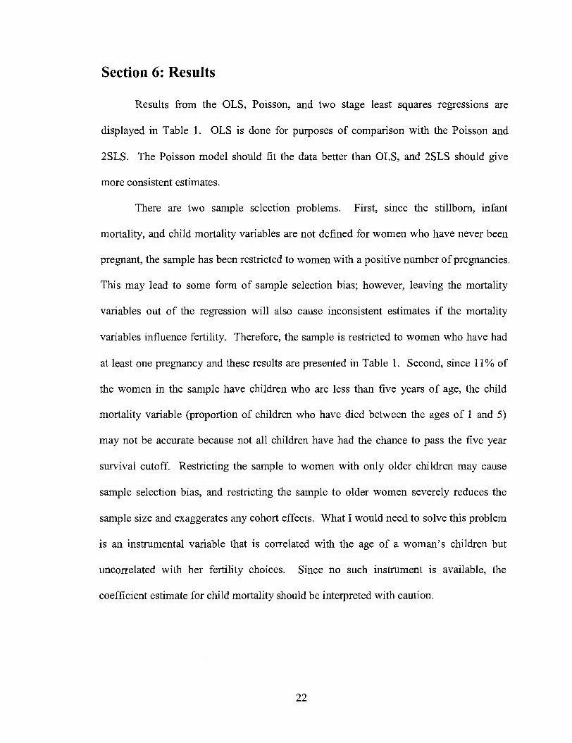
Section 6: Results

Results from the OLS, Poisson, and two stage least squares regressions are

displayed in Table 1. OLS is done for purposes of comparison with the Poisson and

2SLS. The Poisson model should fit the data better than OLS, and 2SLS should give

more consistent estimates.

There are two sample selection problems. First, since the stillborn, infant

mortality, and child mortality variables are not defined for women who have never been

pregnant, the sample has been restricted to women with a positive number of pregnancies.

This may lead to some form of sample selection bias; however, leaving the mortality

variables out of the regression will also cause inconsistent estimates if the mortality

variables influence fertility. Therefore, the sample is restricted to women who have had

at least one pregnancy and these results are presented in Table 1. Second, since 11% of

the women in the sample have children who are less than five years of age, the child

mortality variable (proportion of children who have died between the ages of 1 and 5)

may not be accurate because not all children have had the chance to pass the five year

survival cutoff. Restricting the sample to women with only older chldren may cause

sample selection bias, and restricting the sample to older women severely reduces the

sample size and exaggerates any cohort effects. What I would need to solve this problem

is an instrumental variable that is correlated with the age of a woman's children but

uncorrelated with her fertility choices. Since no such instrument is available, the

coefficient estimate for child mortality should be interpreted with caution.

For the two stage least squares estimation I followed the standard procedure34 by

first conducting auxiliary regressions for the three education levels, the three mortality

rates, and income on the instrumental variables and all other exogenous variables. I then

tested for endogeneity of education, income, and mortality by saving the residuals from

the auxiliary regressions and putting them back in the OLS~' and Poisson models36 to test

the degree to which they were correlated with the dependent variable, fertility. None of

the residuals are significant in the OLS model, but in the Poisson model high school

education and infant mortality are significant at the 5% and 10% levels, respectively.

The fact that the residuals are significant in the Poisson model, but not in the OLS model,

leads me to conclude that the education and mortality variables probably are endogenous,

but OLS does not fit the data well enough to identify their endogeniety. Since the

Poisson model does not account for endogeneity of the explanatory variables, the Poisson

estimates will not be consistent and should be interpreted carefully.

To test for exogeneity of my instruments for the 2SLS model, I did a test of

overidentifying restrictions for the hypothesis that at least some of the variables are

endogenous. The 2 test statistic is d = 32.95, which has a p-value of 0.778. This

allows me to conclude that my instruments are exogenous.37

The coefficient estimates are very similar between the OLS, the 2SLS, and the

Poisson regressions; however, more of the explanatory variables are significant with the

34 Wooldridge (2003), p.476 35 Wooldridge (2003), p.483 36 Wooldridge (1 997) 37 Testing for overidentifying restrictions can be done when there are multiple instrumental variables. The test statistic is I& and gauges the correlation between the 2SLS residuals and the exogenous variables. It follows a clu-squared distribution with q degrees of freedom, where q is the number of instrumental variables minus the number of endogenous variables. If the test statistic is small enough, then an insignificant amount of the residuals from the 2SLS structural equation is explained by the exogenous variables, and it cannot be concluded that some of the variables are endogenous.

Poisson model than with OLS. Conducting a two staged least squares regression using

these instruments yields insignificant estimates for all of the education, mortality, and

income variables, except for high school education which is significant at the 10% level.

This leads me to believe that either my instruments are too weakly correlated with the

explanatory variables to have significant explanatory power, or that my explanatory

variables do not significantly affect fertility.

The R2 values for my auxiliary regression are: 0.65 for primary schooling, 0.69

for high school education, 0.36 for post secondary education, 0.33 for stillborn rate, 0.45

for infant mortality rate, 0.47 for child mortality rate, and 0.82 for monthly income per

household member. These R2 values are fairly high for the auxiliary regressions, so the

insignificance of the instrumented explanatory variables is probably not due to weak

instruments. It is still interesting to compare the point estimates between the OLS and

2SLS models since, despite being less efficient, the 2SLS estimates should be more

consistent than the point estimates from the OLS or Poisson models.

With the OLS model, all of the education variables are negative, but none are

significant. Each year of primary school decreases number of pregnancies by 0.06; each

year of high school reduces pregnancies by 0.12; and each year of post secondary school

reduces pregnancies by 0.13. The magnitude of these coefficient estimates is consistent

with the literature for developing countries. The income elasticity of number of

pregnancies has an estimate of -0.33 and is significant at the 5% level. All of the

mortality variables are positively correlated with fertility, but none are significant. To

interpret these mortality rate estimates I will follow Benefo and Handa, and evaluate

them at the sample mean. A doubling of the stillborn rate is thus estimated to increase

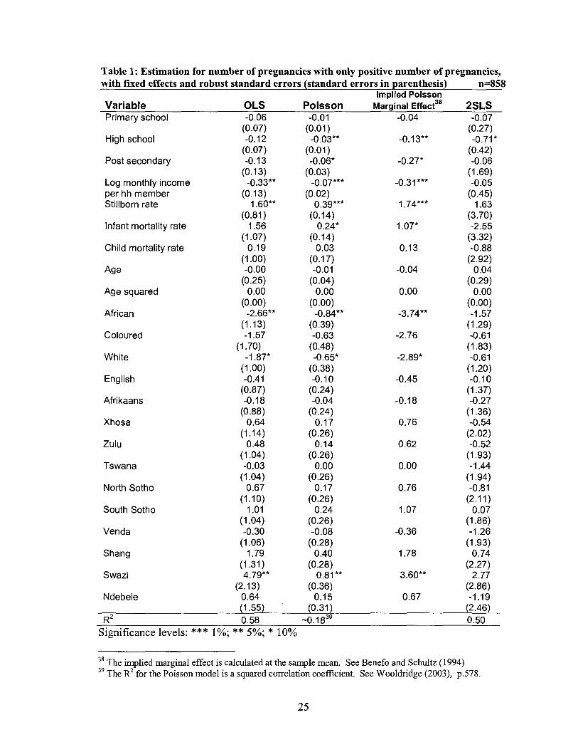
Table 1: Estimation for number of pregnancies with only positive number of pregnancies, with fixed effects and robust standard errors (standard errors in parenthesis) n=858

Implied Poisson Variable OLS Poisson Marginal ~ f f e c t ~ ' 2SLS Primary school

High school

Post secondary

Log monthly income per hh member Stillborn rate

Infant mortality rate

Child mortality rate

Age

Age squared

African

Coloured

White

English

Afrikaans

Xhosa

Zulu

Tswana

North Sotho

South Sotho

Venda

Shang

Swazi

Ndebele (1 55) (0.31) (2.46)

R~ 0.58 -0.18~' 0.50 Significance levels: *** 1%; ** 5%; * 10%

38 The implied marginal effect is calculated at the sample mean. See Benefo and Schultz (1994) 39 The R~ for the Poisson model is a squared correlation coefficient. See Wooldridge (2003), p.578.

fertility by 0.09; a doubling of the infant mortality rate increases fertility by 0.08; and a

doubling of the child mortality rate increases fertility by 0.01.

When instruments are used for education, income, and mortality in the 2SLS

model, only the high school variable is significant at the 10% level. The point estimates

for primary schooling are very similar between the OLS and 2SLS models, at -0.07 for

2SLS compared to -0.06 for OLS. For high school the ~ S L S estimate is about six times

higher than OLS, at -0.71 compared to -0.12. The post secondary school 2SLS estimate

is only half of that for OLS, at -0.06 compared to -0.13. The 2SLS estimate for log of

monthly income is much smaller at -0.05, compared to the OLS estimate of -0.33. For

mortality rates, the stillborn rate estimates are very close, at 1.63 for 2SLS compared to

1.60 for OLS. Both the infant and child mortality rates, however, become negative and

much larger in the 2SLS model. Interpreting these coefficient estimates as a response to

the doubling of the morality rates, the 2SLS response estimate for stillborn rate is 0.09,

for infant mortality is -0.13, and for child mortality the response is -0.04. This is

comparable to 0.09, 0.08, and 0.01 for the OLS estimated responses; but differs from

Gangadharan and Maitra (2001), who find in their study with this data set that all three

mortality variables are positively correlated with fertility. The magnitudes of the

mortality estimates are similar to those found by Benefo and Schultz, who also find that

the signs become negative with a 2SLS estimation method in the Cote d'Ivoire.

The 2SLS age estimates are comparable to the OLS estimates. All of the race

dummy estimates are the same sign but smaller in 2SLS than OLS. Most of the language

dummy estimates are similar in magnitude to the OLS estimates, although some of them

change signs.

In the Poisson model, both high school and post secondary education significantly

affect fertility. Every year of primary school reduces fertility by 1%; every year of high

school reduces fertility by 3%; and every year of post secondary school reduces fertility

by 6%. Evaluated at the mean fertility rate, these coefficients imply a reduction of 0.04,

0.13, and 0.27 children for each year of primary, secondary, and post secondary

schooling. Log of monthly income per household member is significant at the 1% level

and implies an income elasticity of demand for children of -0.3 1. All of the mortality

rates are positive, although only the stillborn and infant mortality rates are significant at

the 1% and 10% levels, respectively. Evaluated at the mean fertility and mortality rates,

the coefficient estimates imply that a doubling of the stillborn, infant, and child mortality

rates will increase fertility by 0.10, 0.05, and 0.00, respectively. This is very close to the

OLS response estimates of 0.09, 0.08, and 0.01. The Poisson point estimates for all of

the other explanatory variables have the same sign as the OLS estimates.

Section 7: Conclusions

In this paper I analyze the effects of mother's education, income, and child

mortality on completed fertility using OLS, 2SLS, and Poisson estimations. The Poisson

model uses on exponential distribution to account for the dependent variable, fertility,

being a non-negative count variable. The 2SLS model accounts for the possible

endogeneity of education, income, and child mortality as explanatory variables.

I find that while primary education does not significantly reduce fertility in any of

the three models, high school education has a significant negative impact in both the

Poisson and the 2SLS models, and post secondary education has a significant negative

effect in the Poisson model. Income is negatively correlated with fertility in all three

models, but is significant only in the OLS and Poisson models. The point estimates for

stillborn rate are similar in all three models, but the 2SLS estimate is not significant. The

estimates for infant and child mortality rates are positive in the OLS and Poisson models,

but negative in the 2SLS model.

While estimates for some of the explanatory variables are similar between all

three models, I would suggest there is enough difference to conclude that analysis of the

determinants of fertility rates should use a model that accounts for both the endogeneity

of the explanatory variables and the non-negative count nature of fertility as a dependent

variable.

My coefficient estimates for education are consistent in magnitude with the

literature on fertility in developing countries, which generally range between -0.05 and

-0.15. However, the estimate for high school in the 2SLS model, -0.71, is higher than

any of the estimates discussed in the literature review. The literature is not consistent in

the effects of income and child mortality on fertility, and neither are my results between

the three estimation methods used.

References

Acemoglu D., Johnson and J. Robinson (2001), "The Colonial Origins of Comparative

Development: An Empirical Investigation" in American Economic Review. NBER working paper no 7771.

African Christianity: a history of the Christian Church in Africa (Bethel University web

page). Retrieved November 2005 from http://www.bethel.edu/-1etnieIAfrican ChristianityISSAColonial Protestant. html

Aggarwal, Rimjhim, Sinaia Netanyahu, and Claudia Romano (2001). "Access to

natural resources and the fertility decision of women: the case of South Africa" in

Environment and Development Economics. Vol. 6, pp 209-236.

Becker, Gary S (1 98 1). A Treatise on the Family. Harvard University Press, Cambridge.

Becker, Gary S. and H. Gregg Lewis (1973). "On the Interaction Between the Quantity

and Quality of Children" in Journal of Political Economy Vol8 1, pp 279-288.

Bhalotra, Sonia and Authur Van Soest (2005). "Birth Spacing and Neonatal Mortality

in India", working paper with RAND.

Bhat, P.N. Mari (1998). "Micro and Macro Effects of Child Mortality on Fertility: The

Case of India" in From Death to Birth: Mortality Decline and Reproductive

Change. National Academy Press, Washington D. C. pp 339-383.

Boes, Stefan (2004). "Empirical likelihood in count data models: the case of endogenous

regressors". University of Zurich Working Paper no. 0404.

Boldrin, Michele, Mariacristina De Nardi, and Larry E. Jones (2005). "Fertility and

Social Security". NBER Working Paper 1 1 146.

Brann, Conrad (1 985) Official and National Languages in Africa: Complementarity or

Conflict. International Centre for Research on Bilingualism, Quebec.

Breieova, Lucia and Esther Duflo (2004). "The Impact of Education on Fertility and

Child Mortality: Do Fathers Really Matter Less than Mothers?" NBER Working

Paper 10513.

Caldwell, J.C (1 979). "Education as a Factor in Mortality Decline: an Examination of

Nigerian Data" in Population Studies. Vol. 33, pp 395-4 13.

Cameron, A. Colin (1990). "Regression based tests for overdispersion in the Poisson

model" in Journal of Econometrics. Vol. 46, pp 347-364.

Frankenberg, Elizabeth (1998) "The Relationship Between Infant and Child Mortality

and Subsequent Fertility in Indonesia: 1971 - 199 1 " in From Death to Birth:

Mortality Decline and Reproductive Change. National Academy Press,

WashingtonD. C. pp 316-338.

Ganfadharan, Lata, and Pushkar Maitra (2001). "Two aspects of fertility behavior in

South Africa." University of Chicago.

Handa, Sudhanshu (2000). "The Impact of Education, Income, and Mortality on

Fertility in Jamaica" in World Development. Vol. 28, No. 1, pp 173- 186.

Human Development Report 1996: United Nations Development Programme. Oxford

University Press, New York.

Iyer, Sriya and Melvin Weeks (2004) "Multiple social interactions and reproductive

externalities: an investigation of fertility behavior in Kenya" Cambridge Working Papers in Economics 0461.

Kim, Jungho (2004). "Women's Education in the Fertility Transition: the Reversal of

the Relationship between Women's Education and Birth Spacing in Indonesia",

working paper.

Mellington, Nicole and Lisa Cameron (1999). "Female Education and Child Mortality

in Indonesia" in Bulletin of Indonesian Economic Studies. Vol. 35, No. 3, pp

115-144.

Mission Settlements in South A h c a (UNESCO web site) Retrieved November 2005 from http://whc.unesco.org/exhibits/afi - revlafrica-r.htm

Nelson, Julie A. (1993) "Household equivalence scales: theory versus policy" in Journal

of Labor Economics. Vol. 1 1, no. 3.

Nguyn-Dinh, Hum (1997). "A socioeconomic analysis of the determinants of fertility:

the case of Vietnam" in Journal of Population Economics. Vol. 10, pp 25 1-271.

Rammohan, Anu (2001). "Development of Financial Capital Markets and the Role of

Children as Economic Assets" in Journal of International Development. Vol. 13,

pp 45-58.

Rosenzweig, Mark R. and T. Paul Schultz (1983). "Consumer Demand and Household

Production: The Relationship Between Fertility and Child Mortality" in The

American Economic Review. Vol. 73, No. 2, pp 38-42.

SALDRU (1994). "South Africans rich and poor: baseline household statistics: South

Africa Integrated Household Survey". South Africa Labor Development Research Unit, Inversity of Cape Town.

Sen, Amartya (1999) Development As Freedom. Oxford University Press, New York.

Singh, Ram D (1994). "Fertility-Mortality Variations Across LDCs: Women's

Education, Labor Force Participation, and Contraceptive Use" in Kylos. Vol. 47,

Issue 2, pp 209-22 1.

Strauss, John and Duncan Thomas (1995). "Human Resources: Empirical Modeling of

Household and Family Decisions" in Handbook of Development Economics. Vol.

3A, pp 1883-2023.

Thompson, Leonard (1995) A History of South Africa. Yale University Press, London.

Wang, Weiren and Felix Farnoye (1997). "Modelling household fertility decisions with

generalized Poisson regression" in Journal of Population Economics. Vol. 10, pp. 273-283.

Wolfe, Barbara L. and Jere R. Berhman (1987). "Women's Schooling and Children's

Health" in Journal of Health Economics. Vol. 6, 1987, pp 239-254.

Wooldridge, Jeffrey M. (1997) "Quasi-likelihood methods for count data" in Handbook

of Applied Econometrics Vo12 Microeconomics. Blackwell Handbooks in Economics. Ed by M. Pesaran and P. Schmidt.

Wooldridge, Jeffrey M. (2003). Introductory Econometrics: A Modern Approach. South

Western, U.S.